Studies in Engineering and Technology

Vol. 3, No. 1; August 2016

ISSN 2330-2038 E-ISSN 2330-2046

Published by Redfame Publishing

URL: http://set.redfame.com

40

A √k − ℓ Turbulence Model for Fluids Engineering Applications

Uriel Goldberg

Correspondence: Uriel Goldberg, Metacomp Technologies, Inc., Agoura Hills, California, USA

Received: February 14, 2016 Accepted: March 1, 2016 Online Published: March 17, 2016

doi:10.11114/set.v3i1.1379 URL: http://dx.doi.org/10.11114/set.v3i1.1379

Abstract

A turbulence closure based on transport equations for the square-root of the kinetic energy of turbulence, q=k1/2 and the

length-scale, ℓ, is proposed and tested. The model is topography parameter free (no wall distance needed), uses local

wall proximity indicators instead, and is meant to be applicable to both wall-bounded and free shear flows. Solving

directly for the turbulence length-scale, invoking Dirichlet boundary conditions for both q and ℓ and the fact that q

varies linearly across the viscous sublayer contribute to reduced sensitivity of this model to near-wall grid concentration

(as long as the sublayer is resolved) and to less numerical stiffness, hence faster convergence. A variable C parameter

is featured in this model to account for non-simple shear where mean strain and vorticity rates are different. Several

cases, covering a wide variety of flows, are presented to demonstrate the model’s performance. Fluids engineers whose

work involves complex 3D topologies, particularly with non-stationary grids which require re-computing wall distance

arrays at each time-step (a heavy demand on time and budget) may appreciate the fact that no distance arrays are needed

for the q- ℓ model.

Keywords: turbulence model, wall-distance-free, local, pointwise, variable C, fast convergence

List of Symbols

2D two-dimensional

3D three-dimensional

A coefficient in damping function, Eq. (5)

c chord length [m]

Cf skin friction coefficient

Cp pressure coefficient

Cε1, Cε2 constants in Eq. (7)

Cµ 0.09, eddy viscosity coefficient

Cμ̃ variable Cμ, Eq. (3)

D diameter [m]

fμ low Reynolds damping function, Eq. (5)

H channel height [m]

k turbulence kinetic energy [(m/s)2]

ℓ turbulence length-scale [m]

M Mach number

p pressure [Pa]

Pk turbulence kinetic energy production, Eq.(8)

q = k Eq. (6)

Re Reynolds number

Rt=qℓ/ν turbulence Reynolds number

Ry=qy/ Reynolds number based on normal distance

Studies in Engineering and Technology Vol. 3, No. 1; 2016

41

S mean strain magnitude [s-1]

T temperature [K]

t time [s]

Tu turbulence intensity (Tu = (√2𝑘/3)/U∞)

U,V,W Cartesian mean velocity components [m/s]

u,v,w Cartesian fluctuating velocity components [m/s]

uiuj̅̅ ̅̅ ̅ Reynolds stress tensor [(m/s)2]

uτ = (τ/ρ)w1/2 friction velocity [m/s]

x,y,z Cartesian streamwise, normal and transverse coordinates [m]

y+ = yuτ/νw turbulent inner layer nondimensional coordinate

y∗ = Cμ1 4⁄

y√k/νw turbulent inner coordinate based on k

α angle-of-attack [deg.]

δ boundary layer thickness [m]

δij Kronecker delta

ε turbulence kinetic energy dissipation rate [m2/s3]

fraction indicating wing section location (0 at root, 1 at wing tip)

κ ≈ 0.41 von Karman Constant

µ dynamic molecular viscosity [kg/(m s)]

µt dynamic eddy viscosity [kg/(m-s)]

ν =µ/ρ kinematic molecular viscosity [m2/s]

ρ density [kg/m3]

σq, 𝜎ℓ turbulent diffusion coefficients

τ time-scale [s] or shear stress [Pa]

ω turbulence inverse time-scale [s-1]

mean vorticity magnitude [s-1]

subscripts

0 initial state or stagnation condition

1 wall-adjacent cell centroid

∞ evaluated at freestream

c based on chord length

D based on diameter

e external

i or j Cartesian component in the i- or j-direction

i,j j-direction derivative of the i-component

j property of jet

t or T turbulent

w evaluated at the wall

x evaluated at streamwise station x

1. Introduction

RANS-based engineering-oriented turbulence models are not usually adequate for a wide range of flow situations; some

are very good in predicting external aerodynamics but fail to work well for internal flows, others predict wall-bounded

flows adequately but not free shear flows. The aim here is to introduce a turbulence model which works well in a wide

range of engineering flow problems. For this purpose a transport equation for the length-scale is used together with one

for q, the square-root of the turbulence kinetic energy, together determining the eddy viscosity field. The q- equation

Studies in Engineering and Technology Vol. 3, No. 1; 2016

42

results directly from the standard k transport equation; the length-scale equation is derived from the k- model, giving

rise to three extra diffusion terms. A judicious combination of two of these terms, together with a variable C, lead to

generally good predictive capability of the q- ℓ closure in both free shear and wall-bounded flows, as shown in the

results section. Additional advantages of the proposed approach, leading to fast convergence to steady state (see Fig. 13),

are (a) replacing unnatural boundary conditions for and with a natural one for ℓ, since ℓ ~ y3 within the viscous

sublayer, thus ℓw=0, (b) a simple balance between molecular diffusion and destruction, both of order y, resulting from

the near-wall behavior of the ℓ − equation. This is in contrast with the corresponding behavior of the and transport

equations which involve higher-order correlations, and (c) the choice of q, rather than k, should lessen the model’s

sensitivity to near-wall mesh fineness thanks to the linear variation of q with respect to wall-normal distance within the

viscous sublayer adjacent to solid surfaces. Of course, the grid must still be fine enough to enable proper resolution of

this sublayer.

An important aspect of this turbulence closure is the use of local wall proximity indicators, such as the turbulence

Reynolds number Rt, rather than physical wall distance. Fluids engineers whose work involves complex 3D topologies,

particularly for non-stationary grids which require re-computing wall distance arrays at each time-step (a heavy demand

on time and budget) may appreciate the fact that no distance arrays are needed for the q- ℓ model.

A previous, initial version of the q- ℓ closure has been presented (Goldberg et al., 2004) but the current one is

considerably improved, mainly due to the variable C approach.

2. Method

2.1 Numerical Approach Highlights

CFD++, a Navier-Stokes flow solver for either compressible or incompressible flows, was used here. This solver

features a second order TVD discretization based on a multi-dimensional interpolation framework. For the results

presented here, an HLLC Riemann solver was used to define the (limited) upwind fluxes. This Riemann solver is

particularly suitable for high-speed flows since, unlike classical linear solvers such as Roe’s scheme, it automatically

enforces entropy and positivity conditions. Further details about the numerical methodology in CFD++ is available in

(Chakravarthy, 1999, Peroomian et al., 1997, Peroomian et al., 1998, Batten et al., 1997).

2.2 Formulation

The q- ℓ Turbulence Model Details:

Reynolds stresses are related to the mean strain rate by the Boussinesq approximation:

−𝜌𝑢𝑖𝑢𝑗̅̅ ̅̅ ̅ = 𝜇𝑡 (𝑈𝑖,𝑗 + 𝑈𝑗,𝑖 −2

3𝑈𝑘,𝑘𝛿𝑖𝑗) −

2

3𝜌𝑞2𝛿𝑖𝑗 (1)

Eddy viscosity is given by

𝜇𝑡

= 𝑚𝑖𝑛 {𝐶�̃�𝑓𝜇

𝑞ℓ,2𝑞2

3𝑆} 𝜌 (2)

where S is the mean strain magnitude and fμ is a damping function described below. In Eq. 2 the eddy viscosity is

limited by imposing the isotropic version of the Schwartz Inequality, e.g. uv̅̅ ̅2 ≤ uu̅̅̅̅ vv̅̅ ̅. This realizability constraint is

responsible, among others, for avoiding the unphysical build-up of turbulence kinetic energy in stagnation regions such

as flow impingement zones. In Eq. (2) this limiter uses the factor 2/3, however, for high-speed or impinging flows it is

advantageous to replace this with the Bradshaw Constant, 0.31 (invoked in the SST closure (Menter et al., 2003)) which

introduces a stronger realizability limiter.

The other feature that limits unphysical turbulence build-up and, in general, accounts for non-simple shear regions, is

the variable Cμ̃, given by a variant of the one presented in (Goldberg, 2006):

𝐶�̃� =𝐶𝜇 + 𝐵𝜙

1 + 𝜙𝐴 (3)

where ϕ = |Ω̅ − S̅|, Ω̅ = Ωτ, S̅ = Sτ, A = 2.25, B = 0.04 and the realizable time-scale is given by

𝜏 = 𝑚𝑎𝑥 {ℓ

𝑞, √

2ℓ𝜈

𝑞3} (4)

where the 1st entry is the large eddy time-scale (k/) whereas the 2nd is the Kolmogorov dissipative eddy time-scale

Studies in Engineering and Technology Vol. 3, No. 1; 2016

43

(√2𝜈/휀). In case of simple shear, where Ω̅ − 𝑆 ̅= 0, 𝐶�̃� = 𝐶𝜇 = (−𝑢𝑣̅̅̅̅

𝑘)

2

= 0.09. Examples where mean strain and

mean vorticity rates are the same include fully developed flows in a pipe, a channel and over a flat plate. In contrast,

an impinging flow possesses strain but no vorticity within the stagnation zone, causing 𝐶�̃� to become different from

𝐶𝜇 as seen and explained in the impinging flow example, Fig. (16).

In principle, the damping function, 𝑓𝜇 , should vary as 1/y at the immediate vicinity of walls in order to enforce 𝜇𝑡~𝑦3.

However, in the viscous sublayer 𝜇𝑡 ≪ 𝜇 and it is advantageous, in practice, to avoid the 1/y near-wall behavior. In the

present work the damping function first introduced in (Goldberg & Apsley, 1997) is adopted:

𝑓𝜇

=1 − 𝑒−𝐴𝜇𝑅𝑡

1 − 𝑒−√𝑅𝑡

𝑚𝑎𝑥 {1, √2 𝑅𝑡⁄ } (5)

where 𝑅𝑡 = 𝑞ℓ/𝜈 is the turbulence Reynolds number, serving the purpose of wall proximity indication, thus

avoiding the need for physical wall distance (see flat plate results for Rt vs. Ry, Fig. 1). As explained in (Goldberg

& Apsley, 1997), this form of 𝑓𝜇 has time-scale realizability built-in.

The transport equation for 𝑞 ≡ √𝑘 is transformed from the one for the k equation as follows

𝜌𝐷𝑞

𝐷𝑡=

𝜌

2𝑞

𝐷𝑘

𝐷𝑡, leading to

𝜕(𝜌𝑞)

𝜕𝑡+

𝜕

𝜕𝑥𝑗

(𝑈𝑗𝜌𝑞) =𝜕

𝜕𝑥𝑗

[(𝜇 +𝜇

𝑡

𝜎𝑞

)𝜕𝑞

𝜕𝑥𝑗

] +𝑃𝑘

2𝑞− 𝜌

𝑞2

2ℓ+

𝜇 + 𝜇𝑡

𝜎𝑞⁄

𝑞

𝜕𝑞

𝜕𝑥𝑗

𝜕𝑞

𝜕𝑥𝑗

(6𝑎)

However, numerical stability considerations indicate retaining only the molecular viscosity in the extra source term,

leading to the final form

𝜕(𝜌𝑞)

𝜕𝑡+

𝜕

𝜕𝑥𝑗

(𝑈𝑗𝜌𝑞) =𝜕

𝜕𝑥𝑗

[(𝜇 +𝜇

𝑡

𝜎𝑞

)𝜕𝑞

𝜕𝑥𝑗

] +𝑃𝑘

2𝑞− 𝜌

𝑞2

2ℓ+

𝜇

𝑞

𝜕𝑞

𝜕𝑥𝑗

𝜕𝑞

𝜕𝑥𝑗

(6𝑏)

The exact transport equation for the length-scale is derived from the k- equations according to the transformation

𝜌𝐷ℓ

𝐷𝑡=

ℓ2

𝑞3 𝜚 (3

2

𝑞

ℓ

𝐷𝑘

𝐷𝑡−

𝐷𝜀

𝐷𝑡). Assuming 𝜎𝑘 = 𝜎ℓ this leads to

𝜕(𝜌ℓ)

𝜕𝑡+

𝜕

𝜕𝑥𝑗

(𝑈𝑗𝜚ℓ)

=𝜕

𝜕𝑥𝑗

[(𝜇 +𝜇

𝑡

𝜎ℓ

)𝜕ℓ

𝜕𝑥𝑗

] + (3

2− 𝐶휀1)

ℓ

𝑘𝑃𝑘 − (

3

2− 𝐶휀2) 𝜚√𝑘

+ (𝜇 +𝜇

𝑡

𝜎ℓ

) (3

𝑘

𝜕ℓ

𝜕𝑥𝑗

𝜕𝑘

𝜕𝑥𝑗

−2

ℓ

𝜕ℓ

𝜕𝑥𝑗

𝜕ℓ

𝜕𝑥𝑗

−3ℓ

4𝑘2

𝜕𝑘

𝜕𝑥𝑗

𝜕𝑘

𝜕𝑥𝑗

) (7)

Pk is the turbulence production, −𝜌𝑢𝑖𝑢𝑗̅̅ ̅̅ ̅𝑈𝑖,𝑗 which, modeled in terms of the Boussinesq concept (Eq. 1), reduces

to

𝑃𝑘 = [𝜇𝑡

(𝑈𝑖,𝑗 + 𝑈𝑗,𝑖 −2

3𝑈𝑘,𝑘𝛿𝑖𝑗) −

2

3𝜌𝑞2𝛿i𝑗] 𝑈𝑖,𝑗 (8)

The constants appearing in the above transport equations are given later.

Studies in Engineering and Technology Vol. 3, No. 1; 2016

44

Three extra source/sink terms appear in Eq. 7 as a result of transforming the k- and - equations into the ℓ − equation.

Analyzing these terms revealed the following. The 1st, a cross-product term, yields superior predictions of free shear

flows due to its contribution to increased turbulent diffusion. However, it deteriorates the model’s performance in

near-wall regions and must, therefore, not be active there. The 2nd extra sink term has an important contribution to the

performance of the model but it must be retained in the near-wall zone only, otherwise reversal of normal-to-wall flow

entrainment direction (which should point away from the wall) may occur, resulting in excessive sensitivity to

freestream turbulence conditions. The 3rd extra sink term involves division by q4, rendering it numerically undesirable

unless the near-wall grid is very fine. This term is, therefore, not used in the final version of the model. Thus, the final

length-scale transport equation is given by

𝜕(𝜌ℓ)

𝜕𝑡+

𝜕

𝜕𝑥𝑗

(𝑈𝑗𝜚ℓ) =𝜕

𝜕𝑥𝑗

[(𝜇 +𝜇𝑡

𝜎ℓ

)𝜕ℓ

𝜕𝑥𝑗

] + (3

2− 𝑐휀1)

ℓ

𝑞2𝑃𝑘 + (𝐶휀2 −

3

2) 𝜚𝑞 +

6𝐶�̃�

𝜎ℓ

𝑚𝑖𝑛 {𝜌ℓ𝜕ℓ

𝜕𝑥𝑗

𝜕𝑞

𝜕𝑥𝑗

, 0} −

Ψ (9a)

where

Ψ = {

2𝐶�̃�

𝜎ℓ𝜚𝑞

𝜕ℓ

𝜕𝑥𝑗

𝜕ℓ

𝜕𝑥𝑗,

𝜕ℓ

𝜕𝑥𝑗 𝜕(ℓ/𝑞)

𝜕𝑥𝑗 > 0

0, 𝑜𝑡ℎ𝑒𝑟𝑤𝑖𝑠𝑒

(9𝑏)

Thus, in Eqs. (9), the 1st extra sink term includes 𝑚𝑖𝑛{ℓ,𝑗𝑞,𝑗 , 0} to make sure that it is not invoked in the

immediate vicinity of walls where ℓ,𝑗𝑞,𝑗> 0, whereas the 2

nd extra sink term, , is active only near walls where

𝜕ℓ

𝜕𝑥𝑗

𝜕(ℓ/𝑞)

𝜕𝑥𝑗

> 0. In spite of being active adjacent to walls, only the turbulent contribution is retained in ; not

that of the molecular viscosity. It is also noted that (a) the variable 𝐶�̃� is invoked in both of these terms and (b)

both ℓ,𝑗𝑞,𝑗 and ℓ,𝑗(ℓ/𝑞),𝑗 are wall proximity indicators, changing sign from positive in the immediate wall

neighborhood to negative further away from the wall.

The two transport equations are subject to simple Dirichlet boundary conditions at solid walls. The kinetic energy

of turbulence and its 1st normal-to-wall derivative vanish. The former condition is implemented directly:

𝑞𝑤

= 0 (10)

and, since ℓ = 𝑘3 2⁄ 휀⁄ with 휀𝑤 finite,

ℓ𝑤 = 0 (11)

As a wall is approached, Eq. (9a) reduces to

𝜕2ℓ

𝜕𝑦2= (

3

2− 𝐶휀2)

𝑞

𝜈 (12)

where both terms are linear in y. In contrast, the corresponding balance in the equation is

𝜕2휀

𝜕𝑦2=

𝐶휀2

𝐶𝜏

(휀

𝜈)

3 2⁄

(13)

which involves higher-order correlations since the near-wall variation of with wall distance is nonlinear. This

difference in near-wall behavior, the natural boundary condition for ℓ and the fact that q y in the viscous sublayer are

significant advantages of the q- ℓ closure over the k- model, leading to improved convergence characteristics.

2.3 Model Constants

The standard k- model constant 𝐶𝜀2 = 1.92 is retained, however 𝐶𝜀1 = 1.49 rather than the original value of 1.44.

The value of 𝜎ℓ (𝑎𝑛𝑑 𝜎𝑞) is determined from evaluating Eq. (9a) at the logarithmic overlap region, leading to

Studies in Engineering and Technology Vol. 3, No. 1; 2016

45

𝜎ℓ = 𝜎𝑞 =𝜅2

(𝐶휀2 − 𝐶휀1)√𝐶𝜇

= 1.3 (14𝑎)

The remaining constant, appearing in the damping function 𝑓𝜇 (Eq. 5), is calibrated based on pipe, channel and flat

plate flows, resulting in 𝐴𝜇 = 0.013. However, this choice of constants proves less than satisfactory regarding the

model’s performance (labeled ‘test’, see the axisymmetric bump case for example, Fig. 18). Much improved prediction

capability is enabled by adopting the constants

𝜎ℓ = 𝜎𝑞 = 1.0, 𝐴𝜇 = 0.023. (14b)

All results shown later have been produced with the constants in Eq. (14b).

2.4 Isotropic Turbulence Decay

In the absence of mean flow or turbulence gradients, Eqs. (6b) and (9) reduce to

𝑑𝑞

𝑑𝑡= −

𝑞2

2ℓ (15𝑎)

𝑑ℓ

𝑑𝑡= (𝐶휀2 −

3

2) 𝑞 (15𝑏)

These indicate that q decays with time while ℓ increases but its rate of increase diminishes with time (𝑑2ℓ 𝑑𝑡2⁄ < 0).

The solution to Eqs. (15) is

𝑞 𝑞0

= [𝑓(𝑡)]𝐶𝑞⁄ (16a)

ℓ ℓ0 =⁄ [𝑓(𝑡)]𝐶ℓ (16𝑏)

where

𝑓(𝑡) =ℓ0 𝑞0⁄

(𝐶𝜀2 − 1)𝑡 + ℓ0 𝑞0⁄, 𝐶𝑞 =

1

2(𝐶𝜀2 − 1), 𝐶ℓ =

3 − 2𝐶𝜀2

2(𝐶𝜀2 − 1)

and the eddy viscosity decays as

𝜇𝑡

𝜇𝑡0

=⁄ [𝑓(𝑡)]𝐶𝜈 (17)

where

𝐶𝜈 =2 − 𝐶휀2

𝐶휀2 − 1

Here 𝑞0 and ℓ0 are the levels of q and ℓ at time t=0 and 𝜇𝑡0= 𝐶𝜇𝜌𝑞0ℓ0. Since 𝐶𝜈 ≈ 0.087, eddy viscosity decay is

relatively slow. This is also the decay rate of the k- model. It is noted that 𝐶𝜀1 has no influence on the model’s

prediction of isotropic turbulence decay.

3. Results

In the following flow test cases the q-ℓ model’s performance is compared to experimental data as well as to predictions

by the SST closure (Menter et al., 2003). Results include both wall-bounded and free shear flows, covering a wide range

of Mach numbers. One 3D aerodynamic case is also included.

All 2D cases were validated (some by NASA (cfl3d.larc.nasa.gov)) for grid independence and the 3D wing/fuselage test

example already has an optimised mesh which was imported from the NASA data base (cfl3d.larc.nasa.gov).

Verification and validation of CFD++, the employed commercial CFD solver (Chakravarthy, 1999), were published by

NASA (Rumsey).

3.1 Flat Plate

As a fundamental test case, a Mach 0.2 flow over a flat plate at zero pressure gradient was computed on a 273x193 grid,

provided by NASA (cfl3d.larc.nasa.gov) with an off-wall grid size of Δymin=6.0x10-8 m, providing a very fine y+ = 0.02.

Studies in Engineering and Technology Vol. 3, No. 1; 2016

46

The plate is 1 m long and the Reynolds number is Rex= 5x106 at x=0.305 m. Fig. 1(L) shows that SST underpredicts

skin friction whereas q-ℓ follows the White correlation (White, 1974). It is noted that while SST predicts transition at

the leading edge, q-ℓ does not.

Fig. 1(R) demonstrates the near-wall monotonically increasing behavior of Rt vs. qy/, which enables the current model

to eliminate the need for physical wall distance by using Rt as a wall proximity indicator.

Figure 1. (L) Skin friction along plate, (R) Near-wall behavior of Rt

3.2 Driver’s Separating Boundary Layer

For this axisymmetric separated boundary layer case, experimental data are from (Driver, 1991) who utilized a cylinder of

0.140 m diameter in a tunnel in which an adverse pressure gradient was imposed over a portion of the flow by diverging

the four tunnel walls. Each wall was deflected by 0.045 m, resulting in an area expansion ratio of about 1.6. The tunnel

sidewall boundary layers were thinned via suction. In the currently used experimental case, the adverse pressure gradient

was strong enough for the flow on the cylinder to separate, resulting in a bubble of length 0.2m approximately. The

experimentalist provided a streamline shape, well outside the cylinder's boundary layer, that can be used as an inviscid

surface for defining the upper boundary condition in a CFD simulation. The inflow to the domain was adjusted so that the

naturally developing turbulent boundary layer on the cylinder in the CFD solution grew to approximately 0.012 m thick

near the position x = -0.3 m (just upstream of the adverse pressure gradient) as noted in (Driver, 1991). A short

symmetrical region was imposed upstream to avoid possible incompatibilities between freestream inflow and wall

boundary conditions. This axisymmetric case uses a wedge grid with periodic boundary conditions applied on its sides.

See Fig. 2 for a summary of topological parameters and boundary conditions. Fig. 3 shows overall streamwise velocity

contours while Fig. 4 concentrates on the separated flow region. Pressure and skin friction profiles are seen in Figs. 5. The

q-ℓ model follows the Cp data closer than the SST closure does but separation and reattachment points are better

predicted by the latter. Finally, Fig. 6 shows residual history of the q-ℓ computation.

Studies in Engineering and Technology Vol. 3, No. 1; 2016

47

Figure 2. Topology and boundary conditions (from NASA)

Figure 3. Streamwise velocity contours

Figure 4. Separated flow detail

Studies in Engineering and Technology Vol. 3, No. 1; 2016

48

Figure 5. Pressure (L) and skin friction (R) profiles

Figure 6. Residuals history

3.3 Buice-Eaton Diffuser

This NASA (cfl3d.larc.nasa.gov) validation case examines separated flow in a 2D asymmetric diffuser. It is a good case

for investigating CFD capability to predict the correct separation behavior on smooth walls with adverse pressure

gradient. The M=0.06 inlet flow is two-dimensional and turbulent with a Reynolds number of 20,000 based on the

centerline velocity and channel height, H. Fully-developed flow is guaranteed by using a long enough channel upstream

of the diffuser’s start. Prediction of separation and reattachment points and the normal-to-wall extent of the recirculation

zone in these types of problems is particularly challenging for CFD since neither separation nor reattachment point

occurs at locations where topology changes. This flow has been experimentally studied by (Buice & Eaton, 2000) at

Stanford University. Here numerical results are compared with experimental data of skin friction on both walls. Grid

dimensions are 473 x 141 (Figure 7R). The x- and y-axes are set in the streamwise and straight-wall normal directions,

respectively, with origin of the x-axis located at the intersection of the tangents to the straight and inclined walls (Fig.

7L). The y-axis originates from the bottom wall of the downstream channel. Near-wall grid was clustered such that the

average 1st centroidal’s y* 0.1, allowing for direct solve-to-wall. The height, H, of the inflow domain is 0.015m and

the straight inflow region is 110H long. The lower wall of the diffuser section is at y = 0 and the section is 4.7H high

and extends 56H downstream of the ramp. A comparison study of skin friction along the lower wall has been performed

by NASA (Rumsey), concluding that the present fine grid is sufficient to capture the flow effects, especially in the

diffuser region (x/H > 0).

The initial flow conditions are those of the freestream as presented in Table 1.

Studies in Engineering and Technology Vol. 3, No. 1; 2016

49

Table 1. Static freestream conditions.

Mach Pressure (N/m2) Temperature (K) Angle-of-Attack (deg)

0.058 101139.2 294.4 0.0

The bulk flow velocity, Ub, in the channel is 19.81 m/sec (used to compute Cf) and the upstream channel centerline

inflow velocity is 1.14Ub (=22.59 m/sec). The static pressure is specified at the outflow BC (back-pressure) and was

adjusted slightly in order to obtain the correct Ub just upstream of the diffuser. The final pressure value, using the SST

model, is 101,139.2 N/m2. In principle, this back-pressure value needs modification in order to obtain the same bulk

flow velocity as the one from the experiment just upstream of the diffuser, when changing turbulence model. However,

such modification was not done here and the above value was kept independent of turbulence closure. Assuming a static

inflow temperature and pressure for normal wind tunnel conditions and using the given Reynolds number of 20,000 and

channel height H, the inlet Mach number of 0.058 (or equivalent flow velocity) was extrapolated and used to initialize

the solution. From this, the bulk velocity just upstream of the diffuser was fine-tuned to match experimental conditions

by slightly adjusting the back pressure (exit static pressure) while keeping the inflow static temperature as specified in

Table 1 together with Uin=22.59 m/sec. In the present calculations, inflow turbulence levels were Tu=0.5% and

𝜇𝑡/𝜇 = 30. Finally, both upper and lower walls were treated as adiabatic solve-to-wall surfaces.

Fig. 8(L) shows streamwise velocity contours and Fig. 8(R) depicts the extent of the predicted separation bubble. It is

observed that neither separation nor reattachment point occurs at a topological discontinuity, rendering this flow a

challenging problem for CFD. Figures 9 compare predicted skin friction with experimental data. SST better predicts Cf

on the upper wall whereas on the lower wall both models predict the separation point at the same location, upstream of

the data, while SST captures the reattachment point and q-ℓ predicts it marginally more upstream. Residuals history is

seen in Fig. 10, indicating convergence in less than a hundred steps using the q-ℓ model.

Figure 7. (L) Geometry details (NASA), (R) Mesh detail

Figure 8. (L) Streamwise velocity contours, (R) Separated flow region

Studies in Engineering and Technology Vol. 3, No. 1; 2016

50

Figure 9. Skin friction profiles: (L) Upper wall (R) Lower wall

Figure 10. Residual history

3.4 Sudden Pipe Expansion

(Baughn et al., 1989) performed flow measurements in a sudden expansion between two circular tubes (Fig. 11U). Flow

conditions are: Me=0.0078, ReD=17,300 (based on the larger tube diameter) and Te=288 K. The calculations were

performed subject to the following inflow turbulence levels: Tu=0.8%, ℓT=2.3 mm. The 2-meter-long upstream tube is

insulated while the downstream one is kept at a uniform wall temperature TW=298 K. Figures 11 show geometry and

main flow features, in particular the recirculation region downstream of the expansion (see Fig. 11D) The pipe boundary

layer was allowed to develop from the constant inflow conditions. Solve-to-wall calculations were performed on the

21,000 cell mesh with y* < 0.6 at the heated pipe wall. Fig. 12(L) shows the separation zone and figure 12(R) shows

comparisons of prediction with experimental data of wall heat transfer in Nusselt number form. The q-ℓ model is

observed to capture the data very closely, including accurate prediction of the peak heat transfer level which SST

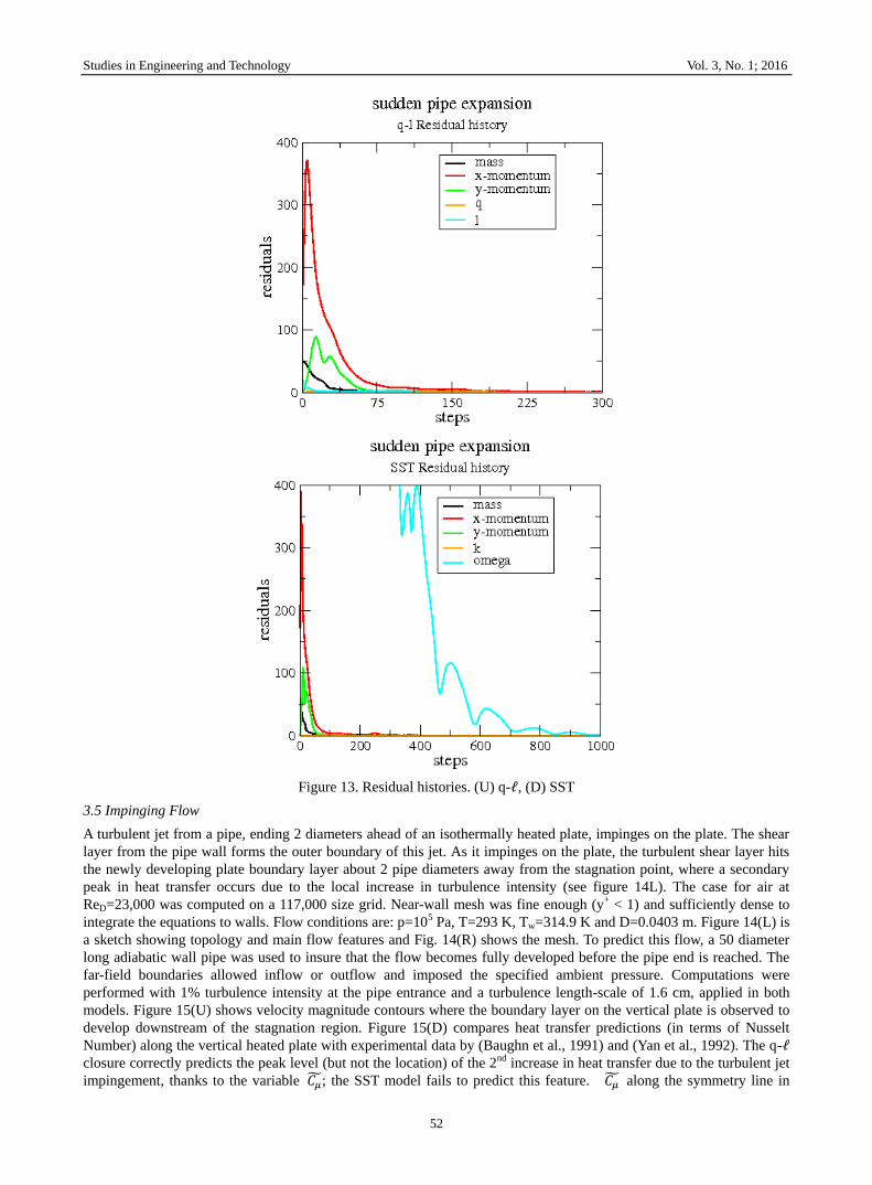
overpredicts by 60%. Lastly, residual histories are seen in Fig. 13. Due to , the SST model required 1000 steps to

converge whereas q-ℓ converged in 200 steps.

Studies in Engineering and Technology Vol. 3, No. 1; 2016

51

Figure 11. (U) Sketch of geometry, (D) Flow details

Figure 12. (L) Negative velocity contours, (R) Heat transfer profiles

Studies in Engineering and Technology Vol. 3, No. 1; 2016

52

Figure 13. Residual histories. (U) q-ℓ, (D) SST

3.5 Impinging Flow

A turbulent jet from a pipe, ending 2 diameters ahead of an isothermally heated plate, impinges on the plate. The shear

layer from the pipe wall forms the outer boundary of this jet. As it impinges on the plate, the turbulent shear layer hits

the newly developing plate boundary layer about 2 pipe diameters away from the stagnation point, where a secondary

peak in heat transfer occurs due to the local increase in turbulence intensity (see figure 14L). The case for air at

ReD=23,000 was computed on a 117,000 size grid. Near-wall mesh was fine enough (y+ < 1) and sufficiently dense to

integrate the equations to walls. Flow conditions are: p=105 Pa, T=293 K, Tw=314.9 K and D=0.0403 m. Figure 14(L) is

a sketch showing topology and main flow features and Fig. 14(R) shows the mesh. To predict this flow, a 50 diameter

long adiabatic wall pipe was used to insure that the flow becomes fully developed before the pipe end is reached. The

far-field boundaries allowed inflow or outflow and imposed the specified ambient pressure. Computations were

performed with 1% turbulence intensity at the pipe entrance and a turbulence length-scale of 1.6 cm, applied in both

models. Figure 15(U) shows velocity magnitude contours where the boundary layer on the vertical plate is observed to

develop downstream of the stagnation region. Figure 15(D) compares heat transfer predictions (in terms of Nusselt

Number) along the vertical heated plate with experimental data by (Baughn et al., 1991) and (Yan et al., 1992). The q-ℓ

closure correctly predicts the peak level (but not the location) of the 2nd increase in heat transfer due to the turbulent jet

impingement, thanks to the variable 𝐶�̃�; the SST model fails to predict this feature. 𝐶�̃� along the symmetry line in

Studies in Engineering and Technology Vol. 3, No. 1; 2016

53

shown in Fig. 16(L). While the flow is not fully developed along the pipe, 𝐶�̃� 𝐶𝜇 < 1⁄ but once fully developed,

𝐶�̃� 𝐶𝜇 ≅ 1⁄ . As the stagnation point is approached (0), 𝐶�̃� 𝐶𝜇 ≈ 𝐵𝑆̅ (𝐶𝜇𝑆̅𝐴)⁄ = 𝐵 (𝐶𝜇𝑆̅𝐴−1)⁄ ≪ 1⁄ but immediately

reaches 1 at the impingement point where 𝑆 = 𝜕𝑈 𝜕𝑥 → 0⁄ .

Both models converged more than 5 orders of magnitude, as seen in Fig. 16(R) for q-ℓ.

Figure 14. (L) Sketch of geometry and flow features, (R) grid

Figure 15. (U) Velocity magnitude contours, (D) Heat transfer profiles along vertical wall

Studies in Engineering and Technology Vol. 3, No. 1; 2016

54

Figure 16. (L) Variable Cμ, (R) Residuals history

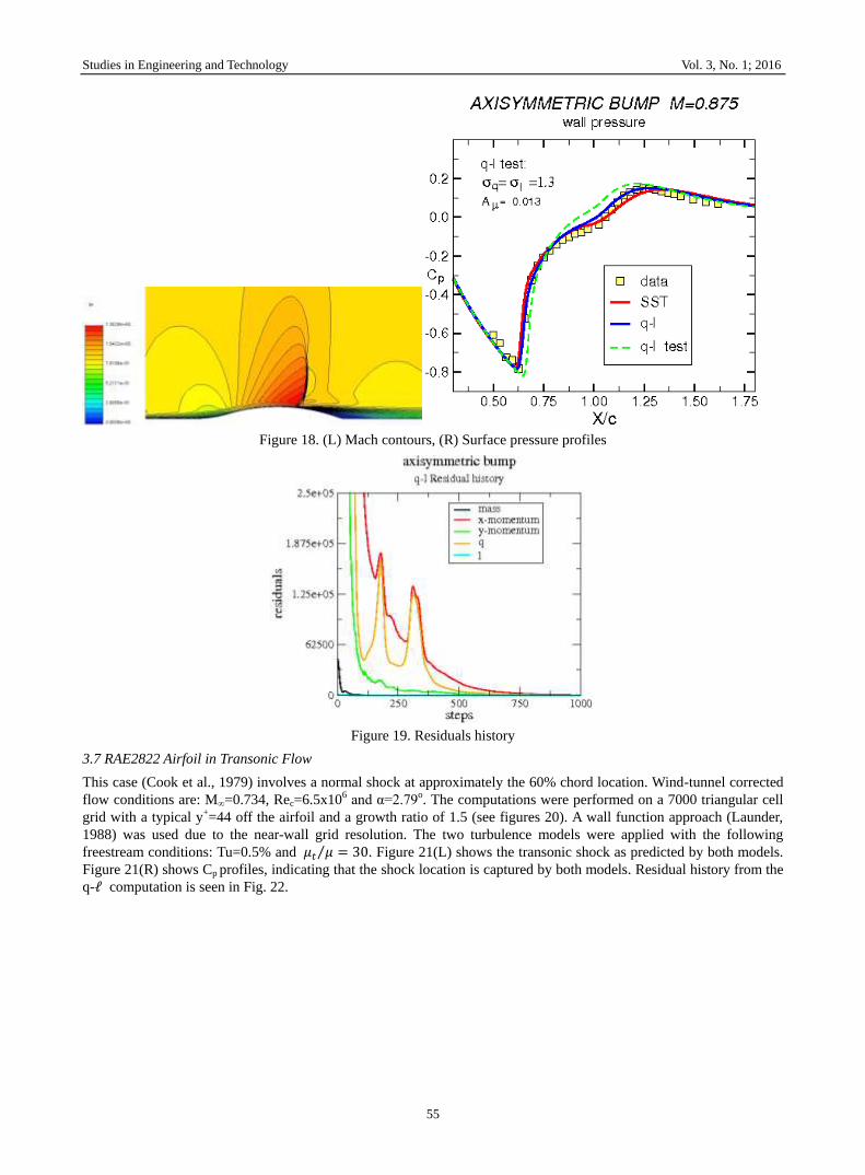
3.6 Transonic Flow over an Axisymmetric Bump (Bachalo & Johnson, 1979)

Figure 17 shows geometry and main flow features of this case. A normal shock, interacting with the boundary layer,

causes flow detachment over the bump, at x/c ≈ 0.7, with subsequent reattachment on the downstream cylindrical

portion. Inflow conditions are: M∞=0.875, Re∞,=1.36x107 at x=1m, p∞=57,935 Pa, T∞=255.6 K, Tu=1% and μt/μ=20.

The turbulence models were used on a 12,000 cell grid with y+ ≤ 1 to permit direct solution to the wall. Figure 18(L)

shows Mach contours where the normal shock is observed. Fig. 18(R) compares wall pressure prediction with data,

showing accurate capture of shock location by both turbulence closures, yet a marginally better shock capture is

predicted by the q-ℓ model. This figure includes a result with the ‘test’ q-ℓ version (𝜎𝑞 = 𝜎ℓ = 1.3, 𝐴𝜇 = 0.013)

mentioned earlier. Evidently the result is inferior to the proposed version (𝜎𝑞 = 𝜎ℓ = 1.0, 𝐴𝜇 = 0.023).

Figure 19 shows residual history. 18 orders of magnitude reduction in residuals were achieved by both models.

Figure 17. Geometry and main flow features

Studies in Engineering and Technology Vol. 3, No. 1; 2016

55

Figure 18. (L) Mach contours, (R) Surface pressure profiles

Figure 19. Residuals history

3.7 RAE2822 Airfoil in Transonic Flow

This case (Cook et al., 1979) involves a normal shock at approximately the 60% chord location. Wind-tunnel corrected

flow conditions are: M∞=0.734, Rec=6.5x106 and α=2.79o. The computations were performed on a 7000 triangular cell

grid with a typical y+=44 off the airfoil and a growth ratio of 1.5 (see figures 20). A wall function approach (Launder,

1988) was used due to the near-wall grid resolution. The two turbulence models were applied with the following

freestream conditions: Tu=0.5% and 𝜇𝑡 𝜇 = 30⁄ . Figure 21(L) shows the transonic shock as predicted by both models.

Figure 21(R) shows Cp profiles, indicating that the shock location is captured by both models. Residual history from the

q-ℓ computation is seen in Fig. 22.

Studies in Engineering and Technology Vol. 3, No. 1; 2016

56

Figure 20. (L) Triangular mesh, (R) Near-wall grid detail

Figure 21. (L) Mach contours (shock at x/c ~ 0.6), (R) Surface pressure profiles

Figure 22. Residuals history

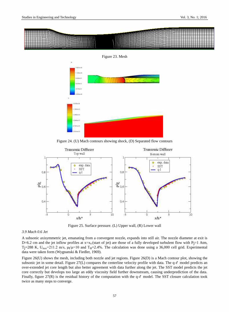
3.8 Transonic Diffuser

(Mohler, 2005) describes a 2D transonic diffuser test case in which a subsonic inflow accelerates to supersonic levels

within a nozzle-like geometry, then shocks down to subsonic flow in the diverging (diffuser) portion. The shock causes

flow separation on the curved (top) wall with consequent reattachment upstream of the exit. Figure 23 shows geometry

and mesh. Fig. 24(U) shows Mach contours where the shock and separation bubble downstream of it are seen. Fig. 24(D)

shows negative streamwise velocity contours, depicting the separation bubble.

Flow conditions: po,in=134.4 kPa, To,in=277.8 K, pout=97.2 kPa, Tu=0.5%, μt/μ=50.

This case was run on a 21,000 cell mesh with y+ ≤ 0.2 on both walls to permit direct solution to the wall.

Figures 25 compare pressure predictions along both walls with experimental data, showing accurate capture of the

measured data, including shock locations, by both models. Here h* is the throat height.

Studies in Engineering and Technology Vol. 3, No. 1; 2016

57

Figure 23. Mesh

Figure 24. (U) Mach contours showing shock, (D) Separated flow contours

Figure 25. Surface pressure. (L) Upper wall, (R) Lower wall

3.9 Mach 0.6 Jet

A subsonic axisymmetric jet, emanating from a convergent nozzle, expands into still air. The nozzle diameter at exit is

D=6.2 cm and the jet inflow profiles at x=x0 (start of jet) are those of a fully developed turbulent flow with Pj=1 Atm,

Tj=288 K, Umax=211.2 m/s, μt/μ=10 and Tu=2.4%. The calculation was done using a 36,000 cell grid. Experimental

data were taken form (Wygnanski & Fiedler, 1969).

Figure 26(U) shows the mesh, including both nozzle and jet regions. Figure 26(D) is a Mach contour plot, showing the

subsonic jet in some detail. Figure 27(L) compares the centerline velocity profile with data. The q-ℓ model predicts an

over-extended jet core length but also better agreement with data further along the jet. The SST model predicts the jet

core correctly but develops too large an eddy viscosity field further downstream, causing underprediction of the data.

Finally, figure 27(R) is the residual history of the computation with the q-ℓ model. The SST closure calculation took

twice as many steps to converge.

Studies in Engineering and Technology Vol. 3, No. 1; 2016

58

Figure 26. (U) Geometry and mesh, (D) Mach contours

Figure 27. (L) Centerline velocity profiles, (R) q-ℓ Residuals history

3.10 Reattaching Supersonic Shear Layer

(Samimy et al., 1986) report experimental results from a supersonic turbulent reattaching shear layer onto a slanted

ramp (see Figures 28 for topology). Freestream conditions are: M∞

=2.46, Re∞

=5x107/m, po

=528.1 kPa and To

=297 K.

An inflow boundary layer with δ=3.12 mm was imposed on both walls. A 52,500 cell grid was used for the calculation

with y+≤ 0.3 and a small growth rate of 1.15 to enable direct solution to walls. The turbulence models were invoked

subject to Tu=1% and ℓT

=3 mm at inflow.

Figure 28(R) shows Mach contours where the reattaching shear layer and recompression shock are clearly seen. Figure

29(L) shows negative streamwise velocity contours, indicating that shear layer reattachment is predicted by the q-ℓ

model at x≈140 mm, about 7.5% further downstream than indicated by measurements. The corresponding numbers for

SST are x=138 mm, 6% downstream of the data. Figure 29 (R) compares predicted lower wall pressure distribution

with the data, showing that the two predictions are practically identical and follow the measurements. Fig. 30 shows

residuals history with the q-ℓ model computation.

Studies in Engineering and Technology Vol. 3, No. 1; 2016

59

Figure 28. (L) mesh, (R) Mach contours showing shear layer

Figure 29. (L) Separated flow velocity contours, (R) Lower wall pressure profiles

Figure 30. Residual history with q-ℓ

3.11 Flow over Hump

Turbulent flow separation over a hump was studied numerically and experimentally (Chuan et al., 2007), this being a

canonical turbulent separated flowfield case. The hump is the upper surface of a modified Glauert airfoil which consists

of a relatively long fore-body and a short separation ramp at the trailing edge (Figure 31(U). This shape was selected

because the separation location is insensitive to Reynolds number and detailed experimental data are well-documented

in the literature (Chuan et al., 2007). The hump has a physical chord length of c = 420 mm and a maximum height of

53.7 mm. The inlet is located at x/c = −6.39 where the freestream Mach number is set to be 0.1 (U∞ = 34.6 m/s). The

outlet is located at x/c = 4.0 where the pressure is set to p/p∞ = 0.99962. The flat top-wall is located at y/c = 0.9.

Non-slip conditions were applied at the top-wall, floor and hump surface.

The computation was done on a 208,000 cell grid with y+≤ 0.5 over the hump wall and a growth rate of 1.01, permitting

direct solve-to-wall. A portion of the grid is shown in Fig. 31(D).

The turbulence closures were used subject to the following inflow conditions: Tu=0.5% and μt/μ=20.

Studies in Engineering and Technology Vol. 3, No. 1; 2016

60

Fig. 32(L) shows the separated flow bubble and Fig. 32(R) is a plot of residual history by the q-ℓ model.

Figures 33 show surface pressure and skin friction predictions along the hump. Both models over-predict the separation

bubble extent, more so by the q-ℓ closure. The pressure prediction, Fig. 33(L), is done well by both models down to

x=0.4 m, deteriorating further downstream due to the overprediction of the separation bubble size.

Figure 31. (U) Hump topology, (D) Mesh detail

Figure32. (L) Separated flow contours, (R) Residuals plot

Figure 33. (L) Pressure profiles, (R) Skin friction profiles

3.12 ARA M100 Wing/Body

This wing/body test case (Peigin & Epstein, 2004) is at α= 2.870, M∞=0.803 and aerodynamic chord Reynolds number

Studies in Engineering and Technology Vol. 3, No. 1; 2016

61

Rec = 13.1x106. The mesh (cfl3d.larc.nasa.gov) has 860,000 cells with an off-wall y+ distribution as follows:

y+wing=0.8, 0.1≤ y+

fuselage≤ 30. Consequently, a wall function (Launder, 1988) was used over the fuselage and direct

solve-to-wall was employed on the wing where the grid growth rate is 1.09. Freestream turbulence levels were Tu=0.5%

and µt/µ=25. Figure 34 shows pressure contours on the fuselage and upper wing surface. The normal shock footprint on

the wing’s suction side is observed. Figure 35(U) is that of a wing slice at =0.455, showing the normal shock and its

interaction with the turbulent boundary layer. Fig. 35(D) provides a clear picture of the shock foot along the wing span

by showing surface pressure contours. Cp profiles at two wing sections are seen in figures 36. Comparisons with

experimental data show that the shock location, predicted by the q-ℓ model at =0.455, is closer to the data than that by

the SST closure but the opposite prevails at =0.935 (close to the wing tip). Finally, Fig. 37 shows the residuals

history from the q-ℓ calculation.

Figure 34. Topology and pressure contours showing shock along wing

Figure 35. (U) Wing section Mach contours showing shock and flow separation, (D) wing suction side pressure

contours showing shock foot along wing span

Studies in Engineering and Technology Vol. 3, No. 1; 2016

62

Figure 36. Pressure profiles. (L) at =0.455, (R) at =0.935

Figure 37. Residual history

4. Summary and Conclusions

A two-equation √𝑘 − ℓ turbulence model was introduced and tested. The model does not involve topological

parameters like wall distance, instead it resorts to a number of local wall proximity indicators, an important benefit for

engineering purposes. While the model is linear, it incorporates a variable 𝐶�̃� coefficient which sensitizes it to flows

involving non-simple shear such as impingement or stagnation zones. Both model variables are subject to simple

Diriclet wall boundary conditions and q is linear across the viscous sublayer, rendering the closure numerically robust

and forgiving less than ideal near-wall grid concentration (as long as enough mesh exists to capture the turbulent

near-wall behavior).

The q- ℓ model was tested on a wide variety of flows, including low and high speed, internal and external, 2D and 3D.

Compared to predictions by the SST closure (which requires wall distance), q- ℓ performs better in cases involving

impinging or semi-stagnating flows (as in the pipe sudden expansion flow at reattachment) but may overpredict

separation bubble extents in some low-speed flows. In both internal and external transonic flows the two models’

predictions are close.

Fluids engineers whose work involves complex 3D topologies, particularly for non-stationary grids which require

re-computing wall distance arrays at each time-step, may appreciate the fact that no distance arrays are needed for the

q- ℓ model.

References

Bachalo, W. D., &. Johnson, D. A. (1979). An Investigation of Transonic Turbulent Boundary Layer Separation

Generated on an Axisymmetric Flow Model. AIAA Paper 79-1479. http://dx.doi.org/10.2514/6.1979-1479

Batten, P., Leschziner, M. A., & Goldberg, U. C. (1997). Average-State Jacobians and Implicit Methods for

Compressible Viscous and Turbulent Flows. J. of Computational Physics., 137, 38-78.

http://dx.doi.org/10.1006/jcph.1997.5793

Studies in Engineering and Technology Vol. 3, No. 1; 2016

63

Baughn, J. W., Hechanova, A., & Yan, X. (1991). An Experimental Study of Entrainment Effects on the Heat Transfer

from a Flat Plate Surface to a Heated Circular Impinging Jet. ASME J. Heat Transfer 113, 1023-1025.

http://dx.doi.org/10.1115/1.2911197

Baughn, J. W., Hoffman, M. A., Launder, B. E., Lee, D., & Yap, C. (1989). Heat Transfer, Temperature, and Velocity

Measurements Downstream of an Abrupt Expansion in a Circular Tube at a Uniform Wall Temperature. ASME

Journal of Heat Transfer, 111, 870-876. http://dx.doi.org/10.1115/1.3250799

Buice, C. U., & Eaton, J. K. (2000). Experimental Investigation of Flow Through an Asymmetric Plane Diffuser.

Journal of Fluids Engineering, 122, 433-435. http://dx.doi.org/10.1115/1.483278

Chakravarthy, S. (1999). A Unified-Grid Finite Volume Formulation for Computational Fluid Dynamics. Int. J. Numer.

Meth. Fluids, 31, 309-323.

http://dx.doi.org/10.1002/(SICI)1097-0363(19990915)31:1<309::AID-FLD971>3.0.CO;2-M

Chuan, H., Corke, T. C., & Patel, M. P. (2007). Numerical and Experimental Analysis of Plasma Flow Control Over a

Hump Model, AIAA Paper 2007-0935, 45th Aerospace Sciences Meeting, Reno, Nevada.

Cook, P. H., McDonald, M. A., & Firmin, M. C. P. (1979). Aerofoil RAE 2822 - Pressure Distributions, and Boundary

Layer and Wake Measurements, Experimental Data Base for Computer Program Assessment. AGARD Report AR

138.

Driver, D. M. (1991). Reynolds Shear Stress Measurements in a Separated Boundary Layer Flow. AIAA Paper 91-1787,

AIAA 22nd Fluid Dynamics, Plasma Dynamics, and Lasers Conference, Honolulu, HI.

http://dx.doi.org/10.2514/6.1991-1787

Goldberg, U., Batten, P., & Palaniswamy, S. (2004). The q-ℓ Turbulence Closure for Wall-Bounded and Free Shear

Flows. AIAA Paper 2004-269, 42nd AIAA Aerospace Sciences Meeting and Exhibit, Reno, Nevada.

http://dx.doi.org/10.2514/6.2004-269

Goldberg, U. (2006). A k-ℓ Turbulence Closure Sesitized to Non-Simple Shear Flows. Int. J. of Computational Fluid

Dynamics, 20(9), 651-656. http://dx.doi.org/10.1080/10618560701259257

Goldberg, U., & Apsley, D. (1997). A Wall-Distance-Free Low Re k-ε Turbulence Model. Computer methods in

applied mechanics and engineering, 145, 227-238. http://dx.doi.org/10.1016/S0045-7825(96)01202-9

Launder, B. E. (1988). On the Computation of Convective Heat Transfer in Complex Turbulent Flows. Transactions of

the ASME, 110, 1112-1128. http://dx.doi.org/10.1115/1.3250614

Menter, F. R., Kuntz, M., & Langtry, R. (2003). Ten Years of Industrial Experience with the SST Turbulence Model.

Turbulence, Heat and Mass Transfer 4, Hanjalic K, Nagano Y, Tummers M. (Eds.). Begell House, Inc., 625–632.

Mohler, S. R. (2005). Wind-US Unstructured Flow Solutions for a Transonic Diffuser. NASA CR-2005- 213417.

http://dx.doi.org/10.2514/6.2005-1004

Peroomian, O., Chakravarthy, S., & Goldberg, U. (1997). A ‘Grid-Transparent’ Methodology for CFD. AIAA Paper

97-0724. http://dx.doi.org/10.2514/6.1997-724

Peroomian, O., Chakravarthy, S., Palaniswamy, S., & Goldberg, U. (1998). Convergence Acceleration for Unified-Grid

Formulation using Preconditioned Implicit Relaxation. AIAA, 98-0116. http://dx.doi.org/10.2514/6.1998-116

Peigin, S., & Epstein, B. (2004). Embedded Parallelization Approach for Optimization in Aerodynamic Design. Journal

of Supercomputing, 29(3), 243-263. http://dx.doi.org/10.1023/B:SUPE.0000032780.68664.1b

Rumsey, C. L. Turbulence Modeling Resource. http://turbmodels.larc.nasa.gov/

Samimy, M.,. Petrie, H. L., & Addy, A. L. (1986). A Study of Compressible Turbulent Reattaching Free Shear Layers.

AIAA Journal, 24(2), 261-267. http://dx.doi.org/10.2514/3.9254

White, F. M. (1974). Viscous Fluid Flow. McGraw-Hill, p. 644.

Wygnanski, I., & Fiedler, H. (1969). Some Measurements in the Self-Preserving Jet. J. Fluid Mech., 38, 577–612.

http://dx.doi.org/10.1017/S0022112069000358

Yan, X., Baughn, J. W., & Mesbah, M. (1992). The effect of Reynolds number on the heat transfer distribution from a

flat plate to an impinging jet. ASME Heat Transfer Division, 226, 1-7.

This work is licensed under a Creative Commons Attribution 3.0 License.