AAS 12-624

A K-VECTOR APPROACH TO SAMPLING, INTERPOLATION, ANDAPPROXIMATION

Daniele Mortari∗ and Jonathan Rogers†

The k-vector search technique is a method designed to perform extremely fastrange searching of large databases at computational cost independent of the sizeof the database. k-vector search algorithms have historically found applicationin satellite star-tracker navigation systems which index very large star cataloguesrepeatedly in the process of attitude estimation. Recently, the k-vector search al-gorithm has been applied to numerous other problem areas including non-uniformrandom variate sampling, interpolation of 1-D or 2-D tables, nonlinear functioninversion, and solution of systems of nonlinear equations. This paper presentsalgorithms in which the k-vector search technique is used to solve each of theseproblems in a computationally-efficient manner. In instances where these tasksmust be performed repeatedly on a static (or nearly-static) data set, the proposedk-vector-based algorithms offer an extremely fast solution technique that outper-forms standard methods.

Truth is much too complicated to allow anything but approximations (John von Newman, 1947).

INTRODUCTION

The k-vector search method is a range searching technique devised [1] within the general problemof spacecraft attitude determination for the lost-in-space case, when no estimate of the spacecraftattitude is available. In particular, the technique was developed to accelerate the Star-ID problemof wide field-of-view (FOV) star trackers. Using the k-vector technique, the Star-ID SearchlessAlgorithm was first proposed in [2]. The k-vector search method requires the construction of avector of integers of length n, the k-vector, whose entries contain information to solve the searchingproblem. Use of the k-vector vastly reduces the search effort required, which constitutes the heaviestcomputational burden of Star-ID algorithms. Since its initial development, the k-vector techniquehas been applied in various Star-ID approaches: the SP-Search [3], multiple FOV star trackers [4, 5],and the LISA algorithm [6] for the StarNav I test experiment onboard STS-107.

One of the most important considerations when using the k-vector is that it is primarily suitableonly for static databases (e.g., inter-star angles are time-invariant). In other words, ideal perfor-mance is achieved if data is not inserted, deleted, or changed within the database. Recognizingthat the k-vector technique is a general mathematical tool to solve the range searching problem, theauthors extended the k-vector algorithm in [7] to explore its potential in new applications other than

∗Professor, 746C H.R. Bright Bldg, Aerospace Engineering, Texas A&M University, College Station, TX 77843-3141, Tel.: (979) 845-0734, Fax: (979) 845-6051, AIAA Associate Fellow. IEEE senior member. E-mail: MOR-TARI@TAMU.EDU†Assistant Professor, 746B H.R. Bright Bldg, Aerospace Engineering, Texas A&M University, College Station, TX 77843-3141, Tel.: (979) 862-3413, Fax: (979) 845-6051. E-mail: JROGERS@AERO.TAMU.EDU

1

the Star-ID problem. This new searching technique became the heart of “Pyramid” [8], the currentstate-of-the-art in Star-ID algorithms, which has been flying onboard the MIT HETE and HETE-2missions as well as several other satellites. However, application of the k-vector technique to thispoint has largely been limited to the original Star-ID application.

This study explores techniques to apply k-vector search methods to a broader class of problems,of which Star-ID is one specific single application. Specific areas of interest include efficient non-linear function inversion, minimal search table interpolation, and random variate sampling from anarbitrary density function. In each application, emphasis is placed on minimizing computationalburden with respect to current state-of-the-art methods. The paper is organized as follows. First,background on the general k-vector search algorithm is presented. Then, a k-vector-based methodto invert nonlinear functions at discrete values is outlined, and specific 1-D and 2-D examples areoffered. The method is also highly effective in computing intersections of nonlinear functions ofarbitrary dimension. Interpolation techniques using the k-vector are then discussed in the contextof static aerodynamic databases, which are typically indexed repeatedly during atmospheric vehiclesimulation. Finally, a k-vector approache to random variate sampling is presented with potentialapplications in the area of sensor simulation and particle filter resampling. Overall, the methodsdeveloped here promise to substantially reduce runtime requirements for many basic mathematicalalgorithms of interest to the science and engineering community.

Background on the k-vector

The range searching problem consists of identifying, within a large n-valued database y (n� 1),the set of all data elements y(I), where I is a vector of indices, such that y(I) ∈ [ya, yb], where ya <yb. This problem is usually solved using the Binary Search Technique (BST), whose complexity isO(2 log2 n) in sorted databases (where 2 log2 n represents the number of comparisons in the worstcase). Many variants of BSTs have been introduced [9] for use in particular applications in order tominimize the searching time.

The k-vector technique is summarized as follows. Let y be an data vector of n elements (n� 1)and s the same vector but sorted in ascending mode, i.e. s(i) ≤ s(i+ 1). Let s(i) = y(I(i)), whereI is the integer vector of the sorting with length n. In particular, we have ymin = min

iy(i) = s(1)

and ymax = maxi

y(i) = s(n).

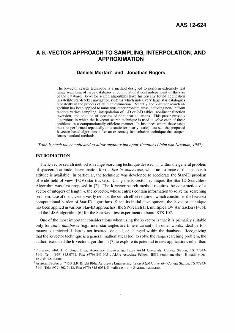
As shown in Fig. 1,∗ the line connecting the two extreme points, [1, ymin] and [n, ymax], has onaverage, E0 = n/(n−1) elements for each d = (ymax−ymin)/(n−1) step. However, we considera slightly steeper line connecting the points [1, ymin − δε] and [n, ymax + δε], where δε = (n− 1)εand ε is the relative machine precision (ε ≈ 2.22×10−16 for double precision arithmetic)†. Thisslightly steeper line assures k(1) = 0 and k(n) = n, thus simplifying the code by avoiding manyindex checks. The equation of this line can be written as

z(x) = mx+ q where{m = (ymax − ymin + 2δε)/(n− 1)q = ymin −m− δε

(1)

Setting k(1) = 0 and k(n) = n, the i-th element of the k-vector is

k(i) = j where j is the greatest index such that s(j) ≤ y(I(i)) is satisfied. (2)∗Figures 1 and 2 has been taken from Ref. [7].†The expression provided for δε comes from the proportionality,

ymax − ymin

δε=

(ymax − ymin)/(n− 1)

ε.

2

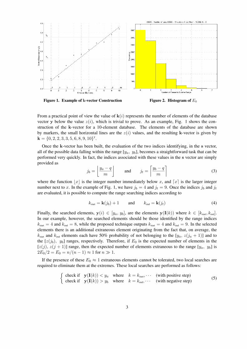
Figure 1. Example of k-vector Construction Figure 2. Histogram of E0

From a practical point of view the value of k(i) represents the number of elements of the databasevector y below the value z(i), which is trivial to prove. As an example, Fig. 1 shows the con-struction of the k-vector for a 10-element database. The elements of the database are shownby markers, the small horizontal lines are the z(i) values, and the resulting k-vector is given byk = {0, 2, 2, 3, 3, 5, 6, 8, 9, 10}T.

Once the k-vector has been built, the evaluation of the two indices identifying, in the s vector,all of the possible data falling within the range [ya, yb], becomes a straightforward task that can beperformed very quickly. In fact, the indices associated with these values in the s vector are simplyprovided as

jb =

⌊ya − qm

⌋and jt =

⌈yb − qm

⌉(3)

where the function bxc is the integer number immediately below x, and dxe is the larger integernumber next to x. In the example of Fig. 1, we have jb = 4 and jt = 9. Once the indices jb and jtare evaluated, it is possible to compute the range searching indices according to

kstart = k(jb) + 1 and kend = k(jt) (4)

Finally, the searched elements, y(i) ∈ [ya, yb], are the elements y(I(k)) where k ∈ [kstart, kend].In our example, however, the searched elements should be those identified by the range indiceskstart = 4 and kend = 8, while the proposed technique outputs kstart = 4 and kend = 9. In the selectedelements there is an additional extraneous element originating from the fact that, on average, thekstart and kend elements each have 50% probability of not belonging to the [ya, z(ja + 1)] and tothe [z(jb), yb] ranges, respectively. Therefore, if E0 is the expected number of elements in the[z(j), z(j + 1)] range, then the expected number of elements extraneous to the range [ya, yb] is2E0/2 = E0 = n/(n− 1) ≈ 1 for n� 1.

If the presence of these E0 ≈ 1 extraneous elements cannot be tolerated, two local searches arerequired to eliminate them at the extremes. These local searches are performed as follows:{

check if y(I(k)) < ya where k = kstart, · · · (with positive step)check if y(I(k)) > yb where k = kend, · · · (with negative step)

(5)

3

For large databases (n�1), since limn→∞

E0 = 1, the number of searched data can be approximatedby nd = kend − kstart, since only E0 ≈ 1 extraneous elements are expected. Thus, on average,the method provides the solution with only three comparisons‡ and therefore exhibites complexityO(3), which is independent from the database size. For n � 1, this algorithmic complexity issignificantly less than O(2 log2 n) as required by BST. This value of complexity holds if the k-vector behavior is linear or quasi-linear with respect to the indices. Strong nonlinear behavior hasbeen analyzed in Ref. [7]. For instance, a worst-case scenario occurs when (n− 2) data fall withina single range step [z(i), z(i+ 1)]. In this case, however, the k-vector can be built within this rangeusing (n−2) data instead of n. Another worst case scenario occurs when the k-vector distribution ispiecewise linear, in which case a different k-vector should be built for each different linear segment.

To validate the statistics of the number of extraneus elements, an 65535-element§ vector y wasrandomly created and the associated k-vector generated. Figure 2 shows the histogram of E0 (theextraneous elements), obtained in 10,000 trials, is given. The numerical mean value obtained is1.0032, which agrees with the theoretical expected value E0 = 65535/(65535− 1) = 1.000015¶.

K-VECTOR TO INVERT NONLINEAR N -DIMENSIONAL FUNCTIONS

The k-vector exhibits computational advantages when applied to static databases, and can thusbe used effectively to invert nonlinear n-dimensional functions. The k-vector approach to performfunction inversion is given as follows. Let y = f(x) be a nonlinear function of n independentvariables (where n is the dimensionality of x). Examples of n = 1 mathematical problems involvingthe inversion of nonlinear functions are:

1. Find the values of x at which the function y = f(x) assumes an assigned known value y. Anelementary example is to find the roots of the nonlinear function f(x) = 0;

2. Find the values of a parameter p such that∫ xmax

xmin

f(x, p) dx = y, where xmin and xmax are

assigned. For instance, this problem occurs when trying to invert the complete elliptic integralof the first kind (find k)

K(k) =

∫ π/2

0

1√1− k2 sin2 θ

dθ =

∫ 1

0

1√(1− t2)(1− k2 t2

dt

or the complete elliptic integral of the second kind

E(k) =

∫ π/2

0

√1− k2 sin2 θ dθ =

∫ 1

0

√1− k2 t2√

1− t2dt

3. Find the value(s) of the integration bounds of an integral,∫ x

xmin

f(ξ) dξ = y or∫ xmax

xf(ξ) dξ =

y. Some examples commonly found in scientific problems are:

(a) the logarithmic integral function, li(x) =

∫ x

0

1

ln tdt,

‡One for each check given in Eq. (5) plus the comparison needed to identify the E0 ≈ 1 extraneous element.§The number of elements is 65535 = 216 − 1 so that each element index can be stored in 2-bytes.¶The small difference between experimental and theoretical values comes from the fact that, when kend = kstart + 1

occurs, then the number of expected extraneous elements becomes E0/2.

4

(b) the exponential integral‖, Ei(x) =

∫ x

−∞

et

tdt,

(c) the sin and cosine integrals Si(x) =

∫ x

0

sin t

tdt and Ci(x) = γ+lnx+

∫ x

0

cos t− 1

tdt,

where γ = limn→∞

[n∑k=1

1

k− ln(n)

]= lim

b→∞

∫ b

1

(1

bxc− 1

x

)dx ≈ 0.577215665 is the

Euler-Mascheroni constant,

(d) the hyperbolic sine and cosine integrals, Shi(x) =

∫ x

0

sinh t

tdt and Chi(x) = γ +

lnx+

∫ x

0

cosh t− 1

tdt,

(e) the error function, erf(x) =2√π

∫ x

0e−t

2dt,

(f) the Fresnel integrals, S(x) =

∫ x

0sin(t2) dt and C(x) =

∫ x

0cos(t2) dt,

(g) the Dawson integral, D+(x) = e−x2

∫ x

0et

2dt and D−(x) = ex

2

∫ x

0e−t

2dt,

(h) the Digamma function, ψ(x) =

∫ ∞0

(e−t

t− e−xt

1− e−t

)dt,

(i) the Polygamma function, ψ(m)(x) = (−1)m+1

∫ ∞0

tm e−xt

1− e−tdt,

(j) and Bessel’s integrals, Jn(x) =1

π

∫ π

0cos(nt− x sin t) dt,

The Methodology

The k-vector methodology for function inversion may be explained through an example. Con-

sider the problem of inverting the Fresnel integral, y =

∫ x

0sin(t2) dt between the x ∈ [0, 5] range.

The goal is to construct a numerical procedure that solves for all roots, xk ∈ [0, 5], for any givenvalue of the integral. Before proceeding with the description of the algorithm it is important todefine the limits in applying the proposed methodology:

1. The proposed method is not suitable to invert a nonlinear function just for a single time,for which other methods may be more efficient. Since the proposed method requires somepreprocessing efforts (see Fig. 4 for the algorithm), its efficiency is exposed when the func-tion inversion problem must be performed extensively in some assigned range for the samenonlinear function. Once the preprocessing has been completed, the inverting function canbe created and used anytime, either extensively or just for a single shot. For instance, theproposed methodology is suitable for creating fast built-in inversion functions for MATLAB.

‖To get an idea of the many applications of Ei(x), Ref. [10] mentioned: a) Time-dependent heat transfer, b) Nonequi-librium groundwater flow in the Theis solution (called a well function), c) Radiative transfer in stellar atmospheres, d)Radial Diffusivity Equation for transient or unsteady state flow with line sources and sinks, and e) Solutions to the neutrontransport equation in simplified 1-D geometries.

5

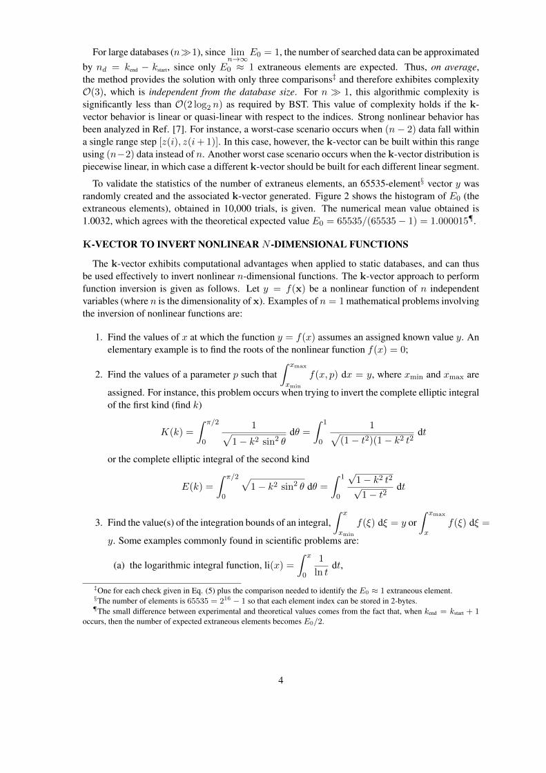
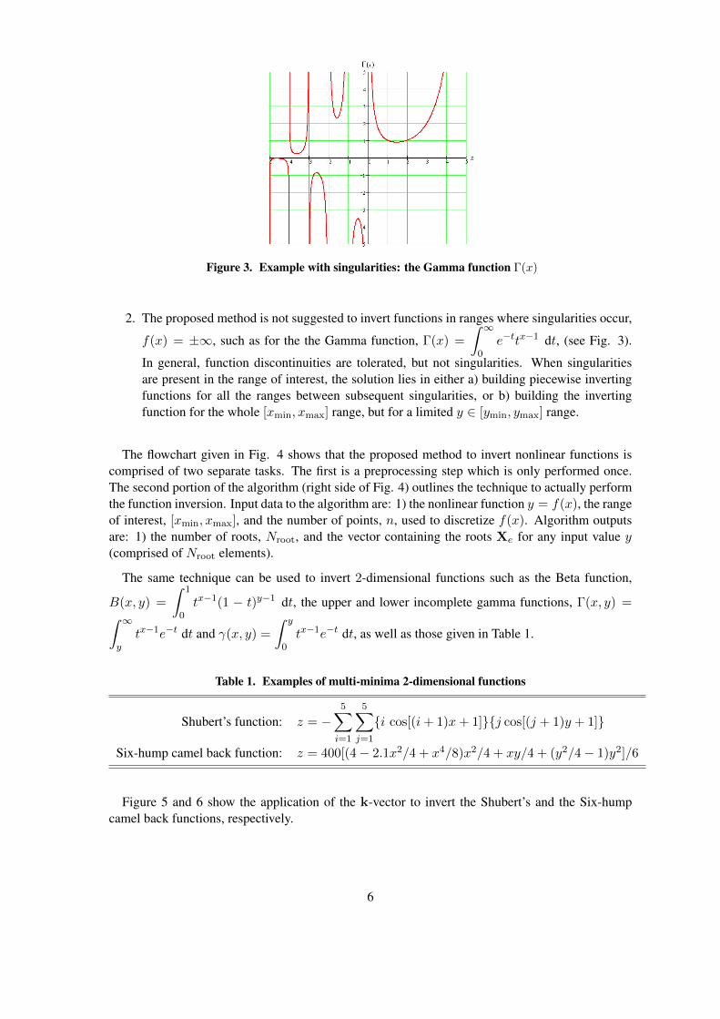
Figure 3. Example with singularities: the Gamma function Γ(x)

2. The proposed method is not suggested to invert functions in ranges where singularities occur,

f(x) = ±∞, such as for the the Gamma function, Γ(x) =

∫ ∞0

e−ttx−1 dt, (see Fig. 3).

In general, function discontinuities are tolerated, but not singularities. When singularitiesare present in the range of interest, the solution lies in either a) building piecewise invertingfunctions for all the ranges between subsequent singularities, or b) building the invertingfunction for the whole [xmin, xmax] range, but for a limited y ∈ [ymin, ymax] range.

The flowchart given in Fig. 4 shows that the proposed method to invert nonlinear functions iscomprised of two separate tasks. The first is a preprocessing step which is only performed once.The second portion of the algorithm (right side of Fig. 4) outlines the technique to actually performthe function inversion. Input data to the algorithm are: 1) the nonlinear function y = f(x), the rangeof interest, [xmin, xmax], and the number of points, n, used to discretize f(x). Algorithm outputsare: 1) the number of roots, Nroot, and the vector containing the roots Xe for any input value y(comprised of Nroot elements).

The same technique can be used to invert 2-dimensional functions such as the Beta function,

B(x, y) =

∫ 1

0tx−1(1 − t)y−1 dt, the upper and lower incomplete gamma functions, Γ(x, y) =∫ ∞

ytx−1e−t dt and γ(x, y) =

∫ y

0tx−1e−t dt, as well as those given in Table 1.

Table 1. Examples of multi-minima 2-dimensional functions

Shubert’s function: z = −5∑i=1

5∑j=1

{i cos[(i+ 1)x+ 1]}{j cos[(j + 1)y + 1]}

Six-hump camel back function: z = 400[(4− 2.1x2/4 + x4/8)x2/4 + xy/4 + (y2/4− 1)y2]/6

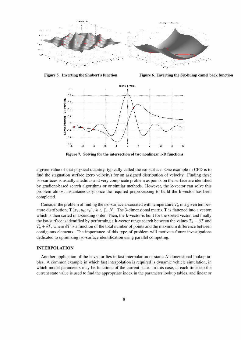
Figure 5 and 6 show the application of the k-vector to invert the Shubert’s and the Six-humpcamel back functions, respectively.

6

Figure 4. k-vector approach to invert the nonlinear function y = f(x) in x ∈[xmin, xmax] using n� 1 points.

Solving Systems of two Nonlinear n-Dimensional Functions

The proposed methodology can be applied in numerous interesting applications, including theproblem of finding solutions (values of x) of the following set of two equations

y = f(x) and y = g(x) + c (6)

where f(x) and g(x) can be any two given nonlinear functions and c a constant variable whosevalue may change. It is straightforward to show that Eq. (6) is equivalent to solving the followingequation

c = f(x)− g(x) = h(x). (7)

which can be done using the approach described in the previous section.

A 1-dimensional example of this problem is shown in Fig. 7 for the Dawson function f(x) =

D+(x) = e−x2

∫ x

0et

2dt and Sinc function g(x) =

sinx

x, while Fig. 8 shows a 2-dimensional

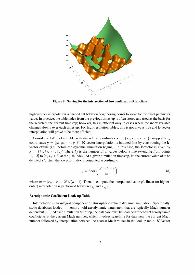
example using the Shubert’s and the Six-hump camel back functions given in Table 1.

Evaluation of iso-surfaces

Many scientific problems (i.e., computational fluid dynamics (CFD), combustion, atmosphericsciences, etc.) provide the 3-dimensional distribution of some physical quantity such as temperature,pressure, or velocity. It is of great interest to be able to quickly identify the surface associated with

7

Figure 5. Inverting the Shubert’s function Figure 6. Inverting the Six-hump camel back function

Figure 7. Solving for the intersection of two nonlinear 1-D functions

a given value of that physical quantity, typically called the iso-surface. One example in CFD is tofind the stagnation surface (zero velocity) for an assigned distribution of velocity. Finding theseiso-surfaces is usually a tedious and very complicate problem as points on the surface are identifiedby gradient-based search algorithms or or similar methods. However, the k-vector can solve thisproblem almost instantaneously, once the required preprocessing to build the k-vector has beencompleted.

Consider the problem of finding the iso-surface associated with temperature Ta in a given temper-ature distribution, T(xk, yk, zk), k ∈ [1, N ]. The 3-dimensional matrix T is flattened into a vector,which is then sorted in ascending order. Then, the k-vector is built for the sorted vector, and finallythe iso-surface is identified by performing a k-vector range search between the values Ta − δT andTa+ δT , where δT is a function of the total number of points and the maximum difference betweencontiguous elements. The importance of this type of problem will motivate future investigationsdedicated to optimizing iso-surface identification using parallel computing.

INTERPOLATION

Another application of the k-vector lies in fast interpolation of static N -dimensional lookup ta-bles. A common example in which fast interpolation is required is dynamic vehicle simulation, inwhich model parameters may be functions of the current state. In this case, at each timestep thecurrent state value is used to find the appropriate index in the parameter lookup tables, and linear or

8

Figure 8. Solving for the intersection of two nonlinear 2-D functions

higher-order interpolation is carried out between neighboring points to solve for the exact parametervalue. In practice, the table index from the previous timestep is often stored and used as the basis forthe search at the current timestep; however, this is efficient only in cases where the index variablechanges slowly over each timestep. For high-resolution tables, this is not always true and k-vectorinterpolation will prove to be more efficient.

Consider a 1-D lookup table with discrete x coordinates x = {x1, x2, · · · , xn}T mapped to ycoordinates y = {y1, y2, · · · , yn}T. K-vector interpolation is initiated first by constructing the k-vector offline (i.e., before the dynamic simulation begins). In this case, the k-vector is given byk = {k1, k2, · · · , kn}T where kj is the number of x values below a line extending from points[1,−δ] to [n, xn + δ] at the j-th index. At a given simulation timestep, let the current value of x bedenoted x∗. Then the k-vector index is computed according to

j = floor(x∗ − δ − q

m

)(8)

where m = (xn − x1 + 2δ)/(n− 1). Then, to compute the interpolated value y∗, linear (or higher-order) interpolation is performed between xkj and xkj+1.

Aerodynamic Coefficient Look-up Table

Interpolation is an integral component of atmospheric vehicle dynamic simulation. Specifically,static databases loaded in memory hold aerodynamic parameters that are typically Mach-numberdependent [19]. At each simulation timestep, the database must be searched for correct aerodynamiccoefficients at the current Mach number, which involves searching for data near the current Machnumber followed by interpolation between the nearest Mach values in the lookup table. K-Vector

9

Figure 9. Drag Coefficient vs Mach Number. Figure 10. k-vector for Lookup Table.

searching can locate the nearest Mach values and greatly increase computational efficiency sincethere is essentially no searching required.

Consider the zero-yaw drag force coefficient of the standard Army Navy Finner artillery projectile[20]. Figure 9 shows the Mach number dependence of this drag coefficient using 25 discrete points.Prior to a simulation, the k-vector can be constructed strictly from the Mach number data as shownin Figure 10. This k-vector represents the number of points whose corresponding Mach numberis below the point on a line at the given index (see above for k-vector construction algorithm).The static k-vector is then stored in memory, as are the slope m and the intercept q used to buildit. Suppose at the current timestep, the projectile is traveling at local Mach number 1.68. K-Vector interpolation of the drag coefficient table proceeds as follows. First, the k-vector index iscomputed using Equation 8, yielding a value of 9. The k-vector value at index 9 is 18, meaningthat the 18th Mach point (corresponding to Mach 1.5) is the point below Mach 1.68, as shownin Figure 9. Thus linear interpolation can be immediately performed between the 18th and 19thMach point with zero searching required. If model parameters are not reliably close to one anotherduring successive timesteps, the performance of a few algebraic calculations using the k-vectorinstead of searching methods could yield a significant reduction in runtime. This is particularlytrue of dynamic models that rely on large, static aerodynamic databases such as re-entry vehicles.Note that k-vector interpolation will only outperform standard search techniques (like BST) whendatabases are relatively large.

SAMPLING

K-vector techniques can also be used for intensive random number generation within the rangex ∈ [xmin, xmax], for an arbitrary continuous (or discrete) distribution, p(x). Let p(k) be a statisticalrealization of the density function p(x) composed of N � 1 points, where k ∈ [1, N ]. Also, lets(k) be the vector p(k) sorted in ascending order, i.e., s = p(I), where I is the sorting index vectorand s(k + 1) ≥ s(k) is the ascending sorting condition. Let k be the k-vector associated with thes vector. Using the sorted vector the range of the p vector is defined between pmin = s(1) andpmax = s(N).

Sampled data is then generated by performing the following steps:

10

1. Select y ∈ [pmin, pmax] according to a uniform distribution.

2. Find the roots, Xe(k), which solve y = p(x), using the k-vector technique to invert the non-linear function p(x). The number of roots will be an even number if the boundary conditionssatisfy p(xmin) = p(xmax) = 0, otherwise xmin and/or xmax must be added as “first” and/or“last” roots, respectively.

3. For each subsequent pair of roots, Xe(k) and Xe(k + 1), exactly

nk = round(N`

Xe(k + 1)−Xe(k)

xmax − xmin

)(9)

data points are uniformly generated between Xe(k) and Xe(k + 1).

Figure 11. Sampling example. Distribution (left) and histogram of random variates (right).

Figure 11 shows an example function p(x) = S(x), which is the Fresnel integral, and the histogramobtained of 10,000,000 data points generated by this method where N` = 10, 000.

This method can be viewed as a flipped Rejection Sampling [18] technique with no rejections.In fact, in rejection sampling, a sample is generated if, for a uniformly distributed value of x ∈[xmin, xmax], we obtain p(x) ≤ y, where y ∈ [pmin, pmax] is also uniformly distributed. In k-vector sampling, for each random value of y ∈ [pmin, pmax], Eq. (9) provides the number of datapoints to be generated according to a uniform distribution within the range of neighboring roots,∆xk = Xe(k + 1)−Xe(k). Equation (9) tells us that if the range between subsequent roots is theentire [xmin, xmax] range, then N` data points can be uniformly generated in the same range.

Attitude data simulation using von Mises-Fisher distribution

As a particular example of a sampling application, consider simulation of line-of-sight measure-ments affected by noise which is described by the von Mises-Fisher distribution. In directional

11

statistics, the von Mises-Fisher distribution [15, 16] is a probability distribution on the (d − 1)-dimensional sphere in Rd. The probability density function of the von Mises-Fisher distribution forthe random d-dimensional unit-vector b is given by

fd(b, b, k) = Cd(k) e(k bTb) where Cd(k) =kd/2−1

(2π)d/2 Id/2−1(k)(10)

is the normalization constant, k ≥ 0, ‖b‖ = 1, and Iv denotes the modified Bessel function of thefirst kind and order v.

In the most important case of d = 3, the von Mises-Fisher distribution represents the correctGaussian distribution on the topological space of a sphere.∗∗ In this dimensional space the normal-ization constant reduces to

C3(k) =k

4π sinh k=

k

2π(ek − e−k)(11)

The parameter k is called the concentration parameter and is the equivalent of the standard devi-ation for the Gaussian distribution. However, the greater the value of k, the higher the concentrationof the distribution around b (that is, the opposite concentration given by the standard deviation).The distribution is unimodal for k > 0, and is uniform on the sphere for k = 0.

This distribution is important to aerospace engineering applications specifically in simulatingnoise for line-of-sight attitude sensors. The direction b, called the mean direction, is the noise-freedirection while the inner product, bTb = cos ε, quantifies the deviation of the measurement fromthe true value.

For an assigned value of k (specific for each sensor) the von Mises-Fisher distribution function(see Fig. 12 for k = 10) can be discretized, and sampled data can be generated as described in thesampling section above.

Figure 12. von Mises-Fisher distribution for k = 10

At each random value of f3(cos ε, k), ranging from 0 to a maximum value of C3(k) exp(k), nkvalues of ε can be generated uniformly between ε = 0 and the root εroot, which is computed by∗∗The von Mises-Fisher distribution for p = 3, also called the Fisher distribution, was first used to model the interaction

of dipoles in an electric field [17]. Other applications are found in geology, bioinformatics, and text mining.

12

inverting the distribution function. The direction b is then obtained by: 1) randomly generating aunit vector r, 2) evaluating the direction (unit-vector) of e ≡ r×b, 3) building the orthogonal matrixperforming rigid rotation about e of the angle ε, and 4) creating the simulated direction (affected bynoise) induced by the rigid rotation

b = R(e, ε) b (12)

Particle Filter Resampling

Another potential application of k-vector sampling can be found in the field of nonlinear filter-ing. Sequential importance sampling filters, also called Bayesian bootstrap or particle filters, haverecently become popular for a variety of real-time applications including target tracking and vehiclestate estimation. At the same time, computational efficiency remains a serious problem and has re-stricted the use of these filters in many real-time implementations. The idea behind particle filteringis to represent the possibilities for the current state by a discrete set of N samples, or “particles”.At a given measurement time, the set of measurements is mapped onto the a priori particle set toform a weight, or likelihood, associated with each particle. The posterior density function can beconstruction from the set of samples and associated weights. The particle set is resampled accordingto the posterior density. Finally, all particles are propagated forward to the next measurement timeusing a nonlinear dynamic model. The resampling step, in which a new particle set is constructedbased on the posterior density function, may be accelerated using efficient sampling techniques suchas k-vector sampling.

To develop the details of k-vector resampling for particle filters, let the set of particles at thecurrent timestep k be {xik}Ni=1. Each particle has an associated normalized weight wik such thatN∑i=1

wik = 1. The resampling step involves generating a new set of particles {xi∗k }Ni=1 by sampling

with replacement from a discrete approximation of the posterior density function given by

p(xk|z1:k) ≈N∑i=1

wikδ(xk − xik)

where z1:k represents the measurements from the initial timestep through timestep k. Resamplingof the approximate posterior distribution is performed so that the probability of a new particle xi∗kbeing equal to the original particle xjk is wjk (i.e., Pr(xi∗k = xjk) = wjk). The resulting particle setis in fact a realization of the discrete posterior density and thus after resampling all particle weightsare equal.

Resampling algorithms typically require calculation of the cumulative likelihoods Qj =

j∑i=1

wik

for j = 1, · · · , N . The binary search resampling method is an O(N logN) technique in whichuniform random variates (ui)i=1,··· ,N are generated and binary search is used to find the value j,and hence xjk, such that

Qj−1 < ui < Qj

where Q0 = 0. However, this method is inefficient, and more efficient methods have been de-veloped including stratified resampling [11], residual sampling [11], and a method based on orderstatistics [12]. These methods are of O(N) complexity and thus scale nicely with the particle set

13

size. Systematic resampling [13] is another attractive O(N) resampling scheme which is relativelyeasy to implement.

A k-vector resampling technique which requires O(N) operations as outlined in ??. The algo-rithm commences at the beginning of the resampling step, where N weights wik correspond to Nparticles xik.

Algorithm 1 O(N) k-vector Particle Filter Resampling Algorithm1: Compute slope and intercept of line used to build k-vector:2: m = (1− w1

k + 2δ)/(N − 1)3: q = w1

k − δ −m4: CumInt = w1

k

5: j = 16: for i = 2 : N do7: Y (i) = m ∗ i+ q8: while CumInt < Y (i) do9: j = j + 1

10: CumInt = CumInt + wjk11: k(i) = j − 112: Set k(N) = N13: Generate N equally-spaced points between 0 and 1 (yj)j=1,··· ,N14: For each point yj , output xik where15: i = k(floor((w1

k + (1− w1k)yj − q)/m)) + 1

The k-vector resampling algorithm proposed here was compared to the O(N) systematic, strati-fied, and order statistics schemes for several nonlinear problems, including a benchmark 1-D systemused throughout the nonlinear filtering literature [13, 14]. Additional comparisons were carried outusing a bearings-only target tracking example described in [12]. For all tests, a trend became evidentthat the computational requirements for k-vector and systematic resampling are roughly equivalent.In MATLAB implementations of the particle filter, the k-vector scheme outperformed systematicresampling (the fastest of the O(N) schemes) by approximately 3 times due to MATLAB’s opti-mization of vector operations. When implemented in C/C++ however, the k-vector and systematicresampling schemes showed roughly equivalent performance. In fact, the particle filtering algorithmdoes not expose the true benefits of k-vector sampling, which lie in the ability to sample efficientlyfrom a static distribution repeatedly. In the case of a static distribution, the k-vector correspondingto the distribution can be saved between sampling instances and used again. However, the poste-rior pdf used during particle filtering resampling changes from timestep to timestep, and thus thek-vector must be recomputed every timestep which limits the overall efficiency of the samplingscheme.

CONCLUSIONS

Algorithms leveraging the k-vector search technique for random variate sampling, data interpo-lation, nonlinear function inversion, and solution of nonlinear systems were outlined. One highlyattractive feature of the proposed k-vector algorithms applied to given datasets is that computa-tional complexity is independent of the size of the dataset. Examples of one-dimensional andmulti-dimensional nonlinear function inversion were provided, demonstrating that the proposed k-

14

vector-based technique successfully finds all roots of a function simultaneously at essentially noextra computational cost. Once the k-vector is constructed for a discrete approximation to the func-tion, the inversion procedure requires very little computation. Additional examples of a k-vectorbased sampling algorithm demonstrated the ability to generate large realizations of arbitrary proba-bility densities, again at minimal computational cost. Finally, a particle filter resampling algorithmis proposed that exhibits similar complexity to the fastest resampling algorithms currently avail-able. Overall, k-vector searching has proven a highly attractive technique for a wide variety ofmathematical problems involving large data sets or high computational burden.

Acknowledgments

The authors would like to dedicate this work to Dr Jer-Nan Juang.

REFERENCES[1] Mortari, D. “A Fast On-Board Autonomous Attitude Determination System based on a new Star-ID

Technique for a Wide FOV Star Tracker,” Advances in the Astronautical Sciences, Vol. 93, Pt. II, pp.893-903.

[2] Mortari, D. “Search-Less Algorithm for Star Pattern Recognition,” The Journal of the AstronauticalSciences, Vol. 45, No. 2, April-June 1997, pp. 179-194.

[3] Mortari, D. “SP-Search: A New Algorithm for Star Pattern Recognition,” Advances in the AstronauticalSciences, Vol. 102, Pt. II, pp. 1165-1174.

[4] Mortari, D., Pollock, T.C., and Junkins, J.L. “Towards the Most Accurate Attitude Determination Sys-tem Using Star Trackers,” Advances in the Astronautical Sciences, Vol. 99, Pt. II, pp. 839-850.

[5] Mortari, D., and Angelucci, M. “Star Pattern Recognition and Mirror Assembly Misalignment forDIGISTAR II and III Star Sensors,” Advances in the Astronautical Sciences, Vol. 102, Pt. II, pp. 1175-1184.

[6] Ju, G., Kim, Y.H., Pollock, C.T., Junkins, L.J., Juang, N.J., and Mortari, D. “Lost-In-Space: A StarPattern Recognition and Attitude Estimation Approach for the Case of No A Priori Attitude Informa-tion,” Paper AAS 00-004 of the 2000 AAS Guidance & Control Conference, Breckenridge, CO, Feb.2-6, 2000.

[7] Mortari, D. and Neta, B. “k-vector Range Searching Techniques,” 10th Annual AIAA/AAS Space FlightMechanics Meeting. Paper AAS 00-128, Clearwater, FL. January 23-26, 2000.

[8] Mortari, D., Samaan, M.A., Bruccoleri, C., and Junkins, J.L. “The Pyramid Star Pattern RecognitionAlgorithm,” ION Navigation, Vol. 51, No. 3, Fall 2004, pp. 171-183.

[9] Bentley, L.J. and Sedgewick, R. “Fast Algorithms for Sorting and Searching Strings,” In Proceedingsof the 8-th Annual ACM-SIAM Symposium on Discrete Algorithms, pages 360–369, 1997.

[10] Bell, G.I. and Glasstone, S. “Nuclear Reactor Theory.” Van Nostrand Reinhold Company, 1970.[11] Liu, J.S. and Chen, R. “Sequential Monte Carlo Methods for Dynamics Systems,” Journal of the Amer-

ican Statistical Association, Vol. 93, No. 443, Sep. 1998, pp. 1032-1044.[12] Carpenter, J., Clifford, P., and Fearnhead, P. “Improved Particle Filter for Nonlinear Problems,” IEE

Proc.-Radar, Sonar, Navigation, Vol. 146, No. 1, Feb. 1999, pp. 2-7.[13] Kitagawa, G. “Monte Carlo Filter and Smoother for Non-Gaussian Nonlinear State Space Models,”

Journal of Computational and Graphical Statistics, Vol. 5, No. 1, March 1996, pp. 1-25.[14] Arulampalam, M.S., Maskell, S., Gordon, N., and Clapp, T. “A Tutorial on Particle Filters for Online

Nonlinear/Non-Gaussian Bayesian Tracking,” IEEE Transactions on Signal Processing, Vol. 50, No. 2,February 2002, pp. 174-188.

[15] von Mises, R. Mathematical Theory of Probability and Statistics, New York, Academic Press, 1964.[16] Fisher, R.A, “Dispersion on a Sphere,” (1953) Proc. Roy. Soc. London Ser. A., 217: 295-305.[17] Mardia, K.V. and Jupp, P.E. Directional Statistics, John Wiley and Sons Ltd., second edition, 2000.[18] von Neumann, J. “Various Techniques used in Connection with Random Digits. Monte Carlo Methods,”

National Bureau Standards, Appl. Math. Ser., Vol. 12, 1951, pp. 36-38.[19] M. Costello, J. Rogers, “BOOM: A Computer-Aided Engineering Tool for Exterior Ballistics of Smart

Projectiles,” Army Research Laboratory Contractor Report ARL-CR-670, Aberdeen Proving Ground,MD, June 2011.

[20] R. McCoy “Modern Exterior Ballistics,” Schiffer Publishing Ltd., Atglen, PA, 1999, p. 310.

15