A kernel machine-based fMRI physiological noise removal method
Xiaomu Song a,⁎, Nan-kuei Chen b, Pooja Gaur b
a Department of Electrical Engineering, School of Engineering, Widener University, Chester, PA 19013, USAb Brain Imaging and Analysis Center, Duke University Medical Center, Durham, NC 27710, USA
Article history:Received 28 May 2013Revised 6 August 2013Accepted 10 October 2013
Keywords:Physiological noiseAliasingKernelMutual information
Functional magnetic resonance imaging (fMRI) technique with blood oxygenation level dependent (BOLD)contrast is a powerful tool for noninvasive mapping of brain function under task and resting states. Theremoval of cardiac- and respiration-induced physiological noise in fMRI data has been a significantchallenge as fMRI studies seek to achieve higher spatial resolutions and characterize more subtle neuronalchanges. The low temporal sampling rate of most multi-slice fMRI experiments often causes aliasing ofphysiological noise into the frequency range of BOLD activation signal. In addition, changes of heartbeatand respiration patterns also generate physiological fluctuations that have similar frequencies with BOLDactivation. Most existing physiological noise-removal methods either place restrictive limitations on imageacquisition or utilize filtering or regression based post-processing algorithms, which cannot distinguish thefrequency-overlapping BOLD activation and the physiological noise. In this work, we address the challengeof physiological noise removal via the kernel machine technique, where a nonlinear kernel machinetechnique, kernel principal component analysis, is used with a specifically identified kernel function todifferentiate BOLD signal from the physiological noise of the frequency. The proposed method wasevaluated in human fMRI data acquired from multiple task-related and resting state fMRI experiments. Acomparison study was also performed with an existing adaptive filtering method. The results indicate thatthe proposed method can effectively identify and reduce the physiological noise in fMRI data. Thecomparison study shows that the proposed method can provide comparable or better noise removalperformance than the adaptive filtering approach.
Advances in blood oxygenation level dependent (BOLD) functionalmagnetic resonance imaging (fMRI) are typically characterized byimproved spatial resolution and detection of more subtle neuronalactivity.However, BOLD contrast resulting from functional activation isusually small, so the advancements can depend heavily upon thesignal-to-noise ratio (SNR). SNR is commonly improved by increasingthemagneticfield strength [1–4], but cardiac- and respiration-inducedphysiological noise also increases with the field strength. Thus anincrease in image SNR does not necessarily produce an equalimprovement in contrast-to-noise ratio (CNR), a quantitativemeasureof imaging quality. Particularly, resting state studies of functionalnetworks [5–9], whichmeasure the baseline connectivity of functionalnetworks, are vulnerable to reductions in CNRbecause they lack a clearstimulus paradigm to aid in detection and rely upon analysis of subtle,correlated signal fluctuations between brain regions.
The primary challenge to physiological noise removal is that thetemporal sampling rates of most fMRI experiments are limited by the
repetition time (TR), a major component governing signal intensityand image contrast, resulting in aliasing of physiological noise intofrequencies of the BOLD signal. Additionally, changes of heartbeatand respiration patterns generate physiological fluctuations thathave similar frequencies with the BOLD signal. Furthermore,physiological noise contaminates a wide range of frequencieswhose power spectrum reflects not a purely sinusoidal variationbut rather a distribution of frequencies about the peak, making themdifficult to characterize in frequency domain [10].
Currently, physiological noise removal is approached eitherduring acquisition, through gating and/or synchronization tech-niques [11,12] or during post-processing. Post-processing methodsare desirable as they offer increased spatial and temporal specificityand place fewer limits upon the experimental design. Several post-processing approaches have been utilized previously, but eachsuffers from limitations. Navigator echo methods lack the specificityto localize the source of motion [13], which may lead to incompletecorrection or introduce new artifacts. Retrospective correctionmethods [14,15], which fit a low-order Fourier series to fMRI datain either k-space or image domain based on the phase of respirationor cardiac cycle during each acquisition, have been shown to beeffective [14,15]. However, these methods cannot remove the noise
151X. Song et al. / Magnetic Resonance Imaging 32 (2014) 150–162
induced by changes in breathing pattern [7,8]. Other retrospectivemethods either require a short TR [16] or are limited to globalfluctuations [17]. More importantly, none of these methods,including digital filtering and wavelet-based methods [18–20], candistinguish frequency components of the physiological noise thatoverlapwith the BOLD activation. If the signal and noise occupy samefrequency bands, then the removal of noise will also result in theattenuation of signal [21,22]. Efforts to increase the resolution andscope of BOLD-contrast fMRI, particularly in the area of character-izing resting-state functional networks, would therefore benefitgreatly from new techniques better suited to separating the aliasedphysiological noise from the BOLD signal.
Another type of techniques, such as principal component analysis(PCA) and independent component analysis (ICA), represent afundamentally different approach to the noise removal problem.These techniques decompose fMRI data into multiple components,and feature projections on these components share same frequencybands but could be originated from different signal and noise sources[10,23–26]. Since these feature projections are not implemented inthe frequency domain, they are potentially capable of distinguishingfrequency-overlapping signal and noise. In this work, we report anew fMRI physiological noise removal procedure based on the kernelprinciple component analysis (KPCA) [27]. KPCA is a nonlinearextension of principal component analysis (PCA) and has been usedin fMRI data analysis [28–31]. Nonlinear PCA can characterize highorder dependence among multiple voxels, and can provide morecomplete characterization of fMRI data structure than linear PCA[32,33]. KPCA provides a controllable signal-noise differentiationanalysis via a kernel and its parameter. While KPCA has beensuccessfully used to remove Gaussian noise by excluding the leastsignificant components from reconstruction [34], the same approachis not directly applicable to the removal of physiological noise that isusually characterized by both the most and least significantcomponents. Therefore, we further develop a KPCA-based methodfor physiological noise removal. This method aims to differentiateand attenuate the aliased physiological noise that could overlap withthe BOLD signal. The method was compared to an adaptive filteringmethod [35], which is an improved version of the RETROICORmethod [15], for task-related and resting state fMRI data. The resultsindicate that the proposed method can provide comparable or betternoise removal performance than the adaptive filtering method,implying promising applications in fMRI studies.
2. Material and methods
2.1. Data acquisition
Both task and resting state fMRI data were used in this study.Task-related data were obtained from three different experiments.The first experiment was performed using a 3 Tesla GE system withan 8-channel coil at Duke University Medical Center. Four data setswere acquired from a healthy adult on a same day using T2*-weighted parallel echo planar imaging (EPI) with an accelerationfactor of 2, while the subject was performing a right-hand finger-tapping motor task with a blocked-design paradigm, whichconsisted of four 25 sec task blocks and five 25 sec off blocks.There was a 15 sec dummy scan at the beginning of each run, whichwas removed before the analysis. EPI parameters included a TR of2 sec, an echo time (TE) of 30 msec, and a flip angle of 90°. 30 axial-slices were collected for each volume with 4 mm slice thickness and1 mm gap, FOV was 24 cm × 24 cm, and image matrix size is120 × 120 after the sensitivity encoding reconstruction, correspond-ing to an in-plane resolution of 2 × 2 mm2. The second experimentwas performed using the same scanner used in the first experiment.Two fMRI data sets were collected from two subjects using a T2*-
weighted EPI sequence with SENSE acceleration factor of 2 while thesubjects were performing the right-hand finger-tapping motor taskwith a blocked-design paradigm, which consisted of five 30 sec taskblocks and five 30 sec off blocks. The scan time for each run was5 min. TR = 2 sec, TE = 25 msec. 35 axial-slices were collected ineach volume with 3 mm slice thickness. FOV was 24 cm × 24 cm,and image matrix size is 64 × 64. Another three sets of task fMRIdata are from the website of New York University Center for BrainImaging (cbi.nyu.edu). The data were acquired from a subject using a3 T Siemens Allegra scanner. The first two sets were collected using asingle channel head coil, and another set was collected using asurface coil. Imaging parameters include a TR of 1.5 sec, a TE of30 msec, and a flip angle of 75°. A visual stimulation was applied tothe subject by alternatively showing a left and right circularhemifield stimulus of alternating checks at full contrast. In each set150 volumes were acquiredwith 25 axial-slices in each volume. Eachslice is represented by 64 × 80 3 mm isotropic voxels.
Three resting state fMRI experiments were implemented at DukeUniversity Medical Center. In the first experiment, four data setswere collected from a subject using the same T2*-weighted parallelEPI sequence as that used in the first task related experiment whilethe subject was instructed to look at a crosshair. The scan time foreach run was 4 min. Inversion-recovery (IR) prepared spin-echo EPIwas also acquired to provide an anatomic reference with identicalvoxel geometry and geometric distortions as in fMRI. IR-EPI scanparameters included TR = 5 sec, TE = 24 msec, IR time = 1 sec,flip angle = 90°, slice thickness = 4 mm (with 1 mm gap), FOV =24 cm × 24 cm, in-plane matrix size = 120 × 120 (with 2 seg-ments), and 30 axial slices. In the second experiments, six sets ofresting state fMRI data were collected from six healthy adults ondifferent days. The imaging parameters are TR = 4 sec, TE =35 msec. flip angle =90°, FOV = 24 cm × 24 cm, the image matrixsize is 140 × 140. 56 axial slices were acquired in each volumewith a3 mm slice thickness, and 74 volumeswere collected in each data set(about 5 minutes time duration). In the third experiment, two datasets were collected from two subjects using a T2*-weighted EPIsequencewith SENSE acceleration factor of 2 while the subjects wereinstructed to look at a crosshair. The scan time for each run was5 min. TR = 2 sec, TE = 25 msec. 35 axial-slices were collected ineach volume with a 3 mm slice thickness. FOV was 24 cm × 24 cm,and image matrix size is 64 × 64.
The cardiac and respiration cycles were simultaneously recordedusing Biopac MRI-compatible transducers at a sampling rate of100 Hz during the fMRI data acquisition. The cardiac cycles weremeasured by a fiber-optic finger pulse-oximeter cuff. The respirationdata were collected by a stretch transducer on an elastic belly beltplaced around the abdomen. All electrical connections are groundedand pass through MRI filters in the magnet room shield. Cardiacsignals were amplified outside the magnet room using Biopacamplifiers. All acquired physiological signals are connected to ananalog/digital data acquisition device (Measurement ComputingInc.) connected to the computer via a USB interface. The acquiredphysiological data were down-sampled and synchronized to theslice-acquisition timing of fMRI. The physiological data from NewYork University Center for Brain Imaging were obtained from theirwebsite (cbi.nyu.edu). The experiments on human subjects werecompliant with the standards established by the Institutional ReviewBoards of Duke University.
2.2. Data analysis
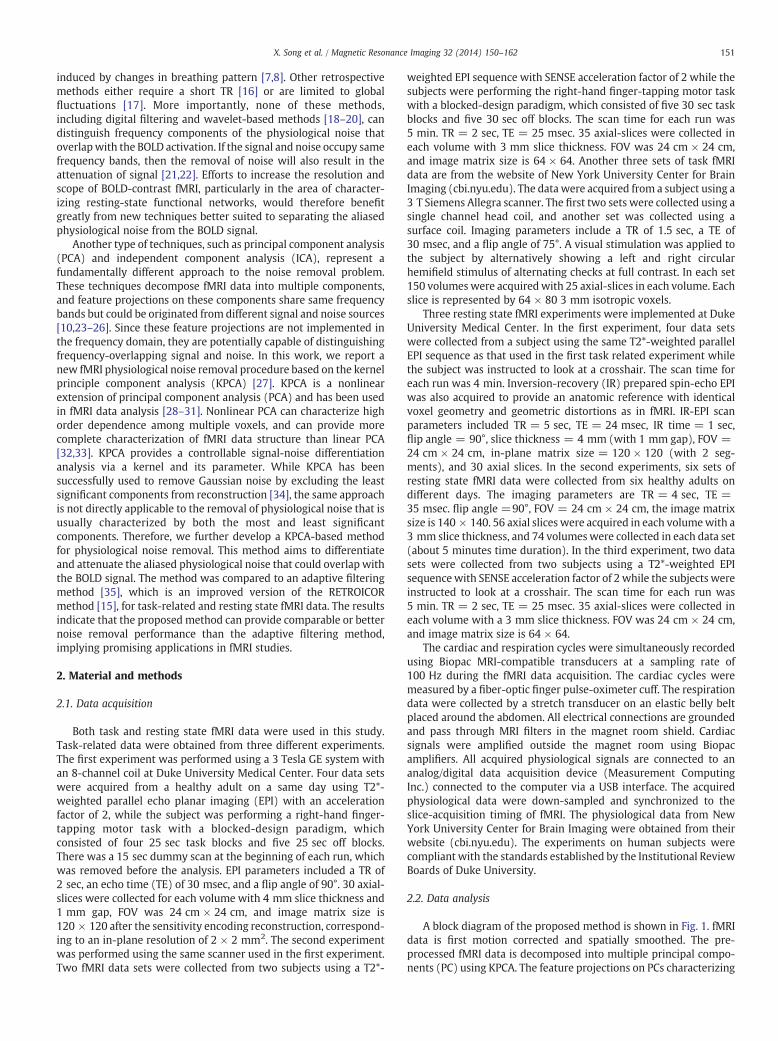
A block diagram of the proposed method is shown in Fig. 1. fMRIdata is first motion corrected and spatially smoothed. The pre-processed fMRI data is decomposed into multiple principal compo-nents (PC) using KPCA. The feature projections on PCs characterizing
Fig. 1. The block diagram of the proposed method.
152 X. Song et al. / Magnetic Resonance Imaging 32 (2014) 150–162
significant physiological variations are identified to locate frequen-cies of aliased physiological cycles, as indicated by simultaneouslyrecorded physiological data. The identified feature projections arefiltered by digital filters designed to attenuate the power at thesefrequencies. Finally KPCA reconstruction is implemented to obtainthe denoised data for the subsequent analysis.
2.2.1. PreprocessingAll fMRI data were first registered using a 2-D rigid body
registration method [36] as part of FSL tools [37] to remove smallhead motion artifacts. Then the data were detrended to remove lowfrequency drift and spatially smoothed with a Gaussian kernel(FWHM = 2 mm) using in-house Matlab programs. The restingstate data were low-pass filtered at the cut-off frequency of 0.1 Hz toremove high-frequency signal variations from the slowly-varyingsignal fluctuations of interest in resting state. All data werenormalized to zero mean and unit variance.
2.2.2. KPCA decompositionKPCA introduces nonlinearity into PCA through a kernel that
implicitly projects the input to a higher dimensional feature space[27]. A linear PCA performed in the feature space is equivalent to anonlinear PCA in the input space. Given M voxels sampled at T timepoints, we may form M T-dimensional vectors for spatial analysis, orT M-dimensional vectors for temporal analysis [24]. In this work, thetemporal analysis is used and each vector is represented asxi ∈ RM, i = 1, 2, ⋯, T. The PCs are obtained by computing eigen-values λ N 0 and eigenvectors V satisfying:
λV ¼ 1T
XT
i¼1
Φ xið Þ �Vh iΦ xið Þ; ð1Þ
where Φ is a nonlinear mapping from RM to a higher dimensionalfeature space F and ⟨ ⋅ ⟩ is the inner product operator. Because V =
span(Φ(xi) : i = 1, ⋯, T), we have V ¼XT
i¼1
αΦ xið Þ. If we define a
T × T matrix K with each entry as Ki,j = ⟨Φ(xi) ⋅ Φ(xj)⟩ and replace
the inner product in each entry with a kernel k(xi,xj), the eigenproblem becomes λα = Kα, where α = (α1,α2, ⋯,αT) '. After com-puting the single value decomposition on K, the feature projectionon the kth PC in F can be obtained by:
Vk⋅Φ xð Þ
D E¼
XT
i¼1
αki Φ xið Þ⋅Φ xð Þh i; ð2Þ
where Vk is the kth eigenvector in F.
2.2.3. Kernel evaluationIt is not clear howmuch separation between the BOLD signal and
physiological noise could be achieved by KPCA. The KPCA’s capability
relies on the kernel it uses. Different kernels and parameters willprovide distinct performances. The selection of kernels and param-eters has been discussed for support vector machine-based applica-tions [38] but rarely addressed for KPCA-based applications. In thiswork, two widely used kernels, the polynomial and radial basisfunction (RBF) kernels, as defined in Eq. (3), were examined withdifferent parameters regarding their performance in separating thephysiological noise and BOLD signal.
RBF kernel : k x;xið Þ ¼ e−jjx−xijj2
2σ2
Polynomial kernel : k x;xið Þ ¼ x;xih i þ 1ð Þp;ð3Þ
where σ is the RBF kernel width, ⟨x,xi⟩ is the inner product of vectorsx and xi, and p is the polynomial kernel order. Given a kernel and itsparameter, fMRI data is decomposed into multiple PCs using KPCA.Themutual information (MI) between the feature projection on eachPC and the expected haemodynamic response, and the MI betweenthe feature projection on the PC and the synchronized cardiac andrespiration cycles were calculated. Since projections showing highMI with the haemodynamic response are expected to have low MIwith the cardiac and respiratory recording, an index S was proposedto measure the separation performance as defined in (4).
SPHYS ¼ 1N
XN
k¼1
1−e− I BOLD kð Þ−I PHYS kð Þj j
; ð4Þ
where N is the number of PCs, IBOLD(k) is the MI between the featureprojection on the kth PC and the canonical haemodynamic responsefunction in task-related fMRI studies, and IPHYS(k) is the MI betweenthe projection on the kth PC and synchronized cardiac or respiratoryfluctuations, i.e., ICARD(k) or IRESP(k), which corresponds to SCARD orSRESP. If the feature projection on the kth PC has a high dependence onthe expected haemodynamic response but low dependence on thephysiological noise, or vice versa, then |IBOLD(k) − IPHYS(k)| isrelatively large and indicates a good separation between the BOLDsignal and noise. 1−e− I BOLD kð Þ−I PHYS kð Þj j is used to map this differenceto a range between 0 and 1, and a large |IBOLD(k) − IPHYS(k)| valueresults in a value of 1−e− I BOLD kð Þ−I PHYS kð Þj j close to 1. The final S indexis an average of all 1−e− I BOLD kð Þ−I PHYS kð Þj j values calculated fromthe feature projections on N PCs. Therefore, a better signal-noises e p a r a t i o n r e s u l t s i n a h i g h e r S v a l u e . S i n c e0≤1−e− I BOLD kð Þ−I PHYS kð Þj j≤1, the S value is also between 0 and 1. Forresting state studies, there is no experimental paradigm, and wepropose a different way to estimate IBOLD(k). First a seed is selectedwithin a functional network of interest, and the average time courseof the seed is used as the expected haemodynamic response tocompute IBOLD(k). Although it is possible that the seed is contam-inated by the physiological noise, the S value can provide a reliableevaluation of the separation performance because a kernel that cansufficiently separate the signal and noise to different PCs willgenerate large |IBOLD(k) − IPHYS(k)| values, leading to large S values.
Multiple data sets were used to identify a kernel and itsparameter that outperform the others in terms of the signal-noiseseparation performance measured by Eq. (4). Due to the non-stationary nature of fMRI, the data collected from different subjects,or a same subject but at a different timemay have very distinct signaland noise characteristics. Consequently, S values from different datasets are not directly comparable although they could be obtainedusing a same kernel and parameter, and only those computed from asame dataset with different kernels and parameters are comparable.To remove the effects from the non-stationarity, S values computedfrom each data set are normalized against the maximum S valuefrom the same data set using the two kernels. Meanwhile, the
153X. Song et al. / Magnetic Resonance Imaging 32 (2014) 150–162
difference between S values induced by different kernels andparameters using the same data set is preserved. After thenormalization, the S values from all data sets are comparable andaveraged together to increase the statistical power of the analysis.The kernel evaluation is not part of the block diagram as shown inFig. 1. It is implemented offline to provide guidance on the selectionof a kernel function and its parameter for KPCA decomposition.
2.2.4. Component analysis and reconstructionThe KPCA-based noise removal is a dimensionality reduction
problem that can be used to reveal low-dimensional representationsof a data set and to reflect its underlying degrees of freedom. Inexisting KPCA-based approaches, the least significant PCs aresupposed to characterize the noise and excluded from the recon-struction [31,34]. This might not be suitable for the physiologicalnoise removal because the physiological noise could be at a similar orhigher intensity level than BOLD signals [39,40]. Therefore, the noisecould be captured by the most significant PCs. Prior informationabout the physiological noise is needed in order to identify PCscharacterizing the noise, and is extracted from the synchronizedphysiological cycles.
The spectra of the synchronized physiological cycles are firstcalculated, and frequencies of interest (FOIs) showing peak power ofthe aliased cardiac and respiratory cycles are automatically detectedand recorded. In our preliminary study [29], the spectrum of eachfeature projectionwas examined at FOIs to identify PCs capturing thegreatest power of the noise. In this work, a more efficient wayproposed by using the frequency information and the MI betweenthe feature projections and physiological recording and expectedBOLD signal. A set of feature projections are identified if they (i)exhibit high ICARD and IRESP but low IBOLD values, and (ii) havesignificant power at the FOIs. The analysis starts with a ranking offeature projections in terms of ICARD and IRESP, respectively. Since itwas found that usually three to five feature projections showingmuch larger IBOLD values than other feature projections, in therankings of ICARD and IRESP, feature projections that are among thetop three showing the highest IBOLD are removed. The remainedprojections are examined at the FOIs. In each remained projection,the power at each FOI is estimated by summarizing the power of theclosest frequency point to the FOI and the power of the twoneighboring (one lower, one higher) frequency points. If the powerat the FOI is greater than 0.5 times the average of power spectrum,then a finite impulse response band-stop filter is designed toattenuate the noise components at this FOI. Since most featureprojections are not significant in terms of both BOLD signal andphysiological noise, it might not be necessary to analyze eachprojection, and only those with ICARD or IRESP values greater than theaverage of ICARD or IRESP will be examined and filtered. This improvesthe computational efficiency without considerably affecting thenoise removal performance.
KPCA reconstruction is not so straightforward as with linear PCA[34,41]. None of existing methods can provide a perfect reconstruc-tion. In our work, the method proposed by Kwok was used [41]. Itestimates the reconstructed data by utilizing distance constraints ininput and feature spaces derived by the idea of multidimensionalscaling (MDS) [42]. MDS states that the pairwise distance of two datapoints in an input space is preserved after projecting the data to ahigh dimensional feature space. The MDS-based KPCA reconstruc-tion is an optimization problem that aims to minimize the differencebetween the pairwise distance of points in the input and highdimensional feature spaces.
2.2.5. Method evaluationQuantitative measures were used to evaluate the proposed
method based on a comparison study with an adaptive filtering
method [35], which was developed based on the widely usedRETROICOR method [15]. For task-related data, a contrast-to-noiseratio (CNR) measurement was computed to assess the denoisingperformance [43]. It is defined as:
CNR ¼ ΔS0:5 SEbase þ SEtaskð Þ ; ð5Þ
where ΔS is the change of signal intensity in response to a taskstimulation, SE is the standard error of intensity in baseline or taskstimulation period, and is defined as: SE = SD/M0.5, where SD is thestandard deviation of the average intensity during the baseline ortask period, and M is the number of images during the baseline ortask period. The CNR values should increase or maintain at the samelevel after removing the noise in regions where BOLD activationsappear during the stimulation, and to decrease in regions contam-inated by the physiological noise. Temporal standard deviation mapswere computed for the original and denoised data. For resting statedata, MI values between a seed and part of the default mode network(DMN) was compared between the data denoised by the twomethods. The MI between the synchronized physiological recordingand fMRI data before and after the noise removal was also compared.
3. Results
3.1. Task-related experiments
The two kernels described in Eq. (3) were first evaluated withdifferent parameters using four sets of fMRI data acquired from thefirst task-related experiment. In each data set, three slices thatcontain significant BOLD responses were selected for the evaluation.Since each slice across time forms an image sequence, we had a totalof twelve image sequences. For the polynomial kernel, the kernelorder p ranged from 1 to 16 with an interval of 1, where order 1corresponds to the linear discrimination. For the RBF kernel, thekernel width parameter σwas set from 0.1 to 100, with an interval of0.1 when 0.1 ≤ σ b 1, with an interval of 1 when 1 ≤ σ b 10, andwith an interval of 10when 10 ≤ σ ≤ 100. The average and standarddeviation (SD) of S values of the two kernels were calculated usingthe twelve image sequences, as shown in Fig. 2, where (a) and (b)are SCARD values as a function of p and σ, respectively, and (c) and (d)are SRESP values as a function of p and σ, respectively. When thepolynomial kernel was used, there is no significant differencebetween S values as a function of p, as shown in Fig. 2 (a) and (c).For the RBF kernel, there is a significant increase of SCARD and SRESPwhen 0.5 ≤ σ ≤ 10. When σ N 10, the S values are close to thoseobtained from the polynomial kernel.
To illustrate the signal-noise separation in individual featureprojections, stacked bars are used to represent the estimated IBOLD(blue), IRESP (light-green), and ICARD (red-brown) values of allfeature projections, as shown in Fig. 3, where (a) was obtained usingthe polynomial kernel with p = 3, and (b) was calculated by usingthe RBF kernel with σ = 10.0. Each stacked bar is corresponding to afeature projection, and the IBOLD, IRESP, ICARD values are representedby the lengths of associated color segments. It is expected thatfeature projections with large IBOLD values have small IRESP and ICARDvalues, which indicates a clear separation between the BOLD signaland physiological noise.
Since the RBF kernel provides a better signal-noise separation interms of the measurement defined in (4) when 0.5 ≤ σ ≤ 10, theRBF kernel was used with σ = 6.0 in the proposed method toprocess the task-related data. For comparison, the adaptive filteringmethod was implemented for the same data. After the processing,CNR values were computed for the original and denoised data, andnormalized between 0 and 1 based upon the maximum and
Fig. 2. The average and standard deviation of SCARD and SRESP values calculated as a function of the polynomial kernel order (a, c) and the RBF kernel width (b, d) using four sets ofdata acquired from the first task-related experiment.
154 X. Song et al. / Magnetic Resonance Imaging 32 (2014) 150–162
minimum CNR values calculated from the original and denoised datafrom the two methods. Fig. 4 (a)-(c) show a comparison of thenormalized CNR values in a representing slice for one run of the firsttask-related experiment. Fig. 4 (a) was obtained from the originaldata, (b) was calculated from the data processed by the proposedmethod, and (c) was from the data denoised by the adaptive filteringmethod. Note there are some voxels in regions not related to the taskshowing decreased CNR as indicated by the two arrows in (b). Asimilar decrease is observed in the adaptive filtering result in (c). Aslight decrease of CNR in the left motor cortex is also observed in (c),implying possible attenuation of real BOLD activation by theadaptive filtering method. Fig. 4 (d)–(f) are the temporal standarddeviation maps, where (d) was computed from the original data, (e)
ig. 3. The stacked bar representation of ICARD, IRESP, and IBOLD values of all PCs obtained from a set of fMRI data using (a) the third order polynomial kernel and (b) the RBF kerneith a kernel width σ = 10.
Fw
and (f) were from the results of the proposed and adaptive filteringmethods, respectively. The proposed method provides more atten-uation on the temporal standard deviation than the adaptive filteringmethod without sacrificing CNR in the motor cortex.
So far the data used to evaluate the proposed method is the samedata used to identify the kernel and its parameter. We furtherexamined the method with the same kernel and parameter usingdifferent data sets. These data were obtained from different subjectswithmotor and visual stimuli. In addition, they have different spatialand/or temporal resolution, time length, and were acquired fromdifferent scanners. Fig. 5 (a) is an EPI slice in a data set acquired fromthe second task-related experiment where a motor task stimulationwas used. (b)–(d) are the normalized CNRmaps overlaid on the slice
Fig. 4. (a)–(c) Single slice CNR maps of a task-related experiment calculated from (a) the original data, (b) the data denoised by the proposed method, and (c) the data processedusing the adaptive filtering method. The two arrows in (b) point to groups of voxels with decreased CNR. (d)–(f) Single slice temporal standard deviation maps obtained from (d)the original data, (e) the data denoised by the proposed method, and (f) the data smoothed using the adaptive filtering method.
155X. Song et al. / Magnetic Resonance Imaging 32 (2014) 150–162
calculated from the original data and the data denoised by using theproposed and adaptive filtering methods. Fig. 5 (e) is another EPIslice in a data set collected from the third task-related experimentwhere a visual hemifield stimulation was implemented. (f)–(h) arethe normalized CNR maps obtained from the original and denoiseddata. It might not be easy to visually identify the difference amongthese CNR maps. Table 1 shows the number of voxels withnormalized CNR values above 0.6 and below 0.3 before and afterthe noise removal for the heretofore used three task-related fMRIdata sets shown in Figs. 4 and 5.
We further calculated S values using the data sets from thesecond and third task-related experiments. Fig. 6 (a)–(d) are theaverage and SD of S values of the two kernels calculated using thedata sets from the second and third task-related experiments. In the
Fig. 5. (a) An individual slice from a data set in the second task-related experiment where afrom (b) the original data, (c) the data denoised by the proposed method, and (d) the datathe third task-related experiment where a visual attention stimulation was applied, (f)–(h)denoised by the proposed method, and (h) the data processed by the adaptive filtering m
second task-related experiment, five slices showing BOLD activationover time in the motor cortex were identified in each data set, andtotally ten image sequences were used to calculate the S values. Inthe data sets from the third experiment, 15 image sequences wereused to calculate S values with five image sequences from each dataset showing BOLD activation in the primary visual cortex. It can beseen from Figs. 2 and 6 that the curves obtained using the polynomialkernel exhibit a similar pattern, and those obtained using the RBFkernel show another similar pattern.
3.2. Resting state experiments
The proposed method was also evaluated using the resting statedata. In the data from the first resting state experiment, a 3 × 3
motor task was performed, (b)–(d) are the CNR maps overlaid on this slice calculatedsmoothed using the adaptive filtering method. (e) An individual slice from a data set inare the CNRmaps overlaid on the slice obtained from (f) the original data, (g) the dataethod.
Table 1The number of voxels with high (N0.6) and low (b0.3) normalized CNR values before and after noise removal. The corresponding CNR maps are shown in Figs. 4 and 5.
Data set #1 Data set #2 Data set #3
High CNR (N0.6) Low CNR (b0.3) High CNR (N0.6) Low CNR (b0.3) High CNR (N0.6) Low CNR (b0.3)
156 X. Song et al. / Magnetic Resonance Imaging 32 (2014) 150–162
voxels seed was manually selected in the posterior cingulate cortex(PCC) region that is part of the DMN. The average time course of thisseed was used as an expected haemodynamic response, from whichIBOLD was estimated. Fig. 7 shows the average and SD of S values ofthe two kernels estimated using the four sets of resting state data. Ineach data set, three image sequences corresponding to three slicescontaining DMN regions were used to calculate S values, and thereare total 12 image sequences used to obtain the results in Fig. 7. MostS values are at a similar level, but we may see an increase in averagevalue from the RBF kernel when 0.5 ≤ σ ≤ 10. Like the noiseremoval of task-related data, we also chose the RBF kernel with σ =6.0 for the resting state physiological noise removal.
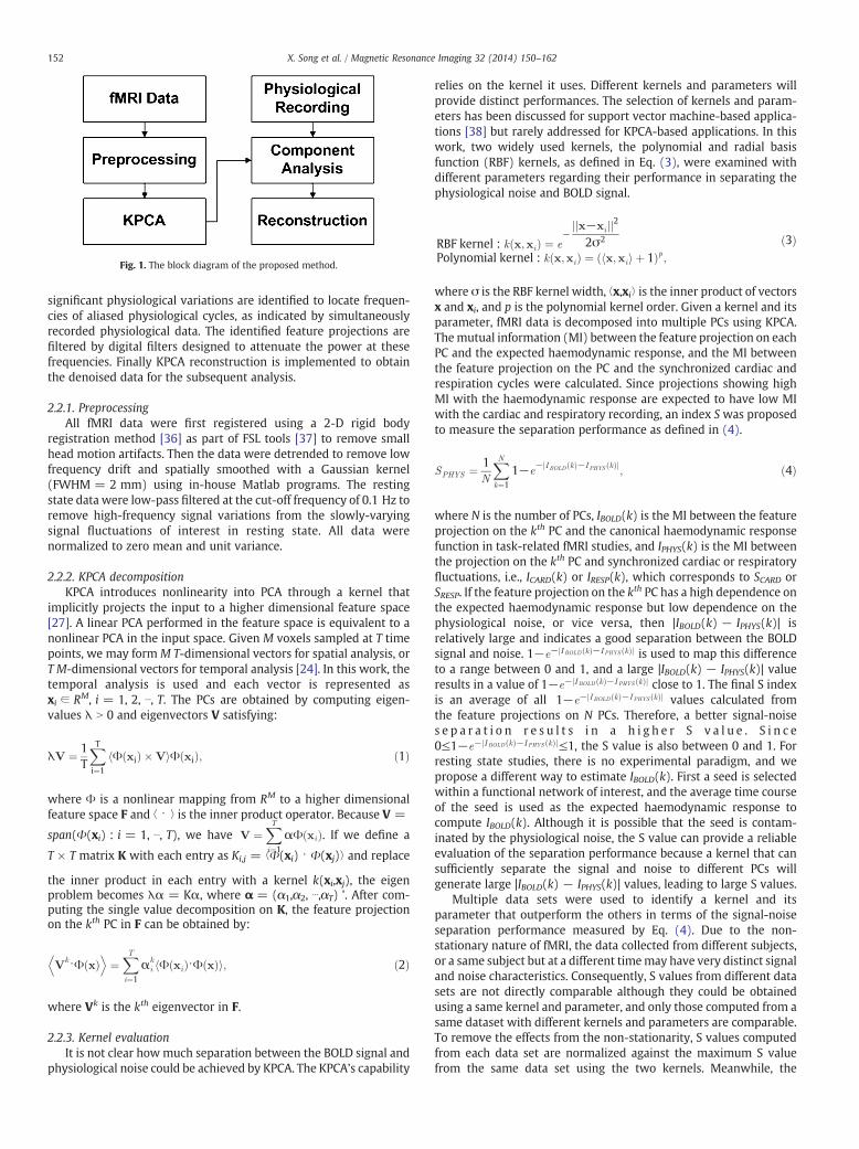
MI values were calculated between the seed’s and all voxels’ timecourses using the original data, the data processed by the proposedand adaptive filtering methods. These MI values were normalized tothe maximum MI value calculated from the original and denoiseddata, and overlaid on the corresponding image slice as shown inFig. 8 (a)–(c), where the encircled region in (a) is the seed based onwhich the S values in Fig. 7 were obtained. Fig. 8 (b) and (c) indicatethat the proposed and adaptive filtering methods can increase thenumber of voxels showing high MI to the seed in PCC, medialprefrontal cortex (mPFC), and lateral parietal cortex (LPC). In orderto examine the physiological noise distribution in this slice beforeand after the noise removal, the MI values between the fMRI data
ig. 6. The average and standard deviation of SCARD and SRESP values calculated as a function of the polynomial kernel order (a, c) and the RBF kernel width (b, d) using two data
F sets collected from the second task-related fMRI experiment, and three data sets from the third task-related fMRI experiment.
and the synchronized physiological cycles were computed andnormalized to the maximum MI value computed from the originaland denoised data, as shown in Fig. 8 (d)–(i), where a MI value closeto 1 means a high similarity between the data and noise. Specifically,Fig. 8 (d)–(f) are MI maps between the synchronized cardiacrecording and (d) original data, (e) data processed by the proposedmethod, and (f) the data smoothed by the adaptive filtering method.(g)–(i) are MI maps between the synchronized respiration recordingand (g) original data, (h) data processed by the proposed method,and (i) the data denoised by the adaptive filtering method. It isobserved that both methods can attenuate the dependence of fMRIdata on the physiological fluctuations.
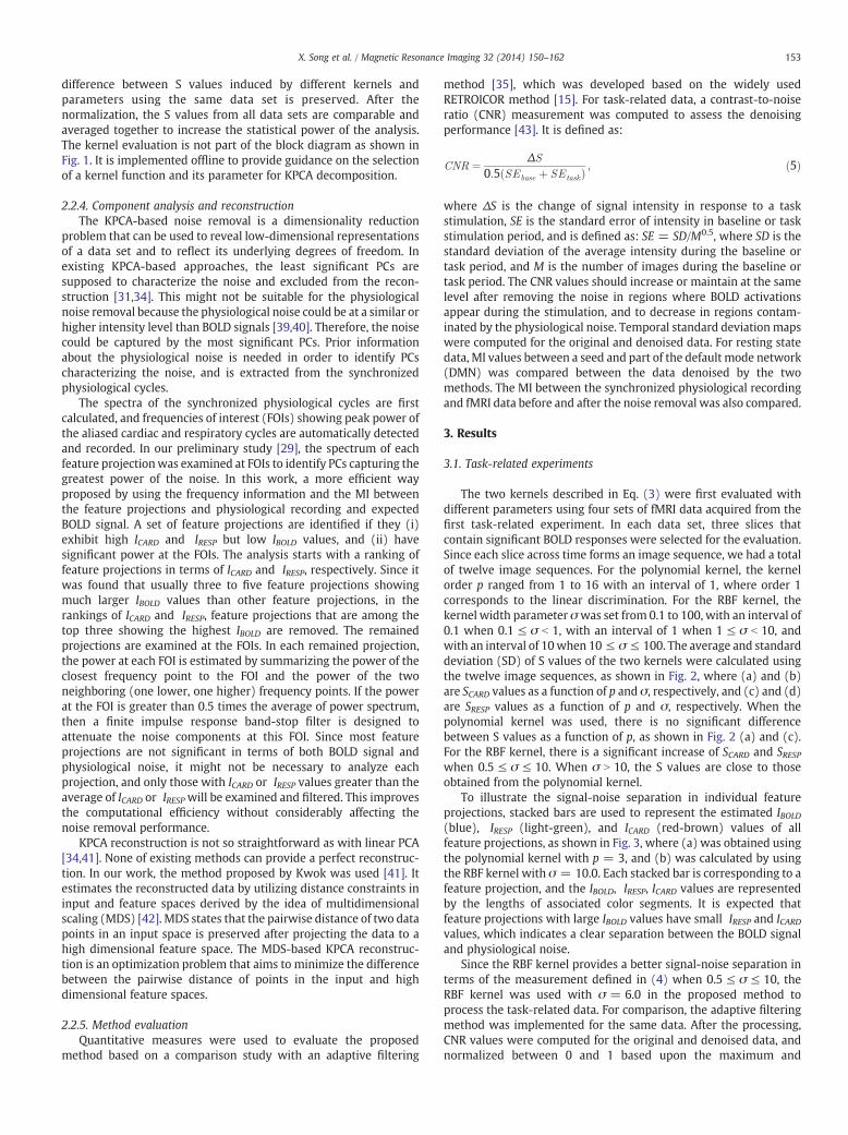
The same kernel and parameter were applied to the other datasets collected from the second and third resting state experiments.Fig. 9 (a) shows an individual slice in a data set from the secondresting state experiment. (b)–(d) are the MI maps between a 3 × 3voxels seed in PCC and all voxels’ time courses overlaid on the sliceusing (b) the original data, (c) the data denoised by the proposedmethod, and (d) the data processed by the adaptive filteringmethod.Fig. 9 (e) is an individual slice from another set of data collected fromthe third resting state experiment. (f)–(h) show the same type of MImaps as (b)–(d) using this data. The S values calculated using thedata sets from the second and third resting state experiments areshown in Fig. 10 (a)–(d). There are six sets of data from the second
Fig. 7. The average and standard deviation of SCARD and SRESP values calculated as a function of the polynomial kernel order (a, c) and the RBF kernel width (b, d) using four sets ofMRI data collected from the first resting state fMRI experiment.
157X. Song et al. / Magnetic Resonance Imaging 32 (2014) 150–162
resting state experiment, and eighteen image sequences were usedwith three image sequences from each data set. There are two datasets from the third resting state experiment, with three imagesequences from each data set. The average and SD of S values exhibita similar pattern as those in Fig. 8. This implies that the proposedsignal noise separation measurement is independent of experimentparadigm, subjects, spatial and temporal resolution, and time lengthof experiments, and the identified kernel and its optimal parameterrange are applicable to the physiological noise removal in differentfMRI experiments.
4. Discussion
MI was used in this work to reveal high order dependenciesbetween the KPCA feature projections and expected haemodynamicresponses or synchronized cardiac/respiratory fluctuations. It is noteasy to accurately estimate MI values, and two MI estimationmethods were examined in this study [44,45]. It was found that thetwo methods generate slightly different MI estimates but providealmost same patterns for S values as a function of different kernelparameters. Therefore, they may be used to estimate relativeincreases/decreases of MI or MI-based measures, such as theproposed S index. The method proposed by Darbellay et al. wasfinally used for this study because it is computationally moreefficient [45]. The MI measures in equation (4) could be replaced bythe absolute value of Pearson's correlation coefficient, which cancharacterize the second order dependencies between feature pro-jections and signal/noise. A comparison between the MI- andcorrelation-based S indices was performed using all task-relatedfMRI experimental data presented in this work, and part of results isshown in Fig. 11, where (a) and (b) are S values as functions of theRBF kernel width obtained using the two MI estimation methods,and (c) was obtained by using the correlation coefficient in
f
equation (4). The variation of S values in (a) and (b) are quite similarto each other except for their values after the normalization. The Svalues obtained using the correlation coefficient also show anincrease when 0.5 ≤ σ ≤ 10, but the increase is not so significant asthose in (a) and (b) calculated using MI. A possible reason of thisdifference is that MI can provide a more complete characterization ofdependencies between the feature projections and haemodynamicresponses or synchronized cardiac/respiratory cycles than thecorrelation coefficient.
Under the task stimulation, there is no significant difference in Svalues when different polynomial kernel order is used, as shown inFig. 2 (a), (c), Fig. 6 (a), and (c). When the RBF kernel is used, theaverage S values are usually less than those of the polynomial kernelif σ b 0.5, as shown in Fig. 2 (b), (d), Fig. 6 (b), and (d). However,when 0.5 ≤ σ ≤ 10, the average S values are greater than thoseobtained from the polynomial kernel. When σ N 10, the average Svalues are close to those calculated from the polynomial kernel. Asimilar observation was made from the S values computed from theresting state experiments, as shown in Figs. 7 and 10. When thepolynomial kernel is used with p = 1, the KPCA becomes the linearPCA. When the RBF kernel is used with a large kernel width, theKPCA is close to the linear PCA. Figs. 2, 6, 7, and 10 also indicate thatthe nonlinear KPCA can provide better signal-noise differentiationthan the linear PCA if the kernel and its parameter are properlychosen. For instance, the S values shown in these figures tell us thatthe RBF kernel with 0.5 ≤ σ ≤ 10 may be used. This observation isreasonable from the machine learning aspect. When the RBF kernelwidth is small (i.e., σ b 0.5), the feature space distance betweendifferent feature points is close to zero, and PCA analysis in thefeature space becomes unstable and meaningless [46]. On the otherhand, if the RBF kernel width is large (i.e., σ N 10), KPCA is close tothe conventional linear PCA, which is not sufficient to characterizethe nonlinear fMRI data structure. A moderate kernel width (i.e.,
Fig. 8. Mutual information (MI) based evaluation of resting state fMRI physiological noise removal. The MI values were normalized to the maximum MI computed from theoriginal and denoised fMRI data, and overlaid on an image slice that covers part of the DMN. (a)–(c) are MI maps between a seed (encircled region in (a)) in the PCC area and (a)the original data, (b) the data denoised by the proposedmethod, and (c) the data processed using the adaptive filteringmethod. AMI value close to 1means a high dependence onthe seed. (d)–(f) are MI maps between the synchronized cardiac recording and (d) the original data, the data denoised by (e) the proposed method, and (f) the adaptive filteringmethod. (g)–(i) are MI maps between the synchronized respiration recording and the fMRI data in a same order as (d)–(f). The regions pointed by arrows in (d) partially overlapwith the DMN but can be attenuated by the proposed and adaptive filtering methods without affecting the identification of voxels showing high MI with the seed.
158 X. Song et al. / Magnetic Resonance Imaging 32 (2014) 150–162
0.5 ≤ σ ≤ 10) not only can introduce sufficient nonlinearity tocharacterize fMRI data structure, but also can avoid the unstable PCAcomputation in the feature space. A further examination of Figs. 2, 6,7, and 10 indicates that when 0.5 ≤ σ ≤ 2, the standard deviation ofS is relative large in some data sets, implying an inconsistent signal-noise separation performance. The reason of this inconsistency isthat these kernel width values are still small and cannot guarantee toprovide reliable PCA analysis for all data sets. They may yield morescattering of the feature variance into the PCs, resulting in asignificant number of PCs showing either high ICARD, IRESP, or highIBOLD values, which are not expected for the analysis. An expectedKPCA decomposition generates only a few PCs that are significant interms of either BOLD signal or the physiological noise. Therefore, inorder to obtain a reliable decomposition, we suggest setting the RBFkernel width between 2 and 10. In the experiments, we examined akernel width of 6.0 for the noise removal of both task-related andresting state data.
The IBOLD, ICARD, and IRESP values of all PCs shown in Fig. 3 (a) wereobtained after the KPCA decomposition of a task-related fMRI timeseries using the third order polynomial kernel. The third orderpolynomial kernel has been widely used in various pattern
recognition tasks because it could provide sufficient nonlinearitywithout a significant increase of computational load. From the lengthof each color segment in the stacked bar, it was observed that themost significant PC computed by using this kernel shows asignificant dependence on the BOLD signal. It also has an apparentdependence on the cardiac cycles, and little dependence on therespiration. Within the first ten most significant PCs, there are twoPCs showing significant dependence on the physiological noise andlittle dependence on the BOLD signal. From the 11th significant PC tothe least significant PC, there are a small number of PCs showingsignificant dependence on the BOLD activation and little dependenceon the physiological noise, or the opposite situation. Most other PCsexhibit either similar or little dependence on both the BOLD signaland physiological noise. When the RBF kernel with σ = 10was usedfor the same data, the first most significant PC shows a significantdependence on the BOLD signal, but little dependence on eithercardiac or respiration cycles, as shown in Fig. 3 (b). Within the firstten most significant PCs, there is one PC showing significantdependence on the physiological noise and little dependence onthe BOLD signal. If we compare the PCs from the 11th significant tothe least significant to those obtained from the third-order
Fig. 9.Mutual information (MI) between a seed in PCC and the original and denoised fMRI data calculated from two sets of resting state data. TheMI values were normalized to themaximum MI computed from the original and denoised fMRI data in each data set, and overlaid on the corresponding slice that covers the seed region. (a) shows an individualslice from one data set where the seed was selected. (b) is the MI map calculated using the original data, (c) is the MI map computed using the data denoised by the proposedmethod, and (d) is from the data processed by the adaptive filtering method. (e) is an individual slice from the other data set where the seed was selected in PCC. (f)–(h) are theMI maps following the same order as (b)–(d) calculated using the original and denoised slice in this data set.
159X. Song et al. / Magnetic Resonance Imaging 32 (2014) 150–162
polynomial kernel, we may find that the polynomial kernelgenerates more PCs showing apparent dependence on the BOLDactivation than the RBF kernel. These observations indicate that theRBF kernel with σ = 10 has a better characterization of the BOLDsignal and physiological noise than the third order polynomial
Fig. 10. The average and standard deviation of SCARD and SRESP values calculated as a functisets acquired from the second resting state fMRI experiment, and two data sets from the
kernel, and provides a better signal-noise separation for this data.None of existing techniques, such as ICA, PCA, and KPCA, cancompletely separate the BOLD signal and physiological noise. Butthey can facilitate the identification of the majority of physiologicalfluctuations. As long as KPCA can provide a reasonable decomposi-
on of the polynomial kernel order (a, c) and the RBF kernel width (b, d) using six datathird resting state fMRI experiment.
Fig. 11. The average and standard deviation of SCARD values calculated as a function of the RBF kernel width based on all task-related fMRI data presented in this work. (a) and (b)were obtained by using the MI estimation methods proposed by Darbellay et al. [45], and Beirlant et al. [44], respectively. (c) was obtained by replacing MI with the absolutevalues of Pearson's correlation coefficient in the calculation of S values.
160 X. Song et al. / Magnetic Resonance Imaging 32 (2014) 150–162
tion with a properly selected kernel and parameter, the mostsignificant part the physiological noise can be characterized by PCsthat are different from those characterizing BOLD signal, and afrequency analysis performed on feature projections of these PCs canbetter differentiate the physiological noise than the conventionalfrequency analysis performed on the original fMRI data.
There are many methods that can easily reduce the temporalstandard deviation of voxels. But as a consequence, CNR of trulyactivated brain voxels is also attenuated. From the results in Fig. 4, itis interesting to find that the proposed method can provide a moresignificant attenuation of the temporal standard deviation than theadaptive filtering without sacrificing CNR of truly activated brainvoxels. This implies that the decreased standard deviation likelyrepresents the physiological fluctuations, and the BOLD CNR can bemaintained or enhanced by the proposed method. This is furtherverified by the results from the other two data sets collected fromdifferent subjects, different experiments with different tasks, asshown in Fig. 5. The numerical results in Table 1 were computed tohelp the comparison of CNR maps shown in Figs. 4 and 5. Comparedto the number of voxels showing high and low CNR values in theoriginal data, the data denoised by the proposed method have asimilar or greater number of high CNR voxels, and more low CNRvoxels. There are less high CNR voxels in the data processed by theadaptive filtering method. This indicates that the attenuation of thephysiological noise also lead to the reduction of BOLD signal whenthe adaptive filtering method was used. This also implies that part ofBOLD frequencies overlap with the aliased physiological noise, andthe proposed method can differentiate the frequency-overlappingsignal and noise.
The evaluation of the denoising performance on resting statedata is challenging because it is difficult to judge if there would be
greater or fewer functionally connected regions after the proces-sing. There are two types of errors caused by the physiological noisein resting state studies [47]. One is the false positive when there isno functional connection but the dependence between noisecomponents is significant enough with respect to a predefinedthreshold. The other is false negative when the true functionalconnection is obscured by the physiological noise and cannot bedetected. The first type of error leads to more voxels showingsignificant dependence to the seed, and the noise removal shouldreduce the number of connected voxels. The second type of errorresults in less voxels connected to the seed, and the noise removalshould increase the connected area. In practice, it is difficult toknow if the number of voxels connected to the seed should increaseor decrease after the noise removal. But according to the existingknowledge about the spatial distribution of physiological noise, andresults from previous studies, it is possible to determine if the noiseremoval is effective or not.
DMN is widely used to evaluate the physiological noise effect inresting state fMRI studies. In this study, MI was computed to identifyDMN based on a seed in PCC as shown in Fig. 8 (a). Regions with redcolor indicate significant connections with the seed. Since all MIvalues were normalized against a same base, the comparison of MImaps in each row of Fig. 8 are meaningful. For the data shown inFig. 8, both the proposed and adaptive filtering methods increase thenumber of functionally connected voxels in PCC, mPFC, and LPC, asshown in Fig. 8 (b) and (c). In addition, the proposed processingresults in more connected voxels than the adaptive filtering method.It was also observed from Fig. 8 (b) and (c) that some regions thatare not considered as part of DMN show increased MI with the seedregion. In order to check the significance of these increases, wemanually selected four DMN regions covering PCC (288 voxels),
161X. Song et al. / Magnetic Resonance Imaging 32 (2014) 150–162
mPFC (180 voxels), left and right LPC (321 voxels), and calculatedthe ratio between the average MI within these regions and theaverage MI of all other regions (3372 voxels). The ratio is 1.18 in theoriginal data, 1.23 after the adaptive filtering, and 1.33 after theproposed processing. Therefore, the increases of MI in DMN regionsare more significant than those in other regions. An examination ofthe noise distribution before and after the noise removal in Fig. 8(d)–(i) may give us more information about the performance of twomethods. It was observed that both methods can considerablyattenuate the dependence of the fMRI data to the synchronizedphysiological cycles, implying that the methods can effectivelyreduce the physiological noise. It was also observed that there ismore attenuation to the respiration-induced noise than to thecardiac-induced noise, as shown in Fig. 8 (e)–(f), and (h)–(i). Thereare several regions indicated by arrows in Fig. 8 (d). These regionspartially overlap with the DMN, and show significant dependence onthe synchronized cardiac cycles. Both methods can reduce thecardiac noise in these regions, and facilitate the identification ofmore functionally connected voxels, as indicated by the voxels thatshow low MI to the seed in Fig. 8 (a), but show high MI values inFig. 8 (b) and (c). The performance of the proposed method can befurther verified by the identified DMN from two different data setsshown in Fig. 9, where each row starts with an EPI image slice onwhich the denoising was performed. Fig. 9 (b) and (f) are thenormalizedMI maps between a seed in PCC and the original data. (c)and (g) are the normalized MI maps between the seed and the datadenoised by the proposedmethod. (d) and (e) are the normalizedMImaps between the seed and the data processed by the adaptivefiltering method. Both the proposed and adaptive filtering ap-proaches can increase the MI with the seed in PCC, mPFC, and LPCregions, and the results from the proposed method show higher MIvalues in these regions than those from the adaptive filteringmethod.
The proposed KPCA based method also has limitations. First, likeICA- or PCA-basedmethods, it is not guaranteed that signal and noisecan be completely separated into different components. Secondly,the frequency analysis is implemented on each PC across the entirerecording period, and short time changes of noise frequencies maynot be sufficiently characterized. The simultaneous physiologicalrecording is not mandatory for the study. Approaches that use eitherICA components [48,49], or data from a noise region in white matteror ventricle, or regions around large vessels can also be used toprovide an estimation of the physiological noise [50].
5. Conclusion
The challenge of fMRI physiological noise removal was addressedin this study based on a KPCA based physiological noise removalmethod. The polynomial and RBF kernels were examined for theKPCA using a signal-noise separation measurement that wasproposed to evaluate the kernels’ performance in differentiatingthe physiological noise and BOLD signal. Experimental study showsthat the RBF kernel is a better choice for the separation of thephysiological noise when the kernel width is properly set. Based onthe RBF kernel, the KPCA-based physiological noise removal methodwas developed and evaluated using both task-related and restingstate fMRI data acquired from multiple human subjects. A compar-ison study with an adaptive filtering method was also performed.The results indicate that the proposed method can providecomparable or better physiological noise removal performancethan the adaptive filtering method. Particularly, a major advantageof the proposed method is its potential capability to differentiatefrequency-overlapping signal and noise. This distinguishes it frommost existing methods that use adaptive filtering and/or regression
models to smooth the data, which could simultaneously attenuatethe noise and signal.
Acknowledgments
This research was partially supported by NIH R01-NS074045grant (to N.-K. Chen).
References
[1] Ugurbil K, Hu X, ChenW, Zhu X, Kim SG, Georgopoulos A. Functional mapping inthe human brain using high magnetic fields. Philos Trans R Soc Lond B Biol Sci1999;354:1195–213.
[2] Kruger G, Glover GH. Physiological noise in oxygenation-sensitive magneticresonance imaging. Magn Reson Med 2001;46:631–7.
[3] Di Salle F, Esposito F, Elefante A, Scarabino T, Volpicelli A, Cirillo S, et al. High fieldfunctional MRI. Eur J Radiol 2003;48:138–45.
[4] Voss HU, Zevin JD, McCandliss BD. Functional MR imaging at 3.0 T versus 1.5 T: apractical review. Neuroimaging Clin N Am 2006;16:285–97.
[5] Biswal B, Yetkin FZ, Haughton V, Haughton VM, Hyde JS. Functional connectivityin the motor cortex of resting human brain using echo-planar MRI. Magn ResonMed 1995;34(4):537–41.
[6] Fox M, Snyder AZ, Vincent JL, Corbetta M, Van Essen DC, Raichle ME. The humanbrain is intrinsically organized into dynamic, anticorrelated functional networks.Proc Natl Acad Sci U S A 2005;102:9673–8.
[7] Birn RM, Diamond JB, SmithMA, Bandettini PA. Separating respiratory-variation-related fluctuations from neuronal-activity-related fluctuations in fMRI. Neuro-Image 2006;31:1536–48.
[8] Birn RM, Murphy K, Bandettini PA. The effect of respiration variations onindependent component analysis results of resting state functional connectivity.Hum Brain Mapp 2008;29:740–50.
[9] Broyd SJ, Demanuele C, Debener S, Helps SK, James CJ, Sonuga-Barke EJ. Default-mode brain dysfunction in mental disorders: a systematic review. NeurosciBiobehav Rev 2009;33:279–96.
[10] Zollei L, Panych L, Grimson E, Wells III WM. Exploratory identification of cardiacnoise in fMRI images. Proc. International Society and Conference on MedicalImage Computing and Computer-Assisted Intervention; 2003.
[12] Stenger VA, Peltier S, Boada FE, Noll DC. 3D spiral cardiac/respiratory orderedfMRI data acquisition at 3 Tesla. Magn Reson Med 1999;41:983–91.
[13] Hu X, Kim SG. Reduction of signal fluctuation in functional MRI using navigatorechoes. Magn Reson Med 1994;31:495–503.
[14] Hu X, Le TH, Parrish T, Erhard P. Retrospective estimation and correction ofphysiological fluctuation in functional MRI. Magn Reson Med 1995;34:201–12.
[15] Glover GH, Li TQ, Ress D. Image-based method for retrospective correction ofphysiological motion effects in fMRI: RETROICOR. Magn Reson Med 2000;44:162–7.
[16] Wowk B, McIntyre MC, Saunders JK. k-Space detection and correction ofphysiological artifacts in fMRI. Magn Reson Med 1997;38:1029–34.
[17] Frank LR, Buxton RB, Wong EC. Estimation of respiration-induced noisefluctuations from undersampled multislice fMRI data. Magn Reson Med2001;45:635–44.
[18] Biswal B, DeYoe AE, Hyde JS. Reduction of physiological fluctuations in fMRIusing digital filters. Magn Reson Med 1996;35:107–13.
[19] Meyer FG. Wavelet-based estimation of a semiparametric generalized linearmodel of fMRI time-series. IEEE Trans Med Imaging 2003;22:315–22.
[20] Song X, Murphy M, Wyrwicz AM. Spatiotemporal denoising and clustering offMRI Data. Proc. IEEE International Conference on Image Processing; 2006.p. 2857–60.
[21] Harvey A, Pattinson K, Brooks J, Mayhew S, Jenkinson M, Wise R. Brainstemfunctional magnetic resonance imaging: disentangling signal from physiologicalnoise. J Magn Reson Imag 2008;28:1337–44.
[22] Beall E. Adaptive cyclic physiological noise modeling and correction in functionalMRI. J Neurosci Methods 2010;187:216–28.
[23] McKeown MJ, Makeig S, Brown GG, Jung TP, Kindermann SS, Bell AJ, et al.Analysis of fMRI data by blind separation into independent spatial components.Hum Brain Mapp 1998;6:160–88.
[24] Andersen AH, Gash DM, Avison MJ. Principal component analysis of the dynamicresponse measured by fMRI: a generalized linear systems framework. MagnReson Imaging 1999;17:795–815.
[25] Thomas CG, Harshman RA, Menon RS. Noise reduction in BOLD-based fMRI usingcomponent analysis. NeuroImage 2002;17:1521–37.
[26] Churchill W, Yourganov G, Spring R, Rasmussen M, Lee W, Ween E, et al.PHYCAA: data-driven measurement and removal of physiological noise in BOLDfMRI. NeuroImage 2012;59(2):1299–314.
[27] Schölkopf B, Smola A, Müller K. Nonlinear component analysis as a kerneleigenvalue problem. Neural Comput 1998;10:1299–319.
[28] Thirion B, Faugeras O. Dynamical components analysis of fMRI data throughkernel PCA. NeuroImage 2003;20:34–49.
162 X. Song et al. / Magnetic Resonance Imaging 32 (2014) 150–162
[29] Song X, Ji T, Wyrwicz A. Baseline drift and physiological noise removal in highfield fMRI data using kernel PCA. Proc. IEEE International Conference onAcoustics, Speech, and, Signal Processing; 2008. p. 441–4.
[30] López M, Ramírez J, Górriz J, Álvarez I, Salas-Gonzalez D, Segovia F, et al. SVM-based CAD system for early detection of the Alzheimer's disease using kernel PCAand LDA. Neurosci Lett 2009;464(3):233–8.
[31] Rasmussen P, Abrahamsen T, Madsen K, Hansen L. Nonlinear denoising andanalysis of neuroimages with kernel principal component analysis and pre-image estimation. NeuroImage 2012;60(3):1807–18.
[32] Friston K, Phillips J, Chawla D, Büchel C. Revealing interactions among brainsystems with nonlinear PCA. Hum Brain Mapp 1999;8:92–7.
[33] Friston K, Phillips J, Chawla D, Büchel C. Nonlinear PCA: characterizinginteractions between modes of brain activity. Philos Trans R Soc Lond B BiolSci 2000;355(1393):135–46.
[34] Mika S, Schölkopf B, Smola A, Miller K, Scholz M, Ratsch G. Kernel PCA and De-noising in Feature Spaces. Advances in Neural Information Processing Systems11. Cambridge, MA: MIT Press; 1999. p. 536–42.
[35] Deckers R, Gelderen P, Ries M, Barret O, Duyn J, Ikonomidou V, et al. An adaptivefilter for suppression of cardiac and respiratory noise in MRI time series data.NeuroImage 2006;33:1072–81.
[36] Jenkinson M, Bannister P, Brady J, Smith S. Improved optimisation for the robustand accurate linear registration and motion correction of brain images.NeuroImage 2002;17(2):825–41.
[37] Woolrich M, Jbabdi S, Patenaude B, Chappell M, Makni S, Behrens T, et al.Bayesian analysis of neuroimaging data in FSL. NeuroImage 2009;45:S173–86.
[38] Ben-Hur A, Ong CS, Sonnenburg S, Schölkopf B, Ratsch G. Support vectormachines and kernels for computational biology. PLoS Comput Biol 2008;4(10):1–10 [e1000173].
[39] Bandettini P, Wong E, Jesmanowicz A, Prost R, Cox R, Hinks R. MRI of humanbrain activation at 0.5 T, 1.5 T and 3.0 T: comparison of DR2 and functionalcontrast to noise ratio. Proc ISMRM 1994;1:434.
[40] Triantafyllou C, Hoge R, Krueger G, Wiggins C, Potthast A, Wiggins G, et al.Comparison of physiological noise at 1.5 T, 3 T and 7 T and optimization of fMRIacquisition parameters. NeuroImage 2005;26:243–2505.
[41] Kwok JT, Tsang IW. The pre-image problem in kernel methods. IEEE Trans NeuralNetw 2004;15:1517–25.
[42] Williams CKI. On a connection between kernel PCA andmetric multidimensionalscaling. Advances in Neural Information Processing Systems 13. Cambridge, MA:MIT Press; 2001. p. 675–81.
[43] Menon RS, Thomas CG, Gati JS. Investigation of BOLD contrast in fMRI usingmulti-shot EPI. NMR Biomed 1997;10:179–82.
[44] Beirlant J, Dudewicz E, Gyorfi L, Van der Meulen E. Nonparametric entropyestimation: an overview. Int J Math Stat Sci 1997;6(1):17–39.
[45] Darbellay G, Vajda I. Estimation of the information by an adaptive partitioning ofthe observation space. IEEE Trans Inf Theory 1999;45(4):1315–21.
[46] HoffmannH.KernelPCA, for novelty detection. PatternRecogn2007;40(3):863–74.[47] Chang C, Glover GH. Effects of model-based physiological noise correction on
default mode network anti-correlations and correlations. NeuroImage2009;47(4):1448–59.
[48] Beall E, Lowe M. Isolating physiologic noise sources with independentlydetermined spatial measures. NeuroImage 2007;37:1286–300.
[49] Perlbarg V, Bellec P, Anton JL, Pelegrini-Issac M, Doyon J, Benali H. CORSICA:correction of structured noise in fMRI by automatic identification of ICAcomponents. Magn Reson Imaging 2007;25:35–46.
[50] Behzadi Y, Testom K, Liau J, Liu T. A component based noise correction method(CompCor) for BOLD and perfusion based fMRI. NeuroImage 2007;37(1):90–101.