A kinetic study of the oligomerization of propene, butene ...

Univers

ity of

Cap

e Town

A KINETIC STUDY OF THE OLIGOHERIZATION OF PROPENE,

BUTENE AND VARIOUS HEXENES OVER SOLID PHOSPHORIC ACID

BY

DEAGHLAN HARTIN HcCLEAN

B. Sc. ( Eng) ( Cape Town)

Submitted to the University of Cape Town

in fulfilment of the requirements for the degree of

DOCTOR OF PHILOSOPHY

Department of Chemical Engineering

University of Cape Town

Rondebosch, Cape

South Africa

The copyright of this thesis vests in the author. No quotation from it or information derived from it is to be published without full acknowledgement of the source. The thesis is to be used for private study or non-commercial research purposes only.

Published by the University of Cape Town (UCT) in terms of the non-exclusive license granted to UCT by the author.

Univers

ity of

Cap

e Tow

n

i

ACKNORLEDGEHENTS

I would like to express my sincerest thanks to my supervisors, Professor

Cyril T O'Connor and to Dr Hasami Kojima for their guidance and

friendship during the course of this work.

I wish to thank Jack Fletcher, Hare Rautenbach, Rerner Schumann, Gordon

Reid and Antoinette Upton for their invaluable assistance and friendship

over the years.

The following people and Institutions are also gratefully acknowledged:

SASOL, Caltex and the Council for Scientific and Industrial Research

for financial and technical assistance. In particular Hr K Kriel

and Dr H Dry of SASOL;

Professor Brian Paddon of the Department of Chemical Engineering for

his perennial and enthusiastic assistance;

All on the technical staff particularly messrs A Barker and R

Senekal of the Chemical Engineering Rorkshop without whose

assistance this thesis would not have been possible;

The glassblower, Hr C Ledger, for his practical assistance and Hiss

B Rilliams for the mass spectroscopic analysis;

Hr T Classens for the use of his multi-parameter modelling program;

I Rould like to express special thanks to my wife, Helen, for her

untiring and dedicated help with the typing of the thesis.

ii

TO KY FATHER SEAKUS

iii

SYNOPSIS

The oligomerization of propane, butanes and hexenes over solid phosphoric

acid catalyst has been investigated using an internal recycle reactor, a

pulse micro-catalytic reactor and a fixed bed reactor.

The relative reactivities of the propane, butanes and hexane feeds were

examined in a pulse reactor. Mechanistic pathways, particularly for

propene and butene oligomerization, have been proposed. In the pulse

reactor at 1. 65 MPa and 473 K the alkenes oligomerized according to the

following order of decreasing reactivity: iso-butene, 2-methyl-1-pentene,

1 -hexene and propane. In this reactor at 473 K and 1. 63 MPa and at

propene: 2-methyl-1-pentene and propane: Cq molar ratios of 1. 5: 1 and 10: 1

respectively, the C12 fraction was produced solely from the dimerization

of Cb. At the higher propene (4. q7 x 10- 2 mol/1) and 2-methyl-1-pentene

(0. 36 x 10- 2 mol/1) concentrations the fraction of C12 produced from

dimerization of Cb at CJ: Cb and CJ: Cq molar ratios of 6: 1 and 15: 1

respectively, was approximately 50%.

The internal gas recirculation reactor was characterized with respect to

residence time and mass transfer characteristics. The reactor approached

ideal CSTR performance at recycle ratios of approximately 15 to 20. A

mass transfer coefficient of 8. 5 cm. s- 1 was found for the napthalene-air

system at impeller speeds of 2000rpm and atmospheric pressure. A

superficial gas velocity of 140 cm. s- 1 was found for this system.

Interphase and intraparticular mass transfer Has negligible when propene

was oligomerized at 1. 5 HPa, 2000 rpm, 464 K, 101. 5% H1P04, and usin:s a

catalyst size fraction of 106-180 µm. At the extreme temperature and acid

concentration conditions of 11 4% H3 P04, 503 K, 1 r. . ., MPa, 2000 rpm and

u:inJ the same catalyst size fraction, interphase mass transfer was

intraparticular diffusion ;.as sl o;.. The HJ :::'O. insi~nificant anJ

conc2ntration was critic al, both catal;st activit; and

lifetime. Increases in conversion "ere accompanied b; decredses in th~

a·:,::r:.1:;0 molecular ;,ei~ht of the liquid product fraction (Co.) pos::;i:il::

d~2 tG the introduction of diffusional problems as th~ phase inside thJ

reac~o~ ~hifted to;.ards the liquid pha:a.

~~~ .. :.-1~.:. ·,~ ~o :.~e other uli;omers of' pt"c,pene an.J :.:iut:::--.. c.

iii b

The rate of propene oligomerization over the temperature range 443-473 K

and over the HJPO~ concentration range of 102-107 % was related to its

concentration by a near first order rate equation. The rate of 1-butene

t'eaction was found to have a slightl:,· higher order ( 1. 23). Detailed rate

equations for both cases are presented.

Five kinetic models have been tested for their ability to fit the rates

of product formation and the rate of propene reaction as found in the

intel'nal recircuLJ.tion reactor. T;;o of the models 1,ere empirical and t;ro

rrerc based on the assumption that the oligomerization reactions are

eleme~tary. A fifth more fundamental model has been formulated according

to the carbonium ion theory. The trro empirical models gave the best fit

to the data. 3imilar models rrere proposed for the 1-butene

oligom.:crization. Of four possible models, onl:,• one of the empiricul

mcdcls gave the best fit.

7~e rate equation proposed for propene oligomerization rras used to

predict the performance of a fixed bed reactor with catal;st pelle~s

using u one dimensional model. A number of simplifying assumptions ucre

ffiadc and the predicted results were ;;ithin 10% of the experimental data.

iv

TABLE OF CONTENTS

ACKNORLEDGEMENT

SYNOPSIS

TABLE OF CONTENTS

LIST OF FIGURES

LIST OF TABLES

NOMENCLATURE

1 . INTRODUCTION

1. 1 Routes to the Production of Liquid Fuels

1. 1. 1 Low Temperature Fischer-Tropsch Processing

1. 1. 2 Oligomerization of Alkenes

1. 1. 3 Methanol Conversion, Coal Liquefaction and

Natural Gas Conversion

1. 2 The Oligomerization of Alkenes

1. 3 Polymerization or Oligomerization Catalysts

1. 4 Phosphoric Acids and Phosphates

1. 4. 1 Condensed Phosphoric Acids

1. 5 Phosphoric Acid as a Catalyst

1.5. 1 Phosphoric Acid as a Polymerization Catalyst

1. 5. 1. 1 Solid Phosphoric Acid Catalyst

(kieselguhr support)

PAGE

i

iii

iv

xvii

xxviii

xxxviii

1

4

4

5

5

5

g

10

13

14

16

2.

V

1.b Mechanism and Thermodynamics of Polymerization

1.b. 1 Mechanism of Polymerization

1.b. 1. 1 Cationic Polymerization

1. b. 1. 2 Propene Oligomerization

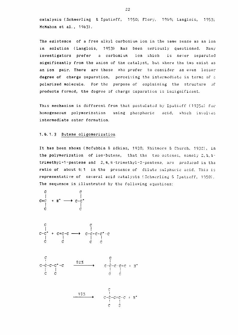
1.b. 1. 3 Butene Oligomerization

1.b. 2 Thermodynamics of Alkene Oligomerization

1. 7 Reactors for Determining the Kinetics of Heterogeneous

Catalytic Reactions

1.7. 1 Background

1.7. 2 Gradientless Reactors

1. 7.2. 1 Recycle Reactors

1. 7. 2. 2 The Internal Recirculation Type

Gradientless Reactor (Internal

Recycle Reactor)

1.7. 2. 3 Examples of the Use of Gradientless

Reac~ors to Obtain Kinetic Data

1.8 Objectives of the Present Study

MICRO-CATALYTIC PULSE REACTOR STUDIES

2. 1 Introduction - Literature Review

2. 1. 1 Background

2. 1. 2 Pulse Reactor Types and Techniques

2. 1. 2. 1 Elution with Reaction

17

17

17

22

27

27

30

32

33

34

34

35

vi

2. 1. 2. 2 Hicrocatalytic Technique

2. 1. 2. 3 Deuterium Exchange

2. 1. 2. 4 Reactor-Stop Technique

2. 1. 2. o Sample Vacancy Technique

2. 1. 2.7 Heater Displacement Technique

2. 1. 3 Analysis of Pulse Reactor Data

2. 1. 3. 1 Reactions of the Type A~ B

2. 1. 3.2 Reversible Reactions of the Type

A~ B + C

2.1.3. 3 Consecutive Reactions

2. 1. 4 Advantages and Disadvantages of the Pulse

Technique

2. 1.5 Applications of the Pulse Technique

2. 2 Objectives of the Pulse Micro-Catalytic Studies

2. 3 Experimental Apparatus and Procedure

2. 3. 1 The Pulse Technique Used in This Study

2. 3. 2 The Reactor System

2. 3. 3 Experimental Procedure and Analysis

2. 3. 3. 1 Reaction Conditions

2. 3. 3. 2 Typical Run Procedure

2. 3. 3. 3 Phosphoric acid Concentrations

2. 3. 3. 4 Product Analyses

35

35

3&

3b

3b

3b

37

37

37

40

41

42

42

42

45

45

4b

47

vii

2. 3. 3. 5 Reaction Data Rorkup

2. 4 Reactor System Characterization

2. 4. 1 Gas Chromatograph Calibration

2.4.2 The Input and Output Pulse

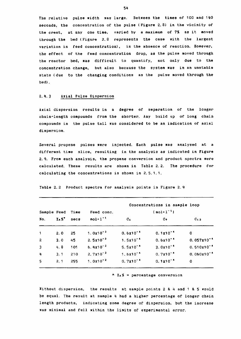
2.4. 3 Axial Pulse Dispersion

2. 4. 4 Single Slice Analysis

2. 4. 5 Hass Balance in Absence of Reaction

2. 4. b Reproducibility

2. 4. 7 Catalyst Activity and Lifetime

2.4. 8 Differential Analysis

2. 4. g Equilibrium Conversions

2.4. g. 1 Equilibrium Compositions of Straight

Alkenes

2. 4. g. 2 Equilibrium Composition of C4, c,, C6,

C1 and Ca Alkene Groups

2. 4. g. 3 Equilibrium Compositions of a Combined

C4, c,, C6 and C1 Alkana Group

2. 4.g. 4 Equilibrium Compositions of a Group of

Alkanes

2. 4. 10 Determination of Phase Equilibria

2.5 Results and Discussion

2. 5. 1 Preliminary Results

2. 5. 1. 1 Complete Analysis of Typical Pulse

Experiment

52

54

So

57

57

58

58

58

bO

b1

b1

b5

bb

b8

08

b8

viii

2. 5. 2 Pure Propene results

2.5. 2.1 Product Spectra

2. 5. 2. 2 Reaction Pathways

2. 5.2. 3 Propene Rate-Concentration Data

2.5. 3 Pure 2-Methyl-1-Pentene

2. 5.3. 1 Product Spectra

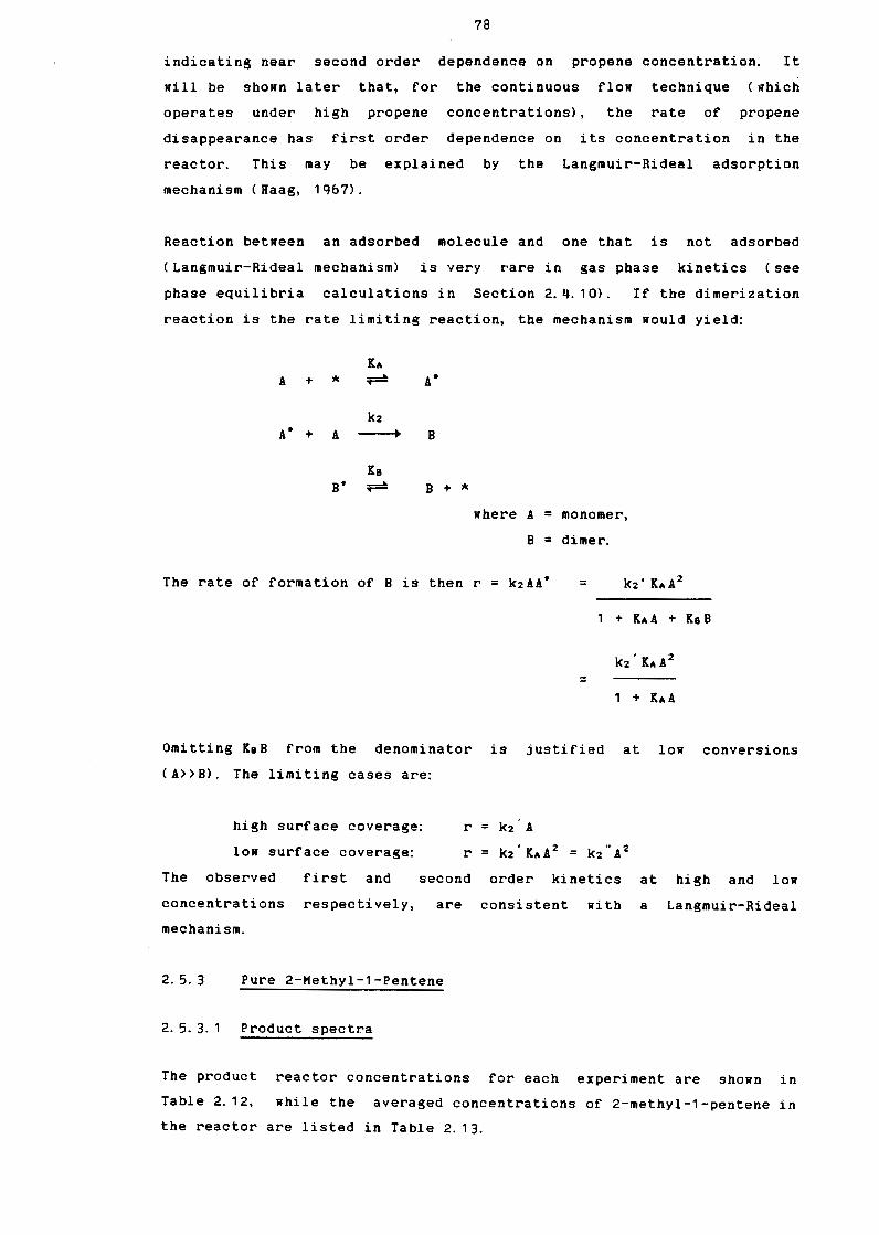
2. 5. 3. 2 Reaction Mechanisms

2.5.3.3 2-Methyl-1-Pentene Rate-Concentration

Data

2.5.4 Results for Various Other Rexene Isomers

2.5. 5 Pure 1-Butene Results

2.5. 5. 1 Product Spectra

2.5.5. 2 Reaction Mechanisms

2. 5. 5. 3 Rate-Concentration Data for 1-Butene

2.5. b Pure Isa-Butene Results

72

72

73

77

78

78

83

83

84

84

85

88

8g

2.5. b. 1 Product Spectra Sg

2. 5.6.2 Reaction Mechanisms 8g

2.5. b. 3 Rate-Concentration Data for Isa-Butene g2

2. 5. 7 Comparison of the Pure Feed Results

2. 5. 8 Propane+ 2-Hethyl-1-Pentene

2. 5. 8. 1 Feed and Product Spectra g3

2. 5.8. 2 Reaction Mechanisms

ix

2.5.q Propene + 2-Hethyl-2-Pentene

2. 5. 10 2-Methyl-1-Pentene + 1-Butene

2. 5. 10. 1 Feed and Product Spectra


2.5. 11 2-Methyl-1-Pentene + Isa-Butene

2.5. 11. 1 Feed and Product Spectra

2.5. 11. 2 Reaction Mechanisms

2.5. 12 Propene + 1-Butene


2. 5. 12.2 Reaction Mechanisms

2.5. 13 Propene + Isa-Butene


2.5. 13.2 Reaction Mechanisms

2.b Conclusions

2. b. 1 Oligomerization of Pure Olefins

2.b.2 Hixed Feeds Oligomerization

3. KINETIC STUDIES USING AN INTERNAL GAS RECIRCULAiION REACTOR

3. 1 Introduction

3. 1. 1 The Use of Gradientless Reactors to Obtain

Intrinsic Kinetic Data

3. 1. 1. 1 Residence Time Distribution Studies

3. 1. 1. 2 Interphase Transport Effects

100

100

101

102

104

104

105

108

108

108

110

111

112

114

114

120

120

120

121

125

X

3. 1. 1. 3 Intraparticular Diffusion Effects

3. 1. 1. 4 Superficial Gas Velocities and the

Recycle Ratio

3. 1. 2 The Modelling of Kinetic Data Obtained from

Gradientless Reactors

127

130

132

3. 1.2. 1 Background to Kinetic Hodels 132

3. 1. 2.2 Building Kinetic Hodels 133

3. 1.2.3 Solving and Analysing Kinetic Hodels 135

3. 1. 2. 4 Tests for Hodel Accuracy 137

3.1. 2.5 Use of Diagnostic Parameters 137

3. 1. 2.6 Empirical Modelling Techniques 138

3. 1. 2.7 Examples of Kinetic Studies and Modelling 138

3. 1. 3 Literature Review of Kinetic Studies on the

Catalytic Polymerization Over Solid Phosphoric

Acid

3. 1. 3. 1 The Effect of Phosphoric Acid

Concentration

3. 1. 3. 2 The Effect of Space Velocity, Pressure

and Olefin Concentrtion

3. 1. 3. 3 The Effect of Temperature

3. 1. 3. 4 The Effect of Feed Composition

3. 1. 3. 5 The Effect of Process Variables on

Product Yield and Quality

3. 1. 3. 6 The Effect of Transport Resistances

3. 2 Objectives of the Kinetic Studies

142

143

143

143

146

147

147

xi

3, 3 Experimental Apparatus and Procedure


3. 3. 1. 1 The Reactor System Used for the Residence

Time Distribution Studies

3. 3. 1.2 The Reactor System Used for the Hass

Transfer Studies (Ko Reaction)

3. 3. 1. 3 The Reactor System Used for the Kinetic

Studies

3. 3.2 The Reactor


3.4 Results


3. 3.3. 2 Hass Transfer Studies

3. 3. 3. 3 Kinetic Studies (and Hass Transfer

with Reaction)

3. 3.3. 4 Product Analyses

3. 3. 3.5 Reaction Data Rorkup

3. 4.1 Reactor Characterization Rithout Reaction


3. 4. 1. 2 Interphase Hass Transfer Studies Using

Napthalene

3. 4. 2 Reactor Characterization with Reaction

3. 4. 2. 1 Detailed Analysis of a Typical Run

3. 4. 2. 2 Hass Balance over the Reactor

148

150

151

153

157

157

157

1 b2

1b2

1b3

1b3

1b3

1 b7

170

170

175

xii

3. 4. 2. 3 Catalytic Activity of the Empty Reactor 17b

3. 4.2. 4 Reproducibility and Steady State

Behaviour of Experiments

3. 4. 2.5 Equilibrium Conversions and Phase

Equilibria

3. 4. 2.b Hass Transfer with Reaction

3.4.3 Preliminary Results

3. 4.4 Propene Oligomerization Experiments

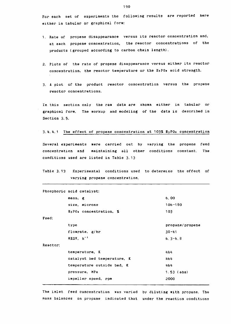
3. 4.4.1 The Effect of Propene Concentration at

17b

181

18b

18g

103% HJP04 Concentration 1go

3. 4. 4. 2 The Effect of Propene Concentration at

114% HJP04 Concentration 1g2

3.4. 4. 3 The Effect of Temperature at 111% H3P04

Concentration

3. 4. 4. 4 The Effect of Temperature at 102% H3P04 1ga

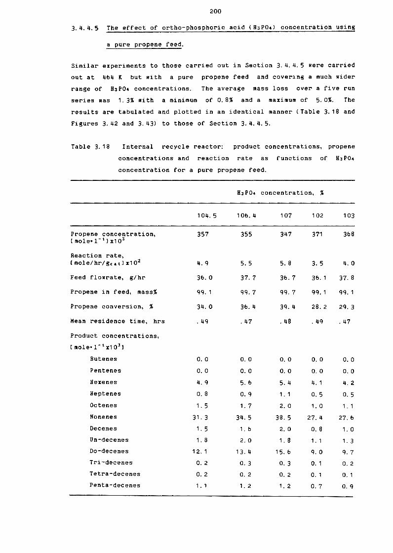
3. 4. 4. 5 The Effect of Ortho-Phosphoric Acid

(H3P04) Concentration Using a Pure Propane

Feed 200

3. 4.4. b Low Conversion Experiments 202

3. 4.5 1-Butene Oligomerization Experiments 202

3. 4.5. 1 The Effect of 1-Butene Concentration 204

3. 4. 5. 2 The Effect of Temperature 205

3. 4. 5. 3 The Effect of Acid Concentration 20g

3. 4. b The Oligomerization of Isa-Butene 211

3. 4. 7 The Oligomerization of 1-Hexene 212

xiii

3.5 Discussion 214

3.5. 1 The Residence Time Distribution Studies 214

3.5.2 Hass Transfer Studies 215

3.5. 2. 1 Hass Transfer Studies Using Napthalene 215

3.5.2. 2 Intra-particular and Interphase Hass

Transfer with Reaction

3.5. 3 General Qualitative Findings

3.5.3. 1 Propane Experiments

3.5.3. 2 1-Butene and Isa-Butene Experiments

3.5. 4 Simple Power Law Modeling of the Rate

Concentration Data

3.5. 4. 1 Modeling of the Propane Data

3. 5.4.2 Modeling of the 1-Butene Data

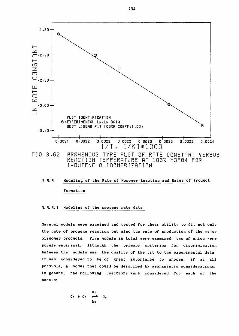
3.5.5 Modeling of the Rate of Monomer Reaction

and Rates of Product Formation

3.5.5.1 Modeling of the Propane Rate Data

3.5.5.2 Modeling of the 1-Butene Rate Data

3.b Conclusions

4. ALKENE OLIGOHERIZATION REACTIONS OBER SOLID PHOSPHORIC ACID,

220

221

221

222

222

222

230

232

232

254

2bb

USING A FIXED BED REACTOR 273

4. 1 Introduction

4. 1. 1 Modelling the Behaviour of Fixed Bed Catalytic

Reactors

4. 2 Objectives of the Fixed Bed Reactor Studies

273

275

27b

xiv

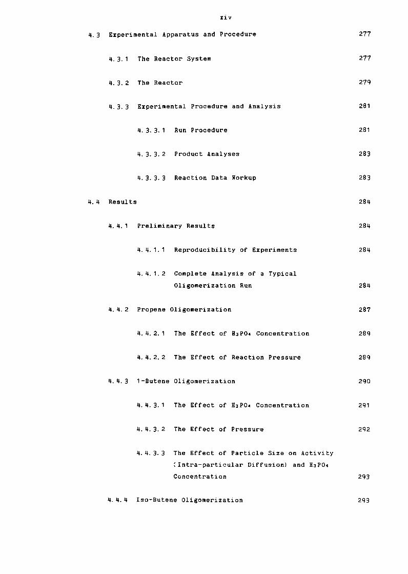
4.3 Experimental Apparatus and Procedure


4. 3. 2 The Reactor


4. 3.3. 1 Run Procedure

4. 3.3.2 Product Analyses

4.3. 3.3 Reaction Data Horkup

4. 4 Results

4.4. 1 Preliminary Results

4. 4. 1. 1 Reproducibility of Experiments

4. 4. 1. 2 Complete Analysis of a Typical

Oligomerization Run

4. 4. 2 Propene Oligomerization

4. 4. 2. 1 The Effect of HJP04 Concentration

4. 4. 2.2 The Effect of Reaction Pressure

4. 4. 3 1-Butene Oligomerization

4.4.3. 1 The Effect of HJP04 Concentration

4.4. 3. 2 The Effect of Pressure

4. 4. 3. 3 The Effect of Particle Size on Activity

:Intra-particular Diffusion) and HJP04

Concentration

4. 4.4 Isa-Butene Oligomerization

277

277

281

281

283

283

284

284

284

284

287

5.

xv

4.5 Discussion

4.5. 1 The Effects of Process Variables

4. 5. 2 Comparison of the Integral Reactor Results with

those of the Internal Gas Recirculation Reactor 2gg

4.5. 3 One Dimensional Analysis of the Integral Reactor 2gg

4.6 Conclusions 302

CONCLUDING REMARKS 305

REFERENCES 311

APPENDICES 328

Appendix A GC Method for Hicrocatalytic Pulse Analysis 32g

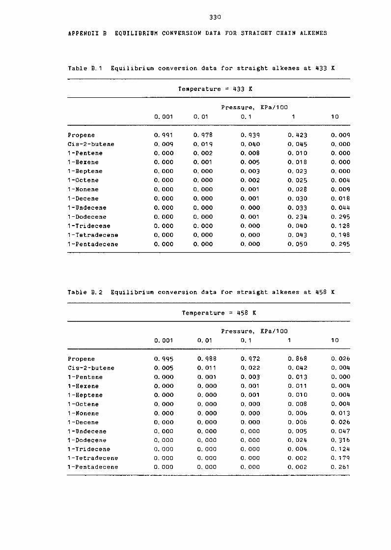
Appendix B Equilibrium Conversion Data for Straight

Chain Alkenes 330

Appendix C Equilibrium Conversion of c, and C6 Alkenes 332

Appendix D Vapour Liquid Equilibria Determination 333

Appendix E GC Chromatogram of Typical Propene Oligomer

Product

Appendix F Hass Spectrometer trace of Typical Oliomer

336

Product 337

Appendix G Determination of Compressibility Factor, Z 338

Appendix H Product Spectra and Rate/Concentration data

for Various Alkene Isomers 340

Appendix I GC Method for Gas Analysis 346

Appendix J One Dimensional Analysis of Fixed Bed Reactor 348

Appendix K Description of Procedures Followed By Hass

Balance Program 352

xvi

Appendix L Optimised Solution of Kinetic Hodel' A' of

Section 3. 4. 5. 1 360

Appendix H Experimental and Predicted Rates and Concen

tration Data for each of the Models of Section

3. 5. 5 364

xvii

LIST OF FIGURES

Figure 1. 1

Figure 1. 2

Figure 1. 3

Figure 1.4

Figure 1.5

Figure 1. b

Figure 1.7

Figure 2. 1

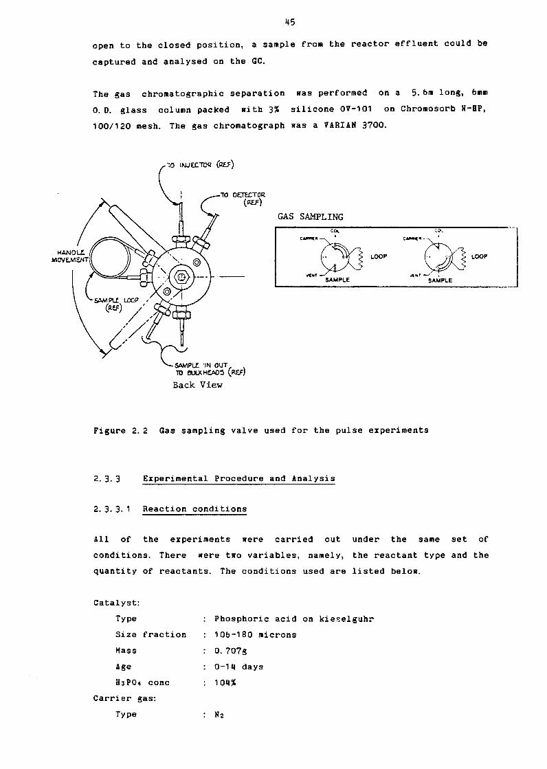
Figure 2.2

Figure 2.3

Figure 2. 4

Figure 2. 5

Figure 2. b

Figure 2. 7

Figure 2. 8

Flow Diagram of the SASOL Plants at Secunda

Approximate Molecular Composition of Strong

Phosphoric Acids in terms of the Number, n,

of Phosphorus Atoms in the Molecule-ion.

Free Energy Change during Dimerization

Equilibrium Conversion for Propane Dimerization

to 1-Hexene and trans-3-Hethyl-2-Pentene

Free Energy Changes for the Polymerization of

Propene

Standard Berty type Internal Recycle Reactor

( Fixed Basket)

Schematic of Pulse Reactor System

Gas Sampling Valve used for the Pulse Experiments

HJP04 Concentration as a Function of Rater Vapour

Pressure over the range g7% to 104% H3P04

H3P04 Concentration as a Function of Rater Vapour

Pressure over the range 100% to 108% H3P04

Pulse: GC Calibration: Propene & Butanes

Pulse: GC Calibration: Hexenes

The Input & Output Pulses using a 2-Methyl-1-

Pentene Feed

Output Pulse and Bed Residence Time using a

2-Hethyl-1-Pentene Feed

PAGE

3

11

12

24

25

2b

31

43

45

48

48

50

50

53

53

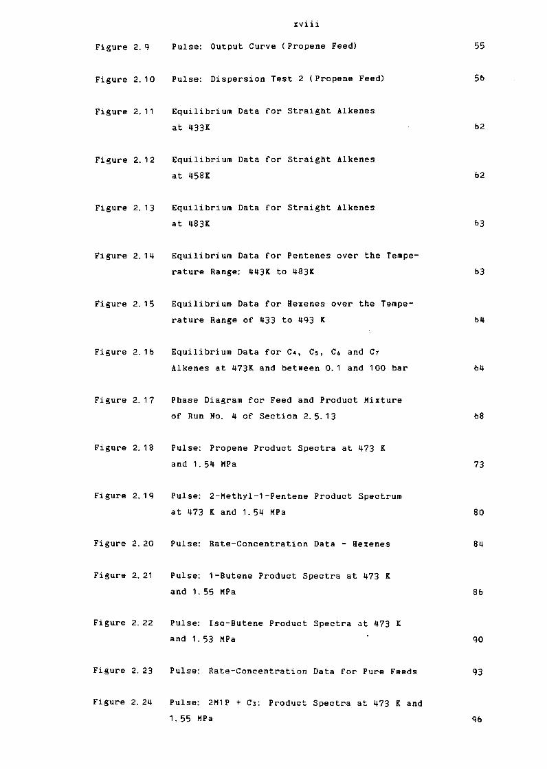
Figure 2.g

Figure 2. 10

Figure 2. 11

Figure 2. 12

Figure 2. 13

Figure 2.14

Figure 2. 15

Figure 2. 1b

Figure 2. 17

Figure 2. 18

Figure 2. 1q

Figure 2. 20

Figure 2. 21

Figure 2.22

Figure 2. 23

Figure 2. 24

xviii

Pulse: Output Curve (Propene Feed)

Pulse: Dispersion Test 2 (Propene Feed)

Equilibrium Data for Straight Alkenes

at 433K


at 458K


at 483K

Equilibrium Data for Pentenes over the Tempe

rature Range: 443K to 483K

Equilibrium Data for Hexenes over the Tempe

rature Range of 433 to 4q3 K

Equilibrium Data for C4, c,, Cb and C1

Alkenes at 473K and between 0. 1 and 100 bar

Phase Diagram for Feed and Product Mixture

of Run No. 4 of Section 2.5. 13

Pulse: Propane Product Spectra at 473 K

and 1. 54 HPa

Pulse: 2-Hethyl-1-Pentene Product Spectrum

at 473 Kand 1.54 HPa

Pulse: Rate-Concentration Data - Hexenes

Pulse: 1-Butene Product Spectra at 473 K

and 1. 55 HPa

Pulse: !so-Butene Product Spectra at 473 K

and 1. 53 HPa

Pulse; Rate-Concentration Data for Pure Feeds

Pulse: 2H1 P + CJ: Product Spectra at 473 K and

1.55 11Pa

55

5b

b2

b2

b3

63

64

b4

68

73

80

84

8b

go

Figure 2.25

Figure 2. 2b

Figure 2. 27

Figure 2.28

Figure 2.29

Figure 3. 1

Figure 3.2

Figure 3. 3

Figure 3:4

Figure 3. 5

Figure 3. b

Figure 3. 7

Figure 3. 8

xix

Pulse: Ct2 (Product) vs 2H1P Concentration

Taken from the Data of Table 2. 12.

Pulse: 2H1P + 1-Butene: Product Spectra

at 473 Kand 1. 53 HPa

Pulse: I so-Butene + 2M1 P: Product Spectra

at 473 Kand 1. 54 MPa

Pulse: 1-Butene + Propene: Product Spectra

at 473 Kand 1.53 MPa

Pulse: I so-Butene + Propene: Product Spectra

at 473 Kand 1. 55 HPa

Schematic Diagram of the Tanks-in-Series Hodel

The Effectiveness Factor as a Function of

the Parameter ML for Various Catalyst Shapes

and for Volume Change during Reaction

Different Rate Controlling Regimes for Strongly

Exothermic Reactions in Porous Catalysts

Different Rate Controlling Regimes for Strongly

Exothermic Reactions in Porous Catalysts

FloR Device for Measuring Pressure Drop Versus

FloRrate through the Bed in an Internal Recycle

Reactor

Comparison of the Rate Constants of both

Langlois & Ralkey and Bethea & Karchmer at

Equivalent Acid Concentrations

Bethea & Kacctmer' s Rate Constant as a Function

of the Ortho-Phosphoric Acid Concentration

Arrhenius Plots of both Bethea & Karchmer and

Langlois & Ralkey

gg

102

105

1 og

112

123

128

1 31

1 41

142

144

Figure 3,q

Figure 3.10

Figure 3. 11

Figure 3. 12

Figure 3. 13

Figure 3. 14

Figure 3.15

Figure 3. 1b

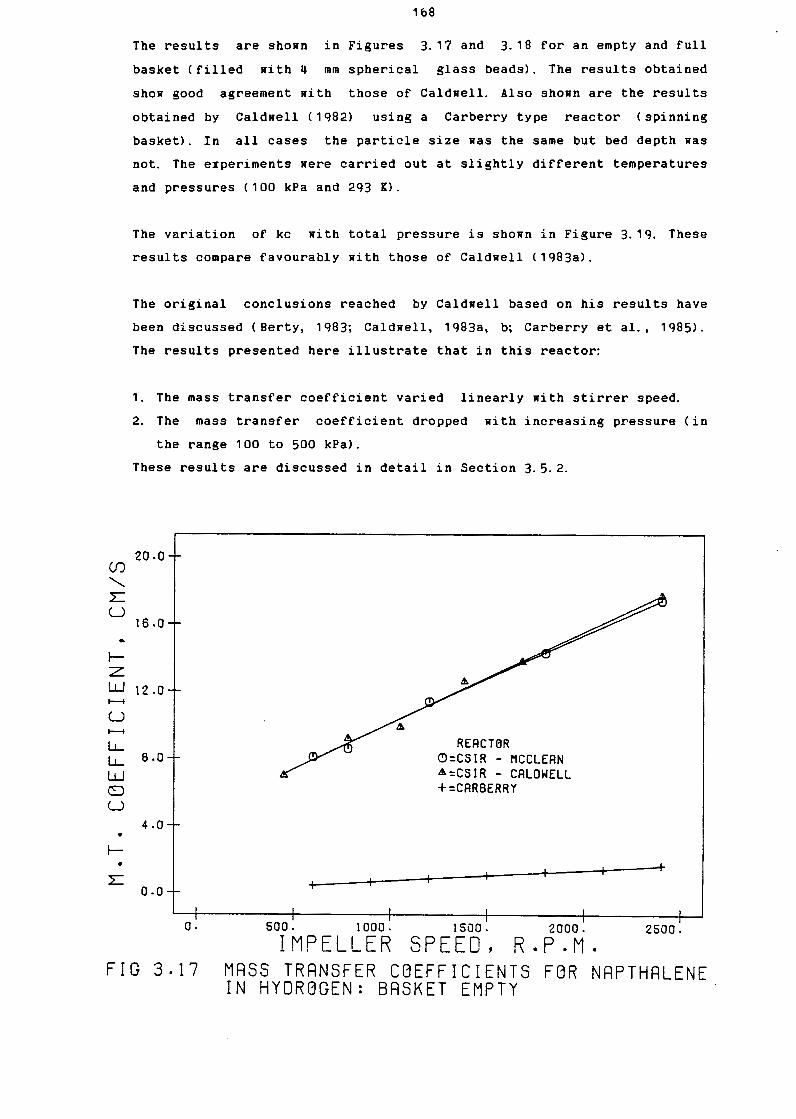
Figure 3. 17

Figure 3. 18

Figure 3. 1g

Figure 3. 20

Figure 3. 21

Figure 3. 22

Figure 3. 23

xx

Rate Constant Correction Factor of HcHahon et al.

A Comparison of the Observed and Predicted

Rate Constants produced by HcHahon et al.

Reactor System used for Residence Time

Studies

The Reactor system used for the Hass Transfer

Studies

Schematic of Internal Gas Recirculation Reactor

System

The Internal Recycle Reactor Assembly

Detailed Diagram of Hagnedrive Assembly

Calculation of Hass Transfer Coefficients

Hass Transfer Coefficients for Napthalene

in Hydrogen: Basket Empty

Hass Transfer Coefficients for Napthalene

in Hydrogen: Basket Full

Hass Transfer Coefficient as a Function of

Pressure: Non-diffusing Component - Air

Typical Oligomerization Experiment

Conversion and RHSV versus Time


Reactor Temperature and Conversion as

functions of time


Liquid Product Concentration and Propene

Conversion versus Time


Rate of Propene Reaction and Conversion

versus Time

145

14b

150

152

154

155

1 b8

172

172

'j 73

174

Figure 3.24

Figure 3. 25

Figure 3. 2b

Figure 3.27

Figure 3.28

Figure 3.2g

Figure 3. 30

Figure 3. 31

Figure 3. 32

Figure 3. 33

Figure 3.34

Figure 3. 35

Figure 3. 3b

Figure 3. 37

Figure 3. 38

xxi


Rater Dew Point in Feed versus Time on Stream

Steady State Behaviour of the Internal Recycle

Reactor: The Effect of Controlling Acid

Concentration

Internal Recycle Reactor Induction Period

Internal Recycle Reactor: Reproducibility

Internal Recycle Reactor: Reaction Rate versus

Impeller Speed at 101.5% HJP04 and 4b4 K

Internal Recycle Reactor: Reaction rate versus

Impeller Speed at 114% HJP04 and 478 K


Particle Size at 4b4 K


Particle Size at 114% H3PQ4 and 503 K

The Effect of Hydration on Reaction Rates

The Effect of Hydration on Product Spectra

Rate of Propane Reaction as a Function of

Propene Reactor Concentration at 103% HJP04

Product Concentrations as Functions of the

Propane Reactor Concentration at 103% HJP04

Rate of Propene Reaction as a Function of the

Propane Reactor Concentration at 114% H3P04


Propene Reactor Concentration at 1i4% HJP04

Rate of Propane Reaction as a Function of

Temperature at 111% H3PQ4

175

177

180

180

183

183

184

184

188

188

Figure 3. 3g

Figure 3. 40

Figure 3. 41

Figure 3. 42

Figure 3.43

Figure 3. 44

Figure 3. 45

Figure 3. 46

Figure 3. 47

Figure 3. 48

Figure 3_4g

Figure 3.50

Figure 3. 51

Figure 3. 52

xxii

Product Concentrations as functions of the

Reactor Temperature at 111% HJP04

Rate of Propene Reaction as a Function of

Temperature at 102% H3P04

Propene Product Concentrations as Functions

of Reactor Temperature at 102% HJP04

Rate of Propene Reaction as a Function of

B3P04 Concentration for a Pure Propene Feed

Propene Product Concentrations as Functions of

H3PQ4 Concentration for a Pure Propene Feed

The Effect of Conversion on Product

Distribution for a Pure Propene Feed

Rate of 1-Butene Reaction as a Function of the

1-Butene Reactor Concentration


1-Butene Reactor Concentration

Rate of 1-Butene Reaction as a Function of

Temperature at 103% HJP04


Reactor Temperature

Rate of 1-Butene Reaction as J Function of

B3PQ4 Concentration at 446.5 K


H3PQ4 Concentration

Typical Product Spectra from !so-Butene

Oligomerization Over Solid Phosphoric Acid

Typical Product Spectra from 1-Hexene Oligom

erization Over Solid Phosphoric Acid

201

201

203

206

206

208

208

210

210

212

213

Figure 3.53

Figure 3. 54

Figure 3.55

Figure 3.5b

Figure 3.57

Figure 3.58

Figure 3.5g

Figure 3. bO

Figure 3. b1

Figure 3. b2

Figure 3. b3

Figure 3. b4

xxiii

Simple Power Law Fit to Propene Rate/Concentration

Data Obtained at 4b4 Kand 103% HJP04

Power Law Fit to Rate Constant vs H3PQ4 concentra

tion Data at 4b4 K for Propene Oligomerization

Arrhenius Type Plot of Rate Constant as a

Function of Temperature for Propene Oligomerization

223

225

at 102% H3PQ4 225

Predicted and Experimental Propene Reaction Rates

as Functions of Propene Concentration at 4b4 Kand

114% HJP04 227

Percentage Error Analysis as Determined from


as Functions of Propane Concentration at 4b4 Kand

114% H3P04 227


as Functions of Reactor Temperature at 111% HJP04 228

Percentage Error Analysis as Determined from


as Functions of Reactor Temperature at 111% HJP04 22g

Simple Power Law Fit to 1-Butene Rate/Concentra

tion Data at 4b4 Kand 103% HJP04

Power Law Fit to Rate Constant vs HJP04 Concentr

ation for 1-Butene Oligomerization at 44b.5 K

Arrhenius Type Plot of Rate Constant versus

Reaction Temperature at 103% H3PQ4 for 1-Butene

Oligomerization

Hodel P1: Predicted and Experimental Product

Concentrations as Functions of Propene Concentr

ations at 103% HJP04 and 464 K

Hodel P1: Predicted and Experimental Reaction Rates

as Functions of Propene Concentrations at 103%

H3PQ4 and 464 K

231

231

232

235

235

Figure 3.b5

Figure 3. bb

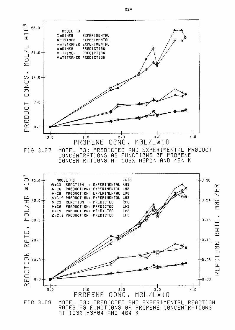
Figure 3. b7

Figure 3. b8

Figure 3.bq

Figure 3. 70

Figure 3.71

Figure 3. 72

Figure 3. 73

xxiv


Concentrations as Functions of Pr~pene Concentr-

ations at 103% HJP04 and 4b4 k 238

Hodel P2: Predicted and Experimental Reaction

Rates as Functions of Propene Concentrations at

103% HJP04 and 4b4 K


Concentrations as Functions of Propene Concentr-

ations at 103% HJP04 and 4b4 K 23q


Rates as Functions of Propene Concentrations

at 103% HJP04 and 4b4 K


Concentrations as Functions of Propene Concen

trations at 103% HJP04 and 4b4 K


Rates as Functions of Propene Concentrations at

103% HJP04 and 4b4 K

Percentage Error Analysis, as determined from the

Predicted and Experimental Dimer Concentration, as

functions of Propene Concentration at 4b4 Kand

241

241

103% HJ P04 for Hodels P1, P2, P3 and P4 242


Predicted and Experimental Trimer Concentration, as

Functions of Propene Concentration at 4b4 Kand 103%

HJP04 for Hodels P1, P2, P3 and P4


Predicted and Experimental Tetramer Concentration,

as functions of Propane Concentration at 4b4 Kand

243

103% HJ PQ4 for Hodels P1, P2, P3 and P4 243

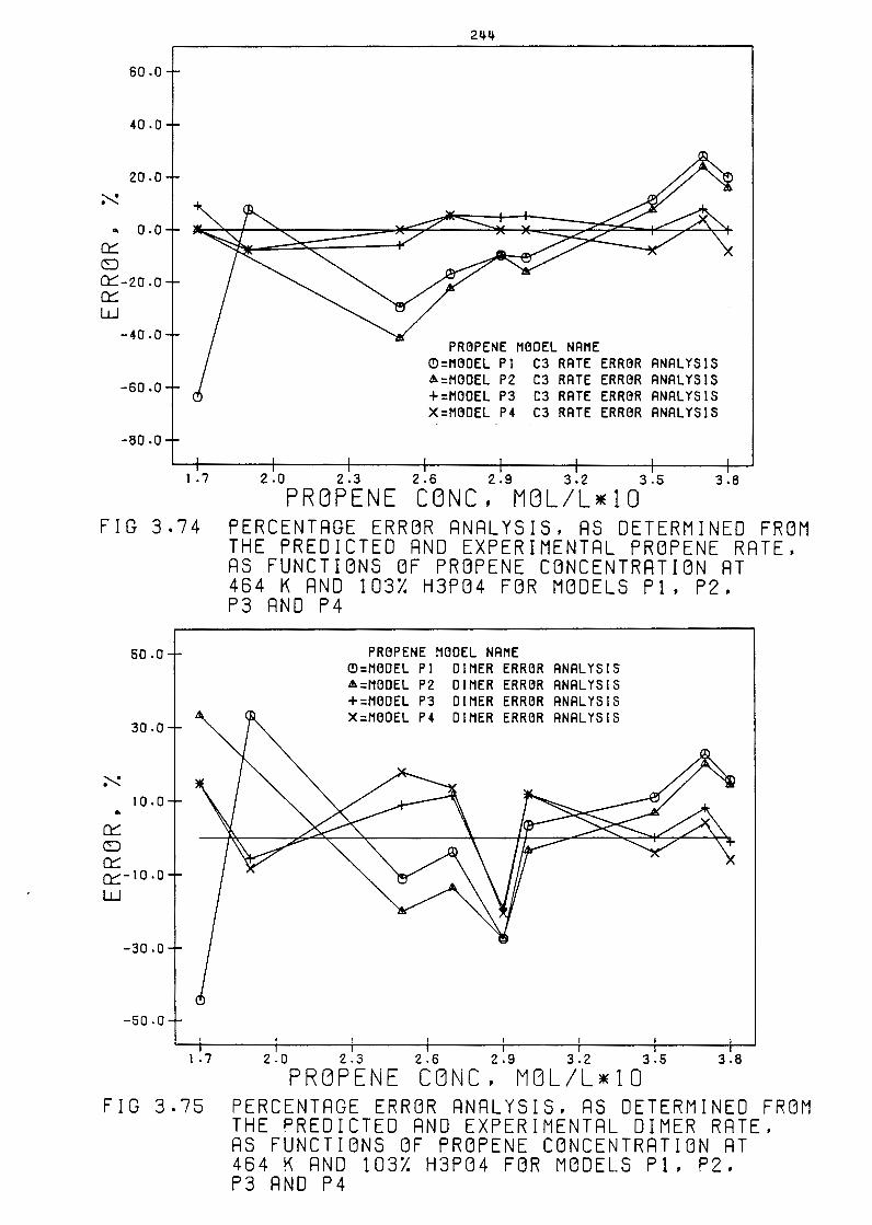
Figure 3.74

Figure 3.75

Figure 3.7b

Figure 3.77

Figure 3. 78

Figure 3.7g

Figure 3. 80

Figure 3. 81

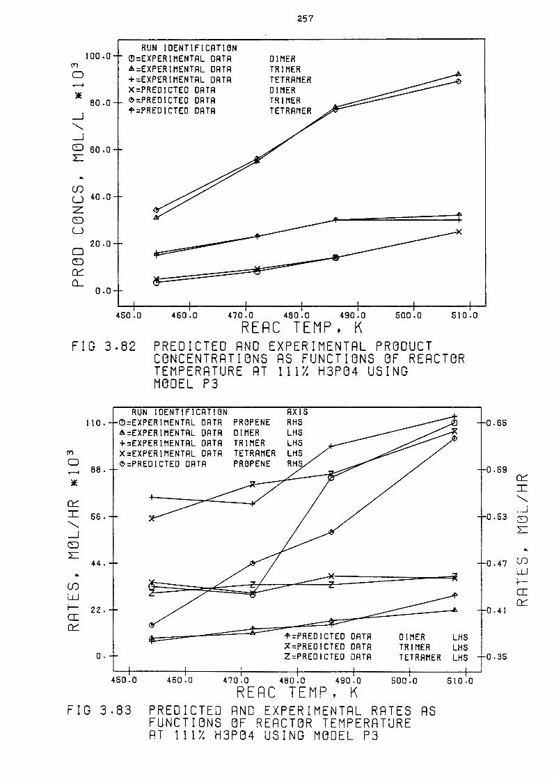
Figure 3. 82

Figure 3. 83

XXV


Predicted and Experimental Propene Rate, as functions

of Propene Concentration at 4b4 Kand 103% H3PQ4 for

Models P1, P2, P3 and P4


Predicted and Experimental Dimer Rate, as functions

of Propene Concentration at 4b4 Kand 103% H3PQ4

for Models P1, P2, P3 and P4

Percentage Error Analysis, as determined from

the Predicted and Experimental Trimer Rate, as


103% H3P04 for Models P1, P2, P3 and P4


Predicted and Experimental Tetramer Rate, as


103% H3 PQ4 for Models P1, P2, P3 and P4

Predicted and Experimental Product Concentrations

as functions of Propene Concentration at 4b4 K

and 114% H3PQ4 using Hodel P3

Predicted and Experimental Rates as functions

of Propane Concentration at 4b4 Kand 114% H3PQ4

using Hodel P3


as functions of Propene Concentration at 464 K

and 114% H3PQ4 using Hodel P4

Predicted and Experimental Rates as Functions of

Propene ~oncentration at 4b4 Kand 114% HJP04

using Hodel P4


as Functions of Reactor Temperature at 111% H3PQ4

244

244

245

245

255

255

256

25b

using Hodel P3 257

Predicted and Experimental Rates as functions of

Reactor Temperature at 111% H3PQ4 using Hodel P3 257

Figure 3.84

Figure 3. 85

Figure 3. Sb

Figure 3. 87

Figure 3.88

Figure 4. 1

Figure 4.2

Figure 4. 3

Figure 4. 4

Figure 4. 5

Figure 4. b

Figure 4. 7

Figure 4. 8

xxvi


as functions of Reactor Temperature at 111% H3PQ4

using Hodel P4

Predicted and Experimental Rates as functions of

258

Reactor Temperature at 111% H3PQ4 using Hodel P4 258

Hodel 84: Predicted and Experimental Product

Concentrations as Functions of 1-Butene Concentr

ation at 103% HJP04 and 464 K

Hodel 84: Predicted and Experimental Reaction Rates

as Functions of 1-Butene Concentrations at 103%

HJP04 and 464 K

I Percentage Error Analysis, as determined from the

Predicted and Experimental Concentration at 464 K

and 103% H3PQ4 for Hodel 84

Schematic of Fixed Bed Reactor System

Micro-reactor Developed by Snel

Schematic Layout of the Packed Small Reactor Volume

Integral Reactor Reproducibility Runs: 1-Butene

Conversion as a Function of Time on Stream

Integral Reactor Reproducibility Runs: Catalyst

Bed Temperature During the Run as a Function of

Catalyst Bed Depth

1-Butene Conversionn and RHSV as Functions of

Time on Stream

Product Spectra as a Function of Time on Stream

for a Typical Oligomerization Experiment using

a 1-Butene feed

Integral Reactor: Propene Oligomerization

Product Spectrum Versus Time on Stream for

Different Acid Concentrations

263

263

264

278

280

282

285

285

287

288

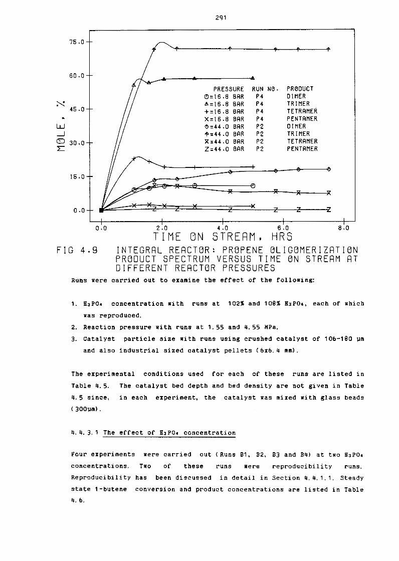
Figure 4.g

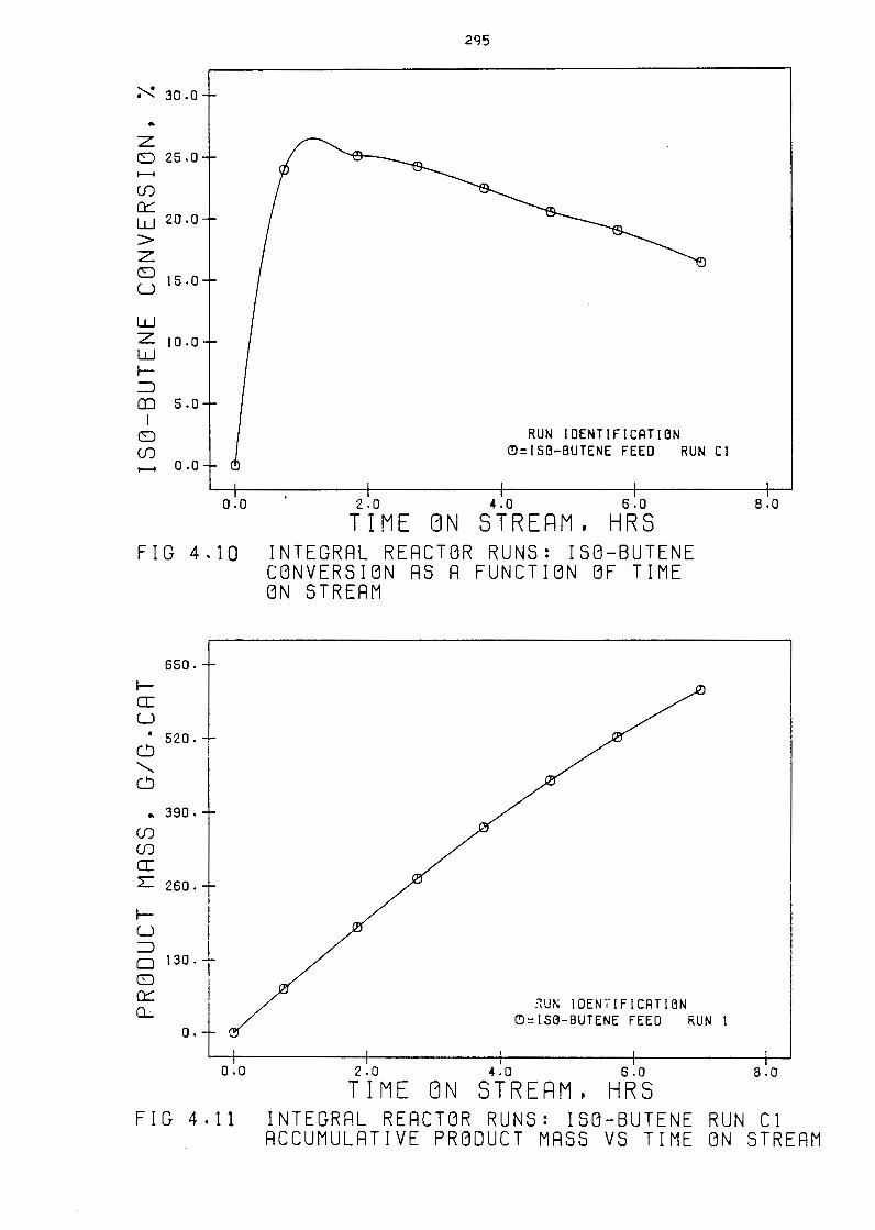
Figure 4. 10

Figure 4. 11

Figure 4. 12

Figure E. 1

Figure F. 1

xxvii

Integral reactor: Propene Oligomerization

Product Spectrum Versus Time on Stream at

Different Reactor Pressures

Integral reactor Runs: Isa-Butene Conversion as

a Function of Time on Stream

Integral Reactor Runs: Isa-Butene Run C1

Accumulative Product Hass Versus Time on Stream

Integral Reactor Runs: Isa-Butene Run Nos. C1-C4

Hole Fractions of Dimer, Trimer and Tetramer

GC Chromatogram of Typical Propane Oligomer Product

Hass Spectrometer Trace of Typical Oligomer Product

2%

336

337

xxviii

LIST OF TABLES

Table 1. 1

Table 1.2

Table 1. 3

Table 1. 4

Table 1. 5

Table 2. 1

Table 2.2

Table 2. 3

Table 2. 4

Table 2. 5

Table 2. b

Table 2. 7

Table 2. 8

Table 2. g

Table 2. 10

Table 2. 11

Product Selectivities of the SASOL Fixed Bed and

Synthol Reactors

Selected Properties of Liquid and Solid Products

from SASOL Reactors

The Relationship between the Cationic and Anionic

Oxides in Phosphates

Standard Free Energy Change (kcal) of Polymeriza

tion per Monomer Unit Added

Summary of Laboratory Reactor Ratings

Relative Response Factors of Hydrocarbons

Product Spectra for analysis Points in Figure 2.g

Product Spectra for Analysis Points in Figure 2. 10

Concentrations for Propane Reproducibility Tests

Alkanes Used in the Equilibrium Calculation of

Section 2. 4.g. 4

Area Counts and Concentrations for a Typical

Pulse

Concentrations in the Reactor Exit

Product Spectra for Pure Propane at 473 Kand

1. 54 HPa

Averaged Reactor Concentrations of the Feed

Pure Oligomer Fractions Prior to Cracking

Rate Concentration Data for Pure propane

PAGE

3

g

2b

28

51

54

55

57

b5

71

72

73

77

77

Table 2. 12

Table 2. 13

Table 2. 14

Table 2. 15

Table 2. 1b

Table 2. 17

Table 2. 18

Table 2. 1g

Table 2. 20

Table 2. 21

Table 2. 22

Table 2. 23

Table 2. 24

Table 2. 25

Table 2. 2b

Table 2. 27

Table 2. 28

xxix

Product Spectra for 2-Hethyl-1-Pentene at 473 K

and 1.54 HPa

Averaged 2-Hethyl-1-Pentene Concentration

Estimated Molar Ratios of C12 to Cracked Products

in Table 2.8 Based on the Results of Both Tables 2. 8

and 2. 12

Rate Concentration Data for 2-Hethyl-1-Pentene

Reaction Orders for C6 Isomer Polymerization

Product Spectra for 1-Butene at 473 Kand 1.55 HPa

Average Reactor Concentrations of the Feed

Rate-Concentration Data for 1-Butene

Product Spectra for Isa-Butene at 473 Kand 1. 53

HPa

Averaged Reactor Concentrations of the Feed

Rate-Concentration Data for Isa-Butene

Reactant Feed Concentrations at the Reactor

Inlet at 473 Kand 1.55 HPa

Product Spectra at Reactor Exit

Reactant's Reactor Concentrations and Conversion

Levels

Fraction of Ct2 Produced from C6 + C6 and c, + CJ

Reactor Concentrations at the Reactor Inlet at 473 K

and 1. 53 MPa

Product Spectra at the Reactor Exit

81

83

84

85

85

9g

go

100

1 Qi

1 01

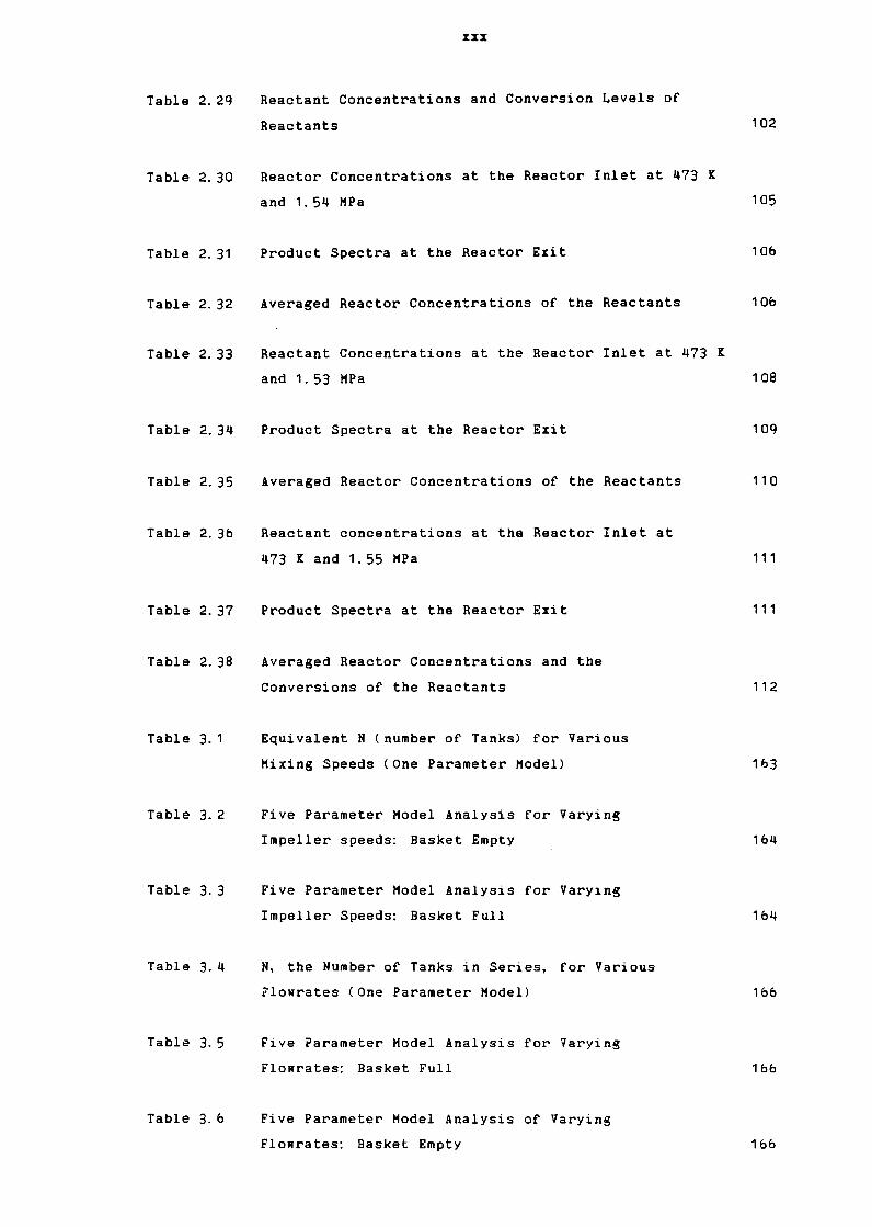
Table 2. 2g

Table 2.30

Table 2. 31

Table 2.32

Table 2. 33

Table 2.34

Table 2. 35

Table 2. 3b

Table 2.37

Table 2.38

Table 3. 1

Table 3. 2

Table 3. 3

Table 3. 4

Table 3. 5

Table 3.6

XXX

Reactant Concentrations and Conversion Levels of

Reactants

Reactor Concentrations at the Reactor Inlet at 473 K

and 1. 54 HPa


Averaged Reactor Concentrations of the Reactants

Reactant Concentrations at the Reactor Inlet at 473 K

and 1.53 HPa


Averaged Reactor Concentrations of the Reactants

Reactant concentrations at the Reactor Inlet at

473 Kand 1.55 HPa


Averaged Reactor Concentrations and the

Conversions of the Reactants

Equivalent N (number of Tanks) for Various

Mixing Speeds (One Parameter Hodel)

Five Parameter Hodel Analysis for Varying

Impeller speeds: Basket Empty


Impeller Speeds: Basket Full

N, the Number of Tanks in Series, for Various

rlowrates (One Parameter Hodel)


Flowrates: Basket Full

Five Parameter Hodel Analysis of Varying

Flowrates: Basket Empty

102

105

1 Ob

1 Ob

108

1 og

110

111

111

11 2

H>3

164

164

166

166

1b6

Table 3.7

Table 3.8

Table 3.q

Table 3. 10

Table 3.11

Table 3. 12

Table 3. 13

Table 3. 14

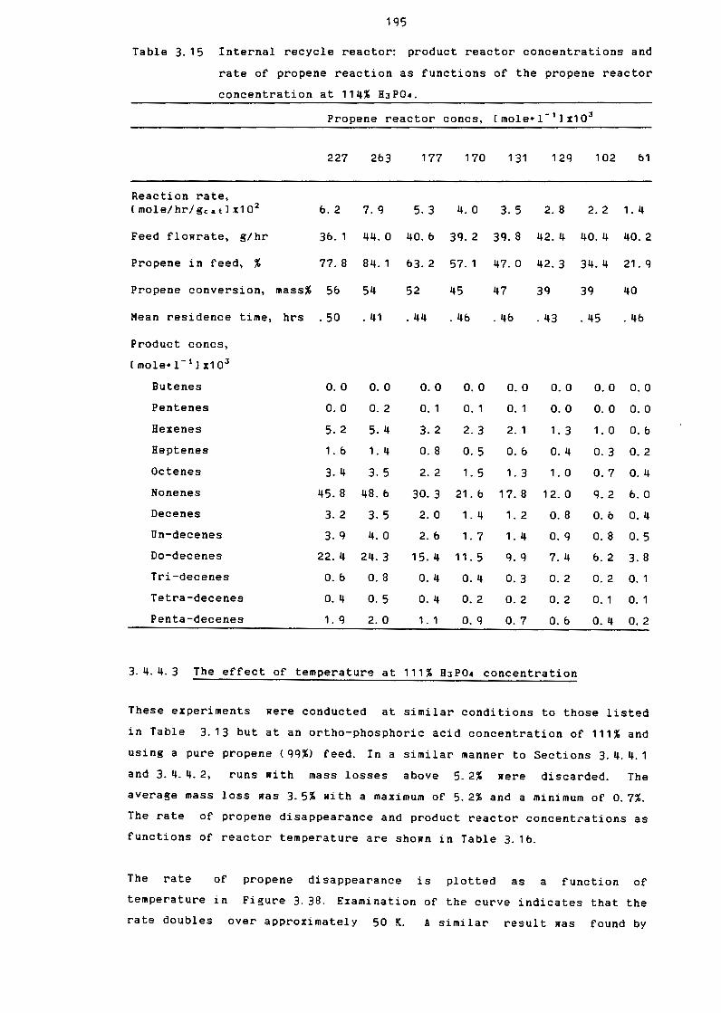
Table 3. 15

Table 3. 1b

Table 3. 17

xxxi

N, Number of Tanks in Series, for Various

Temperatures: Basket Empty

Experimental Conditions for Typical Oligomerization

Run of Section 3. 4. 2.1

Rater Balance Over the Internal Recirculation

Reactor

Experimental Conditions for Bulk Gas Phase Hass

Transfer Experiments

Experimental Conditions used for Intra-particular

Diffusion Experiments

Experimental Conditions Used to Examine the Effect

of Catalyst Hydration on Reactor Behaviour

Experimental Conditions Used to Determine the

Effect of Varying Propane Concentration

Internal Recycle Reactor: Product Reactor

Concentrations and Rate of Propane Reaction as

Functions of Propane reactor Concentrations

at 103% H3PQ4


Concentrations and Rate of Propane Reaction as

Functions of the Propane Reactor Concentration

at 114% HJP04


Concentrations and Rate of Propene Reaction as

Functions of Reaction Temperature at 111% HJP04


Concentration and Rate of Propene Disappearance

as Functions of Reactor Temperature at 102%

HJ PQ4

167

171

178

182

185

187

1 g5

1%

1 gs

Table 3. 18

Table 3. 1g

Table 3. 20

Table 3. 21

Table 3. 22

Table 3. 23

Table 3. 24

Table 3. 25

Table 3. 2b

Table 3. 27

Table 3. 28

Table 3. 2g

xxxii

Internal Recycle Reactor: Product Concentrations,

Propene Concentrations and Reaction Rate as

Functions of H3P04 Concentration for a pure

Propene Feed

Product Spectra, Reaction Rate and Propene

Concentration as Functions of Propene Conversion

Conditions Used for the Oligomerization of

1 -Butene


Concentrations and Rate of 1-Butene Reaction as

Functions of 1-Butene Concentrations


Concentrations, 1-Butene Reactor Concentrations

and Reaction Rates as Functions of Reactor

Temperature

Internal Recycle Reactor: Product Concentrations,

Reaction Rates and 1-Butene Concentrations as

Functions of H3PQ4 Concentration

Internal Recycle Reactor: Isa-Butene Product

Spectra

Internal recycle Reactor: 1-Hexene Product Spectra

and Reaction Rate

Conditions used to Obtain Superficial Gas

Velocities for the Napthalene-air System

Superficial Velocities Estimated from Various

Pressure Drop Equations

Superficial Gas Velocities Estimated from Hass

iransfer Coefficients

Predicted and Experimental Rates of Propene

Reaction at 4f:>4 Kand 114% H3PQ4

200

202

204

205

207

20g

212

213

217

226

Table 3. 30

Table 3. 31

Table 3.32

Table 3. 33

Table 3. 34

Table 3. 35

Table 3. 3b

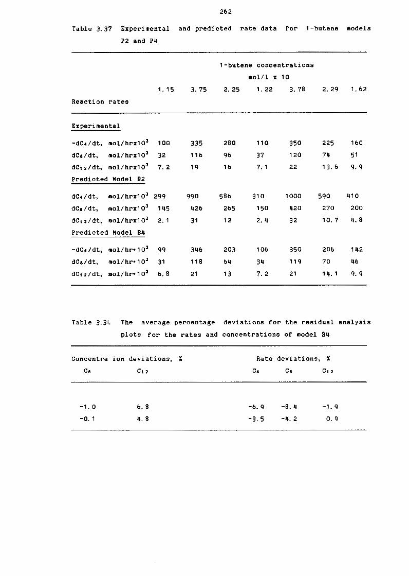
Table 3. 37

Table 3. 38

Table 3. 3q

Table 3. 40

xxxiii

Predicted and Experimental Rates of Propene

Reaction at 111% HJP04

The Average Percentage Deviation Lines for the error

Analysis Plots of Both the Oligomer Concentrations

and Rates of Reaction/Production for the Hodels

P1 to P4

The Calculated Rate Constants kt, kJ, k, and kq

of Hodel P3 at Various Temperatures Calculated from

the Data of Table 3. 17 24g


of Hodel P3 at Various H3PQ4 Concentrations

Calculated from the Data of Table 3.18


of Hodel P4 at Various Temperatures Calculated

from the Data of Table 3. 17

The Calculated Rate Constants kt, kJ, k1 and kq

of Hodel P3 at Various H3PQ4 Concentrations

Calculated from the Data of Table 3. 18

Experimental and Predicted Concentration Data for

1-Butene Hodels 82 and 84

Experimental and Predicted Rate Data for 1-Butene

Hodels P2 and P4

The Average Percentage Deviations for the Residual

Analysis Plots for the Rates and Concentrations of

250

251

252

261

2b2

Hodel B4 2b2

The Calculated Rate Constants kt, kJ and k5 of

Hodel B4 as Calculated at the Conditions of the

Experiments in Table 3. 22

The Rate Constants kt, kJ, and k, of Hodel B4

at Various HJP04 Concentrations calculated from

the Data of Table 3. 23

2b5

2b5

Table 4. 1

Table 4. 2

Table 4.3

Table 4. 4

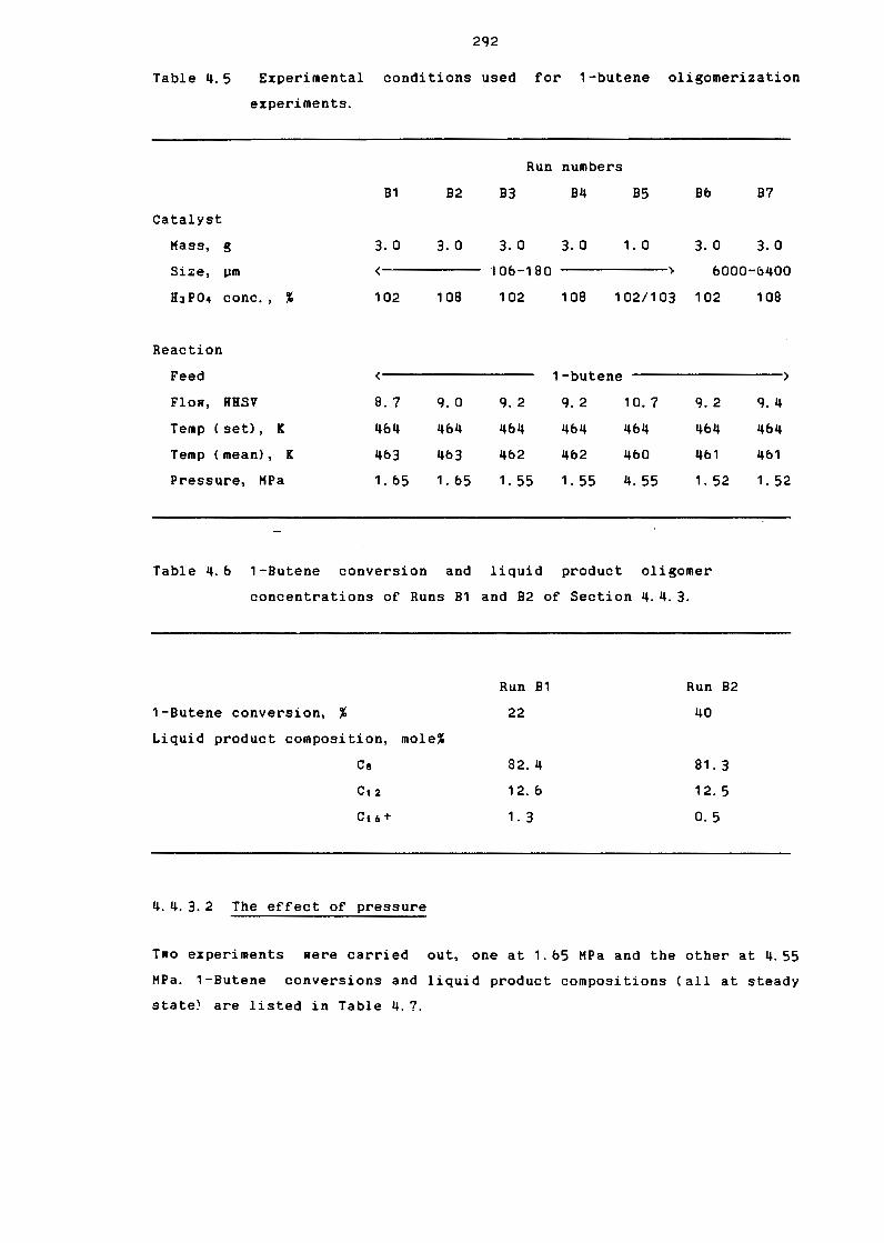
Table 4.5

Table 4.b

Table 4. 7

Table 4. 8

Table 4.g

Table 4. 10

Table B. 1

Table B. 2

Table B. 3

Table C. 1

xxxiv

Experimental Conditi0ns for Typical Oligomerization

Run uf Section 4. 4. 1. 2

Experimental Conditions Used for Propene

Oligomerization Experiments

Propene Conversion and Liquid Product Oligomer

Concentrations of Runs 1,3 and 4 of Section 4.4. 2

Propene Conversion and Liquid Product Oligomer

Compositions of Runs P1, P2 and P4 of Section 4. 4. 2

Experimental Conditions Used for 1-8utene


1-8utene Conversion and Liquid Product Oligomer

Concentrations of Runs 81 and 82 of Section 4. 4. 3

1-8utene Conversion and Liquid Product Oligomer

Concentrations of Runs 81 and 85 of Section 4.4. 3

1-Butene Conversion and Liquid Oligomer

28b

288

Concentrations of Runs Bb and 87 of Section 4. 4. 3 2q3

Experimental Conditions Used for Isa-Butene


Results of the One Dimensional Hodel Analysis

for Propene Oligomerization at the Conditions

Described for Run 1 in Table 4. 2

Equilibrium Conversion Data for Straight Alkenes

at 433 IC

£quilibrium Conversion Data for Straight Alkenes

at 458 IC

Equilibrium Conversion Data for Straight Alkenes

at 483 IC

Equilibrium Conversion of a Group of C5 Alkenes

301

330

330

331

332

Table C. 2

Table G. 1

XXXV

Equilibrium Conversion of a Group of C6 Alkenes

Second Virial Coefficients and Compressibility

Factor for Propene-Nitrogen Mixture

332

Table H. 1 Product Spectra for 2-Hethyl-2-Pentene 340

Table H. 2 2-Hethyl-2-Pentene Rate/Concentration Data 340


Table H. 4 3-Hethyl-1-Pentene Rate/Concentration Data 341

Table H.5 Product Spectra for 3-Hethyl-2-Pentene 342

Table H. b 3-Hethyl-2-Pentene Rate/Concentration Data 342


Table H.8 4-Hethyl-1-Pentene Rate/Concentration Data 343

Table H.q Product Spectra for Cis-4-Hethyl-2-Pentene 344

Table H. 10 Cis-4-Hethyl-2-Pentene Rate/Concentrati~n Data 344

Table H. 11 Product Spectra for 1-Hexene 345

Table H. 12 1-Hexene Rate/Concentration Data 345

Table H. 1 Experimental and Predicted Concentration Data for

Propane Hodel P1 3b4

Table H. 2 Experimental and Predicted Rate Data for Propene

Hodel P1 3b5

Table M. 3 Experimental and Predicted Concentration Data for

Propene Hodel P2 3b5


Hodel P2 3bb

Table H. 5

Table H.b

Table H.7

xxxvi


Propene Hodel P3

Experimental and Predicted Rate Data for Propene

Hodel P3


Propene Hodel P4

Table H.8 Experimental and Predicted Rate Data for Propene

366

3b7

Hodel P4 368

Table H.g Experimental and Predicted Concentration Data for

Propene Hodel B1 368


Hodel B1 3t,g

Table H. 11 Experimental and Predicted Concentration Data for

Propene Hodel B2 36g


Hodel B2 370

Table H. 13 Experimental and Predicted Concentration Data at

4b4 Kand 114% HJP04 for Hodel P3 and the Data of

Table 3. 15 370

Table H. 14 Experimental and Predicted Rate Data at 4b4 Kand

114% H3PQ4 for Hodel P3 and the Data of Table 3. 15 371

Table H. 15 Experimental and Predicted Concentration Data at

4b4 Kand 114% HJP04 for Hodel P4 and the Data of

Table 3. 15 371

Table H. 16 Experimental and Predicted Rate Data at 464 Kand

114% HJP04 for Hodel P4 and the Data of Table 3. 15 372

Table H. 17 Experimental and Pcedicted Concentration Data at

111% H3PQ4 for Hodel P3 and the Data of Table 3. 16 372

xxxvii

Table H. 18 Experimental and Predicted Rate Data at 111% H3PQ4

for Hodel P3 and the Data of Table 3. 1b 373

Table H. 1q Experimental and Predicted Concentration Data at

111% HJP04 for Hodel P4 and the Data of Table 3. 1b. 373

Table H. 20 Experimental and Predicted Rate Data at 111% HJPO•

for Hodel P4 and the Data of Table 3. 1b 374

xx xviii

NOMENCLATURE

CSTR - Continuous Stirred Tank Reactor

FID - Flame Ionisation Detector

GC - Gas Chromatograph

GSV - Gas Sampling Valve

Kc - Hass Transfer Coefficient

HTG - Methanol to Gasoline

HOGD - Hobil Olefins to Gasoline and Distillate

R - Recycle Ratio

RON - Research Octane Number

RRF - Relative Response Factor·

SHH - Synthetic Hica-Hontmorillonite

RHSV - Reight Hourly Space Velocity

1

1. INTRODUCTION

Large scale industrial use of catalysts originated in the mid-18th

century with the introduction of the lead chamber process for the

manufacture of sulphuric acid. Rhile the need for a catalyst was

recognized, the scientific basis for its chemical and kinetic action

only came much later and this is a trend that persists to this day

C Heinemann, 1 g81).

The potential of a catalyst to tailor, to some extent, the product

spectrum of a reaction, has led to the large research effort in

catalytic science this century. The reaction pathway, for example, may

differ for catalyzed and non-catalyzed reactions Ce. g., catalytic vs

thermal cracking (Ryland et al., 1g58)).

It was estimated that by 1g81 over twenty percent of all industrial ~

products had underlying catalytic steps in their manufacture (Heinemann,

1 gs 1 > • The great majority of catalytic processes are based on

heterogeneous catalysis. Amongst these it is the heterogeneously

catalyzed organic reactions that have come to dominate due to their wide

application in the petroleum industry and, of these, catalytic cracking

is by far the most important. After a major breakthrough in 1g36, the

first commercial cracking plant opened in 1g37 and, over three decades

later, half the total rr. S.

catalytically ( Lloyd, 1 g72).

crude oil capacity was being cracked

In the last few decades there has been more emphasis on novel catalysts

that produce better products and product yields, and which can be used

in existing or slightly modified equipment. The major reason for thjs

trend lies in the escalati'ng construction costs of industrial plants,

with the concomitant increase in the financial risk of failure.

In 1go2 it was found that methane was formed by passing mixtures of

hydrogen and carbon monoxide over nickel and cobalt catalysts. In 1g23,

Franz Fischer and Hans Tropsch reported the conversion of carbon

monoxide and hydrogen.to hydrocarbon products using an alkylized iron

catalyst ( Dry, ·1 gs1). Thirteen years later the first four Fischer-

Tropsch production plants were in operation, producing 200 000 tonnes of

hydrocarbons per annum, but after Rorld Rar II, production was severely

cut back ( Frohning et al. , 1 g82).

It was the discovery of vast natural gas and crude oil reserves in the

Middle East in the 1g50• s that caused a discontinuation of Fischer-

2

Tropsch processes (Jager, 1g78). Several articles on the Fischer-Tropsch

Synthesis process have been published CFrohning et al., 1ga2; Jager,

1 q78; Dry, 1 q81; Anderson 1 g5o).

After South Africa's acquisition of the American and German Fischer

Tropsch process rights, the South African Coal, Oil and Gas Corporation

Limited (SASOL) was formed in 1g50. The first Sasol plant, SASOL 1, was

commissioned in 1g55. Since 1g55 many changes have been made to the

process which have stimulated the growth of the chemical process

industries in this country <Hoogendoorn, 1g82). The OPEC oil crisis in

1g73 led to the design and building of two, much larger plants. These

plants, called SASOL 2 and 3, were to concentrate primarily on the

production of gasoline (Public Relations Department, SASOL, 1g8Q).

Several reviews on the history of the SASOL process have been published

(Hoogendoorn, 1g82; Public Relations Department, SASOL, 1g80). Some

salient features of the SASOL process are discussed below.

simplified block flow diagram of the Secunda plants Figure 1.1 is a

(Dry, 1g81). The primary products are ethene, gasoline and diesel fuel

A large amount of flexibility is allowed for in the C Dry, 1 g82b).

product work-up. The overall gasoline to diesel ratio can be varied from

about 10:1 to 1:1 (Dry, 1g81). The Synthol reactors (Tables 1.1 and 1.2)

produce high percentages of alkenes, and less than 50% of the Synthol

reactor products fall into the gasoline and diesel fuel range. The

remaining products are converted by methane reforming, wax cracking and

the oligomerization of CJ and C4 alkenes. About one third of the total

liquid fuel output is produced by alkene oligomerization over solid

phosphoric acid in the CATPOLY process.

The gasoline from the Synthol reactors needs upgrading. This is done by

isomerizing the c, and Co alkenes and platforming of the C1 Ct1

fraction. To obtain a leaded product with RON g3 (Brink & Swart, 1g82)

the primary product, gasoline, is blended with that from the products of

oligomerization of the CJ and C4 alkenes. The viscosity of the diesel

from oligomerization is too low and the fuel is too branched. After

hydrogenation it yields a cetane number of 33-35. After blending with

the Synthol diesel, this is marketed with a cetane number of 46 (Brink &

Swart, 1 q82).

This diesel fuel has poorer density and viscosity characteristics than

desired C Brink & Swart, 1 q82); nonetheless it conforms to the South

3

African standards. The low cetane value of this diesel fuel and, even

more so,

to SASOL.

the poor density and viscosity characteristics, are of concern

Phenols NH3

Gasoline Diesel

CH4 Oxygenate Alcohols

Reformer Separation

work-up Ketones

Gas Oil

work-up CH4

Cryogenic CO2 Gasoline Diesel H2 unit

C2 C3 . Ethylen?

Gasoline

plant Oligomerize

Diesel

C2H4 LPG

Figure 1. 1 Flow diagram of the SASOL Plants at Secunda (Dry, 1q81)

Table 1.1 Product selectivities of the SASOL fixed bed and Synthol

reactors C Dry, 1 q81).

Product Composition/~{ carbon atom

CH4

CzH4 C2H6 C3H6

C3Hs C4Hs C_.HlO C5 to C11 (gasoline) C12 to C18 (diesel) C,9 to C23 C2_. to C35 (Medium Wax) > C35 (Hard Wax) Water soluble non-acid chemicals Water soluble acids

Fixed bed at 493 K Synthol at 598 K

2.0 10 0.1 4 1.8 4 2.7 12 1.7 2 3.1 9 1.9 2

18 40 14 7 7

} 20 4 25

3.0 5 0.2 I

4

Table 1. 2 Selected properties of liquid and solid products from SASOL

reactors C Dry, 1 gs1).

Product Cut Property Fixed Bed· Synthot•

Gasoline C5 -C11 Olefins 32% 65% Paraffins 60% 14% Aromatics 0% 7% Alcohols 7% 6% Ketones 0.6% 6% Acids 0.4% 2% n-Paraillns 95%b 55%b RON (Pb free) -35 88

Diesel C12-C18 Olefins 25% 73% Paraffins 65% 10% Aromatics 0% 10% Alcohols 6% 4% Ketones <1% 2% Acids 0.05% Io;

/0

% n-Paraffins 93%b 60%b Cetane No 75 55

Medium Wax C24-C3, Olefins IO%

• wt. % of cut except for RON and cetane No b % of the paraffins which are straight chained

1. 1 ROUTES TO THE PRODUCTION OF LIQUID FUELS

As mentioned above the Sasol fuel has poor density and viscosity

characteristics. The diesel to gasoline ratio does not satisfy the South

African demand. It has however been shown, both theoretically and

practically, that the diesel selectivity from a Fischer-Tropsch

synthesis is limited by the Shultz-Flory distribution to less than about

25 % C Jager et al. , 1982).

There are several routes to the production of liquid fuels.

these Rill be discussed very briefly.

1 . 1. 1 LoR Temperature Fischer-Tropsch Processing

Some of

This process Rould involve using the fixed or slurry bed Fischer-Tropsch

reactors. The fixed bed Arge reactors can produce large quantities of

good quality diesel (Tables 1. 1 and 1. 2). Diesel to gasoline volume

ratios of betReen 3: 1 and 6: 1 Rith cetane numbers of approximately 65

are possible. The technology for this process is proven. SASOL, with

experience from their SASOL 1 plant, have been considering this

alternative (Dry, 1982a; Dry, 1g82b; Jager et al., 1g82).

Several catalysts have been proposed for changing the process

selectively, but most indicate an ability to produce very low chain

5

length alkenes in the range C2 to C4 (Falbe et al., 1g82; Hammer et al.,

1gs2; Ballivet-Tkatchenko et al., 1q82). FeR of these catalysts produce

good diesel selectivity (Gaube, 1g83).

1. 1. 2 Oligomerization of Alkenes

This route is followed extensively by oligomerizing the alkenes (CJ and

C4) over solid phosphoric acid in the CATPOLY process. The fuel quality

(in the South African context) suffers from the draRbacks already

mentioned above. A large research effort is at present being dedicated

primarily to the use of alternative catalysts and also to a better

understanding of the existing process. The development of ZSH-5 for

Hobil' s HOGD (Hobil olefins to gasoline and distillate fuels) process

(Tabak, 1q84a,b) is an example of the search for alternative catalysts.

1. 1. 3 Methanol Conversion, Coal Liquefaction and Natural Gas

Conversion

Coal can be readily converted to methanol. Methanol can be converted to

gasoline via the Mobil HTG (methanol to gasoline) process, (Kohll &

Leonard, 1g82; Garkisch & Gaensslen, 1q82; Penick et al., 1q78).

Although direct coal liquefaction is becoming an important alternative.

to ga,i ei cet; en ee111!es, the liquid products contain large amounts of

aromatics (Hanudhane at al., 1g82).

Natural gas deposits are largely methane and it is likely, in the

foreseeable future, that methane Rill be converted to liquid fuels via

the methanol route (MTG process) as is done in New Zealand.

1. 2 THE OLIGOHERIZATION OF ALKENES

In the SASOL process potentially high value materials are converted into

low value fuel products. The polymer products such as polyethylene,

polypropylene, synthetic rubber, detergents, etc., are economically more

valuable than liquid fuels. Internationally, alkenes are converted into

a wide spectrum of chemical products, such as those mentioned above

C Kirk & Othmer, 1951; Raddams, 1q63). The SASOL process is, hoRever,

more important in the South African context. Use of the present

feedstocks, natural gas and natural gas liquids, for alkene production

might become increasingly expensive and limited (Quang et al., 1q81). It

is predicted that the heavy liquid fraction from crude oil cracking will

become an important feedstock for alkene production (Klein, 1gso> and

hence the use of coal as a raw material is being investigated

6

( Janardanarao, 1 gSQ). The use of Fischer-Tropsch synthesis to produce

low chain length alkenes is therefore of great importance. Many

catalysts are being studied ror this purpose (Falbe et al., 1gs2; Hammer

et al., 1 g82; Balli vet-Tkatchenko et al., 1 g82; Murchison, 1 qs1;

Fraenkel & Gates, 1gso>.

There are other routes for alkene production. The Dow Chemical

Corporation has developed a process (Stowe & Murchison, 1g82) ror

converting aqueous phase Fischer-Tropsch products to LCA Clow chain

length alkenes) and another process produces alkenes from coal via

methanol with very good selectivities (Inui & Yakegami, 1qs2; Inui et

al., 1qs2>.

The production of gasoline from alkenes began in 1g31 (Oblad et al.,

1q58). These were non-catalytic thermal processes and were soon replaced

by catalytic processes C McMahon et al., 1 gE,3). It was the rapid

development of catalytic cracking, with its high yield of low molecular

weight olefins, and the outbreak of Rorld Rar II with its demands ror

high quality gasoline, that accelerated the pace of production of

gasoline from alkenes (McMahon et al., 1gb3).

Ipatierr• s work (Ipatieff et al., 1g35) on the polymerization of olefins

with liquid phosphoric acid led to the development of several commercial

processes and catalysts. Phosphoric acid catalysts are by far the most

prominent, solid phosphoric acid being the most important. The

commercial catalysts include phosphoric acid on kieselguhr, copper

pyrophosphate-charcoal and phosphoric acid-coated quartz chips (McMahon

et al. , 1 q63) .

Ipatierr and other researchers carried out almost all of the early

research on the polymerization of olefins and introduced several patents

and possible mechanisms Cipatiefr, 1g35a, b and c; Ipatieff & Corson,

1q35; Ipatiefr & Komarewsky, 1q37; Rhitmore, 1g34a, b; Ipatierr et al.,

1g35; Ipatiefr & Pines, 1q35; Ipatiefr & Pines, 1q36; Ipatieff & Corson,

1 g36; Ipatierf & Schaad, 1 q3s; Ipatiefr & Corson, 1 q38; Ipatieff &

Schaad, 1q48; Ipatieff, 1q34),

Some other catalysts used for oligomerizing alkenes include Friedel

Crafts type catalysts aluminium chloride, boron hydrofluoride

( Lachance 8. Eastham, 1q76) as well as silica-aluminas, clays and

zeolites (Pines, 1g81). Organometallic catalysts are very active for the

polymerization of ethene and propene (Doi et al., 1q82) to high

molecular weight compounds although the use or Ziegler type catalysts in

conjunction with a cracking catalyst Ci. e., supported on zeolites) could

7

conceivably yield products in the liquid fuels range. The products from

these catalyst systems are of little use in the fuels industry. Alkene

metathesis reactions (Banks, 1q7q) represent another route to possible

formation of linear alkenes in the C12-Ct6 range from propene and

butene.

Of all these routes, acid catalyzed alkene oligomerization to liquid

fuels is one of the most promising. This is evidenced by the large

volumes of literature published in recent years. Active research has

been carried out on the pentasil group zeolites (Naccache & Taarit,

1q80) in order to impose shape selectivity by zeolites on reactions

( Reisz, 1 qso; Reisz, 1 q73). Alkene reactions over many zeoli tes have

been d'escribed < Norton, 1qt,4; Lapidus et al., 1q73; Faso!, 1qs3;

Rolthuizen et al., 1qso; Anderson et al., 1qso; Fajula & Gault, 1q81;

Gati & Kn6zinge~ 1q72; Hyers, 1q70; Stul et al., 1qa3; Heinemann et

al. , 1 q83; Bercik et al., 1 q78; Swift & Black, 1 q74; Hattori et al.,

1 q73; Haag, 1 qt,7).

ZSH-5, Ni-SHH and boralite, amongst others, have shown promise (Bercik

et al., 1q78; Occelli et al., 1q85). ZSH-5 has been the focus of Mobil's

research effort for several decades. This has resulted in their recent Fut.IS

HOGD (Mobil Olefins to Gasoline and Distillate) process which produces /1,

high quality diesel from propene and butene (Tabak, 1q84a, b; Harsh et

al., 1 q84; Tabak et al., 1 q85). The process can be operated in either

the gasoline or1distillat: mode. This allows for a wide range of product

" •> flexibility. Gasoline to distillate ratios from 0.012 to greater than

100 are possible. The udistillate: after hydrotreating, has a cetane

value of approximately 52.

Ni-SHH (a synthetic clay material) has been shown to oligomerize propene

to products in the c, - Cta range. Due to its potential to produce high

performance jet fuels and low pour hydraulic and transformer oils,

research has been recently renewed into examining its potential in the

production of diesel fuels (Jacobs, 1qa7; Bercik et al., 1q78; Bercik,

1. J POLYMERIZATION OR OLIGOHERIZATION CATALYSTS

Commercial alkene oligomeri2ation to produce liquid fuels (gasoline)

began in 1q31 C Oblad et al., 1q58). The first plants employed thermal

oligomerization, but catalytic processes were introduced in 1q35

C Ipatieff et al., 1 q35). The formation of low chain-length polymers from

propene and butenes was commercialised to convert low chain-length

8

olefins, formed as a by-product of oil cracking operations to gasoline

range hydrocarbons ( Egloff & Reinert, 1 g51). These processes for

producing polymer gasoline used acidic catalysts and gave complex

mixtures of products, generally with a low selectivity to dimers. The

reactions follow the carbonium ion mechanism, the acid catalyst

transferring a proton to the olefin (Habeshaw, 1g73). This mechanism

(Jfhitmore, 1g34a,b) can explain the products obtained but has difficulty

predicting the final product composition, because the carbonium ions

readily rearrange and undergo further reaction <Langlois, 1g53).

Progress in this field Ras accelerated by increasing availability of

gaseous alkenes from catalytic cracking and during Jforld Jfar II

hydrogenated oligomer gasoline was used in aviation fuel.

Catalysts used in polymerization are predominantly acid catalysts, solid

phosphoric acid being commercially the most prominent. It is preferred

to liquid phosphoric acid since it is less corrosive. Host of the early

Rork on these catalysts was carried out by V. K. Ipatieff and co-workers

C Ipatieff et al., 1 g35; Ipatieff, 1 g35a, b and c, Ipatieff & Corson,

1g35; Ipatieff & Schaad, 1g38; Ipatieff & Komarewsky, 1g37; Ipatieff &

Pines, 1g35; Ipatieff & Pines, 1g30; Ipatieff & Corson, 1g30; Ipatieff &

Corson, 1g38; Ipatieff & Schaad, 1g48; Ipatieff, 1g34J.

Catalytic polymerization can be classified as being either free radical

or ionic in nature and ionic polymerization can be further subdivided

into cationic or anionic (Oblad et al., 1g58). Peroxides and other

sources of free radicals are catalysts for free radical polymerization.

Anionic polymerization catalysts are basic materials such as metallic

sodium. Cationic catalysts include acids such as sulphuric acid, solid

oxides such as alumina-silica and Friedel-Crafts catalysts such as

aluminium chloride. It is their ability to act as strong acids that

gives rise to their catalytic activity for polymerization. In the theory

of cationic polymerization the catalyst is regarded as a strong acid of

the Bronstad type, i.e., a proton containing acid.

Commercially the most common acid catalysts are sulphuric acid and

phosphoric acids and phosphates (Oblad et al., 1g58). Friedel-Crafts

type catalysts such as aluminium chloride and boron trifluoride

(Lachance & Eastham, 1g70) with HCl or H20 as promoters, zinc chloride,

titanium chloride, synthetic silica aluminas (Oblad et al., 1g58) and

zeoli tes C Pines, 1 ga1 > are sometimes used.

Hetals and metal containing catalysts are sometimes used particularly in

the polymerization of acetylenes, diolefins and ethylene. Organometallic

q

catalysts such as TiCl4-AlCC2H,)3 are very active for the polymerization

of ethene and propene (Doi et al., 1q82)

compounds.

to high molecular weight

One of the most actively studied polymerization catalyst groups in

recent years is the zeolites, in particular those of the pentasil group

CHaccache & Taarit, 1gso>. Gaseous alkene reactions Cisomerization and

oligomerization) have been described over zeolites A and X (Horton,

1g&4; Lapidus et al., 1 g73), zeoli te Y ( Lapidus et al. , 1 g73; Fasol,

1g83), ZSH-5 CRolthuizen et al., 1g80; Anderson et al., 1g80), mordenite

CFajula & Gault, 1gs1; Rautenbach, 1g8b), alumina CGati & Knozinger,

1 g72; Hyers 1 g70), montmorilloni te C Stul et al., 1 g93), synthetic clays

Bercik et al., 1g78; Swift & Black, <Heinemann et al, 1gs3;

Hattori et al., 1g73; Fletcher, 1g94) and cationic exchange resins

(Haag, 1g&7; Schumann, 1g83).

1.4 PHOSPHORIC ACIDS AND PHOSPHATES

All phosphates can be represented stoichiometrically as combinations of

oxides. The ratio of cationic oxides CR) to anionic oxides (P20,)

determines the type of phosphate. If the mole ratio of the cationic to

anionic oxide is three,

between one and two,

the substance is an orthophosphate. If it lies

the substance is a polyphosphate and in a

pyrophosphate the ratio is exactly two. A ratio of exactly unity gives a

metaphosphate. If the ratio lies between zero and unity, the substance

is an ultraphosphate (Van Razer, 1g53). This relationship is tabulated

in Table 1. 3 (which is arranged in order of increasing R) along with the

Table 1. 3 The relationship between the cationic and anionic oxides in

phosphates.

Oxide ratio, R • Name

Condensed

0 Phosphorus pentoxide

Between O and 1 ultrnphosphates

1 :\Ietaphosphates

Between 1 and 2 Polyphosphates

2 Pyrophosphate Between 2 and 3 :\Iixtures of pyro- and ortho

phosphates

Simple Structures

General formula of normal so<lium salt

(P,O,).

(xXa,O)P,O, for Q < X < 1

Xa.(PO,l. n = 3, 4, ...

Xa.T,P .. 0, .. +1

n = 2, 3, 4, 5, ... :sra,P,01

3 Orthophosphate Xa,l'O, > 3 Orthophosphate -i- metal ox-

ide (including double sall.8 and solid solutions)

• (Xa,O + H,Ocomvn- + CaO + ... )/1',0,.

Structures

P,010 molecules or continuous structures

Interconnected chains and/or rings

Rings ( or extremely long chains)

Chains

Two phosphorus atoms

One phosphorus atom

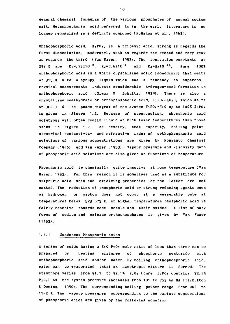
10

general chemical formulas of the various phosphates of normal sodium

salt. Hetaphosphoric acid referred to in the early literature is no

longer recognized as a definite compound CHcHahon et al., 1g63}.

Orthophosphoric acid, HJP04, is a tribasic acid, strong as regards the

first dissociation, moderately weak as regards the second and very weak

as regards

2gs K are

the third C Van Razer, 1 g53). The

Kt=. 75x1 o- 2 , K2 =O. 6x1 o- 7 and

ionization constants

Pure

at

100%

orthophosphoric acid is a white crystalline solid Cmonodinic) that melts

at 315.4 K to a syrupy liquid which has a tendency to supercool.

Physical measurements

orthophosphoric acid

indicate considerable

C Simon & Schultz,

hydrogen-bond formation in

1 g3g). There is also a

crystalline semihydrate of orthophosphoric acid, H3P04•~H20, which melts

at 302.3 K. The phase diagram of the system HJP04-H20 up to 100% HJP04

is given in Figure 1.2. Because of supercooling, phosphoric acid

solutions will often remain liquid at much lower temperatures than those

shown in Figure 1.2. The density, heat capacity, boiling point,

electrical conductivity and refractive index of orthophosphoric acid

solutions of various concentrations are given by Monsanto Chemical

Company c1g4&) and Van Razer c1g53). Vapour pressure and viscosity data

of phosphoric acid solutions are also given as functions of temperature.

Phosphoric acid is chemically quite inactive at room temperature (Van

Razer, 1g53). For this reason it is sometimes used as a substitute for

sulphuric acid when the oxidizing properties of the latter are not

wanted. The reduction of phosphoric acid by strong reducing agents such

as hydrogen or carbon does not occur at a measurable rate at

temperatures below 523-673 K.

fairly reactive towards most

At higher temperatures phosphoric acid is

metals and their oxides. A list of many

forms of sodium and calcium orthophosphates is given by Van Razer

C 1g53).

1. 4. 1 Condensed Phosphoric Acids

A series of acids having a H20: P20, mole ratio of less than three can be

prepared by heating mixtures of phosphorus pentoxide with

orthophosphoric acid and/or water. By boiling orthophosphoric acid,

water can be evaporated until an azeotropic mixture is formed. The

azeotrope varies from g1. 1 to g2. 1% P20, (pure HJP04 contains 72. 4%

P20,) as the system pressure increases from 101 to 753 mm Hg (Tarbutton

& Deming, 1g50). The corresponding boiling points range from g67 to

1142 K. The vapour pressures corresponding to the various compositions

of phosphoric acids are given by the following equation:

11

40

20

0 ~ .... er ::, ,- -20 <C er .... a.. :::;; .... ,-

-40

-100...._ ............. ~ ............. ---__.~ .............. __.. ........ 0 20 40 60 80 100

WEIGHT % H3 P04

Log10 Pmm = 8.&1 -T

Rhere %P20~ lies betReen &O and gs. The boiling point and composition of

vapour over the boiling acid are given by Van Razer c1g53) as functions

of the acid composition. Variation of the heat vapourization with

composition of the acid is also given by Van Razer.

The best knoRn of these condensed acids is pyrophosphoric acid, ff4P201

which has a melting point of 334 K. Once melted pyrophosphoric acid is

very difficult to recrystalize and can take up to several months to

solidify at room temperature. This is due to the decomposition of the

pyrophosphoric acid upon melting (Bell, 1g4Q; Durgin et al., 1g37; Van

Razer, 1 g53). Upon melting, pyrophosphoric acid dissociates into a

mixture Rhich contains orthophosphoric acid and some polyphosphoric

acids. According to Van Razer C 1 g53) this is probably attributable to

the close similarity between the hydrogen-oxygen and phosphorus-oxygen

bonds.

The acids obtained by boiling orthophosphoric acid or adding phosphorus

pentoxide to it, or by melting crystalline phosphoric acid, all belong

to a continuous group of amorphous condensed phosphoric acid mixtures,

which extend from pure phosphorus pentoxide to orthophosphoric acid.

Figure 1. 3 shoRs hoR the orthophosphoric acid fraction decreases as the

total composition is removed from that equivalent to HJP04 (between the

ortho and pyro compositions).

12

100 ---- ... 90 -.... ,, ' Long chains ' 0 80 ' \ (ii>ca. 15)

a: ' 70 ' ' ...J Short chains ' < ' ,<2<ii<ca. 15) ' ... 60 0 Pyre (n•2) ,, ' ... 50 ' w ' C, ' ' < 40 ' ... ' ' z 30 ' ...

' ' (.) a::

20 Ortho (n• l) ' ... ' I>. ........ ... 10

o L ____ J__:J:::======--' 3

(ortho) 2.00 1.67 (pyro) (tripoly)

MOLE RATIO H20/P,05 (proximate composition)

1.00 (meta)

Figure 1. 3 Approximate molecular composition of strong phosphoric acids

in terms of the number, n, of phosphorus atoms in the

molecule-ion.

There appears to be an equilibrium composition mixture of chain

phosphoric acids corresponding to every given ratio of H20 and P205 in

these amorphous compositions. In the range from 72 to 82% P205 the acids

have an oily appearance; in the range from 82 to Sq% P20, they progress

through tar and taffy like stages; and above go% P205 they are brittle

glasses.

Rhen any of the condensed phosphoric acids are dissolved in water,

hydrolysis to orthophosphoric acid takes place. The rate of hydrolysis

is externally dependent upon temperature. At 2gs K the half-life for the

formation of orthophosphoric acid from the condensed form is a matter of

days, whereas at 373 K the half-life is measured in minutes. Because of

the reasonably long life at room temperature, the condensed phosphoric

acids can be studied in aqueous solution at room temperature.

In the manufacture of phosphoric acid from elemental phosphorus three

steps are involved:

1. Burning of the phosphorus

2. Hydration of the resulting phosphorus pentoxide

3. Collection of the mists formed

In most plants the elemental phosphorus is burned as a liquid. Corrosion

is a serious problem in all installations. Details and operating data

from a phosphoric acid plant are given by Striplin c1g48).

The oldest and most economical method for making crude phosphoric acid

is to treat phosphate rock with sulphuric acid, thereby precipitating

calcium sulphate and releasing phosphoric acid. (This is knoRn as the

Ret process.) The phosphoric acid obtained in this way must be purified.

13

Van Razer c1g53) has described a method for determining the total P20,

in any phosphate. Another method is that of the AOAC c1g50).

1.5 PHOSPHORIC ACID AS A CATALYST

Catalytically, phosphoric acid has been used principally for the

polymerization of CJ and C4 olefins ( Langlois, 1 g53). In this regard the

great majority of all commercial polymerization units in the petroleum

industry utilize phosphoric acid as a catalyst (Oblad et al., 1q58;

McMahon et al., 1q63). The most widely used form is the extruded form of

the calcined phosphoric acid and kieselguhr composite developed by

Universal Oil Products Company. Several examples of its use have been

described ( Deeter, 1 g50; Egloff & Reinert, 1 g51; Ipatieff & Corson,

1 q36, 1 q38; Ipatieff et al, 1 g35).

Phosphoric acid, in several forms, can be employed catalytically in a

large number of reactions other than the polymerization of olefins.

There are many patents covering the use of various phosphates as

catalysts in the vapour phase hydration of olefins, with steam, to the

corresponding alcohols.

Dunstan & Howes c1g36).

A list of such patent numbers is given by

One field of organic chemistry in which phosphoric acid, as a catalyst,

finds application is the alkylation of aromatic hydrocarbons by olefinic

hydrocarbons to produce compounds of ~ mixed alkyl-aryl character

(Ipatieff, 1g35 b). One such reaction involves the formation of

isopropyl benzol by the treatment of benzol with propene according to

the following reaction:

Phosphoric acid can also be used to cause condensation reactions between

either ethers or alcohols and aromatic hydrocarbons in which water is

primarily split off to yield olefins. Phosphoric acid may also be used

with olefins in the alkylation of ring compounds containing substituent

groups, notably phenols and amines. Phosphoric acid catalysts in

essentially solid form can also be used in isomerization reactions.

Various phenolic ethers, for example, can be isomerized to the

corresponding alkylated phenols. Another application is tte manufacture

of acid esters from olefins and aliphatic carboxyllic acids according to

the following reaction type:

14

Other examples include miscellaneous types of dehydration reactions upon

aliphatic hydroxy compounds.

An important application involves the treatment of cracked gasoline

vapours ( Ipatieff, 1q35b). By using properly prepared and sized

phosphoric acid-absorbent granules as filler in treating towers, and

temperatures and pressures common to the fractionaters of cracking

plants (3bb K to 473 K and . 71 HPa to 2. 03 HPa), the olefinic

constituents of

either in one,

otherwise appear

these gas mixtures may be selectively polymerized,

or several stages. The gum-forming olefins, which would

in the gasoline from the plant, are converted to high

which are left behind as bottom reflux in the final boiling materials

fractionating step. A certain proportion of the normally gaseous mono-

olefins present is polymerized to form gasoline boiling range liquids of

superior anti-knock value. In this way, both yield and quality of the

gasoline from the cracking process is improved (Ipatieff, 1q35b).

The examples given above are only some of the many possible catalytic

uses of phosphoric acid.

1. 5. 1 Phosphoric Acid as a Polymerization Catalyst

As already mentioned, catalytically, phosphoric acid has been used

principally as a polymerization catalyst in the polymerization of CJ and

C4 olefins (Langlois, 1q53). It has been employed commercially in three

different forms (Langlois, 1q53).

1. A catalyst consisting of a thin film of phosphoric acid supported on

fine quartz sand.

2. A calcined composite of phosphoric acid and kieselguhr.

3. A copper pyrophosphate composition which apparently owes its activity

to a partial conversion to free phosphoric acid.

The calcined composite of phosphoric acid and kieselguhr is the most

active of the catalysts used in polymerization and has the greatest

active surface area C Jones, 1 g5b). This process has been described in

detail by Egloff & Reinert c1q51).

Although there may still be scme units using the copper pyrophosphate

catalyst, its lower activity for the conversion of propene and 2-butene,

which are made in greater quantities by catalytic-cracking units than by

thermal crackers,

solid phosphoric

has caused many of these units to be converted to the

acid catalyst C Jones, 1 g5b). This process is described

15

by Steffens et al. ( 1 q4q). The process was patented by Polymerization

exclusively for non-selective

et al. C 1 q4q) studied the

over copper pyrophosphate

Process Corporation. Its use was almost

polymerization (Sherwood, 1q57). Steffens

effect of process variables on performance

catalyst.

Since the start of commercial polymerization, liquid phosphoric acid on

various supports has been tried, but none has been as successful as the

solid phosphoric type Ckieselguhr) (Jones, 1q56). In 1q37 a commercial

sized unit using liquid phosphoric acid on quartz was built (Langlois &

Ralkey, 1 q51). The advantages of this catalyst are low cost, Ridespread

commercial availability, simplicity of regeneration, high mechanica!

strength and ready adaptability to a variety of feedstocks and types of

service (Langlois & Ralkey, 1q51). In this process the catalyst is made

inside the reaction zone by placing the support (quartz) in the reactor,

filling the reactor with liquid phosphoric acid and then draining off

the excess acid, prior to the introduction of the feed. The catalyst is

replaced by washing off the acid layer and recoating the retained quartz

particles in situ (Sherwood, 1q57). The catalyst can be used over a wide

range of pressure, temperature and water content of the feedstock.

Accidental overhydration does no permanent damage to the catalyst

( Langlois & Ralkey, 1 q51), but ammonia and amines are poisons. Due to

the small surface area of the catalyst support employed, relatively

large reactor sections are required for a given polymer product (Jones,

1 q56) .

Ipatieff (1q35a) used 100% liquid phosphoric acid to polymerize both

propene and butene (Ipatieff & Corson, 1q35a) at a temperatures of up to

477 K and pressures up to 5.06 HPa. Ipatieff & Pines c1q36) polymerized

propene at 605 K to 644 Kin the presence of go% phosphoric acid and

with an initial reactor pressure of 82 atm. Investigators at the

Hassacuesetts Institute of Technology examined polymerization using

liquid phosphoric acid ( 10 to 30%) ( Honroe & Gilliland, 1 q38). They

found that the percentage of higher boiling products increased with

increasing conversion. Investigators at I. G. Farbersindustrie ( I. G.

Farbensindustrie Report) examined the polymerization of propene using

concentrated liquid phosphoric acid at 4. 05 ~Pa and 473 K. In agreement

with Ipatieff, they found that the molecular weight of the polymer could

be varied by varying the acid strength and adding certain metallic salts

to the phosphoric acid. Bethea and Karchmer ( 1 q56) examined the

polymerization of propene using liquid phosphoric acid over a wide range

of temperatures, pressures and acid concentrations. Dunstan and Howes

16

(1g3&) investigated the polymerization action of phosphoric acid and

some of its salts.

1.5. 1. 1 Solid phosphoric acid catalyst (kieselguhr support)

These catalysts are produced by a series of relatively simple steps

comprising (Ipatieff, patent, 1g35b): mixing a liquid phosphoric acid

and adsorbent material (kieselguhr) in selected proportions, heating at

te•peratures of about 453 K to 4g3 K, followed by grinding and sizing to

produce particles of the desired size. The temperatures employed in the

mixing step can range from 3g3 K to 453 K. In this range the acid is

fluid enough to enable rapid mixing by mechanical devices. The

calcination temperatures can range from 453 K to 573 K without damaging

the structure, strength or catalytic efficiency of the particles

produced. The calcination step renders the catalyst solid. Depending on

the calcination temperatures, the calcining period can last from 20

hours up to 60 hours (Ipatieff, 1g35b). The catalyst consists of white

or grey cylindrical-shaped pellets. It is bard when dry, but is

extremely hygroscopic.

These catalysts are poisoned by alkaline materials in the reactor feed.

The most commonly encountered poisons of this type are ammonia and

combined organic nitrogen compounds of a basic nature. Neither oxygen

nor butadiene are classified as catalyst poisons, but their presence in

the feed has a deleterious effect on the catalyst life. The presence of

oxygen results in the formation of long-chained polymers, boiling much

above the gasoline-distillation range. This heavy polymer, or tar,

remains on the catalyst, coating the surfaces and plugging the catalyst

voids. Butadiene over-polymerizes to tar (Jones, 1g56). Host dienes and

acetylenes produce a similar result. Sulphur is a temporary poison

(United Catalysts Inc., operating instructions).

Operating variables of importance include catalyst acid strength,

reaction temperature, pressure, contact time and feedstock composition.

These variables control both the extent of conversion and the quality

and composition of the polymer and are discussed in more detail in

Section 3. 1.S. The kinetics of olefin oligomerization and polymerization

have been studied by Bethea & Karchmer c1q56) using liquid phosphoric

acid, Langlois & Halkey c1g51} using liquid phosphoric acid on quartz,

and Friedman & Pinder (1q71) using solid phosphoric acid. The kinetics

are described in detail in Section 3. 1. 5.

17

Descriptions of the industrial process have been given by McMahon et al.

( 1 %3), Egloff S. Reinert ( 1951), Sachanen ( 1940), Jones ( 195b) and Oblad

et al. ( 1 958) .

1. b MECHANISM AND THERMODYNAMICS OF POLYMERIZATION

1. b. 1 Mechanism of Polymerization

Catalytic polymerization reactions are classified as either free radical

or ionic mechanisms. Ionic mechanisms are further subdivided into

cationic or anionic polymerization.

Examples of free radical catalysts are peroxides. Anionic catalysts are

basic substances such as. metallic sodium. These catalysts readily

dimerize propene to a mixture of double bond isomers of 2-methyl-pentene

at 423-473 K and 7-35 MPa ( Germain, 1969). In this reaction the

carbanium dimer is unstable and in an alkene environment the reaction is

highly selective for dimers.

1.o. 1. 1 Cationic polymerization

Examples of various catalysts in this group are:

TYPE

Acids

Solid oxides

Friedel Crafts

EXAMPLE

Phosphoric acid

Silica-alumina

Aluminium chloride

CHEMICAL

HJP04

Si02 - AhOJ

AlClJ

All these catalysts are acidic in the Bronsted sense. The nature of the

Bronsted acid is dependent on the so called co-catalyst in the case of

Friedel-Crafts and solid oxide catalysts.

Catalyst: AlClJ

Co-catalyst: HCl

Idealized Bronsted acid: CH.)(AlCl4-)

Si02 - AhOJ

H20

CH+) C Al( -0-Si) -t -)

It was shown by Ipatieff and Crosse (1936) that in the polymerization of

ethene over AlClJ, H20 or HCl is essential for polymerization activity.

Similar! Y, with other catalysts, the Bronsted acid forming co-catalyst

is essential for catalyst activity. These catalysts can all generate

carbonium ions in alkenes by adding the proton from the acid to the

extra electron pair in the double bond (pi electrons). From calculations

of proton affinities of C-atoms in the double bond, Evans and Polanyi

18

c1g47) have shown that the proton will add to the end carbon atom, thus

obeying Harkownikoff' s rule in the formation of the carbonium ion.

Thus:

The carbonium ion so generated may add to another alkene, forming a

higher molecular weight carbonium ion. This, in turn, can either add to

further alkenes, or yield its corresponding alkenic polymer by

elimination (usually of a proton). According to HcHahon et al., c1gb3)

five basic carbonium ion reactions summarize polymerization reactions.

1. The carbonium ion may add to an olefin to form a carbonium ion of

higher molecular weight, or the carbonium ion may decompose to form a

smaller carbonium ion and an olefin.

2. The carbonium ion may isomerize by migration of a proton. Tertiary

carbonium-ions are more stable than secondary ions which, in turn,

are more stable than primary ions.

3. The carbonium ion may isomerize by migration of a methyl group.

4. A hydride ion may be abstracted from another molecule or from another

carbonium ion.

5. The carbonium ion may eliminate a proton, forming an olefin.

In addition to polymerization, carbonium ions can also -

Lose a proton either (i) to the catalyst, so regenerating the acid, or

(ii) by transfer to another alkene generating a new carbonium ion.

Add a hydride ion by transfer from a hydrocarbon.

Cause a hydrocarbon to crack.

Cause a hydrocarbon to isomerize.

Lose a hydride ion to become a 'double carbonium ion'. This may cause

further reactions such as cyclization to occur.

After cyclization, the hydrogen thus generated may be used in

saturating other alkenes.

Thus the products of' polymerization' reactions will be complex mixtures

which may include alkanes, alkenes, aromatics and other cyclic

compounds. In addition to these products the catalyst becomes covered in

a layer of coke Ca black, amorphous, organic substance of low hydrogen

content). Due to the extremely complex nature of the products, the term

polymerization must be used with some qualification. Schmerling &

Ipatieff ( 1q5Q) proposed the following definitions:

True polymerization - yields products which consist of alkenes with

molecular weights which are integral multiples

of the monomer alkene.

Conjunct polymerization - yields a complex mixture of alkanes, alkenes,

alkadienes, cyclo-alkanes and alkenes, and

aromatics with the number of carbon atoms not

corresponding to integral multiples of the

monomer.

Copolymerization - inter- or cross polymerization of two or more

different alkenes.

Rith regard to the above definitions, the term oligomerization will be

used in this work to encompass the overall process occurring during a

reaction of the type involved when propene reacts over solid phosphoric

acid catalyst. This is largely true polymerization with some conjunct

polymerization. Also intended by oligomerization is that the polymers

(oligomers) so formed consist of only several monomer units (Germain,

1.6.1.2 Propene oligomerization

Proton addition to the olefin proceeds in a manner which gives the more

stable (secondary) rather than the less stable (primary) carbonium ions

( Hart, 1 qt,4; McMahon et al. , 1 %3).

An isopropyl carbonium ion can react with a molecule of propene to give

a dimeric ion which can loose a proton, in either of two ways, to form

simple propene dimer (McMahon et al., 1q&3).

c-c-c-c+-c C-C-C-C=C I I C C

C-C-C=C-C

I C

McMahon et al. c1qb3) have noted that the dimeric ion may rearrange

before elimination of a proton according to the following:

c-c-c-c•-c I C

20

c-c·-c-c-c

11.

c-c-c•-c-c I C

1l

c-c·-c-c-c I C

I C

1l

c-c=c-c-c I C

1l

C-C-C=C-C I C

1l

c-c=c-c-c I C

1l

C=C-C-C-C I C

C=C-C-C-C I C

Under conditions where propane undergoes oligomerization, trimers are

formed more readily than dimers. Hith solid phosphoric acid catalyst at

433 K and 1 HPa, the products of propane oligomerization consist of

approximately 50% nonenes, 25% dodecenes and less than 5% hexenes

( Schmerling & Ipatieff, 1g5Q). This low yield of hexene can be explained

in terms of the relative stability of the propene dimer and monomer

carbonium ions. The dimer can generate a tertiary carbonium ion which is

more stable than the secondary carbonium ion of the monomer, and will

therefore exist for a longer time before expelling a proton. There is,

therefore, a greater chance for the dimer to further add another

monomer, than there is for monomer dimerization.

c-c· + C=C-C-----+ c-c-c-c·-----+ C-C=C-C-C + H+ I I I I C C C C

c-c-c-c· + c=c-c kp

-----+ c-c-c-c-c-c• l< t

_____. C-C-C-C-C=C-C + H+ I I I I I I I C C C C C C C

The degree of polymerization is related to the ratio (kp/kt) of addition

( propogationl and proton loss (rupture).

kp = rate of further alkene addition (polymerization)

kt= rate of proton expulsion to form an alkane ( termination)

21

The last reaction represents either the return of H+ to the catalyst or

the transfer of H+ to an olefin molecule { Germain, 1 qbq).

Due to isomerization and hydrogen transfer, the polymeric structures do

not correspond to the simple reaction scheme presented above. According

to Germain (1qbq), the dimer, trimer and tetramers of propene, for

example,

isomers):

should have the folloRing structures (Rith double bond

Dimer

Trimer

Tetramer

C-C-C=C-C I C

c-c-c-C-C=C-C I I C C

c-c-c-c-c-c-c=c-c I I I C C C

and double bond isomers

Skeletal isomers Rill, hoRever, be present under most reaction

conditions { Schmerling 8. Ipatieff, 1 q50) and thus, for the propene dimer

{ignoring double bond position),

folloRing possibilities exist:

according to Germain (1qbq), the

C

I c-c-c-c-c c-c-c-c-c c-c-c-c c-c-c-c

I I I I I C C C C C

Trimers and tetramers are very complex mixtures. Trimerization occurs by

addition of propene to dimeric ions. The C9 carbonium ion can rearrange,

resulting in many product structures. The propene trimer may crack to

form non-multiple units of monomer.

Conjunct polymerization, producing saturated and unsaturated products,

can occur by hydrogen transfer when a carbonium ion abstracts hydrogen

from an olefin to produce an olefinic carbonium ion plus a paraffin

C Ipatieff & o· • 1 nes, 1 g30). The olefinic carbonium ions produce

polyolefinic material that fouls polymerization catal~·sts ( Mcllahon et

al. , 1 %3). There is a transition from true polymerization at 366 K to

conjunct polymerization at 561 K ;;i th phosphoric acid ( llcl1ahon et al.,

1Qb3). High acid concentrations also fa,our conjunct pol;m2rization.

The above carbonium ion mechanism p.t'oposed b,; ;lhitmorE ( 1'134) is the

most Ridely accepted for alkene polymerization in heterogeneous

catalysis (Schmerling & Ipatieff,

HcHahon et al. , 1 g63).

22

1 g50; Flor:,:, 1 '16g; Langlois,

The existence of a free alkyl carbonium ion in the same sense as an ion

in solution (Langlois,

investigators prefer

1 g53) has been seriously questioned. Many

a carbonium ion ;,hich is never separated

significantly from the anion of the catalyst, but ~here tha two axist as

an ion pair. There are those rthO prefer to consider an even lesser

degree of charge separation, perceiving the intermediate in terms of a

polarized molecule. For the purpose of explaining the structure of

products formed, the degree of charge separation is insignificant.

This mechanism is different from that postulated b; Ipatieff (1935a) for

homogeneous polymerization

intermediate ester formation.

using phosphoric

1. 6. 1. 3 Butene oligomerization

acid, ;; hi Ch i n-; 0 l 'i e 5

It has been sho,rn C McCubbin 8. Adkins, 1 g30; :{hi tmore 3. Church, 1 g32), in

the polymerization of iso-butene, that the t;;o octanes, namel/ 2, 4, 4-

trimethyl-1-pentene and 2,4,4-trimethyl-2-pentene, are produced in the

ratio of about 4: 1 in the presence of dilut.:: sulphut'ic c1cid. This is

representative of several acid catalysts c:chmcrlini & Ipatieff, 1g50J.

The sequence is illustrated by the follo~ing equations:

C C I I

c=c + g• ___. c-c· I I

C C

C I

c-c• + C=C-C ___. I

C

C

I C

I • c-c-c-c -c I I C C

32%

13%

C I

c-c-c-c•-c I I C C

C I

' C-C-C-C=C + !I+ I I I

C C

C

C-C-C=C-C ~ H+ I !

C C

23

2,4,4-trimethyl-1-pentene is formed in larger amounts since the

elimination of a proton from the methyl group adjacent to the electron

deficient carbon atom, occurs more readily than from the neopentyl

system (Schmerling & Ipatieff, 1g50). The structure of these two isomers

was proved by ozonation by HcCubbin & Adkins c1g30).

In addition, whereas there are only two protons in the methalene group

of the neopentyl system, there are six hydrogens attached to the methyl

carbons. The eliminated proton can add to the reaction chain. The

relative difficulty of removing a proton from the neopentyl group has

been illustrated (Rhitmore et al., 1g42). Trimers are formed mostly by

reaction of the t-butyl carbonium ion with the dimers, and partly by the

reaction of the iso-octyl carbonium ion with the monomer (Rhitmore &

Church, 1g32; Rhitmore et al., 1g41).

The carbonium ion formation is directly related to the proton affinity

of the olefin (Germain, 1gog), hence the higher reactivity of iso-butene

when compared to that of the n-butenes, propene or ethylene. The isomers

present in the trimerized isobutene product have been examined by

Rhitmore et al. c1g41) and HcCubbin c1g31). A summary of their findings

is given by Schmerling & Ipatieff c1gso> and Oblad et al. c1g58).

In addition to polymerization, phosphoric acid causes considerable

isomerization with the butenes. Hence in many instances the material

which was actually polymerized might have been a mixture of the isomeric

butenes, the relative amounts of which would depend upon the

experimental conditions.

Little work has been carried out on the polymerization of 1-butene and

2-butene (the chemistry of petroleum derivatives). Schmerling & Ipatieff

c1g501 have listed the dimerized products obtained when sec-butyl

alcohol is treated with sulphuric acid at 353 K under pressure. The

dimerized and trimerized products obtained when 2-butene is polymerized

in the presence of activated floridin have also been described

(Scbmerling & Ipatieff, 1g50). The trimerized products were explained

using the carbonium ion mechanism.

Schmerling & Ipatieff (1g50) have reviewed possible mechanisms and the

products obtained from the polymerization of several methyl butenes

(pentenes), dimethylbutenes and the polymerization of mixed olefins

Ce.~. CJ and C4). The products and mechanisms will not be discussed.

24

1.&.2 Thermodynamics of Alkene Oligomerization

Oblad et al. c1q58) have examined the thermodynamics of oligomerization

of gaseous mono-alkenes to gaseous alkene products. Phase changes and

deviations from ideality were ignored.

Figure 1.4 (taken from Oblad et al.) shows the free energy change during

dimerization of C2 through C6 mono-olefins as a function of temperature.

(The lines for C4 and c, which are not shown are almost superimposable

on the C6 line). Mote that the free energy change for the dimerization

of propene to trans 3-methyl-2-pentene is greater than that for the

dimerization to the terminal olefins( F,~ure. t.5').

The former (isomers of the corresponding higher olefins) are always the lowest

structures of aisRe&t energy. The equilibrium conversion, therefore, of

an alpha olefin to a high alpha olefin, will always be less than the

corresponding conversion of an alpha olefin to an iso-olefin.

200 ,oo 600 300 1000

Figure 1. 4 Free energy change during dimerization

25

For comparative purposes, the equilibrium conversion as a function of

temperature and pressure is shown in Figure 1. 5 for the following

dimerization reactions:

2CJ (g) ----+ 1-hexene Cg)

2CJ Cg) ----+ trans-3-methyl-2-pentene Cg)

These gas phase reactions provide only limited information on 2-phase

heterogeneous reactions. Dimerization of beta olefins or iso-olefins to

the corresponding higher olefins will be similar to the alpha olefin -

alpha dimer relationship. The dimerization of beta olefins or iso

olefins to alpha olefins is always favoured.

In the production of polymers greater than dimer from alpha olefins, the

free energy versus temperature curves fan out from a constant point

( Oblad et al., 1 g58) at a temperature between 500 and 600 K. This is

100.0

.. z ao.o 0

(J)

0::::: w so.a > z 0 U 40.0

co

_J

::i 0 w

20.0

a.a

a.a

FIG 1 . 5

2.0

HEXENE (!):400 K ~=500 K +=600 K X:700 K

4.0

TRANS-3-NETHYL-2-PENTENE ~=400 K 'I> =500 K ~=600 K 2=700 K

6.0 8,0

PRESSURE, MPR FOR PROPENE

ANO EQUILIBRIUM CBNVERSIBN DIMERIZRTIBN TB 1-HEXENE TRRNS-3-METHYL-2-PENTENE

IO .Q

illustrated for propene in Figure 1. 6 for the polymerization to higher

terminal olefins.

Hith respect to the free energy changes in the polymerization of propene

and 1-butene, the free energy change of adding a monomer to a growing

2b

chain seems to remain constant after the dimer has formed (Oblad et al.,

1qs8>. This is illustrated in Table 1. 4.

Table 1. 4 Standard free energy change (kcal) of polymerization per

monomer unit added.

CJ C4

Temp I Dimer Trimer Pentamer Hexamer Dimer Tetramer Pentamer

2q8. 1 -q. 18 -q. 01 -8,q3 -8. q2 -q.s -q.22 -q, 17

bOO 1. 2 1. 5 1. E>S 1.t,q 1. 2 1. &3 1. 71

goo 10. q 11. 45 11. 7 11. 7b 11. 5 12. 1 12. 15

- •o

•oo soo 1000

Figure 1. b Free energy changes for the polymerization of propene

Taking a single olefin species, such as propene, the free energy change

for the formation of the higher polymers can be estimated theoretically

from the corresponding energy of dimerization (Oblad et al., 1q58). The

free energy change per mole of monomer for the higher polymers should

approach twice the change for the dimer formation (provided heat and

entropy effects are constant) and hence the higher oligomers are

27

favoured over the dimer. Oblad et al. c1q58) note that, up to the

formation of c, hexamer, the heat of reaction folloRs the theoretical

relationship more closely than the free energy change, indicating that

the entropy change is not constant up to the hexamer formation. They

suspect, hoRever, that the free energy change Rould approach the

theoretical value for polymers higher than n=o.

1.7 REACTORS FOR DETERMINING THE KINETICS OF HETEROGENEOUS CATALYTIC

REACTIONS

1. 7. 1 Background

The choice of a suitable reactor for carrying out experiments under

conditions Rhere meaningful kinetic rate expressions can be obtained, is

of great importance, and depends on the objectives of the research

(Cooke, 1g7q). This is particularly true of catalytic reactions in which

external and pore diffusion resistances are important. Radial and axial

transport effects in the reactor must be accounted for. The choice of a

laboratory catalytic reactor must therefore be made on the basis of

several considerations (DoraisRamy & Tajbl, 1q74; Reekman, 1q74).

The central problem in obtaining kinetic data from any reactor is to be

certain that one is evaluating the rate of the intrinsic chemical

reaction on the catalyst surface (Cooke, 1q7q). The measurement of the

rate of chemical reaction occurring on the surface of a catalyst is made

in terms of bulk concentrations and temperatures. For these bulk

concentrations to reflect the chemical kinetics accurately, there must

be an absence of concentration gradients betReen the bulk gas phase and

the catalyst surface. Reactions Rhich are affected by gas-film

resistances show very marked deviations from their true rates because of

the poor heat transfer across the stagnant gas film and the exponential

dependence of the rate on temperature (Cooke, 1g7g).

Concentration gradients can also occur inside the pores of a catalyst

particle. This is called pore-diffusion resistance. Similar to gas-film

resistance, the absence of concentration and temperature gradients

inside the catalyst pores is essential for the intrinsic kinetics to be

measured.

There are many laboratory reactor types. A list of the more common types

is given beloR:

28

- differential reactor

- fixed bed reactor

- stirred batch reactor

- stirred-contained solids reactor

- continuous stirred tank reactor

- straight through transport reactor

- recirculating transport reactor

- pulse reactor

A summary of the ratings of the reactors for sampling and analysis,

isothermality, residence contact time, selectivity disguise-decay and

construction problems is given in Table 1.5 (Reekman, 1g74). The ratings

are specific to a three-phase system with a powdered decaying catalyst.

The interpretation of the ratings for other systems is straight

forward.

Advantages and disadvantages of many laboratory catalytic reactors have

been widely reported (Doraiswamy & Tajbl, 1g74; Christoffel, 1g82;

Reekman, 1 g74).

Table 1. 5 Summary of laboratory reactor ratings.

Reactor

type

Sampling

and

analysis

a. Differential P-F

b. Fixed bed G

C. Stirred batch F

d. Stirred cont. G solids

e. C. S. T. R. F

f. Straight F-G through transport

g. Recirculating F-G

b. Pulse G

p = Poor F =

Iso- Residence Selectivity

therm- contact disguise-

ality time decay

F-G F p

P-F F p

G G p

G F-G p

G F-G G

P-F F-G G

G G G

F-G p F-G

Fair G = Good

Construction

problems

G

G

G

F-G

P-F

F-G

P-F

G

1. 7. 2 Gradientless Reactors

Gradientless reactors are those reactors that are capable of performing

at, or close to, gradientless conditions, where there are no external

catalyst heat or mass transfer limitations (Kuchanski & Squires, 1q?b).

There are many versions of this reactor type. Two well known examples

are those of Carberry C 1 qb4) and Berty ( Berty et al. , 1 qbq; Berty, 1 q74).

In the famous Carberry reactor the catalyst is mounted on the agitator

(inside the reactor) and the high rotational speeds provide good

catalyst-fluid contact. In the Berty type the catalyst is held

stationary and the fluids are internally recycled through the catalyst

bed by means of an internal blower. Sampling and analysis of the product

composition of these reactors present no problems. Good mixing is

possible and isothermality should be achieved. Residence times can be

measured accurately. These reactors are difficult to construct. There

are many examples of these reactor types (Carberry, 1qb4; Tajbl et al.,

1qbb, 1qb?; Tajbl, 1qbq a, ~ Garanin et al., 1qb7; Brown & Bennett,

1 q70; Berty et al., 1 qbq; Berty, 1 q74; Li vbjerg & Villadsen, 1 g71;

Mahoney, 1q74; Choudhary & Doraiswamy, 1q72; Perkins & Rase, 1q58;

Satterfield & Roberts, 1qb8; Butt et al., 1qb2; Leinroth & Sherwood,

1qb4; Ford & Perlmutter, 1qb4; Relyea & Perlmutter, 1qb8; Brisk et al.,

1 qf>S; Barcicki et al., 1 qs1; Caldwell, 1 q83; Ke-Chang & Nobile, 1 q8b). A

good review of these reactors has been given by Bennett et al. (1q72).

Hany of these reactors have some outstanding features for a particular

application, but only those with centrifugal internal blowers can assure

steady state operation (Berty, 1q84). Of these, very few permit the

close estimations of internal flow, and hence, of the heat and mass

transfer conditions at the catalyst (Berty, 1q74).

1.7.2. 1 Recycle reactors

Reactors that are simple in construction, such as fixed bed and

adiabatic reactors, approach their ideal conditions in commercial size

rather than on a lab scale. On a small scale they are handicapped by

significant temperature and concentration gradients that are not even

well defined. In contrast, recycle reactors and CSTR' s (continuous

stirred tank reactors) in general come much closer to their ideal state

in small sizes C Berty, 1 qg4).

All recycle reactors and CSTR' s may be regarded as differential reactors

( Jankowski et al, 1 q78; Berty, 1 qg4). The purpose of a recycle reactor

can be deduced from a differential reactor if one considers that, close

30

to the ideally small conversion, the feed has almost the same

concentration as the discharge. (Remember that in all CSTR' sand recycle

reactors, the reaction takes place at the discharge conditions, or ?ery

close to them.) Just enough fresh reactants can be added to make up for

the chemical change and for the reactants lost in the exit stream. This

eliminates the analytical problems with the once through differential

reactors (Berty, 1q84). There are many published examples of the more

common laboratory recycle reactors (Carberry, 1qb4; Brisk et al., 1qb8;

Taj bl et al. , 1 %b; Bennett et al. , 1 q72; Ha honey, 1 q74; Berty, 1 q74;

Berty, 1q77; Robinson & Mahoney, 1q77; Mahoney et al., 1q78; Hyers &

Robinson, 1 q7s; Berty, 1 q7q; Barcicki et al., 1 q81; Gangwal, 1 q82; Ke

Chang & Nobile, 1 gab; Caldwell, 1 qs3).

Internal recycle systems, which approximate CSTR behaviour, are probably

the most useful reactors for obtaining catalytic kinetic data, since

external circulation is plagued by mechanical pumps and the need to cool

and reheat

al., H78).

the recycle

the recycle stream, resulting in poor operation (Mahoney et

CSTR behavior can be achieved in a recycle reactor only if

ratio is greater than 25 (Carberry, 1qb4). An overview of

recycle reactors has been given by Berty (1q84).

1. 7.2.2 The internal recirculation type gradientless reactor (internal

recycle reactor)

The internal recycle reactor (fixed basket) was developed by Berty at

Union Carbide in the early 1qbQ's. At that time little interest was

shown in the new reactor type. Some years later interest bad developed

and by the late 1q7o•s the use of recycle reactors was commonplace

(Berty, 1q84). A review of many internal recycle reactors is given by

Jankowski et al.(1g78). An example of a standard Berty type gradientless

(fixed basket, internal recycle) reactor is shown in Figure 1. 7.

The most significant advantage of this reactor type, as previously

mentioned, is the removal, to a large extent, of mass and heat transfer

gradients. Since the reactor permits reaction studies at isothermal

conditions with uniform concentrations, it eliminates the need for the

solution of partial-differential equations. Each steady state experiment

yields a reaction rate that is calculated from the ordinary mass balance

equations for a CSTR ( Mahoney et al., 1 q78):

ff

F =

Io - Xi

31

No 1

Drott Tube

Fillar Ring

Impeller

Figure 1. 7 Standard Berty type internal recycle reactor (fixed basket)

C Berty, 1 g74).

Rhere R :: mass of catalyst

F :: molar feed rate of catalyst

I1 :: inlet concentration of reactant

Io :: outlet concentration of reactant

r, :: global rate of reaction per unit mass of

catalyst

These reactors can be problematic in studies Rhere the reaction products

are qualified by some practical tests ( Berty, 1 g94). Examples include:

1. The production of

plasticiser alcohols,

polymer olefins for subsequent conversion to

Rhere the product quality is tested after one

or more reactions, and no exact relationship for quality can be

expressed.

2. The conversion of a complex natural product into a partially modified

material that is used for an empirically defined purpose, such as a

thickener.

3. Rhen there is a possibility of homogeneous reactions in the empty

spaces of the reactor.

4. Rhen reactions on the Ralls of the reactor are a possibility.

32

In summary, internal recirculation reactors are highly suitable for

catalyst testing and kinetic studies (Berty, 1g84).

1. 7. 2. 3 Examples of the use of gradientless reactors to obtain kinetic

data

There are many examples of the use of these reactors to obtain intrinsic

kinetic data. Taj bl et al. ( 1 gt,t,) demonstrated the operability of the

'Carberry reactor' by examining the palladium-catalyzed oxidation of CO

Ri th 02. Mahoney ( 1 g74) used a Berty type ( fixed bed) reactor to

determine the kinetics of ultraforming. Ultraforming, Rhich is a high

severity catalytic naptha reforming process, operates at high

conversions, and the catalyst deactivates rapidly betReen regenerations.

Mahoney concentrated on the reactions of n-heptane catalyzed by a

commercial platinum-on-alumina catalyst Rhich had been activated by a

halide promoter. Berty ( 1g74) used his noR famous internal recycle

reactor to study the kinetics of ethylene hydrogenation on HarshaR 3210-

T catalyst.

found that

He also examined the

a catalyst Rhich had

oxidation of propene to acrolein and

previously been discarded (based on

fixed bed laboratory reactor studies) was dramatically more active than

the catalyst Rhich had been chosen as the most active.

Robinson & Mahoney (1g77) designed an internal recycle reactor to study

the multiphase coal hydroliquefaction process. They successfully tested

various catalysts for short term ageing behaviour, in the absence of

transport limitations. Hyers & Robinson (1g7g) used a similar reactor to

study the kinetics of the three phase dibenzothiophene desulphurization.

Their results compared favourably Rith those performed in a trickle bed

reactor by Frye and Hosby c1gt,7)_ Caldwell (1g83) studied the kinetics

of the dehydration of ethanol in his modified version of Berty's

internal recycle reactor. Carberry et al. ( 1 g85) recently developed an

internal recycle (Carberry type) reactor that permits the accurate

determination of intrinsic kinetics for three-phase systems. Their

reactor is based on a gas-liquid reactor (Hanor & Schmitz, 1g84), in

Rhich a multiblade rotor creates a thin film of liquid on the

cylindrical Rall. Ke-Chang & Nobile ( 1 ggt,) studied the intrinsic

kinetics of S02 oxidation on a commercial vanadium catalyst. Their study

concentrated on the construction of a Berty type reactor and an

extensive characterization of the reactor. Berty (1g7g) has given some

very useful hints and methods that can be used in the testing of

commercial atalysts in recycle reactors. Santacesaria & Carra ( 1 g33)

studied the kinetics of steam reforming methanol, catalyzed by a

33

commercial Cu-Zn catalyst, in a Berty type reactor. They modelled the

kinetic data according to a Langmuir-HinshelRood model.

1. 8 OBJECTIVES OF THE PRESENT STUDY

The objectives of this Rork are to study, inter alia, the kinetics of

the oligomerization of CJ and C4 alkenes over phosphoric acid on

kieselguhr using an internal gas recirculation reactor, to obtain

satisfactory rate equations and to test these equations on the

performance of an integral reactor. In addition to the characterization

of the reactor system (Rith respect to transport effects) and the

kinetic study, the oligomerization of CJ, C4, c, and mixtures of these

alkenes is studied using pulse reactor techniques.

The reactor system is characterized Rith respect to both mass and heat

transport and residence time characteristics.

Rate equations

alkenes and

are developed

proposals

oligomerization of

kiesulguhr.

made

and

for the oligomerization of the CJ and C4

regarding the mechanism of the

c, alkenes over phosphoric acid on

The rate equations are used to predict the results from an integral

reactor and these results are compared to the actual results obtained.

34

2. MICRO-CATALYTIC PULSE REACTOR STUDIES

2. 1 INTRODUCTION - LITERATURE REVIER

2. 1. 1 Background

The pulse microcatalytic technique has established itself in the field

of heterogeneous catalysis as an important analytical tool (Verma &

Kaliaguine, 1g73). Pulse reactors bave become almost standard equipment

for rapid catalyst screening in tbe petroleum industry and bave found

extensive application for fundamental reaction mechanism studies in both

industrial and academic catalytic laboratories (Galeski & Hightower,

1g70). The technique bas found very useful applications in situations

where either the reactants or the catalysts are in short supply, or are

too expensive to be used in a steady state flow reactor (Verma &

Kaliaguine, 1g73).

2. 1. 2 Pulse Reactor Types and Techniques

There are at least two types of pulsed catalytic reactors (Galeski &

Hightower, 1g70). They are:

1. Chromatographic column reactors.

2. Pulse systems in which the reactor bed and chromatographic column are

independent.

In the chromatographic column reactor, the catalyst also serves as a

partitioning column to separate the products and the reactants (Langer

et al., 1gog). In most pulsed catalytic reactors, some degree of elution

Rill occur.

There are many systems in which the reactor bed and chromatographic

column are independent. The simplest form of microcatalytic pulse

reactor is a gas chromatograph with a small, tubular fixed-bed catalytic

reactor placed in the carrier gas stream between tbe sampling valve and

tbe partitioning column. The reactant slugs are introduced via the

sampling port, mixed with the carrier gas and carried through the

catalyst bed. On their exit, the reactants and products are separated

immediately in the partitioning column and detected by an appropriate

detector (flame ionization or thermal conductivity).

35

This system has severe limitations. The reaction pressure and the

contact time with the catalyst are limited. To avoid this, the carrier

gas can be split into two streams one stream operating under

chromatographic conditions and the other under variable conditions.

Generally in these systems the reactants and products are separated from

the carrier gas by freezing in traps. Effective trapping is sometimes

very difficult. Igarashi & Ogino c1q82) and Steingaszner & Pines c1qob)

have developed useful high pressure catalytic pulse reactors.

A common gas pulse injection is by •eans of a hypodermic syringe into a

T connection, in the carrier gas stream. Small amounts of air accompany

such injections (Galeski & Hightower, 1q70). By-pass dosing systems

avoid this problem. For a fixed doser volume, a known amount of reactant

can be injected by adjusting the doser pressure at a fixed temperature.

Liquids are often pulsed by saturating them in a separate carrier gas

stream, a portion of which is trapped and sent into the reactor.

The most

The bed

common reactor is a

length is generally

tube containing a centered thermocouple.

greater than the diameter to avoid

channelling, and all contacting lines have as small diameters as

possible to minimize dispersion. Several pulse techniques (Scott &

Phillips, 1q8Q) are described below.

2. 1.2.1 Elution with reaction

In this technique a small sample is injected into a gas stream at the

beginning of the column. Using the catalyst as column material results

in a chromatogram with information about the reaction occurring on the

column. Information about the adsorption of the sample molecules on the

catalyst surface can be obtained from the shape and retention time of

the eluted peak of unreacted sample.

2. 1. 2. 2 Hicrocatalytic technique

This classical technique has been described by Kokes et al. c1q55), The

system would consist of a reactor containing a small amount of catalyst

through which a pulse of reactant in a stream of carrier Bas is passed.

The analysis is usually performed on a gas chromatograph.

2. 1.2. 3 Deuterium exchange

Rith this technique, which is an application of 2. 1. 2. 1 or 2. 1.2.2, a

small sample of deuterium is injected into a hydrogen carrier gas stream

36

passing through the catalyst and its emergence is followed by a

katharometer. The retention of the deuteriu• measures the exchange of

the deuterium with adsorbed hydrogen, water and hydrocarbons.

2. 1. 2. 4 Reactor-stop technique

This system is similar to (3) above but here the reactant is stopped on

a longer reactor for varying periods of time and then swept off with the

products to the GC column.

2. 1.2.5 Stopped-flow technique

This is a variation of (1) above in which the gas flow through the

reactor column is stopped from time to time so that the chromatographic

process is switched off, while the reaction is allowed to continue. Mith

each restart of the gas flow, sharp chromatographic peaks are generated

on top of the normal "reaction" chromatogram, each peak corresponding to

one volatile product of the reaction formed during the stop period.

2. 1. 2.6 Sample vacancy technique

Reactant is carried continuously through a reactor and GC column.

Periodically, feed samples are switched into the gas flow between the

reactor and GC columns, generating a differential chromatogram, in which

the positive peaks measure the amount of reactant which has reacted, the

negative peaks the amounts of the various volatile products and the

difference the amount of involatile product.

2. 1. 2.7 Heater displacement technique

Samples, here, are driven through the catalyst by means of a carrier gas

and an external moving heater.

2. 1. 3 Analysis of Pulse Reactor Data

The theory of chemical processes in micro-catalytic pulse reactors can

be classified into two main groups (Yanovskii & Berman, 1972). The first

involves the rapid attainment of adsorption equilibrium, and the second

takes into consideration the rate of attaining equilibrium between gases

and solids. Host research has been

isotherms, but some research showing

reported (Hattori & Murakami, 1968).

concerned with linear

non-linear isotherms

adsorption

has been

37

The nature of adsorption equilibria and the kinetics of adsorption have

a different effect on the degree of conversion, depending on the

reaction order and its specific mechanism (Yanovskii & Berman, 1g72).

The simultaneous treatment of adsorption kinetics and the longitudinal

and internal diffusion involves considerable mathematical difficulties.

Hattori & Murakami c1g74) have emphasized that the pulse reaction

kinetics, coupled with an irreversibly adsorbed reactant, may be

significantly different from that with the reversible adsorption.

Rhen investigating reversible reactions in a micro-catalytical reactor,

some of the features responsible for the rate of a heterogeneous

reaction must be taken into account (Yanovski & Berman, 1g72). Probably

the most important factor is the possibility of separating reactants and

products on the catalyst layer during the reaction.

2.1.3.1 Reactions of the type A~ B

The difference in the adsorption coefficients of A and B will cause the

rate of the reverse reaction to decrease. The same effect is possible as

a result of diffusion when the adsorption coefficients of A and Bare

equal (Berman et al., 1g7Q).

2. 1. 3. 2 Reversible reactions of the type A B + C

For reactions of this type, spatial separation of Band C will induce a

change in the degree of conversion of A as a result of partial or full

inhibition of the reverse reaction CRoginskii et al., 1go1).

2. 1.3.3 Consecutive reactions

For those of the type A+ B ~ R

R + B ~ S

the separation of B and R will result in a decrease in the yield of S

and in an accumulation of the intermediate product R (Hattori &

Murakami, 1go8; Murakami et al., 1go8). This effect depends on the pulse

width at the inlet, as its decrease intensifies separation (Yanovskii &

Berman, 1g72). In the case of a reaction of the type A~ Rand 2R ~ s,

such an effect can arise from the difference in the adsorption

coefficients of reactant A and the intermediate product R.

Rhen the rate at which adsorption equilibrium is reached is slow, the

difference between th& results obtained by pulse and flow methods will

38

be even greater because of the different degrees of catalyst surface

coverage.

Host catalysts require an induction period before exhibiting a constant

level of activity. Hall and Emmett (1959) have found, in the

hydrogenation of ethylene, that the activity on their copper-nickel

alloy catalyst increased strongly with increasing slug number, when the

catalyst was treated in flowing helium for 30 minutes at 3oo'c.

S0meti11es the results obtained with the pulse technique are

significantly different from those obtained with the continuous flow

technique. Hattori & Murakami (1974) found that the main difference

between the two techniques was primarily due to the separation between

the components in the catalyst bed and from the lowering of the

concentration due to the broadening of the pulse. They found that the C

effect of those factors was dependent on the pulse width. They also

noted that the results in the pulse technique approached those in the

continuous flow technique with an increase in the pulse width (the

continuous flow technique corresponds to the pulse technique with an

infinite pulse width). Another way to reduce the difference between the

two techniques is to reduce the contact time (Hattori & Murakami, 1973;

Toyota & Echigoya, 1gb8). Hattori & Murakami (1973) noted, however, that

the above cannot be applied to all reactions.

Basset and Habgood (19b0) showed for first order reactions that

quantitative analysis was possible. However, they used a relatively

simple reaction where the rate of adsorption had to be fast relative to

the rate of the surface reaction. The adsorption isotherm was assumed to

be linear. Their analysis was made possible by the fact that, although

the reactant partial pressure varied from point to point through the

reactant pulse, for first order reactions the fractional conversion of

reactants to products was independent of pressure.

Gaziev et al. (19b3) extended the work of Basset and Habgood to

non-first order kinetic equations, using square and triangular input

pulses having no axial dispersion. The equations used were confirmed

experimentally by Schwab & Ratson (19b5). Bett & Rall (19b8), however,

found a difference between the results obtained from the micro-catalytic

technique and the flow technique for a zero order reaction. Blanton et

al. (19b8) and Hakar & Harrill (1972) extended the pulse technique to

more general cases of non-first order kinetics. They neglected the pulse

dispersion by introducing a dispersion column upstream of the catalyst

bed. The Gaussian-shaped pulse was made broad enough so that it could be

assumed that axial dispersion in the bed had a negligible effect on the

width of the peak. Verma & Kaliaguine c1q73) continued this approach

with a further simplification in their study of the oxidation of

ethylene over a silver catalyst. They reduced the ratio of catalyst bed

length to total pulse length so that the reactant concentration could be

considered to be constant over the entire length of the bed. They

ensured that conversion over the bed was differential. Their results,

which agreed partially with those of their flow experiments, showed that

one of the major drawbacks of the pulse technique as a quantitative

kinetic tool was the need for an instantaneous attainment of adsorption

equilibrium. Sica et al. c1q78) found reasonable agreement between

kinetic parameters, based on

models, obtained from pulsed

power-law and Langmuir-Hinshelwood rate

and steady state flow experiments for the

hydrogenation of benzene on a nickel catalyst.

2. 1. 4 Advantages and Disadvantages of the Pulse Technique

Hicropulse reactors are useful tools with which to investigate

heterogeneously catalyzed gas-phase reactions. These devices can be

complex or surprisingly simple depending on the results desired and the

resources available (Reichle, 1q81). The insight obtained from these

reactors should supplement, not replace, that obtained from steady state

kinetics ( Bett & Hall, 1 qE,8). There are many advantages and

disadvantages associated with the use of micro-catalytic pulse reactors.

The most important are listed below.

Advantages 1. Activity and selectivity data can be obtained rapidly

(Reichle, 1q81; Hall & Emmett, 1q5q),

2. Unlike steady state flow reactors, hot-spots do not

occur C Reichle, 1 qs1; Hall & Emmett, 1 q5q).

3. Extremely small amounts of both catalyst and feed can

be used (Verma & Kaliaguine, 1g73).

4. Qualitative analysis for linear processes is rapid and

relatively simple C Hall & Emmett, 1 g5q).

5. It is a simple technique to use for catalyst life

experiments C Reichle, 1 g91).

Disadvantages 1. For quantitative analysis of results, knowledge of the

adsorption characteristics are essential (Hattori &

Hurakami, 1 g74).

2. The catalyst is generally in an unstable condition

( Reichle, 1 g91; Hall et al., 1 goo).

2. 1. 5

40

3. Steady state is generally not obtained with respect to

adsorption of the gases (Hall et al., 1g&o).

4. Due to the unsteady state conditions that generally

prevail, quantitative analysis is extremely difficult

(Verma & Kaliaguine, 1g73).

5. Results obtained very often differ from those in

continuous systems. This is especially so for non

linear systems (Reichle, 1gs1; Murakami et al., 1gb8).

Applications of the Pulse Technique

The pulse micro-catalytic reactor has had extensive use in the field of

heterogeneous catalysis since its introduction. Up until 1g&o this

technique was used only as a qualitative tool (Keulemans & Vogue, 1g5g;

Hall & Emmett, 1g5g; Hall et al., 1g&o).

Bassett and Habgood (1gbQ) were the first to quantitatively analyse the

results fr_om a pulse system in their study of the catalytic

isomerization of cyclopropane. Steingaszner and Pines (1gbb) designed a

novel high-pressure pulse micro-reactor that could withstand pressures

of up to 70 atmospheres.

Blanton et al. (1gb8) used the pulse micro-catalytic reactor to

quantitatively solve non-linear rate equations in their study of the

hydrogenation of etl.ylene over alumina. Since then many researchers have

quantitatively analysed their pulse reactor data (Bett & Hall, 1gb8;

Murakami et al., 1g&8; Suzuki & Smith, 1g71; Yanovskii & Berman, 1g72;

Verma & Kaliaguine, I g73; Sica et al., 1 g78)

In an effort to extend the quantitative application of the pulse

micro-catalytic reactor to as many linear and non-linear systems as

possible, several authors have rigorously analysed the chemical and

physical processes encountered (Masamune & Smith, 1gb4; Roginski &

Rozental, 1 gt,4; Kubin, 1 g&5; Kucera, 1 g&5; Kocirik, 1 g&7; Denisova &

Rozental, 1g&7; Padberg & Smith, 1gb8; Murakami et al., 1gb8; Schneider

& Smith, 1 gt,8; Adrian & Smith, 1 g70; Suzuki & Smith, 1 g71; Hattori &

Murakami, 1 g73; Hattori & Murakami, 1 g74; Furusawa iat al. , 1 g7b;

Igarashi & Ogino, 1 g82).

Despite the simplicity and speed of operation of pulsed micro-catalytic

reactor systems, the complexities encountered in the quantitative

41

analysis of results remain a severe drawback. Their versatility lies in

their use as a qualitative tool.

2. 2 OBJECTIVES OF THE PULSE HICRO-CATALYTIC STUDIES

The primary objective of the pulse micro-catalytic studies is to examine

the relative reactivities of various hexene isomers over solid

phosphoric acid. Due to the extreaely high cost and limited

availability, the hexane isomers can not be polymerized using a

continuous flow or batch reactor. The only convenient reactor which can

handle extremely small quantities of reactants is the pulse

micro-catalytic reactor.

The second objective is to compare the reactivities of the hexene

isomers with those of propene, 1-butene and iso-butene and to examine

the effect on the reactivities and selectivities of mixing these

reactants. It is also hoped to obtain a better understanding of the

basic reaction pathways followed in the polymerization of the above

feeds tocks.

The objectives of this study may therefore be listed as follows:

1. To investigate the relative

isomers:

reactivities of the following hexene

1-hexene

2-methyl-1-pentene

2-methyl-2-pentene

3-methyl-1-pentene

3-methyl-2-pentene

4-methyl-1-pentene

Cis-4-methyl-2-pentene

2. To compare the reactivities of the above-mentioned hexene isomers

with those of propene, 1-butene and iso-butene.

3. To investigate the effect of mixed feedstocks on the reactivities

and selectivities of the individual reactants.

4. To obtain a better understanding of the major reaction pathways

followed in the polymerization of the propene, butene and hexene

feedstocks.

42

5. To determine, if possible, which of the folloRing reaction sequences

is the most dominant in the production of the C12 oligomer:

CJ + C9----+ C12

C& + C&----+ C12

2. 3 EXPERIMENTAL APPARATUS AND PROCEDURE

2.3. 1 The Pulse Technique Used in this Study

The micro-catalytic pulse technique used in this study was based largely

on that used by Igarashi & Ogino c1g82). The high pressure requirement

of this work did not permit the use of a chromatographic column reactor,

due to the maximum permissible pressure of the gas chromatograph' s

carrier gas. Similar to the system used by the above-mentioned workers,

the high pressure was maintained by an independent, inert carrier gas.

Unlike their system, the reaction products, with the inert carrier gas,

were passed through a gas sampling valve, enabling the analysis of

discrete sample slices. The most serious disadvantage was that, with the

analysis of discrete sample slices, the possibility existed of not being

able to obtain a representative analysis of the entire exit pulse. It

will be shown that this problem Ras overcome.


The reactor system used for the micro-catalytic pulse experiment is

shoRn schematically in Figure 2. 1.

Nitrogen, which Has used as the inert carrier gas, Ras fed to the system

from a high pressure cylinder. The inlet pressure was controlled by

means of a regulator on the nitrogen cylinder. The nitrogen was bubbled

through a temperature controlled water bath. The temperature of the

water bath determined the partial pressure of the water in the nitrogen

stream and, therefore, the acid concentration ( % HJP04) on the catalyst,

at a given pressure and nitrogen floxrate. The xater vapour content of

the nitrogen str~am xas accurately determined by passing a bleed from

the inlet nitro;~n strsam o~er an aluminium oxide sensor. The sensor

signal xas con~~rted to a dax point reading by a Panametrics model 700

h~grometer. ThG blGed stream then passed through a gas floxmeter and xa~

·;en t ed.

----

----

----

----

----

----

----

----

----

----

----

----

----

----

----

--,

VE

NT

PI

-PR

ESSU

RE

IND

ICA

TBR

-

-FLO

W

DIR

ECTI

BN

BO

-B

UR

STIN

G

DIS

K

t><1

-V

ALV

E TI

-T

EMPE

RATU

RE

IND

ICA

TOR

o -F

ILT

ER

3W

V-T

HRE

E W

RY

VALV

E

REAC

TOR

HYGR

BMET

ER

.____

z..,...

...."~

\-c=J

GA

S FL

OW

MET

ER

3WV

-2

3WV

-1

BO

--C

><

l---1

N2

INER

T FE

ED

CYLI

ND

ER

BYP

ASS

L

INE

I

I I

r,

I I

FEED

I N

-JEC

T I O

N I

! WAT

ER

BATH

l P

OIN

T

I B

YPA

SS

VALV

E I

I I GA

S FL

OW

l t

t t

t l

I I

I M

ETER

I

I I GA

S t=J

I TEM

PERA

TURE

I l:

j TEM

PERA

TURE

I

I I

CHRO

MAT

OGRA

PH

CON

TRO

LLER

CO

NTR

OLL

ER

I I

__

__l

L

_

HEA

T I N

O

MA

TER

FIG

2.

1 SC

HEM

ATI

C BF

PU

LSE

REAC

TOR

SYST

EM

J:

u>

44

At any stage the nitrogen carrier could be diverted through the bypass

line to pick up the reactant slug. This Ras done by sRitching the two

three-Ray valves situated at the inlet and outlet of the bypass section.

The pulse Ras then carried directly to the reactor Rhere it reacted over

the solid phosphoric acid catalyst. The temperature of the inlet line,

from the

temperature

Rater bath to the reactor, Ras heated to reactor

using beating tapes (Isotape ITB150). The reactor Ras also heated using

similar heating tapes Rhich were independent of those on the inlet line.

From the reactor the pulse passed through a fine metering valve, which

was used to control the flowrate, and Ras then carried to a gas sampling

valve on a gas chromatograph (VARIAN model 3700). The outlet section

from the reactor exit to the gas sampling valve was heated to 10 K above

the reactor temperature. On leaving the gas sampling port the effluent

gas flow Ras measured with a gas flow meter and was finally vented. The

temperatures of all heated sections were controlled using Eurotherm

temperature controller systems (Hodel 101).

The reactor used was a cylindrical stainless steel tube 4. 3mm in &h~

diameter and gomm long. A !!ll!iii§" thermowell ran down the length of the

bed, enabling the measurement of the entire bed temperature. The inlet

and outlet lines were connected to the reactor by means of standard

SHAGELOK fittings. The heating of the reactor was critical. Ensuring

uniform wall temperatures was difficult and could only be achieved by

even Rinding of the heating tape and adequate insulation, using ~"

asbestos rope. Two layers of insulation Rere necessary, giving a total

insulated thickness of one inch. The catalyst Ras held in the reactor by

glass wool.

first was

There Rere two pressure gauges on the reactor system. The

situated upstream of the water bath and the second,

immediately after

observed.

the reacto~ No significant pressure drop Ras

The gas sampling valve (VARIAN GSV model 3180) used, is shoRn in Figure

2. 2. This Ras a six port valve with a 0. 25cm3 sample loop. In the open

position, the effluent from the reactor flowed into the sample port,

through the sample loop and out to vent. The GC carrier g~s, in this

position, flowed into the carrier port and directly out through the

column port to the separating column and the detector. In the closed

position, the GC carrier gas flowed into the carrier port, through the

sample loop and out of the column port to the separating column. The

reactor effluent, in this position, floRed in through the sample port

and directly out through the vent port. By switching the valve from the

45

open to the closed position, a sample from the reactor effluent could be

captured and analysed on the GC.

The gas chromatographic separation was performed on a 5.bm long, bmm

0. D. glass column packed with 3% silicone OV-101 on Chromosorb R-HP,

100/120 mesh. The gas chromatograph was a VARIAN 3700.

SfJ.M Pt!. L.CCP ,

(REF) /',,

TO IN.JECT?)ll (JJ.E.F)

iO QVUTOll. (IZEF)

,'/.

i-- ~ONOUT

TO aJU<.H~S (REF)

Back View

GAS SAMPLING

LOOP

Figure 2.2 Gas sampling valve used for the pulse experiments

2.3.3 Experimental Procedure and Analysis

2.3.3. 1 Reaction conditions

LOOP

All of the experiments were carried out under the same set of

conditions. There were two variables, namely, the reactant type and the

quantity of reactants. The conditions used are listed below.

Catalyst:

Type

Size fraction

Hass

Age

Carrier gas:

Type

Phosphoric acid on kie~elguhr

106-180 microns

0.707g

0-14 days

104%

4b

Flowrate 0.98-1.02 1/hr

Dewpoint(1 bar) 255 K

Temperatures:

Hater bath 293 K

Pre-heat section: 473 K

Reactor 473 K

Exit line 483 K

Pressures:

Inlet 1'2 1b.3-1b.5 bar ( abs)

Reactor exit 1b.3-1b.5 bar ( abs)

2.3.3. 2 Typical run procedure

For the first experiment, the entire reactor system was set to the above

conditions. Once the conditions had been obtained, the system was

allowed to stabilize for 12 hours. This was done to allow the set HJP04

concentration to be obtained. Initially the stainless steel lines had

large amounts of water adsorbed on them and required long periods to

reach their steady state. The system was completely stabilised after 12

hours.

The method of injecting the reactants depended on whether the reactant

was a gas, a liquid or a mixture of the two. The gases were loaded by

filling a section between the second three-way valve and the bypass

valve. This was done by disconnecting the inlet line (SJIAGELOK fittings)

to the bypass valve, connecting the valve to a line from the cylinder

containing the required gas (CADAC cylinder No.7), filling the line up

to the desired pressure, closing the bypass valve, and then removing the

line from the cylinder and replacing it with the bypass line. The

hexenes Rere loaded in a similar manner but they Rere injected as

liquids through the open bypass valve into the sample line. Once

injected, the bypass valve R'aS closed and the bypass line R'aS

reconnected to the valve. To load a mixture of a gas and hexene, the

bexene Ras first injected and then the sample line was filled 11ith the

CJ or the C4 gas. To load a mixture of gases, the gas with the loRer

vapour pressure had to be loaded first, followed by the one with the

higher vapour pressure. a~~ ~1v'-'l Fetd d,d oot. ve1r~ s,qn,,=-;conll~ ·,t'\ C.o1"Y1posib0

o'},

Once the sample line Ras filled, the bypass valve Ras opened and the two

three-way valves were switched simultaneously. The nitrogen carrier,

which was redirected through the bypass section, picked up the reactant

pulse and carried it to the reactor.

47

After a given time, a slice of the exit pulse could be captured and sent

through the GC separating column by turning the gas sampling valve to

the closed position. Only one slice could be taken per experiment due to

the long GC analysis time (30 minutes). Once the slice had been

captured, the three-way valves were switched to their initial positions.

Several blank runs were performed, in the absence of catalyst, to

determine the activity of the empty reactor and pipes. No activity was

measured with any of the feeds.

2.3.3.3 Phosphoric acid concentrations

Phosphoric acids of all strengths have a small, but measureable, partial

pressure of water in equilibrium with the liquid (HcHahon et al., 1gb3).

If water is not introduced with the reactor feed, the catalyst would

dehydrate.

The commercial supplier of a solid phosphoric acid on kieselguhr has

supplied a set of curves relating HJP04 concentration to water vapour

pressure, over a range of reactor temperatures (Figure 2.3). Knowledge

of the dewpoint of the water in the reactor feed, enables the

determination of the Rater vapour pressure. Using the water vapour

pressure inside the reactor, with the reactor temperature, enables the

direct determination of the H3PQ4 concentration from Figure 2.3.

A comparison between Figure 2. 3 and Figure 2.4 shows good agreement. The

data in Figure 2.4 were determined by Brown & Rbitt (1g52). Figure 2.4

is used to estimate H3P04 concentrations greater than 104%. H3P04

concentrations are defined as follows:

weight of phosphoric acid in sample if all phosphorous were present as HJP04

X 100 actual weight of sample

Ol I E E .,; "' Cl ~

a.

0 a. ~

> ~

Cl

~

3

48

1000

-------..J-- ·----. - . - - . - . --~ .... ----~- --·~-----1------

1 - --,--------·

100 ·: . - : .. : - - ~ ~ ~ . ·. - ~ ~

~ - : . - . : . - .. ~ • · · · : • ··· · • · · · t.,.JitHfaUillmff t l il': . ! j

10 32_0____ 340

11601 (1711

Figure 2. 3

Figure 2. 4

.. - : : : :: - ::: :·.: :.::.::.:.:::: c·: :.: . ::::·=~" :-:,-·: =:-:; ,~-c :1

-... : ~-T;=~-=::.::~- ::::-:::_;~;~;~~~~-=~; c/~]~;{~i~~~~;{~~;~~;;~-=f9 · ~:nnt1ijtttfitL~~~iiJiI~~tffiH~i1-n~tmm?mm~.mm:

. . - .. : ~:~=~=-: · -- -----. ------(mm Hg) (1 .934)

36C 11821

- -- - ----. ----- = Reactor Press. (abs) - -___ :-__ :.:. _____ ~-----·---·-----------_j--------i-----------

- --- . - ---- - ---- -- ----- - -- _. - -... -- . -----,.----- --- --- ---------·- -- - - - - -- ----------- - -----·- ----- - ----- - - --, ---- '-- ·---

380

(193J

• - - • - - - - - - - - - - - - •• - - -- 4 - - -- -- - - - .. - - - -- -- • -

Temperature 'F ('C)

' ' - . ----~. . .. ·1 ··----·---- -.. - - -- ·: - . -- - ---- -. I --. - -- - -- ·-

•E,C,

17381

480

12491

~00 (260)

concentration as a function of water vapour pressure

over the to 104% range q7%

operating instructions)

HJ P04 ( United catalysts Inc.,

1000.0

u.10.0

.; 1n.o

I

1000/TOIPER.o\TURE, •J;.

concentration as a function of water vapour pressure

over the range 1 00 to 1 08 % HJ P04 C Brown & Rhi t t, 1 g52)

2. 3. 3. 4 Product analyses

The products were analysed

conditions are listed in

chromatographic peaks was

on a VARIAN

Appendix

achieved by

3700

A.

mass

GC. The GC

Identification

spectroscopy.

operating

of the

Relative

response factors were not all equal. Calibration curves for propene,

1-butene, iso-butene, the hexene isomers and the n-alkanes are shown in

Section 2. 4. 1. Due to the complexity of the product spectra and

overlapping of some eluted peaks, the peaks were grouped according to

chain length.

2. 3. 3.5 Reaction data workup

The chromatographic results appear as area counts. By the use of

calibration curves (Section 2.4. 1) these could be converted to masses.

Knowing the conditions in the sampling loop, these masses could be

converted to molar concentrations. Based on the total area count for

each gas sample valve injection, the amount of reactant fed could be

calculated, and hence its degree of conversion (see 2.5. 1. 1).

Provided conversions are low

assumed to be differential.

(less than 10%) the pulse reactor can be

Knowing the catalyst mass, the molar

flowrate and the conversion of the feed, the rate of disappearance of a

given reactant at a given reactor concentration can be determined. From

the corresponding rate-concentration data sets, it was possible to

estimate an order of reaction. It must be remembered that the

micro-catalytic pulse reactor was in an unstable condition (Reichle,

1 ga1; Hall et al., 1 qt,Q), with the accompanying unsteady state

conditions prevailing (Hall et al., 1goo; Verma & Kaliaguine, 1g73). The

calculated rate-concentration data must therefore be interpreted with

extreme caution.

2. 4 REACTOR SYSTEH CHARACTERIZATION

2. 4. 1 Gas Chromatograph Calibration

A flame ionization detector was used for the analysis of the

hydrocarbons in these experiments. As a first approximation for

hydrocarbons, the chromatographic area count obtained was considered to

be approximately proportional to mass, irrespective of the component. It

is well known that deviations occur especially for gaseous compounds. As

a result, it was necessary to obtain calibration curves (Figure 2.5 and

Figure 2. b), relating GC area counts to mass, for each of the reactants

used in these experiments.

70,0

so.a CD

0

* so .o

(f) L 40,0 CI et: 0 30,0

(f) 20.0 (f)

CI :L 10.0

o.o

Q.Q

FIG 2,5

25,0

CD 0 20.0

* (f) 15,0 :L CI Ct: C)

(f)

(f)

IO ,0

CI 5 .o :L

o.o

o.o

FIG 2,6

50

ALKENES (!):PR'3PENE .!.:!-BUTENE +=I SB-BUTENE

11.0 22.0 33,0 44,0

GC RRER CBUNTS*lE-5 55,0

PULSE: GC CAL I BRAT I BN: PRBPENE &. BUTENES

'3LEF I NS (!):2-M~THYL-1-PENTENE .t.:2-METHYL-2-PENTENE +: 1-HEXENE

6,0 12,0 18,0 24.0

GC RRER CBUNTS*lE-5 PULSE: GC CALIBRATION: HEXENES

30,0

51

For alkanes and alkenes of longer chain length than the pentanes or

pentenes, sample mass was considered to be approximately proportional

to GC area count within the linear range of the GC detector although

deviations could occur. A common method of determining deviations from

the above linear relationship is to calculate relative response factors

CRRF). Once response factors were determined,

readily converted to mass%. For normalization,

area counts could be

the factors were made

relative to one standard component in the sample. The basic formula is:

Amount1 Area std peak RRF1= x

Area1 Amt std peak

It is clear from the above formula that the relative response factor of

the standard must be equal to unity. The closer the relative response

factor is to unity, the smaller is the change in detector response from

the standard molecule to that molecule. Using octane as the standard,

relative response factors for the alkanes, from pentane to nonodecane,

were calculated. The results are shown in Table 2. 1 below.

Table 2. 1 Relative response factors of hydrocarbons

Relative response Relative response

Sample name factor Sample name factor

pentane 1. 04 hexane 1. 02

heptane 1. 02 octane 1. 00

nonane o.gg decane a.gs

undecane o_gg dodecane o.q1

tridecane o_gg tetradecane 1. 00

pentadecane 1. 01 hexadecane 1. 00

heptadecane 1. 01 octadecane o_gg

nonodecane 1. 00

The relative response factors of the alkanes deviated by less than 4%

from unity. Based on these results the response factors for hydrocarbons

of chain length greater than or equal to pentene were considered to be

equal to unity, despite the degree of branching and unstauration in

these products. The direct relationship bet"een GC area counts and

sample mass for propene, 1-butene, iso-butene and the various hexene

isomers, has been indicated in Figures 2. 5 and 2. b.

52

2. 4.2 The Input and Output Pulse

Hattori & Murakami c1g74) noted that, as the pulse width increased, the

results in the pulse technique approached those in the continuous flow

technique. They found that the main difference in results obtained,

using these two techniques, was primarily due to the separation between

the components in the catalyst bed and from the lowering of the

concentration, due to the broadening of the pulse. The effect of these

factors was dependent on the pulse width.

Input and output concentration-time curves were obtained for

2-methyl-1-pentene by taking discrete sample slices at several points on

each curve. The input pulse was measured at the entrance to the reactor

(by diverting the gas flow at this point directly to the gas sampling

valve on the GC). The output pulse was measured at the normal outlet of

the reactor. The concentration-time curves were obtained under normal

operating conditions (see Section 2. 3. 3. 1). The output curve was

generated using catalyst in the reactor and hence some degree of

2-methyl-1-pentene conversion was obtained. The maximum conversion

obtained Cat the crest of the output pulse curve in Figure 2.7) was g%,

with an average of about 5% for the entire pulse and therefore the

concentrations of 2-methyl-1-pentene in the output pulse would be

somewhat lower than those in the input pulse, in the region of the crest

(due to the higher conversions there), despite any dispersion that takes

place. The shapes of these input and output pulses are shown in Figure

2. 7.

A similar result was found for propene. Note that the pulse broadens.

Axial dispersion was an additional reason for the lowering of the

maximum 2-methyl-1-pentene concentration at the pulse crest relative to

the maximum of the input pulse. The difference in the concentrations of

the input and output curves, in the vicinity of the crests, was

approximately 10%-13%. It appears, therefore, that the drop in the feed

concentration, as it moved through the bed, was largely governed by the

degree of conversion Cat g% conversion) rather than the dispersion at

these conversion levels.

The larger the pulse width, the closer the continuous flow technique is

approached. The pulse width, relative to the catalyst bed length, is

given in Figure 2. 8. Note that the bed length in Figure 2. 8 is given as

a time equivalent.

7,00

6,00 (T)

0 -* 5 .QQ

_j

" 4 .oo _j

8 L 3,00

U 2.00 z 8

U 1.00

Q.QQ

PULSE (!):INPUT PULSE 4>:C3UTPUT PULSE

o.o ao.o

53

160,Q 240,0 320,Q

TIME, SECS FIG 2.7 THE INPUT AND BUTPUT PULSES USING

A 2-METHYL-1-PENTENE FEED

7,00

6,00 (T)

0 -* 5 .QQ

_j

" 4 .QQ _j

8 L 3,00

U 2.00 z 8

U 1.00

Q.QQ

a.a

FIG 2.8

80,0 160,0 240,0

TIME, SECS

PARAMETER (!):C3UTPUT PULSE -r :BED RES. TI NE

320.0

BUTPUT PULSE AND BED RESIDENCE TIME USING A 2-METHYL-1-PENTENE FEED

400,0

400,0

54

The relative pulse width Ras large. Between the times of 100 and 140

seconds, the concentration of the pulse (Figure 2.8) in the vicinity of

the crest, at any one time, varied by a maximum of 7% as it moved

through the bed (Figure 2.8 represents the case with the largest

variation in feed concentration), in the absence of reaction. However,

the effect of the feed concentration drop, as the pulse moved through

the reactor bed, was difficult to quantify, not only due to the

concentration change, but also because the system was in an unstable

state (due to the changing conditions as the pulse moved through the

bed).

2.4. 3 Axial Pulse Dispersion

Axial dispersion results in a degree of separation of the longer

chain-length compounds from the shorter. Any build up of long chain

compounds in the pulse tail was considered to be an indication of axial

dispersion.

Several propene pulses were injected. Each pulse Ras analysed at a

different time slice, resulting in the analysis as indicated in Figure

2. 9. From each analysis, the propene conversion and product spectra were

calculated. These results are shown in Table 2. 2.

calculating the concentrations is shown in 2.5.1.1.

The procedure for

Table 2.2 Product spectra for analysis points in Figure 2. g

Concentrations in sample loop

Sample Feed Time Feed cone. C mol• l - 1 l

No. IA%* secs mol•l-t c, C9 Ct2

1 2.0 25 1. ox10- 2 0.bx10- 4 O. 1 x1 o- 4 0

2 3. 0 45 2.5x10- 2 1. 5x1 o- 4 O.bx10- 4 0.057x10- 4

3 4.8 101 6.4x10- 2 5.5x10- 4 3. Ox1 o- 4 o. 51 Ox1 o-•

4 3. 1 210 2. 1x10- 2 1. ox1 a- 4 0. 7x10- 4 a. 0E>ox10-•

5 2. 1 255 1. Ox1 o- 2 0. 7x1 o- 4 0. 1 x1 a- 4 a

*IA%= percentage conversion

Rithout dispersion, the results at sample points 2 & 4 and 1 & 5 would

be equal. The result at sample 4 had a higher percentage of longer chain

length products, indicating some degree of dispersion, but the increase

was minimal and fell within the limits of experimental error.

55

8U,0

3 (T')

0 .---I 60,Q )IE

_j

" _J 40,0 0 PULSE CURVE L (!):0UTPUT

... I :SLICE I u 2 :SLICE 2 z 20.0 3 =SLICE 3 0 4 :SLICE 4 u S =SLICE 5

o.o

o.o 80,0 160,0 240,0 320,0 400,0

TIME, SECS FIG 2.9 PULSE: BUTPUT CURVE(PRBPENE FEED)

A further indication of the degree of axial dispersion was ascertained

by comparing the product spectra at each of the samples in Figure 2. 10.

Sample slice 2 here is equivalent to sample slice 4 in Figure 2.q,

Sample 1 was obtained by injecting less sample. The feed concentrations

for samples 1 and 2 were essentially equal. If similar product spectra

were obtained then this would provide further evidence of the negligible

effect of axial dispersion. This experiment was carried out and the

results are shown in Table 2. 3. The product spectra were shown to be

quite similar and hence axial dispersion was neglected.

Table 2. 3 Product spectra for analysis points in Figure 2. 10

Concentrations in sample loop

Sample Feed Feed cone. Cmol•l- 1 1

No. I"% mol•l-t Co C9 Ct2

1 2. g% 2. 8x10- 2 1. 5x1 o- 4 0.7x10- 4 o. oosx10- 4

2 3. 1 % 2. 7x10- 2 1. ox10- 4 o. 7x10- 4 0.060x10- 4

5b

80,0

(T')

C) ~ 60,0

* _J

" _J 40.0 t::)

L PULSE CURVE ~=PULSEl . &:PULSE2

(._.)

z 20.0 l=SLICE I t::) 2:SLICE 2 (._.)

o.o

o.o 80,0 160.0 240,0 320.0 400.0 TIME, SECS

FIG 2.10 PULSE: DISPERSIBN TEST 2(PRBPENE FEEOJ

2.4.4 Single Slice Analysis

It has been shown that axial dispersion was negligible, despite

broadening of the pulse as it traveled through the reactor. The gas

sampling valve which captured 0. 25cm3 per sample represented less than

1% of the total pulse width. It would have required many of these

slices to have obtained a representative analysis of the entire pulse.

Analysis of the entire pulse became more complicated by the changing

concentration as the pulse moved through the catalyst bed. The

comparison between different sized pulses became even more complicated.

The analysis, however, focuses on the region of the injection pulse

where the feed concentration was maintained constant to within 5% (this

is the region in the vicinity of the crest, i.e., the analysis between

t=100 and t=140 seconds in Figure 2. g). For each experiment a single

slice was taken from this region CO. 25cm 3 in the gas sampling valve).

From the output slice, the concentration of the input slice was back

calculated by using the simplification of a constant pulse

concentration. Some degree of error was incurred here since it was shown

in 2.4.2 that some pulse broadening occured, which was accompanied by a

drop in the pulse concentration. It should be noted that the effects of

dispersion have been shown to be negligible.

57

This procedure had the advantage of alloRing good qualitative

comparisons betReen many different reactants, both simply and quickly.

2.4.5 Hass Balance in Absence of Reaction

Three micro-litres, or 2.01x10- 3 g, of 2-methyl-pentene Rere pulsed into

the reactor several times. Each time, a slice was analysed at a

different sample on the exit pulse, each slice representing a

concentration of the 2-methyl-1-pentene (no conversion) at the sample

loop conditions (1.44 bar and 423 K). Each of these concentrations was

converted to a concentration at STP conditions c2g8 Kand 1.01 bar). The

result Ras a concentration-time curve for the exit pulse similar to that

shoRn in Figure 2.8. Since the flowrate at STP conditions was known (1

litre/hr) the I axis in Figure 2.8 could be converted to volume.

Integrating this curve gave the total mass of 2-methyl-1-pentene in the

exit pulse. The total integrated mass obtained was 2. 00x10- 3 g. This

yielded a mass loss of 0.5% which Ras acceptable.

2. 4. b Reproducibility

A reproducibility test was performed by injecting three identical

amounts of propene and analysing the equivalent sample slice from each

exit pulse. (Since the operating conditions did not change, equivalent

slices eluted from the reactor system at the same time.) The analyses of

the feed's reactor concentration and the exit concentrations of the

three major oligomers are shown in Table 2.4. Note that the reactor

concentrations of propene were all approximately equal (within 4%). This

signifies that equivalent slices were indeed obtained.

Table 2. 4 Concentrations for propene reproducibility tests

Reactor Concentrations

CJ Conversion propene Dimer Trimer Tetramer

IA % mol/1 11101/1 mol/1 mol/1

3. 1 % 2.70x10- 2 1.f>Ox10- 4 0.7ox10- 4 o. Obx1 o-'

3. 0 % 2.b1x10- 2 1.57x10- 4 O.b5x10- 4 O.Obx10-,

3.0 % 2. 72x10- 2 1. 55x10- 4 0. 71x10- 4 0. Obx10-,

The reproducibility obtained was adequate, with the largest variation

occurring in the tetramer (approximately b% span).

58

2. 4. 7 Catalyst Activity and Lifetime

It was found that, under the conditions used in these experiments, no

drop in catalyst activity was observed after fifteen days of continual

use, despite the rather high temperature,

low pressure used.

2. 4. 8 Differential Analysis

high acid concentration and

A reactor can be considered to be operating differentially when the

reaction rate can be considered to be constant at all points within the

reactor (Levenspiel, 1 g72). In the case of fixed bed reactors, this

assumption is generally reasonable only for small conversions or for

shallow small reactors. The average reaction rate for each run in a

differential reactor is given by the following equation:

R

where FAo = molar feed rate of component A to the reactor

IA. 1 n = fractional conversion of reactant A

entering the reactor

IA • 0 U t = fractional conversion of reactant A leaving

the reactor

R = mass of catalyst

In many of the pulse experiments performed in this work, the conversions

were small enough (IA less than 10%) to permit the assumption of a

differential reactor. There were, however, experiments (those using the

butenes and mixed feeds) whose conversions were too high to allow for

this assumption.

significant error.

Such an assumption, in these cases,

2. 4. q Equilibrium Conversions

would result in

The procedure used here to determine the equilibrium composition of a

system has been discussed in detail by Smith & Van Ness c1g75). The

method is based on the fact that, at equilibrium, the total Gibbs free

energy of a system has its minimum value. The problem is to find the

composition which minimizes Gt (Gibbs free energy) for specified

temperatures and pressures, subject to the constraints of material

balances.

The following is a summary of the procedure used for gas phase

reactions.

1.

2.

The constraining equations are formulated, i.e.' the material

balances. A material balance on each element k can be written as

follows.

where n1 = the number of moles of species i

a, k = the number of atoms of the kth element present in each

molecule of chemical species i

Ak = the total number of atomic weights

present in the system, as determined

of the kth element

by the initial

constitution of the system.

The Lagrange multipliers, , Ak, are introduced next, one for each

element, by multiplying each element balance by its Ak. The

equations are summed over k giving

I AkCI n1au - Ak) = O k

3. A new function F is formed by addition of this sum to Gt. The new

function is identical to Gt because the summation term is zero. The

partial derivatives of F and Gt with respect to n1 Rill be different

because the function F incorporates the constraints of the material

balances.

4. The minimum value of F and Gt occurs when the partial derivatives of

F with respect ton, are zero. The expression for these derivatives

may therefore be set to zero giving.

~F = + = 0

T, P, n I T, P, n !

The first term on the right is the definition of chemical potential and

so this equation becomes:

The chemical potential is given by µi = G? + RTlna1. For gas phase

reactions and standard states as the pure ideal gases at 1 bar, this

becomes:

bO

A A

ut = G0 , + RTlnf, where ft is the fugacity of species i

G? can be set equal to zero for all elements in their standard states

giving, for compounds G? = D.G 0 ,, (the standard Gibbs free energy change

of formation for species i). The fugacity can be eliminated in favour of

the fugacity coefficient i.e., f, = Yt l,P.

The resulting equation is

D.Gf, +RTlnCy,$iP) +i:Akatk =O k

Equilibrium compositions were estimated using the Simulation Sciences

computer package, PROCESS (Simulation Sciences, 1g83). The Redlich-

Kwong equation of state was used to account for non-ideality. The

assumption of gas phase was made throughout the calculations, although

at the higher pressures used, mixed phases were present. A severe

limitation of the thermodynamic study was the limited amount of both

heats of formation and free energies of formation for many alkenes

especially those of chain length greater than c,. examined:

The following were

1. Equilibrium compositions of straight chain alkenes over a temperature

range of 433 to 483 Kand a pressure range of 0.001 bar to 15 bar.

2. Equilibrium compositions of all alkenes i.e., as many as there was

data for, from carbon chain length C4 to Ca. Each carbon chain length

group was examined separate to the rest. The calculations Kere

performed over the temperature range of 433 to 4g3 K.

3. The equilibrium compositions of a combined group of C4, c,, C, and C1

alkenes, again using as many alkenes as possible (data permitting).

The calculations were performed at 473 Kand over 0. 001 and 1 bar.

4. The equilibrium compositions of a group of 50 alkanes (straight and

branched) from the butanes up to the nonanes. The calculations were

carried out at 473 Kand between the pressures of 0. 001 and 15 bar.

2. 4.g. 1 Equilibrium compositions of straight alkenes

Due to the scarcity of heat of formation and free energy data for many

branched alkenes of carbon ch~in length greater than C6 , it was not

possible to determine accurately how closely equilibrium was approached.

To obtain an indication of the compositions that might prevail, the

equilibrium compositions of various straight chain alkenes were

determined over a temperature range of 433 K to 483 Kand a pressure

range of 0. 001 to 1 5 bar. The data are listed in Appendix B. The data

are also shown graphically, at three temperatures, in Figures 2. 11, 2. 12

61

and 2. 13. Hole fractions are plotted as functions or

pressure. The equilibrium fractions of the c,, C1, Ca,

alkenes are not shown due to the small amount obtained.

total system

C9 and Cto

It is quite

clear from Figures 2.11, 2. 12 and 2. 13 that higher pressures favour, as

is expected, the longer chain length alkenes.

2.4. g.2 Equilibrium composition of C4, c,, c,, C1 and Ca alkene groups

The equilibrium compositions of C4, c,, c,, C1 and Ca alkene groups

(straight and branched alkenes) were determined at various temperatures.

Due to the limited thermodynamic data, only three alkene isomers in each

of the C1 and Ca groups were examined. Data were obtained over a

temperature range of 433 K to 4g3 K. The analysis was carried out over

the pressure range of 1 to 100 kPa, although the results were

independent of pressure in this range. The results quoted are therefore

applicable over the pressure range of 1 to 100 kPa. The results of the

C4, C1 and Ca alkene groups Cover the entire temperature range) were as

follows, in order of decreasing stability:

C4 alkenes iso-butene > trans-2-butene > cis-2-butene > 1-butene

C1 alkenes

Ca alkenes

2-heptene > 4-methyl-1-hexene > 1-heptene

trans-2-octene > 2-ethyl-1-hexene > 1-octene

The results for the c, and c, alkene groups are shown graphically in

Figures 2. 14 and 2. 15. Six c, isomers and sixteen c, isomers were used

in the calculations. The isomers used and the data for the c, and c, isomer groups are listed in Appendix C. Hole fractions are plotted as

functions of temperature for all of the c, isomers (Figure 2. 14) and the

six most abundant c, isomers (Figure 2. 15).

2. 4. g,3 Equilibrium compositions of a combined C4, c,, c, and C1 alkene

group

Similar calculations to those in Section 2. 4.g. 2 above were carried out

using a combined C4, c,, c, and C1 alkene group in order to provide an

indication of the most stable isomers in this alkene category. These

were the same alkenes as those used in Sections 2. 4. g_ 1, and 2.4.g.2.

The calculations were carried out at various temperatures and pressures.

It was round that in the 453 K to 473 K temperature range that there was

relatively littla change in the mole fraction sof the isomers. For this

reason the results will be shown for the 473 K calculations at various

pressures. The ten most stable isomers are shown (mole fractions) as

functions of pressure in Figure 2. 16.

I .QQ

cn a.so z 0

I- 0 .so u a: ~ LL

Q.40

w _J

0 L 0.20

o.oo

o.o

02

Rl.KENES (!):PRC3PENE &:BUTENE + = 1-P ENT ENE X = 1-UNDECENE ~ = 1-0!3DECENE += 1-TR I DEC ENE X = 1-TETRROECENE Z = 1-PENTROECENE

1.s 3.7 5,5 1.3 s.2

TBTRL PRESSURE, BRR FIG 2.11 EQUILIBRIUM ORTA FBR STRAIGHT RLKENES

RT 433 K

l .oo

cn a.so z 0

I- 0 .so u a: ~ LL

0.40 w _J

0 L 0.20

o.oo

RLKENES (!):PRC3PENE &:BUTENE + = 1-PENTENE X = 1-UNOECENE ~ = 1-DC3DECENE + = 1-TR I OECENE X = 1-TETRRDECENE Z = 1-PENTROECENE

11 .o

o.o 2.0 4.o s.o a.a 10.0 12 .o TBTRL PRESSURE, BRR

FIG 2.12 EQUILIBRIUM ORTA FDR STRAIGHT RLKENE5 RT 458 K

I .QO

U) 0 .so z 0 ,....... I- 0 .so u CI a:::: LL

w _J

8

Q.40

L 0.20

o.oo

a.a

63

ALKENES (!) :PR!3P ENE .&. :BUTENE +=1-PENTENE X = 1-UNOECENE ~ = t -0!30ECENE ~ = 1-TR I OECENE ~ = 1-TETRAOECENE Z = 1-PENTADECENE

4.0 s.o 12,0

TBTRL PRESSURE, BRR FIG 2-13 EQUILIBRIUM ORTA FBR STRAIGHT ALKENES

AT 483 K

o.ss

U) 0. 44

z 0 ,....... I- 0 .33 u CI a:::: LL

0.22

w _J

0 L 0 .11

o.oo-

+ PENTENES <!l:2-NETHYL-1-BUTENE .&.:3-NETHYL-1-BUTENE +=2-NETHYL-2-BUTENE X :CI S-2-PENTENE ~=TRANS-2-PENTENE ~ = 1-PENTENE

+

ts.a

215.Q 2os.o 195.Q 185.Q 175.0 tss.o TEMPERATURE, C

FIG 2-14 EQUILIBRIUM ORTA FBR PENTENES GVER THE TEMPERATURE RANGE: 443 K TB 483 K

Q.35

0.30

(j)

z 0 Q.25 1--1

f-u 0.20 a: 0:::: LL. 0, 15

w _J 0 .10 0 :L

0,05

o.oo

b4

HEXENES ~=CI S-2-HEXENE ~=TRANS-2-HEXENE +=4-NETHYL-TRANS-2-PENTENE X:2-NETHYL-2-PENTENE ~=3-NETHYL-CIS-2-PENTENE ~=2-NETHYL-1-PENTENE

225,0 215,0 205.0 195.0 185.0 175.0 1ss.o 155,0

TEMPERATURE, C FIG 2,15 EQUILIBRIUM ORTA FBR HEXENES BVER THE

TEMPERATURE RANGE BF 433 TB 493 K

(j)

z 0 t--1

f-u a: 0:::: LL.

w _J

0 :L

a.so ALKENES

0,45

0,30

0 .15

o.oo

a.a

~=CI S-2-BUTENE ~=TRANS-2-BUTENE +=I SB-BUTENE X=2-NETHYL-1-BUTENE ~=3-NETHYL-1-BUTENE

0.2

~=2-NETHYL-2-BUTENE X=2-NETHYL-2-PENTENE 2=3-NETHYL-CIS-2-PENTENE Y=2-NETHYL-1-PENTENE X=2-HEPTENE

0.4 0.7 0,9

PRESSURE, BRR 1 .1

FIG 2,16 EQUILIBRIUM ORTA FBR C4. C5, C6 ANO C7 ALKENES AT 473 KANO BETWEEN 0,1 ANO 100 KPR

65

2.4.g.4 Equilibrium compositions of a group of alkanes

Equilibrium compositions Rere determined for a group of 50 alkanes

ranging from C3 to C9. It Ras found that there Ras relatively little

change in the equilibrium compositions Rith temperature in the desired

temperature range of 453 K to 473 K. The alkanes used are listed in

Table 2. 5. Hydrogen Ras included as a component in order to satisfy the

mass balance. Although in this Rork little or no alkanes Rere produced,

the calculations Rith the alkanes Rere carried out Rith the hope of

providing an indication of the trends folloRed by the alkenes.

The equilibrium compositions at the highest pressure used (15 bar) Rhich

should shift the equilibrium composition toRards the higher alkanes

comprised only propane, butane and iso-butane, the mole fraction of all

other alkanes being equal to zero. It is quite clear therefore that

there is no correlation betReen the alkanes and the alkenes in this

regard.

Table 2.5 Alkanes used in the equilibrium calculation of Section

2. 4. g_ 4.

1. Propane 26. 4-methyl-heptane

2. Butane 27. Octar.e

3. I so-butane 28. 2,2,3,3-tetramethyl-butane

4. Iso-pentane 2g. 2,2,3-trimethyl-pentane

5. 2,2-dimethyl-propane 30. 2,2,4-trimethyl-pentane

6. Pentane 31. 2,3,3-trimethyl-pentane

7. 2,2-dimethyl-butane 32. 2,3,4-trimethyl-pentane 8. 2-methyl-pentane 33. 3,3-diethyl-pentane g_ 2,3-dimethyl-pentane 34. 2,2-dimethyl-3-ethyl-pentane 10. 3,3-dimethyl-pentane 35. 2,4-dimethyl-3-ethyl-pentane 11. 3-ethyl-pentane 36. 2,2-dimethyl-heptane 12. 2,2,3-trimethyl-butane 37. 3-ethyl-beptane

13. Heptane 38. 2-methyl-octane 14. 3-methyl-hexane 3g_ 3-methyl-octane

15. 2,2-dimethyl-hexane 40. 4-methyl-octane 16. 2,3-dimethyl-hexane 41. Nonane 17. 2,4-dimethyl-hexane 42. 2,2,3,3-tetramethyl-pentane 18. 2,5-dimethyl-hexane 43. 2,2,3,4-tetramethyl-pentane 1 g_ 3,3-dimethyl-hexane 44. 2,2,4,4-tetramethyl-pentane 20. 3,4-dimethyl-hexane 45. 2,3,3,4-tetramethyl-pentane 21. 3-ethyl-hexane 46. 2,3,4-trimethyl-hexane 22. 2-methyl-3-ethyl-pentane 47. 2,2,5-trimethyl-hexane 23. 3-methyl-3-ethyl-pentane 48. 2,3,3-trimetbyl-hexane 24. 2-methyl-heptane 4g_ 2,3,5-trimethyl-hexane 25. 3-methyl-heptane 50. Hydrogen

ob

2. 4. 1 a Determination of Phase Equilibria

The fundamental problem of vapour-liquid equilibria deals with a

multicomponent system of N non-reacting chemical species for which the

phase rule variables are temperature, pressure, N-1 liquid mole

fractions and N-1 vapour mole fractions. Thus there are 2N variables

(Smith & Van Ness, 1g75). Application of the phase rule yields F=N and

this means that, for an equilibrium state, only N of the 2N variables

are independent. Once N phase rule variables are specified, the

remaining N variables can be determined by simultaneous solution of the

N equilibrium relations of the form tty= ttL

where t = fugacity y

L

= vapour phase

= liquid phase

For a component in a vapour mixture tty= Yt;tvPt and for a component in

a liquid solution ftL = XtYtLft 0 L

where = fugacity coefficient

Pt = total pressure

Yt = liquid phase activity coefficient

x1,Y1 = mole fractions in liquid and gas phases

To satisfy the criterion for equilibrium, y,$,vPt = x,YtLf 1°L. At low

pressures, when the critical region is not approached, the assumption

can be made that the liquid phase properties Y1 and f 1° are independent

of pressure. For phase equilibrium at high pressure, or where the

critical region is approached, the thermodynamic functions for the

liquid phase cannot be assumed to be independent of pressure. The simple

two term virial equation is no longer satisfactory (at high pressures)

for the calculation of vapour-phase properties.

The first realistic general method, based on thermodynamics, was

proposed for this calculation by Chao & Seader (1gb1). Several

refinements have been proposed since then (Robinson & Chao, 1g71; Lee et

al., 1g73). The basic equation is given below.

K = where K = Y1/x1

The fugacity coefficient is defined as t1 = ;,/Pt. Substituting for the

fugacity gives

o7

This implies that here the standard state fugacity is the fugacity of

pure liquid i at the temperature and pressure of the system. In order to

determine the phase equilibria Yi, +1 L and $ 1 need to be determined at

the desired temperatures and pressures. The procedures used to determine

these parameters are given in Appendix D.

There are three classes of vapour-liquid equilibria problems. These are

the bubble point, dewpoint and flash calculations.

For the bubble point calculations, from a known liquid composition and

pressure, the temperature and vapour phase (equilibrium) composition can

be found using the equations discussed above. This can be done at many

pressures. In the dewpoint calculations, the temperature and liquid

phase compositions are found from given gas phase compositions at each

pressure. A phase diagram can therefore be drawn up.

In the flash calculations, from a mixture with a known composition and

at a given temperature and pressure, the mole fractions of each

component in the vapour and liquid are determined.

In order to determine Rhether there was any liquid phase present in any

of the experiments in this study, a phase diagram Ras plotted for the

experiment most likely to have any liquid phase present. The experiment

used Ras Run 4 of Section 2.5.13. 1 where a mixed propene/iso-butene

feed was used. The phase diagram is shown in Figure 2. 17. Nitrogen is

not included in the phase calculation. The partial pressure of the

hydrocarbon mixture is less than 1. 37 bar. (determined simply, from the

mole fractions listed in Section 2. 5. 13. 1 and the total pressure used).

The dew point of this hydrocarbon mixture at 1. 37 bar is approximately

345 K (see Figure 2. 17) and hence it can be concluded that no liquid

phase was present in any of the pulse experiments, since the operating

temperature Ras 473 K throughout.

~ I-CI

45.0

35.0

PHASE DIAGRAM ~=BUBBLE P0INT LINE ~=DEW P8INT LINE

08

l

• 27-0

LLJ et:: ::) (J) 1s.o (J)

LLJ et:: ~

9.0

o.o I

220.0 270.0 320.0 370.0 420-0 470.0

TEMPERATURE, K FIG 2.17 PHASE DIAGRAM FBR FEED AND PRBDUCT MIXTURE

BF RUN NG.4 BF SECTIBN 2.5.13

2. 5 RESULTS AND DISCUSSION

2.5. 1 Preliminary Results

2.5.1.1 Co•plete analysis of typical pulse experiment

A detailed analysis of a typical micro-catalytic pulse experiment is

given in order to indicate features common to all the experiments. Not

only does this analysis provide an indication of the stability of

various parameters in all the runs Ce. g., the reproducibility of the gas

chromatographic separation), but it also indicates several features

inherent in the reaction (e.g., aspects of the reaction mechanism).

The experiment to be considered is that Rhere the sample line is filled

up to a pressure of 500 kPa gauge Rith pure propane. The experimental

conditions are listed in Section 2. 3. 3. 1.

Component identification and separation

A sample slice is captured on the gas sampling valvP. 660 seconds after

the pulse was introduced into the nitrogen stream. The chromatographic

conditions are listed in Appendix A. A typical chromatograph is shown in

Appendix E. Component identification is carried out using mass

spectroscopy. The mass spectrograph corresponding to the chromatograph

in Appendix Eis shown in Appendix F. Hate the overlap in some of the

peaks. As explained in Section 2.3. 3.3, the separation is done according

to carbon chain length. The chromatographic area count for each group

can be converted to mass using the calibration curves in Figures 2.5 and

2.b. These masses are converted to moles and molar concentrations (G.C.

sample loop size= 0. 25cm3). The area counts and concentrations are

listed in Table 2.b.

Before the above concentrations (at sample loop conditions) can be

converted to their equivalent concentrations at the reactor exit (at

reactor conditions), the compressibility factor, Z, of the gases inside

the reactor must be calculated.

Table 2.6 Area counts and concentrations of a typical pulse.

Area counts Concentration in the loop

C C mole/11

propene 5g54000 7.67x10- 3

C4 o 0

c, 27410 1.3x10-,

C6 1g4&00 7. 7x10-,

C1 61050 2. 1 x1 o-' Ca 40470 1.2x10-'

C9 228200 &.1x10-'

Cto 24210 o. &x10-'

Ctt 5333 0. 1x10-,

C12 53%0 1. 1x10-,

re = 7. 87x10- 3

Assuming that the ideal gas law applies to the sample gas in the sample

loop, the total number of moles in a litre at loop conditions is given

by:

PV NT=

RT

70

146 kPa x 1000 cm3

=

= 4. 1sx10- 2 mole/1 at sample loop conditions

where R = 831g kPa•cm 3 •mole- 1 •K-t

P = loop pressure, kPa

V - 1 litre

T = temperature in loop, K

The total number of moles of pr.opene and products in one litre at the

same conditions (in the sample slice) is given by:

KP = tC (Table 2.6)

= 7.87x10- 3 mole/1

NT = total number of moles per liter at sample loop

conditions

Np = total number of moles of propene + products at sample

loop conditions

The ratio of Np to NT is equivalent to a mole fraction of a. 1 g, the

balance being nitrogen. This particular example, by choice, represents

the largest hydrocarbon: nitrogen ratio encountered in these experiments

and therefore will represent the largest deviation from ideality. In the

majority of cases the mole fraction of hydrocarbons will be less than

10%. For the purposes of calculating the lowest possible compressibility

factor, this example will be used. A detailed calculation of the

compressibility factor for a 4: 1 (mole ratio) nitrogen: propene mixture

at the conditions listed in Section 2.3.3.1, is given in Appendix G.

Note that the procedure used can be extended to three or more component

systems.

The value of Z obtained is a. ggg. Z can therefore be assumed to be equal

to unity throughout these experiments (both in the loop and in the

reactor).

The total molar concentration of nitrogen + hydrocarbons inside the

reactor is equal to 0. 4225 mole/ 1 at 1. bb HP a and 473K. The

concentrations of the gases, given at sample loop conditions in Table

2.b, can no• be converted to concentrations at reactor conditions. The

results, together with mole fractions of each component, are shown in

Table 2. 7. Note that these concentrations are at the reactor exit.

71

Traces of hydrocarbons greater than C12 were detected, but are not

shown, since they are smaller than the experimental error.

The amount of propene fed to produce the product spectrum shown in Table

2.7, can easily be back-calculated (remembering that dispersion is

considered to be negligible). The only source of the reaction products

is propene. The amount of propene fed is therefore equal to 3.50 g/1

(~C2). The mass of propene in the sample slice is equal to 3.28 g/1 (see

Table 2.7). It is assumed that there is no density change in the reactor

due to both the large amount of inert and the low conversions. The

fractional conversion of propene is given by:

3.50 - 3.28

3.50 X 100 = b. 3%

Table 2. 7 Concentrations in the reactor exit.

Reactor concentrations

[mole/ll [ g/ll

C1 C2

propene 7. ax10- 2 3. 28

C4 0.0 0.0

c, 1. 3x1 o- 4 gx1 o- 3

c, 7. gx10- 4 b.bx10- 2

C1 2. 1 x1 o- 4 2. 1x10- 2

Ca 1. 2x1 o- 4 1.3x10- 2

C9 b.2x10- 4 7.8x10- 2

C10 5_gx10- 5 8x10- 3

C11 1. 2x1 o-' 2x10- 3

C1 2 1 . 1 x1 o- 4 1. gx10- 2

~C1=8.ox10- 2 ~C2=3. 4%

mole%

of products

0.0

b. 5

38

10

b.O

30

2. g

O.b

5. 3

It will be assumed that the reactor behaves differentially. The rate of

disappearance of propene, as the sample slice moves through the reactor

bed, is equal to

X. V CA o

( -rC3) •v• =

If

72

= 0.063 x o. og8 x 8. 3x10- 2

0. 707

= 7. 2x10- 4 mole. hr- 1 .gc•t- 1

where x. = fractional conversion of propene = 0. 063

v = volumetric flowrate of gas in the reactor

= o.og8 1/hr

c. 0 = concent~ation of feed at ~eactor conditions

= 8. 3x10- 2 mole/1

H = mass of catalyst= 0.707g

The average concentration of propene in the reactor (which is determined

by taking the arithmetic mean of the inlet and outlet concentration) is

equal to 8. 1x10- 2 mole/1. Several rate-concentration data points would

enable the estimation of the reaction order from a simple power law fit,

remembering that the pulse reactor is in an unsteady state and that the

reaction order could quite conceivably differ from that obtained using a

continuous steady state technique.

2. 5. 2 Pure Propene Results

2.5. 2. 1 Product spectra

Product reactor concentrations from four experiments are shown in Table

2. 8. The averaged reactor concentrations of the feed are shown in Table

2. q,

Table 2. 8 Product spectra for pure propene at 473 Kand 1. 54 HPa.

Run 1

c, 0.4

Ct. 1. 6

C1 0. 7

Ca 0. 2

Cc;, 0. 6

C10 0. 1

Ct I 0. 0

C12 0. 1

Exit concentrations

C mole/ lJ x10 4

Run 2 Run 3 Run 4 Run 1

0.6 1. 0 1. 3 11. g

2.7 5. 1 7. g 43. 4

o.q 1. 6 2. 1 17. 8

0. 3 0. q 1. 2 5. 4

1. 3 3. 2 6. 2 17. 5

0. 1 0. 3 0. 6 1 . g

0. 0 0.0 0. 1 0. 3

0. 2 0. 5 1. 1 1 . g

mole% in exit

Run 2 Run 3

10. 3 7.g

42. 8 40.6

14.0 12. 6

5. 0 7. 0

21. 5 25. 1

2. 4 2.4

0. 3 0. 3

3. 7 4.0

Run 4

6.5

38. 4

10. 3

6. 0

30.0

2.g

0. 6

5. 3

l/)

0 ...... )IE

_J

'-.. _J

0 !:

.. U)

z 0 1--1

I-<I ~ I-z w u z 0 u

73

Table 2.q Averaged reactor concentrations of the feed.

Propene conversion 3. 1 % 3. 8% 4. 8% b.2%

CJ Cmole/11x10 2 2. 7 b. 4 8. 3

The different propene conversions listed in Tables 2.8 and 2.q are

obtained by injecting different sized pulses (separate experiments).

Figure 2. 18 shoRs the product concentrations in the reactor exit as a

function of propene concentration in the reactor.

as.a PR80UCTS

(!):CS .r!t.:CS +=C7 sa.a X=C8 ~=CS 'P'=Cl 2

51 . a

34.a

17 .a

a.a

2,5 3,5 4,5 5,5 6,5 7 ,5 8 ,5

PRBPENE CBNCENTRRTIBN, MBL/L*1E2 FIG 2.18 PULSE: PRBPENE PRBOUCT SPECTRA RT 473 K

ANO 1 .54 MPR

2. 5. 2. 2 Reaction pathRays

Consider the reaction pathRay netRork shoRn overleaf. The purpose of the

network is to indicate those routes that are believed to be possible.

The reference to carbon numbers, e.g., C4 implies the entire fraction

(all isomers) of that carbon chain length.

CJ + CJ -+

74

Route

-,----• C1

~------~7 C, + C4

C10

I +CJ

~Ca C11

~-------• Normal route

. c, + CJ 7

I • Normal route

+CJ

L • C10

. + C2 .. I +CJ • c,

+CJ

• C11

• Ca + C1

C, + CJ -+ C,;,

~ l•C, +CJ

• C1 1

C1 2 Ca + C4

I +CJ +CJ

• C1

+CJ

• C10

• C1 + c,

I +CJ +CJ

• Ca

Normal route

C,;, + CJ

I~-----~• Normal route

..----.-----_.• Normal route

...._ ______ ...... C6

+ C,

...._ ______ _.;,. C 1 o + C2

.__ ______ _.7

C1 1 + C1

( 1)

( 2)

( 3)

(4)

(5)

C10

( 6)

C11

( 7)

(8)

(9)

(10)

75

1. Cracking of the c, fraction.

The c, fraction could crack according to the routes shown above.

From examination of the product spectrum it seems unlikely that the

c, would crack to C1 + C2 or Ca + Ct since neither Ct nor C2 were

observed in the product spectra. Although it is possible for C2 to

react to completion with any CJ, this is not thermodynamically

favoured at these conditions, particularly in view of the fact that

the concentrations of C2 and Ca would be extremely low.

The alkene isomers of c, that are actually produced are not known

and neither are the isomers of the C1 and Ca fractions; it is

therefore not possible to determine thermodynamically which of the

routes above are most favoured under these conditions. Considering

Route (1), the cracked product, c,, can combine with propene to

produce Ca and likewise, the C4 to produce C1. Ho C4 was observed in

the product, although it is quite possible that it would be

undetectable due to overlapping by the CJ peak. It is also possible

that the C4 could react to completion with the CJ. Due to the high

concentration of propane, it is quite possible that the Cto and Ctt

fractions are formed by the following reactions as indicated in the

reaction network:

C1 +CJ~ Cto

Ca +CJ~ Ctt

At first glance, the occurrence of five consecutive reactions, e.g.,

(1) CJ +CJ~ C6

(2) C6 +CJ~ c, (3) C, ~ C, + C4

(4) C, +CJ~ Ca

(5) Ca +CJ~ Ctt

may seem unlikely. Table 2. 8 shows however that extensive cracking

was occurring. Although not shown above, it must be pointed out that

Cto and Ctt fractions could conceivably be produced from the

following routes:

C6 + C4 ~ Cto

C, + C6 ~ Ctt

7f:>

The concentrations of both the c, and the C4 and c, fractions Rere

extremely loR relative to the concentrations of propene and on this

basis it is unlikely that the these reactions Rould proceed to any

significant extent.

This mechanism requires that the total number of moles of c, + Ca +

Ctt is equal to the number of moles of C4 + C1 + Cto. Examination of

the results in Table 2.8 shoRs that this condition is satisfied in

all four cases, Rith a maximum error of 10% in Run 1 where

experimental error was significant, due to the small concentrations.

It is assumed that the C4 fraction reacts to completion. Path (3)

also requires that this condition be met, yet for reasons previously

mentioned path (3) is considered to be unlikely at these conditions.

2. Cracking of the C12 fraction.

The C12 fraction can crack according to the routes given above. For

reasons previously mentioned it is unlikely that the C12 cracked

according to routes (g) and (10) although thermodynamically this

could not be shown here. The cracking of the C12 fraction according

to routes (7) and (8) will not be discussed in detail since these

routes are simply the reverse of the normal oligomerization routes

and their extent can not be determined here. Hith regard to routes

(5) and Cf:>) the cracked products could combine with propene to

produce longer

to c, and C1,

satisfied.

chain products.

the following

For route Cf:>), where the C12 cracks

condition (mole balance) must be

C, + Ca + Ctt = C1 + Cto

This is essentially the same condition as for C9 cracking. It has

been shown that this is satisfied.

For route (5), where the Ct2 cracks to Ca and C4, the Ca could crack

further to c, + CJ and then react with the CJ (propene) to produce

Ct t. The C4 could react with the CJ to produce C1 and hence Ct o. The

following mole balance must be satisfied:

Ca + C, + Ctt = C1 + C4 + Cto

This is the same condition as that of C12 cracking to c, + C1 and C9

cracking to c, + C4.

It is clear from the above discussion that either route (5) of the C9

cracking pathway, route (5) of the C12 cracking pathway or route (f:>) of

the C12 cracking pathway, or any combination of all three, could be

occurring. Based

concentrations prior

on these mechanisms, the equivalent

to cracking are listed in Table 2. 10.

oligomer

Two sets of

77

oligomer fractions are shown. The first is for exclusive cracking of Cq

and the second for C12 cracking. (Either of the two C12 cracking

mechanisms will yield the results shown in Table 2. 10)

Table 2. 10 Pure Oligomer fractions prior to cracking.

Cq cracking Cmole/llx104 C12 cracking Cmole/llx104

Run 1 Run 2 Run 3 Run 4 Run 1 Run 2 Run 3 Run 4

Co 1. b 2. 7 5. 1 7,g 1 . b 2.b 5. 1 7,g

Cq 1 . 3 2. 4 5. 1 8,g 0. b 1 . 3 3.2 b.2

C12 o. 1 0. 2 0.5 1. 1 0. 8 1. 2 2.4 3.8

3. Production of the Ct 2 fraction:

From the results no clear indication can be obtained of the relative

rates of reaction of Cq +CJ---+ C12 and

Co +Co---+ C12.

2. 5. 2. 3 Propene rate-concentration data

The rates of disappearance of propene and the respective averaged

reactor concentrations are listed in Table 2. 11. (See Section 2.5. 1.1

for analysis).

Table 2. 11 Rate-concentration data for propene.

3. 1

3. 8

4. 8

b. 2

1.2x10- 4

2. 1 x1 o- 4

4. 3x10- 4

7. 2x10-•

CJ concentration Cmole•l- 1 1

2. 7x10- 2

3. qx10- 2

b. 4x10- 2

8.1x10- 2

This data is fitted to a power-law function of the following type:

(-rCJ)•v• = kCJn

Note that the HJP04 concentration in all of these experiments was

maintained constant. The calculated value of n is equal to 1.7,

78

indicating near second order dependence on propane concentration. It

will be shown later that, for the continuous flow technique (which

operates under high propene concentrations), the rate of propene

disappearance has first order dependence on its concentration in the

reactor. This may be explained by the Langmuir-Rideal adsorption

mechanism (Haag, 1go7).

Reaction between an adsorbed molecule and one that is not adsorbed

CLangmuir-Rideal mechanism) is very rare in gas phase kinetics (see

phase equilibria calculations in Section 2.4. 10). If the dimerization

reaction is the rate limiting reaction, the mechanism would yield:

KA A + *

~ A* ,...-

k2 A* + A ---+ B

Ke B* ~ B + * ,...-

where A = monomer,

B = dimer.

The rate of formation of Bis then r = k2AA* =

1 + KAA + Ke B

:::

Omitting KeB from the denominator is justified at low conversions

CA>>B). The limiting cases are:

high surface coverage:

low surface coverage:

r = k2' A

The observed first and

concentrations respectively,

mechanism.

second order kinetics at high and low

are consistent with a Langmuir-Rideal

2.5. 3 Pure 2-Hethyl-1-Pentene

2. 5. 3. 1 Product spectra

The product reactor concentrations for each experiment are shown in

Table 2. 12, while the averaged concentrations of 2-methyl-1-pentene in

the reactor are listed in Table 2. 13.

Table 2. 12 Product spectra for 2-methyl-1-pentene at 473 K and 1.54

HPa.

Exit concentrations

Cmole/llx1o'


CJ 0. b 1. 1 1. b 11. 2

C4 2. 3 g. 8 21.0 4b.3

c, 1. 0 7.g 22.5 19. 4

C1 0.0 8.5 22.b 0.0

Ca 0. 3 2. 4 5.0 b.2

C9 0.0 0.0 o. 3 0.0

Cto 0.0 o. 2 0.5 0.0

C11 0.0 o. 1 0. 1 0. 0

C12 0. 8 b. 4 12. 4 17. 0

Table 2. 13 Averaged 2-methyl-1-pentene concentration.

2H1P Concentration

Cmole/llx103

Run 1

1. 2

Run 2

4. 4

mole% in exit

Run 2 Run 3

3.0 1 . 0

27.0 24.4

21.7 2b.2

23.3 2b.3

b.b 5. 8

0.0 0. 3

0.7 0.b

0.2 o. 1

17.b 14. 4

Run 3

7. 7

Figure 2. 19 shows the product concentration in the reactor exit as a

function of the average 2-methyl-1-pentene concentration in the reactor.

2.5. 3. 2 Reaction mechanisms

The following can be noted from the results in Tables 2. 8 and 2. 12. It

should be noted that the comparison of the 2-methyl-1-pentene results to

the dimer of the CJ polymerization is valid only if the active dimer is

the 2-methyl-1-pentene, or if it is as active and selective as the other

C6 isomers. It will be shown later that the reactivities of the other

hexenes are not largely different from that of 2-methyl-1-pentene

( Section 2. 5. 4). It has also been shown previously (Section 2.4.9.2)

80

lJ)

0 25-0 ......-4 PR60UCTS )IE (!) =C3

~=C4 _J +=CS

" 20.0

X:C7 _J ~=CS ~ +=Cl 2 :L

.15 .o .. (f)

z ~ ,-..I 10.0

I-CI a::: I- s.o z w u z ~ o.o u

a.a 2.0 4.0 6.0 a.a 2-METHYL-1-PENTENE CBNC, MBL/L*1E3

FIG 2.19 PULSE: 2-METHYL-1-PENTENE PRBDUCT SPECTRUM AT 473 KANO 1 .S4 MPA

that the four most stable hexene isomers under these conditions are 4-

methyl-trans-2-pentene, 2-methyl-2-pentene, 2-methyl-1-pentene and 3-

methyl-cis-2-pentene. It will be shown in Section 2.5. 4 that these

isomers of C6 all have similar rates of oligomerization over solid

phosphoric acid under these conditions. It is therefore quite reasonable

to expect the 2-methyl-1-pentene results to be fairly representative of

the c, fraction.

From the use of hexene standards the c, isomers, which are the result of

isomerization, were identified, not only in the 2-methyl-1-pentene feed

experiments but also the propene feed experiments. In both cases not

only were the same isomers identified but it was found that

approximately the same percentage of each isomer (with respect to the

total C, fraction) was present. There were essentially six isomers that

were identified, accounting for over q5% of the c, fraction. Only one

isomer was not identifiable. The isomers identified and their respective

percentages of the total c, fraction are given below.

4-methyl-1-pentene and 3-methyl-1-pentene

cis-4-methyl-2-pentene

2-methyl-1-pentene

1%

10%

10%

81

2-methyl-2-pentene

3-methyl-2-pentene

unknoRn

50%

25%

4%

Thermodynamically, 4-methyl-2-pentene, 2-methyl-1-pentene, 2-methyl-2-

pentene and 3-methyl-2-pentene are the four most stable of the C6

alkenes.

Consider the reaction pathways for the cracking of the Ct2 fraction

shoRn in Section 2.5.2.2 in conjunction Rith the data of Table 2.12.

1. The extent of Ct2 cracking Ras large (see Table 2.12).

2. The ratio of Ct2 to cracked products in Tables 2. 8 and 2. 12 Ras

approximately the same at the higher concentrations of Ct2 C12x10-,

mole/1). In the pure 2-methyl-1-pentene experiments the ratio

appeared to remain approximately constant. The ratio hoRever

decreased as the Ct2 concentration decreased in Table 2.8 (pure

propene experiments) indicating that as the Ct2 concentration

decreased the cracking from another source (possibly c,> is became

more predominant (see Table 2. 14 beloR).

Comparing the concentrations in Table 2.8 with those of Table 2. 12 an

estimate can be obtained of the expected fraction of cracked products

in Table 2. 8 (pure propene experiments) that are due to Ct2 cracking.

The estimates which are only approximate are shown in Table 2. 14.

Table 2. 14 Estimated molar ratios of Ct2 to cracked products in Table

2.8 based on the results of both Tables 2.8 and 2. 12.

Ct2 concentration

C mole/ ll x1 o' C Ratio] x102

Cracked products due to

Ct2 cracking (mole%)

Data From Table 2.8

1 . o 2.0 5.0 11. o 7. 1 10. 5 13. 1 20.7

35 55 b5 100

Data From Table 2.12

0. 8 b. 4 12. 4

1q. 0 21.0 1b.8

3. The product spectra in Table 2. 12 suggest that the production of Cto

and C11 in the pure propane case was not due to C6 + C4 and C6 + c,, respectively.

82

4. In Table 2. 12 the concentration of C12 is approximately related to

that of C6 by the following relationship:

C Ct 21 = 0. 1 g.CC61 1 ·'

Using this relationship to obtain the expected amount of C12 formed

from 2-methyl-1-pentene, at a concentration of 3_qx10- 4 mole/! (this

is regarded as the average C6 concentration in the reactor for the

pure propane Run 4 of Table 2. 8) the amount of C12 expected is

0.15x10-, mole/1. This is approximately 1. 4% of the amount of Ct2

formed in the pure propane Run 4. This implies that, if the

2-methyl-1-pentene (or some other isomer with similar reactivity)

were the active isomer and it reacted to the same extent in both the

pure propane and pure 2H1P cases, the production of C12 in the pure

propane case would be mainly due to C9 + CJ under these conditions.

5. Consider again the reaction pathways discussed in Section 2.5.2.2 in

conjunction with the results of Table 2. 12. The results in Table 2. 12

support the postulate that there was little or no cracking of C12 to

either Cto, Ctt or C9 as was predicted in Section 2.5.2. The results

also indicate that the C12 fraction did crack to both C1 + c, and Ca

+ C4.

b. The most likely mechanisms for the cracking of the C12 fraction are

as follows (routes (1) and (2) of Section 2. 5.2.2 for C12 cracking):

Ct2 ---+ C1 + C,

Ct2 ---+ Ca + C4

A brief examination of the mole ratios in Table 2. 12 indicates that

the Ca fraction is possibly cracking further as follows:

Ca ---+ 2C4

The production of the CJ could be from either of the following:

Ca ---+ c, + CJ

C1 ---+ C4 + CJ

7. It is also possible that the 2-methyl-1-pentene cracked to some

extent.

It should be noted that the product concentrations in Run 1 were

extremely small. The accuracy of the G. C. detection at this level is

poor and unreliable.

83

2.5.3. 3 2-methyl-1-pentene rate concentration data

The rate concentration data for the 2-methyl-1-pentene experiments are

shown in Table 2. 15

Table 2. 15 Rate concentration data ror 2-methyl-1-pentene.

IA% Reaction Rate 2H1P concentration

Cmole•hr- 1 •gc•t- 1 l Cmole/11

3. 4 b. 3x10- 6 1. 2x10- 3

8.b 5.bx10-, 4. 4x10- 3

10. 8 1. 3x10- 4 7. 7x10- 3

From a simple power-law fit or the type (-rC6)•v• = kC6" , the value of

n obtained was n = 1.b (linear regression coefficient, r 2 = 1.00).

2.5.4 Results ror Various Other Hexenes Isomers

The following C6 reeds were also investigated:

2-methyl-2-pentene

3-methyl-1-pentene

3-methyl-2-pentene

4-methyl-1-pentene

cis-4-methyl-2-pentene

1-hexene

The product spectra and rate/concentartion data o· the above hexenes are

shown in Appendix H. All except 1-hexene showed similar results to those

or 2-methyl-1-pentene. Product spectra were all similar and therefore

will not be presented here. The mechanistic discussions pertaining to

2-methyl-1-pentene are equally applicable to all or these hexene

isomers, including 1-hexene.

The relative rates or reactivity were all similar, except those or

1-hexene. Figure 2. 20 is a plot or reaction rate, as a function or

concentration, for each of the C6 isomers. Notice that Figure 2. 20 is a

log-log plot. The slope or each line gives the value or n in the

following simple powar-la" function:

The values of n for each of the isomers are listed in Table 2. 1b. It is

clear that there is no significant difference in t~e orders of these

-3.85

-4 .12

w f-_4.39 CI a:::

0 ~-4 .66 _J

-4.93

-5.20

-2.9

FIG 2.20

84

-2.7 -2.6

LBG [C6

C0MP0NENT ~=2-METHYL-1-PENTENE ~=2-METHYL-2-PENTENE +=3-METHYL-1-PENTENE X:3-METHYL-2-PENTENE ~=4-METHYL-1-PENTENE ~=CIS-4-METHYL-2-PENTENE ~=1-HEXENE

-2.4 -2.2 -2.0 CBNCJ

PULSE: RRTE-CBNCENTRRTIBN ORTA - HEXENES

reactions. It is also clear from Figure 2.20 that 1-hexene is far less

reactive than the other Co isomers.

Table 2. 1b Reaction orders for Co isomer polymerization.

Co Isomer Reaction order, n Co Isomer Reac order, n

2-methyl-1-pentene 1.bO 4-methyl-1-pentene 1. 75

2-methyl-2-pentene 1.bO cis-4-methyl-2-pentene 1.bO

3-methyl-1-pentene 1.50 1-hexene 1. 50

3-methyl-2-pentene 1. 75

2.5. 5 Pure 1-Butene Results

2. 5.5. 1 Product spectra

Product concentrations in the reactor exit are shoRn in Table 2. 17.

Averaged reactor concentrations of the feed are shoRn in Table 2. 18.

85

Table 2. 17 Product spectra for 1-butene at 473 Kand 1.55 HPa.

Exit concentrations moles in exit

C mole/11 x10+ 5 C mole%]

Run 1 Run 2 Run 3 Run 1 Run 2 Run 3

CJ 3.2 8.5 12. 0 15. 1 2. 7 4.0

c, 4.3 11. 5 31.g 20.4 H. b 10.7

Ct. 1. g 5. 1 20.2 9.0 8. 1 b. 8

C7 0.b 3.8 25.0 2.8 b. 1 8.4

Ca 1 o. b 37.5 1go 50.2 5g_g b3. b

C9 0.4 1. 4 7.8 1. g 2. 2 2. b

Cto 0.0 0.2 2. 0 0.0 o. 3 0.7

C11 0.0 0.0 1 . 5 0.0 0.0 0.5

C12 0. 1 0.b 8. 4 0.5 1. 0 2. 8

Table 2. 18 Average reactor concentrations of the feed.

Run 1 Run 2 Run 3

1-butene concentration 4.8 25.0

C mole• 1 - 1 l x1 OJ

The averaged concentration of the feed in the reactor, given in Table

2.18, is simply the arithmetic mean of the inlet and outlet

concentrations. Figure 2. 21 shows the product concentrations at the

reactor exit as a function of the averaged 1-butene concentration in the

reactor.

Due to the reactivity of the 1-butene, the conversions were high. At the

expense of operating under non-differential conditions it was decided

(for comparative purposes) to perform these experiments under identical

conditions to those of the other feeds.

2.5.5.2 Reaction mechanisms

Consider the reaction pathway network, shown overleaf, in conjunction

with the product spectra in Table 2. 17.

Sb

lJ)

0 200. ........ PRBDUCTS

* (!) =C3 .t. =CS

_J +=CG

"' 160. X:C7

_J ~=C8

a +=CS

L ~=C12

120 • . (f)

z a - so. f-a: et:: f- 40. z

j w u

i z iCG a 0.

u 4.0 s.o 14.0 19,0 24,0 29.0

1-BUTENE CBNC, MBL/L*1E3 FIG 2.21 PULSE: 1-BUTENE PRBOUCT SPECTRR RT 473 K

AND 1 .55 MPA

1. The dimerization reaction of 1-butene was very much faster than the

trimerization reaction.

2. Similar to previous feeds, cracking was extensive.

3. Based on previous discussion there appears to be two major sources of

the cracked products. They could be the products of Ca cracking

(route (2)), or Ct2 cracking (route (3)), or both.

4. The cracking mechanism for Ca would be as follows:

Ca ----+ c, + CJ

C3 + C4 ----+ C1

C1 + C4 ----+ Cit

C, + C4 ----+ C9

This mechanism requires that c, + C9 = CJ + C1 + C11 (mole balance).

This requirement is satisfied in all three experiments.

5. The cracking mechanism for C12 could be as follows:

C12 ----+ C1 + C,

----+ Ct t

----+ C9

and/or C12----+ Ca + C4

87

C4 + C4 Route No.

C1 + Ct ( 1)

C1, + C2

+C4 • C9

C4 + C4 -+ Ca c, + CJ (2)

I • C1 C11 +C4 +C4

+C4

Ca + C4

+C4

•C·I C1 C11

C12 C9 + CJ ( 3)

L C, + C4

.------.• C11

( 4)

(5)

Cl I + Ct ( 6)

~-----... C1, + C1, ( 7)

~I ~'~---• C10 +C4

The cracking of C12 to Ca and C4 can neither be proved nor disproved

due to the cracked products being oligomers of the original 1-butene

feed. For the cracking of the C12 to C1 and c, The mechanism would

require that c, + C9 = C1 + C11 (mole balance). This requirement is

88

not satisfied and hence this route could not be the sole contributor

of the cracked products.

The results of the pure C6 experiments suggest strongly that there is

a significant amount of Ca cracking (note the C12 concentrations in

relation to the concentration of CJ and C,) to c, and CJ. The large

amount of c, and CJ here (relative to those in the pure C6

experiments) is indicative of the fact that Ca cracking must be

substantial.

No indication of C12 cracking according to the following reaction can

be obtained since the reaction is simply the reverse of the original

forward reaction but the reaction is expected to occur, based on the

pure 2-methyl-1-pentene experiments:

The cracking of the C12 fraction according to the following can

neither be proved nor disproved:

It was indicated in Section 2.5. 3. 2 that the cracking of C12 to Ca

and C4 was quite likely. It was also indicated that C12 did not crack

to Cq + CJ. This is quite likely here, since if C12 were to crack to

c, + CJ, the required mole balances for the mechanisms in (4) and

(5) would not be satisfied.

b. The C6 presence is likely to be due to cracking of the C1 2 fraction.

7. As indicated in Section 2. 5. 3.2, the cracking of C12 to C10 + C2 and

C11 + C1 did not occur to any appreciable extent.

8. Based on the pure 2-methyl-1-pentene experiments it is unlikely that

there was any significant cracking of C6 to CJ.

2.5.5.3 Rate-concentration data for 1-butene

The rate concentration data are shown in Table 2. 1g. 1-butene

conversions were very high and hence no power-law fit was performed due

to the errors incurred in using an averaged reactor concentration of the

feed. Under these circumstances the reactor was probably no longer

sg

Table 2. 1g Rate concentration data for 1-butene.

X11% Reaction rate [ C4] &VI

C mole• hr- 1 • gc • t -

1 1 x1 o' C mole/ 11 x1 oJ

7.0 4. g 4.8

12. 8 17. B g_4

20.0 77.b 25.0

behaving as a differential reactor. It was not possible to determine the

extent to which the conversions were removed from equilibrium since the

exact alkene isomers Rere not kno11n. Despite the large errors

incorporated by calculating the reaction rates using the assumption of a

differential reactor, the rates were still shown here, simply as a rough

estimate for comparative purposes.

It is quite clear from the data that the 1-butene polymerized at a

significantly faster rate than the CJ and C,'s under these conditions.

2. 5. b Pure Isa-Butene Results

2.5.b. 1 Product spectra

The accurate G.C. analysis of some of the smaller compounds was

difficult here due to the large extent of overlapping of the CJ, c. and

c, peaks. As a result, there may be some error in the quantification of

these peaks. The product concentrations at the reactor exit are shown in

Table 2. 20. Averaged reactor concentrations (arithmetic mean of the

inlet and outlet reactor concentrations) of the feed are listed in Table

2. 21.

The calculated averaged feed concentrations in the reactor are the

arithmetic means of the inlet and outlet concentrations. Figure 2.22

shows the product concentrations at the reactor exit as a function of

the average iso-butene concentration in the reactor.

2.5.b. 2 Reaction mechanisms

Consider the reaction pathway shown in Section 2. 5. 5. 2 in conjunction

with the results in Table 2. 20. The following can be noted:

go

Table 2.20 Product spectra for iso-butene at 473 Kand 1.53 HPa.

lJ)

0 ...-I

* _J

" _J

~ :L

(f)

z ~

CJ

c,

Co

C1

Ca

C9

C10

Ctt

C12

350 •

280.

210.

......., 140.

l-a: ~

I- 70. z w u z 8 O.· u

E~it concentrations Holes in exit

C mole/ll x105 C mole%]


8.5 1g.o 34. 1 11. 2 8.b 7. 1

8. 7 2b.7 57. 7 , , . b 12. 0 11. g

, . 3 4.0 8. 7 , . 8 , . 8 , . 8

3. 7 12. 7 30.g 5.0 5.7 b. 4

51. 1 150 325 b7. g b7. 8 b7.3

, . 0 4.0 11. b , . 4 1. 8 2.4

0.2 1. 0 2. b 0. 3 0. 4 a. 5

a.a 0.7 2.3 a.a 0.3 0. 5

0. 5 3. 3 g,8 0.7 , . 5 2.0

PReoucrs (!)=C3 &.=CS +=CS X=C7 ~=CB .. =CS X=C12

I

s.o a.a 11.0

I SB-BUTENE 14,0 17,0

CGNC, MBL/L*1E3 20.0

FIG 2.22 PULSE: !SB-BUTENE PRBOUCT SPECTRA RT 473 K ANO 1 .53 MPR

Table 2. 21 Averaged reactor concentrations of the feed.

Iso-butene concentration

C mole/11 x10J

Run 1

5. 4

Run 2 Run 3

10. 5 17.3

1. The dimerization reaction of iso-butene was much faster than the

trimerization reaction.

2. Cracking was extensive.

3. The large amounts of CJ present indicate that Ca was most probably

cracking to c, + CJ. It is extremely unlikely, as was found in the

pure C6 experiments, that the CJ would be a product of C12 cracking

to C9 + CJ, as indicated by the concentrations of C9 and CJ.

4. The cracking of Ca suggests that, despite the different products

obtained, there may well have been cracking of the Ca fraction in the

1-butene experiments.

5. The following two mechanisms could explain the cracked products:

Ca ---+ C, + CJ

C, + C4 ---+ C9

CJ + C4 ---+ C1

C1 + C4 ---+ C11

C12---+ C1 + C,

Ca ---+ C, + CJ

C, + C4 ---+ C9

C1 + C4 ---+ Ctt

CJ + C4 ---+ C1

Both of these mechanisms can be satisfied by the product spectra. Once

again it is not possible to predict from thermodynamics which is the

mere likely reaction due to the lack of information about Mhich

isomers were present and the lack of thermodynamic data on alkenes of

chain length greater than c6. There is therfore no evidence to suggest

which of these tRO mechanisms was more likely, but based on the pure

C6 experiments it appears that most of the cracked products Rere due

to Ca cracking.

6. The C6 could be due to the cracking of the C12 fraction.

7. As in the 1-butene experiments, the following mechanism can neither

be proved nor disproved

C12 ---+ Ca + C4

8. The cracking of C12 to C11 + Ct and C10 + C2 is unlikely to occur as

mentioned in previous discussion. The GC results showed no traces of

C1 or C2.

2.5.6. 3 Rate-concentration data for iso-butene

The rate concentration data are shown in Table 2.22

Table 2.22 Rate-concentration data for iso-butene.

IA% Reaction Rate C C4] ave

C mole• hr- 1 • gc at - i 1 C mole/ 11x103

21. 7 1. 8x10- 4 5. 4

31. g 5.6x10- 4 10.5

40. 7 12. 3x10- 4 17. 3

Similar to the 1-butene experiments, the conversions were very high and,

therefore, the reactor did not behave as a differential reactor. Again

the reaction rates were used only as rough estimates for comparative

purposes.

Comparison of the iso-butene rate-concentration data with that of

1-butene indicates that iso-butene was significantly more reactive.

2. 5. 7 Comparison of the Pure Feed Results

Figure 2. 23 is a plot of reaction rate, as a function of concentration,

for the following oligomerization reactions:

propane

1-butene

iso-butene

2-methyl-1-pentene

1-hexene

w 1-

The order of reactivities at these conditions is: iso-butene, 1-butene,

2-methyl-1-pentene, 1-hexene, propane. Although the reactor may have

been operating non-differentially, in some cases, Figure 2.23 serves

simply to indicate the relative reactivities of the various olefins

under these conditions. The log-log plot is used to provide a simpler

comparison.

-2.00

a:_3 .oo a:::

1--4 .oo u a: w a:::

0 -s .oo 8

ALKENES C!>=PRBPENE

_J

-6.00

-3.0

.t. = 1-HEXENE +=2-METHYL-1-PENTENE X:1-BUTENE ~=I SB-BUTENE

-2.6 -2.2 -1.a -1.4

LBG CBNCENTRRTIBN -1.0

FIG 2.23 PULSE: RATE CBNCENTRRTIBN ORTA FBR PURE FEEDS

2. 5. 8 Propane+ 2-Hethyl-1-Pentene

Several experiments were carried out by keeping the 2-methyl-1-pentene

concentration constant and varying the propene concentration. The

relatively high propene concentrations resulted in a large overlap

between the propane and C4 peaks. Some error may therefore be incurred

in the estimation of the C4 concentration in the reactor.

2. 5. 8. 1 Feed and product spectra

The feed concentrations (inlet to the reactor) are listed in Table 2. 23.

Concentrations of the products at the reactor exit are shown in Table

2. 24. It should be noted, from Table 2. 23, that the 2-methyl-1-pentene

inlet concentrations did vary, although it Ras attempted to keep the

concentrations constant. This should be borne in mind Rhen comparing the

four runs.

Table 2.23 Reactant feed concentrations at the reactor inlet at 473 K

and 1. 55 HP a.

propene 2H1P

C mol • l - 1 l Cmol•l- 1 1

Run 1 0 1. 1:z:10- 2

Run 2 1. 3x1 o- 2 9.4x10- 3

Run 3 3.0x10- 2 8. 9x10- 3

Run 4 5.2x10-2 1. 1 x1 o- 2

See Sections 2.5.2. 2 and 2.5. 3. 2 for detailed discussions on the

respective pure propane and pure 2-methyl-1-pentene oligomerizations.

Table 2. 24 Product spectra at reactor exit.

CJ

C4

c, C1

Ca

c, Cto

C11

C12

Exit concentrations

c mol • l - 1 l x1 o'

1

3. 3

30. 1

31.7

30.2

5.7

0. 7

0.9

0. 3

17. 4

Run no.

2 3

19. 4

21. 1

30.2

13. b

117

2. 2

0.4

12. 7

22.2

18.b

33.7

21.b

213

4.5

0.9

1 b. 3

27.7

20.5

40. 9

32.3

334

7. 8

1. b

29. 5

1

2. 7

Holes in exit

[ %1

Run no.

2 3

25.0 8.9 b. 7 5.b

2b.3 9.7 5.b 4. 1

25.1 13.9 10.2 8.3

4. 7 b.3 b.5 b.5

0.b 54. 1 b4.4 b7.b

0. 7 1. 0 1. 4 1. b

0. 2 0. 2 0.3 0. 3

14.5 5. 8 4.9 b.0

Table 2.25 shows the averaged reactor concentrations of both the propane

and 2-methyl-1-pentene. As indicated previously, these averages are the

arithmetic means of the inlet and outlet reactor concentrations. The

conversions of each reactant are shown in Table 2. 25. For these

calculations the initial concentrations of each feed had to be known.

Feed concentrations at the entrance to the reactor Rere not determined

directly but indirectly. One method of determining the concentrations

was by injecting the pure feeds individually and measuring the area

counts corresponding to knoRn injection sizes. The other complimentary

approach Ras to inject combined feeds but instead of using tRo alkenes

(as is done in this Rork) only one alkene and one alkane Rere injected,

e.g., hexane and 1-butene or propane and 2-methyl-1-pentene. The purpose

of this Ras to reduce, as far as possible, any doubt as to which

hydrocarbons corresponded to Rhich feed, since the alkane Ras inert.

Once the feed concentartions had been calculated the conversions of each

feed in the mixture could easily be determined as described in Section

2.5. 11. Conversions Rere high, especially those of 2-methyl-1-pentene

and as a result, the reactor might Rell not be operating differentially.

It is not knoRn hoR close the reactor Ras operating to equilibrium.

Figure 2. 24 shoRs the exit reactor concentrations of the products as a

function of changing propane concentration. (Note that the inlet 2-

methyl-2-pentene concentration Ras essentially constant.)

Table 2.25 Reactant's reactor concentrations and conversion levels.

Propene 2-Hethyl-1-Pentene

Concentration Conversion Concentration Conversion

C mol • l - 1 J x1 0 2 IA C mol • l - 1 1 x1 o2 IA

Run 1 0.00 0 1. 04 11

Run 2 1. 23 10. q 0.83 23

Run 3 2.86 q.o 0.73 3b

Run 4 4_q7 q_ 1 0.86 43

2. 5. 8. 2 Reaction mechanisms

The following can be noted from Tables 2. 24 and 2. 25, remembering that

Run 1 contained only pure 2-methyl-1-pentene as a feed. Consider, also,

the reaction pathway network in Section 2. 5. 2.2.

1. Cracking: Similar to previous experiments, cracking was extensive.

2. Rate of reaction of propene with 2-methyl-1-pentene: Comparing Run 1

in Table 2. q (3. 1% propene conversion) and Run 1 in Table 2.25 with

Run 3 in Table 2. 25 and their respective product spectra, it is very

gt)

lJ)

0 350. PRBDUCTS ....... *

(!) =C4 A:C5

__J +:C7

"' 280, X:C8

__J ~=CS

C) 'fl=Cl 0

L X:Ct2

210 • .. U)

z 0 1--i 140.

I-a: a::: I- 70, z w u z C) 0.

u 0 .o 1 .o 2.0 3,0 4.0 s.o

PRBPENE CBNCENTRRTIBN, MBL/L*1E2 FIG 2.24 PULSE: 2M1P+C3: PRBDUCT SPECTRA AT 473 K

RND 1 .55 MPA clear that the rate of reaction of propene with 2-methyl-1-pentene

was very much greater (3 to 4 times in this case) than either of the

dimerization reactions (see Figure 2. 24).

3. Conversion of propene: From Runs 2, 3 and 4 in Table 2.25 it can be

seen that the conversion of propane decreased very slightly as the

propene concentration increased. This is not surprising due to the

high concentrations of propane used (relative to 2-methyl-1-pentene).

In Run 2, the concentration of propene was about 1.5 times higher

than that of 2-methyl-1-pentene. All else being equal, each propene

molecule would have nearly as much chance of encountering a 2-methyl-

1-pentene molecule as a propane molecule. In Run 4, the propane

concentration was significantly higher than that of 2-methyl-1-

pentene. The driving force had therefore shifted to the

oligomerization of propane. Since the dimerization of propene is much

slower than the reaction of propane with 2-methyl-1-pentene, the

propane conversion fell as its concentration in~reased.

4. Cracking of C9 and C12: The· possibilities of the cg and C12 fraction

cracking will now be examined.

( a) C9 cracking: It has been shown that the cg fraction is quite

likely to crack according to the following mechanism:

g7

c, ---+ c, + C4

c, + CJ ---+ Ca

Ca + CJ ---+ Ctt

CJ + C4 ---+ C1

C1 + CJ ---+ Cio

The cracking of c, to C6 and CJ will not be examined in any detail

since this is simply the reverse of the main forward oligomerization

reaction.

Examination of Run 1 indicates, as shown previously, that the

formation of Cio and C11 is not very significant (compare the product

distribution of Run 3 in Table 2. 12 with that of Run 2 in Table

2.24). A mole balance for the cracking of c, would give:

c, + Ca + Ct t = C4 + C1 + Ct o

This mole balance is not satisfied. Cracking of the C, only is

therefore not likely.

Cb) C12 and c, cracking only: A comparison between Run 3 of Table

2.12 and Run 2 of Table 2. 24 indicates similar concentrations of C12

in the product. Assuming that the extent of C12 cracking was similar

in both cases (based on similar C12 concentrations in the reactor

exit), the amount of c, that cracked to c, and C4 can be estimated.

The resultant ratio of C12 cracked to C, cracked would be 4.5: 1. A

comparison of the C4, c,, C1 and Ca fractions in the above two Runs

indicates that the following reactions did occur:

C, + CJ ---+ Ca

It is clear from Run 1 that the following reactions occurred:

Ca

Ca c, + CJ

In the presence of relatively large concentrations of CJ, however, it

is likely that the forward

predominate over the reverse.

reaction, c, ---+ Ca, Rill

It has been shown in Section 2. 5. 3. 2 that C12 cracked primarily

according to the following mechanism:

Ct2 ---+ C1 + c, Ct2 ---+ Ca + C4

gs

A brief examination of the results in Table 2.24 shows that the two

reactions can easily produce the observed product spectra, but there

are also many combinations of these two reactions that will produce

the observed results. It is therefore not possible to determine the

extent to which C12 cracked to c, and C1 as opposed to Ca and C4.

5. Production of Ct 2: It is uncertain as to which of the following two

reactions is responsible for the production of C12.

C6 + C6 ___. Ct2

CJ + C9 ___. Ct2

Examination of Runs 2 and 3 in Tables 2. 23-2.25 shows that:

a. The concentration of 2-methyl-1-pentene in the feed remains

roughly constant.

b. The concentration of 2-methyl-1-pentene in the reactor was lower

in Run 2 than in Run 3.

c. The C12 concentration increased with increasing CJ concentration.

This increase in C12 production can result from only one source

(note from Table 2.25 that the reactor concentration of C6

remained approximately constant):

that the presence of CJ does

dimerization or that the CJ did

i.e., C9 + CJ ___. C12 (provided

not increase the rate of C6

not produce C6 isomers which

dimerize much faster than 2-methyl-1-pentene). A similar trend

occured in Runs 2 and 4. Based on the reactor concentration of the

2-methyl-1-pentene in Run 2 and the pure C6 and CJ data, it seems

that the C12 fraction in Run 2 was entirely due to the

dimerization of C6. Using the same basis, about 50% of the C12

fraction in Run 4 is formed from C9 + CJ and about 50% from C6 +

C6. This will be discussed in more detail later.

Close examination of Run 4 in Table 2. 8 and Run 1 in Table 2.12 shows

that the maximum expected amount of C12, produced by dimerization of

the C6 fraction in Run 4 of Table 2. 8, is less than 0.05x10- 4 mol/1

(provided the CJ presence does not enhance the dimerization of the C6

and does not produce Cb dimers that dimerize much faster than

2-methyl-1-pentene). If this is so then the C12 produced in Run 4 of

Table 2. 8 was due primarily to CJ + C9 (>gs%>.

l!)

0 ......

* _J

" _J

0 L

..

qq

The following method will be used to estimate how much C12 was

produced from c0 + Co and C9 + CJ. At the conditions used in these

experiments it is known, from the pure feed experiments, how much C12

was produced from a feed of pure 2-methyl-1-pentene (by extrapolating

the pure feed results). It will be assumed that this was not affected

by the presence of propene, provided that the average reactor

concentration was constant. From the mixed feed results, the balance

of the C12 was produced from C9 + CJ. The amounts produced by each

reaction can therefore be estimated.

Figure 2. 25 shows the product concentration of C12 as a function of

the 2-methyl-1-pentene concentration in the reactor (arithmetic mean

of the inlet and outlet concentration).

Table 2.2b shows, for each mixed feed run, the concentration of C12

due to Co + Co (Figure 2. 25), the total C12 concentration and hence

the concentration of C12 due to C9 + CJ (by mole balance). The

percentage contribution of C9 + CJ to the total amount of C12

produced, for each run, is also shown.

15-0

12 .o

z 9.0

0

~

0: 6 .o a::: ~ z w U 3.0 z 8 u

o.o N ...... u o.o 2.0 4.0

2-METHYL-1-PENTENE

PReOUCT <!l:C12

s.o a.a CONC, MOL/L*1E3

FIG 2.25 PULSE: C12 TAKEN FRBM

(PRODUCT) VS THE ORTA BF

2MIP TRBLE

CBNCENTRATIBN 2 . 12

100

Table 2.20 Fraction of Ct2 produced from c, + c, and C9 + CJ.

Ct2 from c,+c, Total Ct2 Ct2 from C9+CJ

[mol•l- 11 r mol • l - 11 r mol • l - 1 1 [ %1

Run 2 1. 4x10- 4 1. 3x1 o- 4 ---Run 3 1. 3x10- 4 1. ox1 o- 4 0. 3x10- 4 21

Run 4 1. 3x1 o- 4 2.gx10- 4 1. ox10- 4 54

The total amount of C12 produced in Run 2 (Table 2.20) Ras less than

that produced by a pure c, feed at an equivalent concentration

(reactor concentration). This could imply that, in the presence of'

propane the reactivity of' 2-methyl-1-pentene is higher than that

Rithout the presence of propene. The difference may also be due to

experimental error.

The above calculations Here repeated using the assumption that only

the C12 cracked (the case above is equivalent to the case Rhere only

the C9 cracked) and the amount of C12 Ras taken as the total amount

produced prior to cracking Ci. e., if' there Ras no cracking at all).

These calculations produced similar results to those in Table 2.20,

Rith a slightly smaller fraction of the C12 being formed from C9 +

CJ.

Hoving from Run 2 to Run 4 the ratio CJ/C9 increased from about 10. 5

to 15 and the ratio CJ/C, increased from about 1.5 too.

2. 5. g Propane+ 2-Hethyl-2-Pentene

Similar experiments to the co-oligomerization of propene and 2-methyl-1-

pentene Here carried out using 2-methyl-2-pentene.

found to be very similar and Rill not be discussed.

2. 5. 10 2-Hethyl-1-Pentene + 1-Butene

The results Here

Mixtures of' 1-butene and 2-methyl-1-pentene were pulsed into the

reactor. The concentrations of 1-butene (feed concentrations) were kept

constant to within 30%, while the 2-methyl-1-pentene concentrations were

varied.

101

2. 5. 10. 1 Feed and product spectra

The feed concentrations at the inlet to the reactor are listed in Table

2.27. Concentrations of the products at the reactor exit are listed in

Table 2. 28.

Table 2.27

Run 1

Run 2

Run 3

Run 4

Reactant concentrations at the reactor inlet at 473 Kand

1. 53 HPa.

2-methyl-1-pentene 1-butene

Cmol•l- 1 1 C mol • l - 1 l

o 1.22x10- 2

1. ox1 o- 3 1. 71 x10- 2

4.0x10- 2 1. 40x10- 2

1 o. ox10- 2 1. 42x1 o- 2

Table 2.28 Product spectra at the reactor exit.

Exit concentrations Hals in exit

c mol • l - 1 x1 a' l C mol %1


CJ 8.8 5. 1 5. g b. 7 20. 5 5. g 7.7 4.2

c, 11. 7 37. 7 23. 7 5g_ 7 27. 3 3b. 3 30. g 37.2

C6 1. 5 3. 5

C1 0.5 1 a. 1 b. 0 24.8 1 . 2 11. 5 7.8 15. 5

Ca 1 g_ 1 21.0 31. 2 22. 1 44. 5 24.8 40. 6 13. 8

C9 a. 7 3.7 3. 1 6. 1 1. 6 4. 2 4. 1 3. 8

Ct o a. 1 12. 2 5.6 27.3 0.2 14.0 7. 3 11. a Ct t a.a 0.5 0.3 2. a a. a a. 5 a. 4 1 . 3

Ct 2 0.5 2.4 1. a 11. 5 1 . 2 2. 8 1 . 3 7. 2

Table 2.2g lists the averaged reactor concentrations of both the 1-

butene and the 2-methyl-1-pentene at each conversion level. Conversions

are too high to be regarded as differential. Figure 2. 26 shows the exit

reactor concentrations of the products as a function of changing 2-

methyl-1-pentene concentration (the 1-butene concentration remained

approximately constant).

102

Table 2.2g Reactor concentrations and conversion levels of reactants.

1-butene 2-methyl-1-pentene

C mol • 1- 1 1 x1 0 3 IA% C mol • l - 1 1 x1 0 3 IA%

Run 1 11. g 5. 1 0.0 0

Run 2 16.6 6.0 1. 41 24

Run 3 13. 7 3. g 3. 74 13

Run 4 13. 6 8.0 g_40 12

lJ)

0 65.0 PRl30UCTS ...... (!):C3

* ~=CS +:C7

_J X:C8 .......... 52.0 ~=C9 _J "f>:Cl 0 0 X:Cl 1 L Z=C12

39.0 .. (f)

z 0 t--f 26-0

I-a: ~ I- 13-0 z w u z 0 o.o u

o.o 2.2 4.4 6-6 a .a 11 .o 2-METHYL-1-PENTENE CBNC, MBL/L*1E3

FIG 2.26 PULSE: 2M1P+l-BUTENE: PRBDUCT SPECTRA RT 4 73 K AND 1 . 53 MPR

2.5. 10.2 Reaction mechanisms

The following can be noted from the data in Tables 2. 27 and 2.28 (see

also Figure 2. 26).

1. Cracking: There was a large degree of cracking.

2. Cto production: From the pure feed experiments it was found that the

rate of 1-butene oligomerization was higher than the rate of 2-

m~thyl-1-pentene oligomerization. Not knowing the true mechanisms or

103

rate equations of the reaction of 1-butene Rith 2-methyl-1-pentene,

it is difficult to compare the rate of C10 produced from the reaction

of 1-butene Rith 2-methyl-1-pentene to the rates of oligomerization

of the individual feedstocks. The presence of cracked products

further complicates any comparisons.

By comparing Run 2 of Table 2. 24 Rith Run 4 of Table 2. 28 it can be

seen that the rate of reaction of CJ + C6 Ras higher than the rate of

C6 + C4 (despite the larger extent of C10 cracking in the latter),

Rhile noting that the average reactor concentrations of the feeds

were higher in the C6 + C4 experiments.

3. Conversions: the results in Table 2. 29 indicate that:

a. The conversion of 2-methyl-1-pentene decreased significantly Rith

an increase in its reactor concentration (in the presence of 1-

butene). It Ras still significantly higher than Rhen it reacted

alone.

b. Comparing Runs 3 and 4 (Table 2. 29), it appears that the 1-butene

conversion decreased as the 2-methyl-1-pentene concentration Ras

decreased C 1 -butene concentration remained approximately

constant). Examination of the

relatively higher conversion of

conversions of Runs 3 and 4

pure 1-butene

1-butene Rhen

run indicates a

compared Rith the

(Rhere 2-methyl-1-pentene was

present). Although it may seem that Run 1 contradicts the results

of Runs 3 and 4 this may not necessarilly so. It is quite possible

that the presence of the 2-methyl-1-pentene (or possibly the C6 +

C4 reaction) inhibits the rate of 1-butene dimerization or simply

that the rate of 1-butene dimerization is not only faster than the

rate of 2-methyl-1-pentene dimerization (Rhich it is) but also

faster than the rate of 1-butene + 2-methyl-1-pentene. This could

then explain Rhy the conversion of the 1-butene Rould drop in the

presence of the 2-methyl-1-pentene. Rhether the inhibition be true

or not it is still resonable to expect that the conversion of 1-

butene could increase with an increase in the concentration of 2-

methyl-1-pentene (while the concentration of 1-butene is being

held constant) since the increase shifts the driving f0rce of the

reaction (C6 + C4---+ C10) to the right. Run 2 is not compared due

to the higher concentration of 1-butene and, hence, the higher

conversion of 1-butene.

104

4. Cracking of C12: The cracking of C12 has previously been discussed in

detail (Sections 2.5.3. 2 and 2.5. 8.2). Ho further discussion of C12

cracking will be given here.

5. c, production: The large presence of c, indicates that there was some

degree of Cto cracking. The simultaneous cracking of the C12, C10 and

Ca makes it impossible to determine the extent of each reaction under

these experimental conditions.

b. Production of C11: It is probable that the C11 fraction was produced

from C4 + C1. It has been shown previously that rate of c, + Co was

small (relative to the amount of C11 produced). The concentrations of

Ca and CJ were small and not likely to contribute to the Ctt

production.

7. Production

C4. Judging

majority of

pentene.

of Ct2: The Ct2 can be produced either by Co +Coor Ca +

from the pure feed experiments it appears that the

the Ct2 was produced by dimerization of the 2-methyl-1-

2. 5. 11 2-Hethyl-1-Pentene + Isa-butene

The experiments in this section were carried out by maintaining a

constant iso-butene concentration (at the entrance to the reactor) and

varying the 2-methyl-1-pentene concentration. Some degree of overlap was

found on the following chromatographic peaks which, in some cases, made

integration and identification difficult:

1. Co and C1 3. Ct o and Ct 1

2. C1 and Ca 4. Ct 1 and C1 2

2.5. 11. 1 Feed and product spectra

The feed concentrations at the inlet to the reactor are listed in Table

2. 30. Concentrations of the products at the reactor exit are shown in

Table 2. 31.

Table 2.32 lists the averaged reactor concentrations of both the iso

butene and 2-methyl-1-pentene, and the corresponding conversions of

each. Figure 2. 27 shows the exit reactor concentrations of the products

as a function of changing 2-methyl-1-pentene concentration.

U)

0 .......

* _J

" _J

0 L

.. (f)

z 0 1--4

I-a: a:::: I-z w u z 0 u

105

Table 2. 30 Reactant concentrations at the reactor inlet at 473 Kand

1. 54 HPa.

2-methyl-1-pentene iso-butene

[ mol • 1- 1 J C mol • l - 1 J

Run 1 1. 25x1 o- 2

Run 2 1. 8x10- 3 1. 4x10- 2

Run 3 3. ox1 o- 3 1. 1x10- 2

Run 4 g. 2x10- 3 1. ox1 o- 2

200. PRBDUCTS (!):C3 ~=CS +=C7

160. X=CS ~=C9 ,f:CIO X:Cl 1 Z=C12

120 .

so.

40.

s;; iit= r::::z;;; o.

o.o 2.0 4.0 s.o a.o 10.0

2-METHYL-1-PENTENE CONC, MOL/L*1E3 FIG 2.27 PULSE: ISG-BUTENE+2M1P: PRGOUCT SPECTRA

RT 473 K AND 1 .54 MPA

2.5. 11.2 Reaction mechanisms

The folloRing can be noted from Tables 2. 31, 2. 32 and Figure 2. 27.

1. Cracking: Similar to all other pulse experiments performed, cracking

was extensive.

1 Ob

Table 2. 31 Product spectra at the reactor exit.

Exit concentrations Hols in exit

c mol • 1 - 1 x10 5 1 C mol %1


CJ 1q.o 23. 3 18.q 15. 0 8.b 7. 5 7. 3 4.7

c, 2b. 7 63.1 78. 1 138 12. 0 20.2 30. 2 43. 3

Ct. 3_q 1. 8

C1 12. 7 q_ 1 7.8 q_t, 5 7 2.q 3.0 3.0

Ca 150 18q 11 q 87 b7. 8 bO. 7 4b. 1 27. 3

c, 4.0 g_ 8 10. 1 14. 0 1. 8 3. 1 3_q 4.4

C10 1. 0 12. 3 20. 1 42. 1 0.4 3_q 7. 8 13. 3

C11 0.7 0.5 O.b 2.0 0. 3 0. 1 0. 2 O.b

C12 3.3 4.5 3.b 10. 3 1. 5 1. 4 1. 4 3.2

Table 2. 32 Averaged reactor concentrations of the reactants.

2-methyl-1-pentene I so-butene

Cmol•l- 11 IA% C mol • l - 1 1 CIA %1

Run 1 10.5x10-J 32

Run 2 1. 5x1 o- J 32 12x10-J 34

Run 3 3.2x10-J 21 g_ 3x1 o- J 31

Run 4 8.5x10-J 1b 8. 4x10-J 32

2. Cracking of C1 2: The cracking of C1 2 will not be discussed ( see

Sections 2.5. 3. 2 or 2.5. 8. 2 for detailed discussion).

3. CJ production: Examination of the pure feed experiments indicates

that the extremely high concentrations of c,, in Run 2, are largely a

result of C1 o --+ 2c,. An estimate, based on the pure feed results,

of the source of c, in Runs 2 and 4 would be:

Run 2 c, from C12--+ C1 + C5 20%

c, from Ca --+ C5 + CJ 10%

c, from C10--+ 2C, 70%

Run 4

107

c, from C12---+ C1 + c,

c, from Ca---+ c, + CJ

c, from C10---+ 2c,

50%

10%

40%

4. Rate of C10 production: The results of Run 2 in Table 2.32 indicate

that the iso-butene and 2-methyl-1-pentene had similar averaged

reactor concentrations. The concentration of the iso-butene was

slightly higher. The reactant concentrations at the reactor inlet

indicate that the iso-butene concentration in Run 2, was about 25%

higher than that of 2-methyl-1-pentene. The concentration of Ca in

the product spectra, for the same run, was about 8 or more times

higher than that of C12, indicating that C4 + C4 was much faster than

c, + c, (see Figure 2.27).

Examination of the C10 concentration indicates that it was

approximately half that of Ca. Taking cracking into account, it would

appear that the Ca and Cto concentrations (pre-cracking) were

similar. Therefore there is no clear indication as to which of the

two reactions was faster.

A comparison between the rate of production of Cto and C12 cannot be

made, since the respective rate equations are unknown. Although four

times as much C10 was produced as C12, the combined initial

concentration of C4 + c, was more than double that of c, and, not

knowing the concentration dependence of these two reactions, no

comparison can be made. For a general comparison regarding the rates

of reactions, knowledge of the rate equations is essential.

5. Conversions: In a similar manner to the other mixed feed results, the

conversion of 2-methyl-1-pentene increased as its concentration

decreased (while the iso-butene concentration remained approximately

constant). The iso-butene conversion, however, remained constant (see

Table 2. 32).

b. Ct o cracking: It is likely that some of the Ct o cracked to C1 + CJ.

It is difficult to estimate due to the simultaneous cracking of C12

and the repolymerization of CJ.

7. Production of Cq: It is not clear from the data in Table 2. 31 whether

the Cq fraction was produced by c, + C4, c, + CJ or both.

108

8. Production of C12: Based on the pure feed analysis, the production of

C12 is likely to be due to both Ce + C4 and C6 + C6. In Run 2, the

bulk of the C12 was produced by C6 + C6.

2. 5. 12 Propene + 1-Butene

Four experiments were carried out by maintaining a constant (or as

constant as possible) 1-butene concentration and varying the propene

concentration. Chromatographic overlap was observed between the

following peaks:

1. CJ and c. fractions 4. C9 and Cto fractions

2. C1 and Ce fractions 5. Cto and C11 fractions

3. Ce and C9 fractions b. Ct t and C12 fractions

2.5. 12. 1 Feed and product spectra

Feed concentrations at the inlet to the reactor are listed in Table

2.33. Product concentrations at the reactor exit are listed in Table

2.34. Due to the high feed concentrations, the CJ and c. produced are

not detected.

Table 2. 33

Run 1

Run 2

Run 3

Run 4

Reactant concentrations at the reactor inlet at 473 Kand

1.53 HPa.

propene 1-butene

[mol•l- 1 1 [mol•l- 11

1. 1 bx1 o- 2

o. b1 x10- 2 1.sox10- 2

1. 27x10- 2 1.4bx10- 2

2. 48x10- 2 1. 1 7x10- 2

Table 2.35 lists the averaged reactor concentrations of both the 1-

butene and the propene and the corresponding conversions of each. Figure

2. 28 shows the exit reactor concentrations of the products as a function

of the propene concentration.


The following points can be noted from the results in Tables 2. 33, 2.34

and 2. 35 and Figure 2. 28.

1 og


LI)

0 .---I

* _J

'-.. _J

~ :L

(J)

z ~

la: Ct::

CJ

c, C6

C1

Ca

c.,

Cto

Ctt

Ct 2

25.Q

20.0

15.Q

I- 5 .o z w u z ~ a.a u

Exit concentrations

r mol • 1 - 1 x1 o' l


8. 8

11. 7 12. 4 12. 5 10. 8

1. 5 g_ 0 12. 2 20.2

0.5 g_ 4 10. 7 10. 0

1 g_ 1 17. g 17. 1 14. 2

0.7 3. 3 3_g 7. 1

o. 1 1. 3 2. 4 4.0

0.0 0.b 0.8 0.5

0.5 0.5 0.5 0. 8

mols in exit

r mol%l


20.5

27.3 22.8 20.b 15. g

3. 5 16.7 20.2 2g.0

1. 2 17.3 17. 7 14. g

44.5 32. 8 28. 3 21.0

1. b b.O E>. 5 1 o. 5

0. 2 2. 3 4.0 5. g

0. 0 1. 1 1. 3 0. 8

1. 2 0.8 o.g 1. 1

PRBOUCTS (!):CS .11.:CS +=C7 X:CB ~=C9 ..P:C 10 ~=C12

a.a o.s 1 .a 1 • s 2.0 2.s

FIG 2.28 PROPENE CONCENTRATION, MOL/L*1E2

PULSE: 1-BUTENE+PRBPENE: PRBOUCT SPECTRA RT 473 K AND 1 .53 MPR

110

Table 2.35 Averaged reactor concentrations of the reactants.

propene 1-butene

Cmol•l- 11 IA% Cmol•l- 11 IA%

Run 1 1. 13x1 o- 2 5.5

Run 2 o.sgx10- 2 5.0 1.52x10- 2 s.,

Run 3 1.21Jx10- 2 3.g 1. IJ3x1 o- 2 IJ.7

Run q 2.IJ3x10- 2 IJ. 1 1. 15x1 o- 2 3.7

1. Previous results: The following have been discussed in several other

sections and thus will not receive attention here:

- cracking in general

- C12 cracking and the production of C12

- Ca cracking to c, + C3

- the production of c,, c,, C10 and C11

2. Conversions: The concentration-conversion data in Table 2.35 show

similar trends to the data for other mixed feeds.

3. Rates of C3 + C3, C4 + C4 and C3 + C4: The pure feed analysis has

shown that the rate of C3 + C3 was significantly lower than the rate

of 1-butene dimerization. Examination of the Ca and Co fractions in

Run 3 (similar initial CJ and C4 concentrations) supports this

finding (remembering that a large fraction of the Ca cracks to c, +

C3). It would appear from Run 3 that the rate of CJ + C4 was

significantly lower than the rate of 1-butene dimerization. (Thiw run

is used here because the initial concentrations of CJ and C4 were

similar.) However, it would appear from this run that the rate of CJ

+ C4 was similar to the rate of propene dimerization. Using the

parallel of a truly heterogeneous catalyst with the corresponding

acid sites, this could represent the rate limiting adsorption of the

propene onto the acid sites.

2. 5. 13 Propene + !so-butene

Four experiments were carried out, maintaining a constant iso-butene

concentration and varying the propene concentration.

following chromatographic peaks was observed:

Overlap on the

( a) propene and the C4 fraction

( b) Ca and c, fractions

Cc) Co and C1 fractions

( d) C1 and Ca fractions

111

2.5.13. 1 Feed and product spectra

Table 2.30 lists the propene and iso-butene concentrations at the inlet

to the reactor. Product concentrations at the reactor exit are listed in

Table 2.37

Table 2.30 Reactant concentrations at the reactor inlet at 473 and 1.55

HPa.

propene concentration iso-butene concentration

r mol • l - 1 l [ 1101 • l - t ]

Run 1 1. 21x10- 2

Run 2 o.8ox10- 2 1. 17x1 o- 2

Run 3 1. 31x10- 2 1. 2gx1 o- 2

Run 4 2.5ox10- 2 1. 31 x1 o- 2


Exit concentrations Hols in exit

C mol•l-1x10') < mo!%)

Run 1 Run 2 Run 3 Run 4 P.un 1 Run 2 Run 3 Run 4

CJ H. O 8. o

c, 20.7 37. 3 38.o 32.g 12. o 11. 2 g_ 1 o. 7

Co 3. g 37. 3 4g_ o sq. o 1. 8 11. 2 11. o 12. o

C7 12. 7 85.3 134.0 17g 5.7 25.o 31.7 3o.o

Ca 150 152 171 172 o7. 8 45.7 40.o 35. 1

C9 4.0 5.7 o.7 8. 5 1 . 8 1. 7 1. o 1 . 7

Cto 1. o 8.4 14. 7 28.2 o. 4 2.5 3.5 5. 8

Ctt 0.7 1. o 2.5 3. 3 o. 3 o. 5 O.b o. 7

C12 3. 3 5.0 5.7 o. 7 1 . 5 1 . 5 1. 3 , . 4

The averaged reactor concentrations of the iso-butene and propane, and

the corresponding conversions of each, are listed in Table 2. 28. Figure

2. 2g shows the exit reactor concentrations of the products as a function

of the propene concentration.

tr.>

D ....... )IE

_J

.......... _J

~ L

112

Table 2. 38 Averaged reactor concentrations and the conversions of the

reactants.

propene

mol•l- 1

Run 1

Run 2 0. bbx1 o- 2

Run 3 1.18:z:10- 2

Run 4 2. 2bx10- 2

200 .

150.

IA%

34

1g

1g

iso-butene

mol•l- 1

1. 02:z:1 o- 2

0. qE,1:1 o- 2

1. 01 x1 o- 2

1. 04:z:1 o- 2

PRl3DUCTS (!):CS &.:C6 +=C7 X:CS

IA%

32

3b

44

41

(f) z 100. ~=CS +=ClO ~=Cl2 ~

la: a:::: so. 1-z w u z ~ o. u

o.o o.s l . 0 l . 5 2.0 2,5 PRBPENE CONCENTRRTIBN, MBL/L*1E2

FIG 2-29 PULSE: ISB-BUTENE+PRBPENE: PRBOUCT SPECTRA RT 473 K RNO 1 .55 MPR

2.5. 13. 2 Reaction mechanisms

The following discussion is based on the results in Tables 2.3b, 2. 37

and 2. 38 and Figure 2. 2g

1. General: Cracking in general, C12 cracking, the production of C12, Ca

cracking and the production of c,, C9, Cio and C11 will not be

discussed as they have already been discussed in detail.

113

2. Conversions: The results of Table 2. 38 show similar trends to those

of previous mixed feeds. As the propane concentration decreased, its

conversion rose as expected (since it was reacting mostly with the

more active iso-butene, and the dimerization of propane was slower

than the reaction of propane with iso-butene). The iso-butene

conversions showed a different trend to those of other mixed feeds.

The conversion in Run 1 (pure iso-butene) was lower than in the other

three runs (unlike previous mixed feeds). This lower conversion is to

be expected if the propene did not inhibit the iso-butene conversion

in any way. The CJ then provides an additional reaction pathway,

leading to higher total iso-butene conversions. The conversion of

iso-butene to Ca was constant in all four runs (noting that the

initial iso-butene concentration in Runs 2 and 3 was higher than that

in Runs 1 and 4). These findings are not general, but are limited to

the specific cases mentioned here.

3. Rate of CJ + CJ,

in Table 2.37, it

experiments, that

C4 + C4 and CJ + C4: Examining the product spectra

is quite

the rate

clear, as was shown for the pure feed

of dimerization of iso-butene was much

faster than the rate of propane dimerization. It can also be seen

that the rate of iso-butene dimerization was faster than the rate of

production of C1 from propane+ iso-butene. The rate of production of

C1 from propane+ iso-butene was in turn much faster than the rate of

propane dimerization. Although these results are specific to these

experimental conditions, it is quite likely that they would hold

under most conditions.

4. Propane activity in the presence of iso-butene: Comparing the data of

Run 2 in Tables 2.3b and 2.37 with the data of Run 1 (3. 1% conversion

run) in Tables 2. 8 and 2.q, it can be seen that the concentration of

propane in the former case was lower than in the latter. However, the

production of c, in the mixed feed run (propene + iso-butene) was

significantly higher than in that of the pure feed. The production of

c, was slightly higher and the production of C12 was dramatically

higher (clearly due to the increased C, concentration). Examination

of the pure iso-butene Run 2 (3b. q% conversion level) in Table 2. 1q

shows that its effect on the production of c, is minimal. Its effect

was not minimal with respect to the production of C, and C12 . It is

clear, therefore, that the propene was very much more active in the

presence of iso-butene than when it was alone.

114

2. b CONCLUSIONS

Extrapolation of the pulse experimental results to other operating

regions of interest, such as regions of higher alkene partial pressures,

lower weight hourly space velocities and typical steady state operating

conditions as would be found in industrial fixed bed reactors (with

their accompanying mass and heat transfer limitations) could possibly s1911,fitttM vrcrs.

lead to~ For example, as one moves from a system of low alkene partial

pressure to a system of high partial pressure it would not be

unreasonable to experience a shift in the order of a particular

reaction. This could quite conceivably result in a particular alkene

being more reactive than another at low pressures but less reactive at

high pressures.

al kene isomers,

Although this could not be checked for many of the

such as the hexenes (due to the extremely small

quantities available), examination of the results in Chapter 3 indicates

that the same order of increasing reactivities found there, at the

higher partial pressures, for propene and the butenes is maintained here

in the pulse experiments.

It has been shown thermodynamically that at the conditions used in the

pulse experiments (very low partial pressures of alkenes) extensive

cracking is favoured. The large extents of cracking that were observed

in the pulse experiments were therefore expected. Due to the lack of

thermodynamic data (particularly heats of formation) for many branched

alkenes of carbon chain length greater than b, the determination of the

thermodynamically most stable isomers and hence the most likely cracking

reaction pathways followed could not be adequately substantiated in this

way and are therefore based mainly on the particular product spectra

obtained.

In the examination of cracking reactions attention was mainly focussed

on the cracking of the hydrocarbons to non-oligomeric products, i.e.,

reverse reactions were not examined in detail due to the difficulty in

determining the extent of such reactions,

from many of the experiments that

insignificant.

2.b. 1 Oligomerization of pure olefins

although it was quite clear

reverse reactions were not

It was found from the pure propene and pure 2-methyl-1-pentene

experiments that the amount of cracked products which depended on the

concentrations of the C9 and Ct2 fractions (particularly the C12

fraction) were due mainly to C12 cracking at Ci 2 concentrations abo~e

115

1x10-• mole/1, despite a constant Ct2/C9 mole ratio. This implies that,

under these conditions, the relative fractions of cracked products were

insensitive to the ratio of Ct2/C9 in the reactor. It can also ~e

concluded that, at these conditions, the rate of Ct2 cracking was far

more concentration sensitive than was C9, viz., the Ct2 cracking rate

equation had a higher order than that of C9.

From the pure propene, 1-butene, iso-butene and 2-methyl-1-pentene

results, it has been found that the following cracking reactions for Ct2

were the most likely:

Ct2----+ C1 + C,,

Ct2----+ Ca + C4.

It has also been shown, for the feed consisting of pure propene, that

the C1 and Ca fractions did recombine to some extent with the propene to

form Cto and Ctt.

Rith respect to the cracking of C9 the most likely route is as follows:

C9----+ C, + C4.

Isomerization of the Co alkenes was rapid and, irrespective of the

starting isomer, the final hexene fraction (after reaction) consisted of

approximately the same fractions of each isomer, hence the similar

results obtained with each of the isomers. The four most abundant

isomers produced were, in order of decreasing mole fraction; 2-methyl-2-

pentene, 3-methyl-2-pentene, 2-methyl-1-pentene and cis-4-methyl-2-

pentene. Thermodynamically this has been shown to be reasonable.

An interesting feature of the reverse reactions was that from the 2-

methyl-1-pentene and the butene experiments it was found that the rate

of the reaction: Ct2 ----+ C9 + CJ was very small relative to other

cracking reactions, despite the large amounts of Ct2 cracking that did

occur. This result suggests that under normal operating conditions,

where cracking is far less likely to occur, this reaction can be

ignored.

Rith regard to the oligomerization of 1-butene and iso-butene it was

found in both cases that, unlike propene, the di~erization reactions

were extremely fast relative to the trimerization and the

tetramerization reactions. ~hereas the oligomerization of 1-butene

resulted in significant isomerization of the dimer and trimer, the

reverse was true of iso-butene.

11 o

In comparing the relative rates of oligomerization of the various

olefins it was found that the c, alkenes, with the exception of 1-

hexene, oligomerized at comparable rates. This is almost certainly due

to the rapid isomerization that takes place. At best the 1-hexene will

isomerize to 2-hexene or 3-hexene, hence always giving rise to secondary

carbonium ions, whereas the methyl-pentenes will always give rise to

tertiary carbonium ions and thus the slower rate of 1-hexene

oligomerization. The differences that did occur can be attributed to the

fact that equilibrium was probably not reached. Taking the entire group

of olefins examined, the order of decreasing reactivity was found to be

as follows (although the rates of 1-butene and 2-methyl-1-pentene were

found to be fairly comparable):

iso-butene

1-butene

2-methyl-1-pentene

1-hexene

propene

From the pure feed results, no conclusions could be reached regarding

the relative rates of the following other than to say neither was

negligible with respect to each other:

Co + Co --+ Ct 2

CJ + C, --+ Ct 2

To sumarize, the reaction pathways for the pure propene and pure 1-

butene/iso-butene oligomerization are re-ilustrated here. Accompanying

each pathway is a symbol which serves to indicate which of the pathways

are believed to be very likely, those that are believed to be unlikely

and those about which no conclusions can be reached. The symbols and

their designations are as follows:

s = significant

i = insignificant

u = significance unknown

Host of these three symbols are followed by a number. The number refers

to the Section number from which the decision was based regarding the

significance of that particular pathway, e.g., s(5) indicates that the

pathway being considered was considered to be significant and this

decision was based mainly on the results and discussion of Section

2. 5. 5. By implication then, any number ( $) refers to Section 2. 5. $.

Care should be taken

production of C1 and

in interpreting these

Cto from the cracking

indicators, e.g., the

of c, in the pure propene

experiments was considered to be significant which means that of the C,

cracked it is believed that a significant proportion cracked via this

117

+CJ +CJ s(2)

I C1 C10 s(3)

·~ +CJ

Ca C11

• Normal route

• Ctt + CJ (2)

I • Normal route

+CJ

• C10

. C1 + C2 . I +CJ

• C,

+CJ

• C11

Ca + Ct

Ca + C4

I +CJ +CJ

• C1

+CJ

C10

1--------. C1 + C,

I +CJ --------,,• Ca

.--------~• Normal route

1--------. C9 + CJ

'-------,,• Normal route

Normal route

1---------.. C1, + C1,

.__ _____ ___.. C 1 1 + C 1

s(2)

s(2)

u(2)

i < 2 >

i < 2 >

s(2) s(3)

s(2) s(3)

Ct o s C 2)

s(2) s(2) s(3)

C11 sC2i

i < 3 l

u(2) u(3)

i < 2 >

i < 2 >

118

C4 + C4 u

C1 + Ct i < 5 >

c6 + C2 i < 5 >

+C4

• C9 u<S> s<S>

C4 + C4 ~ Ca C, + CJ s(6)

I • C1 Ct t i < 5 > +C4 +C4 i C 6 >

+C4 u(6)

Ca + C4 u(S)

+C4

+C,1 C1 Ct t i < 5 >

i < 6 >

Ct2 C9 + CJ iCS)

L i C 6)

c, + C4 i < 5 >

i C 6 >

+C4 i < 5 >

• Ct t i < 6)

C1 + c, s<S>

L s(6) C9 u(S)

+C4 u(6)

. Ct o + C2 i < 5) .

i < 6)

Ct t + Ct i < 5 > i < 6)

. Co + Co u<S> . I I u(6)

• Cto u(S) +C4 u(6)

route, the relative amount (relative to the other cracking routes) being

subject to the concentrations in of the hydrocarbon in question. The

production of C12 from both the dimerization of C6 and the reaction of

propene with C6 was

(from the results of

considered to be significant since it is belived

Sections 2.5.2 and 2.5.3) that the contribution

from each route was significantly dependent on the concentrations of C6,

CJ and c,. For this reason the production of C12 from both routes was

considered to be significant. It is quite clear from these examples that

care must be taken as to the context in which some of the reactions are

considered to be either significant or insignificant.

2.0.2 Mixed feeds oligomerization

Similar conclusions to the above were found using mixed feeds. It was

also found that the rate of production of c, from propene + 2-methyl-1-

pentene was faster than the rate of C10 production from 1-butene + 2-

methyl-1-pentene. It was found, when using a mixed feed of either of the

butenes as the one feed and either propene or 2-methyl-1-pentene as the

other and maintaining the butene concentration constant, that as the

concentration of CJ or C6 was increased the butene conversion fell. This

is not only indicative of the slower rate of propene or 2-methyl-1-

pentene oligomerization compared to that of the butenes, but also of the

slower rate of propene + butene and 2-methyl-1-pentene + butene

polymerization.

It was found that the rate of propene dimerization was faster in the

presence of iso-butene than it was when propene was reacted alone (pure

feed).

In the propene + 2-methyl-1-pentene experiments it was found that at the

lower propene concentrations, where the ratio of propene to 2-methyl-1-

pentene was approximately 1.5: 1 and the propene to C, ratio was

approximately 10: 1,

dimerization of

the C12 fraction was produced solely from the

the 2-methyl-1-pentene. At higher propene

concentrations, where the respective ratios were approximately o: 1 and

15: 1, about 50% of the C12 fraction was estmated to be produced from C6

dimerization and 50% from propene + c, polymerization. This might

suggest that in an industrial reactor (fixed bed), at the top of the

reactor, where the ratio of propene to C& and c, is high, most of the

C12 fraction could be formed from propene + c, polymerization, whilst as

the reaction mix moves further down the bed and the ratio of CJ to C6

and c, drops the production of the C12 fraction could be largely due to

the dimerization of the C& alkene fraction.

120

3. KINETIC STUDIES USING AN INTERNAL GAS RECIRCULATION REACTOR

3.1 INTRODUCTION

3. 1.1 The Use of Gradientless Reactors to Obtain Intrinsic Kinetic

Data

Before kinetic data can be obtained, several performance tests must be

carried out to determine the significance of the various transport

processes and to determine the degree of mixing. These are necessary to

ensure that the reactor behaves as an ideal CSTR and that it is the

intrinsic kinetics that is being determined.

Heat and mass transport effects lead to temperature and concentration

gradients in the following regimes:

intraparticular - within the catalyst particle

interphase - between the external surface of the catalyst

and the adjacent bulk fluid phase

interparticular - between local bulk fluid regimes and from

catalyst particle to catalyst particle

Interparticular effects are manifested by radial and axial temperature

and concentration gradients. These effe9ts are difficult to analyse. In ~~-~~d~

this work the significance of inteP~hase effects was not examined

directly but the ratio of catalyst bed height to catalyst particle

diameter was greater than 100 in almost all experimental runs.

Doraiswamy and Tajbl (1974> have noted that axial dispersion and axial

heat conduction can be neglected if this ratio is greater than 30. The

large superficial gas velocities encountered in internal recycle

reactors significantly reduces radial and axial effects significantly.

Temperature measurements in and outside the catalyst bed showed that the

reactor as a whole and the catalyst bed were operating isothermally,

giving a further indication of the insignificance of interparticular

heat and mass transfer effects. Based on these measurements and the

catalyst bed height to particle diameter it was assumed that

interparticular effects were negligible and therefore were not examined

directly.

The measurement

difficult for

effects, however,

of intraparticular temperature gradients is very

very small catalyst particles. For intraparticular

the concentration gradient within a catalyst particle

121

is more serious than the temperature gradient. For gas-solid systems if

the reaction is fast enough to introduce non-isothermal effects, then

the temperature gradient occurs primarily across the gas film, not

within the particle (Hutchings & Carberry, 1gbb; HcGreavy & Cresswell,

1g&qa,b; HcGreavy & Thornton, 1 <}70; HcGreavy, 1 g7Q). Re may therefore

expect to find a significant film 8T, before any 8T within the particle

becomes evident. The significance of intraparticular effects can

therefore be determined by examining the significance of intraparticular

diffusion.

Temperature gradients can occur either across the gas film or within the

particle. For gas-solid systems, however, the most likely temperature

effect to intrude on the rate will be the temperature gradient across

the gas film. Consequently, if experiments show that gas film resistance

is absent, then we may expect the particle to be at the temperature of

its surrounding fluid and hence isothermal conditions may be assumed to

prevail (Levenspiel, 1g72).

The following characterization procedures are necessary:

1. Residence time studies to determine the degree of mixing in the

reactor Chow close the vessel approaches perfect CSTR behavior).

2. Testing for interphase transport effects (with and without reaction).

3. Testing for intraparticular diffusion effects.

I

4. The estimation of linear gas velocities through the bed and the

calculation of the recycle ratio.

3. 1.1. 1 Residence time distribution studies

One parameter models

The tanks-in-series model is a one parameter model widely used to

represent non-ideal flow (Levenspiel, 1q72). The fluid is viewed to flow

through a series of equalized, perfectly mixed tanks, and the one

parameter of this model is the number of tanks in the chain. For N tanks

in series,

equal to

it can be shown (Levenspiel, 1g72)

-a2 = t2

N

that their variance is

122

where t = mean residence time in the K tank

system.

The most important measure of characterizing a distribution is the

location or mean value of the distribution. For a concentration-time

curve, the mean residence time is given by

J: C dt

t =

If the distribution curve is known only at a number of discrete time

values t, then

t =

The spread of the distribution is commonly measured by the variance, o2,

which is defined as

J:et-t,, C dt J: t' C dt

02 = = - t2

J:c dt J:c dt

L t, 2 C1Llt1 t2

The variance represents the square of the spread of the distribution and

has units of (time) 2.

where t, = time elapsed at stage i

Ci = concentration at time t,

Llt1 = the time difference between the

various ti's along the curve.

-Having calculated t and o 2 from the distribution, the number of tanks in

series can therefore be calculated. Obviously, K can only be greater

than or equal to one. The greater the value of N the less well mixed is

the reactor.

Q

.

123

The mean residence time, t, calculated from the residence time

distribution, should be equal to V/v

where V = reactor volume

v = volumetric flow rate of fluid.

Discrepancies can arise due to error in flowrate measurements, error in

volume available for fluid, tracer not being inert, or leaks.

Multi parameter models

These models have the advantage that, unlike the one parameter models,

they should not only give an indication of the degree of non-ideality of

the reactor, but should also identify the type of non-ideality. There

are many multi-parameter models available (Hen and Fan, 1q75). The model

used in this study was a five parameter model based on the model

proposed by Cholette and Cloutier c1q5q), developed by Claasens c1q83)

and is to some extent an extension of the tanks-in-series model.

The model was developed to handle a series of stirred tanks. A schematic

diagram of the model is shown in Figure 3. 1 .

• i - 1 .

. . . . . . . . . . . . . . . . . . . . . . . . Q by

i Va

Vd I

r 1 1 Qback •R--...

·1 ........................ Tank Number i in chain

Figure 3. 1 Schematic diagram of the extended tanks-in-series model.

The following five parameters are modelled:

124

1. An 'active', perfectly mixed region < V,.)

2. A completely 'dead' region with no transfer to the other region

( V d)

3. A certain fraction of the feed which bypasses both regions (Qb,)

4. Backmixing (QbllCk>

5. Time lag at the inlet to each reactor Ct)

Bypassing

In a CSTR, bypassing may result from inefficient baffling or mixing. It

may decrease the conversion in a reactor considerably. Levenspiel c1g72)

and Himmelblau & Bischoff (1gb8) have shown hoR bypassing may be

detected.

Backmixing

This phenomenon usually occurs in packed, liquid-liquid, liquid-gas and

fluidized reactors. It can be compared to axial dispersion.

Dead volume

Himmelblau and Bischoff (1gb8) have shown a number of ways that dead

volume may be modelled.

Time lag

The tracer injection point will rarely be situated at the inlet to the

reactor and therefore the measured response will be delayed.

A complete mathematical development of the model has been given by

Classens c1ga3). The model parameters are obtained from the given inlet

and outlet tracer concentration curves and flowrate. The method is

illustrated in the following algorithm:

1. Enter inlet and outlet tracer concentration curves as discrete

functions in time.

2. Enter flowrate of fluid through reactor and volume of reactor.

3. Enter an estimated set of parameters.

4. Calculate the outlet tracer concentration curve from the input data

parameters by solving a set of differential equations using the Euler

method.

5. Compare the calculated output curve with the experimental output

curve.

125

b. Guess a new set of parameters and repeat from step 4. until a

preset criterion is satisfied.

7. Output the parameters.

8. End.

A non-linear optimization routine (Nelder & Head simplex) was used to

search for a set of parameters that would minimize the difference

between the experimental and the model outlet tracer concentration

curves. The sum of the squared errors at equally spaced time steps was

used to calculate the difference between the model and experimental

curves. Occasionally problems of instability and local minima resulted.

Some of the parameters may lie only between certain limits to ensure

meaningful results. The number of tanks in series, for example, may not

be less than one. The following constraints were placed on the

parameters:

1. The number of tanks, N, ~ 1 and only integers.

2. 0 s a(bypassing), b(backmixing) s 0.5. These parameters must be less

than or equal to one, but in order to obtain stability, they were

limited to 0. 5.

3. 0 s Cs 1; for the sake of obtaining stability, however,the limits of

C (active volume) were set to O.b s C s1.

4. Time lag, t, ~ 0 and only integers.

The model which was written in computer language FORTRAN (level 8) was

executed on a mainframe SPERRY (UNIVAC 1100).

3. 1. 1. 2 Interphase transport effects

Napthalene sublimation can be used to estimate mass transfer

coefficients in an internal recycle reactor. The determination of mass

transfer coefficients in this way has been carried out by several

researchers (Periera & Calderbank, 1g75; Brisk et al., 1g&8; Caldwell,

1g82, 1g83a).

Typically the catalyst basket is loaded with napthalene pellets of known

surface area. At a given set of conditions and stirrer speed, the

cverall mass transfer coefficient can be determined. The overall mass

transfer coefficient can be defined as (Bird et al., 1gb3):

1 2b

where NA60 = moles transferred per unit area per unit time

P11c = equilibrium saturation pressure of A in the bulk

P11e = pressure of A in the bulk phase

k& = overall mass transfer coefficient = kc

RT

FA60 = N11&0 X a

where a = surface area (e.g.' naphthalene)

F11&0 = F x P11e

TI

where TI= total pressure

F = total molar flow rate

Substituting fork&, N11&0 and F11&0 gives:

P11e FRT kc = X

(P11c-Pu) aTI

phase

If the concentrations are to be measured by GC which, for a fixed sample

size, will give relative concentrations, the mass transfer coefficient,

kc, can be expressed as follows:

GC response FRT kc = X

GC response at F=O - GC response aTI

In this way, the variation of kc with stirrer speed can be determined.

The significance of film mass transfer (interphase mass transfer) can

also be estimated under reaction conditions. For an internal recycle

reactor with an internal blower, the maximum theoretical head, ~H 9 .n,

generated by the blower is given by:

~Bv • n = 1800g

where If = impeller speed, revs/min

rt = inner radius of blades, cm

r2 = outer radius of blades, cm

g = acceleration of gravity, cm•s- 1

provided all kinetic energy imparted to the blades is converted to

pressure energy,

127

As 6H 9 en increases, the pressure drop across the bed increases and the

superficial gas velocity is increased. The film mass transfer

coefficient, kc, will also increase. If the film mass transfer is

significant and influences the rate, then as 6H 9 en is increased, so the

reaction rate will also increase. If the film mass transfer does not

influence the rate, then the reaction rate should not increase as 6H 9 en

is increased. The theoretical head increases or decreases as N is

increased or decreased, respectively. In this manner, by increasing N

from zero, the limiting value of N can be found (for a given set of

conditions and reactions) where the film mass transfer is rapid enough

not to have any influence on the reaction rate.

3. 1.1.3 Intraparticular diffusion effects

To measure how much the reaction rate is lowered because of the

resistance to pore diffusion, the effectiveness factor, E, is defined as

C Levens pi el, 1 g72):

actual reaction rate within pore E =

rate if not slowed by pore diffusion

The use of the effectiveness factor in establishing a reaction model and

energies of

especially

activation in experimental work can be a source of error,

when high gradients occur within the catalyst. Where

isothermal conditions prevail throughout the catalyst, the effectiveness

factor is always less than unity (Hougen, 1qo1).

For first order reactions it can be shown that, in the region of strong

pore resistance,

E = 1 /HL C Levenspiel, 1 g72)

where L = length of pore

H = C k/lJ) - 2

k = first order rate constant (volume/time)

11 = diffusivity

The dimensionless quantity HL is called the Thiele modulus.

Comparing the rates, in this region, of a bed of catalyst particles of

size Rt C radius) to another of size R2 Rill yield:

= = HLt Rt

128

Therefore the reaction rate varies inversely with the particle size.

Comparing the rates in the region where pore resistance is negligible

C E=1) would yield:

-r,.' t Et

= = 1 -r,.' 2 E2

It can be shown that, in the region of strong pore resistance, an n-th

order reaction behaves like a reaction of order Cn+1)/2.

Temperature dependency of reactions is also affected by strong pore

resistance. The observed activation energy for reactions influenced by

strong pore resistance is approximately one half the true activation

energy C Levens pi el, 1 g72; Hougen, 1 gt,1).

The effectiveness factor, as a function of HL under isothermal

conditions, is shown in Figure 3. 2 for various catalyst shapes and for

volume change during reaction.

Prater c1g58) bas shown that, for particles with temperature gradients

inside the pore, the change in temperature across the pellet as a whole

is given by:

8TP&rticla = CTcantra - Tw)

=

ti 0.1

!

Da C C118 - CA c • n t r •) C -8Br)

kaff

Single pore or flat plate with sealed ends Cylinder with sealed ends

Sphere

Volume change on reaction:

v = I + • X = l, no volume change , Vout ? '" = 2, volume doubles

: -} . volume halves

' ' ' ' ' ' ' ' ' ' ' ' ' ' ' ' ' 0.01 ~--------------------'~----'->--;,..

0.1 10

Thiele modulus: mL = L J k I~ 100

Figure 3.2 The effectiveness factor as a function of the parameter HL

for various catalyst shapes and for volume change during

reaction ( Aris, 1 g57; Thiele, 1 g3g).

Rhere keff = the effective thermal conductivity Rithin the particle

D. = the effective diffusivity.

For temperature gradients Rithin particles alone, the corresponding

non-isothermal effectiveness factor curves have been calculated by

Carberry (1q61), Reisz and Hicks c1q62) and others. Figures 3.3 and 3.4

illustrate the sequence of events which occur with exothermic reactions

as heat effects become progressively more severe. This sequence can

result from raising the reaction rate or raising the temperature of the

ambient fluid, Tg. The effectiveness factor refers to the rate for a

particle bathed uniformly in reactant fluid at temperature Tg. Thus the

effectiveness factor accounts for both reactant depletion within the

particle and non-isothermal effects (Levenspiel, 1q72) as folloRs:

~

i u .:! .. .. .. C

! :;:, a: ::: ...

e-. "" C .. _ ...... ___ _ ~

103

1

10-3

10-&

R R

IJ • l/mL ' ' ' ' '

No diffusion I effects

'

c,.

'

--.... / '

(~) '1- ... __ .... r

I I I I I I I I I I I I I I

Isothermal Particle hotter than sorrounding fluid

Possible hysteresis , ( 1c,) regime K \~: IA

Strong pore resistance

!\\I\, I

Resistance to pore diffusion and film

10-9 .......,,__ __ _.. ____ _._ ____ _.he_a_t_tr_an_s_fe_r_..._ ___ __. ____ _,

10-3 l 103 106 109 1012 1015

Thiele modulus, mL = L ./iiT?F.

Figures 3.3 and 3.4. Different rate controlling regimes for strongly

exothermic reactions in porous catalysts (HcGreavy

8. CressRell, 1 qE,qb).

1. For slow reaction rates relative to intraparticular diffusion the

concentration of reactants and products is uniform throughout the

130

pellet and the heat generated is removed rapidly enough to keep the

pellet at the temperature of the gas.

2. For an increased reaction

non-uniformity to intrude.

rate, pore resistance becomes the first

The temperature is almost uniform and

hence the use of the isothermal effectiveness factor.

3. For even higher reaction rates, the particle, still uniform in

temperature, becomes progressively hotter than the surrounding gas.

Pore diffusion effects become more pronounced and most of the

reaction occurs in a thin shell close to the catalyst surface. Here

the heat generation rate may well outstrip the heat removal rate,

yielding autothermal behaviour with an accompanying temperature jump

and hysteresis effect.

4. For extremely high rates the particle is hot enough so that all

reactants are consumed as they reach its exterior surface. In this

region the supply of reactants becomes the slow step and mass

transfer through the gas film Rill control the rate of reaction.

Haynes c1q83) has noted that for a batch of catalyst of mixed particle

sizes the use of a mean particle size is strictly valid only in the

asymptotic limit of strong intraparticular diffusion resistance (or in

the case where E is unity, in all particles). Outside this region,

calculations that are based on a mean particle size are only

approximate.

3. 1.1.4 Superficial gas velocities and the recycle ratio

The assumption of a perfectly mixed CSTR is valid only for recycle

ratios, R, greater than 20 C Berty, 1 q74) to 25 C Li et al., 1 qso;

Carberry, 1qb4). The determination of recycle ratio, R, is therefore

very useful in determining the degree of mixing. The minimum R for

perfect mixing is not a constant and varies with feed rate (Ke-Chang &

Mobile, 1 qSb).

The superficial gas velocity through the bed can be calculated dit·ectly

from the recycle ratio, R, for a given set of operating conditions. The

superficial velocity is not only useful in comparing different internal

recycle reactors, but also in comparing the performance of these

reactors to industrial reactors. The superficial gas velocity can be

calculated theoretically (based on the maximum theoretical head

generated by the blower) from various pressure drop equations (depending

131

on whether the flow is laminar or turbulent), e.g., Blake-Kozeny

C Hougen, 1 qb1), Ergun C Leva, 1 q5q) and Leva C Leva, 1 q5q). Superficial

velocities can also be estimated from measured mass transfer

coefficients using the correlations of Hougen (1qb1) and Dwivedi &

Upadhay c1g77). Comparisons between the theoretical and calculated

values can give an indication of internal blower efficiency.

The flowrate through the catalyst bed can be calculated by means of

devices designed by Berty c1q74) or Ke-Chang & Nobile c1q8b). The flow

devi~e, for measuring pressure drop versus flowrate, of Ke-Chang &

Mobile, is shown in Figure 3.5.

A catalyst

placed in

charge with a given

the device and the

particle size to be calibrated can be

relationship between pressure drop, ~P,

(measured by an inclined tube differential manometer) and flowrate, G,

(measured by flowmeter) determined. The charge can then be moved into

G

5

V

G

Figure 3.5 Flow device for measuring pressure drop versus flowrate

through the bed in an internal recycle reactor (Ke-Chang &

Nobile, 1 q8b).

the reactor. Pressure drop across the catalyst bed can then be measured

(using pressure taps on either side of the catalyst bed) vs impeller

speed. Thus by establishing the relationship between pressure drop and

impeller speed, the relationship between flows through the bed and

impeller is established. Under a fixed set of conditions, therefore, the

recycle ratio can be determined.

Once the

operating

above characterization

region, where both

procedures have been completed and the

intrinsic kinetics and good CSTR

performance can be found, has been determined, the gradientless reactor

can be used to obtain (intrinsic) kinetic data.

132

In the desired operating region (isothermal conditions with uniform

concentrations, minimal transport resistances and good CSTR performance)

the determination of reaction rates is simple. As already mentioned

< Mahoney et al. , 1 g78), the reaction rate can now be calculated, for

each steady state experiment (at known reactor concentrations), from the

ordinary difference equation:

ll Io - It =

F

3. 1. 2 The Modelling of Kinetic Data Obtained from Gradientless

Reactors

3. 1. 2. 1 Background to kinetic models

The ultimate goal of kinetics is to develop a fundamental rate equation

that fits the observed kinetic data and is consistent with observations

of the reaction mechanism (Anderson, 1gb8). However, the attainment of

more limited objectives is valuable in understanding and using the

catalytic process.

For any reacting system an entire spectrum of models is possible, each

of which fits certain overlapping ranges of the experimental variables.

This spectrum includes the purely empirical models, models accurately

describing ~very detail of the reaction mechanism and many models

between these extremes (Kittrell, 1g70).

The followi1 ! points should be kept in mind when building and testing

kinetic models:

1.

2.

3.

The effects of

The results

critic ally to

been obtained.

Certain partial

compared With

chemical and physical processes should be separated.

from numerical curve fitting should be examined

ensure that an inconsequential correlation has not

pressure terms, especially those of small magnitude

experimental uncertainties, may be eliminated from an

equation in systematic fashion to determine the simplest equation

capable of reproducing the data with moderate accuracy.

4. Does the reaction approach equilibrium?

5. Generally, kinetic data at different operating pressures are very

useful in determining the form of reasonable kinetic equations.

133

b. It would be

by examining

most useful to put the models through a tough test

their extrapolating abilities for variations in

conversion, temperature,

7. The mechanism and rate

pressure, concentrations of reactants, etc.

controlling step may change in the various

parts of the operating region.

8. Hany authors find that the use of nonlinear regression techniques to

solve complex equation sets is rather unreliable and can give

spurious results.

g_ In internal recycle reactors one

data in operating regions where,

conversions are high.

can get falsification of kinetic

at a given recycle ratio, the

There are two major aspects to modelling (Kittrell, 1g70):

a) Developing the functional form of the rate equation (models).

b) Solving and testing the models.

3. 1.2.2 Building Kinetic Models

Rhen a heterogeneous catalytic reaction occurs, several physical and

chemical processes must take place in proper sequence. Hougen & Ratson

c1g47), and others, have broken down the steps that occur on a molecular

scale in the following manner:

1. Hass transfer of reactants from the main body of the fluid to the

gross exterior surface of the catalyst particle.

2. Molecular diffusion and/or Knudsen flow of reactants from the

exterior surface of the catalyst particle into the interior pore

structure.

3. Chemisorption of at least one of the reactants on the catalyst

surface.

4. Reaction on the surface (This may involve several steps).

5. Desorption of (chemically) adsorbed species from the surface of the

catalyst.

b. Transfer of products from the interior catalyst pores to

external surface of the catalyst by ordinary molecular

and/or Knudsen diffusion.

the gross

diffusion

7. Hass transfer of products from the exterior surface of the particle

into the bulk of the fluid.

There are many common model types,

models, for example Hougen-Ratson

the most common being power function

and Langmuir-Hinshelwood. The model

134

must not be too simple or too complex (Kittrell, 1g70). It must include

as much theory as possible and confirm any substantial extrapolation by

experiments. Hore than one set of models is quite possible.

The error in the data is generally not the limiting factor in

interpretation (Kittrell, 1g70). Rather, the locations at which the data

are taken most severely hinder progress towards a mechanistic model.

Some of the more standard model types are listed below:

1. Purely empirical models.

2. Power laws.

3. Langmuir-Hinshelwood type models.

Langmuir models:

a) Single species adsorbing

b) Two or more species adsorbing

c) Dissociation of A as it adsorbs

The Langmuir isotherm ignores the following:

a) Surface non-uniformity

b) Interaction between neighbours

c) Multilayer adsorption

4. The BET approach - takes multilayer adsorption into account.

5. The heuristic approach.

5. Hougen-Katson type models- Chemical reaction controlling. In addition

to the assumption implicit in the use of the Langmuir isotherm, the

following assumption is applicable to all Hougen-Katson models: The

reaction involves at least one species chemisorbed on the catalyst

surface. If reaction takes place between two adsorbed species, they

must be adsorbed on neighbouring sites in order for reaction to

occur. The probability of reaction between adsorbed A and adsorbed B

is assumed to be proportional to the product of the fractions of the

sites occupied by each species.

One of two mutually incompatible assumptions is usually chosen as a

basis for the analysis. The two limiting cases are as follows:

1. Those in which adsorption equilibrium is maintained.

2. Those in which it is not.

Category 1: Adsorption equilibrium is maintained. Examples are:

( i) A --+ R C irreversible)

( iii A + B --+ R + s C A and B on the same type site)

( iii) A + B --+ R + s C different site types)

C iv) A + B --+ R + s CA adsorbed, B in fluid)

C v) A __.

R + s Call adsorbed) ~

There are many more examples.

Category 2:

Example:

1. A + B

135

No adsorption equilibrium (adsorption and desorption are

rate controlling).

R + S

CA has not reached its adsorption equilibrium. Note,

however, that it is very different for the case where

desorption of a product is rate controlling.)

b. Yang and Hougen c1q50) have presented a classification of a multitude

of possible models.

To choose a model using adsorption isotherms the following procedure

should be used C Reller, 1 g75):

1. Choose a particular surface reaction as ~ate limiting.

2. Assume that a conventional mass action law applies to such surface

reactions.

3. Assume that some isotherm equation relates the surface concen

tration of any species to the observable partial pressures of all

species in the bulk phase.

4. Deduce the corresponding rate equation relating the global kinetics

to the observable partial pressures.

Rith respect to the above procedures and assumptions,

should be noted:

Ci) The assumptions used are severe.

the following

(ii) There are many different rate equations that can be used with the

above (Hougen & Ratson, 1g47; Yang & Hougen, 1g50).

3. 1.2.3 Solving and analysing kinetic models

In general, parameter estimation techniques can be divided into three

categories CRatanabe & Himmelblau, 1g83):

1. The extended Katman filter

2. Iterative methods in which iterative numerical integration of a set

of ordinary differential equ3tions is followed by an iterative

optimization algorithm C Himmelblau et al., 1 gt,7; Froment, 1 g75;

Seinfeld, 1q70; and

3. Non-iterative procedures in which a process model is discretized by a

proper integration formula and then the set of resulting algebraic

equations is solved simultaneously (Glowinski & Stochi, 1q81).

13b

In the analysis of kinetic models, problems can be encountered when one

relies too heavily on linear or non-linear methods. There are several

methods available with ~hich kinetic models can be solved. A summary of

some of the more common methods is given by Himmelblau et al. (1qt,7).

These methods will be briefly mentioned.

Taking a proposed kinetic model and some sets of ordinary non-linear

differential equations in time, which are linear in the coefficients to

be estimated, there are six methods that can be used to estimate the

coefficients:

1. Analytical integration C exact or approximate) of the set of

differential equations and subsequent application of iterative,

non-linear least-squares regression techniques.

2a. Linear regression for fitting the empirical data, differentiation

2b.

3a.

of the empirical regression equation, followed by linear regression

to estimate the coefficients.

Differentiation of the empirical data directly and subsequent

application of linear least-squares regression techniques.

Numerical integration of the sets of differential equations

empirical data directly, followed by iterative non-linear

squares.

using

least

3b. Linear regression to fit the empirical data, followed by numerical

integration of the set of differential equations.

4. Trial and error search using analog computers to match the empirical

data.

5. Hethod of differential correctness.

b. Quasi-linearization.

Rith respect to the above procedures method (1) can handle only small

and simple sets of data. Hethod (2) generally results in too much error.

Hethod (3) is too time consuming and does not lead to clear cut measures

of best fit. Hethod ( 4) is good and widely used. The best example is

that of Rei and Prater c1qt,2) for first order reactions. They showed how

the set of linear differential equations can be reduced by matrix

transformations to an alternate set, each of which contains only one

dependent variable. These can then be integrated to give, one by one,

the usual exponential type of solution. To carry out the calculation the

rate coefficients must be used and so an iterative calculation is

required. Hethod ( 4) extends beyond the first order. It is limited to

some extent by the number of coefficients it can handle.

137

3. 1.2.4 Tests for model accuracy

The estimated parameters in the model must be reasonable, e.g.:

a) Adsorption and rate constants must be consistent.

b) Log k vs 1/T must be linear with negative slope.

c) The log of the adsorption constant vs 1/T Cabs) should be linear with

positive slope.

d) The model should adequately fit the data.

The conventional methods of testing the ability of a model to fit a

particular set of data are the analysis of variance and the test of

residuals (Kittrell, 1g70).

Analysis of variance

The analysis is used to compare the amount of variability of the data

itself. By such a comparison it can be determined whether:

a) The overall model is adequate

b) Each portion of the model under scrutiny is necessary.

Residual analysis

Hore subtle model inadequacies can exist, even though the overall

goodness of fit is quite acceptable. These inadequacies can often be

detected through an analysis of the residuals of the model. A residual

is defined as the difference between the observed and predicted values

of some response of interest.

3. 1. 2. 5 Use of diagnostic parameters

Diagnostic parameters allow a discrimination among several rival models.

These parameters can be grouped into two broad classes - those that are

inherently present in the model and those that are introduced solely for

the purpose of model discrimination (Kittrell).

There are two primary advantages to the use of diagnostic parameters in

reaction rate modelling. First the use of these parameters allows an

easy analysis of the adequacy of the model. Second, in some cases, the

diagnostic analysis will not only indicate a model's inadequacies but

also can suggest the precise nature of the inadequacy.

'

138

3. 1. 2.b Empirical modelling techniques

Empirical analysis of the data can be very useful (Anderson, 1go8) with

regard to the following:

1) To delineate the general character of the kinetics.

2) To provide guidelines for choosing fundamental rate equations.

3) To test data consistency.

There are methods to obtain quantitative mathematical representations of

the entire reaction rate at the surface. These models can be entirely

empirical, bearing no direct relationship to the underlying physical

phenomena generating the data. In certain cases empirical models can

describe the characteristic shape of the kinetic surface and thus

provide information regarding the reaction mechanism. The empirical

model may, for example,

the rate surface, each

mechanisms (Kittrell).

require a given reaction order or a maximum in

of which can eliminate broad classes of

3. 1.2.7 Examples of kinetic studies and modelling

Hany kinetic studies have been carried out on heterogeneously catalyzed

reactions C Himmel blau et al. , 1 gb7; Domnesteanu, 1 gs2; Ramage et al. ,

1 gSo; Orr et al., 1 gS3; Raghavan & DoraisRamy, 1 g77; Young & Greene,

1 g77; Petrus et al. , 1 g84; Skrzypek et al. , 1 gas; Heier & Gut, 1 g78;

Sundaram & Froment, 1g77; Outi et al., 1gs1; Groeneveld et al., 1g83;

Hartin & Hill, 1 g7b; Li, 1 gas; Haatman, 1 g7b; Temkin, 1 g7g; Froment,

1 gSb).

Box & Hill c1gb7) developed a sequential procedure in which calculations

made after each experiment determined the most discriminatory process

conditions for use in the next experiment. The method is used to

discriminate amongst a number of possible mathematical models. Glowinski

& Stochi c1g81) have described a calculation technique for estimating

initial parameters for a set of non-linear first order differential

equations. The method consists of the minimization of a suitable

criterion function. Ratanabe & Himmelblau c1g83) have described a quick

estimation technique for parameters in kinetic models by means of

process discretization and evaluating errors engendered by the

technique. Froment C 1 gSb) has recommended that the Hougen-Matson

approach be used for expressing rates of catalytic reactions, since

power law equations insufficiently account for the interaction of the

reacting species with the catalyst. The application of this approach is

shown by examples drawn from hydrodesulphurization, butene

dehydrogenation and methanol synthesis. Ratkowsky c1g85) has shown that

there is a general form of parameterization for the Hougen-Matson

approach that corresponds to a "close to linear" model, i.e., one whose

statistical properties approach that of a linear model even for small

samples. Spencer c1g81) has noted that the kinetics observed in systems

far from equilibrium can be very different from equilibrium kinetics. He

derived exact constants for first order kinetics and found limits to

individual rate constants in two component systems only.

A very good case study comparison using non-linear parameter estimation

is given by Biegler et al. C 1g8b). Five models are compared in a

parameter estimation problem formulated by the Dow Chemical Company.

Choudhary and Doraiswamy c1g75) used a

type) to study the isomerization of

gradientless reactor (Carberry

n-butene to iso-butene over

florinated ~-alumina. Two kinetic models were discussed. The modelling

of kinetic data obtained from internal recycle reactors has received

significant attention (Santacesaria et al., 1g81; Gut & Jaeger, 1g82;

Santacesaria & Carra., 1g83).

Paynter & Schutte (1g71) examined the kinetics of the polymerization of

mixed alkenes over solid phosphoric acid in a fixed bed reactor. The

experiments were,

limitations and

measured.

however, carried out in the presence of mass transfer

the ortho-phosphoric acid concentration was not

3. 1. 3 Literature Review of Kinetic Studies on the Catalytic

Polymerization over Solid Phosphoric Acid

Control variables of importance in olefin polymerization with phosphoric

acid catalysts include cataiyst acid strength, reaction temperature,

pressure, contact time and feedstock composition. These variables

control the extent of conversion, the quality and the composition of the

polymer. Reliable quantitative data are limited (HcHahon et al., 19b3);

in most published studies the level of some importBnt variable has

either been left uncontrolled or has not been reported (HcHahon et al.,

1%3).

Langlois & Ralkey (1951) studied the kinetics of the polymerization of

propane and mixed n-butenes as catalyzed by phosphoric acid on quartz

chips using a pilot plant sized fixed bed reactor (of which the

140

dimensions were not given). They correlated their data against an

empirical rate equation that is approximately first order with respect

to monomer:

f' 1 +BC) 2

dC k =

J c , -e> 2 + o. 3cc 1 -c> s

where C = fractional conversion of monomer

s = space rate in gas volumes at reaction conditions per volume

of catalyst voids per hour, hrs- 1 C void volume is assumed to

be 42% of the bulk volume).

k = specific reaction rate constant, hrs- 1

B = fractional increase in the number of moles per unit mass for

complete reaction of the monomer, i.e.,

He B = N. x - 1

H.,

where Na= mole fraction of monomer in the feed

Ha= molecular weight of the monomer

H, = molecular weight of the polymer

Langlois and Halkey c1g51) did not tabulate their data so it is

impossible to judge the quality of fit of their rate expression.

Bethea and Karchmer c1g5b) studied the kinetics of propene

polymerization with liquid phosphoric acid as catalyst in a pilot plant

sized reactor (3. 3m long). They correlated their data in terms of a

modified first order rate equation:

kVrP =

NoZRT

where k = first order rate constant, volume of olefin per volume of

reactor per hour.

Ni= gram moles inerts fed per hour.

No= gram moles olefins fed per hour.

n = gram moles olefins required to produce 1 mole of polymer.

f = fraction of olefins converted.

Vr = reactor volume, litres.

P = absolute reactor pressure, atmospheres.

Z = average compressibility factor of hydrocarbons in reactor.

141

R = gas constant, atm• 1- 1 • IC 1

•

T = absolute reactor temperature, K.

McMahon et al. C 1 qt,3) compared graphically, the rate constants of both

Langlois & Ralkey and Bethea & Karchmer at equivalent acid

concentrations (see Figure 3.b). The rate constants of Langlois & Ralkey

appeared to be about five times greater than those of Bethea & Karchmer.

300

200 I 0

>= I ~ ~ 100 0

!a 80 I ,c

"' ... 60 !i

" :,:

~ 40 0

; I .: :z: ,c ..

20 0 "' z / 0 u

"' .. ~ 10

2 4 6 e 10 20 40 60 80 100

RATE CONSTANT, k (BETHEA AND l<ARCIIMER)

Figure 3.b Comparison of the rate constants of both Langlois & Ralkey

and Bethea & Karchmer at equivalent acid concentrations.

Friedman & Pinder (1q71) carried out a kinetic study on the

polymerization of a mixture of propene and butene isomers to their

dimerized products over solid phosphoric acid on kieselguhr. The purpose

of their work was to obtain a rate equation which would describe the

polymerization of an industrial mixture of olefins on a commercially

available solid phosphoric acid catalyst. The mechanism of the reaction

was not considered. They found that the following empirical equation

gave a reasonably good fit to their data:

< 1 -x> 2

r = kCa---( 1 +x) 2

where r = rate of reaction, mole olefin•hr- 1 •cm 3 cat

k = reaction rate constant, cm 3 olefin• hr- 1 • cm 3

c • t

142

Ca = initial olefin concentration, moles olefin•cm3feed

x = fractional conversion of olefins

The phosphoric acid concentration was not controlled.

3.1. 3. 1 The effect of phosphoric acid concentration

The rate of olefin polymerization is dependent on acid concentration

C HcHahon et al. , 1 qE,3) . The rate constant of Langlois and Halkey

increases by a factor of 4 as the acid concentration C%HJP04) is

increased from 100 to 110% where

weight of phosphoric acid in sample if all phosphorous was present as H3PQ4

actual weight of sample X 100

The rate of olefin polymerization triples, in terms of Bethea &

Karchmer's rate constant, as the acid concentration is increased from

100 to 110% (Figure 3. 7).

40

35

"

Figure 3. 7

• ... 25 .<:

.,.· t ~ 20 ., z 0 u

I'.! ~ 15

10

s

96 lGO 104 108 112 llb 120

Bethea & Karchmers' rate constant as a function of the

ortho-phosphoric acid concentration.

143

3. 1. 3.2 The effect of space velocity, pressure and olefin concentration.

Both Bethea & Iarchmer c1g5b) and Langlois & Ralkey c1g51) studied the

effect of pressure and space velocity on the rate of polymerization of

propane. Both arrived at definitions of specific reaction rate constants

that Rere independent of pressure, residence time and olefin

concentration. Their residence times Rere based on volumes of

hydrocarbon in the reactor under reaction conditions. Friedman & Pinder

c1g71) did not examine the effect of pressure or space velocity.

3. 1.3.3 The effect of temperature

In their study of the effect of temperature on the rate of propane

polymerization over phosphoric acid on quartz chips, Langlois & Ralkey

c1g51) did not specify the acid concentration employed in their

experiments. Bethea & Iarchmer c1g5b) determined the effect of

temperature on the rate of propene polymerization at the following

liquid phosphoric acid strengths: g8%, 103% and 1og% H3P04.

McMahon et al. c1gb3) adjusted the above sets of data to the same basis

and deduced that the data of Langlois & Ralkey were obtained at g8%

HJP04. The Arrhenius plots are shown in Figure 3. 8. The plots indicate

an activation energy of about 5000 cal.mole- 1 c20.g3 kJ/mole).

Friedman & Pinder c1g71) examined the effect of temperature on the rate

of their mixed feed polymerization. Their acid concentration Ras neither

measured nor controlled. From an Arrhenius plot they found an activation

energy of about 7500 cal•mole- 1 (31. 4 IJ/mole).

3. 1. 3. 4 The effect of feed composition

The polymerization of ethylene is not only slow but also leads to the

formation of conjunct (non-oligomer) polymers (Ipatieff & Pines, 1g35).

Internationally there is little commercial incentive to polymerize

pentenes since they are already valuable for blending into gasoline

(McMahon et al., 1gb3), although there are examples of where this is

done, e. g. , SASOL.

Of the propene and butene olefins, propene polymerizes the most sloRly,

n-butenes polymerize at about twice the rate of propene and iso-butene

polymerizes very much faster than the n-butenes (McMahon et al, 1gb3;

.... I

" .:;

l;;to.o < .. "' "' " u ,., .. ~

144

Langlois and Walkcy

+ show:. lhl· adjustnl rate'. nmslanl

~llU 1'1::Ml'l::lti\TUIU:, ·~·

350

2.)

f(lllll/Tt:MPl:l<ATURE, °K

JUU

R,·thca aml Kan·hmrr

~ - 9£!% HJPO, • - I 03'/,, H 11'04

o - 109% H 3I'<>,

2 .-1

Figure 3. 8 Arrhenius plots of both Bethea & Karchmer and Langlois &

Kalkey.

Langlois & Kalkey, 1 g51). Rates of polymerization for mixed feeds cannot

be predicted from the behavior of single components (HcHahon et al.,

1go3). The rate of reaction of mixtures of n-butene and propene is a

linear function of the butene content. Langlois & Kalkey c1g51) found

that iso-butene accelerates the rate of the mixed feeds considerably,

especially in the low conversion region (conversion levels not given).

Friedman & Pinder found that the order of increasing reactivity was

trans-2-butene, cis-2-butene, propene, iso-butene and 1-butene. Their

results do not agree with those of previous workers in the field

(Ipatieff, 1g35; Langlois & Kalkey, 1 g51). Friedman & Pinder suspect

that the lack of agreement is possibly due to the isomerization

reactions which occur. It appears, however, that these comparisons were

145

made on the basis of mixed feed experiments. Ko comparison is valid

under these conditions due to the Ride difference in concentration

between the components. At the very least, an approximate comparison can

be made only by comparing each component's activity based on equal feed

concentrations. A true comparison, however, can be made only by

examining the activity of each component over a wide range of individual

concentrations.

McMahon et al. ( 1 9b3)

component C3-C4 feeds,

predicted rate constants for mixed and single

based on the data reported graphically by

Langlois & Halkey (1951) for feeds containing propane, n-butenes and

iso-butene (Figure 3. 9). They obtained a correction factor, F, which is

a multiplicative term used to adjust the rate constant kin the Bethea &

Karchmer rate expressions for propane; i.e., the rate constant for a

mixed feed, according to McMahon et al. is equal to k, read from Figure

3.b, multiplied by F, read from Figure 3.9.

3.6

3 ·"

3.2

3.0

2.8

2.6

.. 2.4 . , 0 2.2 .. CJ < ... "'

2.0 0 ;:: CJ 1.8 "' "' "' 0 u 1.6

:.4

:.2

' r,

~UTENE CO!-:TE?-:T OF c:.r:t:: FRACTlC~:' ~;

Figure 3. 9 Rate constant correction factor of McMahon et al. (19b3).

McMahon et al. tested the validity of their calculation method by

comparing their rate constants with those for a mixed olefin and also a

pure butene polymerization over a copper pyrophosphate catalyst reported

by Steffens et al. C 1949). Their calculations were made on the basis of

a reactor volume equivalent to the total phosphoric acid potentially

available in the catalyst.

146

A comparison of their observed and predicted rate constants is shown in

Figure 3. 10. The range of uncertainty is indicated. HcHahon et al.

consider the agreement between the observed and predicted rate

constants to be satisfactory due to the uncertainty of the acid strength

and also due to the wide range of olefin concentrations,

compositions and temperatures. The results of Steffens et al.

feed

were

predicted (copper pyrophosphate catalyst) by combining the propene data

of Bethea & Karchmer (liquid phosphoric acid) with the data of Langlois

& Ralkey (phosphoric acid on quartz). McMahon et al. believe that all

phosphoric acid catalysts are essentially the same.

Figure 3. 10

RATE CONSTI\NT ~Rf;OJCTED, JIR. -l

A comparison of the observed and predict~d rate constants

produced by HcHahon et al. (1qt,3),

3.1.3. 5 The effect of process variables on product yield and quality

There is very little published data on the effect of process variables

on product yield and quality and yet it is clear that yield and quality

are rather insensitive to operating conditions CHcHahon et al., 1qb3).

Bethea & Karchmer c1q5t,) concluded that the product octane number and

gasoline fraction in the total polymer were primarily determined by acid

strength - low acid strength being desirable for high octanes. McMahon

et al. have pointed out that this conclusion is questionable since in

Bethea & karchmer' s experiments the extent of conversion also increased

147

with acid strength. The product quality is certainly dependent on

conversion.

Commercially, low temperatures, high pressures and low conversions per

pass all favour high yields of gasoline range products and high octane

numbers.

3. 1.3.b The effect of transport resistances

Friedman & Pinder c1g71J conducted their experiments in a 2" diameter,

12" long fixed bed reactor. By carrying out experiments at different

flow rates, but constant V/F (V=volume of catalyst and F=feed flowrate),

they found the conversion to be independent of flowrate, indicating that

gas film resistance was not important. By performing experiments at

different catalyst sizes, they found that pore diffusion was quite

appreciable.

Langlois & obtained their data from pilot plant

experiments using a fixed bed reactor of unspecified dimensions. They

did not test for transport resistances.

Bethea & Karchmer c1g5b) conducted their experiments in a pilot plant

sized reactor. The reactor was constructed from an 11 foot length of

Hastelloy alloy B pipe. Measurement of transport processes in a liquid

phase system (liquid phosphoric acid) is difficult. Bethea & Karchmer

noted however that, with a four-fold increase in the acid (HJP04)

recirculation rate, the conversion of olefins increased from 87 to g1%.

They suggested that it was due to better dispersion of gaseous

hydrocarbon in the more viscous catalyst. This is a bulk diffusion

transport problem. The conversions were, however, too high to obtain a

good indication of the significance of mass transfer, but it was clear

that there was some degree of diffusional resistance.

3. 2 OBJECTIVES OF THE KINETIC STUDIES

The objectives of the kinetic studies are two-fold.

In the first instance it is of primary interest to obtain intrinsic

kinetic data for the oligomerization of propene and butenes over solid

phosphoric acid on kieselguhr and from the data to postulate basic

mechanistic pathways. Intrinsic kinetic data, by definition, must be

free from mass and heat transport resistances.

Secondly, it is also the objective of this study to model the kinetic

data.


1. To construct a laboratory

intrinsic kinetic data for

olefins.

reactor system that can be used to obtain

the oligomerization of low chain length

2. To completely characterize the reactor system and determine an

operating region where transport effects are minimal.

3. To obtain intrinsic kinetic data for propene oligomerization at

different propene partial pressures, reactor temperatures and HJP04

concentrations.

4. To obtain intrinsic kinetic data for butene oligomerization at

different butene partial pressures, reactor temperatures and HJP04

concentrations.

5. To model the kinetic data obtained in respect of (3) and (4) above.

3.3 EXPERIMENTAL APPARATUS AND PROCEDURE

The reactor used for the residence time distribution studies, the mass

transfer studies and the kinetic studies was an internal recycle

reactor. The reactor was built at the Council for Scientific and

Industrial Research, Pretoria, South Africa. The reactor which was

designed by Dr. L. Caldwell is a Berty type reactor (internal recycle,

fixed catalyst basket). The amendments to the standard Berty type design

were made in order to improve the gas side (bulk phase) mass transfer

coefficients. The reactor will be discussed in detail in Section 3.3. 2.

3.3.1 The Reactor System

3.3. 1.1 The reactor system used for the residence time distribution

studies

The reactor system used is shown schematically in Figure 3. 11, and

consists of the reactor and ancillary equipment.

TB VENT

GAS FLBW METER

GAS CHRBMATBGRAPH

CHART RECORDER

SPLJ TTER

REV COUNTER

'i" N 2 1-------!----i><!-----iD'<l--

\,NJECTION P01NT

SPEED CBNTRBL

COOLING WATER 0UT

[><] - 2-WAY VAL VE ~-FLBW DIRECTIBN TI -TEMPERATURE INDICRTBR TC -TEMPERATURE CBNTRBLLER

FIGURE 3-11 RERCTBR SYSTEM USED FBR RESIDENCE TIME STUDIES

Using classical residence time distribution techniques CLevenspiel,

1q72), a pulse of ethylene was introduced by gas syringe into a nitrogen

carrier stream immediately upstream of the reactor. The pulse was

carried into the reactor, was mixed and left through an 1/8" stainless

steel pipe directly to an F. I. D. on a gas chromatograph (VARIAN model

3700). A magnetic drive CA Magnedrive) rotated the internal blower. The

F. I. D. analyzed for the mass of ethylene. Mass was found to be

proportional to area count within the linear range of the detector. The

carrier flowrate was kept constant for each experiment and hence mass

was proportional to concentration. A chart recorder {JJ Instruments,

CR600) which was attached to the gas chromatograph recorded the decaying

concentration-time plot. For experiments with very high flowrates (which

would have r~sulted in the F. I. D. flame being blown out) a flow

splitter upstream of the detector controlled the flow to the detector.

The splitter flow was controlled by adjusting the size of an orifice in

a bleed off line.

150

3.3.1. 2 ·The reactor system used for the mass transfer studies (no

reaction).

The reactor system used for the mass transfer studies, using napthalene

sublimation is shown schematically in Figure 3. 12.

GAS CHROMATOGRAPH

COOLING HATER IN

INTEGRATOR

REV COUNTER

.-------~ N2

1---------------L----t:><l---A f R

SPEED CONTROL

C60LING HATER eur

C><l -2-WAY VALVE

- -FLOW DIRECTION Tl -TEMPERATURE INDICATOR TC -TEMPERATURE CONTROLLER

FIGURE 3, 12 THE REACTOR SYSTEM USED FOR THE MASS TRANSFER STUDIES

The performance of the reactor in this regard was assessed by measuring

mass transfer coefficients Ckc) from the sublimation of napthalene into

a stream of flowing air or nitrogen. Under normal operation the nitrogen

or air, which was stored in high pressure cylinders, was sent to the

reactor in 1/8" stainless steel pipes. The gas entered the reactor, Ras

mixed and left via 1/8" stainless steel tubing. The napthalene Ras

stored in the catalyst basket. The rotational speed of the reactor

blower was controlled by an A magnedrive. The system pressure was

controlled by regulators on the high pressure cylinders. A metering

valve situated immediately after the reactor was used to set the

f 1 owra te. The exit gas, after 1 ea vi ng the valve, passed directly to a

gas chromatograph (VARIAN model 3700). Samples were captured using a gas

sampling valve (similar to the procedure described in Section 2.3.2).

Samples were analyzed by F. I. D .. Sample integration was performed on a

VARIAN CD101 data system.

151

3. 3.1.3 The reactor system used for the kinetic studies

The reactor system used for the oligomerization experiments is shown

schematically in Figure 3. 13.

The feed was stored as a liquid under its vapor pressure in an inverted

Cadac No.7 domestic gas cylinder (3 kg capacity) which was heated by

ISOPAD heating tapes CITH-33, 115H, 220V) and controlled by a Eurotherm

temperature controller (model 101). The output from the controller was

passed through a Yokoyama variac (No. 304b, 0-250V) which was set at

100V. This restricted the maximum temperature to 328 K and hence

prevented overheating of the cylinder.

The vapour pressure of the feed was thus raised by heating and this

avoided any cavitation in the pump by maintaining the olefins in the

liquid phase. A pressure relief valve was attached to the exit line from

the feed cylinder and was set to open at 1. 8 HPa. The Cadac cylinder was

rated to 3. 0 HPa and had been tested to b.0 HPa. In the unlikely event

of temperature

pressure relief

runaway and

valve would

a rise in vapour pressure to 1.8 HPa, the

have opened and the entire contents of the

cylinder would have been vented.

From the cylinder the feed flowed over 3A molecular sieves and a bO

micron filter to a high pressure diaphragm pump (Lewa model FLH-1). An

ethylene glycol water solution Cat 283 K) was used to chill both the

feed prior to reaching the pump as well as the pump head. During normal

operation the pump head and the fluid being pumped were maintained at

approximately 28b K. The pump raised the system pressure to that set by

the back-pressure

the feed passed to

regulator and controlled the flowrate. From the pump

a water bath where the feed was bubbled through a

bath of water. The water bath temperature was controlled by a continuous

stream of water which was contained in a jacket around the bath. The

water stream could either be heated or cooled. The temperature of the

water bath controlled the vapour pressure of the water in the bath and

hence the water content in the feed. The temperature of the outlet line

from the water bath to the reactor was controlled. The line was heated

by ISOPAD heating tapes (ITH-150). From the water bath the feed passed

via a metering valve to the reactor and on to a dome loaded

diaphragm-type back pressure regulator (Grove, Hity Hite model 5g1 XH),

where the system pressure was released to the atmosphere. The exit

line from the reactor, up to and including the back pressure regulator,

was heated by heating tapes (ISOPAD, ITH-150). The exit line was heated

to maintain the reactants and products in the gas phase and the back

GAS

SAM

PLE

PB I

NT

/

C88

LAN

T IN

1'-S

AN

PLE

TU

BE

GAS

FLBW

M

ETER

HYGR

BMET

ER

I l I

l I

BPR

I I

IL

I

SURG

E TA

NK I

I I I I I I

I I I +@

I I

_.J

GAS

FLBW

:

l PB

T :

MET

ER

) ~

: --

----

----

----

----

--'-

-~--

----

-~

C88

LIN

G

HATE

R IN

I

LIQ

UID

SA

MPL

E I I

TC

REA

CTBR

16

.--~~~~~~~~~~---

VENT

TC 3A

D

RYIN

G

SIEV

E

FEED

---.

N2

--

--

------1

--1

---1

-1

---

--1

~ --,---. I I I I I I I I I I I I

I :~~

0lB

_~

!_0

UT

._

____

_ --,

I I o

-FIL

TE

R

--

-FLO

W

DIR

ECTI

BN

I

I ' L _

____ i

_ C

66LI

NG

H

ATER

_0UT

TC

TC

t><J

-2-W

AY

VA

LVE

PI

-PR

ESSU

RE

IND

ICA

TOR

TC

-TEM

PERA

TURE

CB

NTR

BLLE

R TI

-T

EMPE

RATU

RE

IND

ICA

TBR

3WV

-3-W

nY

VALV

E 0

-QU

ICK

CB

NN

ECTB

R BP

R-BA

CK

PRES

SURE

RE

GU

LATB

R -

-BU

RST

ING

D

ISK

-f'

.-1-

-PR

ESSU

RE

REL

IEF

VALV

E

I I I I I I

REV

: CB

UNTE

R -,,, _

__.

I I

WAT

ER

BATH

1 I I

r------

I I

I I

I I

I I

I

I I I

SPEE

D

f cee

u N

G/H

EA

T I

NG

ce

eu N

G/H

EA

T I

NG

i

CBNT

RBL

•' H

ATE

R

IN

HA

TER

0U

T

:

I---

----

----

----

----

----

----

----

----

----

----

----

-~

FIG

3

.13

SC

HEM

ATI

C BF

IN

TERN

AL

GAS

REC

IRC

ULR

TIB

N

RERC

TBR

SYST

EM

HIG

H

PRES

SURE

PU

MP

.... \11

I\)

153

pressure regulator Kas heated to prevent freezing as the pressure Kas

released to the atmosphere (especially at the higher conversions).

The water vapour content of the feed was measured. On the inlet line to

the reactor prior to the metering valve a bleed was taken off. The bleed

flowrate was controlled by an identical metering valve. Downstream of

this valve the pressure was obviously reduced to atmospheric. The stream

was passed over an aluminium oxide sensor. The sensor signal was

converted to a dew point reading by a Panametrics model 700 hygrometer.

The stream then passed through a gas flowmeter, a gas sampling port and

was vented. The temperature up to and including the bleed metering valve

was controlled at the same temperatures as the feed inlet lines to the

reactor by the same set of heating tapes.

A bursting disk on the inlet line, positioned immediately after the

pump, was set to burst at 4.0 HPa. The reactor was rated to 5.0 HPa. In

the event of 4.0 HPa being reached, the disk would have burst and the

entire gaseous contents of the reactor system would have been vented.

The 2-phase reactor effluent was separated in a jacketed catch-pot which

was maintained at approximately 283 K by coolant. After separation in

the catch-pot, the effluent gas passed through a surge tank to a wet gas

flow meter, a gas sampling valve and was finally vented. Liquid product

which collected in the catch-pot was drained as desired.

The entire piping system was constructed of 1/8" stainless steel tubing.

Temperatures were measured at the back pressure regulator, the

catch-pot, the reactor exit line, inside the reactor (2 measurements),

the water bath, the inlet line to the reactor, the wet gas flow meters

and the feed cylinder. Pressures were measured at the exit of the feed

cylinder, the inlet to the reactor, and at the exit from the reactor.

3.3. 2 The Reactor

(Berty type) developed by Caldwell c1q83a) An internal recycle reactor

was used in this study. The

(Hagnedrive II assembly model

shown in Figures 3.14 and 3. 15.

reactor blower was driven by a magnedrive

75-2). The reactor and magnedrive are

The reactor was a modified version of the standard Berty design. Unlike

the Berty design, this reactor had a larger diameter impeller (70mm),

longer blade length (12mm) and a close-sided impeller construction

(Caldwell, 1q83a). The reactor incorporated sixteen blades of length

154

L_ 1. REACTOR BODY 6. HUB 11. INSULATION

2. REACTOR LID 7. MAGNEDRIVE 12. 1/16" CONNECTOR

3. BASE PLATE 8. NUT 13. HELICOFLEX SEAL

4. BASKET 9. KEY 14. CERAMIC BAND HEATER

5. IMPELLER 10. CAP SCREW

FIGURE 3.14 THE INTERNAL RECYCLE RERCTBR ASSEMBLY

77mm, with the tips of diameter 180mm. The blades were enclosed on both

sides and flow was directed upwards at the periphery. The impeller was

driven by an A (Autoclave Engineers) magnedrive.

An insert plate was located immediately above the impeller (clearance

<1mm). This plate had 12 holes, approximately 2bx20 mm, equally spaced

around the periphery for the upward flow of gas from the impeller, and a

central hole of 30mm diameter in which the catalyst basket sat. The hole

I

155

KEY

1. HOUSING

2. COVER

3. GLAND

4. LOCK NUT

5. 1/8" GLAND

6. 1/8" PLUG

7. 0-RING

8. BEARING

9. TACHOMETER PICK-UP

10. 0-RING

11. RETAINING RING

12. RETAINING RING

13. BEARING SPACER RING

14. HOLDER

15. BALL BEARING

16. ENCAPSULATED MAGNET ASSr

17. STATOR MAGNET

18. KEY - 12"SQ X 1.88"LG

19. 0-RINGS

20. ~ARING

21. COOLING JACKET

22. QUICK DISCONNECT CPLG

23. SPACER

24. DRIVE SHAFT COMPLETE

25. BEARING

26. GASKET

FIGURE 3-15 DETAILED DIAGRAM BF MAGNEDRIVE ASSEMBLY

156

was tapered at the top. The catalyst basket had an overall length of 41

mm, an internal diameter of 26 mm and the base was drilled with thirty 3

mm diameter holes. Four ports permitted the entry of gas to the top of

the basket. A central tube 3. 2 mm o.d. was welded to the base of the

basket permitting the passage of a thermocouple to measure exit gas

temperature. In assembly the thermocouple was first threaded into this

tube, the basket was then screwed into the reactor bed, and finally the

basket was located at the insert plate when the reactor lid was bolted

down. A second thermocouple port in the reactor lid permitted the

measurement of the gas temperature at the inlet to the basket.

The seal between the reactor body and the basket was obtained with a

Helicoflex seal, outside diameter 208. 8 mm, taurus 5. 6 mm and copper

lined (double lining) with inconel wire. The vessel was constructed of

stainless steel 316 and was rated for 5.0 HPa at 773 K. Gas entered and

left by diametrically opposed ports above the insert plate. A three

sectioned 4KH ceramic band heater was clamped around the reactor body,

and the entire assembly was insulated with 25 mm asbestos plate. A

counterweight connected to the lid via pulleys facilitated the lifting

of the reactor lid.

The A magnedrive assembly was designed to fulfill additional

requirements not obtained in conventional packed drives. Leakage,

contamination and packing heat generation problems were eliminated. The

high speed rotary agitation was affected by the rotation of external

magnets which actuated internal magnets fastened to the shaft. The

external drive magnet assembly consisted of an outer aluminium holder

containing the stator magnets. This outer holding was placed over a

pressure sealed housing containing the encapsulated rotor magnets which

were mounted on a center rod. A strong magnetic field made the inner

center rod rotate at the same speed as the outer holder. The drive had

the following specifications:

maximum allowable working pressure 6000 psi

maximum RPH - 3000

maximum horsepower capacity - 0.76

It was found that operating the magnedrive above 2000 RPH shortened

bearing life considerably which resulted in regular fouling of the

impeller on the base plate. The magnedrive was therefore seldom operated

2000 RPH. The inner shaft of the drive was at rotational

lubricated by

dry. Cooling

speeds above

three carbon graphite bearings which were designed to run

water which flowed through the coolant jacket maintained

157

the shaft and magnets cool. The seal at the shaft end Ras provided by a

teflon "O" ring.

The controlling thermocouple was placed betReen the outer reactor body

and the ceramic band heater. This Ras found to be the most reliable

position despite the sloR heating rates. Oscillation and temperature

overshoot were avoided in this way. The temperature was controlled using

a Eurotherm temperature programmer-controller system (model 101). The

power from the controller was sent to the three sections of the heater.

Each section of the heater could be sRitched on or off at will depending

on the heating requirements.

The temperatures in the reactor were measured by both a Digitron digital

thermometer, and a Honeywell recorder.


3.3.3. 1 Residence time distribution studies

Using standard techniques, pulses of ethylene (100 µl at STP) were

introduced by syringe into a nitrogen stream entering the reactor. Five

sets of tracer experiments were carried out. In each case the pulse size

was kept constant. The outlet N2 and ethylene mixture which was passed

directly to the F. I. D. was detected and recorded on the chart recorder

(nitrogen is not detected).

were carried out:

The following sets of tracer experiments

C a) Basket empty

1. Runs at varying impeller speeds

2. Runs at different flow rates

3. Runs at different temperatures

( b) Basket filled with 4 mm spherical glass beads

1. Runs at different impeller speeds

2. Runs at different flow rates

Runs at different pressures were not possible due to the use of a hand

injected syringe Clow pressure) through a rubber septum. Higher pressure

injections resulted in the leakages at the septum and poor input pulses.

3. 3. 3.2 Hass transfer studies

It was concluded by Caldwell c1g83) that due to the larger and more

effective impeller, performance in this reactor is a considerable

158

improvement over comparable and commercially available Berty and

Carberry type reactors. Due to the controversy surrounding this claim

c Caldwell, 1 gs3b; Berty, 1 gs3; Carberry, 1 g85) and the fact that the

reactor used in this study was only the second one produced, it was

decided that the results of Caldwell needed to be confirmed. The

procedure followed is therefore quite similar to that of Caldwell

c1g83a) and is described below.

Hass transfer coefficients were determined for the napthalene-hydrogen

system. Experiments were carried out for the basket filled with

spherical glass beads (diameter, 4 mm) plus two randomly placed

napthalene pellets, and also with the empty basket apart from the two

pellets. The filled bed depth was 21 mm with a void fraction of 0.41.

Only two napthalene pellets were employed per experiment, the external

surface area being determined by micrometer measurements. The average

loss in surface area per run was 5%. Results obtained for losses above

10% were discarded. The calculation of kc took into account area

changes.

Gas concentrations were measured by F. I. D. The saturation response for

napthalene was determined by measurement for each kc value, instead of

being calculated from vapour pressure data.

following advantages:

This procedure had the

C al Errors in temperature became relatively unimportant

( b) There was no need for accurate vapour pressure data

( cl Detector calibration was not necessary because the calculation of kc

involved only a ratio of responses.

( d) Problems associated with calibration drift were largely eliminated.

The saturation response was determined by plotting the reciprocal of the

response against gas flowrate at constant stirrer speed and taking the

intercept value. An example is shown in Figure 3. 16. This was performed

at the following conditions:

non-diffusing component: hydrogen

RPM: 2400

Pr: 103 kPa

Temp: 2qu K

a: 0. 861 cm 2

6,00

----w (j)

z 4,50 ~ 0... (j)

w a::: 4.00

a::: ,, ~

, ,

I-,,

3.50 , u ,

w I-w 0 3.00 ......., .......... ........

2.so

a.a Q.9 l . 8 2.7 3.6

FLBWRRTE, [MBL/SJ X 10000 FIG3.16 CALCULATIBN BF MASS TRANSFER CBEFFICIENTS

from Figure 3. 1b: response at 3.53x10- 4 mol•s- 1 = 0. 211

response at zero flow = 0. 32g

[ 0. 211 l RT Kc = X 3. 53x10- 4 X

o. 32g-o.211 aP

3. 3.3. 3 Kinetic studies (and mass transfer with reaction)

The general procedure for the oligomerization reactions is presented

below. Individual kinetic experiments varied with regard to the moisture

content of the feed, feed type, reaction temperature and feed

concentration. Reactor characterization experiments varied with respect

to the impeller speed, particle size and water content of the feed. The

feed flowrate, catalyst mass and reaction pressure were not varied.

Phosphoric acid on a kieselguhr support (solid phosphoric acid) was used

for all experiments. The catalyst was supplied as cylindrical pellets

ranging from 2 to 12 mm in length and with an approximate diameter of 7

160

mm. The pellets were crushed and sieved into the appropriate size

fractions. For the intra-particular studies various size fractions were

used while a size fraction of 0. 11 to 0. 18 mm was used for the kinetic

experiments. Six grams were packed into the catalyst basket for each

experiment. The base of the basket was lined with gauze of mesh size

o. 11 mm. The bed occupied, on average, a volume of b. 3 cm3 with a bulk

density of 0. g5 g•cm- 3• The reactor was cleaned thoroughly before each

run. The magnedrive permitted limited build up of liquid at its base

(due to the low temperatures there) and was therefore drained and wiped

clean before each run. No water was used in the cleaning process due to

the effect that this could have had on the acid strength during

operation. Once the catalyst had been loaded into the basket and the

basket attached to the reactor lid, the lid was immediately bolted down

and sealed. The urgency here was to limit the contact time between the

extremely hydrophillic catalyst and the "wet" atmosphere. (Although

difficult to quantify, this procedure improved the reproducibility of

the experiments.) Following this the reactor was pressurized with high

purity nitrogen up to 2.0 HPa and tested for leaks. Once the leak tests

were complete the system pressure was dropped to atmospheric. The

pressurizing with nitrogen had the added advantage of diluting the air

inside the reactor approximately 20 times with dry nitrogen thus

reducing the concentration of the water contained in the air.

Each run was started by first heating up the reactor and feed cylinder

to the required temperatures. Approximately two hours were required to

bring the reactor up to the desired temperature (within 10 K of set

point). Rhile the reactor was being heated all coolant flows were

switched on. During this period all inlet and outlet lines that required

heating were brought up to their required temperatures.

Once the desired reactor temperature had been reached the pressure

setting of the back pressure regulator was raised to 1. 53 HPa (absolute)

and the reactor filled with feed at a controlled rate (by adjustment of

the metering valve on the inlet side to the reactor). Rhile filling, the

impeller was started and its speed gradually increased up to the desired

set point. It was necessary to start the impeller at this point to avoid

any temperature runaway in the catalyst bed. Care had to be taken when

raising the impeller speed to ensure that no catalyst was blown out of

the bed and that no fouling occurred between the impeller and the

internals of the reactor. Once the reactor was filled, feed was pumped

into the reactor, bringing the reactor up to the set pressure. The bleed

line to the hygrometer Mas then opened and set to approximately 1g•hr- 1

after which the pump was set to the desired flowrate. Once the desired

1 f:>1

flowrate had been set the water bath temperature was adjusted to the

approximate value required. The water bath required approximately

fifteen minutes to reach a semi-stable condition at which time the

catch-pot was emptied. This time was considered time zero for the

reaction. At time zero a gas sample was collected and the feed cylinder

was disconnected from the system, weighed and returned. The removal of

the cylinder had no noticeable effect on the stability of the system.

During the initial few hours the system was fine-tuned to the desired

operating conditions. This would sometimes involve small adjustments to

the pump flowrate, the bleed flowrate and the water bath setting.

It should be noted that the procedure used here,

reactor up to the desired temperature and only

viz. first heating the

then introducing the

feed, was necessary to avoid condensation of the feed which would have

occurred were the feed introduced first followed by raising of the

pressure and heating of the reactor.

From time zero the following data were recorded at various regular

intervals:

1. The gas meter reading and effluent gas temperature.

2. The mass of liquid sample collected.

3. Measurable temperatures, pressures and the dew point of the water

in the feed Cat atmospheric pressure).

4. Gas chromatographic analysis of gas and liquid samples.

At some point after steady state had been reached the reaction was

terminated by isolating the pump from the reactor. The reactor was

cooled over approximately 5 hours to below 323 K.

At the chosen end point for each experiment, final samples and readings

were taken, all equipment was switched off, except coolant flows, and

the feed cylinder was weighed. Once the reactor had cooled to below 323

K the coolant flows were switched off, the system pressure was released

and the reactor opened up. All condensables that had accumulated both as

a result of condensation during the reaction and the cooling of the

reactor after the run had been terminated, were collected. ihe catalyst

was also weighed.

162

3. 3.3.4 Product analyses

The composition of the gaseous and liquid effluents Rere determined by

GC CGoR Hae and Varian 3400 respectively).

The analysis of the effluent gas and feed streams Ras determined using a

b mm long SS (stainless steel) column packed Rith n-octane/poracil C.

Details of the method and relative response factors used are given in

appendix E. All isomers of the hydrocarbon gases up to and including C4

Rere separated and identified. The c, fraction Ras grouped.

Identification Ras achieved using gas standards.

Liquid products Rere separated on a 2.8 mm long, b mm O. D. glass column

packed •ith 3% silicone/OV-101 on Chromosorb R-HP, 100/120 mesh. The

products Rere

Identification of

spectroscopy. The

separated into approximate oligomer fractions.

the chromatographic peaks Ras achieved by mass

gas chromatograph detector used Ras identical to that

used in the pulse experiments (section 2.4. 1). As a result, all response

factors Rere taken as unity. Dietz c1qo7) and Froment c1q83) have sho•n

that this is reasonable. For similar reasons to those shoRn in Section

2.3.3. 4, peaks Rere grouped according to chain length. A typical gas

chromatograph and mass spectrograph are shoRn in appendices Band C,

respectively.

3. 3. 3.5 Reaction data Rorkup

Due to the method of feeding and the unavailability of a mass flo•meter

the feed floRrate during the oligomerization experiments Ras estimated

by back calculating from the effluent mass floRrate. As Rill be shoRn

later, mass balances Rere good (>q5%) and hence little error Ras

introduced by using this procedure. In the final analysis of the run

data a corrected estimate Ras used by taking into account condensation

inside the reactor and mass loss.

163

3. 4 RESULTS

3.4. 1 Reactor Characterization Rithout Reaction

3.4. 1. 1 Residence time distribution studies

Three sets of tracer experiments were carried out:

1. Runs with varying impeller speed

2. Runs with varying flowrates

3. Runs with varying temperature

Sets 1. and 2. were carried out under two sets of conditions:

C a) Bc:sket empty

Cb) Basket filled with 4 mm spherical glass beads

All runs were carried out at atmospheric pressure.

1. The effect of varying impeller speed

The runs were carried out at the following impeller speeds: O, 600,

1200, 1800 and 2400 rpm.

The analysis of these curves was made using both standard E curve

analysis techniques with the tanks in series one parameter model as well

as a five carameter model discussed in Section 3. 1. 1. 1. The results are

shown in Tables 3. 1, 3. 2 and 3. 3.

Table 3. 1 Equivalent N (number of tanks) for various mixing speeds Cone

parameter model).

Temperature 2qo K

N (number of tanks in series)

Impeller speed, rpm Basket full Basket empty

0 1 . 3 1. 3

600 1. 3 1. 3

1200 1. 2 1. 3

1800 1. 1 1. 0

2400 1. 0 1. 0

Table 3.2

M

A

B

C

T

Table 3. 3

M

A

B

C

T

164

Five parameter model analysis for varying impeller speeds:

basket empty.

Temperature 2go K

Mixing rate, rpm

0 600 1200 1800 2400

1. 0 1. 0 1. 0 1. 0

0.00 0.00 0.00 0.00

0. 20 0. 00 0.00 0. 00

0. g5 1. 00 1. OG 1. 00

0. 00 0. 00 0.00 0.00

where M=number of tanks in the chain

A=the fraction of the feed that bypasses the

reactor

B=the fraction that is back-mixed

C=The fraction of the total volume that is

the active volume

t=time lag

1. 0

0.00

0.00

1. 00

0.00

Five parameter model analysis for varying impeller speeds:

basket full.

Temperature 2g3 K

Mixing rate,

0 600 1200

1 . 0 1. 0 1. 0

0. Ob 0. 02 0. 02

0. 12 0. 11 0. 10

0. g3 o.g5 0. gt,

0. 00 0.00 0.00

rpm

1800

1. 0

0.00

0.08

o,qq

0. 00

2400

1. 0

0.00

0. 00

1. 00

0.00

The above results were calculated for normalized concentration-time

curves where C (normalized concentration) varied between 1 and 0.015,

omitting the long tail as recommended by most workers in the field. The

value oft (mean residence time) calculated from V/v gave:

1000 cm 3

t = ------

where V = volume of reactor= 1000 cm 3

v = volumetric flowrate of gas through the reactor

1 b5

The values of t calculated from each concentration-time distribution

C see Section 3. 1. 1. 1) varied from t=15. 2 mins to t=17. 3 mins. The

variation can be the result of several factors such as the long tails,

imperfections in the injection technique, or leaks.

The K sets in Table 3. 1 indicate that there was little difference

between the full and empty basket. It would appear from the values of K

that the reactor was becoming well mixed above 1200 rpm and by 1800 rpm

could be regarded as being very well mixed.

The results from the five parameter model analysis indicate for an empty

basket that the reactor was perfectly mixed above bOO rpm. The one

parameter tanks in series model produced an K value of 1. 3 at this

impeller speed. This model also produced an K value of 1. 3 at zero rpm

while the five parameter model indicated a significant amount of back

mixing and a small "dead volume" fraction. This tends to indicate that

the one parameter model could be insensitive and provide only a rough

estimate of the quality of mixing.

For the full basket the five parameter model indicates, similar to the

one parameter model, that ideal CSTR conditions were achieved only at

about 1800 rpm (under those conditions).

It must be pointed out that in the experiments at the lower impeller

speeds (1200 r.p.m. and less) in the full basket experiments,

reproducibility of the five parameter model results was not very good.

The value of B (backmixing) in particular was rather inconsistent. The

results quoted are the arithmetic means of several experiments.

2. The effect of varying flowrates

Runs were carried out at the following flowrates: b. 0, 11. 4, 18.0 and

2b.7 cm 3 •s- 1• The temperature and impeller speed were held constant at

2q1 K and 2400 rpm, respectively. The results are shown in Tables 3. 4,

3. 5, and 3. b.

Table 3.4

166

K, the number of tanks in series, for various flowrates Cone

parameter model).

Temperature: 2q1 K Impeller speed: 2400 rpm

K, number of tanks

Flowrate, cm3.s-1 Basket full Basket empty

6.0

11. 4

18.0

26. 7

Table 3. 5

1. 3

1 . 3

1. 1

1. 0

1. 4

1. 0

1. 1

1. 0

Five parameter model analysis for varying flowrates: basket

full.

Temperature: 2q1 K Hixing rate: 2400 rpm

Flowrate, cm 3 •s- 1

6.0 11. 4 18. 0 26.7

K 1. 0 1. 0 1. 0 1. 0

A 0. 00 0.00 0.00 0.00

B 0. 00 0.00 0. 00 0.00

C 1. 00 1. 00 1. 00 1. 00

T 0. 00 0.00 o. 00 0.00

Table 3. 6 Five parameter model analysis of varying flowrates: basket

empty.

Temperature: 2q1 K Hixing rate: 2400 rpm

flowrate, cm 3 •s- 1

6.0 11. 0 18.0 26.7

K 1. o 1. 0 1. o 1 . 0

A o. oo 0. 00 0.00 0.00

B 0. 00 0. 00 0. 00 0.00

C 1. 00 1. 00 1. 00 1. 00

T 0. 00 0.00 0. 00 0. 00

The one parameter tanks in series model indicates an improvement in the

quality of mixing as the flowrate was increased (notably for the full

1 o7

basket) yet as the flowrate was increased the recycle ratio decreased

which should have resulted in a poorer degree of mixing. This seems to

be another indication of the insensitivity of the one parameter model to

changes in the degree of mixing or it could be~ measure of the accuracy

of this method.

The five parameter model indicates that, for both the full and empty

basket, perfect mixing was obtained at all of the flowrates employed.

3. The effect of varying temperatures

Three runs were carried out in an empty basket at the following

conditions:

mixing rate:

nitrogen flowrate:

temperatures:

The results are shown in Table 3.7

qoo rpm

0.73 cm 3 •s- 1

303 K, 373 Kand 418 K

Table 3. 7 N, number of tanks in series, for various temperatures:

basket empty.

Temperature ( K)

303

373

418

N, number of tanks in series

1. 1

1. 1

1. 0

The results indicate no significant change in the quality of mixing over

the temperature range examined. It is quite clear from previous results

that a change of 0. 1 in the value of N is not significant.

From these results it is clear that at atmospheric pressure and an

impeller speed of 2400 rpm the reactor was well mixed at flowrates of up

' to at least 2o.7 cm 3 •s- 1 irrespective of temperature Cover the range

examined).

3. 4. 1. 2 Interphase mass transfer studies using napthalene

Hass transfer coefficients were obtained for napthalene-hydrogen and

napthalene-air by the following technique used by Caldwell c1g83a) (see

Section 3. 3. 3. 2).

168

The results are shoRn in Figures 3. 17 and 3. 18 for an empty and full

basket (filled Rith 4 mm spherical glass beads). The results obtained

shoR good agreement Rith those of CaldRell. Also shoRn are the results

obtained by CaldRell (1g82) using a Carberry type reactor (spinning

basket). In all cases the particle size Ras the same but bed depth was

not. The experiments were carried out at slightly different temperatures

and pressures (100 kPa and 2g3 K).

The variation of kc with total pressure is shown in Figure 3. 1g. These

results compare favourably with those of Caldwell c1ga3a).

The original conclusions reached by Caldwell based on his results have

been discussed (Berty, 1g83; Caldwell, 1gs3a, b; Carberry et al., 1gss>.

The results presented here illustrate that in this reactor:

1. The mass transfer coefficient varied linearly with stirrer speed.

2. The mass transfer coefficient dropped with increasing pressure (in

the range 100 to 500 kPa).

These results are discussed in detail in Section 3.5. 2.

20.0

ts.a

1-z: LLl 12.0

L)

LL LL a.a LLl ~ L)

4.0 •

I-• ~ a.a

a.

FIG 3-17

500, 1000.

IMPELLER

REACTBR Q):CSIR - MCCLEAN &:CSIR - CALOWELL +=CARBERRY

1500, 2000.

SPEED, R.P.M. 2500,

MASS TRANSFER CBEFFICIENTS FBR NAPTHALENE IN HYDRBGEN: BASKET EMPTY

15 .Q _ .....

if) '-._

L u 12 .a-...

.. I-z w 9 .Q _,...

t--1

u t--1

LL 6 .Q _ .....

LL w ~ u

3 .Q _ .....

I-•

L o .a-....

I I

0.

FIG 3. 18

12.0 if) '-._

L U 10.0

1-z s.o w

u 6,0

LL LL w 4.Q ~ u

• 2.0 I-

o.o

a.a

REACTeRS (!):CSIR - MCCLEAN .!. :CS IR - CALDWELL +:CARBERRY

(!)

(!) .!.

4,.

(!)

(!)

(!)

+ + + + + I I I I I I

1500'. 2000'. 500. 1000.

STIRRER SPEED, R.P.M. MASS TRANSFER CBEFFICIENTS FBR IN HYDRBGEN: BASKET FULL

(!)

REACTeR (!):CSIR - MCCLEAN .!.:CSIR - CALDWELL

2.0 4.Q

TOTRL PRESSURE, BRR

.!.

(!)

+ +

I

2500'.

NAPTHRLENE

6.Q

FIG 3,19 MASS TRANSFER COEFFICIENT RS R FUNCTION BF PRESSURE: NBN DIFFUSING CBMPBNENT - AIR

170

3. 4.2 Reactor Characterization with Reaction

3.4.2. 1 Detailed analysis of a typical run

In this section a detailed analysis of a typical oligomerization

experiment is given in order to indicate some of the features common to

all the experiments. Some of the features, although dependent on the

other experimental parameters being investigated, can be considered to

represent the trends of other runs. Although some of the parameters

Ce. g., temperature versus time)

stability, a detailed analysis

affecting it will not be given

provide indications of the system's

of system stability and the factors

in this section, but will be addressed

elsewhere. The mass balance is critical and relatively small changes in

the mass balance can have significant effects on the calculated reaction

rate depending on whether the mass was lost as feed, liquid product,

tail gas or a combination of these. For this reason, the procedures

followed in determining the mass balances will be discussed separately

in the next section.

Kith the initial reactor characterization experiments, teething problems

were experienced in obtaining stability during experiments and

reproducibility between different experiments. Some of the more

pertinent problems will be discussed later. The experiment examined here

is one which has been carried out after these characterization

procedures had been completed. Less than 1.b% of the total mass fed was

unaccounted for.

The experimental conditions for this run are listed in Table 3.8.

1. Conversion and RHSV versus time

Due to the internal recycle in this reactor RHSV takes on a different

meaning to that of a fixed bed reactor. For the purposes of these

discussions RHSV will be defined as the total mass hourly flowrate per

gram of the catalyst. Initially the RHSV was low, but stabilized quite

rapidly. Once stable, the maximum deviation from the mean was ±2%.

Conversion followed a similar pattern. Figure 3. 20 shows the conversion

and RHSV as a function of time during the reaction.

171

Table 3. 8 Experimental Conditions for Typical Oligomerization Run of

Section 3.4. 2.1.

Catalyst

Type

Hass, g

Size, microns

Bed density, g/cm 3

Bed depth, mm

Dew point, K

H3PQ4 concentration, %

Reaction

Feed

Flow, g/hr

lfHSV

Temperature (set), K

Inside bed, K

Outside bed, K

Pressure, kPa

Hass balance, %

Impeller speed

Phosphoric acid

b.O

1 Ob-180

a.gs 12

2b4

103

qa. 6 mole% propene

1. 4 mole% propane

38.5

6. 4

463

4b4

464

1.53

q8%

2000

2. Catalyst bed temperature versus time

Due to the generally loR conversions obtained in the internal recycle

reactor, maintaining the catalyst bed temperature constant and at the

desired ,et point was simple. No temperature difference between the bulk

gas phase and the bed could be detected. The reactor bed temperature

profile and conversion versus time are shown in Figure 3. 21.

3. Product spectrum versus time

The product spectrum Ras quite insensitive to the changing conditions as

the system was stabilizing. lfithin the short space of about 2 hours

after start up, the product spectrum had stabilized and from that time

remained unchanged throughout the run. The product spectrum is shown in

Figure 3. 22. Products are grouped according to ca~bon number and only

the most abundant are shown. The liquid products generally contained

entrained monome~ (2-4%), but this has been removed in the calculation.

Th~ seeming insensitivity of the product quality to the initial change

in conversion may be misleading. Initially the rate of condensation in

the' cold' magnedrive shaft was likely to be high, resulting in an

30.Q

Z 24.0 0

(/)

n::: w 1a.o > z 0 U 12.0

w z w 0.... 6.Q

0 n::: 0....

a.a

a.a

FIG 3.20

30.Q

~

.. Z 26.0 0 -(/)

n::: W 22,0

> z 0 u 18,0

w z w 0.... 14.Q

0 n::: 0....

10.0

a.a

172

... ... ...

~ ... ...

(!):C!3NVERS I 13N &.:WHSV

2.0 4.0 6.0 a.a 10.0

TIME BN STRERM, HRS TYPICAL BLIGBMERIZATIBN EXPERIMENT CBNVERSIBN RND WHSV VERSUS TIME

(!)=C!3NVERS I 13N ~=REACT!3R BED TEMPERATURE

2.0 4.o 5.0 a.a 10.0 TIME BN STRERM, HRS

FIG 3.21 TYPICAL BLIGBMERIZRTIBN EXPERIMENT REACTBR TEMPERATURE AND CBNVERSIBN AS FUNCTIBNS BF TIME

..

12.0

1 Z .Q

12.0

n::: 10.0 I

" >

a.a ~

6.Q

4.0

193.

- 192,

191 ,

190,

189,

188,

187.

3'.

D w w LL

~

.. w n::: =:)

I-a: n::: w 0.... !: w I-

n::: 0 I-u a: w CY-

173

30,0 70,0

~

.. 60,0 z 24,0 0 t--1 so.a (j) ~=PRePENE ceNVERSleN 0:::: .t. :C6 FR ACT l eN

w 18,0 + :C9 FRACT 1 eN 40,0 > X :C 12 FR ACT IeN z ~ =C 10 FR ACT IeN 0 ~=Cl 1 FRACTieN u X :CB FR ACT l eN 30,0

12.0

w ~ )E z

~ )( )E )E >E )( 20.0

w CL 6,0 0 & ... ... ... ... ... ... 6 6 10.0 0:::: CL • 8 • • • 8 8 • o.o 8 o.o

o.o 2.0 4,0 6,0 a.a 10.0 12.0

TIME BN STREAM, HRS FIG 3.22 TYPICAL BLIGBMERIZRTIBN EXPERIMENT

LIQUID PRBOUCT CBMPBSITIBN ANO PRBPENE CBNVERSIBN VERSUS TIME

observed low conversion level. The initial rise in observed conversion

may therefore have been a result of a progressively slower rate of

condensation as the 'cold' magnedrive shaft filled up. Once filled, the

conversion should have stabilized, as was observed.

Due to both the constant steady state conversion levels and product

spectra, the production rates of individual oligomers remained constant

and hence will not be shown.

4. Reaction rate versus time

The reactor behaved as an ideal CSTR and as such can be analyzed using

the classical performance equation for a perfectly mixed reactor.

where R = mass of catalyst

FAo = molar flowrate of reactant in the feed

IA = conversion of reactant (fractional)

-rA = rate of disappearance of reactant

THe calculation of the rate of disappearance of propene is therefore

simple and is shown, versus time on stream, in Figure 3. 23.

~

w _J

0 L

• z 0 t--1

I-t--1

(j)

0 CL L 0 u

~

.. z a ........ (J)

a:::: w > z a u w z w

40.0

32.0

24.0

16,0

174

(!):C13NVERS 113N ~=RATE 13F REACT113N

0. 045 0:::: I

" _J

a Q.036 '.2:

z Q,027 0

' r-(_)

IT Q,018t..LJ

Ct:

LL Q.... a.a 0,009 ~J

a a:::: Q_

o.o

o.o 2.0 4,0

TIME BN 6,0 8,0 10.0

STRERM, HRS 12.0

ll....l l·-0::

0 .ooo er:

FIG 3.23 TYPICAL BLIGBMERIZRTIBN EXPERIMENT RRTE BF PRBPENE RERCTIBN RNO CBNVERSIBN VERSUS TIME

5. Product quality

Product quality resulting from the oligomerization of alkenes over solid

phosphoric acid on kieselguhr and other phosphoric acid catalysts is

relatively insensitive to most operating variables (McMahon et al.,

1q&3). Since the introduction of polymerization catalysts, the quality

of the products produced from the oligomerization of olefins over

phosphoric acid has been widely reported (Ipatieff et al., 1q35; Egloff,

1q3&; Ipatieff & Corson, 1q3&; Sullivan et al., 1q35; Ipatieff, 1q35a;

Ipatieff & Pines, 1q3&; Ipatieff and Schaad, 1q38; Shanley & Egloff,

1q3q; Ipatieff & Schaad, 1q48; Reinert & Egloff, 1q48; Steffens et al.,

1 q4q; Langlois, 1 q53; Bethea & Karchmer, 1 q5&; Langlois & Ralkey, 1 q51;

Egloff & Reinert, 1 q51; He Mahon et al, 1 q&3; Ebeid et al., 1 q7&). Since

the quality of the fuel in terms of ASTM (or SABS) specifications was

not a primary objective of this study and due to the wealth of

information, the ASTM quality of the fuel will not be examined.

b. DeM point of water in the fead versus time

Control of the water content in the reactor was essential in fixing the

HJP04 strength inside the reactor. The monitoring of the dew point of

the water contained in the feed was therefore critical. Figure 3. 24

~

.. I-z t--i

0 Q_

3: w D

175

shows the change in measured dewpoint with time. The high initial

dewpoint was not due to the water in the feed, but was due to moisture

that had built up on the probe and tube walls around the probe between

experiments. The settled value was equivalent to about 103% ff3pQ4.

7. Feed composition versus time

Feed samples were analyzed as often as product samples in most cases.

The propene concentration in the feed was found to vary between gs.band

gg_ 8 % (mole%) with an average of g8.b %.

3.4. 2. 2 Hass balance over the reactor system

Due to the sensitivity of reaction rate to the mass balance, especially

at low conversion, it was essential to ensure that any masses that could

be accounted for were done so correctly and accurately. The mass balance

equations were written as a computer program on a SPERRY UNIVAC 1100

mainframe computer. The following is a summary of the program functions:

275.

272.

269.

266.

263.

Q.Q 3.Q 6.Q 9,0 12 .Q

TIME 8N STRERM, HRS FIG 3.24 TYPICAL BLIGBMERIZATIBN

WATER DEW PBINT IN FEED BN STREAM

EXPERIMENT VS TIME

1. To read in the necessary data

2. To calculate compressibility factors for the

following:

(1) The gas mixture in the reactor at steady state

( 2) The tail gas

170

3. To perform a mass balance over the reactor

4. To calculate flowrate versus time data

5. To calculate conversion versus time data

b. To determine the concentrations of the reactants and

products inside the reactor at steady state (grouped

according to carbon number)

7. To calculate the rate of propene disappearance versus

time an stream.

8. To calculate the average reaction rate, propene

conversion etc and the deviations from the mean.

Ci) To print out the results.

A more detailed description of the procedure followed by the program is

given in Appendix K.

3. 4. 2. 3 Catalytic activity of the empty reactor

The reactor body was made of 316 stainless steel and the Helicoflex seal

consisted of an inconel x 750 spring which was double lined with copper.

The activity of the reactor system was carefully measured under two sets

of conditions using propene and one set of conditions using iso-butene.

In the first case, for propene, the reactor was maintained at 503 K

(maximum temperature used under reaction conditions), 1. 53 kPa and 2000

R. P.H. Propene was fed at 40g/hr and water was introduced such that, had

there been catalyst in the reactor, the HJP04 concentration would have

been maintained at the 108% level. In the second case with propene only

the amount of water injected was changed. Here water was injected such

that, had there been catalyst in the reactor, the H3PQ4 concentration

would have been maintained at the 102% level. The iso-butene run was

carried out under the same conditions as the first propene run described

above.

In all three experiments, which were carried out over b hours, no

detectable activity of the empty reactor was observed.

3. 4. 2. 4 Reproducibility and steady state behaviour of experiments

1. Acid concentt"ation

Initially many

behaviour of

It ifas as a

behaviout" was

concentration

pt"oblems were experienced ifith both the steady state

the t"eactor system and the t"ept"oducibility of experiments.

direct result of the HJPQ4 concentt"ation that the system

unstable. Rith contt"ol and measurement of the acid

the steady state behaviour of the system impt"oved

f-CI L) 0

• a:: :r: " ~ ~ '.L

lJ.J fCI a::

177

dramatically and could have been considered to be excellent. Examples of

system stability (measured in the form of reaction rate) versus time on

stream for two runs where the acid concentration was controlled and

uncontrolled (no water addition and hence gradual dehydration of the

catalyst) are shown in Figure 3. 25. Different feed concentrations were

used for each of these experiments.

0.12

0.09

0,06

0,03

o.oo

a.a 6,0

TIME 12.0

BN

RUN TYPE ~=UNC6NTR6LLEO H3P64 &:C6NTR6LLEO H3P64

18,0 24,0

STREAM, HRS 30,0

FIG 3-25 STEADY STATE BEHAVIBUR BF THE INTERNAL RECYCLE REACTBR: THE EFFECT BF CBNTRBLLING ACID CBNCENTRATIBN

The gradual increase in the activity of the uncontrolled H3PQ4

concentration run was not entirely unexpected. The gradual loss in water

resulted in a higher H3PQ4 concentration and hence an increase in

activity. The dehydration would have, however, ultimately resulted in a

more rapid deactivation of the catalyst.

2. Rater balances

Considering the importance of acid concentration control it was decided

to carry out a water balance over the reactor. The determination of the

acid concentration and its relation to water content in the reactor is

described in detail in Section 2. 3. 3. 3. An example of the dew point

response versus time on stream is shown in Figure 3. 24 of Section

3. 4. 2. 2.

178

The water balance was determined by measuring the dew points of the

water in the feed and in the exit tail gas during the steady state

period of a particular set of runs. The water content of the liquid

product was analyzed on a Hetrolin semi-automatic analyzer using the

Karl-Fischer technique. The balance was performed on two separate runs.

The results are listed in Table 3_q_ The masses shown are based on what

was fed over a 4 hr period during both experiments which were performed

at identical conditions.

Table 3.q Rater balance over the internal recirculation reactor.

Rater in Rater in Rater in Hass

feed tail gas liquid product Balance

Run no. gx103 gx103 gx103 %

1 84. 1 73.0 1 o. 8 qq_7

2 82. 3 71. 1 10. 4 qq_ 2

The results indicate excellent water balances over the reactor system

and also indicate that the bulk of the water in the exit remains as a

vapour in the tail gas.

3. Control of operating variables

In obtaining accurate and reproducible data, good and stable control of

all operating variables such as catalyst mass, temperatures, pressures,

mass losses, impeller speed, flowrates, acid concentrations and feed

composition is essential.

Rith practice and experience the accurate control over reactor

temperatures and pressures, feed flowrates, impeller speeds and catalyst

mass proved quite straight-forward. Feed mixtures were made up

accurately from pure component feeds and regular analysis during

experiments enabled accurate determination of the compositions. The mass

balance has been determined in detail in Section 3. 4. 2. 2 and both the

effect and control of H3P04 concentration has already been discussed in

that section. Good control of the above variables not only provided

excellent (stable) steady state behavior of the system, but resulted in

reasonable reproducibility of experiments.

4. System induction time

Due to the relatively large volume of the reactor and the changing

conditions during the first feR hours of operation (such as the changing

acid concentration, changing reactor temperature and the condensation of

products in the magnedrive shaft) the system exhibited an induction

period before attaining steady state. The example of reaction rate

(propene disappearance)

representative example

steady state. The time

about b to 7 hours.

versus time on stream in Figure 3.2b is a very

of the time required for the system to reach its

required to reach steady state Ras generally

The result in Figure 3. 2b also shoRs that the steady state value

obtained after b to 7 hours Ras maintained and was not a temporary

steady state period. Several other runs which were operated for up to 30

hours have shoRn similar results indicating that the system had indeed

stabilized completely after the first b to 7 hours.

5. Reproducibility of experiments

Figure 3. 27 shoRs the reproducibility of three reactor runs all carried

out under the same conditions. These experiments Here carried out after

the reactor had been completely characterized, i.e., the system Ras

stable, mass balances Mere all Rithin 3 % and all reactor operating

variables Here controlled accurately and Rith good stability. It can be

seen from Figure 3. 27 that the reproducibility is satisfactory Rith a

maximum steady state deviation betReen the rates of about b %. The feed

used Ras an 80: 20 propene-propane mixture.

3. 4. 2. 5 Equilibrium conversions and phase equilibria

The methods used to obtain equilibrium compositions and phase equilibria

are described in detail in Sections 2.4.g and 2.4. 10. It Ras pointed out

in Section 2. 4.g that free energy and heat of formation data for the

longer chain length branched alkenes is limited. The examination of the

straight alkene data (Figures 2. 11, 2. 12 and 2.13 of Section 2.4. q),

hoRever, indicates quite clearly that at the higher pressures used in

the kinetic experiments (1.55 to 1. b5 HPa) the reaction of propene to

completion is thermodynamically favourd. In the kinetic experiments the

conversions Here kept as low as possible. In some cases significantly

higher conversions than desired {>50%) Here used, e.g., in the high

HJP04 and high temperature experiments. In general, for most of the

experiments, conversions of betReen 20% and 30% were maintained.

45,0 (T')

D

40,0

f-a: u C) 35 .o

• er: :r:: .......... _J 30,0

0 L

.. 25,0 w f-a: er:

20.0

180

a.a 6,0 12.0 18,0 24,0 30,0

TIME BN STREAM, HRS FIG 3.26 INTERNAL RECYCLE RERCTBR INOUCTIBN PERIBD

45,0 (T')

D .......-1

)IE 36,0

f-a: u C) 27 .o

• er: :r:: .......... _J 18,0

0 L

.. 9,0 w f-a: er: a.a

a.a

ACID CBNCENTRATIBN (!):103,8;,: .!.:103,6 t. +=104,0;,:

3,4 6.8 10,2 13,6

TIME BN STREAM, HRS 17 .o

FIG 3.27 INTERNAL RECYCLE RERCTBR:REPRBOUCIBILITY

181

The phase diagram in Figure 2. 17 of Section 2.4. 10 is representative of

a propene and iso-butene feed (initial molar ratio of propene: iso-butene

was approximately 2: 1) and related products mixture. The products are

representative of a 41% conversion of iso-butene and a 1q% conversion of

propene. From Figure 2. 17 it can be seen that at approximately 1.6 HPa

(pressure of the kinetic experiments) and above 430 K, no liquid phase

is present. The bulk of the kinetic experiments were performed at either ~~u

similar or lower conversions and also at *9*4H' temperatures, indicating

that in these cases no liquid phase was present. In some of the more

stringent kinetic experiments where higher conversions were obtained

(such as those at the high HJP04 concentrations) it is possible that

some liquid phase may have been present.

3. 4.2.6 Hass transfer with reaction

It was noted in Section 3.1. 1 that if intra-particular transport effects

are present then it is likely that the concentration gradient within the

catalyst particle will be more serious than the temperature gradient.

The significance of intra-particular transport effects can therefore be

determined by examining the significance of intra-particular diffusion.

The other significant transport problem is transport across the gas

film. It was also pointed out in Section 3. 1. 1 that if experiment shows

that that gas phase resistance is absent then we may expect the

temperature to be that of its surrounding fluid, and hence isothermal

conditions may be assumed to prevail (Levenspiel, 1q72).

If it can be shown therefore that intraparticular mass transfer and bulk

gas phase mass transfer (interphasel are absent in a certain operating

region then the reaction rates found in this region can be regarded as

being the intrinsic reaction rates devoid of any heat and mass transfer

influences.

1. Bulk gas phase (interphasel mass transfer

Two sets of experiments were carried out, one at a high H3 P04

concentration and the other at a low HJP04 concentration. In both sets

of experiments the impeller speed was varied between 800 and 2000. This

has the effect of changing the superficial gas velocity without

affecting the catalyst to feed ratio. The conditions used for both sets

182

of experiments are shown in Table 3. 10. The results are shown in Figures

3. 28 and 3. 2q.

Table 3. 1 o Experimental conditions for bulk gas phase mass transfer

experiments.

Set 1 Set 2

Catalyst: mass, g b.00 b.00

size, µm 10b-180 1 Ob-180

HJP04 cone, % 101. 5 and 101. 2 1 og. 5

Feed: composition gg% propene gq% propene

flowrate, g• hr-1 38-40 38-40

Reactor: temperature, I{ 4b4 478

pressure, HPa 1. 53 1. 53

Impeller speed, rpm variable variable

The results in Figure 3.28 show that the reaction rate no longer

increases at impeller speeds above approximately 1800 rpm. The data

point at 2000 rpm represents the identical value obtained from two

independent runs (100% reproducibility). The results in Figure 3.2g

indicate that the rate remains approximately constant above an impeller

speed of about 1600 rpm. The operating conditions for the set of

experiments in Figure 3. 2g represent the most extreme conditions

encountered in the kinetic study. This implies that the significance of

bulk gas phase mass transfer (interphase mass transfer) is negligible

above an impeller speed of 1800 rpm.

2. Intraparticular diffusion

Two sets of experiments were carried out to examine the significance of

intraparticular transport by varying the catalyst particle sizes. The

conditions used are listed in Table 3. 11 and the results are shown in

Figures 3. 30 and 3. 31.

The results in Figure 3. 30 indicate clearly that the reaction rate does

not increase at particle sizes below a l<llfl

range of 0. 2 to 0. 3 .,_ at these

conditions. The conditions used for these experiments encompass the

conditions used in most experiments. There were however some experiments

(T)

0

* la: u

35.0

31 . 0

C) 27 .o •

Cl::: I -......... _J 23 .Q

~ L

• 19 .Q w l-a: Cl:::

15 .Q

183

500. SQQ. 1300. 1700. 2100.

IMPELLER SPEED, RPM FIG 3,28 INTERNAL RECYCLE RERCTSR: RERCTIBN RRTE

VERSUS IMPELLER SPEED RT 101 .5% H3PS4 RND 464 K

l l O. (T)

0 .......

* 1- 95. a: u C)

Cl::: I BO.

-......... _J

~ L

• w la: Cl:::

65 .

so.

500. 900. 1300. 1700. 2100.

IMPELLER SPEED, RPM FIG 3,29 INTERNAL RECYCLE RERCTBR: RERCTIBN RRTE

VERSUS IMPELLER SPEED RT 114% H3PB4 RND 478 K

.,-1.40

l-a: u 0

• -1 .50 et:: I

" _J 8 L-1.so

.. w l-a: et::-1.70 L-..J

0 8 _J-1.so

-0.90

ACID C0NCENTRATl0N (!):101 .2 t. &:101 .6 t.

184

-a.so -0.30 -o.oo 0.30 a.so LBG [PARTICLE SIZE, MMJ

0,90

FIG 3.30 INTERNAL RECYCLE REACTBR: REACTIBN RATE VERSUS PARTICLE SIZE RT 464 K

• 0 -1 .09

" et:: I "--1,18 _J 8 L

.. -1,27

w l-a: et::-1,36 L-..J

-1 . 1 -0.7 -0,3 0.1 0,5 0,9

LBG [PARTICLE SIZE, MMJ FIG 3.31 INTERNAL RECYCLE RERCTBR: RERCTIBN RATE

VERSUS PARTICLE SIZE RT 114% H3PB4 ANO 503 K

185

Table 3.11

experiments.

Experimental conditions used for intraparticular diffusion

Set 1 Set 2

Catalyst: mass, g b.00 b.00

size, µm variable variable

HJP04 cone, % 101. 2 and 101. 5 114

Feed: composition g8.b% propene g0. 0% propene

flowrate, g• hr- 1 38-40 38-40

Reactor: temperature, K 4b4 477

pressure, HPa 1. 53 1. 53

Impeller speed, rpm 2000 2000

that used more extreme conditions (higher HJP04 concentrations and

temperatures) than those used to generate Figure 3. 30. The experiments

of Figure 3.31 encompass even the most extreme of cases. The results

show that the reaction rate remains approximately constant below a

particle size range of 10b-180 microns Clog=-0. 84). This demonstrates

that intraparticular transport is insignificant for size ranges equal to

or smaller than 106-180 µm.

In summary, if the reactor system is operated at an impeller (internal

blower) speed of 1800 rpm or higher and with a catalyst size fraction

equal to or greater than 106-180 µmat conditions as extreme as or less

extreme than those used here then the effects of interphase transport

and intraparticular transport on the reaction rate are insignificant. In

these regions the reaction rate can be regarded as the intrinsic

reaction rate.

It should be pointed out that to avoid fouling of the impeller inside

the reactor the maximum impeller speed that could be used was 2200 rpm.

For this reason it was decided not to use an impeller speed of more than

2000 rpm. Rith respect to the catalyst size fraction it was found that

at sizes below 75 to go microns catalyst spillage became a problem. The

best choice of catalyst size fraction is obviously the largest possible

size Clower pressure drop through bed) that is not accompanied by

intraparticular effects.

fraction.

The size fraction chosen was the 10b-180 µm

The system pressure chosen for all experiments was approximately 1.5

HPa. This was chosen by determining the highest pressure that could be

used without the problem of condensation of liquid products inside the

18b

reactor. In some of the higher conversion experiments this did prove to

be a problem.

3. Estimation of recycle ratio

The recycle ratio in the reactor under normal operating conditions is

estimated using the Leva pressure drop equation as described in Section

3.5. The reactor conditions used are those described in Table 3.11 with

a catalyst size fraction of 0. 10b-O. 180 mm. The maximum theoretical head

generated is equal to 1811 cm of propene (assumed pure propene). The

voidage fraction is equal to 0. 3 and the shape factor is taken as o.q.

From the Leva equation the superficial gas velocity is calculated as:

The density of propene in the reactor under these conditions is equal to

1.735x10- 2 g•cm3 and hence at a feed flowrate of 40 g•hr- 1 the recycle

ratio CR) is equal to 38.

This is significantly higher than the minimum of 20 (Berty, 1q74) or 25

(Li et al., 1q8Q; Carberry, 1qb4) required for perfect mixing.

3. 4. 3 Preliminary Results

Due to the initial delay in the delivery of the hygrometer, which was

used to determine accurately the dew points of water in the reactor

feeds, it was decided to carry out a preliminary investigation into the

qualitative effects of the ortho-phosphoric acid concentration,

determined by the vapour pressure of the water in the reactor, on the

reaction products and reactor system behavior.

It has already been pointed out in Section 3.4. 2.4. that control over the

acid concentration is essential in obtaining reproducible and stable

steady state behavior of experiments. It has also been shown by other

workers in the field CHcHahon et al., 1qb3) that the reaction rate

increases strongly with an increase in the acid concentration.

Six experiments were carried out at the reaction conditions shown in

Table 3. 12. The hydration level of the catalyst (H3PQ4 concentration) in

each of the six experiments was varied as indicated below. Estimates of

the H3PQ4 concentration are given in brackets in each case.

187

Table 3. 12 Experimental conditions used to examine the effect of

catalyst hydration on reactor behavior.

Catalyst size, µm 106-180

mass, g b.00

Feed: type qq% propene

flowrate, g• hr- 1 38-40

Reactor: pressure, MPa 1.53 ( abs)

temperature, K 4b4

Impeller speed, rpm 2000

H3P04 concentration, % unknown but variable

Run 1. The catalyst was loaded into the reactor "as is" and the

experiment carried out. No water was injected during the run (%HJP04

gradually increasing throughout run).

Run 2.

464 K

Here the catalyst was "dried" in the reactor for 45 hours at

during which time high purity nitrogen was passed through the

reactor. The reaction was then carried out with no addition of water to

the reactor <%HJP04 ~ 114%).

Run 3. Here the catalyst was "dried" for 15 hours as in Run 2 and the

reaction carried out with no addition of water C%HJP04 ~ 110%).

Run 4. The catalyst was loaded into the reactor and the run was started

without any pretreatment. Throughout the experiment, however, water Ras

introduced with the feed by passing the feed over the water in the water

bath which was held at 313 K (%HJP04 = 103-104%).

Run 5. The procedure in Run 4 was repeated but here the water bath was

held at 325 K (%HJP04 < 101%).

Run b. Here the catalyst was dried in the reactor for b4 hours.

FolloKing this the run was started, throughout which the water bath was

held constant at 313 K (%HJP04 = 103-104%).

For each of these experiments, reaction rates versus time on stream are

shown in Figure 3. 32 and the major oligomer products are shown in Figure

3. 33. Only the trimer and tetramer are shown since, firstly, these are

the major oligomer fractions and secondly, to limit congestion on the

graphs. Only the product spectra of runs 1, 3 and bare shown.

o .1 a

I-CI a.ts u C)

• 0 .12 a:::: I

" _J Q.09 0 L

... 0 .os w I-CI 0::: 0 • 03

o.oo

o.o

188

RUN TYPE RUN ~=CATALYST USED AS IS 1 &:CAT DRIED: 45 HRS 2 +:CAT DRIED: 15 HRS 3 X:Ne PRETREAT: WATER BATH AT 313 K 4 ~=Ne PRETREAT: WATER BATH AT 325 K 5 ~=CAT DRIED: 64 HRS: BATH AT 313 K 6

3.0 s.o 9.0 12.0 15.0 TIME BN STREAM, HRS

ta.a

FIG 3.32 THE EFFECT BF HYORRTIBN BN REACTIBN RATES

70.Q

~ so.a

... z 0 so.a

1-u CI 40-0

a:::: LL

w _J

0

30.Q

L 20.0

10.0

a.a I I

eLtGeMER ~=TRIMER ~=TRIMER +=TRIMER X:TETRAMER ~=TETRAMER ~=TETRAMER

RUN Ne. 1 3 6 1 3 6

4.o a.a 12.0 1s.o 20.0

TIME BN STREAM, HRS 24.0

FIG 3.33 THE EFFECT BF HYORRTIBN BN PRBOUCT SPECTRA

From runs 1, 2 and 3 (Figure 3. 32) it can be seen that steady state

behavior was not been obtained after 10 hours on stream. In run 1 the

activity was quite stable for the first few hours but jumped quite

dramatically after approximately 4. 5 hours on stream. This is possibly

due to the loss of water from the system which results in an increase in

the HJP04 concentration. In Run 2 where the catalyst was "dried" for 45

hours the initial high activity was to be expected due to the very high

HJP04 concentration. The high concentrations, however, resulted in the

formation of polyolefinic tars which coated the catalyst and reduced its

activity (HcHahon et al., 1g63). The dehydration of the orthophosphoric

acid also yields a series of acids of variable P20, content (Jameson,

1g5g). The rapid deactivation is therefore expected. The lower initial

activity of Run 3 compared with Run 2 is expected, since, due to the

shorter "drying" period, the initial HJP04 concentration is lower.

A comparison between Runs 4 and 6 indicates that despite the 64 hour

"drying" period (Run 6), once rehydrated, it appears as though the

expected HJP04 concentration was re-established completely.

Run 5 indicates, as expected, that at the higher hydration level Clower

HJP04 concentration level) the activity of the catalyst was lowered.

Comparing the product spectra of Run 1 with Run 3 it would be expected

that if the differences between the spectra were due solely to the

conversion levels then the product spectra would be quite similar from

about 8 hours on stream until the end of the Runs. Despite the fact that

the product concentrations are still changing during this period it

appears that the product spectra are becoming quite similar.

3. 4. 4 Propene Oligomerization Experiments

The primary function of the propene oligomerization studies was to

obtain intrinsic kinetic data that could be used, in the first instance,

to develop a rate equation relating the rate of disappearance (by

reaction) of propene to its reactor concentration, the reactor

temperature and the phosphoric acid CHJP04) concentration and in the

second instance to develop a kinetic model which would relate the rate

of production of the primary products to the propene reactor

concentration, the reactor temperature and the HJP04 concentration.

For these purposes kinetic data were obtained at various:

1. propene reactor concentrations;

2. temperatures; and

3. HJ PQ4 concentrations.

For each set of experiments the following results are reported here

either in tabular or graphical form:

1. Rate of propene disappearance versus its reactor concentration and,

at each propene concentration, the reactor concentrations of the

products (grouped according to carbon chain length).

2. Plots of the rate of propene disappearance versus either its reactor

concentration, the reactor temperature or the H3PQ4 acid strength.

3. A plot of the product reactor concentration versus the propene

reactor concentrations.

In this section only the raw data are shown either in tabular or

graphical form. The workup and modeling of the data is described in

Section 3. 5.

3. 4. 4.1 The effect of propene concentration at 103% H3PQ4 concentration

Several experiments were carried out by varying the propene

concentration and maintaining all other conditions constant.

conditions used are listed in Table 3. 13

feed

The

Table 3. 13 Experimental conditions used to determine the effect of

varying propene concentration.

Phosphoric acid catalyst:

mass, g

Feed:

Reactor:

size, microns

H3P04 concentration, %

type

flowrate, g/hr

'RHSV, h- 1

temperature, K

catalyst bed temperature, K

temperature outside bed, K

pressure, 11Pa

impeller speed, rpm

b.00

100-180

103

propane/propene

38-41

b. 3-b. 8

4b4

4b4

4b4

1. 53 Cabs)

2000

The inlet feed concentration was varied by diluting with propane. The

mass balances on propane indicated that under the reaction conditions

used in these experiments there Kas very little or no alkylation or

propene hydrogenation and hence these reactions may be ignored. It is

possible that good propane balances were the result of equal amounts of

alkylation and propene hydrogenation. However this is extremely unlikely

given the Ride set of concentration ratios of propene and propane used.

Runs with a 5% mass loss or more were discarded. Of the results used the

average mass loss was 3.4% with a minimum of 0.8% and a maximum of 4.8%.

Table 3.14 lists the rate of propene disappearance and product

concentrations as functions of the propene reactor concentrations.

Table 3. 14 Internal recycle reactor: product reactor concentrations and

rate of propene reaction as functions of propene reactor

cones at 103% HJP04.

Propene reactor cones, [mole•l- 1 Jx103

382 354 251 273 171

Feed flowrate, g/hr 40. 6 3g. 1 3g. g 38. 1 41. 1 38. 7 38. 1 38. 1 37. 7

Fraction of propene g8.6 g3. 6 7g. 4 54. 1 68. 1 73. 7 48. 2 qq. 1 80. 8 in feed, mass%

Propene conversion, 26. 4 2g. 4 24. 8 26. g 25. 3 26. 2 25. 7 28. 3 2g. 4 mass%

Hean residence time, hrs . 44 . 46 . 45 . 48 . 44 . 46 . 48 . 47 . 48

Reaction rate Cmole/hr/gc~tlx102

P~oduct concentrations

[ mole• 1 - 1 l x 1 0 3

Butenes

Pentenes

Hexenes

Heptenes

Octenes

Honenes

Decenes

Un-decer.es

Do-decenes

Tri-decenes

Tetra-decenes

Penta-decenes

4.2 4. 3 3. 1 2. 2 2. 8 3. a 1. q 4. 2 3.5

a. a o. a 4. 6

a. 6

1. 2

a. a a. a 4. 2

a. 6

1. 2

a. a a. o 3. 1

a. 5

a. g

0. 0

o. a 1 . g

0. 3

0. 5

0. 0

a. o 2. 2

0. 4

a. 7

a. a 0. 0

2. g

0. 5

0. 8

0.0

0.0

1 . 4

0. 3

0. 4

0. 0 0. 0

0. 0 0.0

4. 3 4. 1

0. 5 0. 4

1. 1 1. 1

25. 0 26. 7 17. 6 10. 8 14. 6 18. 7 10. 3 27. 3 21. 6

0. g

1 . 1

8. g

0. 0

0. 1

0. 8

0. q 0. 7

1. 0 0. 8

10. 5 b. 8

0. 1 0. 1

0. 1 0. 0

0. q 0.6

0. 8

0. 5

5. 7

0. 2

0. 2

0. 5

0. 8

0. 7

6. 2

0. 1

0. 1

0. 5

0. 7

0. 7

b. 0

0. 0

0. 1

0. 5

0.6

0. 5

4. 0

0. 1

0. 1

0.5

o.q o.a 1. 1 0. q

q. 5 7.7

0. 2 0. 2

0. 1 0. 1

0. 8 0. 7

(T')

0 .--4

* r-a: u C)

• ~ :c '-.... _J

0 :L

.. w fa: ~

The rate of' propane disappearance with respect to its reactor

concentration is plotted in Figure 3. 34. The order will be examined in

detail in Section 3.5. The reactor concentration of' the products

relative to the reactor concentration of' propane are shown in Figure

3. 35.

3. 4. 4.2 The effect of' propane concentration at 114% ff3pQ4

concentration

To determine the effect of propane concentration at an H3PQ4

concentration of 114% and a temperature of' 464 K, experiments were

carried out in a similar manner to those of' Section 3.4. 4. 1. Experiments

performed at these extremely high acid concentrations resulted in less

stable performance of the reactor system due to the less stable activity

of the catalyst.

45.0

36.0

27.0

18.0

9.0

o.o

o.o so.a tso.o 240.0 320.0 400.0

PROPENE CONCENTRATION, MOL/L*lOOO FIG 3.34 RATE BF PRBPENE REACTION AS A FUNCTION

BF PRBPENE REACTOR CONCENTRATION AT 1031. H3PB4

(T')

0 30,0

_J '-. 24,0

(!):0 I MER .t.:TR I MER +=TETRAMER X=PENTAMER

_J

8 L

(f)

z 8

I-er: a:::: 1-z w u z 8 u

\8,0

\2,0

6,0

o.o

o.o 80,0 \60,0 240,0 320,0 400,0

PRBPENE CBNCENTRRTIBN, MBL/L*lOOO FIG 3.35 PRBOUCT CBNCENTRRTIBNS RS FUNCTIBNS BF

THE PRBPENE RERCTBR CBNCENTRRTIBN RT 1031. H3PB4

The feed concentration was controlled in a similar manner to that of

Section 3. 4. 4. 1. Runs with mass losses of 5. 2% or more were discarded.

The average mass loss was 3. 2% with a maximum of 5. 2% and a minimum of

1. 2%. The rate of propene reaction and product reactor concentrations

are ~hown as functions of the propene reactor concentration in Table

3. 15.

The rate of propene reaction is plotted in Figure 3. 3b as a function of

the reactor concentration of propene.

The trend in Figure 3. 3b is quite similar to that in Figure 3. 34. The

detailed analysis will be examined in Section 3. 5. Figure 3. 37 shows the

reactor concentrations of the products as functions of the propene

reactor concentrations. Note that the rates at these higher H3PQ4

concentrations are much higher than those at the lower HJP04

concentrations (Figure 3. 34).

so.a (I')

0

* f- 60 .o CI u C)

a::: :C 40.0

"-_J

0 L

• w fCI a:::

20.0

a.a

a.a 10.0 140.0 210.0 200.0

PRBPENE CBNCENTRRTIBN, MBL/L*lOOO FIG 3.36 RATE OF PRBPENE REACTION AS A FUNCTION

OF THE PRBPENE REACTOR CONCENTRATION AT 1141. H3P04

(I')

o so.a

_J "-. 40.0 _J

0 L

(J)

z 0

30.0

- 20.0 f-CI a::: f- 10.0 z w u z 0 a.a u

(!):0 I MER 4>:TRlMER +:TETRAMER

a.a 10.0 140.0 210.0 200.0

PRBPENE CBNCENTRRTIBN, MBL/L*lOOO FIG 3.37 PRBOUCT CBNCENTRATIBNS AS FUNCTIBNS BF

THE PRBPENE REACTOR CONCENTRRTIBN RT 1141. H3PB4

1q5


rate of propane reaction as functions of the propane reactor

concentration at 114% HJP04.

Propane reactor cones, C mole• 1 - 1 l x1 03

227 263 177 170 131 12g 102 61

Reaction rate, Cmole/hr/gc.tlX10 2 6. 2 7. q 5. 3 4.0 3. 5 2.8 2.2 1. 4

Feed floRrate, g/hr 36. 1 44.0 40.6 3g. 2 3q,8 42.4 40.4 40.2

Propene in feed, % 77. 8 84. 1 b3.2 57.1 47.0 42.3 34.4 21.g

Propene conversion, mass% 56 54 52 45 47 3g 3g 40

Hean residence time, hrs . 50 . 41 . 44 . 46 . 46 . 43 . 45 . 46

Product cones,

C mole• 1 - 1 l x1 03

Butenes 0.0 0.0 0.0 0.0 0.0 0.0 0.0 0.0

Pentenes 0.0 0. 2 0. 1 o. 1 0. 1 0.0 0.0 0.0

Hexenes 5. 2 5. 4 3.2 2.3 2. 1 1. 3 1. 0 0.6

Heptenes 1 . 6 1 . 4 0.8 0.5 0. 6 0.4 0.3 0.2

Octenes 3.4 3. 5 2. 2 1. 5 1 . 3 1. o 0.7 o. 4

Nonenes 45.8 48.6 30. 3 21.6 17. 8 12. 0 q.2 6.0

Decenes 3. 2 3. 5 2. 0 1. 4 1. 2 0. 8 0.b 0.4

Un-decenes 3.g 4.0 2. 6 1 . 7 1. 4 o.g 0.8 0.5

Do-decenes 22. 4 24.3 15.4 11. 5 q.q 7. 4 6.2 3. 8

Tri-decenes 0.6 0. 8 0. 4 0. 4 0.3 0.2 0. 2 0. 1

Tetra-decenes o. 4 0.5 0.4 0.2 0. 2 0. 2 0. 1 0. 1

Penta-decenes 1. q 2.0 1. 1 o.g 0.7 0.6 0. 4 o. 2

3. 4. 4. 3 The effect of temperature at 111% 83PQ4 concentration

These experiments Rere conducted at similar conditions to those listed

in Table 3. 13 but at an ortho-phosphoric acid concentration of 111% and

using a pure propane (gg%) feed. In a similar manner to Sections 3. 4. 4.1

and 3.4.4. 2, runs Rith mass losses above 5. 2% Rere discarded. The

average mass loss Ras 3.5% with a maximum of 5. 2% and a minimum of 0.7%.

The rate of propene disappearance and product reactor concentrations as

functions of reactor temperature are sholl'n in Table 3. 1b.

The rate of propane disappearance is plotted as a function of

temperature in Figure 3. 38. Examination of the curve indicates that the

rate doubles over approximately 50 K. A similar result was found by

1 CH,

Bethea and Karchmer c1q56) and Langlois & Ralkey c1q51) using liquid

phosphoric acid and phosphoric acid on quartz respectively.

The reactor concentrations of the products are shown as a function of

temperature in Figure 3. 3q_


rate of propane reaction as functions of reactor temperature

at 111 % HJ P04.

Reactor temperatures, K

472 508 486 454

Propene concentration, 338 281 2qq 374

C mole• l - 1 l x1 OJ

Feed flowrate, g/hr 37. 1 42. 3 40.6 3q.8

Propene in feed, % qS.8 qB.8 qB.8 gs.a

Propene conversion, mass% 48. 8 65. 3 60. 4 33.7

Hean residence time, hrs . 48 . 42 . 44 . 45

Reaction rate,

Cmole/hr/gc•tlx10 2 7. 1 10. 8 q_ 6 5. 3

Product concentrations,

C mole• l - 1 l x1 OJ

Butenes a.a a.a a.a a. a Pentenes a. a a.a a. a a.a Hexenes 8. 2 17. 7 13. 7 3.5

Heptenes 2. 3 7.5 4. 3 0. 8

Octanes 3. q g_ 1 b.O 1 . b

Nonenes 54. 7 q2_4 78. 1 31.4

Decenes 2. g 4. 1 4.0 1. g

Un-decenes 3. 1 5. g 4. 7 1. 4

Do-decenes 22. 7 30. 3 30. 1 15.5

Tt"i-decenes 0.6 1 . 0 0.6 0. 3

Tetra-decenes 0. 4 0. 8 0. b 0.2

Penta-decenes 1. g 2. 0 2. 5 1. 3

120. ('I")

0

1-- 100. a: u C)

~ I ao. '-.. _J

0 :L

.. w la: ~

60 .

40.

450.0 460.Q 470.0 480-0 490.0 500.0 510.Q

TEMPERATURE, K FIG 3.38 RATE BF PRBPENE REACTIBN AS A FUNCTIBN

BF TEMPERATURE RT 111% H3PB4

('I")

0100 .o

_J '-.. 80 .o _J

0 :L

.. (j)

z 0

60-0

.....-4 40-0 l-a: ~

I- 20 .o z w u z 0 a.a u

450.0

PR!30UCTS (!):0 l MER .t.:TRIMER +:TETRAMER

460,0 470,0 480.0 490,0 soo.o REACTBR TEMPERATURE, K

510-0

FIG 3.39 PRBOUCT CBNCENTRATIBNS RS FUNCTIONS BF THE REACTBR TEMPERATURE RT 111 % H3PB4

3. 4. 4. 4 The effect of temperature at 102% H3P04

A similar set of experiments was conducted to those in Section 3. 4.4.3

but at an H3P04 concentration of 102%. A pure propene feed egg%) was

used. No run had a mass loss of greater than 3.q%. The average mass loss

was 1. 2% with a minimum of 0%. The rate of propene disappearance and

product reactor concentrations as functions of reactor temperature are

listed in Table 3. 17.

Table 3. 17 Internal recycle reactor: product reactor concentration and

rate of propene disappearance as functions of reactor

temperature at 102% HJP04.

Reactor temperature, K

4b4 473 453 443

Propene cones, C mole• 1 - 1 J x1 0 3 371 371 381 3qo

Reaction rate, Cmole/hr/gcatlx102 3. 8 4. 2 3. 4 2,q

Feed flowrate, g/hr 3b. 1 3b. 8 37.b 35,q

Propene in feed, mass% qq, 2 gq, 1 qg, 1 qq, 1

Propene conversion, % 27.7 27. 2 2b. 3 23.0

Hean residence time, hrs . 4q . 47 . 48 . 47

Product cones, C mole• 1- 1 Jx10 3

Butenes 0. 0 0.0 0.0 0.0

Pentenes 0.0 0.0 0.0 0.0

Hexenes 4. 2 4_q 2.q 1. b

Heptenes 0. 5 0. b 0. 3 0. 2

Octenes 1. 0 1. 1 0.7 0.4

Nonenes 27.5 2b. 3 22.0 18. 8

Decenes 0. 8 0.7 0.7 0. b

Un-decenes 1 . 1 0. q O.b 0. 7

Do-decenes g_ 0 7.b 7. 8 7. 3

Tri-decenes 0. 1 0. 1 0. 1 0. 1

Tetra-decenes 0. 1 0. 1 0. 0 0. 1

Penta-decenes 0. 7 0. b 0.6 0.b

Similar plots to those in Figures 3. 38 and 3. 3q are shown in Figures

3. 40 and 3. 41. The relationship between the rate of propene

disappearance and reactor temperature in Figure 3. 40 can be seen to be

very similar to that in Figure 3. 38 with a forecasted doubling in the

rate over a temperature rise of 50 K.

45,0 (T')

D .......

41.0 l-a: u CJ 37,0

• O::'. I

" _J 33,0·

0 '.L

.. 29,0· w l-a: O::'.

25,0

440,0 447.0 454,0 461 .o 468,0 475,0

TEMPERATURE, K FIG 3.40 RATE BF PRBPENE REACTIBN RS R FUNCTIBN BF

TEMPERATURE RT 102 % H3PB4

(T')

0 30,0 .......

_J '-.. 24 .o _J

0 '.L

CJ)

z 0

18.0

.,...... 12 .o la: O::'. I- 6.0 z w u z o o.o u

6LIG6MER PR60UCTS C!>:O I MER .t.:TRIMER +:TETRAMER X:PENTAMER

440,0 447.o 454 .o 461 .o 468 .o TEMPERRTURE, K

FIG 3.41 PRBPENE PRBDUCT CBNCENTRRTIBNS RS FUNCTIBNS GF RERCTBR TEMPERATURE RT 102% H3PB4

475,0

200

3.4. 4.5 The effect of ortho-phosphoric acid (H3P04) concentration using

a pure propene feed.

Similar experiments to those carried out in Section 3.4. 4.5 were carried

out at 4b4 K but with a pure propene feed and covering a much wider

range of HJP04 concentrations. The average mass loss over a five run

series was 1. 3% with a minimum of 0. 8% and a maximum of 5.0%. The

results are tabulated and plotted in an identical manner (Table 3. 18 and

Figures 3. 42 and 3. 43) to those of Section 3.4.4.5.

Table 3. 18 Internal recycle reactor: product concentrations, propene

concentrations and reaction rate as functions of HJP04

concentration for a pure propene feed.

Propene concentration, Cmole•l- 1 lx10 3

Reaction rate, Cmole/hr/gc•tlx10 2

Feed flowrate, g/hr

Propene in feed, mass%

Propene conversion, %

Hean residence time, hrs


C mole• 1 - 1 x1 0 3 J

Butenes

Pentenes

Hexenes

Heptenes

Octenes

Nonenes

Decenes

Un-decenes

Do-decenes

Tri-decenes

Tetra-decenes

Penta-decenes

104. 5

357

4.q

3b.O

qq. 1

34. a

. 4q

a. o 0.0

4. q

0.8

1 . 5

31. 3

1 . 5

1 . 8

12. 1

0. 2

a. 2

1. 1

HJP04 concentration, %

1 Ob. 4 107 102 103

355 347 371 3b8

5.5 5. 8 3. 5 4.0

37. 7 3b.7 3b. 1 37.8

qq. 7 qq. 7 qq. 1 qq. 1

3b.4 3q. 4 28.2 2q. 3

. 47 . 48 . 4q . 47

a.a 0. 0 a. o 0.0

0.0 0.0 0.0 0.0

5. b 5. 4 4. 1 4.2

o.q 1. 1 a. 5 0. 5

1 . 7 2. 0 1 . a 1. 1

34. 5 38. 5 27. 4 27. b

1 . b 2.0 0.8 1 . 0

2.0 1 . 8 1. 1 1. 3

13. 4 15. b q. 0 q_ 7

0. 3 a. 3 0. 1 0. 2

a. 2 a. 2 0. 1 a. 1

1 . 2 1. 2 a. 1 0. q

('I')

0

so.a

)IE 55.0

I--CI u so.a CJ

a::: I 45.o

" _J

(:) 40.0 L

w 35.0 I--CI a:::

30.0

201

102.0 103.0 104.0 105.0 106.0 107.Q

FIG 3.42

('I')

0 40.0

_J , 32 .a _J (:)

L

.. (f)

z (:)

24.0

..- 16.0 I--CI a::: I- 8 .o z w u z o o.o u

H3PB4 CBNCENTRRTIBN, % RATE BF PRBPENE REACTION RS A FUNCTIBN BF H3PB4 CBNCENTRRTIBN FOR R PURE PRBPENE FEED

PR60UCTS (!):01 MER &.:TRIMER +:TETRAMER

I 102.0 103.0 104.0 1os.o 1os'.o 107.0

H3PB4 CBNCENTRRTIBN, % FIG 3.43 PRBPENE PRBOUCT CBNCENTRRTIBNS RS

FUNCTIBNS BF H3PB4 CBNCENTRRTIBN FBR R PURE PRBPENE FEED

202

3. 4. 4. b Low conversion experiments

Two experiments were carried out at low conversions primarily to examine

the effect of conversion on liquid fuel composition. The experiments

were carried out by varying the mass of catalyst. A comparison between

the data obtained is listed in Table 3. 1q. There were some variations in

the acid strengths between these experiments with the acid strength

varying between 102.5% and 104%. The results depicted in Table 3. 22 have

been adjusted to tt.e same acid strength equivalent of 104%. Figure 3. 44

shows a comparison between the major oligomer fractions of each

experiment as functions of the degree of conversion.

Table 3. 1q Product spectra, reaction rate and propene concentration as

functions of propene conversion.

Propene conversion, %

5.0 13. 7 32.0

Catalyst mass, g 1. a 3. a b. 0

Propene conc,Cmole•l- 1 lx10 3 372 3b7 3b0

Reaction rate,Cmole/hr/gcatlx10 2 4_q 4. b 4.7

Product concs,Cmole•l- 1 lx103

Butenes a.a a.a a.a Pentenes a. a a.a a.a Hexenes a. 3 2.0 4. 7

Heptenes a. a a. 2 0.7

Octenes a. a a. 4 1. 3

Nonenes 3.7 1 2. 1 30.2

Decenes 0. 1 a. 3 1. 3

Un-decenes a. 2 0. b 1 . b

Do-decenes 1 . 5 3.b 11. 0

Tri-decenes 0.0 a.a 0. 2

Tetra-decenes 0. 0 a. a 0. 2

Penta-decenes 0. 1 a. 3 0. g

3. 4. 5 1-Butene Oligomerization Experiments

The primary function of these experiments was similar to that of the

propene experiments, namely, to develop a rate equation relating the

rate of reaction of 1-butene to process variables and to develop a

kinetic model which would relate the rate of reaction of 1-butene and

the rate of production of products to process variables.

203

65,0

_J

0 52.0 L

eL!GeMER PReDUCTS (!):0 I MER &:TRIMER

(f) z 39,0

+:TETRAMER X=PENTAMER

0

~

CI 2s.o et:: ~

z w U 13,0

z 6

0 u

o.o

a.a 7,0 14,0 21.0 28,0 35,0

PRBPENE CBNVERSIBN, I. FIG 3.44 THE EFFECT BF CBNVERSIBN BN PRBOUCT

OISTRIBUTIBN FBR R PURE PRBPENE FEED

The folloRing sets of data Rere obtained:

1. Rate-concentration data at different 1-butene concentrations.

2. Rate-concentration data at different temperatures.

3. Rate-concentration data at several H3PQ4 concentrations.

The raw data are reported in the folloRing form:

1. Tables of either 1-butene concentrations, temperatures or acid

concentrations as functions of product concentrations and rates of

reaction of 1-butene.

2. Plots of the rate of 1-butene reaction as a function of either

1-butene reactor

concentrations.

concentrations, reactor temperatures or acid

3. Plots of product reactor concentrations versus either 1-butene

reactor concentrations, reactor temperatures or acid concentrations.

204

Only the data in its raw form will be presented in this section.

Analysis and modeling of the data will be described in Section 3. 5.

The non-variable experimental conditions

experiments are listed in Table 3. 20.

used throughout

Table 3. 20 Conditions used for the oligomerization of 1-butene.

Phosphoric acid catalyst:

mass, g

Feed:

Reactor:

size, microns

composition

flowrate, g• hr- 1

HHSV, hr- 1

pressure, HPa

impeller speed, rpm

6. 00

106-180

propane/1-butene

38-42

6. 3-7.0

1. 53

2000

these

In a similar manner to the propene experiments, feed concentration was

controlled by diluting

indicating little or no

observed from GC analysis.

with propane.

alkylation. No

Propane balances were good,

1-butene hydrogenataion was

In general, product chain length was shorter than that of propene and

hence there was even less condensation in the magnedrive shaft. The

solubility of the monomer was significantly higher than that of propene,

and hence greater care had to be taken with the product analysis to

ensure accurate determination of the dissolved gas content.

3. 4. 5. 1 The effect of 1-butene concentration

Experiments were carried out by varying the 1-butene concentration (by

diluting the feed with propane) and maintaining all other process

conditions constant. The temperature was maintained at 464 Kand the

acid concentration at 103%. The average mass loss was 1. 7% with a

maximum of 3. 3% and a minimum of O. 4%. Table 3. 21 lists the rate of

1-butene reaction and the product concentrations as functions of the

1-butene reactor concentration. In the product concentrations of Table

3. 21 the concentration of any propane or propene (resulting from

205


rate of 1-butene reaction as functions of 1-butene

concen tra ti ans.

1 -Butene reactor cones, [ mole• l - 1 l x1 al

11 5 375 225 122 378 22g 162

Reaction rate, [mole/hr/gc.tlx102 1. 7 5. 6 4. 7 1. 8 5_g 3. 8 2.6

Feed flowrate, g/hr 37. 1 38. O 40.8 38.5 38.7 38.0 38.6

1-butene in feed, mass% 41.3 gg_ 1 76.0 43. 5 gg_ 8 73. 6 5b.O

1-butene conversion, % 3b.6 4g_0 50. g 3b. g 51.0 45.2 40.7

Hean residence time, hrs . 60 . 70 . 60 . 58 . bg . 64 . 60


[ mole• l - 1 l x1 al

Pentenes 0.0 0.0 0. 0 0.0 0.0 0. 0 0.0

Hexenes 0. 4 3. 0 2. 2 0. 4 3.2 2. 4 o.g

Heptenes 0. 3 2.b 2. 0 0. 4 2. 7 1. 8 8.b

Octenes 21.0 130 n. 4 23. g 134 62. 3 36.0

Nonenes 1 . 4 b. 4 3. 8 1. 3 6. 8 3. 4 2. 1

Decenes 0. g 4. 3 3. O o.g 4. 6 2.4 1. 5

Un-decenes 0. 7 2.b 1. 8 0.5 2. 7 1. 4 0. 8

Do-decenes 4.7 21. 2 13. 4 4. b 24. 3 11. 3 7. 0

Tri-decenes 0.0 0. 0 0. 0 0. 0 0.0 0. 0 0. 1

Tetra-decenes 0.0 0. 0 0.0 0.0 0. 4 0. 0 0.0

Penta-decenes 0. 0 0. 4 0. 3 0.0 0.0 0. 1 0.0

Hexa-decenes 0. 4 1 . 7 1. 3 0.5 1 . 7 1. 4 o.g

cracking) is not reported since these peaks on the chromatograph would

be swamped by the large propane peaks present in most cases. Figure 3.45

shows the rate of 1-butene reaction as a function of the reactor

concentration of 1-butene. The reaction order will be examined in detail

in Section 3. 5. The reactor concentration of the products relative to

the 1-butene concentration are shown in Figure 3. 4b. A comparison

between Figures 3. 4b and 3. 43 highlights tne lower boiling polymer of

the 1 -butene.

3. 4.5.2 The effect of temperature

To examine the effect of temperature, experiments were carried out at

3imilar conditions to those listed in Section 3. 4. 5. 1 but using a pure

"' 60 .o t 0

)IE 50,0

1-cr U 40,0 (.J

a::: I 30 .o '-... _J

~ 20,0 '.L

W 10,0 1-cr a:::

20b

(!)

(!)

(!)

(!)

a.a C!l

a.a so.a 160.0 240.0 320.0 400.0

1-BUTENE CBNCENTRRTIBN, MBL/L*lOOO FIG 3.45 RATE BF 1-BUTENE REACTIBN RS R FUNCTIBN

BF THE 1-BUTENE RERCTBR CBNCENTRRTIBN

en D 130,

_J '-... 104. _J

~ '.L

.. (f)

z ~

78,

1---l 52. 1-cr a::: I- 26. z w u z ~ Q.

u

PRl3DUCTS (!):0 I MER &.:TR INER +:TETRRMER

100.0 160.0 220.0 280.0 340,0 400,0

1-BUTENE CBNC, MBL/L*lOOO FIG 3.46 PRBOUCT CBNCENTRRTIBNS RS FUNCTIBNS BF

THE 1-BUTENE RERCTBR CBNCENTRRTIBN

207

1-butene feed (gg%), an acid concentration of 103% and varying the

temperature over a 40 K range. The average mass loss was 2.7% with a

maximum of 5. 1% and a minimum of 0. 3%. The rate of 1-butene reaction and

product reactor concentrations are shown as functions of reactor

temperature in Table 3. 22.

Table 3. 22 Internal recycle reactor: Product reactor concentrations,

1-butene reactor concentrations and reaction rates as

functions of reactor temperature.


1-butene concentration, C mole• 1 - 1 l x1 OJ

Feed flowrate, g/hr

1-butene in feed, mass%

1-butene conversion, %


Reaction rate, Cmole/hr/gc.tlx10 2


C mole• 1 - 1 l x1 OJ

Pentenes

Hexenes

Heptenes

Octenes

Nonenes

Decenes

Un-decenes

Do-decenes

Tri-decenes

Tetra-decenes

Penta-decenes

Hexa-decenes

4b5

375

38.0

gg_ 1

4g_8

. 70

5.b

0.0

2. g

2. 5

130

b.4

4. 3

2.b

21. 3

a. o a. o a. 4

1 . 7

424

455

40. 7

gg_ 3

13.0

. b5

1 . b

0.0

a. 2

0. 3

21. 1

1. 1

o. g

0.5

5. 4

0.0

0.0

a. 1

0. 5

433 454

44b 411

38.g 40.7

gg_ 3 gg_3

18. 8 37.7

. b8 . b5

2. 2 4. 4

a. o 0. 0

a. 20 1 . 2

0. 4 1 . 5

32. 7 85. 1

2.0 4. 3

1. 5 2. 8

0. 8 1. b

7. 7 13. 5

0. 0 o. a 0. 0 o. a 0. 1 0. 0

0. 7 1 . 2

447

423

3g_8

gg_ 3

2g_4

. b7

3. 7

0. 0

o.g

1 . 1

7b.O

3.7

2.5

1. 5

12. 4

0. 0

0. 0

a. o 1 . 0

The rate of 1-butene disappearance is plotted as a functiun of

temperature in Figure 3. 47. The reactor concentrations of the products

are shown as a function of temperature in Figure 3. 48.

so.a ('I')

0

* 51 .a l-a: u c..:, 42 .a

a:::: :r: ""- 33,0 _J

0 L .. W 24,0

l-a: a::::

1s.o

208

420,0 430,0 440.Q 450.0 460.Q 470,0

TEMPERRTURE, K FIG 3.47 RATE BF 1-BUTENE RERCTIBN RS R FUNCTIBN

BF TEMPERATURE RT 103% H3PB4

en 0 140.

* 120. _J

' _J 100. 0 L

so . .. z 0 1--1 60.

l-a: a:::: 40 . 1-z W 20. u z 0 o. u

420.0

0LIG0MER PR0DUCTS (!):0 I MER &.:TR INER +:TETRRNER

__ .,___ __ ......... -----· ~ A- .t,

430.Q 440.0 450.Q 460.Q

TEMPERRTURE, K 470.Q

FIG 3.48 PRBOUCT CBNCENTRATIBNS AS FUNCTIBNS BF THE REACTBR TEMPERATURE

3.4.5.3 The effect of acid concentration

Several experiments were carried out over a range of

concentrations using a pure 1-butene feed. The experiments were carried

out at the conditions listed in Table 3. 20. A temperature of 446.5 K was

used. The average mass loss was 3. 3% with a maximum of 3. 7% and a

minimum of 3. 0%. The results are shown in Table 3. 23.

Table 3. 23 Internal recycle reactor: product concentrations, reaction

rates and 1-butene concentrations as functions of HJP04

concentration.

1-Butene concentration, C mole• l - 1 l x1 0 3

Reaction rate, Cmole/hr/gc.tlx10 2

Feed flowrate, g/hr

1-butene in feed, mass%

1-butene conversion, %



C mole• l - 1 l x1 03

Pentenes

Hexenes

Heptenes

Octenes

Nonenes

Decenes

Un-decenes

Do-decenes

Tri-decenes

Tetra-decenes

Penta-decenes

Hexa-decenes

106

3g4

5. 3

3g_ 4

gg_ 8

45.5

. 67

a.a 2. 1

2. 1

115

b.0

3. g

2. 1

17. 0

0. 2

0. 2

0. 0

2. 5


102 103 104

432 423 3g2

3.4 3. 7 4.4

40.0 3g_ 8 3g_4

gg_g gg_ 3 gg_4

28.8 2q. 4 34.8

. 67 . 67 . 67

0.0 0.0 a.a 0. 6 0. g 1. 3

0. 8 1 . 1 1. 5

61. 6 76.0 g4_0

2.7 3. 7 4. 6

1. 7 2. 5 2. g

1. 0 1. 5 1. 6

10. 2 12. 4 14. 6

0. 2 0. 0 0. 0

0. 1 0. 0 0. 0

0. 0 0. 0 0. 0

1. 2 1 . 0 1 . 8

The rate of disappearance of 1-butene as a function of H3 PQ4 acid

concentration is shown in Figure 3. 4g_ The product concentrations are

shown as functions of the HJPO, concentration in Figure 3. 50. A

(T')

0 ......

ss.o

so.a l-a: u 0 45.0

• Ct::: I

" _J 40 .o 0 L

.. 35.0 w l-a: Ct:::

30.0

210

102.0 103.0 104.0 105.0 106.0

H3PB4 CBNCENTRATIBN, % FIG 3.49 RATE BF 1-BUTENE REACTIBN AS A FUNCTIBN BF

BF H3PB4 CBNCENTRATIBN AT 446.5 K

(T')

0 120 . ......

_J 100.

" _J

0 L so.

.. (f) z so. 0

I- 40. a: Ct::: 1-z 20.

eLIG0MER PReOUCTS (!):0 I MER .t. :TR INER +:TETRRMER

~ &~-----......... -----A----------z 0 o. u

102.0 103.Q 104.Q 105.Q

H3PB4 CBNCENTRATIBN, % FIG 3.50 PRBDUCT CBNCENTRRTIBNS AS FUNCTIBNS

BF THE H3PB4 CBNCENTRRTIBN

106.0

comparison between Figures 3.42

reaction of 1-butene and propene

211

and 3. 50 shows

have similar

that the rates

dependencies on

were long enough

of

the

to ortho-phosphoric acid concentration. Run times

obtain steady state but not long enough for

deactivating.

the catalyst to start

3. 4. b The Oligomerization of Isa-Butene

It was originally intended to study the kinetics of the oligomerization

of iso-butene in a similar manner to that of propene and 1-butene.

However, due to the extremely high reactivity of the iso-butene over

phosphoric acid at the experimental conditions of interest, extremely

small quantities of catalyst had to be used to provide conversion levels

that could be regarded as reasonable for kinetic studies. As a result

two additional problems arose. Firstly due to the very small mass of

catalyst, reproducibility problems became significant not only due to

the problems of some catalyst spillage (despite the fact that the

catalyst was dispersed amongst 300 µm glass beads) but also due to the

difficulty in obtaining a consistently representative sample. The second

problem was the catalyst lifetime, when compared to the other feeds was

dramatically reduced. This was not unexpected since the total liquid

production per

possible that

gram of catalyst was of the order expected, viz., it is

the high reactivity of the iso-butene could have resulted

in the rapid formation of long chain polyolefinic tars which could have

coated the catalyst and hence resulted in its deactivation.

It was clear from the results that were obtained that reliable kinetic

data for the iso-butene/phosphoric acid system could not be obtained

under these conditions. It was therefore decided not to examine the

kinetics of the oligomerization of iso-butene. The results of a single

experiment are shown below. The reaction rate is estimated at about 2.0

mole•hr- 1 •gc•t Crate of iso-butene reaction) at the conditions listed

below. (This is an estimate of the rate during the first few hours of

the reaction.) This is approximately 50 to 70 times higher than that of

propene and 1-butene at these conditions.

The typical

3. 24. The

product spectra of an

conditions used for the

experimental run is listed in Table

experiment were similar to those

listed in Table 3. 20 with the following chan~es:

feed: gg% iso-butene

catalyst mass:

reactor temperature:

acid concentration:

0. 1g

413 K

108%

212

The run was stopped after seven hours on stream after the conversion of

iso-butene had dropped from 31% to 20%. It was found that the product

spectra did not change significantly over this period despite the loss

of activity. The product spectra are listed in Table 3.24 and are shown

graphically in the form of a bar chart in Figure 3. 51.

Table 3.24 Internal recycle reactor: iso-butene product spectra.

Product carbon chain length

Hass fraction, % 0 0 0 76.g 0 0 0 22.0 0 0 0 1. 1

3. 4. 7 The Oligomerization of 1-Hexene

A single experiment was carried out using pure 1-hexene as the feed. The

purpose of the experiment was to obtain an indication of the products

obtained and the rate of reaction of the 1-hexene. Due to the high

boiling point of the mixture at 15. 3 atmospheres control of the water

concentration in the feed and hence the HJP04 concentration was

difficult. The conditions used are similar to those listed in Table 3. 20

but with a reaction temperature of 465 K and an estimated H3PQ4

80.Q

'I : I a

0LIG0MER PR00UCTS =DIMER =TRIMER =TETRAMER

a so.a (J)

z 8 ......... fu CI et:: u_

(J) (J)

CI :L

40,0

20.0

o.o

o.o

FIG 3.51 TYPICAL PRODUCT SPECTRA FROM ISO-BUTENE OLIGOMERIZRTION OVER SOLID PHOSPHORIC ACID

~

.. (f)

213

concentration of 108%. The 1-hexene conversion, reaction rate,

concentration and product concentrations are listed in Table 3. 25.

Table 3.25 Internal recycle reactor: 1-hexene product spectra and

reaction rate.

Reaction rate, Cmole/hr- 1 /gcat- 1 lx102

1-Hexene concentration, Cmole•l- 1 lx103

1-Hexene conversion, %

Product fractions, mole%

Propene

Butenes

Pentenes

Heptenes

Octenes

Nonenes

Decenes

Un-decenes

Do-decenes

8.0

4.0

g.E,

10. 3

2.0

2.7 4.0

2. 2

57.3

Due to the onset of catalyst deactivation, the experiment was terminated

after 5. 4 hours and the variation in product spectra was slight. The

product concentrations are shown graphically in Figure 3. 52.

60.Q

so.a

0LIG0MER PR0DUCTS 11:PR k ~=BU (/ ;=PE

13PENE TENES NTENES PTENES CENES

Z 40,0 0

-.-:i=HE 1 ···=DE ~ :...:_j:D0 -DECENES (DIMER)

-........ r U 30,0 a: et:: LL

20.0

w _J

0 10.0 :L

o.o

o.o

FIG 3,52

/

I I I l

11 . 0 22.0 33,0 44 .o

TYPICAL PRBDUCT SPECTRA FRBM 1-HEXENE BLIGBMERIZATIBN BVER SBLIO PHBSPHBRIC ACID

55.0

214

3.5 DISCUSSION

The results of the residence time distribution studies together with the

mass transfer studies indicate that mass and heat transfer limitations

can be significantly reduced using the internal gas recirculation reactor

and that good CSTR performance can be obtained in this reactor. The bulk

of the kinetic studies were performed in operating regions where good

CSTR performance and good mass and heat transfer rates (relative to the

rate of reaction) were found to occur.

The modeling of the kinetic data will be carried out in this section from

two points of view. The first is the developaent of a simple rate

equation relating rate of monomer reaction to monomer concentration,

reaction temperature concentration. The second is the

development of more complex rate equations relating, not only the rate of

monomer reaction, but also the rate of formation of the oligomeric

products to the mono•er concentration in the reactor. The results will be

discussed in the following order:

1. Residence time distribution studies

2. Hass transfer studies

3. General qualitative findings

4. Simple power law modeling of the rate of monomer reaction

5. Modeling of the rate of monomer reaction and the rate of product

formation

b.The choice of the best models and their usefulness.

3.5. 1 The Residence Time Distribution Studies

These studies, which were developed to indicate whether the reactor

system could achieve ideal CSTR status under relatively ideal conditions,

have shown that the reactor is quite capable of behaving as an ideal CSTR

under a wide range of conditions. Firstly it was shown that the reactor

approaches ideal CSTR behaviour at impeller speeds of between b00-1200

rpm at room temperature, N2 feed flowrate of 0.98cm 3 /s and atmospheric

pressure. The recycle ratio at nOO rpm is equal to approximately 20. (The

flowrate through the catalyst bed is determined by using the Leva

pressure drop equation to estimate the superficial gas velocity through

the bed, as is done in section 3. 4. 1. 2). It was also shown, however, at

room temperature, atmospheric pressure, 2400 rpm and a nitrogen flowrate

of 2b.7cm3 /s that ideal CSTR behavior was obtained. This set of operating

conditions corresponds to a recycle ratio of approximately 15. It would

215

appear, therefore, that the minimum recycle ratio required for perfect

mixing would fall within the range of 15 to 25. This is in reasonable

agreement with minimum recycle ratios found by Berty c1q74), Li et al.

c1qso> and Carberry c1gb4).

3.5. 2 Hass Transfer Studies

3.5.2. 1 Hass Transfer Studies Using Napthalene

It was pointed out in section 3. 1. 1 that, of the possible temperature and

concentration effects that could influence the oligomerization reaction,

if intra-particular and interphase mass and heat transport effects could

be shown to be minimal, then all other mass and heat transport effects

could be assumed to be negligible. It was also noted that, if interphase

mass transfer was negligible, then

probably be negligible as well. For

interphase heat transfer would

these reasons it was decided to

determine the regions in which intra-particular and interphase mass

transport was negligible. The mass transfer experiments using napthalene

sublimation were carried out to confirm the results obtained by Caldwell

c1ga3a). The results showed good agreement with those of Caldwell. It was

found that the mass transfer coefficient varied linearly with stirrer

speed and the mass transfer coefficient dropped with increasing pressure

(in the range 1-5 bar).

A likely explana,;ion for the linear variation of kc with impeller speed

is that the flow through the bed is largely laminar. Equation (4) used by

Caldwell is as follows:

kc a: Sc - 2 1 J [ where kc=mass transfer coefficient

Sc=Schmidt number

~ =shape factor

E =bed voidage fraction

d,=particle diameter

L =bed depth

N =impeller speed

r =radial distance

This equation is obtained by combining Hougen' s equation for low Reynolds

number C laminar) with the Blake-Kozeny equation C Hougen, 1 gb1). This

21b

equation is applicable only for laminar flow and shows that kc« Nin

this regioL

The drop in kc with increasing pressure has two possible explanations. In

the laainar region based on the above equation, kc is independent of

pressure (the Schmidt number has little dependence on pressure). However,

in the turbulent region the mass transfer coefficient decreases with an

increase in pressure. It was suggested above Cat atmospheric pressure)

that the flow here is laminar (since kc « impeller speed). As the

pressure is increased so too does the gas density (while the head

generated is not changing) and so the aass flowrate increases. It is

possible that the kc versus impeller speed experiments were carried out

at the upper end of the laminar region. If this is so then as the

pressure is increased the flow drifts into the more turbulent region.

Kith this shift the resistance to flow would gradually change from linear

to quadratic relationships, hence the linear velocity would drop and with

it the mass transfer coefficient (Berty, 1qa31. Caldwell also found that

the mass transfer coefficient obtained in the Carberry type reactor did

not change with pressure. If these experiments were carried out at the

upper limit of the laminar region then it is quite reasonable to expect

that the experiments in the Carberry type reactor were carried out well

into the laminar region and hence despite the increase in pressure, flow

was still laminar.

An alternative explanation for the drop in kc with increasing pressure is

the possibility that the correlating factor could be the diffusivity

rather than the Schmidt number as suggested by Caldwell c1qs3a) to

explain the higher mass transfer coefficients found with hydrogen

compared to air. Several workers have suggested that this is possible

(Hehta & Sharma, 1qbb; Vidwans & Sharma, 1qb?; Yadav & Sharma, 1q7q).

Hehta & Sharma c1qbb) pointed out that when the pressure is increased for

a particular system, the Schmidt number remains substantially the same

but the diffusivity varies inversely with the pressure and hence the mass

transfer coefficient should decrease with an increase in pressure at a

given superficial gas velocity. This would also qualitatively explain why

Caldwell obtained, as he pointed out, higher mass transfer coefficients

for hydrogen than for air under identical conditions.

In a similar manner to that used by Caldwell c1g83a) the superficial gas

velocities for the napthalene-air system at a stirrer speed of 2000 RPM

are calculated. The mass transfer coefficient obtained and the conditions

used are shown in Table 3. 26.

217

The velocities are calculated as follows:

(a) Fro• the head generated by the impeller combined with the Leva and

Ergun equations respectively, and

(b) From measured mass transfer coefficients inserted in the correlations

of Hougen c1q&1) and Dwivedi & Uphaday c1q77).

The maximum theoretical head is developed when all the kinetic energy

imparted by the blades to the gas is converted into pressure energy. For

an impeller speed of N RPM this is given by (Caldwell, 1q83a):

Table 3. 2b Conditions used to obtain superficial gas velocities for the

napthalene-air system

Parameter

Hass transfer coefficient, kc

Bed depth

Temperature

Pressure

Air density

Voidage fraction

Air viscosity

Shape factor, t

Schmidt number

~h,a • n = 1800 g

where r1=outer radius of impeller blade, cm

r2=inner radius of impeller blade, cm

g =acceleration of gravity, cm•s- 2

Value

2. 1 CIII

1. 0 bar

1. ox10- 3 g•cm- 3

0. 41

1. Si:10- 4 g•cm- 1 • s- 1

1

1. 80

The Ergun pressure drop equation is given by (Leva, 1q5q; Hougen, 1q&1):

where ~P=pressure drop, lb•ft- 2

L=bed depth, ft

gc=32.2 lbm•s 2 •lbf- 1•ft-t

DP=particle diameter, ft

G=pua, lb•ft- 2 •s- 1

218

p=density of fluid, lb•ft- 3

uo=superficial gas velocity, ft•s- 1

E=bed voidage fraction

Re=reynolds number

The Leva pressure drop equation is given by (Leva, 1q5q);

[J.p 3. SOG1 • 9 µo. 1 C 1 -E> t • t

=

where the terms are as described previously and

•• =shape factor.

The Hougen equations are given as follows (Hougen, 1qb1):

jo = 0.84Re- 0·'

1 C0.01<Re<50)

jo = 0.57Re- 0•

41 C 50< Re< 1 000)

kc Sc 21 3

jo = Uo

PUDp

Re = bC 1-E> tµ

where the terms are as previously described and

jo=mass transfer number

Sc=Schmidt number

kc=gas side mass transfer coefficient, ft•s- 1

The following equations were proposed by Dwivedi & Uphaday c1q77);

Ejo = 1. 1 Ob8Re- 0 •

7200 C for Re< 10)

Ejo = 0.4548Re-o.4o69 C for Re> 10)

kc Sc 2 / J

jo = Uo

D, IJ o P Re=

µ

The results are also compared with those obtained by Caldwell c1q83a)

using Berty and Carberry type reactors. The results are shown in Tables

3. 27 and 3. 28.

Table 3.27 Superficial velocities estimated from various pres~ure drop

equations

Radius 8Bgen Bed depth Ergun Leva

cm cm air cm

A Carberry 1. 75 b8.5 1. 8 25. 1 30.8

A Berty 3.50 273,q 1 . b b5.2 b7.4

Caldwell g,OO 1810 2. 1 153 14b

This study q.oo 1810 2. 1 13g 145

Table 3.28 Superficial gas velocities estimated from mass transfer

coefficients.

kc (J C Hougen) u C Dwi vedi)

cm• s- 1 cm• s- 1 cm•s- 1

A Carberry 1. 2 3.4 4,q

A Berty 2.0 g_ 1 11. 1

Caldwell 8. 8 158 135

This study 8.5 137 104

It should be noted that the expected superficial gas velocities

calculated from the pressure drop equations of Ergun and Leva are lower

than those of Caldwell due to the smaller bed voidage fraction. The

superficial gas velocities calculated from the mass transfer coefficient

combined with the Hougen formulation compares very favourably with the

maximum superficial gas velocities expected from the Ergun and Leva

equations. The correlation of Dwivedi & Uphaday (1q77) gives lower values

of kc for both Caldwell's results and the results obtained here. Dwivedi

& IJphaday have noted however that their generalized correlations, which

are based on the results of many workers, have deviations of 23. 15% for

Re< 10 and 1b.83% for Re> 10. This could explain the large difference

220

(25%) between the two calculated superficial velocities. Taking an

average calculated superficial velocity of 121 cm•s- 1 this would imply

that at least 85% of the theoretical head generated is converted to

pressure Call of which is used in the internal recycle).

The estimated and calculated values of the superficial gas velocities for

the Berty (3" impeller) and Carberry type reactors are those calculated

by Caldwell c1g83a). Both show significantly lower values of Ua than this

reactor, but what is rather striking is the difference between the

calculated and the theoretical values. Caldwell attributes this to

significant bypassing.

Berty c1g83) has correctly pointed out that the comparison between his 3"

and Caldwell's reactor under these conditions is not quite justified

since the 3" design was designed to be operated at higher impeller speeds

(10000 rpm) and it is the diameter times the impeller speed that is

important. At 10000 rpm using a Berty type reactor with a 3" impeller the

mass transfer coefficients (based on the results in Table 3. 28) obtained

should be quite similar to those obtained in Caldwell's reactor. It has

however been noted by Berty that the open sided construction of his

impeller is a disadvantage. (Caldwell's reactor has a close sided

construction). This certainly contributes to the poorer efficiency of the

blower in Berty's reactor.

Regarding pressure, Berty c1g74, 1g83) has recommended that: "For lower

limits of pressure, 45 lb•in- 2 gauge is recommended, because at lower

pressure and corresponding lower gas densities it is difficult to

maintain good mass velocities". Caldwell c1q83b), however, has pointed

out that it is not necessary to operate at high pressure since the mass

transfer coefficient is not improved. He noted that if flow is laminar

then the mass transfer coefficient is independent of gas pressure while

if flow is turbulent then the mass transfer coefficient is expected to

decrease with an increase in pressure. Caldwell c1g83b) has noted that an

advantage of operating at high pressures is the increase in residence

time and hence the recycle ratio.

3.5.2. 2 Intra-particular and Interphase Hass Transfer with Reaction

It has been shown in section 3.4. 2.b, under the most extreme conditions

used in these experiments, that interphase mass transfer was negligible

at impeller speeds of 1800 rpm or greater. Kith respect to intra

particular mass transfer it was found, at the more extreme conditions of

acid concentration c1og. 5% H3P04) and temperature (478K), that the

221

reaction rate still increased, to a small extent, as the particle size

was reduced to below a size fraction of 10&-180 microns. At an acid

concentration of 101. 5% and a reactor temperature of 4&4I it was found

that the reaction rate no longer increased with a decrease in particle

size to below a size range of 10& - 180 microns. Although this method of

monitoring reaction rate as a function of particle size does not

necessarily provide conclusive proof of the absence of intra-particular

diffusion short of carrying out rigorous and time consuming studies, it

does provide a very good indication as to the significance of intra

particular diffusion.

Based on these results, it can be accepted under most of the conditions

used in this study (using a catalyst size fraction of 10&-180 microns)

that intra-particular diffusion was negligible. The areas where intra

particular diffusion starts to intrude are in the experiments where both

high acid concentration c1og% B3PQ4) and high temperatures< >473K) were

employed.

These results are also assumed to be valid for the 1-butene

oligomerization experiments, despite the fact that the 1-butene molecule

is longer that the propene, since the 1-butene products have lower chain

lengths (on average) than those of propene.

It should be re-emphasized that, at catalyst size fractions below 106-180

microns, catalyst spillage from the basket became a serious problem and

hence, taking this into account, together with the mass transfer results,

a catalyst size fraction of 10&-180 microns was chosen for the kinetic

experiments.

3.5. 3 General Qualitative Findings

3.5. 3. 1 Propene Experiments

From the preliminary results of section 3.4. 3 it is quite clear that acid

concentration has a dramatic effect on both reaction rates and catalyst

life, and its control is critical. As is well known, too high or too low

an B3PQ4 concentration has a detrimental effect on the catalyst life. It

does appear as though, once underhydrated, the catalyst can be re

hydrated to the desired level (desired B3PQ4 concentration) without any

significant effect on reaction rate. The relationship between acid

strength and product spectra cannot be deduced from Figures 3. 32 and 3.33

due to the differences in reaction rates.

222

From the results of sections 3.4.4. 1 and 3.4.4.2 it is clear that, as the

propene concentration was increased from one experiment to another Call

else being equal), there is a modest decrease in the average molecular

weight of the liquid product as the conversion increases. The trend

appeared to be more marked at the higher acid concentration levels.

A similar trend, although less marked, was found with the increase in

reaction temperature, which was accompanied by an increase in reaction

rate.

Examination of the rate versus ff3pQ4 concentration experiments (section

3.4. 4.b), yields a different trend to the above. Here there was a modest

shift to a higher molecular weight product as the acid concentration was

increased (which was accompanied by an increase in rate of propene

reaction). Closer examination of the results in sections 3.4.4. 1 and

3. 4.4.2 confirm that the shift is not linked to a change in conversion

level. Comparing runs in these two sections of similar rates of propene

reaction at similar feed reactor concentrations, yields the same trend as

was found above. The results of the "low conversion experiments" in

section 3.4.4.7 indicate no clear direction of a shift in product

molecular weight as the conversion of propene was increased from 5 to

33%. It seems likely, therefore, that the shift in product spectrum,

although modest, was due to the change in HJP04 acid concentration.

3.5. 3. 2 1-Butene and Isa-Butene Experiments

Hith the 1-butene experiments, the only detectable shift in the product

spectrum was a very slight shift to a lower molecular weight product with

an increase in temperature (between the temperature range of 424 to 4b5K

- see section 3. 4. 5. 2). There was no noticeable shift with changes in 1-

butene concentration or ff3pQ4 strength (accompanied by the appropriate

changes in conversion).

Due to the problems of deactivation with the iso-butene experiments, the

qualitative effect of process variables on product spectra could not be

examined.

3.5.4 Simple Power Law Modeling of the Rate-Concentration Data

3. 5.4.1 Modeling of the propane data

The first approach to the modeling of the propene rate/concentration data

was to model the rate of monomer reaction as a function of monomer

223

concentration, reaction temperature and H3P04 concentration by using a

simple power law function of the following form:

where k' = pre-exponential factor

%H3P04 = concentration of H3P04, %

E = activation energy

R = universal gas constant

T = reaction temperature, I

CJ = concentration of propene, mo/1

n = reaction order

m = constant

The division of the ff3P04% by 100 was only done to simplify the handling

of the constant n. The above rate equation at constant temperature and

H3PQ4 concentration simplifies to: -rC3 = k•C3n. A straight line plot of

ln(C3) versus lnC-rCJ) would have a slope of n and an intercept of ln k.

Using the data of Table 3. 14, ln(C3) was plotted as a function of

lnC-rC3) in Figure 3.53. The straight line correlation coefficient was

-3 .10

f-a: U-3 -25

0

" e::::-3.40 I

" __J 0-3.55

L

-3.70 w f-a: e::::-3 .as

z __J

-4.00

PL.BT IDENTIF!CRTl6N ©=EXPERIMENTAL LN/LN ORTA

BEST LINEAR FIT (C6RR ceEFF:Q.98]

©

©

©

-1 . 8 -1 . 7 -1.6 -1,5 -1,4 -1,3 -1.2 -1.1 -1 . 0

FIG 3,53 LN CBNC [MBL/LJ

SIMPLE PBWER LRW FIT re PRBPENE RRTE/ CBNCENTRRTIBN ORTR BBTRINEO RT 464 K RNO 1031. H3PB4

-0.9

224

equal to o.g84. The reaction order was found to be 1.03 and the rate

constant was equal to 0. 117 mo1- 0 · 03 •1 1"

03 •hr- 1 •Scat-~ and the peaetiea

9Pd&P waa fQURd t9 9& 1,Q3.

The dependence of the rate constant, k, as determined above, on HJP04

concentration and reaction temperature will be assumed to be of the

following form: k = k'•C%HJP04/1001••e-E 1 RT

A straight line plot of ln C%HJPQ4/1001 versus ln k (determined at 4b4 K

and based on the data of Table 3.18) will have a slope of m and a y-axis

intercept of ln Ck'e-EtRr). ! plot of ln C%HJP04/1001 as a function of k

is shown in Figure 3.54. The linear least squares correlation coefficient

was found to be o.ggS. From the slope and y-axis intercept the values of

m and k'e-EtRT were found to be: m = 8.b5 and k'e-EtRT = g.sx10- 2

moi- 0 • 03 •1 1 " 03 •hr- 1 •Scat- 1 .

The rate constant, k, is assumed to have an Arrhenius type dependence on

temperature as has already been indicated above. A straight line plot of

ln 1/T versus ln k (based on the data of Table 3. 17 (102% H3P04)) will

have a slope of -E/R and a y-axis intercept of ln Ck'•C%H3P04/100l•). !

plot of ln 1/T versus ln k is shown in Figure 3.55. The linear least

squares correlation coefficient was found to be o.gg1. The values of E/R

and were found to be 3060 K and 76.4

mol-o · 03 • l 1 •

03 • hr- 1 • Scat -t, respectively

Therefore, from the data in Tables 3. 16, 3.1g and 3.21 the values of n,

m, k', kt and E can be found. The values as indicated above are as

follows:

n = 1. 03,

m = 8. 65,

k' = 6b. g, mo1- 0 • 03 •1 1 " 03 •hr- 1 •Sc•t-t

and E/R = 30b0 K.

It must be pointed out that the value of the pre-exponential factor, k',

can be calculated from both the rate/temperature data and the rate/%HJP04

data. Two values were found in this way, i.e., k' &g.5

mo1- 0 · 03 •11.0J•hr- 1 •gcat-t and k' = o4.4 mo1- 0 · 03 •1 1 • 03 •hr- 1 •gcat- 1 • It

was decided therefore to take an arithmetic mean of these two values.

The general rate equation therefore, for the rate of reaction of propane

at the conditions used in this work can be given as follows:

-1. 70

lz-1-80

a: 1-(j)

Z-t .90 0 u

w 1--2 .oo a: et::

Z-2 .10 _J

-2.20

PL0T IDENTIFICRTl0N ©=EXPERIMENTAL LN/LN DATA

225

BEST LINEAR FIT (C0RR C0EFF=I .OOl

0.018 Q.028 0.038 Q.048 Q.058

LN (1.H3PG4/100) Q.066

FIG 3.54 PBWER LAW FIT TB RATE CBNSTANT VS H3PB4 CBNCENTRRTIBN ORTA AT 464 K FBR PRBPENE BLIGBMERIZRTIBN

-2. t 5

I-Z-2 .24 a: 1-(j)

z 8 -2 .33

u

w 1--2.42 a: et::

2 -2.s1 _J

-2.60

©

©

PL0T IDENTIFICAT;0N ©=EXPERIMENTAL LN /LN ORTA

BEST LINEAR FIT (C0RR C0EFF:0.99l

©

2. I 2.1 2.2 2.2

1/T, [/KJ*lOOO

©

2.3

FIG 3.55 ARRHENIUS TYPE PLBT BF RATE CBNSTRNT RS R FUNCTIBN BF TEMPERATURE FBR PRBPENE BLIGBMERIZRTIBN RT 1021. H3PB4

where k'

E/R

m

and n

22b

= bb. q mol - 0 •

0 3 • l 1 •

0 3 • hr- 1 •Scat -1

,

= 3058 K,

= 8. b5,

= 1. 03.

Prediction at 4b4 Kand 114% HJP04 over a range of CJ concentrations

The rate equation developed above was tested on the data of Table 3.15

which was obtained at a constant temperature C4b4 K) and a constant H3PQ4

concentration (approximately 114%) but over a range of propene

concentrations. The experimental and predicted results are listed in

Table 3.2g and are plotted in Figure 3.Sb as functions of the propene

reactor concentration.

Table 3.2g Predicted and experimental rates of propene reaction at 4b4 K

and 114% HJ PO•.

Propene concentration Cmol/ll, x 103

221 2&3 1n 110 131 12g 102 01

Experimental rates,

mol•hr- 1 •gcat- 1 x 102

Predicted rates,

mol•hr- 1 •Scat -t x 102

b. 2

b. 3 7. 2

5. 3 4.0

4.8 4. b

3.5 2.8 2. 2 1. 4

3.5 3.5 2. 7 1. b

It should be noted that the HJP04 concentration used was well outside the

range over which the rate equation was determined. For the purposes of

determining the deviation of the predicted from the experimental data,

the experimental data was smoothed. Maximum and average deviations were

then calculated based on the smoothed curve. The maximum deviation of the

predicted curve from the experimental Cat propene concentrations above

a.Ob mol/1) was approximately 20% Ci. e., 20% of the experimental value).

In order to determine the average deviation of the predicted rate

equation from the experimental data a form of error analysis was

performed. The result is shown graphically in Figure 3.57. Figure 3.57 is

simply a plot of percentage deviation of the predicted rate from the

experimental rate as a function of propene concentration. In the

determinations of the percentage deviations in this plot the actual

experimental results are used (not the smoothed results). The percentage

deviation is given by:

deviation, % = predicted rate - actual rate X 100

actual rate

C\J

0 ........ )IE 7 .so

C)

' et: s.oo ::c

' _J

8 L 4-50

.. (J)

W 3.00 I-C[

et:

z 1.50

8

1-u o.oo ([

w et: o.o

RUN IDENTIF!CATl0N ~=EXPERIMENTAL DATA ~=PREDICTED DATA

227

70.0 140-0 210.0

PRBPENE CBNC, MBL/L*lOOO 280.0

FIG 3.56 PREDICTED AND EXPERIMENTAL PRBPENE RERCTIBN RATES RS FUNCTIBNS BF PRBPENE CBNCENTRRTIBN RT 464 KAND 114% H3PB4

30.0

20.0

~ 10.0

..

-20.0

-30.Q

60.0 so.a 120.0 1so.o 1ao.o 210.0 240.0 270.0

PRBPENE CBNC, MOL/L*lOOO FIG 3.57 PERCENTAGE ERRBR ANALYSIS RS DETERMINED FRBM

PREDICTED ANO EXPERIMENTAL PRBPENE RERCTIBN RATES RS FUNCTIBNS BF PRBPENE CBNCENTRRTIBN RT 464 KAND 114% H3PB4

C\J

a

228

Ideally the averaged %deviation would be equal to zero, indicating that

the deviations were due to experimental data scatter. From Figure 3.57 it

can be seen that the data has a scatter generally above the zero

%deviation line with an average of +5.b%, indicating that, on average,

over this region Cat these conditions) the rate equation over-predicts

the experimental data by 5.b%.

Prediction at 111% H3P0ij and over a range of temperatures

The rate equation was tested in a similar manner to that above, using the

data of Table 3. 1b. The predicted and experimental reaction rates are

indicated in Table 3. 30 and are plotted in Figure 3.58.

In this instance both the HJP04 concentration and the reactor temperature

extended outside the range over which the rate equation was determined.

The error analysis plot is shown in Figure 3,5q, Although the data is

limited it does appear that the slopes of the experimental and the

predicted rates versus temperature curves (Figure 3.58) are distinctly

different.

* 11 .o

D

RUN IOENTIFICATieN ~=EXPERIMENTAL DATA ~=PREDICTED DATA

" 0:::: 10.0

I

" _J 9,0 ~ L

.. Cf)

w la: 0::::

1-u a: w 0::::

8,0

7,0

6,0

s.o

450,0

FIG 3.58

460,0 470.Q 480,0 490.0 soo.o s10.o

R E R C T T E rl P , K PREDICTED AND EXPERIMENTAL PRBPENE REACTION RATES RS FUNCTIBNS BF REACTBR TEMPERATURE RT 111% H3PB4

~

.. ~ a ~ ~ w

Table 3.30 Predicted and experimental rates of propene reaction at 111%

H3PQ4.

Experimental rates,

1101 • hr - 1 • Sc • t -

1 x 1 0 2

Predicted rates,

mol•hr- 1 •gcat-l X 102

35.Q

25.Q

15.Q

s.o

-s.o

-ts.a

-2s.o

-35.0

450.0 460.Q


472 508 486 454

7. 1 1 o. 8 5.3

8. 2 10. 8 8.8 7. 1

470.0 480.0 490,0 soo.o 510.Q

RERC TEMP, K FIG 3.59 PERCENTAGE ERRBR ANALYSIS RS DETERMINED FRBM

PREDICTED AND EXPERIMENTAL PRBPENE RERCTIBN RATES RS FUNCTIBNS BF RERCTBR TEMPERATURE RT 111% H3PB4

The average %deviation as indicated in Figure 3_5g is equal to E,.g%. It

is extremely likely that the data would have a significant scatter due to

the fact that at these extremely high H3PQ4 concentrations it is

difficult to control the HJP04 accurately due to the small quantities of

make up water (for the reactor during reaction) required for this

purpose. Another difficulty was the accurate measurement of the water

concentrations at these levels and also the relatively short times over

230

which steady state was maintained due to the rapid deactivation of the

catalyst at these high acid concentrations.

Despite the difficulty in obtaining accurate data at H3P04 concentrations

of 111 and 114%, examination of the Bethea and Karchmer rate constant in

Figure 3.7 makes it quite clear that the relationship between ff3PQ4

concentration and the rate constant is expected to change at the higher

HJP04 concentrations. The model would therefore be expected to over

predict the rate at the higher HJP04 concentrations, which it did as

indicated by the average %deviations given above. Although the rate

equation would be expected to over-predict to an even greater extent at

114% than at 111%, this was not observed. This is probably due to the

even greater errors incurred in the accurate determination of H3PQ4

concentration at the 114% level and the further complication of even more

rapid deactivation.

It must be pointed out that the extreme conditions over which the rate

equation was tested are unlikely to be encountered industrially, but the

conditions were used to merely test the equation at extremities.

3.5.4. 2 Modeling of the 1-butene data

The 1-butene data was modeled in an identical manner to that of the

propene using an identical form of rate equation. The data was taken from

Tables 3. 21, 3.22 and 3.23. The appropriate plots of ln -rA versus ln C4,

ln k versus ln C%HJP04/100J and ln k versus 1/T, where k is similar to

that used for the propene rate equation, are shown in Figures 3.bO, 3.b1

and 3.b2. The rate equation and the appropriate constants are given

below:

-rC4 = k' • C %HJ PQ4 / 1 OOJ •• e- E /RT. C4 n

where k' = 2.38 X 107 mol-o.24.l1.24•br-t•gc•t-1

E/R = 8780 I,

m = 18. 1,

and n = 1. 24.

-2,80

I-CI_3 .oo u 0 ........._ -3 .20

a:::: I ........... -3 ,40 _J

0 L-3.60 t.....J

W_3 .so I-CC

a::::-4,00

z _J

-4,20

-2,3

FIG 3.60

-1 ,95

1--2 ,05 z (I

IU)-2,15 z 0 u_2 .25

w l-(I_2 ,35 a::::

z _J-2 ,45

-2.55

(!)

-2, l

231

PLBT IDENTIFICRTIBN (!):EXPERIMENTAL LN/LN ORTA

.BEST LINEAR FIT (CBRR CBEFF:0,97)

-1,9 -1,7 -1,5 -1,3 -1 . l

LN CBNC [MBL/LJ

(!) (!)

-0.9

SIMPLE PBWER LAW FIT TB 1-BUTENE RATE/ CBNCENTRRTIBN ORTA RT 464 KAND 103% H3PB4

PL0T IDENTIFICRTIBN (!):EXPERIMENTAL LN/LN ORTA

BEST LINEAR FIT CC0RR CBEFF:Q.981

(!)

0,019 0,029 Q,039 0,049 0,059 LN (%H3PB4/100)

FIG 3.61 PBWER LAW FIT TB RATE CBNSTRNT VS H3PB4 CBNCENTRRTIBN FBR 1-BUTENE BLIGBMERIZRTIBN RT 446.5 K

232

-1 .so

l-z cr-2 .20 l-(j)

z ~ u -2.60

w I-CI 0:::

-3.00 z _J

-3.40

PL0T IDENTIFICATl0N ©:EXPERIMENTAL LN/LN DATA

BEST LINEAR FIT CC0RR C0EFF:1.00l

0,0021 0,0022 0,0022 0.0022 0.0023 Q.0023 1/T, [/KJ*lOOO

Q.0023 Q.0024

FIG 3.62 ARRHENIUS TYPE PLBT BF RATE CBNSTRNT VERSUS RERCTIBN TEMPERATURE RT 103% H3PB4 FBR 1-BUTENE BLIGBMERIZRTIBN

3.5.5 Modeling of the Rate of Monomer Reaction and Rates of Product

Formation

3.5.5.1 Modeling of the propene rate data

Several models were examined and tested for their ability to fit not only

the rate of propene reaction but also the rate of production of the major

oligomer products. Five models in total were examined, two of which were

purely empirical. Al though the primary criterion for discrimination

between the models was the quality of the fit to the experimental data,

it was considered to be of great importance to choose, if at all

possible, a model that could be described by mechanistic considerations.

In general the following reactions were considered for each of the

models:

233

kl CJ + c6

__.... C9 ~

k4

k, CJ + C9

__.... C12 ~

k6

k1

C6 + c6 __....

C12 ~

ka

k9 C12 --+ c,, + cracked products

For all of the models tested, the assumption was made that the bulk of

the cracked products were produced from the cracking of the Ct2 fraction.

Each of the models Mill now be discussed individually.

HODEL P1 CPROPENE 1)

The basis for this model has two major assumptions besides the assumption

regarding the cracking of the C12 fraction Can assumption which is

inherent in all of the models to be discussed). The assumptions are:

1. Reverse reactions Mere considered to be negligible.

2. All of the oligomerization reactions (dimerization, trimerization and

tetramerization) Mere considered to be elementary reactions.

The folloMing set of reactions Mere therefore considered:

k1 c6 + c6 ---+ C12

k9 C12----+ C1s + cracked products

The resultant rate equations were as folloMs:

dC6/dt = ~k1C3 2

dC9/dt = k3CJC6

where

234

C1 = concentration of i

-dC3/dt = rate of propene reaction

dC 1/dt = rate of production, where i = b, q or 12

It was decided to obtain the solution to this model by using the least

squares technique and solving the resultant set of non-linear

simultaneous equations by using the Nelder and Head optimization

technique (simplex optimization) for the desired constants. A detailed

analysis of the above model is given in Appendix L.

From the rate concentration data of Table 3. 14 the following constants

were obtained for kt, k1, and k9, this being the set that gave

the best fit to the data:

kt = 1. 28 mol- 1 •hr- 1

k3 = 4g_q mol- 1 •hr- 1

k, = 2.71J mol - 1 • hr- 1

k1 = 1g.3 mol - 1 • hr- 1

k9 = 0.55 hr- 1

The quality of fit was observed by reinserting the above constants into

the original set of rate equations and using the equations to predict the

concentrations of the products, the mean residence time (because it was

necessary to express the rates in terms of concentrations and mean

residence time in order to solve the set of non-linear simultaneous

equations), and hence the rate of reaction of propene and the rates of

formation of the products as functions of the propene concentration in

the reactor, the propene concentration being an independent variable. For

this purpose, the initial concentration of propene in the feed (at

reaction conditions) and the conversion, must be known parameters. The

details of these calculation are shown in Appendix L. It should be noted

that in the determination of the concentrations and rates the change in

density of the system must be taken into account (Appendix L). The model

can now be used to predict the necessary concentrations and rates at the

conditions used in the experiments of Table 3. 14. It should be noted,

however, that since the model predicts product concentrations as well as

mean residence time it is effectively also predicting, by default,

reaction rates. For this reason the comparison between predicted and

experimental results must include rates as well as concentrations. For

this model, and hence for each model examined, two graphs were plotted,

one showing a comparison between predicted and experimental product

concentrations (as functions of propene reactor concentrations) and the

other a comparison between predicted and experimental rates. The

comparisons for model P1 are shown in Figures 3. b3 and 3. 64. The data for

each of these figures is listed in Appendix H.

(T)

0 30,0

_J 24.0

" _J

0 L

(f)

u

ta.a

Z 12.0 0 u 1-u 6.0 ::::)

0 0 a:::: a.a Q_

a.a

235

Nl3DEL Pl ~=DIMER EXPERIMENTAL ~=TRIMER EXPERIMENTAL +:TETRAMER EXPERIMENTAL X:DINER PREDICTil3N ~=TRIMER PREDICTll3N +:TETRAMER PREDICTil3N

1.0 2.0 3.0 4,0

PRBPENE CBNC, MBL/L*lO FIG 3.63 MBOEL Pl: PREDICTED ANO EXPERIMENTAL PRBOUCT

CBNCENTRRTIBNS RS FUNCTIBNS BF PRBPENE CBNCENTRRTIBNS RT 1031. H3PB4 ANO 464 K

(T)

0 60.0

)IE

a:::: so.a I

" _J 0 40,0 L

.. W 30.0

l-a: et:: 20 . a

z 0 1--1 10.0 1-u CI w o.o a::::

M13DEL Pl ~=C3 REACT Il3N ~=C6 PRl3DUCTll3N: +:C9 PRl3DUCTil3N: X=C12 PRl3DUCTil3N: ~ :C3 REACT Il3N : +:C6 PRl3DUCTil3N: X:C9 PRl30UCTll3N: Z=C12 PRl3DUCTll3N:

AXIS EXPERIMENTAL RHS EXPERIMENTAL LHS EXPERIMENTAL LHS EXPERIMENTAL LHS PREDICTED RHS PREDICTED LHS PREDICTED LHS PREDICTED LHS

a.a t .a 2.0 3.0

PRBPENE CBNC, MBL/L*lO

0.32

0,28

0,24

0.20

0, 16

0 .12

0,08

0,04

a.co

4,0

FIG 3.64 MBOEL Pl: PREDICTED AND EXPERIMENTAL RERCTIBN RATES RS FUNCTIBNS BF PRBPENE CBNCENTRRTIBNS RT 1031. H3PB4 ANO 464 K

a:::: I

" _J

0 L

.. w f-a: 0:::::

z 0 1--1

I-u a: w 0:::::

23b

b.O g of catalyst were used fo~ all of the experiments in question

(including the 1-butene experiments) and so it was decided to simply

quote the rates as mol/hr as opposed to mol•hr-t•gcAt- 1 for brevity.

HODEL P2

This model is quite similar to that of model P2 but with the reverse

reactions included. As before, it was assumed that all reactions were

considered to be elementary reactions.

The model is described by the following reaction

equations:

-dC3/dt

dC"/dt

=

=

CJ + CJ

CJ + Co

CJ + C9

C" + C6

C12

ktCJ 2 -~ktCJ 2 -

kt ~

C" ..--k2

k3 ~ C9 ..--k4

k, ~ Ct 2 ..--ko

k1 ~ Ct2 ..--ka

k9 -+ c,, + cracked products

2k2C6 + kJCJCo - k4C9 + k,C11CJ

k2C6 - kJCJCo + k4C9 - k1C6 2

dC9/dt = kJCJC6 - k4C9 - k,C3C9 + k6Ct2

dC12/dt = k,C3C9 - k0Ct2 + ~k1C6 2 - kaC12 - k9Ct2

-

+

scheme and rate

k6Ct 2

2ka Ct 2

The solution procedure is identical to that used for model P1. In the

optimization search, however, the routine attempted to assign negative

values to some of the rate constants. As a result, a penalty function was

introduced into the model in the form of a large objective function value

(in the simplex), thus forcing the search away from these regions. The

following values were found for the rate constants:

kt = 1. 38 11101 - 1 • hr- 1 k4 = 8. 6 X , o-' o k1 = 33. q mol- 1•hr- 1

k2 = 2.05 hr- 1 k, = 3. 21 mol- 1•hr- 1 ka = 6. b7 X 10- 2 hr- 1

kJ = 48. 3 mol- 1•hr- 1 k6 = 0.623 hr- 1 k9 = 0.58 hr- 1

Based on the optimized constants the model was used to predict rates and

concentrations in a similar manner to and at the same conditions as model

P1. The relevant rates and concentrations are plotted as functions of

237

propene concentration in Figures 3.b5 and 3.bb. The data for these

figures is listed in Appendix H.

HODEL P3

Due to the relatively poor fit of model P1 and Hodel P2 to the

experimental data it was decided to examine an empirical model. In order

to keep the model as simple as possible it was decided to consider only

the forward reactions. The following reaction scheme was considered:

k, CJ + C9 ----+ C12

k9 C12----+ C1:1 + cracked products

The essential difference between this model and model P1 is that this

model accepts that the reactions are not elementary although an

alternative mechanism is not discussed in this model, i.e., the reaction

ordP.rs chosen are those that best fit the data. Another major difference

between this model and model P1 is that this model assumes that the C12

fraction is produced entirely from the reaction of propene with its

trimer fraction, i.e., C6 + C6----+ C12 does not occur. The rate equations

for this model are as follows:

-dC3/dt = k1CJ 1 + k3( CJC6) 0•

43 + k:i ( C9 CJ) 0 •

3

dC6/dt = ~k1CJ 1 - k3(CJC6) 0•

43

dC,;,/dt = kJ ( CJ C6) o • 4 3 - k:i( C3C,;,) 0 •

3

dC12/dt = k:i( C3C,;,) 0 •

3 - k9(C12)1. 2

The following values were found for the rate constants (optimized

solution) using the data of Table 3. 17:

kt = 0.401 hr- 1

kJ = 1. 05 mol O •

14 •l O•

81, • hr- 1

Using these constants the

k, = 0.088 mo1°· 4 •1°· 6 •hr- 1

k9 = 1 . 52 mol - 0 •

2 • 1 1 · 2 • hr- 1

model was used to predict rates and

concentrations at identical conditions to those used in Models P1 and P2.

The results are shown in Figures 3. b7 and 3.b8. The data for these

figures are listed in Appendix H.

en 0 30,0 ~

* _J 24,0

" _J

~ L

18,0 ..

(J)

u z 12.0 ~ u

f-u s.o :::J 0 ~

a:::: a.a a...

a.a

238

M!30EL P2 (!):0 I MER EXPERIMENTAL h>=TRIMER EXPERIMENTAL +=TETRAMER EXPERIMENTAL X:01 MER PREO I CT IeN ~=TRIMER PREDICT1!3N +:TETRAMER PREDICTl!3N

1.0 2.0 3,0 4,0

PRBPENE CBNC, MBL/L*lO FIG 3.65 MBDEL P2: PREDICTED AND EXPERIMENTAL PRBDUCT

CBNCENTRRTIBNS RS FUNCTIBNS BF PRBPENE CBNCENTRRTIBNS RT 103% H3PB4 AND 464 K

en 0 so.a ~

* a:::: 50.Q I

" _J

~ 40,0 L

.. W 30,0

f-ee 0:::: 20 , 0

z ~ 1--1 10,0 f-u cc w a.a a::::

M!30EL P2 (!):C3 REACT IeN h. :CS PR!30UCT I eN: +=C9 PReOUCTleN: X:Cl2 PReOUCTleN: ~ :C3 REACT l !3N : +=CS PReOUCTleN: ~=C9 PReOUCTl!3N: Z=Cl2 PReOUCTleN:

AXIS EXPERIMENTAL RHS EXPERIMENTAL LHS EXPERIMENTAL LHS EXPERIMENTAL LHS PREO I CTEO RHS PREDICTED LHS PREDICTED LHS PREDICTED LHS

a.a 1.0 2.0 3.0

PROPENE CONC, MOL/L*lO

Q,32

0,28

Q,24

0.20

0, 16

0 .12

0,08

Q,04

o.oo

4,0

FIG 3,66 MBDEL P2: PREDICTED AND EXPERIMENTAL RERCTIBN RATES RS FUNCTIBNS BF PRBPENE CBNCENTRRTIBNS RT 103% H3PB4 ANO 464 K

et:: I ', _J

~ L

.. LL.J r-cc e::::

z ~ 1--1

f-u CI w et::

CT')

0 28.Q ........

* _J

"- 21 .a _J

0 'L

(f) 14.0 u z 0 u I-- 7.0

u :=)

D 0 ~ a.a (l..

M00EL P3 ~=DIMER EXPERIMENTAL ~=TRIMER EXPERIMENTAL +=TETRAMER EXPERIMENTAL X=DIMER PREDICTl0N ~=TRIMER PREDICTl0N +=TETRAMER PREDICTl0N

o.o 1.0 2.0 3,0 4,0

PRBPENE CBNC, MBL/L*lO FIG 3.67 MBDEL P3: PREDICTED AND EXPERIMENTAL PRBDUCT

CBNCENTRRTIBNS RS FUNCTIBNS BF PRBPENE CBNCENTRRTIBNS RT 1031. H3PB4 AND 464 K

CT')

o so.a ........

* ~ :c 40 .a

" _J

0 'L 30.0

w I--CI 20 .a ~

z 0 10.0

1-u CI w o.o ~

M0DEL P3 ~=C3 REACT 10N ~=C6 PR00UCTl0N: +:C9 PR0DUCTl0N: X:C12 PR00UCTl0N: ~ :C3 REACT I 0N : +:C6 PR0DUCT!0N: X:C9 PR0DUCTl0N: Z=C12 PR0DUCTl0N:

AXIS EXPERIMENTAL RHS EXPERIMENTAL LHS EXPERIMENTAL LHS EXPERIMENTAL LHS PRED I CTEO RHS PREDICTED LHS PREDICTED LHS PRED I CTEO LHS

0,0 1.0 2.0 3.0 PRBPENE CBNC, MBL/L*lO

0,30

0,24

0, 18

0 .12

0.06

o.oo

4.0

~ :c

" _J

0 'L

°' w I--C[

~

z 0 1--4

I--u C[

w ~

FIG 3.68 MBDEL P3: PREDICTED AND EXPERIMENTAL REACTION RATES RS FUNCTIONS BF PRBPENE CBNCENTRRTIBNS RT 1031. H3PB4 AND 464 K

240

HODEL P4

Hodel P4 is also an empirical model, similar to model P3 with only one

major difference. In this model, unlike model P3, it is assumed that the

C12 fraction is produced entirely from the dimerization of C6. The

reaction CJ + C9 ----+ C12 is assumed not to occur. The reaction scheme is

as follows:

k, C12----+ C1, + cracked products

The rate equations are as follows:

-dCJ/dt = k1CJ 0•

9 + kJ(CJC6) 0·'

dC6/dt = Yzkt CJ 0. 9 - kJ( CJC6) o. 5 - k1C6 0. 5

dC,/dt = kJ( CJC6) o. 5

dC1 2/dt = Yzk1 C6 0. 5 - k,C1 2

Using the data of Table 3. 17 the following optimized values for the

constants were found:

kt = 0.45g mo1°· 1•hr- 1

kJ = 1. 08 l• hr- 1

k1 = O.b3 mol O •

5 • hr- 1

k9 = 0.55 hr- 1

Predicted and experimental rates and concentrations are plotted as

functions of the propane reactor concentration in Figures 3.bg and 3.70.

The data is listed in Appendix H.

It is quite clear from the graphical presentations that models P3 and P4

provide better fits to the experimental data. An error analysis Nas

performed on each of the predicted and experimental data sets for both

the rates and concentrations. The analysis was based on the data of Table

3. 17. The results are shown for all four models for each of the following

cases:

en 0 30,0 ~

* _J 24,0 '-..... _J

8 ::L

18 .o ..

(J)

u z 12.0 8 u

f-u s.o ::)

D 8 0:::: o.o CL

a.a

241

MeDEL P4 m:OIMER EXPERIMENTAL ~=TRIMER EXPERIMENTAL +=TETRAMER EXPERIMENTAL X:OIMER PREOICTieN ~=TRIMER PREDICTleN +=TETRAMER PREDICTieN

1.0 2.0 3,0 4,0

PRBPENE CBNC, MBL/L*lO FIG 3.69 MeDEL P4: PREDICTED AND EXPERIMENTAL PReDUCT

ceNCENTRATieNS AS FUNCTIBNS eF PRePENE ceNCENTRATieNS AT 103% H3PB4 AND 464 K

'I')

o so.a

0:::: I 40.0 '-..... _J

8 ::L 30.0

.. w f-a: 20 .a 0::::

z 8 10.0

fu a: w a.a 0::::

MeOEL P4 AXIS m:C3 REACTleN EXPERIMENTAL RHS ~=CS PReOUCTieN: EXPERIMENTAL LHS +:C9 PRBOUCTIBN: EXPERIMENTAL LHS X:C12 PRBDUCTIBN: EXPERIMENTAL LHS ~=C3 REACTIBN : PREDICTED RHS +:CS PRBDUCTleN: PREDICTED LHS X:C9 PReDUCTieN: PREDICTED LHS Z:C12 PRBDUCTIB~: PREDICTED LHS

Q.Q 1.0 2,0 3,0 PRBPENE CBNC, MBL/L*lO

0,28

0.21

0, 14

0,07

o.oo

4,0

FIG 3.70 MBDEL P4: PREDICTED ANO EXPERIMENTAL RERCTIBN RATES RS FUNCTIBNS BF PRBPENE CBNCENTRATIBNS RT 103% H3PB4 ANO 464 K

0:::: I '-..... _J

8 ::L

.. w f-0: 0::::

z 8 -I-u 0: w 0::::

242

1. Predicted versus experimental concentrations for the dimer

2. Predicted versus experimental concentrations for the trimer

3. Predicted versus experimental concentrations for the tetramer

4. Predicted versus experimental rates for the rate of propene reaction

5. Predicted versus experimental rates for the rate of dimer production

b. Predicted versus experimental rates for the rate of trimer production

7. Predicted versus experimental rates for the rate of tetramer

production

The results are shown in Figures 3.71 to 3.77. The average percentage

deviation lines are not shown in these figures but are given in Table

3. 31.

From the model predictions and the error analysis presentations it is

quite clear that the empirical models P3 and P4 have significantly better

fits to the data than models P1 and P2. The ability of models to predict

50,0

30,0

-10.0

-30,0

1 • 7 2.0 2,3

PRBPENE

PR6PENE M6DEL NAME ~=M6DEL Pl DIMER ERR6R ANALYSIS &:M60EL P2 DIMER ERROR ANALYSIS +=M6DEL P3 DIMER ERROR ANALYSIS X:M6DEL P4 DIMER ERR6R ANALYSIS

2.s 2.s 3.2 3.5

CBNC, MBL/L* 10 3.8

FIG 3-71 PERCENTAGE ERROR RNRLYSIS. RS DETERMINED FRBM THE PREDICTED ANO EXPERIMENTAL DIMER CBNCENTRRTIBN, RS FUNCTIBNS BF PRBPENE CBNCENTRRTIBN RT 464 KANO 103;. H3PB4 FBR MBOELS P 1. P2. P3 ANO P4

243

so.a PR0PENE H00EL NAME ~=M0DEL Pl TRIMER ERR0R ANALYSIS A:M00EL P2 TRIMER ERR0R ANALYSIS· +:M0DEL P3 TRIMER ERR0R ANALYSIS X=M0DEL P4 TRIMER ERR0R ANALYSIS

30.Q

~

.. O::'.: 10 .o 0 O::'.: O::'.: w

-10.0

-30.Q

t.7 2.0 2.3 2.s 2.9 3.2 3,5 3.8

PRGPENE CGNC, MGL/L*lO FIG 3.72 PERCENTAGE ERRBR ANALYSIS, AS DETERMINED FRBM

THE PREDICTED AND EXPERIMENTAL TRIMER CBNCENTRATIBN, AS FUNCTIBNS BF PRBPENE CBNCENTRATIBN AT 464 KANO 1031. H3PB4 FBR MBOELS Pl, P2, P3 RNO P4

so.a

30.0

O::'.: O 10.0

O::'.: O::'.: w

-10.0

-30,0

1 . 7

PR0PENE M00EL NAME ~=M00EL Pl TETRAMER ERR0R ANALYSIS ~=M00EL P2 TETRAMER ERR0R ANALYSIS +:M00EL P3 TETRAMER ERR0R ANALYSIS X:M00EL P4 TETRAMER ERR0R ANALYSIS

I

2.0 2-3 2-6 2.9 3-2 3.5

PRBPENE CDNC, MBL/L*lO I

3,8

FIG 3.73 PERCENTAGE ERRBR ANRLYSIS, RS DETERMINED FRBM THE PREDICTED AND EXPERIMENTAL TETRAMER CBNCENTRRTIBN, RS FUNCTIBNS BF PRBPENE CBNCENTRRTIBN RT 464 KANO 103% H3PB4 FBR MBOELS P 1, P2, P3 ANO P4

so.a

40.Q

20.0

... 0 .o Ct:: ~ Ct::-20.0 Ct:: w

-40.0

-60.0

-80.0

}. 7

244

PR0PENE M0DEL NAME ~=M0DEL Pl C3 RATE ERR0R ANALYSIS ~=M0DEL P2 C3 RATE ERR0R ANALYSIS +=M0DEL P3 C3 RATE ERR0R ANALYSIS X:M0DEL P4 C3 RATE ERR0R ANALYSIS

2.0 2.3 2.6 2.9 3.2 3.5 3.8

PRBPENE CBNC, MBL/L*lO FIG 3.74 PERCENTAGE ERRBR ANALYSIS, RS DETERMINED FRBM

THE PREDICTED AND EXPERIMENTAL PRBPENE RATE, RS FUNCTIBNS BF PRBPENE CBNCENTRRTIBN RT 464 KAND 1031. H3PB4 FBR MBDELS Pl, P2, P3 AND P4

so.a PR0PENE M0DEL NAME

30.Q

10 .o .. Ct:: ~ Ct:: cr::-10.0

w

-30,0

-so.a

I. 7

~=M0DEL Pl DIMER ERR0R ANALYSIS ~=M0DEL P2 DIMER ERR0R ANALYSIS +:N0DEL P3 DINER ERR0R ANALYSIS X:N0DEL P4 DINER ERR0R ANALYSIS

2.0 2.3 2.6 2,9 3.2 3,5 PROPENE CONC. MOL/L*lO

3.8

FIG 3.75 PERCENTAGE ERRBR ANALYSIS, RS DETERMINED FRBM THE PREDICTED ANO EXPERIMENTAL DIMER RATE. RS FUNCTIBNS BF PRBPENE CBNCENTRRTIBN RT 464 KAND 103% H3PB4 FBR MBDELS Pl, P2, P3 AND P4

so.a

30.0

10.0 ... 0::::: C:J 0::::: 0:::::-10.0

w

-30.Q

-so.a

1 . 7

245

PR8PENE M80EL NANE ©:NeDEL Pl TRIMER ERReR ANALYSIS ~=MeOEL P2 TRIMER ERReR ANALYSIS +:MeOEL P3 TRIMER ERReR ANALYSIS X:NeOEL ?4 TRIMER ERReR ANALYSIS

2.0 2.3 2.s 2.s 3.2 3.s

PRBPENE CBNC, MBL/L*lO 3.a

FIG 3.76 PERCENTAGE ERReR ANALYSIS, AS DETERMINED FReM THE PREDICTED AND EXPERIMENTAL TRIMER RATE, AS FUNCTIBNS BF PRePENE CBNCENTRATIBN AT

so.a

20.0

-10.0

0::::: 8 0::::: 0:::::- 40 . 0 w

-70.0

-100.0

464 KAND 103% H3PB4 FBR MBDELS Pl, P2, P3 AND P4

PRePENE MeOEL NAME ©:NeOEL Pl TETRAMER ERReR ANALYSIS A:MeOEL P2 TETRAMER ERReR ANALYSIS +=MeOEL P3 TETRAMER ERReR ANALYSIS X:M80EL P4 TETRAMER ERReR ANALYSIS

I.? 2.0 2,3 2,6 2,9 3.2 3,5 PRBPENE CBNC, MBL/L*lO

3.8

FIG 3.77 PERCENTAGE ERRBR RNRLYSIS, RS DETERMINED FRGM THE PREDICTED RND EXPERIMENTAL TETRRMER RRTE, RS FUNCTIBNS BF PRBPENE CBNCENTRRTIBN RT 464 KAND 103% H3PB4 FOR MBDELS Pl, P2, P3 AND P4

246

Table 3.31 The average percentage deviation lines for the error analysis

plots of both the oligomer concentrations and rates of

reaction/production for the models P1 to P4.

Concentration deviations, % Rate deviations, %

C6 c, C12 C3 Ct. c, C12

HODEL NO.

P1 g_3 5.6 3.2 -6.g -o. 1 -2.g -17.3

P2 7.5 8. 4 3. 2 -5.2 1. 2 4.7 -3. 1

P3 0. 1 -5.2 -0.2 2. 1 3.2 -2.4 2. 1

P4 2.5 -4.0 4.7 -1.5 2. 6 -5.2 3.g

can be misinterpreted if based solely on the deviation data listed in

Table 3. 31, since this table does not take into account the degree of

spread around the zero deviation line. This can only be detected

accurately from Figures 3.71 to 3.77. It is still quite clear from Table

3.31 that models P3 and P4 have a better fit to the data. The error

analysis plots in combination with the deviation data of Table 3.31 show

that models P1 and P2 do not give satisfactory fits to the experimental

data. Deviations which regularly exceeded 20% were considered to be

unacceptable.

At this point models P1 and P2 were discarded and model P5 Ras

formulated. It was hoped from the empirical models that some mechanistic

pointers could could have been obtained, which would have helped in the

formulation of model P5 which is a model based on a fundamental acid site

type approach. The model is based on the two step catalytic approach used

by Boudard c1g72). In each of the oligomerization reactions it is assumed

that there are only two kinetically important steps. Here it is assumed

that the rate determining step in each of these reactions is the reaction

of the adsorbed molecule with the alkene and it is also assumed that the

reactant is in adsorption equilibrium with the surface. For the

dimerization of propane, for example, the following two steps would be

considered to be important:

where the equilibrium constant K1 is given by

CJ

Kt =

*=total number of free acid sites

and Ci= adsorbed species i

247

Following this procedure for the formation of each each of the oligomers

Yields the following set of rate equations:

-dCJ/dt = ktCJCJ + kJC6CJ + k,C,CJ

dC6/dt = ~ktCJCJ - kJC6CJ - k7C6C6

dC,/dt = kJCJC6 - k,CJC9

dct2/dt = k,CJC, + ~k;C6C6 - k,Ct2

The total number of acid sites can be set equal to unity as follows:

CJ + C6 + c, + Ct2 + * = 1 and therefore by substituting for each of the

adsorbed species terms using the expressions for each of the equilibrium

constants gives the following relationship for total number of acid

sites:

If oc is defined as 1/CKtCJ + K2C6 + KJC, + K4Ct2 + 1) then the rate

equations can be expressed as follows, in terms of measurable parameters:

-dC3/dt = KtktOCCJ2 + kJK2ocC6CJ + k,KJocC,CJ

dC6/dt = ~k1KtocC32 - kJK2ocCoCJ - k7K2ocC02

dC,/dt = kJK2ocCJC6 - k,KJocC3C9

dct2/dt = k,KJOCC3C9 + ~k7K2ocC62 - k,K4cxCt2

This model can now be solved for the rate constants kt, kJ, k,, k7, and

k, and the equilibrium constants Kt, K2, KJ, and K• using the

optimization procedures used for models P1, P2, P3 and P4. This solution

procedure was attempted but it was found that due to the complexity of

the model it was not able to reach a global minimum in the minimum error

functions due to the large number (g) of constants that required

optimization.

redicing the

and secondly

reducing the

Two solutions to this problem were considered, viz.,

number of independent variables that required optimization

by using a manual trial and error search. Rith respect to

number of independent variables it was found that no

reasonable basis for either the removal or the fixation of any of the

variables could be made. Therefore, for the sake of avoiding unreasonable

assumptions it was decided to try fixing the values of the equilibrium

constants and thus by using a wide range of equilibrium constants obtain

an optimized set of rate constants, k1, k3, k5, k7, and kg at each of the

equilibrium constants.

Twenty sets of equilibrium constants were used and it was found that

these results did not improve on the fit of models P1 and P2 to the data,

although the best results obtained, using this procedure, were

approaching similar goodness of fits to the data as models P1 and P2.

Based on the findings for model PS it was not possible to determine

conclusively whether this model was satisfactory or not. It could only be

concluded that the severe complexity of the model had to be reduced

before a satisfactory optimized solution could be found, such as by

reducing the number of constants.

The rate constants of models P3 and P4 only (since these two models gave

the best fits to the data) were then examined for their temperature and

B3PQ4 concentration dependency. Kith respect to the temperature

dependency of the rate constants, an Arrhenius type dependency was

assumed to exist. The dependence of the rate constants on B3P04

concentration was assumed to be of the for• used in Section 3.5.4, i.e.,

k = k'•C%HJP04/100)• at constant temperature. The following relationship

was therefore assumed to exist for each constant:

k = k'•C%BJPQ4/100)••e-E 1 RT.

The solution to this type of equation, for the constants k', m and E, has

been described in Section 3.5. 4. To determine the temperature dependence

of these constants, the data of Table 3. 17 was used (102% HJP04). And to

determine the dependence on B3PQ4 concentration the data of Table 3.18

were used C4b4 K).

Dependence of the constants kt, kJ, k, and k9 of model P3 on temperature

and B3PQ4 concentration.

Each of the rate constants, kt, kJ, k, and k9, were determined at each

temperature. The rate constants are shown in Table 3.32.

A straight line plot of ln k versus 1/T will have a slope of -E/R and a

y-axis intercept of ln[k'•C%BJPQ4/100)•1. From the Arrhenius plot the

following results were obtained:

kt = 535•e-E/R, hr-t where E/R = 3354 K r2 = o_qq

kJ = o.26qe-E/RT molo.14. 10.ab•hr-t where E/R = -643 K r2 = 0. 88

•

24q

Table 3. 32 The calculated rate constants kt, kJ, k,, and k9 of model P3

at various

3. 17.

Rate constants

kt, hr-t

kJ, molo.t•. 1o.ab•hr-t

k,, mo1°· 4•1°· 6 •hr-t

k9, mo1°· 2 •1t· 2 •hr-t

temperatures calculated from the

4b4

0.39

1. 07

0.081

1.57

Temperature, K

473 453

0.4q 0.33

1. Ob 1. 08

0.085 a. 070

1.oO 1.53

where E/R = 1020 K

r 2 = o.g9

where E/R = 459 K

r 2 = 1. 00

data of Table

443

0.27

1. 17

0.073

1. 50

The units of the rate constants are not indicated above but are as

indicated previously. It must be remembered that the constants preceding

the activation energy terms are dependent on the concentration of H3PO•,

e.g., from the Arrhenius relationship for kt it must be remembered that

kt'•( %H3PQ4/100) • = 535. hr-t

The activation energy for the production of the trimer was found to be

negative. This surprising result must be considered in the light of the

data in Table 3.32. Close examination of the rate constant/temperature

data in the temperature range of 453 to 473 indicat~s quite clearly that

this reaction is very insensitive to changes in temperature, and that the

rate constant, k3, found at 443 K is not consistent with the values of k3

found at the other temperatures. This is verified by the poor linear

least squares correlation coefficient (r2 = 0.88) obtained from the

arrhenius plot for this reaction.

The solution procedure to determine the dependency of rate constants on

%HJP04 has been described in detail in Section 3. 5. 4. The rate constants

as determined at each acid concentration (of Table 3. 18) are listed in

Table 3.33 .

250

Table 3.33 The calculated rate constants kt, kJ, k,, and k• of model P3

at various HJP04 concentrations calculated from the data of

Table 3. 18.

Rate constants

kt, hr- t

kJ • mol o. t 4 •lo. a 6 • hr- t

k,, mol O •

4 • l O •

6 • hr - t

k•, mo1°· 2•11. 2•hr-t

104.5

0.47

1. 17

o. 10

1. 45


1 Ob. 4

0.53

1. 2b

0. 11

1. 54

107

0.58

1. 37

0. 12

1. 4b

102

o.3q

1. 07

0.08

1. Sb

103

0. 42

1. 14

o.oq

1. t,Q

The following power law relationships were found for each of the rate

constants as functions of HJP04 concentration. The Linear least squares

correlation coefficient, r2 • is given for each constant.

kt = kt ' e - E' RT• C %HJ P04 / 1 001 7 • • hr-t where r2 = o.gg

kt'e-E/RT = 0. 33

kJ = kJ' e- EI RT• C %HJ P04 /1001 4 · H 1101o.t•. 1 o.a6•hr-t where r2 = 0. gt,

kJ, e-E IR T = 1. 02

where r2 = o,gg

k,, e-E /RT = 0, 07

where r2 = 0,5g

k•, e-E /RT = 1.bO

The dependency of the rate constant k• on the HJP04 concentration gave a

very poor fit to the power law relationship assumed. This result must be

taken in the context of the results as indicated in Table 3.33. It would

appear from the k• values in this table that the rate constant, k9,

despite the large fluctuations, is quite insensitive to changes in the

HJPO• concentration and hence the possibility of a poor fit to the power

law relationship was not entirely surprising.

The linear least squares correlation coefficient, r 2, for the k9 case

above is extremely poor. Examination of the k9 data in Table 3.33 seems

to indicate that the rate constant k• has little dependence on the H3 PO•

concentration. The various k' values can now be determined from the

251

results given above. Taking kt for example, the value of kt' can be found

from each of the following equations separately:

kt'•C%HJP04/100)• = 535 hr- 1

kt'•e-E/RT = 0.33 hr-t

The values of k' found in this way are:

kt. = l.J5b hr-t

k3' = 0. 251 molo.14. 1 0.a6•hr-1

k,' = O.b37 1101 ° · 4 • l O • 6 • hr- t

k,' = 4. 31 11101 ° · 2 • l t · 2 • hr- t

This now completes the description of model P3. A similar treatment

regarding temperature and HJP04 concentration dependency of the constants

of model P4 was carried out.

Dependence of the constants kt, kJ, k1 and k, of model P4 on temperature

and H3P04 concentration.

Each of the rate constants, kt, kJ, k1 and k,, were determined at each

temperature. The rate constants are shown in Table 3.34.

Table 3.34 The calculated rate constants kt, kJ, k,, and k, of model P4

at various temperatures calculated from the data of Table

3. 17.

Temperature, K

4b4 473 453

Rate constants

kt, mol O • t • hr- 1 0.45 052g 0.38

l<J l• hr- t 1. 1 b 1. 07 1. 18

k1 mol O • '• hr - t 0. b1 o. 53 0. bb

k, hr-t o. 54 0. b8 0. 48

From the Arrhenius plot the following results were obtained:

kt= kt'•(%HJP04/100)··e-E/RT mo1°· 1 ·hr- 1

where E/R = 3580 K

r 2 = 1. 00

kt'•C%HJP04/100)• = 1007 mo1°· 1 •hr- 1

443

o. 31

1. 2g

o. 7b

0. 38

252

kJ = kJ' • C %HJ P04/100) • • e-E' RT l•br- 1

Rbere E/R = -7778 IC

r2 = 0.83

kJ'•C%HJPQ4/100) 8 = b. 4 X 10- 11 1• br- 1

k7 = k7 1 • ( %HJ P04/100> •. e-E' RT mo1°·'•hr- 1

Rhere E/R = -2400 IC

r2 = o.gg

k7 1 •C%HJP04/100) 8 = 3.3b X 1 o-J mol O ·'•hr- 1

k9 = k9 • • C %BJ P04 / 1 00> • • e- E' RT mol O ·'•hr- 1

Rbere E/R = 23b0 IC

r2 = o.g1

k9'•C%BJP04/100) 8 = 83.4 mol O • '• br - 1

It can be seen from the above activation energy data that the activation

energies of the rate constants kJ and k7 Rere decisively negative. Unlike

the rate constant kJ of model P3 (where the temperature dependency of the

rate constant kJ was found to be very small) the rate constants kJ and k4

show a significant drop with increasing temperature. This could be an

indication that model P4, although empirical, does not describe the set

of reactions adeqately as a result of this inconsistency.

The rate constants as determined at each acid concentration (of Table

3. 18) are listed in Table 3.35.

Table 3.35 The calculated rate constants kt, kJ, k7, and k9 of model P3

at various HJP04 concentrations calculated from the data of

Table 3. 18.

BJ?04 concentration, %

104. 5 10b. 4 107 102 103

Rate constants

kt' mol O •

1 • hr- 1 o. 55 0.b2 O.b8 o. 44 0. 4g

kJ, l•hr- 1 1. 22 1. 2b 1. 37 1. 1 b 1. 21

k7, mol O ·'•hr- 1 0.75 0.83 0.87 a. 01 a. t,q

k,, hr- 1 0.57 o. 4g o. 4g 0.53 0.57


constants as functions of HJP04 concentration. The linear least squares

correlation coefficient, r 2, is given for each constant.

253

kt = kt' e - EI R 1 • C %HJ P04 / 1 001 8 · 4 8 mol O

• 1

• hr - 1

where r2 = o.qq

kt'e-E/RT = 0.38 mol O •

1 • hr- 1

kJ = kJ' e-e I RT• C %HJP04/1001 2 · 82 l• hr- 1

where r2 = 0. g1

kJ, e- E /RT = 1. og 1• hr- 1

k7 = k,' e- E' R 1 • C %HJ P04 / 1001 6

• 89 mo1°·'•hr- 1

where r2 = o_gg

k7' e-E /RT = 0.55 11101 °·'•hr- 1

k9 = k,' e- e' R 1 • C %HJ P04 / 1 001 - 2 · ' 7 hr- 1

where r2 = 0.70

k,, e- E /RT = O. E>O hr- 1

The power law relationship between k, (and to a much lesser degree kJ)

and the HJP04 concentration as indicated above, resulted in a rather poor

fit to the experimental data Cr2 = 0.70). This suggests that some degree

of error Rill be introduced when using this relationship. The values of

k' were determined as follows:

kt. = 850 mol O •

1 • hr - 1

kJ' = 5. g X 1 o- 8 l• hr- 1

k1' = 3.0 X 1 o-J mo1°·'•hr- 1

k,' = g2.3 hr- 1

Prediction of model P3 and P4 at 4E>4 Kand 114% HJP04 over a range of CJ

concentrations

Using the above relationships between rate constants and HJP04

concentration and reaction temperature,

predict oligomer product concentrations,

models P3 and P4 were used to

rates of formation of the

oligomeric products and the rate of reaction of the monomer at the same

conditions as were used to find the data of Table 3. 15. This data was

obtained at approximately 114% HJP04 and 4E>4 K. The experimental and

predicted data are shown in Appendix H. This data is plotted for model P3

in Figures 3.78 (product concentrations versus propene concentration) and

3.7g Crates as functions of propene concentration), and for model P4 in

Figure 3. 80 and 3. 81. The jump in the product concentrations and the

rates at a propene concentration of 0. 13 mol/1 is a result of two

experiments having been performed at identical concentrations but having

254

bad different mean residence times. It should be noted that the predicted

curves are based on predictions at the conditions of each experimental

point and as a result the predicted curves are not smooth.

Examination of the results in Figures 3.78 to 3.81 shows that both models

P3 and P4 give similar predictions of the experimental data at these

conditions, both models tending to overpredict the experimental

concentrations and rates, as would be expected at these high H3PQ4

concentrations.

Prediction of model P3 and P4 at 111% H3PQ4 and over a range of

temperatures

In a similar manner to that above, both models P3 and P4 were used to

predict product spectra and rates at identical conditions to the

experiments of Table 3.1b. The data is listed in Appendix H. The

predicted and experimental data are shown in Figure 3.82 to 3.85. As has

been previously pointed out it was not expected that the models would

predict the experimental data accurately at these extremely high acid

concentrations, not only due to the changing relationship between %HJP04

and the rate constants but also due to the rapid deactivation of the

catalyst at these conditions, making the measurement of the reaction

rates difficult. Hodel P3 prdicted the experimental concentrations of

dimer, trimer and tetramer as well as the rates of production of dimer,

trimer and tetramer with reasonable accuracy. The model P3 prediction of

the rate of propene reaction, however, had significant scatter when

compared to the experimental data, but in general tended to overpredict

the rates as would be expected at these high H3PQ4 concentrations. The

prdiction of model P4 at these conditions can be seen to be significantly

poorer than that of model P3 with respect to both rates and

concentrations of reactant and products.

3.5.5.2 Modeling of the 1-butene rate data

The 1-butene data was modeled in a similar manner to the propene data.

Four models were tested, one of them being an empirical model. The first

model tested, B1, was similar to the propene model P1. Hodels B2 and B3

were variations of model B1 whereas the empirical model, B4, was simply a

model that fitted the data as best as was possible, but had no

mechanistic background as its basis. The rate/concentration data was

taken from 3. 21 of Section 3. 4.5. 1 (determined at 4b4 Kand 103% HJP04).

so.a (T')

0 ~

* 40.0

_J

'-.. _J

8 30.0 :'.L

.. U) U 20.0

z 8 u

10.0 D 8 a:::: CL o.o ~

RUN IOENTIFICATl0N ©=EXPERIMENTAL ORTA ~=EXPERIMENTAL DATA +:EXPERIMENTAL ORTA X=PREOICTEO ORTA ~=PREDICTED ORTA +:PREDICTED ORTA

255

DIMER TRIMER TETRAMER DIMER TRIMER TETRAMER

o.s 1.0 1.4 1.a 2.2 2.s

PRBPENE CBNC, MBL/L*lO FIG 3.78 PREDICTED AND EXPERIMENTAL PRBDUCT

CBNCENTRRTIBNS RS FUNCTIBNS BF PRBPENE CBNCENTRRTIBN RT 464 KAND 1141. H3PB4 USING MBDEL P3

so.a

(T')

0

* so.a

a:::: I '-.. _J

8 40.Q

:'.L

U)

W 20.0 I--CI a::::

a.a

RUN IOENTIFICATl0N ©=EXPERIMENTAL ORTA ~=EXPERIMENTAL DATA +=EXPERIMENTAL ORTA X=EXPERIMENTAL ORTA ~~PREDICTED ORTA +:PREDICTED DATA ~=PREDICTED ORTA Z=PREDICTEO ORTA

.t

PR0PENE DIMER TRIMER TETRAMER PR0PENE DIMER TRIMER TETRAMER

AXIS RHS LHS LHS LHS RHS LHS LHS LHS

• •

o.s 1.0 1.4 1.a 2.2 2.s

PRBPENE CBNC, MBL/L*lO FIG 3,79 PREDICTED ANO EXPERIMENTAL RATES RS

FUNCTIONS BF PRBPENE CONCENTRATION RT 464 KANO 114% H3PB4 USING MBDEL P3

a.so

Q.40 a:::: I '"-. _ _J

Q.30 cs:)

z: ..

0.20 (J) w fa: a::::

0 .10

0,00

er)

0

* _J

" _J

so.a

40,0

~ 30.Q ::L

(j) U 20.0 z ~ u

D ~ 0:::: Q_

10.0

a.a

RUN IOENTJFICRTieN ~=EXPERIMENTAL ORTA A:EXPERIMENTRL ORTA +=EXPERIMENTAL ORTA X:PREDJCTEO ORTA ~=PREDICTED ORTA +=PREDICTED DATA

25b

DIMER TRIMER TETRRMER DIMER TRIMER TETRRMER

o.s t.O 1,4 t.8 2.2

PRBPENE CBNC, MBL/L*lD 2.s

FIG 3.80 PREDICTED AND EXPERIMENTAL PRBDUCT ceNCENTRATIBNS AS FUNCTIBNS BF PRBPENE ceNCENTRATieN AT 464 KAND 114% H3PB4 USING MBDEL P4

80,0

er)

0

* so.a

0:::: ::r:

" _J ~ 40,0

::L

• (j)

W 20.0 f-a: 0::::

o.o

RUN IDENTIFICRTieN ~=EXPERIMENTAL ORTA A:EXPERIMENTRL ORTA +=EXPERIMENTAL DATA X:EXPERJMENTRL ORTA ~=PREDICTED DATA +=PREDICTED ORTA ~=PREDICTED DATA Z=PREDICTED ORTA

PRePENE DIMER TRIMER TETRRMER PRePENE DIMER TRIMER TETRAMER

AXIS RHS LHS LHS LHS RHS LHS LHS LHS

Q,6 1.0 1,4 1,8 2.2

PROPENE CONC, MOL/L*lD FIG 3,81 PREDICTED ANO EXPERIMENTAL RATES RS

FUNCTIBNS BF PRBPENE CBNCENTRRTIBN

2,6

RT 464 KANO 114% H3PB4 USING MBDEL P4

a.so

0,40 er:: ::r:

" _ _J 0. 30 C::.J

.2::

.. 0.20 (J)

0, 10

o.oo

w fa: er:::

257

RUN IOENTIFICATIGN 100.0 ~=EXPERIMENTAL DATA DINER

('11 &:EXPERIMENTAL DATA TRIMER 0 +=EXPERIMENTAL DATA TETRANER ~ X=PREDICTED DATA DIMER * ao.o ~=PREDICTED DATA TRIMER _J

'f'=PREDICTED DATA TETRAMER

"" _J

8 so.a '.L

. (J)

u 40.0

z 0 u

20.0 0 0 0:::: CL a.a

450,0 460.0 470,0 480.0 490.0 500.0 510,0

RERC TEMP, K FIG 3.82 PREDICTED AND EXPERIMENTAL PRBDUCT

CBNCENTRRTIBNS RS FUNCTIONS BF REACTOR TEMPERATURE RT 111% H3PB4 USING

11 o.

('11

0 ~ 88.

* 0:::: I 66,

"" _J

0 '.L

44,

• (J)

w f- 22. CI 0::::

a.

MODEL P3

RUN IDENTIFICATION ~=EXPERIMENTAL ORTA PRGPENE &:EXPERIMENTAL DATA DIMER +=EXPERIMENTAL DATA TRIMER X=EXPERINENTAL DATA TETRANER ~=PREDICTED DATA PRGPENE

~ ~ ..... --="--

450,0 460,0

~~ 'f' :PRED I CTEO DATA X=PREDICTED DATA Z=PREDICTEO DATA

470.Q 480.0 490,0

RERC TEMP, K

DINER LHS TRIMER LHS TETRANER LHS

soo.o 510.0

FIG 3,83 PREDICTED RND EXPERIMENTAL RRTES RS FUNCTIONS BF RERCTBR TEMPERATURE RT 111% H3PB4 USING MODEL P3

0,65

0,59 0:::: I

"" --.J 0,53 0

>

.. 0,47 (f)

LLJ f--CI 0::::

0,41

0.35

100.0 (T')

0 ........

ao.o _J .......__

_J

0 60.Q '.L

.. (f) LJ 40,0

z 0 u 0 0 a::: CL

20.0

o.o

RUN IDENTIFICATIBN ~=EXPERIMENTAL DATA ~=EXPERIMENTAL DATA +=EXPERIMENTAL DATA X:PREDICTED DATA ~=PREDICTED DATA ~=PREDICTED DATA

258

DINER TRIMER TETRANER DIMER TRIMER TETRANER

450.Q 460.Q 470.Q 480.Q 490.0

RERC TEMP, K soo.o 510.Q

FIG 3.84 PREDICTED RND EXPERIMENTAL PRBDUCT CBNCENTRRTIBNS RS FUNCTIBNS BF RERCTBR TEMPERATURE RT 1111. H3PB4 USING MBDEL P4

RUN IDENTIFICATIBN AXIS ~=EXPERIMENTAL DATA PRBPENE RHS ~=EXPERIMENTAL DATA DINER LHS +=EXPERIMENTAL DATA TRIMER LHS

100.0 X:EXPERINENTAL DATA TETRANER LHS ~=PREDICTED ORTA PRBPENE RHS

(T')

0 .- 80 .o )IE

a::: :r: 60.Q ~=PREDICTED DATA DINER .......__ X:PREDICTED DATA TRIMER _J Z:PREDICTEO DATA TETRRNER 0 '.L

40.Q .. (f)

w ~ 20.0 a: 0:::::

a.a

450.0 460.0 470.0 480.0 490,0 soo.o RERC TEMP, K

FIG 3,85 PREDICTED ANO EXPERIMENTAL RATES AS FUNCTIBNS BF RERCTBR TEMPERATURE RT 1111. H3PB4 USING MBDEL P4

510,0

Q.6S

a.so a::: J: .......__

......J 0.55 0

2..:: ..

a.so U) LlJ ~--a: 0:::::

0.45

0,40

HODEL 81 (1-8UTENE HODEL 1)

This model was based on three major assumptions which are as follows:

1. Reverse reactions were considered to be negligible.

2. All of the oligomerization reactions were considered to be elementary

reactions.

3. All of the cracked products were assumed to be formed from the

cracking of the Ct2 fraction along.

The following set of reactions was therefore considered:

kt C4 + C4 ---+ Ca

k, Ct2---+ cracked products

The resultant rate equations were as follows:

-dC4/dt = ktC4 2 + k3C4Ca

dCa/dt = ~ktC4 2 - k3C4Ca

dCt2/dt = k3C4Ca - k,Ct2 1

where Ct = concentration of i

-dC4/dt = rate of 1-butene reaction

dC1/dt = rate of production of oligomer; i = 8 or 12

The solution procedure was identical to that of the propene models P1 to

P4. The set of rate constants that gave the best solution to the model

are as follows:

HODELS 82 AND B3

kt = 2.53 12•mol-t•hr-t

kJ = O.b8 12•mol- 1 •hr-t

k, = 0. 84 hr- 1

Hodel 82 was very similar to model Bt, the only difference being that the

rate of production of Ca from C4 was taken to be of the form ~ktC4t as

opposed to ~ktC4 2 as in model Bt. Hodel BJ was equivalent to model 81 but

with the reverse reaction of k, C12---+ Ca + C4 included.

The rate equations with the optimized constants are as follows:

Hodel B2

-dC4/dt = k1C4 l + k3C4Ca

dCa/dt = ~k1C4 1 k3C4Ca

dC1 ddt = k3C4 Ca k,C1 2 t

kt = o. 87 hr-t

kJ = 0.68 1 2 • mol - t • hr - t

k, = 0. 84 hr-t

HODEL B4

260

Hodel B3

-dC4/dt = k1C4 2 ~ k3C4Ca

dCa/dt = ~ktC4 2 + k4Ct2 - k3C4Ca

dC12/dt = k3C4Ca - K4Ct2 - k,C12t

kt = 2.53 1 2 • mol - t • hr- t

kJ = 0.72 12 • mol - t • hr- t

k4 = 3.2 X 10- 1 hr-t

k, = 0.84 hr-t

Hodel B4 was purely an empirical model consisting of the following set of

equations:

kt C4 + C4 ---+ Ca

kJ C4 + Ca ---+ Ct2

k, Ct2 ---+ cracked

The resultant rate equations were

-dC4/dt = ktC4n + k3(C4Ca)•

dCa/dt = ~ktC4n - k3(C4Ca)•

dCt2/dt = k3(C4Ca)• - k,Ct2'

prodacts

as follows:

where m = 0.415

n = 1.26

p = 0.77

The following set of optimized constants were obtained:

kt = o.g4 kJ = o.og& mo1°·t 7 •hr-t•lo.a 3

k, = 0. 13g mo1°· 23 •hr-t•1°· 77

The quality of fit of the models to the data

Hodels B1, B2 and B3 gave very poor fits to the experimental data. Hodel

B4 gave quite a reasonable fit to the data. Of models B1, B2 and B3 only

the predictive concentrations from model 82 will be shown (since this

model gave the best fit of these three). The experimental data (Table

3. 21) and the predicted data fro~ models 82 and 84 are shown in Tables

3.36 and 3.37.

2b1

Table 3.3b Experimental and predicted concentration data for 1-butene

models B2 and B4.

1-butene concentrations

mol/1 x 10

Product cones 1. 15 3.75 2. 25 1.22 3.78 2. 29 1.b2

mol/1 x 103

Experimental

Ca 20 130 79 24 134 b2 3b

C12 4.7 21 13. 4 4.b 24 11. 3 7.0

Predicted Hodel B2

Ca 32 1b0 10b 35 1 b8 87 53

Ct 2 0.5 12 4.9 O.b 13 3. 5 1. 3

Predicted Hodel B4

Ca 21 128 74 23 134 b2 3b

C12 4. b 22 1b 4.8 24 12. b 7. 7

It can be seen from the above data that the fit of model B2 (and hence B1

and B3, as was mentioned previously) to the data is extremely poor. For

this reason a residual analysis was performed only on model B4. The

predicted versus experimental rates and concentrations for model B4 are

plotted as functions of the 1-butene concentration in Figures 3.8b and

3. 87. The residual analysis plots for the concentrations of Ca and C12

and for the rate of reaction of C4 as well as the rates of production of

Ca and C12 are shown in Figure 3. 88 for model B4 only. The average

percentage deviations for this analysis are shown in Table 3.40. Two sets

of deviation data are shown in Table 3.38. The first set comprises all of

the data whereas the second set has one of the experiments removed as it

is quite clear from Figure 3.88 that the worst deviation point is due to

a poor experimental run and therefore the removal of this experiment from

the analysis is quite justified.

2b2

Table 3.37 Experimental and predicted rate data for 1-butene models

P2 and P4


mol/1 x 10

1. 15 3.75 2.25 1. 22 3.78 2.2g 1.b2

Reaction rates

Experimental

-dC4/dt, mol/hrx103 100 335 280 11 o 350 225 1 bO

dCa/dt, mol/hrx103 32 11 b gt, 37 120 74 51

dC12/dt, mol/hrx103 7. 2 1g 1b 7. 1 22 13. b g_g

Predicted Hodel 82

dC4 / dt, 11101/hrx103 2gg ggo 58b 310 1000 5go 410

dCa/dt, mol/hrx103 145 42b 2b5 150 420 270 200

dCt 2/dt, mol/hrx103 2. 1 31 12 2.4 32 10. 7 4. 8

Predicted Hodel 84

-dC4 /dt, 1101 / hr• 103 gg 34b 203 10b 350 20b 142

dCa/dt, mol/hr•103 31 118 b4 34 1 H 70 4b

dCt2/dt, mol/hr•103 b.8 21 13 7. 2 21 14. 1 g_g

Table 3.3L The average percentage deviations for the residual analysis

plots for the rates and concentrations of model 84

Concentra· ion deviations, %

Ca

-1. 0

-o. 1

Ct2

b.8

4. 8

Rate deviations, %

C4 Ca

-8.4

-4. 2

Ct2

-1.g

0. g

2b3

(T')

0 150. ..--<

)IE

_J 120.

" _J N!3DEL 64 a <!J=D I MER EXPERIMENTAL L A:TRIMER EXPERIMENTAL

90. +=DI MER PREDICT l(,N .. X:TRIMER PREDICTl0N (j)

u z so. a u

r U 30. ::::)

0 a er::: Q. CL

o.o 1.0 2.0 3,0 4,0

1-BUTENE CBNC, MBL/L*lO FIG 3.86 MBDEL 84: PREDICTED RND EXPERIMENTAL PRBDUCT

CBNCENTRRTIBNS RS FUNCTIBNS BF 1-BUTENE CBNCENTRRTIBN RT 1031. H3PB4 RND 464 K

(T')

0 120, ..--<

Ct:: 100. I

" _J

0 ao. L

• w so. r CI 0::::: 40.

z a ........ 20. r u 0: w o. er:::

M00EL 64 AXIS <!J:C4 REACTl0N : PREDICTED RHS A:C8 PR0DUCTl0N: PREDICTED LHS +:C12 PRODUCTl!3N: PREDICTED LHS X=C4 REACTl0N : EXPERIMENTAL RHS ~=C8 PROOUCTl0N: EXPERIMENTAL LHS +=C12 PRBOUCTION: EXPERIMENTAL LHS

o.o 1.0 2.0 3.0

1-BUTENE CBNC, MBL/L*lO 4.0

(T')

360, D

300. 0::: I

" _J 240. 0

:L

.. 180. W

r a:

120. 0:::::

z Q

so. t----i

r u CI

o. w er:::

FIG 3.87 MBDEL B4: PREDICTED RND EXPERIMENTAL RERCTIBN RATES RS FUNCTIBNS BF 1-BUTENE CBNCENTRRTIBNS RT 1031. H3PB4 RND 464 K

2b4

30,0

20,0

~ 10,0

.. a:::: O o.o

O::'. O::'. i...LL10.o

-20.0

-30,0

1.1

FIG 3.88

1 • 5 1 • 9

1-BUTENE

1-BUTENE (!):0 I MER .t. :TR I MER +=1-BUTENE X:0 I MER ~=TR INER

2,3 2,6

Nf30EL 84 Cl3NCENTRATll3N Cl3NCENTRATl0N RATE ERRl3R RATE ERRl3R RATE ERR!3R

3,0 3,4

CBNC, MOL/L•lO

ERRl3R ERR0R

3,8

PERCENTAGE ERRBR ANALYSIS, AS DETERMINED FROM THE PREDICTED AND EXPERIMENTAL CBNCENTRATIBN, AS FUNCTIBNS BF 1-BUTENE CBNCENTRATIBN AT 464 KAND 103% H3PB4 FBR MBDEL 84

Examination of Figures 3.88 and the results in Table 3.38 indicates

clearly that this model predicts the data adequately Rith deviations that

are not severe. The dependence of the model constants on temperature and

B3PQ4 concentration Rill noR be examined.

Dependence of the constants kt, k3 and k, of model B4 on temperature and

B3PQ4 concentration.

In a similar manner to models P3 and P4 the rate constants kt, kJ and k5

were determined at each of the temperatures of Table 3.22. The rate

constants are shoRn in Table 3,3q, From the Arrhenius plot the following

results were obtained:

Rhere E/R: 7440 K

r 2 : 1. 00

265

Table 3_3g The calculated rate constants kt,

calculated at the conditions of the

3. 22.

kJ and k, of model 84 as

experiments in Table

Temperature, K

Rate constants

kt moi- 0 · 26 •hr-t•lt · 26

kJ molo.t1•br-t•10.aJ

k, mo1°· 23 •br-t 0 1°· 77

465

0.875

0.0867

o. 132

424

o. 1g2

0.056

o. 100

kJ = kJ 1 •C%HJP04/100)••e-E 1 RT mo1°· 17 •br-t•1°· 53

where E/R = 1g84 K

r 2 = o.gg

433

0.275

0. 064

0. 112

454

0.634

0.075

0.137

kJ' •C%HJP04/100)• = 6.1 •01°·t 7•br-t•1°· 53

k, = k,'•(%HJP04/100)••e-E'RT 11101°· 23 •hr-t•1°· 77

where E/R = 1445 K

r 2 = o.g4

,'•C%HJP04/100)• = 3.1 mo1°· 23 •hr-t•1°· 77

447

0.500

0.073

o. 123

In a similar manner, using model 84, the rate constants were determined

at each HJP04 concentration of Table 3.23. The rate constants are listed

in Table 3.40.


constants as functions of RJP04 concentration. Linea1 least squares

correlation coefficients, r 2 , are given for each constant.

Table 3.40 The rate constants kt, kJ, and k, of model 84 at various

H3P04 concentrations calculated from the data of Table 3.23.

Rate constants

kt n10l- 0•

26 •hr- 1•lt. 26

k3 mo1°· 17 •hr- 1•1°· 53

k, molo.2J•hr-1•lo.11

102

0. 461

0.065

0. 11 g


103

0.500

0.073

0. 1 23

104

0. 57g

0.075

0. 130

106

o. nu 0.082

0. 15g

266

k1 = k1'e-etRT•C%H3P04/1001 14 ' 5 mo1- 0 · 26 •hr- 1•1 1 · 26

Rhere r 2 = o,qq

k1'e-EtRT = 0.335 mol- 0 ' 26 •br- 1 •lt. 26

k3 = k3' e - EI RT• C %H3 P04 / 1 001 ' · 6 0 mol O •

1 7 • hr- 1 • l O •

8 3

where r 2 = o.qb

k3' e-E/RT = O.ObO mo1°· 17 •br- 1 •1°· 83

k, = k,'e-E/RT•C%HJP04/1001 7 " 71 mo1°· 23 •hr- 1 •1°· 77

where r 2 = o_q7

k,'e-E/RT = 0.10 mo1°· 23 •hr- 1 •1°· 77

The values of k' were found to be as follows:

kt' = 5. 52 x 106 mol - 0 • 2 6 • hr- 1

• 1 1 · 2 6

kJ' = 5.13 mo1°· 17 •hr- 1 •1°· 83

k,' = 2. 51 mo1°· 23 •br- 1•1°· 77

A comparison between the dimerization, trimerization and C12 cracking

reactions rate constants of the 1-butene model B4 and the propane model

P3 indicates that the activation energies of each of the 1-butene rate

constants are significantly higher than those of propane.

Attempts were made to relate the orders of the reactions in the

empirical model B4 to possible orders of reactions arising from

mechanistic models but no relationships could be found.

3.b CONCLUSIONS

It bas been found from the residence time distribution studies and the

mass transfer studies that, over a wide range of operating conditions,

mass and heat transfer limitations can be significantly reduced and that

the reactor performed as a perfect continuous stirred tank reactor.

Residence time distribution studies have sboRn that, at atmospheric

pressure and ambient temperature, using a spiked nitrogen feed flowrate

of a.gs cm 3 •s- 1 CT = 0.28 hrs.), the reactor approaches ideal CSTR

behaviour at impeller speeds between bOO (recycle ratio of approximately

20) and 1200 rpm. It has also been found that at a recycle ratio of

approximately 15 (2400 rpm,

ambient temperature) that

2b.7

ideal

cm3• s-1, atmospheric

CSTR behaviour Ras

pressure and

obtained thus

267

confirming the results found by other workers (Carberry, 1g64; Berty,

1 g74; Li et al. , 1 gSo).

The mass transfer results using napthalene confirmed the results

published by Caldwell c1g83a). Iit was found that the mass transfer

coefficient varied linearly with stirrer speed up to 2400 rpm and

dropped with increasing pressure up to 5 HPa. It is believed from these

results that at atmospheric pressure the flow through the bed may have

been at the upper end of the laminar range (approaching turbulent

conditions) and hence the linear variation of Kc with impeller speed.

Kith the increase in pressure the flow becomes turbulent and a decrease

in Kc with increasing pressure is expected.

An alternative explanation for the drop in Kc with pressure as has been

postulated by other workers in the field CHehta & Sharma, 1g66; Vidwans

& Sharma, 1g67; Yadav & Sharma, 1g7g) is that the correlating factor

could be the diffusivity rather than the Schmidt number. Caldwell also

suggested this possibility when, under identical conditions, he found

higher mass transfer coefficients in hydrogen than in air. Comparisons

between superficial gas velocities estimated from Ergun and Leva

pressure drop equations and- those estimated from mass transfer

coefficients using the Hougen equations showed very good agreement as

was found by Caldwell. Hence good CSTR conditions and high mass transfer

coefficients can be obtained using this reactor.

Intraparticular diffusion and interphase mass transfer studies at 1.5

HPa, 2000 rpm, 464 Kand 101.5% H3PQ4 showed that both of these

transport effects were insignificant. At the severe oligomerization

conditions of 1.5 HPa, 2000 rpm, 114% HJP04 and temperatures of up to

503 K interphase mass transfer was insignificant and intraparticular

diffusion was largely eliminated.

The ortho-phosphoric acid concentration of the catalyst was found to

have a dramatic effect on both reaction rates and catalyst life. Control

of the ortho-phosphoric acid concentration was therefore extremely

critical in obtaining reproducibility. From the preliminary studies it

was found that if the catalyst was under-hydrated it ~as possible to

rehydrate to the desired ortho-phosphoric acid concentration level

without affecting the performance of the catalyst. It has also been

shown that there is a small but measurable increase in the in the

molecular weight of the product as the ortho-phosphoric acid

concentration is increased.

268

The average molecular weight of the product decreased as the conversion

of the propene feed increased. This trend was more marked at the higher

temperatures. It is postulated that the reason for this trend lies in

the fact that at the higher conversions the fraction of the reactor

contents which is in the liquid phase is increasing. Although it has

been shown that mass transfer limitations are insignificant at these

conditions, it is possible that the longer chain products begin

experiencing diffusional problems as the liquid phase fraction in the

reactor increases as the conversion is increased sufficiently. It will

be sho•n Chapter 4 that in the fixed bed reactor experiments when the

system pressure was raised from 1.b HPa to 4.4 HPa the average molecular

•eight of the product dropped significantly thus supporting this

postulate. As a result of the above discussion in order to raise the

average molecular •eight of the products it •ould be necessary, contrary

to thermodynamic expectations, to shift the reaction mixture towards the

gas phase, either by lo•ering the conversion, lo•ering the pressure or

decreasing the reaction temperature.

The average molecular weight of the product spectra from the 1-butene

and iso-butene oligomerization reactions was lower than that from the

polymerization of propene. Dimer was found to be the major oligomer

product in the butene oligomerization whereas the trimer followed by the

tetramer were found to be the major oligomers from the polymerization of

propene. The reasons for this trend could possibly be due to steric

hindrance experienced by monomer molecules obtaining access to the

adsorbed species or could also be due to the heats of adsorption of the

Ca and C9 fractions which may be similar and result in the preferential

desorption of these molecules.

The butene products were found to be less sensitive to changes in

reaction conditions than the propane products. The only detectable shift

was a slight decrease in molecular weight of the product as the reaction

temperature was increased. This trend is consistent with the behaviour

observed the propane products.

A power law model of the

following rate equation,

propane. This equation

adequately:

propene rate

which is first

described the

concentration data yielded the

order in the concentration of

rate of propane reaction

where k'

m

= bb. q 1 1 •

0 3 • mol - 0 •

0 3 • hr- 1• Scat -

1

= 8.05

E/R = 30&0 I

n = 1.03

Due to the nonuniformity of catalyst surfaces and lack of accurate

knowledge of the structure of chemisorbed species and their

concentrations it is debatable how much detail should be postulated in

formulating equations for rates of reaction. The most simple approach,

wholly empirical, would be to use the power-law form of the rate

equation. Frequently, but not always, such an equation can correlate

experimental rates just as accurately, and with fewer adjustable

parameters than more elaborate methods (Smith, 1q81).

At the other extreme the adsorption and surface reaction steps could be

separated. The resultant equations are not only extremely complex but

dependent on so many assumptions that the results may be no more

meaningful than the power-law approach (Smith, 1q81).

have In using this model to predict reaction rates at 464 I, 1.b HPa and

114% H3PQ4 it was found that the model over-predicted, by an average of

5.0% in the propane concentration range of .Ob to 0. 28 mol/1. This over

prediction was considered to be very reasonable since these conditions

of temperature and H3PQ4 concentration are severe and based on the

findings of Bethea and Karchmer (1q5t,) with the use of liquid phosphoric

acid the relationship that was found between rate constant and H3PQ4 was

not expected to hold at these conditions. Using 111% ortho-phosphoric

acid in a range of reactor temperatures of 454 to 508 I, the model over

predicted the experimental data by &.g%. at the lower temperatures in

this range. At the high acid concentrations employed here it was

expected that the model would over-predict.

Using a similar power law fit the following rate equation was found to

fit the butene oligomerization data adequately:

where k'

m

= 2.38 x 107 l 1024 •moi- 0•

24 •hr- 1 .gcat- 1

= 18. 1

E/R = 8780 I

n = 1. 24

270

Five kinetic models were examined for their ability to fit and predict

the propene feed and product concentrations and rates. In each of the

models, only the oligomerization reactions were considered with the

addition of one other reaction, which was the cracking of the C12

fraction to cracked products. The production of C1, from C12 was also

incorporated in the line describing the rate of C12 disappearance.

Although the quantities of cracked products and C1, were small it was

necessary to include these terms for mass balance purposes. The five

models tested are described briefly below:

1. Hodel P1 was formulated on the

with the assumption that each

reactions.

basis of the forward reactions only

of the reactions are elementary

2. Hodel P2 was based on model P1 but in this model the reverse

reactions were considered.

3. In the formulation of model P3 the production of C12 was based only

on the reaction of propene with the c, fraction. The model did not

consider the production of C12 from the dimerization of C4. This

constraint was imposed not because it was believed that this would be

representative of the mechanism but was imposed merely to serve as a

guide, when compared to model P4, as to which of the two possible

major reaction pathways for the production of C12 might be dominant

under these conditions.

4. Hodel P4 was formulated on the same basis as model P3 but here the

C12 fraction was considered to be solely produced by the dimerization

of C6.

5. Hodel P5 was based on a more fundamental approach of taking into

account the formation of the carbonium ions in the model formulation.

Again, only the forward reactions were considered.

Based on error analysis data and the deviations about the zero error

line, models P3 and P4 gave the best fits to the data. The error

analysis has shown th~t the weakness in models P1 and P2 lay

particularly in their inability to fit the data at the lower propane

concentrations used (below 0. 24 mol/1). Although the ability of models

P1 and P2 to fit the data at higher propane concentrations was

considered to be acceptable, models P1 and P2 were discarded on the

basis of their relatively poorer overall fit to the data.

271

Hodel P5 proved to be an extremely difficult model to solve due to the

inclusion of four equilibrium constants in addition to the five rate

constants considered. Therefore the attempts to solve for nine unknowns

was found to be too complex to handle and although solutions were

obtained from the optimization routines, it is found that the solutions

were always close to the initial estimates (as required by the

optimization routine) of each of the parameters to be optimized. This

indicated that only local minima (based on the least error squared) were

being found and that a global minimum was not. Due to the lack of

published information on equilibrium constants of these complex

reactions no basis could be found to simplify the model by reducing the

number of independent parameters. The second alternative which was to

fix the equilibrium constants in the optimization and to use many

different sets of these constants was attempted. In the use of 20 sets

of equilibrium constants it was found that the best fit to the data had

errors of slightly larger magnitude than those of models P1 and P2.

In the discrimination between models P3 and P4 it was found on the basis

of the error analyses that discrimination between these two models was

subtle due to their similarities. Based purely on error analysis,

neither of the two models could be rejected. It has been found, however,

on the basis of rather limited data that in the comparison of the

predictive capabilities of these two models at the extreme conditions

(B3PQ4 concentrations) of 464 Kand 114% H3PQ4 and also at 111% HJP04

(over a range of temperatures) that at the former set of conditions both

models P3 and P4 had quite similar predictive capabilities. At the

latter set of conditions it was found that model P3 gave a significantly

better fit to the data than model P4. Rith respect to the fit of both

model P3 and P4 to the data at these conditions it was expected that

neither of these models would predict well due to the high H~P04

concentrations and the high temperature in the 111% HJP04 runs. The

quality of the fit was considered to be better than expected except the

fit of model P4 in the 111% H3PQ4 experiments and the rates of propene

reaction of both models at these conditions.

It was sho11n in

cf 1. 5: 1 and

the pulse studies, that at propene to C& and C9 ratios

10: 1 respectively, the Ct 2 fraction was produced

predominantly from the dimerization of C& 11hereas at ratios of b: 1 and

15: 1 respectively, it 11as estimated that approximately 50% of the C12

fraction 11as produced from C& dimerization. The molar ratios of propene

to C& and C9 used in this study for the determination of the model

solutions varied from approximately 83: 1 and 15: 1 to 122: 1 and 17: 1. On

the basis of the findings of the pulse experiments it would be expected

272

that the bulk of the C12 fraction in this reactor would be produced from

the reaction of propane with the C9 fraction and hence model P3 would be

the better model to use on this basis.

It was found from examination of the empirical models P3, P4 and the

mechanistic model P5 that no relationship could be found between the

fundamental rate equations of model P5 and the orders of the empirical

model rate equations.

From the activation energy data of models P3 and P4 it has been shown

that the highest activation energy occurs in the dimerization of the

propene. This together with the low value of the dimerization rate

constant suggests that this reaction is possibly a rate limiting step in

the rate of propane disappearance. In support of this it will be shown

in Chapter 5 that in the one dimensional modelling of the fixed bed

reactor it was found that the first order rate equation gave reasonable

results. Several inconsistencies were found in the activation energy

data of models P3 and P4 in that the activation energy of the

trimerization reaction of model P3 and that of the trimerization and

tetramerization reaction of model P4 were negative. Close examination of

the k3 rate constant/temperature data of model P3 (unlike model P4)

indicate that this rate constant is extremely insensitive to temperature

and hence very small errors could result in negative values being

found. This provides further support for the choice of model P3 rather

than P4 at over the conditions used in this experiment.

In all of the models it was found that the rate constant for the

production of trimer was larger than for the

possibly indicating that the dimerization of

was the more difficult step of the two.

production of dimer,

propene, as is expected,

From the 1-butene data, which was modelled in a similar manner to the

propene data, it was also found after examination of several models that

the empirical model, B4 which modelled the dimerization, trimerization

and the cracking of the C12 fraction, gave a good fit to the data. Ko

relation could be found between the orders found in this empirical model

and those resulting from a mechanistic model.

It is thus concluded that the intrinsic rate of disappearance of propene

and butene in this study is first order. Ko definite conclusions can be

drawn with respect to the detailed mechanism but suitable empirical

models have been proposed. Purely mechanistic models were not found to

fit the data as accurately.

273

4. ALKENE OLIGOHERIZATION REACTIONS OVER SOLID PHOSPHORIC ACID, USING

A FIXED BED REACTOR

4. 1 INTRODUCTION

In a fixed bed integral reactor (as opposed to a fixed bed differential

or micro-reactor) the variations in reaction rate within the reactor are

so large that they must be accounted for in the method of analysis.

Unlike the internal gas recirculation reactor under reasonable operating

conditions, the integral reactor can have large temperature variations

from point to point. This is particularly true of gas-solid systems. This

reactor is very useful For modelling the operations of larger packed beds

with their heat and mass transfer limitations.

A detailed review of alkene oligomerization reactions over solid

phosphoric acid, using fixed bed reactors, will not be given here, but

the reader is referred to the general review given in Section 1. 5. A

brief summary will now be given of the important control variables in

olefin polymerization with phosphoric acid catalysts, as well as their

effect on the product quality and feed conversion. A brief outline of the

findings of the more relevant workers in this field will also be given,

but a more detailed discussion can be found in Section 3. 1.5.

The following variables are of importance in olefin polymerization with

phosphoric acid catalysts:

catalyst and strength (H3P04 concentration)

reaction temperature

reaction pressure

weight hourly space velocity

feed composition

As pointed out by HcHahon et al. (1963), it is these variables that

control the degree of feed conversion, and the quality and composition of

the polymer. They noted, however, that reliable quantitative data are

limited.

Using liquid phosphoric acid in a do•nflow packed reactor, Bethea ~

Karchmer (1956) concluded that the research octane number increased with

a decrease in HJP04 strength. This conclusion is questionable (HcHahon et

al. , 1 q63). In general, low temperatures, high pressures and loll'

274

conversion per pass all favour high yield of gasoline range products and

high octane numbers.

In studying the kinetics of the polymerization of propene and mixed n

butene over phosphoric acid on quartz chips, in a pilot plant sized

reactor, Langlois & Halkey c1g51) correlated their data against an

empirical rate equation that is approximately first order Rith respect to

the monomer. The rate equation is given in Section 3. 1.5. They found that

the reaction conditions (Rithin the typical operating region) had little

effect on the octane number of the polymer. They also found that

increased temperature and pressure resulted in a loRer boiling polymer

and that the character of the polymer did not change significantly in the

acid concentration range of 100 to 108%. They also found that propene

polymer Ras usually higher boiling than Ras butene polymer.

In their study on the polymerization of propane Rith liquid phosphoric

acid in a downflow packed reactor, Bethea & Karchmer c1g5b) correlated

their data in terms of a modified first order rate equation (which is

shown in Section 3.1.5).

Friedman & Pinder c1g71) studied the polymerization of a mixture of

propene and

fixed bed

butene isomers over solid phosphoric on kiesulguhr, using a

reactor of 2" in diameter and 12" lon~ They correlated their

data Rith an empirical equation (given in Section 3. 1. 5). They found that

the effect of pore diffusion in their Rork was quite appreciable using

pellets of screen size between 4.7b and b.73mm.

Kith regard to the industrial catalytic polymerization of propane and

butenes, Reinert & Egloff c1g48) have presented a summary of the UOP

(Universal Oil Products) catalytic polymerization units, these being:

1. The low pressure regenerative type

2. Small high pressure units (non-regenerative)

3. Tubular or reactor unit type

Reinert & Egloff c1g48) have also given a summary of the process factors

affecting the polymerization of propene and butenes over phosphoric acid.

Steffens et al. {1g4g) examined the polymerization of propene & butenes

over a copper pyrophosphate catalyst on a commercial scale plant. They

correlated their operating variables graphically, by presenting a chart

for predicting the weight percent conversion of the olefins in the total

275

feed, for a wide range of operating conditions. They found that the

conversion of the olefins increased with:

1.

2.

3.

4.

increase

increase

decrease

decrease

in

in

in

in

catalyst QCid;\;~ aetivity

reactor temp

olefin space velocity

total space velocity

5. decrease in weight ratio of propene and normal butenes to

isobutene.

They found no relationship between the operating variables and the octane

number of the polymer produced.

Langlois c1g53) has reviewed the polymerization of olefin hydrocarbons,

using acidic catalysts. He also presented a reaction mechanism embracing

both Friedel-Crafts and acid-type catalysts. The reaction conditions

which favour true polymerization, copolymerization and conjunct

polymerization, are also discussed.

HcHahon et al. c1gb3), besides reviewing the mechanism of propene

polymerization, the properties of phosphoric acid, polymerization process

variables and the kinetics of olefin polymerization over phosphoric acid

(Section 3.1.5), also investigated the effect of process variables on

product yield and quality and on catalyst life. They noted that yield and

quality are quite insensitive to operating conditions.

4. 1. 1 Modelling the Behavior of Fixed Bed Catalytic Reactors

The degree of complexity of reactor models can range from the simplest

pseudo-homogeneous, one-dimensional models to complex heterogeneous, two-

dimensional models. Although the purpose of a model is to give the best

description of the physical and chemical processes occurring in the

reactor, simplifications are important to keep the complexity to a

reasonable limit.

Baiker & Epple c1g8b) have pointed out that, although the behaviour of

fixed bed reactors, with strongly exothermic reactions, have usual! y been

described by heterogeneous models (Gros & Bugarel, 1g77; Karanth &

Hughes, 1 g74), both Sharma & Hughes ( 1 g7g) and Smith & Carberry C 1 g7b)

have shown that the temperature gradient between the fluid phase and the

catalyst has often only a limited influence on the mean reactor

temperature, and can thus be ignored.

276

The choice of whether a one-dimensional or a two-dimensional model should

be used to model a non-adiabatic, non-isothermal reactor has been

discussed by several authors (Gros & Bugarel, 1g77; Finlayson, 1g71;

Baiker & Bergougnan, 1g85; Lee & Agnew, 1g77). According to Finlayson, if

the Biot number, hw•R/k.,

where hw = heat transfer coefficient through

reactor wall, J•m- 2 •s- 1 •iC 1,

R = radius of reactor tube, m

and k. = radial heat conductivity, J•m-1•s-1•K-1

is smaller than 1, 75% of the heat resistance lies in the reactor wall,

and hence the reactor behavior can be described quite accurately using a

one-dimensional model. Baiker & Epple have noted, however, that with

larger Biot numbers, a one-dimensional model can be used with reasonable

accuracy, if a mean cross-section temperature can be defined (Baiker &

Bergougnan, 1g85).

q.2 OBJECTIVES OF THE FIXED BED REACTOR STUDIES

The objectives of the fixed bed reactor studies are essentially three

fold.

The first objective is to briefly examine the typical product spectrum

obtained in this type of reactor, and to do so at a few HJP04

concentrations and reactor pressures, for each of the pure propane and 1-

butene feeds. It is also intended to examine briefly the activity of iso

butene in this reactor. It has been found by other workers in the field

(Kriel, 1g8E,) that changes in the HJP04 concentration, when using

commercial sized pellets of solid phosphoric acid in pilot sized

equipment, had no effect on the catalyst activity. Two experiments were

carried out here to examine this finding.

The second objective is to compare the products obtained in this reactor

with those obtained in the internal gas recirculation reactor, noting

that mass and heat transfer effects will be intruding in the fixed bed

reactor.

The third objective is to model the behaviour of the fixed bed reactor

using both a one-dimensional model and the rate equation obtained from

the internal gas recirculation reactor data.

277


1. To examine the product spectra obtained in this reactor at a few

reactor pressures and HJPO• concentrations, using a pure propene feed.

2. To repeat the investigation in 1., using pure 1-butene feed and a pure

iso-butene feed.

3. To investigate the influence that catalyst particle size has on the

response of the system to changes in HJPO• acid concentration.

q_ To investigate and compare the product spectra obtained in this

reactor, with those of the internal gas recirculation reactor.

5. To model the behaviour of the fixed bed reactor using a

one-dimensional model.

q_3 EXPERIMENTAL APPARATUS AND PROCEDURE

ij.3. 1 The Reactor System

The Reactor system used for these oligomerization experiments is shown

schematically in Figure q_ 1, and consists of the reactor (which will be

discussed in detail in Section q_ 3.2) and ancilliary equipment.

In a similar manner to the kinetic studies using an internal gas

recirculation reactor (Section 3.3. 1.3), the feed is stored as a liquid

under its vapour pressure in an inverted Cadac No. 7 domestic gas

cylinder (3kg capacity) which is heated by heating tapes CISOPAD ITH-33,

115H, 220V) and controlled by a Eurotherm temperature controller (model

101). The maximum cylinder temperature is restricted, as described in

Section 3.3. 1.3. By heating the feed cylinder, the feed vapour pressure

is raised, hence avoiding any cavitation in the pump. The pump head is

cooled to approximately 283 K. A pressure relief valve on the exit line

is set to open at 1. 75 HPa. This is a precautionary measure to protect

the feed cylinder, which is rated to 3 HPa and tested (nondestructively)

to b HPa.

From the cylinder, the feed passes over 3A molecular sieves and a 30

micron filter to a high pressure diaphragm pump (Lewa model FLH-1). An

ethylene glycol-water solution (ca. 10 K) is used to chill the feed prior

to reaching the pump and the pump head. Similar to the gas recirculation

r-

Te

1 1

_..

....

VE

NT

FEED

3A

DRYI

NG

SIEV

ES

3WV

,--

WAT

ER

, 11

BATH

I

--.-

I _

_.,.

_...

._._

..__

_.,.

_~._

....

~ ...

... ~

---.

~..

...,

-~

--.-,~

........... ~

-.......

. .--...

.... ~.,_

_,.._

..._.

....,~

I

. I

: I

I

\ I

~

/ I

THER

MeW

ELL

REA

CTeR

~ ce

eLE

R

r .. -·

·-··

-··1

! f :

L

··-

-_:_ _

_ --!

---

··-·

1--· ·

·-·-

-·-·

·-H

IGH

,..

,,-, P

RESS

URE

'

I -

I I

PUM

P HY

GReM

ETER

cea

L I

NG

: HA

TER

I IN

'

.

I I

I I

r-' }·

I I

--

-~

jGAS

FL

BW

. M

ETER

L

___

____

_ _

j TE

MPE

RATU

RE

ceN

TReL

LER

--

-FL

BW

DIR

ECTI

BN

t>

<l

-2-

WAY

VA

L VE

' PI

-

PRES

SURE

I N

D I C

ATe

R D

-F

ILT

ER

TI

-

TEM

PERA

TURE

IN

DIC

ATe

R

3WV

-3-

WAY

VA

LVE

0 -

QU

ICK

CB

NN

ECTe

R

C00

LIN

G/

HERT

I NO

H

AT~

~

__

__

__

__

_ ,_

I

BPR

-BA

CK

PRES

SURE

RE

GU

LATe

R •

-CH

ECK

VALV

E N

-

PRES

SURE

R

ELIE

F VA

LVE.

-

-BU

RSTI

NG

D

ISK

TEM

PERA

TURE

ce

NTR

BLL

ER

FIG

4,

1 SC

HEM

ATI

C BF

fI

XE

U

BED

REA

CTO

R SY

STEM

I I

, .. _

__

__

__

j

LIQ

UID

SA

MPL

E

1 N2

I\)

--3

CX

)

CATC

H P

er

C66

LIN

O

HRTE

R eu

reactor system, the pump raises the system pressure to that set by the

back pressure regulator and controls the flowrate. From the pump, the

feed passes to a water bath, where the feed is passed over a bath of

water, the temperature of which is controlled (as explained in detail in

Section 3. 3. 1. 3).

From the water bath the feed passes, via a metering valve, to the

reactor. Reactants and products then move on to a dome loaded diaphragm

type back pressure regulator (Grove, Hity Hite model 5g1 XR), where the

system pressure is released to atmospheric. The pipes and valve from the

water bath to the reactor are heated to reactor temperature. The exit

line from the reactor is not heated, but the back pressure regulator is

heated to about 323 K (to prevent freezing as the pressure is released to

atmosphere) with warm water carried in rubber tubing which is coiled

around the regulator.

The water vapour content of the feed is measured in a similar manner to

that described in Section 3. 3. 1. 3, by taking a bleed from the inlet line

and passing this over the aluminium oxide sensor (see Section 3. 3. 1. 3 for

details). The bleed gas flowrate and temperature is monitored by means of

a wet gas flow meter.

In this system,

± .7 HPa. The

catch-pot which

the bursting disk on the inlet line is set to burst at 7

2-phase reactor effluent is also separated in a jacketed

is maintained at approximately 283 K by coolant. After

separation, the flue gas passes directly to a wet gas flow meter, a gas

sampling tube and is finally vented. Liquid product can be drained from

the catch-pot as desired.

This piping system is also constructed of 1/8" stainless steel tubing.

Temperatures are recorded at the feed cylinder, inside the reactor (by

means of a thermowell), the water bath, the inlet line to the reactor and

the wet gas flow meters. Pressures are recorded at the exit of the feed

cylinder, between the pump and the reactor entrance and at the back

pressure regulator.

4. 3. 2 The Reactor

A micro-reactor (Figure 4. 2) developed by Sr.el c1q82) has been modified

for use in this study. The catalyst basket has been extended to a depth

of bcm, at the expense of shortening the preheat section. A further

modification has been the removal of the tube bundle used by Snel c1q82)

Inner tube A

1. Nut, M42 l.C 2, SS316 2. Tnermocouple well, 240 x 2.2 mm id, SS EN58E 3. Wet tube, 25 x 4.2 mm id, SS EN58E 4. Quick connector, SwageJock-pat'd QF4-B/S, SS3 l 6 5. Wire basket, SS316 6. Inner tube body, 227 x 18 mm id, SS316 7. Heat exchanger tubes, 190 x 1 mm id, SS EN58E 8. Cataiyst c~ainber, 30 x 18 mm id, SS316 9. Screen, 100 mes.11., SS316

l 0. Adjustable support :;,late, 17 x 16 mm id, SS3 l 6

280

8

A

Outer rube B

11. Helico flex: seai, HN 220, 24.9 mm id, 3 3 torus i.riconel/

nfrnoruc, Joints fargere i.ndustrie

1:::.. Outer tube head, 2'.?. x 22.5 mm id, top rec:e'.:s 31.5 x 1.5 mm deep, M42 x 2 th.reJd outside SS3 I 6

13. Outer rube body, :::30 x 22.5 JTu'il id, SS3 J 6 14. HeJtsink, 203 mm x 68 mm od x 26.S mm id, copper 15. Grub screw, M8 x 1.25 16. Wire mesh, Du.ren-RL, ~m· = 0.20 mm, DR= 0.13 r:im,

SS316 17. Reactor bottom, 53 x I 6 mm 'ic., SS316 18. Quick connector, Swage]ok-pat'd QF-B/S, SS316 ·

Figure 4. 2 Hicro-reactor developed by Snel (1q82>

to achieve liquid distribution and heat transfer in the preheat section.

Instead, 2 and 4mm diameter glass beads are packed in this region to

achieve the same effect.

18cm.

The overall length of the preheat section is

The reactor was identically packed for every experiment performed in this

study (although the quantity of catalyst was changed, depending on the

feed), thus ensuring identical feed distribution. In all experiments,

only one catalyst bed section was used. Two 750 ff cartridge heaters and a

controlling thermocouple were inserted into the copper blocks surrounding

the reactor body. The cartridge heaters (0. qbcm diameter) extend the full

length of the copper heat sink and provide a stable and uniform reactor.

Temperatures in the preheat and catalyst bed sections of the reactor are

measured by inserting a thermocouple down the central thermowell to the

281

desired position. These temperatures are measured with a Digitron digital

thermometer.


4.3. 3. 1 Run procedure

The general procedure for the oligomerization reactions is

below. Individual experiments varied in regard to the

presented

H3P04 acid

concentration, mass of catalyst, feed type, reaction temperature,

catalyst size and reaction pressure. Some variation in feed flowrate was

observed, although this was not an intended variable, as such.

The catalyst was sieved, and the appropriate mass of the 100-180 micron

fraction was packed in one section of the reactor. Glass beads fill the

void above the catalyst bed. The complete packed reactor is schematically

indicated in Figure 4.3. The catalyst bed had a bulk density of o.gsg•cm-

3. Once packed, the reactor was assembled, sealed and installed in the

cylindrical furnace.

quick-connectors.

It was connected to the reactor line via Swagelok

Each run was started by first heating up the reactor and feed cylinder to

the required temperatures. Approximately 1hr was required to bring the

reactor up to the desired temperature (within 283 K of the set point).

Khile the reactor was being heated, all coolant flows were switched on.

During this period, all inlet and outlet lines that required heating were

brought up to their required temperatures.

Once the desired reactor temperature had been reached, the pressure

setting of the back pressure regulator was raised to 1.53 HPa (absolute)

and the reactor filled with feed at a controlled rate (by adjustment of

the metering valve on the inlet side of the reactor).

Once the reactor was filled, feed was pumped into the reactor, bringing

the reactor up to the set pressure. The bleed line to the hygrometer was

then opened and set to approximately 1g•hr- 1, after which the pump was

set to the desired flo~rate. Once the desired flowrate had been set, the

water bath temperature was adjusted to the approximate value required.

The water bath required approximately fifteen minutes to reach a semi-

stable condition, at which time the catch pot was emptied. This time was

considered to be time zero for the reaction. At time zero, a gas sample

was also collected.

282

THERMBWELL

l ____ -'-h...:.....,..l-,.1,--1

-1101,

~~ ~~ i

l

I .0' 18 mm

,;

I)

CBPPER BLBCK

-

,___ ~

'

I

2mm GLASS BEADS

PREHEAT SECTIBN E

.E ['(l") ...-

' -·-,.... c:: E

...-U'"'I

1mm GLASS BEADS

CATALYST BED

E E

FIG 4.3 SCHEMATIC LAYBUT BF THE PACKED SMRLL RERCTBR VBLUNE

283

Hereafter the following data were recorded at various intervals:

1. The gas meter readings and effluent gas temperatures.

2. The mass of liquid product collected.

3. The temperature at various points above, in and below the

catalyst bed.

4. A gas and liquid sample were collected and analysed by gas

chromatography.

5. Dewpoint of water in feed.

b. All relevant temperatures and pressures.

The reaction is terminated, when desired, by isolating the pump from the

reactor and releasing the back-pressure.

approximately 2 hours, to below 323 K.

4. 3.3. 2 Product analyses

The reactor cooled, over

The compositions of the gaseous and liquid effluents were determined by

GC (Gow Hae and Varian 3400, respectively).

The analysis of the effluent gas and feed streams was performed using a

bmm long SS (stainless steel) column, packed with n-octane/poracil C.

Details of the method and relative response factors used, are/given in

Appendix I.

3. 3. 3. 4.

The analysis is identical to that described in Section

Liquid products were separated on a 2.8mm long, bmm 0. D. glass column

packed with 3% silicone/OV-101 on Chromasorb R-HP, 100/120 mesh, as

described previously. A typical gas chromatograph and mass spectrograph

are shown in appendices E and F, respectively.

4. 3.3.3 Reaction data workup

The average feed flowrate, over an entire run, was calculated by dividing

the total mass fed (measured by weighing cylinder, before and after each

run) by the total run time. During the oligomerization experiments, the

feed flowrate was estimated by back-calculating from the effluent mass

flowrate. As will be shown later, mass balances were good cg7,5 ± 2. 5)

and hence little error was introduced by using this procedure. In the

final analysis of the run data, a corrected estimate was used, by taking

into account condensation inside the reactor and mass loss.

284

4.4 RESULTS

4.4.1 Preliminary Results

4. 4. 1. 1 Reproducibility of experiments

Although the feed flowrate was intentionally varied in some of the

experiments, in many of the experiments it was intended to keep the

flowrate constant. Some degree of flowrate variation was, however,

experienced Cup to 10% maximum, i.e., ±5%, deviation from the derived

flowrate). This variation was found to have little effect relative to the

effects of acid concentration, reactor pressure and feed type used.

Two reproducibility runs were carried out, using a pure 1-butene feed, at

the following conditions:

mass of catalyst 3g

catalyst size

reactor temperature

reactor pressure

H3PQ4 concentration

feed flow rate

106-180 microns

462-473 X (spread over bed)

15.5 to 16.5 atm Cabs)

108%

27g/hr

1-Butene conversion is shown, as a function of time on stream, for these

two experiments in Figure 4. 4. The initial differences in conversion

levels were due to different initial hydration levels on the catalyst,

different initial reaction temperatures and feed flowrates. The rapid

drop in the conversion at 2.5 hrs. on stream was due only to a manual

adjustment of the pump speed (see Figure 4.6) thus giving rise to an

increase in the RHSV and hence a decrease in the conversion. The

subsequent correction to the pump speed can be seen in Figure 4.6. Once

the systems had been stabilized at the desired operating conditions, the

reproducibility, as can be seen in Figure 4. 4, was considered to be

satisfactory. This was despite the somewhat different temperature

profiles in each catalyst bed, measured at steady state. These

temperature profiles are shown in Figure 4.5 as functions of the catalyst

bed depth (moving down the bed).

4.4. 1. 2 Complete analysis of a typical oligomerization run

A detailed analysis of a typical oligomerization experiment is given here

in order to indicate features common to all the experiments. The analysis

provides an indication of the stability of various parameters in all the

runs Ce. g., flowrate stability).

45.0

.. z 8 36.0

(J)

0::: W 27,0 > z 8 u

1a.o

w z w I- 9.0 => CD

I .-,I

o.o

a.a

FIG 4.4

205,

u 200 . ..

w 0::: => 195,

I-cc 0::: 190. w (L

L w 185. I-

0 W 180, CD

175.

o.o

FIG 4,5

285

RUN IOENTIFICATIBN ~=1-BUTENE FEED RUN B2 ~=1-BUTENE FEED RUN B4

1 .o 2.0 3.0 4.0 s.o 6.0 7.0

TIME BN STRERM, HRS INTEGRAL RERCTBR REPRBDUCIBILITY RUNS: I-BUTENE CBNVERSIBN RS A FUNCTIBN BF TIME BN STREAM

RUN IOENTIFICATIBN ~=I-BUTENE FEED RUN B2 ~=1-BUTENE FEED RUN B4

a.o 1s.o 24.0

BED DEPTH, MM 32.0

INTEGRAL RERCTBR REPRBDUCIBILITY RUNS: CATALYST BED TEMPERATURE DURING THE RUN RS A FUNCTIBN BF CATALYST BED DEPTH

28b

The experiment to be considered is Run B2, presented in Figures 4.4 and

4.5. The experimental conditions used are listed in Table 4.1.

Table 4. 1 Experimental conditions for typical oligomerization run of

Section 4. 4. 1. 2.

Catalyst

Type

Hass, g

Size, microns

Bed density, g/cm 3

Bed depth, mm

Reaction

Feed

Flow, RHSV


Temperature (mean), K

Pressure, HPa

Hass balance, %

Solid phosphoric acid

( on kiesulguhr)

3.0

10b-180

a.gs 12.5 to 13

>gg% 1-butene

g_o - g_ 3

4b4

4bb

1.b5

g7

HHSV and conversion versus time

Despite the variation in the RHSV during the first few hours (due to

manual alterations to the pump setting), the set RHSV of g was easily

maintained during steady state. It should be noted that the rapid

increase in RHSV at 2.5 hrs. on stream, as can be seen in Figure 4.b, was

due to a manual adjustment of the pump speed. The accompanying increase

in the conversion of 1-butene can also be seen in Figure 4.b. The RHSV

was readjusted back to g at approximately 3. 4 hrs. on stream as can be

seen. The variation over the steady state period (which is indicated in

the latter portion of Figure 4. b) was slight (±2%) despite the large

fluctuations between 2.5 and 4.5 hrs.

Catalyst bed temperature versus time

It was found that there was very little change in the catalyst bed

temperature profile during the course of the run. The change in bed

temperature with bed depth was found to be significant, and has been

shown in Figure 4. 5 (Run B2).

20.0

r a: 16,0

u CJ

• 12,0 a:::: I

' CJ 8,0 ..

> (j)

I 4,0 3:

o.o

o.o l . 0 2.0

TIME

287

1-BUTENE RUN B2 ~=I-BUTENE C0NVERS10N & : I -BUTENE WHSV

3,0 4,0 5,0

BN STRERM, HRS

'

s.o

AXIS RHS LHS

7.0

45,0

~ 36,0 ..

> z

27,0 ~ u w z

18,0 lJJ

·.::> LD

9 .o I ·,·--1

o.o

FIG 4.6 1-BUTENE CONVERSION AND WHSV AS FUNCTIONS OF TIME ON STREAM

Product spectrum versus time

It was found that, during the entire length of the run, the product

spectrum remained approximately constant, indicating that the reaction

remains quantitatively unchanged during this period. This is shoRn in

Figure 4. 7.

Given the results in Figure 4.7 and the RHSV in Figure 4.b, it is clear

that the rate of production of the various oligomers remained

approximately constant, once steady state Ras reached.

4.4. 2 Propene Oligomerization

Four experiments xere carried out using pure (>qq%) propene as a feed.

Three of these experiments xere carried out at conditions similar to

those used in the internal recycle reactor, with the variables being acid

concentration (102% and 108% H3PQ4) and l:'eactor pl:'essul:'e. The

expel:'imental conditions used al:'e listed in Table 4. 2.

288

85,0

68,0

~ 51.0

w _J

~ 1-BUTENE RUN B2 :L 34.0

(!):0 I MER .t.:TR lMER +:TETRAMER

17.0

a.a I

a.a l • 0 2,0 3.0 4,0 5,0 6,0 7,0

TIME ON STREAM, HRS FIG 4.7 PRBDUCT SPECTRUM RS A FUNCTIBN BF TIME BN

STREAM FBR A TYPICAL BLIGBMERIZRTIBN EXPERIMENT USING A 1-BUTENE FEED

Table 4. 2 Experimental conditions used for propene oligomerization

experiments.

Catalyst

Type

Hass,g

Size, µm

Bed density, g/cm 3

Bed depth, mm

Reaction

Feed

Flow, RHSV


Temperature (mean), K

Pressure, HPa

HJ P04 cone. , %

Run P1

<

3

< 0. g5

12-13

< g

4b4

465

1. 63

103. 5

Run P2 Run P3 Run P4

Solid phosphoric acid > 1 3 3

10b - 180 >

25-27 31 31

g5% propene >

11 -13 g g

464 464 464

463 4b0 464

4. 4 1. 08 1. 68

102 108 1 01

The following should be noted when examining Table 4.2.

1. It was decided in Runs P2, P3 and P4 to disperse the catalyst amongst

300 µm (diameter) glass beads (thus resulting in a larger bed depth)

to enable easier control of the catalyst bed temperature (due to the

highly exothermic nature of the reaction).

2. In Run P2 the feed flowrate was controlled in such a way as to provide

the same propene conversion level as Run P1, and hence the higher HHSV

due to the higher operating pressure (since conversion increases with

pressure).

4.4.2. 1 The effect of H3PQ4 concentration

Although it was not the direct intention of this work to study the effect

of H3PQ4 concentration, three H3PQ4 concentration runs were carried out

to provide an indication of the effect of H3P04 concentration in this

reactor and also to indicate whether the influence of mass and heat

transfer effects have any significant effect on the expected activity

level of the catalyst. The steady state conversion level of propene, as

well as the steady state compositions of the liquid product, are listed

in Table 4. 3 for Runs P1, P3 and P4. The product compositions, in terms

of dimer, trimer, tetramer and pentamer, are plotted as functions of

reaction time (on stream) for Runs 3 and 4, in Figure 4.8.

Table 4. 3 Propane conversion and liquid product oligomer concentrations

of Runs 1, 3 and 4 of Section 4.4.2.

Run P1 Run P3 Run P4

Propene conversion, % 22. 0 20. 2 11. 2 H~Po .. c.of\c.,, of., 10?>.S IOlf IOI Liquid compositions, mole%

C6 14. 5 g_o 1 o. 8

c, 54. b 57.5 58.5

C12 1 8. 1 22. 7 1 g_ 2

Ct6 1. 8 2. b 1. 8

4. 4. 2. 2 The effect of reaction pressure

Two runs were carried out, at 1.b8 HPa and 4. 4 HPa. It was attempted to

maintain the conversion level in the 44 bar experiment (Run P2) at a

65.0

52.0 H3P04 C0NC. PR0DUCT (!) = 1 OBY. DIMER &:lOBY. TRIMER +:1 OBY. TETRANER

~ X:lOBY. PENTANER 39.0 ~=101Y. DINER .. +=101Y. TRIMER

w ~=101Y. TETRANER _J Z=lOlY. PENTANER 8 26.0 ~

13.Q

a.a

a.a 1 .o 2 .o 3.0 4.0 s.o 5.0

TIME BN STRERM, HRS FIG 4.8 INTEGRAL REACTBR: PRBPENE BLIGBMERIZATIBN

PRBDUCT SPECTRUM VERSUS TIME BN STREAM FBR DIFFERENT ACID CBNCENTRATIBNS

similar level to that of Run P4 (1.b8 HPa). The conversion level at 4.4

HPa, hoRever, Ras someRhat higher than at 1.b8 HPa. Steady state propene

conversion levels and liquid product compositions are listed in Table

4. 4. Product compositions of Runs 2 and 4 are plotted as functions of

reaction time in Figure 4.g.

Table 4.4 Propene conversion and liquid product oligomer compositions of

Runs P1, P2 and P4 of Section 4.4. 2.

Run P2 Run P4

Propene conversion, % 2b.5 11. 2

Liquid compositions, mole%

C1, 1 8. 1 10. 8

C9 71. 2 58.5

C12 7.5 1g.2

Ci" 0. 2 1. 8

4. 4. 3 1-Butene Oligomerization

In total, seven experiments Rere carried out using a pure 1-butene feed.

75.0

so.a PRESSURE RUN N0. PR00UCT

C!l:16-8 BAR P4 DINER ~ A:16.8 BAR P4 TRIMER

45.Q + :16 .8 BAR P4 TETRANER .. X:16.8 BAR P4 PENTANER w "=44.Q BAR P2 DINER _J +=44 .Q BAR P2 TRIMER ~ 30.0 ~=44.Q BAR P2 TETRAMER L Z:44 .Q BAR P2 PENTAMER

15.Q

a.a

a.a 2.0 4.Q 6.0 a.a TIME BN STREAM, HRS

FIG 4.9 INTEGRAL RERCTBR: PRBPENE BLIGBMERIZRTIBN PRBDUCT SPECTRUM VERSUS TIME BN STREAM RT DIFFERENT RERCTBR PRESSURES

Runs Rere carried out to examine the effect of the folloRing:

1. ft3pQ4 concentration with runs at 102% and 108% H3PQ4, each of which

was reproduced.

2. Reaction pressure with runs at 1.55 and 4. 55 HPa.

3. Catalyst particle size with runs using crushed catalyst of 10b-180 µm

and also industrial sized catalyst pellets Cbxb. 4 mm).

The experimental conditions used for each of these runs are listed in

Table 4.5. The catalyst bed depth and bed density are not given in Table

4.5 since, in each experiment, the catalyst was mixed with glass beads

C 300µm).

4. 4. 3. 1 The effect of H3PO• concentration

Four experiments were carried out (Runs B1, B2, B3 and B4) at two HJP04

concentrations. Two of these runs i;rere reproducibility runs.

Reproducibility has been discussed in detail in Section 4. 4. 1. 1. Steady

state 1-butene conversion and product concentrations are listed in Table

4. b.

Table 4.5 Experimental conditions used for 1-butene oligomerization

experiments.

Run numbers

81 82 83 84 85 86 87

Catalyst

Hass, g 3.0 3. O 3.0 3.0 1. 0 3.0 3.0

Size, µm < ·1 Oo-180 '> 6000-()400

H3PQ4 cone., % 102 108 102 108 102/103 102

Reaction

Feed < 1-butene

Flow, RHSV 8.7 g_o g_ 2 g_2 1 o. 7 g_2

Temp C set), K 464 464 464 464 464 464

Temp C mean), K 463 4b3 462 462 460 461

Pressure, HPa 1.65 1. 65 1. 55 1. 55 4. 55 1. 52

Table 4.6 1-8utene conversion and liquid product oligomer

concentrations of Runs 81 and 82 of Section 4. 4.3.

1-8utene conversion, %

Liquid product composition, mole%

Ca

C,2

Cu,+

4. 4. 3.2 The effect of pressure

Run 81

22

82. 4

12. 6

1 . 3

Run 82

40

81. 3

12. 5

0.5

108

> g_4

464

4b1

1.52

Two experiments were carried out, one at 1.65 HPa and the other at 4. 55

HPa. 1-8utene conversions and liquid product compositions Call at steady

state~ are listed in Table 4.7.

Table 4.7 1-Butene conversion and liquid product oligomer

concentrations of Runs 81 and 85 of Section 4.4.3.

Run 81 Run

1-Butene conversion, % 22 21


Ca 62.4 84.5

C12 12. o 11. 1

Cu,+ 1. 3 1. 5

85

4. 4.3.3 The effect of particle size on activity (intra-particular

diffusion) and HJP04 concentration.

A total of four experiments were carried out, two experiments using

catalyst pellets (oxb.4 mm), one experiment at an B3PQ4 concentration of

102% and the other at 108% and the other two experiments using 100-180 µm

phosphoric acid particles also at 102% and 108% HJP04. The results are

shown in Table 4. 8. The experimental conditions at which these

experiments were carried out are listed in Table 4.5.

Table 4.8 1-Butene conversion and liquid oligomer concentrations of Runs

Bo and 87 of Section 4. 4.3.

Run 81 Run 82 Run Bo Run 87

1-Butene conversion, % 22 40 8. 5 10. 1


Ca 82. 4 81. 3 04.2 o4.7

C12 12. o 12. 5 24.o 23.7

Cu,+ 1. 3 0. 5 3.2 4.5

4. 4. 4 !so-Butene Oligomerization

In total, four experiments were carried out, using pure iso-butene and

mixed iso-butene/propane feeds. Due to the extremely high reactivity 01

the iso-butene over phosphoric acid, extremely small amounts of catalyst

( 0. 1 g) had to be used, rendering good reproducibility potentially

difficult. The experiments were carried out at the conditions listed in

Table 4. q_

Table 4.g Experimental conditions used for iso-butene oligomerization

experiments.

Run C1 Run C2 Run C3 Run C4

Catalyst

Hass, g o. 1 o. 1 o. 1 o. 1

Size, µm < 1 Ob-180 >

H3PQ4 cone., % 1 Ob 105 107/108 102

Reaction

Feed < iso-butene >

Flow, RHSV 41 o 280 300 55

Temp (set), IC 413 4b4 4b4 4b4

Temp C mean), IC 415 4b4 472 4b2

Pressure, HPa 1.52 1. bO 4.b5 1.55

It can be seen from Table 4.g that the RHSV is dramatically high. It was

necessary to maintain these high levels in order to keep the conversion

levels reasonably low. In Runs B1, B2 and B3, where a pure iso-butene

feed was used (>gg%, w/w), it was found to be very difficult to control

the acid concentration, due to the rapid deactivation of the catalyst. An

example of the rapid deactivation can be seen in Figure 4. 10 where the

iso-butene conversion of Run C1 is plotted as a function of time on

stream.

The rapid catalyst deactivation is not entirely unexpected, since it

appears as though the total amount of fuel produced in these experiments,

per gram of catalyst, would eventually approach that expected in a

commercial reactor (1000-1700 g per gram of catalyst (McMahon et al.,

1gb3)) despite the low pressures in many of the experiments. Figure 4. 11

shows the cumulative total mass of fuel produced in Run C1 as a function

of reaction time.

The product spectra (Ca, Ci 2 and Ct" fractions) of Runs Ct, C2, CJ and

C4 are shown in Figure 4. 12. These three fractions constitute more than

g7% ( w/w) of the products in each of the four cases. A striking feature

of the iso-butene product spectrum is the noticeably small number of Cs

and C12 isomers that are produced, unlike the propane or 1-butene product

spectra.

~ 30.0

.. z o 2s.o

(f)

a:: W 20.0

> z 0 U 15.0

w Z 10.0 w I-:=)

(l) s.o I

0 (f)

- a.a

RUN IDENTIFICATIBN ~=!SB-BUTENE FEED RUN Cl

a.a 2.0 4.0 6,0

TIME BN STRERM, HRS FIG 4.10 INTEGRAL RERCTBR RUNS: !SB-BUTENE

CBNVERSIBN RS R FUNCTIBN BF TIME BN STRERM

650.

f-a: u

" 520. C)

" C)

.. 390. (f) (f)

a: L 260.

f-u :=:) o 130. 0 a:: Q,;_

0.

a.a

~U~ IDEN,IFICRTIBN ~=!SB-BUTENE FEED RUN 1

2.0 4.0 6.0

TIME BN STRERM, HRS

a.a

a.a

FIG 4 .11 I NTEGRRL REACTOR RUNS: I SB-BUTENE RUN C 1 ACCUMULATIVE PRBOUCT MRSS VS TIME BN STREAM

100.0

80,0

~ 60,0

w _J

8 '.L 40,0

20.0

o.o

--- el I Ge MER FRRCT I eNS , · ··-o I MER rc--=TRIMER :---== TETRRMER

'

', ',

' ,,

'

4,0

FIG 4.12 INTEGRAL REACTBR C4 MBLE FRACTIBNS TETRAMER

RUNS: !SB-BUTENE RUNS BF DIMER, TRIMER ANO

Cl

4.5 DISCUSSION

It must be emphasized that the integral reactor studies Rere not intended

to be exhaustive either qualitatively or quantitatively. The results Rere

intended to provide some indication of the differences in behaviour

betReen the internal gas recirculation reactor and the fixed bed reactor

Rith respect to both conversion levels observed and product quality (in

terms of carbon chain length). A simple one dimensional analysis Ras

performed on the fixed bed reactor, providing, amongst other things,

evidence of the significance of mass transfer at the operating conditions

used.

4. s. 1 The Effects of Process Variables

From the propane oligomerization runs it Mas found that changes in the

H3PQ4 concentration had minimal effect on the product spectrum observed,

despite the increase in propene conversion as the acid concentration was

increased. An interesting feature of the results in Table 4. 3 is that,

although the conversion in Run 1 was expected to be higher than that of

TB

Run 4 (due to the higher acid concentration), the differences in

conversion were greater than expected. It was is also expected that the

conversion in Run 3 should be significantly higher than that in Run 1

despite the fact that the temperature in Run 3 was 5 K lower. Although

the lfHSV, reaction temperature and pressure were essentially the same,

Run 1, in spite of its low acid concentration, gave the highest

conversion. It is believed that this arose from the fact that in Runs 3

and 4 glass beads were used to disperse the catalyst, hence providing M met~ 5i.rfoce. seat aiDk. In this fixed bed reactor it is quite likely that a

from the bulk phase to the catalyst ,..,tr\:~

temperature gradient existed

particles. The glass beads, providing aQ neat siDk, could then serve to

lessen this gradient and therefore at similar bulk temperature levels the

catalyst particles which were dispersed amongst glass beads would have

lower surface temperatures, resulting in lower reaction rates and

conversion levels.

The results in Table 4.4 indicate quite clearly that as the pressure was

increased from 1b.8 bar to 44 bar, the average molecular weight of the

liquid product decreased quite significantly as the product spectrum

shifted from the tetramer to the trimer. This result has been observed by

several researchers ( Jacobs, 1 q87; Harms, using other acid

catalysts. It is believed that the shift occurs due to the shift in the

products from the gas phase to liquid phase, thus resulting in more

severe mass transfer limitations. It should be noted from Table 4. 4 that

the conversions were not maintained constant. However the differences in

conversion levels in Table 4.4 are not unlike those in Table 4. 3, where

it can be seen that the product spectra are quite similar.

The 1-butene experiments showed a similar trend to the propene

experiments (bearing in mind the 4 K temperature difference between Runs

P3 and P4) with regard to HJP04 concentrations, indicating an approximate

doubling of the 1-butene conversion with an increase in the HJP04

concentration from 102 to 108%. Unlike the propene experiments, the

effect of pressure was examined by maintaining the conversion levels

constant. Very little change in the product spectrum was observed with a

change in the pressure from 1b.5 to 45. 5 bar.

The 1-butene particle size experiments (Table 4.8) indicated clearly that

for particles sizes of bxb. 4 mm, there were si~nificant intra-particular

L C.011\le.f!IIOl\5 mass transfer limitations. altagugh ower te~pePa~YP&s were expected to a

small degree since the lfHSV was higher and the temperatures and pressures

were lower, in Runs 6 and 7 than in 1 and 2 (compare the results of Table

4. 8 to 4. b). Using the larger industrial sized pellets, it was found that

. ' ' . . .

changes in acid concentration provided rather surprising results. The

results here revealed that the increase in conversion as the acid

concentration was raised from 102% to 108% was unexpectedly minimal. One

distinct possibility is that due to the larger particle sizes used, the

catalyst particles could take longer to attain the set acid

concentrations, i.e., the time taken for the catalyst particles to

dehydrate to the required level may be longer due to the slow rate of

mass transfer through the larger catalyst. The run times used in these

experiments were based on the times taken for the 10b-180 micron catalyst

fraction to reach equilibrium. The run times may therefore have been too

short for the b. O-b. 4 mm catalyst particles to reach equilibrium.

Although this possibility seems quite likely, a similar result was found

by Kriel c1g8b), in oligomerizing propane over solid phosphoric acid

using a pilot plant sized reactor. Kriel found, up to 24 hrs after the

reactor hydration level bad been changed (such that the H3P04

concentration should have increased from 102% to 108%), that the

conversion level had not changed significantly.

In the examination of particle size effects using a 1-butene feed, it was ~~s~

found that as the particle size was ~eePeaaad from 10b-180 µm to bOOO-

b400 µm the decrease in conversion was accompanied by an increase in the

average molecular weight of the product as the trimer yield increased at

the expense of the dimer. This is consistent with the results of the

internal gas recirculation reactor experiments in Chapter 3.

As expected, the iso-butene experiments showed the iso-butene to be

dramatically more reactive than either the propene or the 1-butene. The

extremely high activity rei ulted in rapid deactivation of the catalyst,

so much so that a steady state period was not obtained before the

catalyst started deactivating (see Figure 4.11). It can be seen from

Figure 4. 13 that there was very little change in the product spectrum

despite the variation in operating conditions.

Similar to the results of the kinetic experiments in Chapter 3, the

average molecular weight of the product spectra from the 1-butene and

iso-butene oligomerization reactions was lower than that from the

polymerization of propane. In this reactor dimer was also found to be the

major oligomer product in the butene oligomerization whereas the trimer

followed by the tetramer were found to be the major oli~omers from the

polymerization of propene. The reasons for this trend as suggested in

Chapter 3 could possibly be due to steric hindrance experienced by

monomer molecules obtaining access to the adsorbed species or could also

be due to the heats of adsorption of the Ca and C9 fractions which may be

similar and result in the preferential desorption of these molecules.

4.5.2 Comparison of the integral reactor results with those of the

internal gas recirculation reactor

Rith respect to changing H3PQ4 concentration for propane oligomerization,

the results obtained with the two reactors we~e found to be quite similar

with respect to both product quality and conversion. Pressure effects

were not examined in the internal gas recirculation reactor because it

was necessary to maintain everything in the gas phase, or as much of it

as possible; hence the pressure was not raised above 1.6 HPa. No

noticeable differences between the two reactors were observed.

For 1-butene conversion, both reactors gave similar results for different

H3PQ4 concentrations. (The internal gas recirculation reactor results had

to be extrapolated up to the 108% H3PQ4 level.) Both reactor studies

confirmed that intraparticular diffusion was significant when using

pellets of 6000-6400 µm. In both reactors it was found that as the

particle size was decreased from 6000-6400 µm the average molecular

weight of the product decreased with the accompanying increase in

conversion.

The iso-butene results, which have been described, were quite similar in

both reactors.

4. 5. 3 One dimensional analysis of the integral reactor

A simple one dimensional model was used to predict the conversion and

temperature profile down the catalyst bed. This was done to test the

simple power law rate equation obtained from the kinetic experiments of

the previous chapter and to obtain an indication of the severity of mass

and heat transport effects, if any. It must be emphasized that it was not

intended to perform a rigorous analysis. It was from this point of view

that some of the assumptions were made.

Being a one dimensional model, radial temperature and concentration

gradients were not examined. The model is based on the simultaneous

solution of the following three equations at various depth increments

moving down the catalyst bed:

1. Rate equation describing the rate of propane reaction as a function of

propene concentration and reaction temperature.

300

2. Hass balance.

3. Energy balance.

The three equations are given as follows

Rate equation: -rCJ = f(XA,T> = koe-EtRT [CJJ"

Hass balance: -rCJ dw = FCJ dXA

Energy balance: FtCPdT = C-rCJ)dwC-~B)

where -rCJ = rate of propene reaction

[CJJ = propene concentration

n = 1.03

ko = 2g. 4g mol - 0 • 0 J • l 1 · 0 J ••hr- 1

E/R = 25b8 K

A complete description of the model and the solution procedure is given

in Appendix J. The model was used to predict the conversions and bed

temperatures for propene oligomerization at conditions identical to those

of Run 1 in Table 4. 2. The following assumptions were made in the model:

1. The heats of formation for the c. and C12 fractions were assumed to be

those of the normal straight alkenes due to the lack of heat of

formation data on any other alkene isomers.

2. The product composition was assumed to be constant throughout the

reactor. This assumption had to be made due to the lack of information

on the changing product composition as the reaction front moved down

the bed.

3. The fractions of C12 formed from c, + C, and C• + CJ were assumed to

be constant irrespective of position in the catalyst bed. For the

result shown below the entire C12 fraction was assumed to be formed

from C• + CJ. Using the assumption of the C12 fraction being formed

solely from the dimerization of c, would result in a catalyst bed

temperature of 471 Kand a predicted bed depth of 13. 5 mm at the 22. 5%

propene conversion level.

4. The reactor was assumed to behave adiabatically.

The results of the model prediction are shown in Table 4. 10.

The actual experimental results are as follows:

total catalyst bed depth:

propane conversion at exit from reactor:

reactor temperature at exit from catalyst bed:

12. b mm

22. 0%

472 K

The modelled results show very good agreement with the experimental

results. This could be an indication that firstly, the effects of mass

301

Table 4. 10 Results of the one dimensional model analysis for propane

oligomerization at the conditions described for Run 1 in

Table 4. 2.

Conversion, % Bed depth, mm Temperature, I

1 . 5 1. g78 454. 1

3.0 1. g81 454. 3

4.5 2_g7 454.7

b.O 3. g7 455.2

7.5 4.gb 455.8

g_o 5_g3 45b. 7

1 a. 5 b. g 457.7

12. 0 7.8 4b8. g

13. 5 8.7 4b0.2

15. 0 q. b 4b1. 8

1 b. 5 10. 5 4b3.5

18.0 11. 3 4b5.3

1g. 5 12. 1 4b7.4

21.0 12. 8 4bg.b

22.5 13. 5 472. a

and heat transfer are not severe and secondly that the rate equation

adequately describes the rate of propane reaction. For comparative

purposes the model was also tested by using a second order and also a

first order rate ~quation in propane concentration. Using the second

order rate equation and taking the propane conversion to be the

independent variable, the second order rate equation predicted a bed

depth of 37. 7 mm and an exit reactor temperature of 4b7.5 at the 22.5%

propane conversion level. The zero order rate equation predicted a bed

depth of 13. g mm and an exit reactor temperature of 4b8 at the 22.5%

propane conversion level. These predicted results Rhich do not compare

favourably with the first order results and hence the experimental

results.

It has been pointed out that the effect of heat of reaction in the

production of C12 depending on hhether the C12 fraction Ras assumed to

have been formed from the dimerization of C6 or the reaction of propane

with C9 had no significant effect on the model prediction.

302

The assumption of the average composition of the reaction products Ras

found to be significant. The results presented in Table 4. 10 are based on

the constant molar compositions in the liquid product of 50% dimer, 40%

trimer and 10% tetramer. Using the constant molar compositions of 30%

dimer, 60% trimer and 10% tetramer results in a predicted bed depth of

13.9 mm and an exit reactor temperature of 468 Kat the 22.5% propene

conversion level. The predicted bed depth in this case is 3% higher and

the exit reactor temperature is 1. 5% lower than the predictions of Table

4. 10.

Karchmer using liquid

fractional conversion of

approximately 40% at these

The rate equation developed by Bethea and

phosphoric acid predicted that the expected

propene in this fixed bed reactor Rould be

conditions. This is significantly higher than that predicted using the

solid phosphoric acid catalyst in the internal gas recirculation reactor

and is therefore not comparable in the one dimensional modelling.

It must be emphasized that the good agreement between the modelled and

the experimental results does not necessarily imply that the assumptions

made above were good (despite the fact that they Rere necessary). Only a

thorough test of the model over a range of experimental conditions Rould

confirm or refute this.

4.o CONCLUSIONS

The fixed bed reactor studies have shoRn over the range of conditions

used in this work, that the quality of the oligomerization products from

both propene and 1-butene oligomerization is quite insensitive to changes

in reaction conditions.

For identical masses of catalyst the conversion decreased Rith the

introduction of glass beads in the catalyst bed. It is believed that the

glass beads may have provided a heat sink thus lessening the temperature

gradient between the bulk gas phase and the catalyst particles and by

doing so may have resulted in lower catalyst surface temperatures,

resulting in lower reaction rates and conversion levels.

Although product quality was

reaction conditions the fixed

found to be quite insensitive to change in

bed results confirmed the findings of the

kinetic experiments in Chapter 3 in that the average molecular weight of

the product was found to decrease Rith an increase in conversion,

303

particularly when conversion was increased as a result of operating at

higher reactor pressures. It was postulated in Chapter 3, at the

conditions used in these studies, that the increase in conversion which

was accompanied by an increase in the fraction of liquid phase in the

reactor was therefore accompanied by poorer mass transfer coefficients

particularly for the longer chain products. Therefore although mass

transfer may have been shown to be negligible at the conditions used in

the kinetic experiments it is possible that at the higher conversion

levels, such as at the very high temperatures and H3PQ4 concentrations,

the longer chain products, particularly C12, may have started

experiencing diffusional resistances. The 1-butene product spectra did

not change with an increase in the system pressure from 1b.5 to 45.5

while the conversion was maintained constant. From the above postulate it

was expected that the average molecular weight of the product should have

decreased by some extent since the increase in the pressure the liquid

phase in the reactor would have increased.

The industrial sized H3PQ4 pellets were accompanied by significant mass

transfer limitations as was found in the internal gas recirculation

reactor experiments of Chapter 3. These sized particles were also very

insensitive to changes in H3PQ4 concentration at the conditions used in

this work. This has also been found by Kriel (1q8b) using solid

phosphoric acid catalyst at similar temperatures but at higher pressures

and over longer experimental periods. It is possible, due to the poorer

mass transfer coefficients, that these industrial sized particles would

have required significantly longer times than were used to attain the set

HJ P04 concentration levels. Th<. l:.~h"'l of »IY'Qller s1ud C£1~al9s~ Pnr~;dtS on Pilot Pla11t £c.ale. > 1-o ~t.

al~hou9\.. C.O"a.l:.l'I, c..ould Pr1111e"advanto9tous.

From a one dimensional analysis it was found that the exit reactor bed

temperature, the propene feed conversion and the catalyst bed depth could

be predicted to within 0-10% of the experimental results. The model was

particularly limited by the lack of heat of formation data for branched

alkenes. Inherent in the model were the assumptions that the reactor

behaved adiabatically, that the liquid product (Cb+) composition was

constant throughout the reactor. The assumption of how much of the Ct2

fraction was produced solely from the dimerization of Cb and how much was

produced from the reaction of propene with trimer was found to have very

little effect on the predicted results.

The good fit of the predicted data to the experimental data may be an

indication that mass transfer limitatio~s at the conditions used were not

very significant. It was expected that intraparticular effects were

negligible since a 106-180 µm catalyst size fraction was used for the

304

model prediction comparisons and secondly, a weight hourly space velocity

of g was used.

The rate equation of Bethea and Karchmer c1gso>, at the conditions used

for the model prediction, which was obtained by using liquid phosphoric

acid, predicted a propene conversion of approximately 40%. This was

significantly higher than that obtained in the fixed bed reactor. I-e

W9Yld appeap tnepefePe that the Pate eqyatign gf iethea & XaPehmep c1q5&)

may aet applieaele te the fixed bed peaeteP at these eeaditieas.

305

5. CONCLUDING REMARKS

This section summarizes some of the salient points of this work. Detailed

and complete conclusions can be found at the end of each discussion

section viz., Sections 2. b, 3. band 4. b for the pulse, internal gas

recirculation and fixed bed reactors respectively.

This work examined, inter alia, the oligomerization of CJ, C4 and C6

alkenes over solid phosphoric acid, the primary objective being to

examine the intrinsic kinetics of propene and butene oligomerization

using an internal recycle reactor in which mass and heat transfer effects

have been minimized. The oligomerization of propene, butene (1-butene and

iso-butene), and various C6 alkene isomers was also studied using a pulse

reactor with a view to examining the relative reactivities of the

reaction intermediates with a view to determining the mechanistic

pathways followed. The empirical rate equations developed for propene

oligomerization in the internal

predict the propene conversions

depths in a fixed bed reactor

gas recirculation reactor were used to

and reactor temperatures at given bed

using a one-dimensional model. The

predicted results were compared to the experimental results obtained.

The internal

C 1 ga3a), was

gas recirculation reactor which was designed by Caldwell

based on the Berty design with several modifications aimed

the performance of the blower. This reactor was at improving

characterized by performing residence time studies and and mass transfer

studies with and without reactions.

The residence time distribution studies and the mass transfer studies in

the internal recycle reactor confirmed that this reactor is easily

capable of operating as a perfect stirred tank reactor. The reactor

approaches ideal CSTR behaviour at recycle ratios between 15 and 20.

Superficial gas velocities for the napthalene-air system estimated at

atmospheric pressure and 2000 rpm from various pressure dro? equations

and also from mass transfer coefficients, confirmed the results of

Caldwell c1g83a). High superficial gas velocities and mass transfer

coefficients can be obtained such that mass and heat transfer limitations

can be rendered insignificant. Good comparisons between the superficial

gas velocities estimated from pressure drop equations and those estimated

306

from mass transfer coefficients served to indicate that the bloKer

(impeller) in this reactor Kas at least 85% efficient at these conditions

Khere efficiency is defined as the percentage of the theoretical head

generated that is converted to pressure.

As a result of the linear variation of the mass transfer coefficient Kith

impeller speed and the drop in mass transfer coefficient Kith increasing

pressure (up to 5 HPa) it is possible that the floK through the bed Kas

at the upper end of the laminar range (hence the linear variation of Kc

Kith impeller speed) and as the pressure Kas increased so the floK became

turbulent, accompanied by a decrease in Kc. It is possible that the

diffusivity rather than the Schmidt number is the correlating factor as

suggested by CaldKell (1ga3a).

Intraparticular diffusion and interphase mass transfer effects are

insignificant Khen propene is oligomerized over solid phosphoric acid at

1.5 HPa, 2000 rpm, 464 K, 101. 5% H3PQ4 and using a catalyst size fraction

of 106-180 µm. At the extreme conditions of 114% H3PQ4, 503 Kand at

1. 5HPa, 2000 rpm Kith a catalyst size fraction of 106-180µm, interphase

mass transfer Kas insignificant and intraparticular diffusion Kas largely

eliminated.

The pulse experiments Kere carried out at loK alkene partial pressures.

As a result cracking, Rhich Ras thermodynamically favoured at these

conditions, Ras fairly extensive. At a pressure of 1. 65 HPa (total system

pressure Rhich Kas due to the nitrogen carrier), reaction temperature of

473 K, constant C12/C9 mole ratios and C12 concentrations above 1x10-4

mol/1, the bulk of the cracked products Kere a result of C12 cracking.

Rith respect to the cracking of the C9 and C12 fractions it Kas found

that at these conditions the folloKing initial routes Rere the most

likely:

and for C9 cracking

C12---+ C1 + C,,

Ct2 ---+ Ca + C4

In the pulse reactor isomerization of the Ca alkenes over phosphoric acid

catalyst Kas extremely rapid. The relative lack of change in reactivity

307

between 2-methyl-2-pentene, 3-methyl-1-pentene, 3-methyl-2-pentene, 4-

methyl-1-pentene and cis-4-methyl-2-pentene is attributed to the very

rapid rate of isomerization of each of these hexenes. Slight changes in

reactivities are attributed to the possibility that the isomerization

reactions have not reached equilibrium. The slower rate of 1-hexene

oligomerization relative to the rates oligomerization of the methyl

pentenes can be attributed to the formation of the secondary carbonium

ion.

Taking the 2-methyl-1-pentene as being representative of the rates of

reaction of the methyl-pentenes, the alkenes were found to oligomerize in

the following order of decreasing reactivity in the pulse reactor: iso

butene, 1-butene, 2-methyl-1-pentene (although the 1-butene and 2-methyl-

1-pentene were found to oligomerize at similar rates),

propane.

1 -hexene and

In the presence of iso-butene, propane was found to oligomerize at a

faster rate than when only a pure propane feed was used.

In the pulse reactor it was found that the percentage of C12 formed from

the dimerization of C6 as opposed to the reaction of propene with C9

depended on the molar ratios of both propene to C9 and propene to C12. At

473 R, 1. b3 HPa and propane and 2-methyl-1-pentene reactor concentrations

(averaged reactor concentrations) of 1. 23x 10-

2 mol/1 and 0. 83x 10-

2 mol/1

( viz. propane: 2 He1 P ratio of 1. 5) in addition to propane: C9 molar

ratios of 1 O: 1, the Ct 2 fraction was produced solely from the

dimerization of 2-methyl-1-pentene. At the higher propane concentration

of 4.g7x10-2 mol/1 and a 2-methyl-1-pentene concentration of 0. 8bx10-2

mol/1, (molar ratios of b: 1) and CJ: C9 molar ratios of 15: 1, it was

estimated that approximately 50% of the C12 fraction was produced from C6

dimerization.

The C12 fraction is therefore unlikely to be produced from only one of

the above two routes in an industrial fixed bed reactor. The industrial

reactors are operated at high conversions and, as a result, the ratio of

propene to C6 and C12 would change dramatically as the reaccion front

moves down the catalyst bed. It is probable that at the top of these

reactors, the bulk of the C12 is produced by the reaction of propene with

C9. At the bottom of the reactor, the majority of the C12 is produced by

308

the dimerization of the C6 fraction. This shift in mechanism occurs as

the reaction front moves down the bed and is due to the corresponding

drop in the concentration of propene.

In Section 2.6 suggested routes of the basic reaction pathways believed

to be most likely for the oligomerization of propene and butene (and also

for the resultant cracking reactions) at these conditions were presented

in the form of two reaction pathway networks.

The activity and lifetime of the catalyst is extremely dependent on H3PQ4

concentration, high

of the catalyst.

critical.

acid concentrations resulting in rapid deactivation

Control of the H3P04 concentration is therefore

The average molecular weight of the liquid product in the internal

recycle and the fixed bed reactor decreased moderately with significant

increases in the conversio·n of the propene feed. It is suggested that

this could be due to a shift in the phase of the reactor contents towards

the liquid phase accompanied by the possible onset of diffusional

hindrances for the longer chain length products. The mass transfer

results, however, have confirmed that, with respect to the rate of

propene reaction, mass transfer was insignificant at these conditions.

The possibility of a shift in the mechanism for the production of the C12

as the propene concentration decreases (to the dimerization of C6) cannot

be ignored.

The butenes oligomerize mainly to dimers whereas propene oligomerizes

predominantly to trimers and also tetramers. It is suggested that this

could be due to steric hindrances experienced by monomer molecules in

obtaining access to the adsorbed intermediate, or could also be due to

the heats of adsorption of the Ca and C9 fractions which would be similar

and result in the preferential desorption of these molecules.

The results obtained from the kinetic studies in the recirculation

reactor were used to develop rate expressions. Simple power law modelling

of the rate of propene reaction over the temperature range 443 to 473K,

H3PQ4 range of 102 to 107% and at a pressure of 1. 53MPa yielded a rate

equation which was close to first order with respect to propene

concentration. At extreme conditions of temperature and H3PQ4

30g

concentration Cup to 114%

fitting the data reasonably

1-butene reaction fitted a

H3P04 and 508 K) the rate equation, although

well, tended to over-predict. The rate of

similar power law rate equation which had an

order of 1.24 with respect to 1-butene concentration.

Five models

products and

(referred to

were examined

the rate of

as P1 and P2)

in the modelling of the rates of formation of

propene disappearance. Two of the models

were based on each of the reactions being

elementary, the one model taking the reverse reactions into account. Two

more of the models CP3 and P4) were purely empirical, model P3 having

been based

only and

on the

the other

production of the C12 fraction from C6 dimerization

based on the production of C12 from the reaction of

C9. The fifth model(P5) was based on a more fundamental propene with

approach, taking, for each reaction, the adsorption equilibrium into

account and assuming the rate of reaction of carbonium ion with alkene to

be rate limiting.

The empirical

better than

concentration

models CP3 and P4) fitted the rate data significantly

did models P1, P2 and P5. Hodel P3 predicted the rate and

data more accurately than model P4 at the extreme

conditions of temperature and H3PQ4 concentration. Based on this result

<% error analysis) and the finding of the pulse experiments - that at the

high ratios of propene: C9, the C12 formed from CJ + C9 becomes

substantial it is concluded that model P3 is probably the better of the

two models. It is suggested that in the reaction sequence it is the

dimerization of the propene that is possibly rate limiting due to the

relatively high activation energy of this reaction and the relatively

small value of the rate constant (which was found in all cases).

Attempts were made to fit a proposed mechanistic model with the empirical

models obtained but no adequate correlations were found.

The 1-butene models were formulated in a similar manner to those of

propene. Similar conclusions can be dra"n from the 1-butene modelling

since the empirical model B4 gave the best fit to the data. Activation

energies in each of the 1-butene oligomerization reactions were found to

be consistently greater than those found from the propene reaction

network.

310

The fixed bed reactor results have confirmed the internal recycle reactor

results in that products of oligomerization from propene and butene

oligomerization Rere found to be the same. In a similar manner to the

results obtained in the internal recycle reactor, it was found in the

fixed bed reactor that as the conversion of propene increased, the

average molecular weight of the product decreased. This Ras found to be

particularly true of the increase in conversion accompanying the increase

in pressure from 1.b3 to 4. 4 HPa. Hass transfer limitations were

significant when industrial sized catalyst pellets were used. These large

(b.O to b. 4 mm) cylindrical shaped pellets were found to be very

insensitive to changes in HJP04 concentration as opposed to the fine

particles used in the internal recirculation reactor.

Preliminary studies were carried out using a one dimensional analysis of

the fixed bed reactor based on the power rate law developed for propene

oligomerization obtained from the internal recycle reactor data. The

model predicted the catalyst bed depth and the exit reactor temperature

as functions of propene conversion. The model incorporated the following

assumptions:

1. The heats of formation data for the c, and Ct2 fractions were based on

straight chain heat of formation data due to the difficulty of

obtaining heat of formation data on branched alkenes.

2. The liquid product composition (Co+) was assumed to be constant

throughout the reactor.

3. The fractions of C12 formed from the dimerization of Co and the

fractions formed from the reaction of propene with c, were assumed to

be constant throughout the reactor.

4. The reactor was assumed to behave adiabatically.

Notwithstanding these

which was by no

rather over-simplifying

means intended to be

experimental results to within 10%.

assumptions, the model,

exhaustive, predicted the

311

REFERENCES

Adrian J.P. & Smith J. H. C 1 g7Q) J. Catal. 18, 57.

American Process Industries CAPI) c1g53) Project 44 - Selected Values of

Physical & Thermodynamic Properties of Hydrocarbons & Related Compounds.

Carnegie Press, Pittsburgh, Pennsylvania.

Anderson J.R., Hole T. & Christov V. c1g8Q) J. Catal. b1, 477-484.

Anderson R.B. c1g5&) in: Catalysis 4 CP. H. Emmett, editor). Reinhold, NeR

York.

Anderson R.B. c1gb8) Chapter 1 in: Experimental Methods in Catalysis

Research. Academic Press, KeR York & London.

A.O. A.C. c1q50) ppg-10 in: Methods of Analysis. 7th ed, Rashington, D.C.

Aris R. C 1 g57) Chem. Eng. Sci. b, 2b2.

Baiker A. & Bergougnan M. c1g85) Can. J. Chem. Eng. &3, 14b.

Baiker A. & Epple D. c1g8b) Applied Catalysis 22, 55-&g.

Ballivet-Tkatchenko D., Due Chali K. & Tkatchenko I. c1g82) Metals

Entrapped in Zeolites as Fischer-Tropsch Catalysts. International Coal

Conversion Conference, CSIR, South Africa.

Banks R.L. (August 1g7g) CHEMTECH, 4g4-500.

Barcicki J., Kazimek D., Grzegorczyk R., BoroRiercki T. & KrizyRania B.

c1g81) Ann. Univ. Mariae Curie - SklodoRska Sect. AA 3b, 13, 1&q-174_

Basset D. R. & Habgood H. R. C 1 q6Q) J. Phys. Chem. 64, 76q-773,

Bell R. N. C 1 q48) Ind. Eng. Chem. 40, 1464.

Bennett C. 0., Cullip 8. & Yang C. C. ( 1 q72) Chem. Eng. Sci. 27, 2255-2264.

Bercik P. G. C 1 q78) U.S. Patent 1031282.

312

Bercik P.G. c1g7g) U.S. Patent 4153638.

Bercik P.G., Metzger K.J. & Swift H.E. c1g78) Ind. Eng. Chem. Prod. Res.

Dev. 17, 3, 214-21g.

Berman A. D., Yanovskii H.I. & Roginskii S.Z. c1g7Q) Dokl. Akad. Nauk

SSSR, 1 go.

Berty J.H. c1g74) Chem. Eng. Prog. 70, 5, 78-84.

Berty J. H. c1g77) ACS Annual Meeting, August 2g, pp1-11.

Berty J. H. C 1 g7g) Cata!. Rev. Sci. Eng. 20, 1, 75-gb.

Berty J. H. c1g83) Applied Catalysis 8, 28g-2g1.

Berty J. H. c1g84) Plant/Operations Progress 30, 1b3-1b8.

Berty J.H., Hambrick J.O., Halone T. R. & Ullock D.S. c1gbg) Reactor for

Vapour-Phase Catalytic Studies - Paper no. 42, Sixty-fourth National

Heating of the A.I.Ch.E, New Orleans, March 1b-20.

Bethea S. R. & Karchmer J.B. c1g5b) Ind. Eng. Chem., Eng. Process Des.

Dev. 48, 3, 370-377.

BettJ.A.S. &Hall JJ.K. (1%8) J. Cata!. 10, 105-113.

Biegler L. T. , Damiano J. J. & Blau G. E. C 1 g8b) Am. Inst. Chem. Eng. J. 32,

1, 2g-43_

Bird R.B., Stewart JJ. E. & Lightfoot E. N. c1gb3) Chapter 21 in: Transport

Phenomena. John Riley & Sons, Inc., New York.

Blanton R. A. Jr., Byers C.H. & Kerrill R. P. C 1 gb8) Ind. Eng Chem. Fundam.

7, 4, b11-b17.

Box G. E. P & Hill R. J. C 1 gE,7) Technometrics q, 1, 57-71.

Brink A. & Swart J. S. de K c1g82) The Fischer-Tropsch Synthesis as

Applied at Secunda with Special Reference to Product Rork Up and Product

Quality. International Coal Conversion Conference, CSIR, South Africa.

313

Brisk H. L. et al. C 1 %8) Cata!. Rev. Sci. Eng. 20, 1, 75-gb.

Brown C. E. & Bennet C. 0. C 1 g70) Am. Inst. Chem. Eng. J. 1 b, 81 7.

Brown E. H. & Rhi tt C. D. C 1 g52) Ind. Eng. Chem. 44, b15.

Butt J.B., Ralker C. A. & Bliss R.H. C 1 gt,2) Am. Inst. Chem. Eng J. 8, 42.

Caldwell L. C 1 g82) Applied Catalysis 4, 13.

Caldwell L. c1g83a) Applied Catalysis 8, 1gg-213.

Caldwell L. c1g83b) Applied Catalysis 8, 2g3-2g4_

Carberry J. J. c1gb1) Am. Inst. Chem. Eng. J. 7, 350.

Carberry J.J. c1gt,4) Ind. Eng. Chem. Sb, 3g-45.

Carberry J.J., Tipnis P. & Schmitz R. c1g85) CHEHTECH 15, 31&-31g.

Chao K.C. & Seader J. D. c1g&1) Am. Inst. Chem. Eng. J. 7, 4, 5g8-b05.

Chelette A. & Cloutier L. c1g5g) Can. J. Chem. Eng. 37, 105.

Choudhary V. R. & Doraiswamy L. K. c1g72) Ind. Eng. Chem. Process Des. Dev.

11, 420.

Choudhary V. R. & Doraiswamy L. K. C 1 g75) Ind. Eng. Chem. Process Des.

Dev. 14, 3, 227-235.

Christoffel E.G. C 1 g82) Cata!. Rev. Sci. Eng. 24, 2, 15g-232.

Claasens T. c1q83) Final year undergraduate project, University of Cape

Town, South Africa.

Cooke C. G. C November 1 q7g) ChemSA, 1 75-1 7b.

Deeter R. G. c1g50) Oil & Gas Journal 48, 252.

Deitz R. A. C February 1 qt,7) J. Gas Chromatogr. , &8-71.

Denisova T. A. & Rozental A. L. C 1 qt,7) Ki net. Kata!. 8, 441.

314

Doi Y., Murata M., Yano K. & Keii T. c1q82> Ind. Eng. Chem. Prod. Res.

Dev. 21, 580-585.

Domnesteanu R. G. ( 1 q82} Chem. Eng. Sci. 37, 3, 480-482.

Doraiswamy L. L & Tajbl ~G. c1q74) Cata!. Rev. Sci. Eng. 10, 2, 177-21q.

Dry M.E. c1q81) p15q in: Catalysis: Science and Technology 1

Anderson & H. Boudart, editors). Springer-Verlag, New York.

CJ. R.

Dry M.E. (August 1q82a} High Yield High Quality Diesel from

Fischer-Tropsch Processing. International Coal Conversion Conference,

CSIR, South Africa.

Dry M.E. (December 1q82b) CHEMTECH, 744-750

Dunstan A.E. & Howes D.A. c1q3&} J. Inst. Pet. Technol. 22, 347-413.

Durgin C.B., Lum J.H. & Malowan J.E. (1q37} Trans. Am. Chem. Inst. Chem.

Eng. 33, &43.

Dwivedi P.N. & Upadhyay S. N. c1q77} Ind. Eng. Chem. Process Des. Dev. 1b,

2, 157-1 b5.

Ebeid F.H., Habib R.H., Rihan T. I. & El-Khatib S. A.H. (197&) Egypt. J.

Chem. 1 q, 5, 853-8&3.

Egloff G. (March 1q3&) Oil & Gas Journal, 140-142.

Egloff G. & Reinert P.C. c1q51} pp201-214 in: Proceedings of the Third

Rorld Petroleum Congress - Sec iv. The Hague, Netherlands.

Evans A.G. & Polanyi H. (1947} J. Chem. Soc., 252.

Fajula F. & Gault F.G. c1q81) J. Cata!. 08, 2q1-311.

Faso! R. E. c1g83) The Catalytic Conversion of Low Chain Length

Hydrocarbons to Liquid Fuels using Zeolite Y. MSc Thesis, University of

Cape Town, South Africa.

Falbe J., Frohning C. D., Cornils B. & Horaw K. c1g82) Catalyst

Development for Selective Syntheses via the Fischer-Tropsch Process.

International Coal Conversion Conference, CSIR, South Africa.

315

Finlayson B. A. ( 1971) Chem. Eng. Sci. 2b, 1081.

Fletcher J.C.Q. c1g84) The Acidity of Synthetic Hica - Hontmorillonite

and its Activity for Propene Oligomerization. PhD Thesis. University of


Flory P.J. c1g&g) pp 217-224 in: Principles of Polymer Chemistry. Cornell

University Press, Henasha.

Ford F. E. & Perlmutter D. D. ( 1 g&4) Chem. Eng. Sci. 19, 371.

Friedman P. & Pinder K. L. c1g71) Ind. Eng. Chem. Process. Des. Dev. 10,

4, 548-551.

Fraenkel D. & Gates B.C. c1g80> J. Am. Chem. Soc. 102, 2478.

Frohning C.D., Ko"lbel H., Ralek H., Rettig R., Schnur F. & Schulz H.

c1g82> in: Chemical Feedstocks from Coal CJ. Falbe, editor). Riley, Kew

York.

Froment G. F. C 1 g75) Am. Inst. Chem. Eng. J. 21, 1401.

Froment G.F. (1g83) Rijks University, Gent, Belgium. Private

Communication.

Froment G.F. (198b) Applied Catalysis 22, 3-20.

Frye C.G. & Hesby J. F. c1g&7) Chem. Eng. Prag. b3, g, bb.

Furusawa T., Susuki H. & Smith J. H. C 1g7&) Cata!. Rev. Sci. Eng. 13, 1,

43-76.

Galeski J.B. & Hightower J. R. (1g70) Can. J. Chem. Eng. 48.

Gangwal S.K. (February, 1g82) Research Triangle Institute, Project Ko.

47K2182, KCEI Contract Ko. 54, pp1 -1 7.

Garanin V. I., Kurkchi U. H. & l1inachev Kh. H. C 1 g&7) Ki net. Kata!. 8, 701.

Garkisch 0. L. & Gaensslen H. C 1 g82) Coal to Synfuels via Methanol.

International Coal Conversion Conference, CSIR, South Africa.

316

Gati Gy. & Kno"zinger H. c1q72) The Reactivity of Substituted Olefins and

the Mechanism of the Double Bond Isomerization on Alumina. Cata!., Proc.

Int. Congr. , 5th CJ. R. Hightower, editor>. 1, 81 q-831.

Gaube J. c1q83) University of Darmstadt, R Germany. Private

Communication.

Gaziev G.A., Filinovskii V.Y. & Yanovskii H.I. c1g63) Kine~ Kata!. 4,

5gq.

Germain J.E. c1q6q) Catalytic Conversion of Hydrocarbons. Academic Press,

London & Kew York.

Glowinski J. & Stochi J. C 1 qs1) Am. Inst. Chem. Eng. J. 27, 6, 1041-1043.

Groenewald C., Hittgen P., Lavrijsen J.P. & Schuit G.C. c1q83) J. Cata!.

82, 77-q1.

Gros J.B. & Bugarel R. c1q77) Chem. Eng. J. (Lausanne) 13, 165.

Gut G. & Jaeger R. c1qs2> Chem. Eng. Sci. 37, 2, 31q-326.

Haag H.O. c1q67) Chem. Eng. Prag. Sym~ Se~ 63, 73, 140-146.

Habeshaw J. c1q73) Oligomers and Co-oligomers of Propylene. Pp115-154 in:

Propane and its Industrial Derivatives (E.G. Hancock, editor). Hiley.

Hall H.K. & Emmett P.H. c1q5q) J. Phys. Chem. b3, 1102-1110.

Hall H. K., Haciver D.S. & Heber H.P. ( 1 q6o) Ind. Eng. Chem. 52, 5,

421 -426.

Hammer H., Biendarra G., Bittner D., Friedricks G., Jorisch H.,

Koppenhagen H. & HU"ller S. c1g82> Kon-conventional Heterogenous Catalysts

for the Selective Fischer-Tropsch Synthesis. International Coal

Conmversion Conference, CSIR, South Africa.

Harms S. ( 1 g87) Unpublished Results. Dept. of Chem. Eng. , University of


Hart H. C 1 q64) pp3q4-400 in: Kirk-Othmer Encyclopedia of Chemical

Technology 4, 2nd Ed.

317

Hattori H., Hiliron D. L., & Hightower J. R. c1g73) Mechanistic Studies of

Hydrocarbon Reactions over Synthetic Hica-Hontmorrillonite Catalysts. Pp

33-51 in: American Chemical Society, Division of Petroleum Chemistry,

Dallas, 8-13 June.

Hattori T. & Murakami Y. ( 1%8) J. Catal. 12, 1bb.

Hattori T. & Murakami Y. c1g73) J. Catal. 31, 127-135.

Hattori T. & Murakami Y. c1g74) J. Catal. 33, 365-375.

Haynes H. R. Jr. c1g83) J. Catal. 7q, 470-474.

Heinemann H. (1g81) p1 in: Catalysis: Science and Technology

CJ. R. Anderson & H. Boudart, editors). Springer-Verlag, New York.

Heinemann J.J. L., Freriks I.L.C., Gaaf J., Pott G.T. & Coolegem J.G.F.

( 1 g83) J. Ca tal. 80, 145-153.

1

Hilderbrand J.H., Prausnitz J.H. & Scott R. L. c1g70) Regular and Related

Solutions. Van Nostrand Reinhold, Kew York.

Himmelblau D.H. & Bischoff K. B. (1gt,8) Process Analysis & Simulation -

Deterministic Systems. Riley & Sons.

Himmel bl au D. H., Jones C.R. & Bischoff I. B. ( 1 gt,7) Ind. Eng. Chem.

Fundam. b, 4, 53g-543.

Hoogendoorn J.C. (Hay 1g82) Hydrocarbon Processing, 34E-34Q.

Hougan O. A. < 1 gt,1) Ind. Eng. Chem. 53, 7, 5og-527.

Hougan 0. A. & Ratson K. H. c1g47) Chemical Process Principles - Part 3.

John Riley & Sons, New York.

Hutchings J. & Carberry J. J. ( 1 qt,b) Am. Inst. Chem. Eng. J. 12, 20.

Igarashi A. & Ogino Y. < 1 q82) Applied Catalysis 2, 33q-345_

I.G. Farbenindustrie Report, 0. S. Government Technical Oil Mission Reel

No 54, Item 10, pp48b-525 (Consultants' Bureau Translation FL-74)

318

Inui T., Ishimara T., Horinaga N., Takeuchi G., Matsuda H. & Takegami Y.

(1Q82) Ind. En~ Chem. Process Des. Dev. 22, 2b-30.

Inui T. & Takegami Y. (November 1Q82) Hydrocarbon Processing, 147-150.

Ipatieff V. N. C 1 g34) U.S. Patent 1 Qb0b31, 2g Hay.

Ipatieff V.N. C1Q35a) Ind. Eng. Chem. 27, q, 10b7-10bQ.

Ipatieff V.N. C1Q35b) U.S. Patent 20180b5, 22 October.

Ipatieff V. N. C 1Q35c> U.S. Patent 20180bb, 22 October.

Ipatieff V. N. & Corson B.B. C1Q35a) Ind. Eng. Chem. 27, q, 10bQ-1071.

Ipatieff V.N. & Corson B.B. (1Q35b) Ind. Eng. Chem. 27, q, 1077-1081.

Ipatieff V.N. & Corson B.B. c1q3b) Ind. En~ Chem. 28, 7, 8b0-8b3.

Ipatieff V. N. & Corson B. B. C September 1Q38) Ind. Eng. Chem., 131b-1317.

Ipatieff V. N., Corson B. B. & Egloff G. C 1 g35) Ind. Eng. Chem. 27, q,

1077-1081.

Ipatieff V. N. & Grosse A. V. C 1 g3t,) J. Am. Chem. Soc. 58, g15.

Ipatieff V. N. & Komarewsky V.I. (1Q37) Ind. En~ Chem. 2g, 8, Q58.

I patieff V. N. & Pines H. C 1 g35J Ind. Eng. Chem. 27, 11, 13b4-13bQ.

Ipatieff V.N. & Pines H. (1Q3b) Ind. En~ Chem. 28, b, b84-b8b. ~

Ipatieff V. N. & Schaad R. E. C 1 Q38) Ind. Eng. Chem. 30, 5, 5Qb-5QQ.

Ipatieff V. N. & Schaad R. E. C 1 Q48) Ind. Eng. Chem. 40, 1, 78-80.

Jacobs L. C 1 Q87J Unpublished results, Dept. of Chemical Engineering,

University of Cape Town, South Africa

Jager B. C1Q78) Fischer-Tropsch Synthesis. Spring School in Coal

Conversion, Rand Afrikaans University, South Africa.

Jager B., Holtkamp R. & Gaensslen H. c1g82) Opportunities for LOR

Temperature Fischer-Tropsch Processing. International Coal Conversion

Conference, CSIR, South Africa.

Jameson R. F. C 1 g5g) J. Chem. Soc, 752.

Janardanarao M. C 1 gSO) Chem. Eng. Rorld 15, 12, 37-43.

JankoRski H., Nelles J., Adler R., Kubias B. & Salzer C. c1g78) Chem.

Technol. Berlin 30, g, 441-446.

Jones E.K. c1g5b) pp21g-23s i~ Adv. Catal. 8. Academic Press Inc., Hew

York.

Karanth H.G. & Hughes R. c1g74) Adv. Chem. Ser. 133, 44g.

Ke-Chang I.I. E. & Mobile A. Jr. c1g8b) Applied Catalysis 20, 53-77

Keulemans A. I. M. & Vogue H. H. C 1 g5g) J. Phys. Chem. b3, 47b-480.

Kirk R. E. & Othmer D. F. c1g51) ppb21-b2b in: Encyclopedia of Chemical

Technology 7. Interscience Encyclopedia Inc., Hew York.

Kittrell J.R. c1g70) Mathematical Modeling of Chemical Reactions, in:

Adv. Chem. Eng. 8 CT. B. Drew, J. R. Hoopes, G.R. Cokelet & T. Vermeulen,

editors). Academic Press.

Klein R. A. (October 1g8Q) Hydrocarbon Processing, 113-115.

Kocirik M. c1gb7) J. Chromatogr. 30, 45g.

Kohll E.A. & Leonard J.P. c1g82) Coal Based Liquid Fuels (for

transportation): Economic Comparison of Liquefaction and Gassification

Routes. International Coal Conversion Conference, CSIR, South Africa.

Kokes R. T., Tobin H. & Emmett P.H. ( 1 g55) J. Am. Chem. Soc. 77, 58b0.

Kriel K. C 1 gSb) Sasol Research, South Africa. Private Communication.

Kubin M. ( 1 gb5) Collect. Czech. Chem. Commun. 30, 1104.

Kucera E. ( 1 qE,5) J. Chromatogr. 1 q, 237.

320

Kuchanski G. R. & Squires R. G. ( 1970) J. Catal. 41, 48E>-488.

Lachance P. & Eastham A.H. c1g7E,) J. Poly~ Sci. Symp. Sb, 203-210.

Langer S. H., Yurchak J. Y. & Patton J.E. (1gE,g) Ind. Eng. Chem. b1, 4, 11.

Langlois G. E. C 1 g53) Ind. Eng. Chem. 45, 7, 1470-1470.

Langlois G. E. & Ralkey J.E. c1g51) An Improved Process for Polymerization

of Olefins Rith Phosphoric Acid on Quartz Catalyst. P 1g1 in: Proceedings

of the Third Rorld Petroleum Congress. Sec iv, The Hague, Netherlands.

Lapidus A.L., Isakov Y. A.I., Rudakova L. N., Hinachev K. H. H. & Eidus

Y.A. T. c1g73) Catalytic Oligomerization of 1-Butene on Zeolites.

Symposium on Mechanisms of Hydrocarbon Reactions, Siofok, Hungary, 5-7

June.

Lee B.I., Erbar J.H. & Edmister R.C. (1973) Am. Inst. Chem. Eng. J. 19,

34g_

Lee R.H.S. & AgneR J.B. c1g77) Ind. Eng. Chem. Process Des. Dev. 1b, 4go.

Leinroth J.P. & SherRood T. K. c1gE,4) Am. Inst. Chem. Eng. J. 10, 524.

Leva M. C 1 g5g) p48 in: Fluidization. HcGraR-Hill.

Levenspiel O. c1g72) Chapter gin: Chemical Reaction Engineering, 2nd

edition. J Riley & Sons, NeR York.

Li G. c1g85) Chem. Eng. Sci. 40, E>, g3g-g4g_

Li S.F. et al., c1g80) Huagongxuebao 1, E>5.

Li vbjerg H. & Villadsen J. C 1 g71) Chem. Eng. Sci. 2b, 1 g45_

Lloyd L. (1g72) Modern Developments in the Use of Catalyst in Industry.

Imperial Chemical Industries Ltd, Catalyst and Licencing Department.

Haa tman R. IL C 1 q7t:,) J. Ca tal. U, 1 -1 7.

Mahoney J. A. ( 1974) J. Catal. 32, 247-253.

321

Mahoney J. A. , Robinson K. K. & Hyers E. C. C 1 g79) CHEMTECH 8, 758-7&3.

Hakar K. & Merrill R. P. ( 1 g72) J. Cata!. 24, 54b.

Hanor Y. & Schmitz R. A. ( 1 g84) Ind. Eng. Chem. 23, 243.

Hanudhane A.R., Czajkowski G.J., Otto C. K. & Sikonia J.C. (1g82) Maximum

Diesel Fuel and Petro-Chemical Feedstock Production from H-Coal

Syncrudes. International Coal Conversion Conference, CSIR, South Africa.

Harsh S.I., Owen H. & Rright B.S. c1g84) U.S. Patent 445&781, 2b June.

Hartin G.E. & Hill L. R. c1g7t,) J. Catal. 42, 344-34g_

Hasamune S. & Smith J.M. c1gt,4) Ind. Eng. Chem. Fundam. 3, 17g_

McCubbin R. J. C 1 g31) J. Am. Chem. Soc. 53, 35&.

HcGreavy C. c1g70) Chem. En~ Sci. 25, 303.

HcCubbin R.J. & Adkins H. c1g30) J. Am. Chem. Soc. 52, 2547

HcGreavy C. & Cresswell D. L. c1gt,ga) Can. J. Chem. Eng. 47, 583.

HcGreavy c. & Cresswell D.L. c1gt,gb} Chem. Eng. Sci. 24, b08.

HcGreavy c. & Thornton J.H. c1g70} Can. J. Chem. Eng. 48, 187.

McMahon J.F., Bednars C. & Solomon E. c1gt,3) Polymerization of Olefins as

a Refinery Process. Chapter 5 in: Adv. Pet. Chem. Refin. 1 CJ.J. McKetta,

Jr, editor). Interscience Publishers.

Hehta V. D. & Sharma H. H. ( 1 gt,t,) Chem. Eng. Sci. 21, 3&1.

Heier H. & Gut G. ( 1 g78) Chem. Eng. Sci. 33, 123-131.

Monroe L.A. & Gilliland E. R. C 1 g38} Ind. Eng. Chem. 30, 1, 58-&3.

Monsanto Chemical Co. (1g4b) Phosphoric Acid. Technical Bulletin No.

P-2&, St. Louis, Ho.

Murakami Y., Hattori Tatsuhiko & Hattori Tadashi c1g&8} J. Catal. 10,

123-127.

322

Murchison C.B. c1q81) Synthesis Gas to Hydrocarbon Feedstocks. National

Heeting American Chemical Society, New York, August 23-28.

Hyers~ R. c1q70) Chem. Eng. Pro~ Symp. Se~ bb, 103, q4-q8.

Hyers E.C. & Robinson I.I. c1q78) Multiphase Kinetic Studies with a

Spinning Basket. Am. Chem. Soc. Symp. Ser., No. 65.

Kaccache C. & Ben Taarit Y. c1g80) Pure Appl. Chem. 52, 2175-218g.

Norton C. J. c1q64) Ind. Eng. Chem. Prod. Res. Dev. 3, 3, 230-236.

Occeli H. L. , Hsu J. T. & Gal ya L. G. C 1 q85) J. Hal. Catal. 32, 377-3go.

Oblad A.G., Hills G.A. & Heinemann H. c1g58) Chapter 4 in: Catalysis b

(P.H. Emmett, editor). Reinhold Publishing Corp., Haverly Press Inc,

Baltimore.

Orr N.H., Cresswell D. L. & Edwards D. E. (1g83) Ind. Eng. Chem. Process

Des. Dev. 22, 135-143.

Outi A., Rautavuoma I. & van der Baan H. S. ( 1 ga1) Applied Catalysis 1,

247-272.

Padberg G. & Smith J. H. ( 1 g68) J. Catal. 12, 172.

Paynter J. D. & Schutte R. (1g71) Ind. Eng. Chem. Process Des. Dev. 10, 2,

25'o-257.

Penick J.E., Heisel S.L., Lee K. & Silvestri A. J. c1g78) Hobil Process

for Conversion of Coal and Natural Gas to Gasoline. Alcohol Fuels,

Sydney, g-11 August, 5. 12-5.16.

Periera J. R. & Calderbank P. H. ( 1 g75) Chem. Eng. Sci. 30, 167-175.

Perkins T. K. & Rase H.F. ( 1g58) Am. Inst. Chem. Eng. J. 4, 351.

Petrus L., de Rao R.R., Stamhuis E.J. & Joosten G. E. c1q84) Chem. Eng.

Sci. 3q, 3, 433-446.

Pines H. c1g81) The Chemistry of Catalytic Hydrocarbon Conversions.

Academic Press, New York.

323

Prater C.D. c1g58) Chem. Eng. Sci. 8, 284.

Prausnitz J.M. c1g6g) pp26g-27g in: Molecular Thermodynamics of Fluid

Phase Equilibria. Prentice-Hall, Englewood Cliffs, N. J.

Public Relations Department, Sasol (June 1g80). Sasol in a Nutshell.

Quang D. V., Raimbault C. & Bellin M. (September 1g81) Hydrocarbon

Processing, 134-138.

Raghaven N. S. & Doraiswamy L. K. ( 1 g72) J. Cata!. 48, 21-34.

Ramage H.P., Graziani K. R. & Krambeck F.J. c1g80) Chem. Eng. Sci. 35,

41-48.

Ratkowsky D. A. ( 1 g85) Chem. Eng. Sci. 40, g, 1623-1628.

Rautenbach M. c1g86) The Acidity of Sodium-Ammonium-Mordenite and its

Activity for Butene Oligomerization. PhD Thesis. University of Cape Town,

South Africa.

Reichle R. T. (November 1g81) CHEMTECH, 6g8-702.

Relyea D.L. & Perlmutter D. D. (1g68) Ind. Eng. Chem. Process Des. Dev. 7,

261.

Robinson K. K. & Mahoney J. A. (1g77) Symposium on Laboratory and Bench

Scale Reactor Design. Am. Chem. Soc., Chicago Meeting, Aug 28-Sept 2.

Robinson R. L. & Chao K. C. (1g71) Ind. Eng. Chem. Process Des. Dev. 10,

221.

Roginskii S. Z. & Rozental A. L. ( 1 g64) Ki net. Kata!. 5, 104.

Roginskii S. Z., Yanovskii M. I. & Gazier G. A. C 1 g61) Dok!. Akad. Nauk

SSSR, 140.

Ryland L.B., Tamele H. V. & Hilson J. N. c1g58) pp1-g1 in: Catalysis 7

( P. H. Emmett, editor). Reinhold Publishing Corp., Haverly Press Inc,

Bal ti more.

324

Sachanen A. N. c1g4Q) Conversion of Petroleum (Production of Motor Fuels

by Thermal and Catalytic Processes). Reinhold, New York.

Santacesaria E. & Carra S. c1g83) Applied Catalysis 5, 345-358.

Santacesaria E., Horbidelli H. & Carra S. C 1 g91) Chem. Eng. Sci. 3b,

gog-g18.

Satterfield C. N. & Roberts G. R. ( 1 gE,8) Am. Inst. Chem. Eng. J. 114, 15g.

Schmerling L. & Ipatieff V.H. c1g50) Adv. Catal. 2, 21-80.

Schneider P. & Smith J. H. c1gb8) Am. Inst. Chem. En~ J. 114, 88b.

Schumann R. c1g83) The Catalytic Conversion of Low Chain Length

Hydrocarbons to Liquid Fuels Using Ion Exchange Resin. MSc Thesis.

University of Cape Town, South Africa.

Schwab G. H. & Ratson ~ H. c1g&5) J. Catal. ~ 570.

Scott K.F. & Phillips C.S. c1g8Q) J. Chem. Soc. Faraday Trans. 1 7b,

E>83-700.

Seinfeld J.B. c1g70) Ind. En~ Chem. b2, 32.

Shanley R. B. & Egloff G. C 18 Hay 1 g3g) Oil & Gas Journal, 11 E>-130.

Sharma C.S. & Hughes R. c1g7g) Chem. Eng. Sci. 314, E>13.

Sherwood P.R. C Hay 1g57) Polymerization of Light Hydrocarbons.

Petroleum, 183-1 Sb.

Sica A.H., Valles E. H. & Gigola C. E. C 1g78) J. Catal. 51, 115-125.

Simon A. & Schultz G. Z. C 1 g3g) Z. Anorg. Allg. Chem. 242, 325.

Simulation Sciences Inc. c1g83) Process Simulation Program, Houston,

Texas.

Skrzypek J., Grzesik H., Galantowicz H. & Solinski J. C 1 g85) Chem. Eng.

Sci. 40, 4, 611-620.

325

Smith J.H. c1g81) Chemical Engineering Kinetics, 3rd ed. (J. V. Brown,

editor). McGraw-Hill.

Smith J.H. & Van Ness H.C. (1g75) Introduction to Chemical Engineering

Thermodynamics. McGraw-Hill, Tokyo.

Smith T. G. & Carberry J. J. ( 1 g7&) Chem. Eng. Sci. 31, b13.

Snel R. c1g82) Chemica Scripta 20, gg-101.

Spencer H.S. c1g81) J. Catal. b7, 25g-2&5.

Steffens J. H., Zimmerman H. U. & Laituri H.J. c1g4g) Chem. Eng. Prog. 45,

4, 2&g-277_

Steingaszner P. & Pines H. (1gb&) J. Cata!. 5, 35&-3&0.

Stowe R.A. & Murchison C. B. (January 1g82) Hydrocarbon Processing,

147-150.

Striplin H.H. c1g48) Development of Processes and Equipment for

Production of Phosphoric Acid. T. V.A., Chemical Engineering Report No. 2,

Hilson Dam, Alabama.

Stul H.S., van Leemput L. & Uytterhoeven J.B. c1g83) Clays and Clay

Minerals 31, 2, 158-15g.

Sullivan F. H. Jr., Ruthruff R.F. & Kuentzel R. E. c1g35) Ind. Eng. Chem.

27, q, 1072-107&.

Sundaram K. H. & Froment G. F. c1g77) Chem. Eng. Sci. 32, b01-b08.

Suzuki H. & Smith J. H. ( 1 g71) Chem. Eng. Sci. 2&, 221-235.

Swift H. E. & Black E. R. < 1g74) Ind. Eng. Chem. Prod. Res. Dev. 13, 2,

1Oo-110.

Tabak S.A. c1g84a) Hobil Olefins to Gasoline and Distillate Process

(HOCD). Thailand-United States Natural Gas Utilization Symposium,

Bangkok, Thailand.

Tabak S. A. (1g84b) Production of Synthetic Diesel Fuel from Light

Olefins. Paper no. 42a, A. I. Ch. E. National Meeting. Philadelphia, PA.

326

Tabak S.A., Hright B.S. & Owen H. c1g85) U.S. Patent 45046g3, 12 March.

Taj bl D. G. ( 1 qbga) Can. J. Chem. Eng. 47, 154-156.

Taj bl D. G. C 1%gb) Ind. Eng. Chem. Process Des. Dev. 8, 364.

Tajbl D. G., Feldkirchner H. L. & Lee A. L. C 1g67) Adv. Chem. Ser. &q, 166.

Tajbl D.G., Simons J.B. & Carberry J.J. (1g66) Ind. Eng. Chem. Fundam. 5,

2, 171-175.

Tarbutton G. & Deming H.E. c1g50) J. Am. Chem. Soc. 74, 2086.

Temkin H. I. c1g7g) Kinetics of some Industrial Heterogeneous Catalytic

Reactions. Pp173-2g1 in: Adv. Catal. 28 ( D. D. Eley, H. Pines & P. B.

Reisz, editors). Academic Press, New York.

Thiele E. H. ( 1 g3g) Ind. Eng. Chem. 31, g1 E>.

Toyota K. & Echigoya E. (1g68) Kagaku Kogaku 32, 1005.

United Catalyst Incorporated. Phosphoric Acid Polymerization Operating

Instructions.

Van Hazer J.R. c1g53) Phosphoric Acids and Phosphates. Pp403-441 in:

Encyclopedia of Chemical Technology CR. E. Kirk & D. F. Othmer, editors)

10, Interscience, New York

Verma A. & Kaliaguine S. ( 1 g73) J. Catal. 30, 430-437.

Vidwans A. D. & Sharma H. H. C 1 g67) Chem. Eng. Sci. 22, 673.

Jfaddams A. L. (1gE>3) Chemicals from Petroleum. John Hurray Publishers,

London.

Ratanabe K. & Hi111melblau D. H. ( 1g83) Am. Inst. Chem. Eng. J. 2g, 5,

7sg-7g5_

Reekman V. H., Jr. C 1 g74) Am. Inst. Chem. Eng. J. 20, 5, 833-840 ..

lfei J. & Prater C. D. C 1gE>2) The Structure and Analysis of Complex

Reaction Systems. Pp203-3g1 in: Adv. Catal. 13. Academic Press, New York.

327

Reinert P.C. & Egloff G. (June, 1g48) Petroleum Processing, 5a5-5g3.

Reisz P. B. c1g73) CHEHTECH 3, 4g8-505.

Reisz P. B. c1g80) Pure Appl. Chem. 52, 2og1-2103.

Meisz P. B. & Hicks J. S. C 1 %2) Chem. Eng. Sci. 17, 2b5.

Heller S. H. C 1 g75) Adv. Chem. Ser. 11'8, 2b-4g_

Hen C. Y. & Fan L. T. c1g75) Models for Flow Systems and Chemical Reactors.

Chem. Process. Eng. Ser. 3, Marcel Dekker Inc., New York.

Hhi traore F. C. C 1 g34a) Ind. Eng. Chem. 2b, g4-g5_

Hhitmore F.C. c1g34b) Science 7q, 2038, 45-47.

Mhitmore F.C & Church~ H. c1g32) ~ Am. Chem. Soc. s, 3710.

Hhitmore F.C., Rowland C.S., Krenn aN. & Kilmer~ H. c1g42) J. Am. Chem.

Soc. b4, 2g70.

Hhitmore F.C., Hilson C.D., Capinjola J. V., Tongberg C.O., Fleming G.H.,

McGrew R. V. & Cosby J. ff. C 1 g41) J. Am. Chem. Soc. b3, 2035.

Molthuizen J.P., van den Berg J.P. & van Hoof J. H.C. c1g80) in:

Catalysis by Zeolites 5 Cimelik et al., editors). Elsivier, Amsterdam.

Yadov G. D. & Sharma H. H. C 1 g7q) Chem. Eng. Sci. 34, 1 423.

Yang K. H. & Hougan 0. A. C 1 g50) Chem. Eng. Prag. 4b, 146.

Yanovskii H. I. & Berman A. D. ( 1 g72) J. Chromatogr. 6q, 3-15.

Yen L. C. & Hoods S. S. ( 1 g66) Am. Inst. Chem. Eng. J. 12, 1, q5-gq

Young G. If. & Greene H. L. ( 1 g77) J. Catal. 50, 258-267.

328

APPENDICES

32g

APPENDIX A GC METHOD FOR HICROCATALYTIC PULSE ANALYSIS

Instrument Varian 3700 Gas Chromatograph

Column

Length

Diameter

Packing

Temperature

Injector ( GSV)

Detector

Column

Gas Flows

Hydrogen

Air

Nitrogen

Range

Attenuation

5. om C glass)

6mm ( 0. D.)

3% silicone/OV-101 on chromasorb H-HP

100/120 mesh

448 K (maximum value temperature)

573 K

313 K (5 min), 10 K•min- 1, 473 K CO min)

30 ml•min- 1

300 ml• min- 1

30 ml• min- 1

10- 10 amps.mv- 1

1

330

APPENDIX B EQUILIBRIUM CONVERSION DATA FOR STRAIGHT CHAIN ALKENES

Table B. 1 Equilibrium conversion data for straight alkenes at 433 K

Temperature= 433 K

Pressure, KPa/100

0.001 0. 01 0. 1 1 10

Propene 0. gg1 0. g78 o.g3g 0.423 o.oog

Cis-2-butene o. oog 0.01g 0.040 0. 045 0. 000

1-Pentene 0.000 0.002 0.008 0. 010 0.000

1-Hexene 0.000 o. 001 0.005 0. 018 0.000

1-Heptene 0.000 0.000 0.003 0. 023 0.000

1-0ctene 0.000 0.000 0.002 0. 025 0.004

1-Nonene 0.000 0.000 0.001 0.028 o.oog

1-Decene 0.000 0.000 0. 001 0. 030 0.018

1-Undecene 0.000 0.000 0.000 0. 033 0.044

1-Dodecene 0. 000 0.000 0. 001 0. 234 0. 2g5

1-Tridecene 0.000 o. 000 0.000 0.040 0. 128

1-Tetradecene 0.000 o. ooo 0.000 0. 043 o. 1g8

1-Pentadecene 0.000 0. 000 0.000 0. 050 0. 2g5

Table B. 2 Eq uil i bri um conversion data for straight alkenes at 458 K

Temperature= 458 K

Pressure, KPa/100

o. 001 o. 01 0. 1 1 10

Propene o_gg5 o.g88 0. g72 0. 808 0.02b

Cis-2-butene 0.005 0. 011 0.022 0. 042 0.004

1-Pentene 0.000 0. 001 0.003 0. 013 0. 000

1-Hexene 0.000 0.000 0.001 0. 011 0.004

1-Heptene 0. 000 0.000 0. 001 0. 010 0.004

1-0ctene 0.000 0. 000 0. 000 0. 008 0.004

1-Nonene 0. 000 0. 000 0. 000 0.00b 0. 013

1 -Decene 0. 000 0.000 0.000 0. OOb 0. 02b

1-Undecene 0.000 0. 000 0.000 0. 005 0.047

1-Dodecene 0.000 0. 000 0. 000 0.024 0. 31b

1 -Tridecene 0. 000 0. 000 0. 000 0. 004 0. 124

1-Tetradecene 0. 000 0. 000 0. 000 0. 002 0.1n

1-Pentadecene 0. 000 0.000 0. 000 0. 002 0. 2b1

331

Table B.3 Equilibrium conversion data for straight alkenes at 483 K

Temperature= 483 K

Pressure, KPa/100

0.001 0. 01 0. 1 1 15

Propene 0. qq7 0. qq3 0. g85 0. q5b 0.057

Cis-2-butene 0.003 O.OOb 0.013 0. 02g 0. 004

1-Pentene 0.000 0.000 0. 002 0.007 0.004

1-Hexene 0.000 0.000 0. 000 0. 004 0.004

1-Heptene 0.000 0.000 0.000 0. 002 0.004

1-0ctene 0. 000 0.000 0. 000 0. 001 0.008

1-Nonene 0.000 0.000 0.000 0. 001 0.01b

1-Decene 0.000 0.000 0. 000 0. 000 0.028

1-Undecene 0.000 0.000 0.000 0.000 0.04g

1-Dodecene 0.000 0.000 0.000 0. 001 0. 32b

1-Tridecene 0.000 0.000 0.000 0. 000 0. 114

1-Tetradecene 0. 000 0. 000 0. 000 0. 000 0. 15g

1-Pentadecene 0. 000 0.000 0.000 0. 000 0.224

332

APPENDIX C EQUILIBRIUH CONVERSION OF C5 AND C6 ALKENES

Table C. 1 Equilibrium conversion of a group of C5 alkenes

C5 ISOHER

2-methyl-1-butene

3-methyl-1-butene

2-methyl-2-butene

cis-2-pentene

trans-2-pentene

1-pentene

443 K

0. 104

0.488

0. 3b3

0. 018

0.025

0.002

TEHPERATURE

4b3 K

o. 105

0.508

0. 338

0.01g

0.02b

0.003

Table C. 2 Equilibrium conversion of a group of C6 alkenes

C6 ISOHER

2,3-methyl-1-butene

3,3-methyl-1-butene

2,3-methyl-2-butene

2-ethyl-1-butene

cis-2-hexene

cis-3-hexene

trans-2-hexene

trans-3-hexene

1-hexene

4-methyl-1-pentene

4-methyl-cis-2-pentene

4-methyl-trans-2-pentene

2-methyl-2-pentene

3-methyl-cis-2-pentene

2-methyl-1-pentene

3-methyl-1-pentene

433 K

0.01g

0. 000

0. 040

o. 041

0.081

o.oog 0. Ob3

0. 038

0.004

0.003

0.043

0. 080

0. 244

0. 140

0. 180

0. 015

443 K

0. 020

0. 000

0. 03g

0. 042

0. 083

0. 010

0. Ob4

0. 038

0.004

0. 003

0. 043

0. 07g

0. 23g

0. 138

0. 180

0. 017

TEHPERATURE

453 K 473 K

0. 020

0.000

0. 038

0. 043

0. 084

0. 010

0.065

0.03g

0. 004

0.004

0.044

0. 078

o. 233

0. 137

0. 180

0. 021

0.020

0.000

0. 037

0. 044

0.087

0. 011

0. 067

0. 03g

0.005

0. 004

o. 044

0. 07b

0. 222

0. 133

o. 180

0. 02g

483 K

0. 10b

0.527

0. 314

0. 021

0.028

0.004

0. 021

0.000

0.035

0. 045

o. o8g

0. 012

O.Ob8

0.040

0. OOb

0.004

0. 045

0.074

0. 211

0. 130

0. 180

0.040

333

APPENDIX D VAPOUR LIQUID EQUILIBRIA DETERHINATION

The procedures developed by Chao & Seader c1qo1) to determine liquid

fugacity coefficients, +1L, vapour phase fugacity coefficients. $1, and

liquid phase activity coefficients, Y1.

1. Determination of liquid fl:1gaci ty coefficients. +1 L

The folloRing correlation is used:

where the quantities are dependent only on reduced temperatures and

pressures and are approximated as folloRs:

log+i<O) = Ao+ At/Tr+ A2Tr + AJTr 2 + A4Tr 3 +CA,+ Ai.Tr+ A,Tr"')Pr +

CAa + A9Tr)Pr 2 - logPr

log+i<t) = -4.233g3 + 8.65808Tr - 1.22060/Tr - 3.15224Tr3 -

0. 025( Pr - 0. 6)

Hhere Ao = 5. 75478 A, = 0. 08427

At = -3. 01761 A1:, = 0. 26667

A2 = -4. gg500 A, = -o. 31138

d3 = 2. 022gg A1.1 = -o. 02655

fi4 -- 0 A" = 0. 02383

Special coefficients are required for methane and hydrogen.

2. The vapour phase fugaci ty coefficients. :ii

These are based on the Redlich-K~ong equation of state and are calculated

as fol101,s ( 3mi th ~ Van Ness, 1 '175):

- bi = ( z-1 l

b

- ln(z - zh1 t a 2L( ykaik) J

---'-" ---- ln( 1 +h) a

;;hen, a and I.:, are the empirical mi:~ing rules:

.,... l.;-= 2.( ;, b,)

l J

334

The bi's are the constants for the pure components and the ai i's involve

both a' s for the pure components ( like subscripts) and cross

coefficients. (There are nob cross coefficients.) These are given by:

0. 0867RTc, 0. 4278R 2 Tc i; 2 •

5

bi = ai j =

Pc i p Ci j

TciJ and Pcii are as calculated in Section 3. 4.1.1. The compressibility

factor z is given by:

bP Rhere h =

zRT

3. Liquid phase activity coefficients, Y,

The liquid phase activity coefficients are derived from the

Scatchard-Hi ldebrand theory ( Prausni tz, 1 q6q) Khich is based on the

concept of a regular solution ( Hilderbrand et al.. 1q7Q). The activity

coefficient is given by

lnY, = RT

where ~ =

V,= molar volume

S,= solubility parameter of pure liquid i

'-Lj U,,:

1

H j • S

S,= L ¥ J 8uv•p is the internal energy change of ~apourization of pure component i.

Values can be determined from heats of ~apourization.

81 ! is only ~o3kly dependent on temp8rature so S, and V1 are evaluated

at 25°C and treat~d as constants ( independent of both temperature and

pressure). The '•' t ,-, . ~ are dGt.,Jt'rnincd from pure component data.

For non-pol c1r, non di:::;ociating compon~nt: the:e methods usually provide

acceptable appro~imations .

h1drocarbon:.

. :.pplic:iti,_,n::; Zil'S ganerally limited to

:,ith .:, 0. J'.". ·1-i-ot·. The: Equz,ti,:n i: · ;:,lid ur, to the critical

pc in~-.

P = 1 + A(1-Tr) 113 + E(1-T,) 213 + D(1-Trl 413

Khere A= 17. 4425 - 214. S73z., + '?3g. 625zc 2 - 1S22. 06zc 3

B = -3. 28257 + 13. b377z,: + 107. 4344z, 2 - 334. 211 Z.:

3 for Zc ::: 0. 26

B = 60. 2og1 - 402. 063z.: + 501. Oz, 2 + 641. Oz., 3

D = 0. g3 - B

for Zc -. 0. 26

336

APPENDIX E GC CHROHATOGRAH OF TYPICAL PROPENE OLIGOHER PRODUCT

I-u :::J D (!J

a:= CL

a:= w

S3N3:J30-tf1N3d L (!J

CJ .......

S3N3:J30-l::H:ll31 _J (!J

S3N3:J30-I~l w z w CL

S3N3:J30-QO (!J

a:= CL

_J

cc S3N3:J30-Nn u

....... CL

S3N.3:J.30 >-I-

u... (!J

S3N3NQN L cc a:= CJ (!J

I-cc L (!J

S3N31:JQ a:= I u u CJ

S3N.31d3H

-w

S3N3X3H w a:= :::, Cl

03.3.:1 -u...

I'

337

APPENDIX F HASS SPECTROHETER TRACE OF TYPICAL OLIGOMER PRODUCT

~ ex:,

U) w z w >< w ::r:

0 40

FIGURE F .1

(D

N ......

N -ex:, ...... 0)

A /\ U) w u:, z w w :z r- w a.. I-w u ::r: (!)

BO 120

(D

N -

U) w :z w :z (!) :z

(D

N ----

(D

N -

0 ~ -

U)

w :z w u w 0

160

u:, w :z w u w 0

I :z ::::i

MBLECULRR MASSES

200

ex:, (D -

u:, w z w u w 0

I (!) 0

CD 0) -

N ex:,

240

0 ...... N

(\ u:, w :z w u w Cl l.

a: I-:z w a..

280

MASS SPECTRBMETER TRACE BF TYPICAL BLIGBMER PRBDUCT

320

338

APPENDIX G DETERMINATION OF THE COMPRESSIBILITY FACTOR, Z

The following method is used to calculate the compressibility factor for

a 4: 1 ( mole ratio) nitrogen: propene mixture at the conditions described

in Section 3. 2. 3. 1. The procedure used has been described in detail by

Smith & Van Ness c1g75). The following critical data for propene and

ni~rogen are taken from Smith and Van Ness c1g75).

Parameter Propene Nitrogen

Tc 3o5.0 K 120. 2 K

Pc 45.o atm 33.5 atm

Ve 181 cm 3 •gmol-t 8g_5 cm 3 •gmol-t

Zc 0. 275 o. 2go

t.,) o. 148 o. 040

The second. virial coefficient of a gaseous mixture is related to

compositicm by

8 = LL(Y1YJB1J) i J

where y is;used to represent mole fraction in a gas mixture. The indices

i and j identify components in the mixture. The virial coefficient B1J

characterizes a bimolecular interaction between a molecule i and a

molecule j,

is given by:

and therefore BtJ = BJ1. For a binary mixture the expansion

B = Yt 2 Btt + 2YtY2B12 + Y2 2 B22

where Btt and 822 represent the virial coefficients of pure compounds.

The simplest correlation proposed by Pitzer for pure components is for

second virial coefficients. It is based on the simplest form of the

virial equation which may be written:

BPc Pr Z = 1 + X

RT c Tr

The use of this correlation is limited to a range of reduced temperatures

and pressures (see Smith & Van Ness, 1g75). Pitzer proposed a correlation

of the form

BPc = Bo + <,.,>St

RTc

where Bo and B1 are well represented by the equations

o. 422 B0 = 0.083

o. 172

Tr•.2

extended Pitzer' s correlation for the second virial

coefficient to mixtures as follows

RTc I J Bij = ( Bo + <->1 J Bt)

Pc1J

where Bo and 81 are the same functions of Tr as given above. The mixing

rules proposed by Prausnitz for the calculation of w1J, Tc1J and Pc1J

are:

Wi + WJ

Wi J = 2

Zc1J RTc1J Pc I J =

V Ci J

Zc1 + ZcJ Zc I J =

2

'"' ·[ The second virial coefficients can now be calculated.

shown below.

The results are

Table G. 1 Second virial coefficients and compressibility factor for

propene-nitrogen mixture.

Parameter

BI I

B22

Value

11. 63

-1 20. 8

Parameter

B12

z

The value of Z can therefore be assumed to be equal to unity.

Value

-10. Sg

0. ggg

340

APPENDIX H PRODUCT SPECTRA AND RATE/CONCENTRATION DATA FOR VARIOUS

ALKENE ISOHERS

1. Pulse Data for 2-Hethyl-2-Pentene

Table H. 1 Product spectra for 2-methyl-2-pentene.

Exit concentrations Holes in exit

[ mol • 1 - 1 ] x1 05 C mol %1

Run , Run 2 Run 3 Run 1 Run 2 Run 3

CJ o. 4 o. 7 1. 1 4.7 2.b 2. 0

C4 3. 5 b.g 13. 0 41. g 2b. 5 24. 2

c, , . b b.g 13. b 1g.b 0., 25. 4

C1 , . 2 5., , 4. , 14. 1 H. 3 2b. 3

Ca 0. 0 1. 8 3.0 0.0 7. 0 5.b

C'i 0.0 0. 1 0. , 0.0 0. 5 0. 3

Cto 0. 0 0.2 0. 4 0.0 0.b 0.7

Ct t 0.0 0.0 0. 1 0. 0 0.0 0.,

Ct 2 1 . b 4.5 8. 2 1 g_ 7 , 7. , 15. 3

Table H. 2 2-Hethyl-2-Pentene rate/concentration data.

Reaction rate 2H2P concentration Conversion

·c mol•hr-t•gc.t- 1 1 [mol•l-tl [ %1

Run1 1. 2x10- 5 1. bx01 - 3 4. g

Run2 3_gx10- 5 3.8x10- 3 7. 1

Run3 8. Ox10- 5 5. bx1 o- 3 g_ 8

341

2. Pulse Data f'or 3-Hethyl-1 -Pentene

Table H. 3 Product spectra f'or 3-methyl-1-pentene.


Cmol•l- 1 lx10 5 C mol %1


CJ 0. 3 0.7 2. 0 3. 3 2. 3 2.0

C4 3. 3 7.g 24. 1 35. g 2b. 2 24. 3

c, 1. 7 7.7 25. 3 18. 5 25. b 25. 7

C1 1 . b 7. 7 25.5 17. 4 25. b 25. 9

Ca 0. 7 2. 1 5. 2 7.b 7. 0 5. 3

C9 0.0 0.0 0. 3 0.0 0. 0 0.3

Cto 0.0 0. 2 0.5 0.0 0.7 0.5

Ctt 0. 0 0. 0 0. 2 0. 0 0.0 0. 2

C12 1 . b 3. 8 14. 3 17. 4 12. b 14.5



[mol•hr- 1•gc•t- 1 l C mol • 1 - 1 l [ %]

Run1 1.3x10- 5 1.gx10-:i 5. 0

Run2 4.2x10- 5 4.4x10-:i b. g

Run3 13. 9x10- 5 9.0x10-:i 11. 0

342

3. Pulse Data for 3-Methyl-2-Pentene

Table H.5 Product spectra for 3-methyl-2-pentene.

Exit concentrations Moles in exit

Cmol•l- 1 Jx10 5 C mol %1


CJ 0. 2 0.5 1. 5 3.4 3. 1 1. 8

C4 3.0 5.4 1q.6 42. q 33.5 24.0

c, 1 . 6 3.6 20.5 22.q 22. 4 25.4

C1 0. 8 3.2 21.7 12. q 1 g_ q 26.q

Ca 0.0 0. q 5.3 0.0 5. 6 b.6

C9 0.0 0. 1 0.3 0.0 0. 6 0. 4

C10 0. 0 0.0 0.b 0.0 0.0 0.7

C11 0.0 0. 0 0. 2 0.0 0.0 0. 2

C12 1 . 3 2. 4 11. 0 18.6 14. q 13.6

Table H. 6 3-Methyl-2-Pentene rate/concentration data.

Reaction rate 3M2P concentration Conversion

C mol• hr- 1 • g,,. t - t l Cmol•l- 1 1 C %1

Run1 q_ 1x10- 6 1. 8x10- 3 3. 8

Run2 2.3x10- 5 2. qx10- 3 5.7

Run3 1. 2x1 o- 4 7. 5x10- 3 10. q

343

4. Pulse Data for 4-Hethyl-1-Pentene

Table H.7 Product spectra for 4-methyl-1-pentene.


Cmol•l- 1lx10 5 C mol %1


CJ 0. 4 o.g 1 . 1 5. 1 3. 1 3.0

c. 3. 1 8.4 10. 0 43_g 30. 0 27. b

C5 1 . 5 b. 3 8.7 21. 2 22.5 24.0

C1 1. 0 7.0 8. g 14. 2 24. g 24. b

Ca 0.0 1 . 7 2. 4 0. 0 b. 1 b.b

C9 0. 0 0. 1 0. 1 0. 0 0. 3 0.3

Cto o. 0 0. 0 0. 1 0.0 0. 2 0. 3

C11 0. 0 0.0 0. 0 0.0 0.0 ·0.0

C12 1. 1 3. 4 4.7 15. b 12. 8 13. 5



Cmol•hr- 1•gcat- 1l Cmol•l- 11 [ %]

Run1 g_3x10-b 2. Ox1 o- 3 3.5

Run2 3.8x10- 5 4.5x10- 3 b. 2

Run3 5. Ox10- 5 5. 3x1 o- 3 b. g

344

5. Pulse Data for Cis-4-Hethyl-2-Pentene

Table H.q Product spectra for cis-4-methyl-2-pentene.


C mol. l - 1 1 x1 0 5 c mol %1


CJ 0. 3 o.q 1 . 1 5. 3 2. 5 2.0

C4 2.4 10. 3 13. 1 42.8 28.8 23.7

C5 1. 1 8.5 13.5 1q.b 23.8 24.4

C1 0.7 q_o 14. 5 12. 5 25.2 2b. 3

Ca 0.0 2.4 3.2 0.0 b. 7 5. 8

C9 0.0 0.0 0.0 a.a 0.b a.a C10 0.0 o. 2 0.3 a.a 0.b 0. 5

C11 0. 0 0. 0 o. 1 a.a 0. 0 0.2

C12 1. 1 4.4 q_ 7 1q.b 12. 3 17. b

Table H. 10 Cis-4-Hethyl-2-Pentene rate/concentration data.

Reaction rate Cis-4H2P concentration Conversion

C mol•hr- 1•gcat- 11 Cmol•l- 11 C %1

Run1 7.bx10- 6 1. 4x1 o- 3 4.0

Run2 5. 2x10- 5 4.7x10- 3 7. q

Run3 8. 3x10- 5 b.Ox10- 3 g_ g

345

6. Pulse Data for 1-Hexene

Table H. 11 Product spectra for 1-hexene.


Cmol•l- 1Jx10'

Run 1 Run 2 Run

CJ 0.6 2. 2 4. 7

C4 4,g 1g.8 38. 3

c, 2. 5 13. 3 H. 5

C1 2.7 14. 0 21. 1

Ca 1 . 3 4. 1 10. 1

C9 0. 1 0.2 0. 8

C10 0. 1 0.5 0. 8

C11 0.0 0.0 0. 0

C12 0.6 3.7 4.7

Table H. 12 1-hexene rate/concentration data.

Run1

Run2

Reaction rate

Cmol•hr- 1•gc.at- 1l

1.6x10-5

7.5x10-5

1-hexene concentration

Cmol•l- 11

3.bx10-3

q, 8x10-3

1

C mol %1

Run 2

3. 8

34. 2

23.0

24. 2

7. 1

0.4

0. q

0. 0

2.6

Conversion

C %1

3. 3

5.6

346

APPENDIX I GC HETHOD FOR GAS ANALYSIS

Two gas chromatographs were used for the gas analysis, at different

periods in time. The operating conditions used and response factors

determined with each of the instruments are described below.

Gas chromatograph A

Instrument

Column

Packing

Temperatures

Injector

Detector

Column

Gas flows

Hydrogen

Air

Nitrogen

Varian 3700 gas chromatograph

b mm 0. D. 5.7 m glass

n-Octane/Poracil C

423 K

523 K

323 K (5 min), 10 K•min- 1, 400 K (4 min)

30 ml•min- 1

300 ml•min- 1

30 ml•min- 1 (345 KPa guage)

Relative response factors (mass):

Hethane 1. 13

Ethane 1. og

Propane 1. 00

Propane 0.77

Isa-butane 0. 71

n-Butane 0. 78

1-Butene 0. 80

Isa-butene o.g8

Trans-2-butene 0.82

Cis-2-butene o. Sq

c, + 1. 0

Gas chromatograph B

Instrument

Column

Packing

Temperatures

Injector

Detector

Column

Gas flows

Hydrogen

Air

Nitrogen

347

Gow Hae series 750 P Flame Ionization Detector

3.5 m 1/4" stainless steel

n-Octane/Poracil C

423 K

523 K

323 K (10 min), 10 K•min- 1 , 3q8 K (4 min)

30 ml•min- 1

300 ml•min- 1

40 ml•min- 1 (345 KPa guage)

Relative response factors (mass):

Methane 1. 1 b

Ethane 1. og

Propane 1. 00

Propene 0. 78

!so-butane 0. b5

n-Butane 0. 76

1-Butene 0. 82

I so-butene 0. qg

Trans-2-butene 0. 83

Cis-2-butene 0.8b

c, + 1. 0

348

APPENDIX J ONE DIMENSIONAL ANALYSIS OF FIXED BED REACTOR

HerP., a method is described for the one dimensional analysis of the fixed

bed reactor in Chapter 4. The solution is specific to the oligomerization

of propene over solid phosphoric acid at the conditions used in Run 1 of

Table 4. 2.

Consider the reactor flowsheet given below.

products

where To= feed inlet temperature, K

Tf = reaction mixture outlet temperature, K

The solution to the model consists of the simultaneous solution of the

rate equation, the mass balance and the energy balance at incremental bed

depths moving down the catalyst bed. The three equations are as follows:

Rate equation:

Hass balance:

Energy balance:

where -rCJ =

ko =

T =

w =

FCJ =

XA =

Ft =

Cp =

-~H =

CJ =

-rC3dw = FcJdXA

FtCpdT = -rC3dw(-~H)

rate of propane reaction, mole•hr- 1 •gcat- 1

rate constant

reaction temperature, K

mass of catalyst, g

molar flowrate of propene into reactor, molehr- 1

conversion of propene, fraction

total molar flowrate, mole•hr- 1

heat capacity of component, cal•mole- 1 •°C- 1

heat of reaction, cal•mole- 1

propane

336

APPENDIX E GC CHROMATOGRAM OF TYPICAL PROPENE OLIGOMER PRODUCT

I-u :::, 0 C!J a:: a...

a:: w

S3N3:J30-\HN3d E C!J C) ,_.

S3N3:J30-tHU3l _J C!J

S3N3:J30-Il:!l Lr.J z w a...

S3N3:J30-QO C!J a:: a...

_J er:

S3N3:J30-Nn u -a... S3N3J30 >-

I-

lJ.. C!J

S3N3NQN ~ er: a:: C) C!J I-er: ~ C!J

S3N3lJQ a:: :::c u

u C)

S3N3ld3H

-w

S.3N3X3H w a:: ::::, C)

0.33..:1 -lJ..

E = activation energy, cal/mole

R = universal gas constant, cal•mole- 1 •K- 1

The concentration of propene inside the reactor must be expressed in

terms of propene conversion. The expansion factor, t• ( which takes into

account the change in volume of the system between no conversion and

complete conversion of reactant), needs to be calculated for this

purpose. Assuming linear expansion/contraction Rith propene conversion,

the expansion factor, tA, can be expressed as:

CJ can noR be expressed in terms of x. equation:

by means of the folloRing

1 - x.,,

where CAo is the feed concentration at the reaction temperature and

pressure. The compressibility factor, Z, for the propene feed at these

conditions, ;..hich is needed to determine the feed concentration, is equal

to 0. g5.

The calculation of $A is based on the follo;..ing reaction network:

CJ + C:; --+ c~ CJ + Cb --+ c'I

Cb + Co --+ C 1 2

C.: + C, --+ Ct 2

The value of .:, A calculated in this H3'.l

By r~arran~ement

obtained:

( -6IIJ dT --

CZ -~

and combination.

dY. -------( .t.)

dY.

is equal to -0. 675.

the following equations can be

;; he r· e ca = ti 'l 1 k d ,::c n s i t :: of t he ,: i, t c1 1 ·; s t be d , g • c m - 3

d~ = cress sectional area of catal~·st bed, cm 2

The solution to the modEl can be performed as follows:

350

1. Choose a fractional conversion of propene, e.g., 0. 1.

2. Using equation ( A) ( conversion = that chosen in 1. above), calculate

CH and hence T1 ( ~T = Tt -To), which is the temperature at the end of

the slice at which point the fractional conversion of propene is equal

to that chosen in (1).

3. Using the rate equation, calculate the average rate over the slice.

4. Using equation ( B) calculate the bed depth at this point.

5. Continue to the next conversion increment, i.e., repeat the process

with the new fractional conversion (chosen) e.g., 0. 2.

Data required for the model solution

The reaction rate constant, activation energy and the reaction order, n

are those obtained using the internal gas recirculation reactor. The bulk

density and catalyst cross sectional area are measured. The data used are

given below:

ko = 2g. 4g

E/R = 25b8

n = 1. 03

Pa = 0. g5

Ac = 2. 51

FcJ = 0.b81

Fto = 0. b81

To = 454

Tf = 472

Determination of heat capacities and heats of formation

Heat capacities and heats of reactions must be calculated from

correlations. The correlation used for each of the oligomers is as

follows C API Project 44, 1 g52):

Cp = oc + ST + ~T 2 where Tis in K

The values of oc, S and ~ used for each of the oligomers are those for

propene, a weighted average for the hexene isomers, 1-nonene and 1-

dodecene. Unfortunately, for the C9 and C12 the data for branched alkenes

could not be obtained and therefore the values for the straight 1 -al kenes

had to be used. The values of oc, ss and ~ used are g~ven belOiC 0(

propene 3. 253 45. 12x10- 3 -13. 74x1 o- 6

hexenes b. 3gg gs. 75x10- 3 -30. 1 2x1 o- 6

1-nonene g, bSg 145. 74x1 o- 3 -4b.11x10- 6

1-dodecene 12. gs 1g5, 74x10- 3 -b2.13x10- 6

351

Heats of reactions are calculated from standard heats of formation

C~H 0 f 29 a) at 25°c, and the change in heat capacities of the reactants and

products between 25°c and reaction temperature. The heat capacities are

calculated as indicated above. Standard heats of formation Cat 25°C) are

taken from the American Process Industries, Project 44 c1g53). The heat

of formations are as follows:

propene

hexenes

1-nonene

1-dodecene

4.87g

-14. 33

-24. 7

-3g,5

The heat capacities and the heats of reaction are temperature dependent,

and therefore must be recalculated at each bed depth increment moving

down the catalyst bed. Like the reaction rate, and total molar flowrate,

it is the mean value of the heat capacities and the heats of reaction

that should be used for each slice.

Note that the mean heat capacity of a mixture is generally given by the

equation:

Cp = ~m1CPi where m1 is the number of moles of component i

It is therefore necessary to know the composition of the reaction mixture

as it moves through the catalyst bed. For the purposes of this

calculation the product composition is assumed to be constant throughout

the reactor. The composition used is as follows:

dimer

trimer

tetramer

Hass fraction, %

50

40

10

352

APPENDIX K DESCRIPTION OF PROCEDURES FOLLORED BY HASS BALANCE PROGRAM

The general procedures followed by the mass balance program are

described. For the purposes of the description it will be assumed that

the feed is a propane/propene mixture. In general the procedure remains

approximately the same for other feeds.

1. Data required for the program

The following data is required:

-The number of samples taken including the sample taken at

start up Ct=O)

-The sample number, time on stream (hrs), %propane and propane in tail

gas. This is done for every sample taken, starting from t=O hrs.

-The liquid product composition for every sample taken,i.e., mass% of

CJ, C4, C, Cta.

-The name of the catalyst

The day, month and year

The catalyst mass in grams (initial)

The reactor temperature CK)

The reactor pressure (bar)

Impeller speed CR.P. H)

Total mass fed to the system

The total volume of tail gas recorded leaving the system

The mass of liquid product collected

The number of the run being analyzed (for record

purposes)

The reactor volume

-The mass of liquid collected and the wet gas flow meter

readings (tail gas volumes) recorded at each sampling

time, starting at t=O.

-The mass C total) of liquid knockout measured after the

reaction run has been completed ( grams)

The initial mass of catalyst ( grams)

The final mass of catalyst C grams)

The steady state temperature inside the catalyst bed (

The steady state temperature inside the reactor ( C)

Cl

353

The steady state temperature on the surface of the

reactor C ·c) The steady state temperature on the feed cylinder

surface C ·c) The pressure in the feed cylinder (bar)

The steady state tail gas temperature and pressure.

-The title of the run, run group, feed type and catalyst

size (mm)

-The sample number Khich designates the start of steady

state

2. Calculation of the compressibility factors

The procedure followed is that described in Section 3. 4. 1. 1 for a two

component system. The extension to a three or more component system is

quite straight-forward.

The tail gas is regarded as a two component mixture. For a

propane/propene feed these are the two components considered. These two

components Kill generally account for more than go% of the tail gas. The

procedure here is identical to that used in Section 3. 4. 1. 1. The

fractions of the two components are determined by GC analysis.

For the calculation of the compressibility factor inside the reactor

under steady state conditions the hydrocarbons inside the reactor are

assumed to represent a three component mixture. For a propene/propane

feed the three components are propane/propene, C9 and Ct2. The C9

fraction is taken as Ca + C9 + Cto and the Ct2 fraction is taken as C11 +

C12 + CtJ.

Although there is some C6 and Ct~, the amounts are small and thus are

ignored. For the C4 feeds the three components are taken as propane/C4

(averaged critical data), Ca and C12. The composition of the mixture in

the reactor is based on the steady state analysis of the exit stream

(since for a CSTR the exit concentration is equal to the concentration

inside the reactor). From the exit analysis, the mole fractions of the

three components can be calculated. The molecular weights used for this

calculation are based on the assumption that all of the products are

unsaturated. (Hass spectrometry results indicate that this is correct).

Once the mole fractions have been calculated the compressibility factor

354

can be calculated for the three component system based on the procedure

in Section 3. 4. 1. 1.

3. Hass balance procedure

The folloRing mass of materials can be accounted for over the entire

length of a run

1. The total mass change in the feed cylinder.

2. The mass of feed lost when disconnecting the feed

cylinder from the system in order to Reigh the

contents at the start of the run.

3. The total mass of tail gas in the exit.

4. The total mass of the liquid products collected.

5. The mass of material that accumulated in the reactor

over the length of the run due to density change.

b. The total mass of liquid that remained in the reactor

after the reactor had been sealed and cooled.

7. The gain in catalyst mass over the length of the run.

The difference between 1 and 2 gives the mass of feed that entered the

reactor over the entire length of the run. Experience and persistent

checking has shown that no mass is lost between the feed cylinder and the

reactor entrance.

The total mass of materials that left the reactor or were accumulated in

the reactor which can be accounted for can be calculated from 3, 4, 5 and

6. KnoRing the composition of the material at the reactor exit, both at

the start and at the steady state period of a run, enables the

calculation of the accumulation in the reactor (excluding condensation)

due to the density change arising from changes in conversion and product

composition.

Knowing the total mass of liquid that remained in the reactor after it

had been sealed and cooled, enables the determination of the mass of

liquid condensation in the magnedrive shaft during the run. This is

calculated by simply determining the mass of product in the reactor at

steady state (which would be in the gas phase at reaction conditions, but

in the liquid phase

total mass of liquid

after cooling).

collected in 6.

condensed during the run.

This mass is subtracted from the

to give the mass of liquid that

355

The mass loss is therefore given by:

C 1-2) - C 3+4+5+liquid in shaft+7) X 100 %

C 1 -2)

4. Feed flowrate versus time

The average feed flowrate into the reactor is determined by dividing the

total mass fed by the total time of the run. From the mass balance

calculations and the outlet flowrate the feed flowrate is calculated for

each time interval over which a sample is taken.

Experience and extensive checking has shown that the mass, when lost, is

not lost between the feed cylinder and the reactor or between the reactor

exit and the flare, but generally from the reactor, usually at the flange

seal between the lid and the body. This loss is therefore assumed to be

material of the same composition as in the reactor. The mass loss is

assumed to occur at a fixed rate.

It should be noted that the importance of knowing the flowrate is to

determine the reaction rate Crate of propene disappearance) at steady

state conditions. It is therefore important that the'calculated flowrate

will represent the correct flowrate at steady state conditions. At steady

state, condensation of product in the • cold' magnedri ve shaft has been

shown to be negligible. (This has been found time and time again by

noting that the total exit flowrate is constant at steady state and is

equal to the feed flowrate less the mass loss flowrate) The accumulation

of gaseous material in the reactor is also zero at steady state since

conversion or product spectrum is no longer changing. Finally, the

accumulation of mass on the catalyst, which is extremely small relative

to the total mass fed (never exceeding 0. 4 mass%), is assumed to be

complete by the time steady state has been reached.

For these purposes, therefore, the flowrate is calculated (for each time

interval) as follows:

Hass of liquid out +

Hass of gas out

time period

+ Hass lost over this time period

Initially, when there is accumulation and condensation taking place this

flowrate will be less than the true flowrate ( see Figure 3. 1 g). Rhen,

however, the reactor does reach steady state conditions, the calculated

value will be extremely close to the true value. Two experiments were

•

35b

conducted to test this by Keighing the feed cylinder, not only at the

start and end of the run, but also as steady state Kas reached. The

difference betKeen the calculated and actual floKrates over the steady

state period Kas less than 1.5 % in both cases. The reason Khy this Kas

not done for all the experiments Kas to avoid any disturbance to the

system.

5. Con~ersion versus time

It Kas observed for almost all runs, as mentioned in Cd) above, that

Khan leaks did occur, they occurred around the Helicoflex seal betKeen

the flanges of the reactor lid and its body. Although mass losses Kere

small (any run shoKing a mass loss above 5 % Kas discarded) it Kas

decided to account for them in calculating the feed conversions. By doing

so, the accuracy of the conversion data Kas improved marginally. Since

the losses Kere qualitatively found to be issuing from around the reactor

seal, at reaction temperatures they Kera regarded as having the same

composition as the gases in the reactor. The conversion of propane, for

example, over a sample period Kas calculated as follows:

Hass of propane feed (Based on

input floKrate and feed composition) = P1N

Hass of propene out in tail gas = Pt

Hass of propane out in liquid

(contained in entrained gas) = P2

Hass of Propane contained in mass loss = PJ

Conversion= X 100 % P1N

The above calculation is cross checked by performing a second calculation

based on the same observations, but here using the mass of products

formed.

b. Reactant and product concentrations

Not knoKing the volume increase coefficients, Ea, for the reactions

taking place, standard reaction kinetics methods cannot be used to

calculate the reactor concentrations of the components. As a result, the

following procedure is used to calculate the reactor concentrations of

the reactants and each product component (grouped according to carbon

number and known to be unsaturated) for each discrete time interval.

357

1. Using the compressibility factor determined in ( b),

the total number of moles in the reactor at steady

state can be calculated.

2. From the total mass out over the particular time

interval, from the GC analysis and from the carbon

number groupings, the mole fractions of each component

in the exit, and hence inside the reactor, can be

calculated.

3. KnoRing the reactor volume, the mole fractions and the

total number of moles inside the reactor, the

concentrations can be calculated.

Since it has been qualitatively observed that mass losses occur from the

reactor, and since these are not only regarded as having the same

composition as the reaction mixture, but are very small, they have no

influence on the calculation of the reactor concentrations.

7. The rate of disappearance of reactants

Based on

3. 4. 2. 1,

the performance equation for a CSTR, as discussed in Section

the rate of propene disappearance, for example, over a discrete

time interval, is given as folloRs:

R

where XA = fractional conversion of propene as discussed

in ( el

FAo = molar feed rate of propene (ml/hr) based on the

flowrates as discussed in (dl

H = mass of catalyst Cg)

The rate is calculated over each time interval (sample period).

8. Average reaction rates and concentrations

Over the steady state period of the run several discrete samples Rere

taken and hence several reaction rate and concentration values Rere

obtained. Arithmetic means Rere determined for each of the component

concentrations and the rate of reactant disappearance. The folloRing

three statistical analyses Rere performed: the variance, the standard

deviation and the expected deviation from the mean.

358

The variance indicates the degree to which a value (x) varies about the

group mean (x). It is the mean of the squared deviations from the group

mean. It is calculated as follows:

( x-x) 2

s 2 = L N - 1

The standard deviation is simply the square root of the variance and the

deviation from the mean is, in practical terms, the expected deviation

that a specific point will have from the mean and is calculated as

follows:

standard deviation estimated deviation from the mean =

(number of points) 0·'

The expected deviations from the mean were calculated as percentages of

the mean. The number of readings averaged is also calculated.

q, Print out of results

The following results are printed out by the computer program:

- Tail gas compositions and liquid product compositions

versus time on stream (mole%)

- The run number and date

- Catalyst information:

- Reactor conditions

- Cylinder conditions:

- System conditions

type of catalyst

form of catalyst

size fraction used

mass (initial) ( g)

final mass ( g)

Temperature in the catalyst bed

( • C)

Temperature outside the catalyst

bed ( . C)

Temperature of the reactor body

( • C)

Reactor pressure (atm)

Feed cylinder temperature ( ·ci and

pressure ( atm)

The impeller speed (R. P. H) and the

overall weight hourly space

velocity ( hr- 1 )

- General information:

- Reactant data

- Hass balance data

- Flowrate data

- Conversion and

reaction rates

- Concentrations

- Averaged rates

and concentrations

Hass of gases (knockout) in the

reactor at steady state Cg)

Compressibility factor of

gas and the reactor gases

Hass of reactant fed Cg)

Hass of reactant in exit

Total mass fed Cg)

Hass of tail gas out Cg)

Hass of liquid out Cg)

Hass of knockout Cg)

Hass of catalyst gain Cg)

Accumulation Cg)

Total mass out Cg)

% mass lost

the

( g)

tail

Calculated feed flowrate Cg/hr)

versus time on stream (hrs)

Two sets of conversion and reaction

rate versus time on stream. The one

conversion set is based on reactant

disappearance and the other on

product formation.

Concentrations versus time on

stream for each component in the

reactor

The averaged (arithmetic mean)

steady state values of the

component concentrations and

reaction rate - for each of these

the variance, standard deviation

and estimated deviations from the

mean(%) are also printed out.

The starting time and end time

(end of run) of the steady state

period as well as the number of

readings averaged is also printed

out.

360

APPENDIX L OPTIMISED SOLUTION OF KINETIC HODEL "A" OF SECTION 3. 4. 5. 1

The model consists of the folloRing set of equations:

kt CJ + CJ ---+ C1,

kJ CJ + C1, ---+ C1;1

k5 CJ + C9 ---+ Ct 2

k1

C1, + Co ---+ Ct2

k9 C12 ---+ Ct, + cracked product

with the folloRing set of rate equations:

-dCJ/dt = ktCJ 2 + kJCJ C1, + k,C1;1CJ

dCo/dt = ~kt CJ 2 - kJCJC1, - k1C1, 2

dC9/dt = kJ CJ Ci. - k5CJC9

dCt2/dt = k~CJC9 + ~k1Co 2 - k9 Ct 2

where C; = concentration of i

-dCJ/dt = rate of propene reaction

dC; /dt = rate of production, where i = 6, q or 12

Hodel Solution

....... ( 1 )

....... ( 2)

....... ( 3)

....... ( 4)

As previously mentioned, the optimum set of constants is obtained by

using the least squares technique and using a Nelder and Head routine to

optimise the resultant set of non-linear simultaneous equations. The data

used to fit the model is listed in table 3.17.

The above rate equations can be expressed in a more general form as

follows:

where q, = C32 in equation (1)

qi = ~CJ 2 in t?qua tion ( 2)

q, 0 in equation ( 3) and ( 4)

Equation (5) can be rearranged to give:

. . . . . . . . ( 5)

etc

3b1

. . . . . . • . ( b)

Using a set of constants, the error in equation (b) will be given by:

( 7)

Using a set of data, the sum of the error squared will be:

. . . . . . . . ( 8)

To provide an optimised solution, this error squared must be minimised.

The minimum is obtained by differentiating equation (8) with respect to

each constant, and thus equating to zero (best solution). After

differentiating and equating to zero the following four equations are

obtained:

LYt Qi - kt Lq1 2 - k2LQi Pi - kJLQiX! - k4LQtZ! = 0 ( q) ......... LYt Pt - kt LQt Pi - k2 LP1 2 - k3Lx1p1 - k4Lp1z1 = 0 ( 1 0) ........ LYt Xi - ktLQ1X1 - k2LP1X1 - kJ LX i 2 - k4LXtZi = 0 ( 11 ) ........ LYt Zi - k1 Lq1 z 1 - k2Lp1z1 - kJLXtZi - k4Lz 1 2 = 0 ( 1 2) ........

The above set of equations can be solved using the Nelder and Head

optimization technique. The technique uses an objective function as its

criterion for goodness of fit and thus tries to minimize this objective

function. The objective function in this case would be a minimization of

the LHS ( left hand side) of equations ( 9), ( 10), ( 11) and ( 12). The left

hand sides of these equations must be squared to ensure that each is of

the same sign, hence avoiding the determination of a false minimum (when

positive and negative errors cancel each other out). The terms can also

be weighted, for example, equation (1) could be divided by 100 (LHS and

RHS) in order to provide comparable values for optimization purposes.

For each experiment the following set of data is required:

-dC3/dt

dC1,/dt

dCq/dt

dC12/dt

CJ

Ci.

Cq

C12

The values of CJ, Ci., C<1, C12 and -dC3/dt (as mol/hr. g cat) appear

directly in Table 3. 17.

calculated as follows:

The rate of production of products can be

362

Rate of production of product i, e.g., Co = F x f30 x XJ x fo

HHco

where F = Total flowrate ( g/ hr)

f30 = Hass fraction of propene in feed

XJ = Fractional Conversion of propene

fi. = Hass fraction of Ci. in product

HHci. = Molecular weight of Ci.

Hith respect to the production of C1, and the non-oligomeric products,

although individually they do not warrant consideration, collectively

they form a reasonably significant "product" and therefore it was decided

to account for them by assuming that they were all produced from C12.

From the experimental data the maximum possible rate of reaction of C12

along the route could be determined (knowing the total mass of cracked

and C15 products). This calculated limit was therefore added as a

constraint to the oligomerization routine.

Hodel prediction

Once a set of constants have been found, the model can be used to predict

the product concentrations and reaction rates as functions of the propene

reactor concentration (within the limits of the conditions under which

these constants were found, i.e., at 103% H3PQ4 and 464 K). For the

purposes of using the model to predict, the rates in equations (1), (2),

(3) and (4) must be expressed in terms of concentrations. In order to do

this, the change in density of the system must be taken into account. It

will be assumed that the change in density varies linearly with the

propene conversion. Therefore, in a variable volume reactor, the

fractional change in volume, t11, is given by:

VxJ•l - VxJ•O

VxJ•O

where XJ = propene conversion

From this it can be shown that:

lr C30(1-X3) _ 1

jl

& = C3

-'-----------__:;_

•....... C 1 4)

•••••••• C 1 5)

The rates in equations ( 1). ( 2), C 3) and ( 4) can therefore be expressed

as follows:

Rate of propene reaction= -dC3/dt = -r,. = C11o•V•X3

i'

363

where CAO = concentration of propene in the feed at reaction

conditions

V = reactor volume

XA = fractional conversion of propene

-r = mean residence time

Rate of production of Co = dCo/dt = (Co - Coo) x VC1+SA•XA)

-r

where Co = concentration of Co in the reactor

Coo = concentration of Co in the feed (which in these

experiments is always equal to zero)

The calculations for the C9 and C12 fractions are similar to that of the

Co fraction.

C30 can be calculated from the known reactor temperature, pressure and

feed composition.

conditions.

Non-ideality must be taken into account at these

For the purposes of the model prediction at identical conditions to the

experiments listed in Table 3. 17, the conversions can be taken from those

already quoted. For the purposes of predicting into unknown regions, the

conversions can be calculated from the general rate equation given in

Section 3. 4. 4. All other parameters are known except Co, C9, Ct2 and -r

which must be solved for in the prediction calculation.

3b4

APPENDIX M EXPERIMENTAL AND PREDICTED RATES AND CONCENTRATION DATA FOR

EACH OF THE MODELS OF SECTION 3.5. 5

Listed here, are the experimental and predicted rates and concentration

data for each of the models used in Section 3. 5.5. The experimental and

predicted data for each of the propene models are based on the

experimental conditions and the experimental data of Table 3. 14. The

1-butene results are based on the data of Table 3. 21 and the associated

experimental conditions. The experimental data for the propene models is

therefore the same for all of the model and likewise for the 1-butene

models.

Table M. 1 Experimental and predicted concentration data for propene

model P1.

Product cones

mol/1 x 103

Experimental

Predicted

Propene concentrations

mol/1 x 10

3. 8 3. 5 3.0 1 . g 2.5

4.b 4.2 3.1 1.g

25 27 1 7. b 1 0. 8

8. g 10.5 b. g 5. 7

2. 3

15

b. 2

4. 4

25

g_ b

4. 1

24

g_ 3

3. 4

20

7. 0

2. 4 2. g

13 17.5

b.0 b. 2

2. 7 1 . 7

2. g 1. 4

1g 10.3

b. 0 4.0

3. 1

18

b. 5

2. 0

14

5. 2

3.7

4.3

27

g_5

4. 3

24

8. 8

2. g

4. 2

22

7.7

3. 3

20

7. 3

3b5

Table H. 2 Experimental and predicted rate data for propene model P1.


mol/1 X 10

3. 8 3. 5 3. 0 1. g 2. 5 2. 7 1. 7 3. 7 2. g

Reaction rates

Experimental

-dC3 /dt, . 25 . 2b .1g .13 . 17 . 18 . 11 . 25 . 21

dCi./dt, mol/hrx103 8. 4 7. 3 5_g 3. b 4.5 5. 2 2.7 7. 5 7. 3

dc9 /dt, mol/hrx103 4b 4& 33 20 2g 34 20 48 38

dC12/dt, mol/hrx10 3 1b 18 13 11 12 11 7. b 17 14

Predicted

-dCJ /dt, . 30 . 2g .17 .14 . 12 . 15 . 10 . 32 . 1 g

dCi./dt, mol/hrx10 3 g_ 7 8. 1 b. 1 4. 8 4.0 5.0 2.g g_ 2 5.3

dc9 /dt, mol/hrx103 5b 47 35 2b 24 2g 17 52 32

dC12/dt, mol/hrx103 21 18 1 2 12 8.7 10 7. 2 1g 1 2

Table H. 3 Experimental and predicted concentration data for propene

model P2.


mol/1 X 10

Product cones 3. 8 3. 5 3.0 1. g 2. 5 2. 7 1 . 7 3. 7 2. g

mol/1 x 103

Experimental

Ci. 4.b 4. 2 3. 1 1 . g 2. 3 2. g 1. 4 4. 3 4. 2

C9 25 27 17. b 10. 8 15 1g 10. 3 27 22

Ct 2 8. g 1 0. 5 b.g 5. 7 b. 2 b. 0 4. 0 g_ 5 7. 7

Predicted

Ci. 4. 5 4. 1 3. 4 2. g 3. 1 2. 0 4. 3 3. 3

C9 26 25 21 1 g 20 14 25 20

C12 g_ 6 g_ 3 7. 0 6. 3 6. 5 5. 2 8. 8 7. 3

366

Table H. 4 Experimental and predicted rate data for propane model P2.

Propane concentrations

mol/1 X 10

3. 8 3.5 3.0 1. g 2. 5 2. 7 1 . 7 3. 7 2.g

Reaction rates

Experimental

-dC3 /dt, . 25 . 26 . 1 g . 13 . 17 . 18 . 11 . 25 . 21

dC6/dt, mol/hrx103 8.4 7. 3 5,g 3. 6 4. 5 5. 2 2. 7 7. 5 7. 3

dc9/dt, mol/hrx103 46 46 33 20 2g 34 20 48 38

dC12/dt, mol/hrx103 16 1 8 13 11 12 11 7.6 17 14

Predicted

-dC3 /dt, . 2g . 28 . 16 . 10 .14 . 11 . 31 . 1 g

dC6/dt, mol/hrx103 q,6 7. 8 5.7 3.6 4. 5 3. 6 g.o 5. 3

dc9 / dt, mol/hrx103 56 48 34 24 28 25 52 42

dC12/dt, mol/hrx103 21 17 11 7. 8 q, 3 g_ 4 18 12

Table H.5 Experimental and predicted concentration data for propane

model P3.

Propane concentrations

mol/1 X 10

Product cones 3. 8 3.5 3. 0 1 . g 2.5 2. 7 1. 7 3. 7 2. g

mol/1 X 1 03

Experimental

C6 4.6 4. 2 3. 1 1. g 2. 3 2. g 1 . 4 4. 3 4. 2

C9 25 27 17. 6 10. 8 15 1g 10. 3 27 22

C12 8. g 10. 5 6. g 5. 7 6. 2 6. 0 4. 0 g_ 5 7. 7

Predicted

C6 4. 5 4. 2 3. 3 1. q 2. 6 2. q 1. 5 4. 3 3. 2

Cci 25 24 17 11. q 14. 5 16 10. g 24 1 8

Ct2 g_ 0 8.7 7. 0 6. 2 6. 4 b. b 4. 3 8. 4 7. 3

367

Table H.6 Experimental and predicted rate data for propene model P3.


mol/1 X 10

3.8 3. 5 3. 0 1 . g 2.5 2. 7 1. 7 3. 7 2. g

Reaction rates

Experimental

-dC3/dt, . 25 . 26 .1g . 13 . 17 . 18 . 11 . 25 . 21

dC6/dt, mol/hrx103 8. 4 7. 3 5_g 3.b 4. 5 5.2 2. 7 7. 5 7. 3

dcc;,/dt, mol/hrx10 3 4b 4b 33 20 n 34 20 48 38

dC12/dt, mol/hrx103 1b 1 8 13 11 12 11 7.b 17 14

Predicted

-dCJ /dt, . 25 . 26 . 20 . 12 . 1 b . 1 g . 12 . 27 . 22

dC6 / dt, mol/hrx103 8. 3 7. 3 b. b 3. 4 4. g 5.8 3. 1 8. 1 5_g

dcc;,/dt, mol/hrx103 46 42 35 21 27 32 22 44 33

dC1 2 / dt, mol/hrx10 3 1b 15 14 11 12 13 8. 8 1b 14


model P4.


mol/1 X 10

Product cones 3. 8 3. 5 3.0 1 . g 2. 5 2.7 1 . 7 3. 7 2.g

mol/1 X 103

Experimental

C6 4. b 4. 2 3. 1 1 . g 2. 3 2.g 1. 4 4. 3 4. 2

Cc;, 25 27 17. b 10. 8 15 1g 10. 3 27 22

C12 8. g 10. 5 b. g 5. 7 b. 2 b. 0 4.0 g. 5 7. 7

Predicted

C1, 4. b 4. 3 3. 3 1 . q 2. 7 3. 0 1 . b 4. 4 3. 2

Cc;, 27 2b 17. 2 1 2. 1 14 1b g. b 25 1 q

C12 g_ b q_ 3 7. 1 b. 1 b. 4 b. 7 5. 2 8. 8 7. b

3b8

Table H. 8 Experimental and predicted rate data for propene model P4.


mol/1 X 10

3.8 3.5 3.0 1 . q 2.5 2. 7 1 . 7 3.7 2.q

Reaction rates

Experimental

-dCJ /dt, . 25 . 26 . 1 q . 13 . 17 . 18 . 11 . 25 . 21

dC1,/dt, mol/hrx103 8. 4 7. 3 5. q 3. 6 4. 5 5. 2 2.7 7.5 7. 3

dC9 /dt, mol/hrx103 4b 46 33 20 n 34 10 48 38

dC12/dt, mol/hrx103 16 18 13 11 12 11 7. b 17 14

Predicted

-dCJ /dt, . 23 . 24 . 1 q . 12 . 17 .1q . 11 . 2b . 21

dC1, I dt, mol/hrx103 7. q 7. 0 6.6 3. 3 5. 3 5. q 3. 1 7. 8 5. 8

dC9 /dt, mol/hrx10 3 45 42 34 21 28 31 18 44 33

dC12/dt, mol/hrx103 16 15 14 11 13 13 q_ q 1b 13

Table H. q Experimental and predicted concentration data for propene

model B1.


mol/1 X 10

Product cones 1. 1 5 3. 75 2. 25 1.22 3. 78 2. 2q 1. b2

mol/1 X 103

Experimental

Ca 20 130 7g 24 134 62 3b

C12 4. 7 2. 1 13. 4 4. 6 24 11. 3 7. 0

Predicted

Ca 32 160 10b 35 168 87 53

C12 0. 5 12 4. g 0.6 13 3. 5 1. 3

3bq

Table H. 10 Experimental and predicted rate data for propene model 81.


mol/1 x 10

1. 15 3. 75 2. 25 1. 22 3. 78 2. 2g 1. b2

Reaction rates

Experimental

-dC4/dt, 100 335 280 110 350 225 1b0

dCa /dt, mol/hrx10 3 32 11b % 37 120 74 51

dc12/dt, mol/hrx103 7. 2 1q 1b 7. 1 22 13.b q,q

Predicted

-dC4/dt, 2qq qqo 58b 310 1000 5qo 41b

dCa /dt, mol/hrx10 3 145 42b 2b5 150 420 270 200

dc12/dt, mol/hrx10 3 2. 1 31 12 2. 4 32 10. 7 4. 8


model 82.


mol/1 X 10

Product cones 1. 1 5 3. 75 2. 25 1. 22 3. 78 2. 2q 1. b2

mol/1 x 103

Experimental

Ca 20 130 7q 24 134 b2 3b I

Ct2 4. 7 2. 1 13.4 4. b 24 11. 3 7. 0

Predicted

Ca 21 128 74 23 134 62 36

Ct2 4. 6 22 16 4. 8 24 12. 6 7. 7

370

Table H. 12 Experimental and predicted rate data for propene model B2.


mol/1 x 10

1. 15 3.75 2. 25 1. 22 3. 78 2.2g 1. b2

Reaction rates

Experimental

-dC4 /dt, 100 335 280 11 0 350 225 1b0

dCa / dt, mol/hrx103 32 11 b qb 37 120 74 51

dc12/dt, mol/hrx103 7. 2 1q 1b 7. 1 22 13. b g_g

Predicted

-dC4 /dt, qq 346 203 1 Ob 350 20b 142

dCa /dt, mol/hrx103 31 118 b4 34 11 q 70 4b

dc12/dt, mol/hrx103 6.8 21 13 7. 2 21 14. 1 g_q

Table H13 Experimental and predicted concentration data at 4b4 Kand

114% H3PQ4 for model P3 and the data of Table 3. 15.


mol/1 X 10

Product cones 2. 3 2.b 1. 8 1 . 7 1. 3 1 . 3 1 . 0 0.b

mol/1 X 103

Experimental

Ca 5. 2 5. 4 3. 2 2. 4 2. 1 1. 3 1. 0 O.b

Cq 46 4q 30. 3 21. b 17. 8 11. q q_ 2 b. 0

C12 22 24 15. 4 11. 5 g_ q 7. 5 6. 2 3. 8

Predicted

Ca 5. 2 6. 2 3. 7 3. 3 2. 4 2. 2 1 . 7 0. g

Cq 42 47 2b 20 15 11 8. 2 4. 3

C12 25 26 1 8 1 4 13 g_ 0 7. 7 5. 6

371

Table H14 Experimental and predicted rate data at 464 Kand 114% HJPQ4

for model P3 and the data of Table 3. 15.


mol/1 X 10

2. 3 2.6 1. 8 1. 7 1. 3 1 . 3 1 . 0 0. 6

Reaction rates

Experimental

-dCJ /dt, mol/hr . 37 . 48 . 32 . 24 . 21 .17 . 1 3 . 08

dCa/dt, mol/hrx10J 6. 7 8. 3 5. 2 2. 4 3. 8 2.7 1 . q 1. 3

dC9 /dt, mol/hrx10J 5q 75 50 22 32 24 18 12

dC12/dt, mol/hrx1 OJ 2q 37 25 11. 5 18 15 12. 2 7. 7

Predicted

-dCJ /dt, mol/hr . 36 . 41 . 28 . 26 . 21 . 20 . 20 . 15

dCo/dt, mol/hrx10J 6. 4 8. 2 5. 3 6. 4 4. 4 5. 5 4.0 2. 0

dC9 /dt, mol/hrx10J 52 63 38 38 27 27 20 q_ 8

dC12/dt, mol/hrx10J 31 35 27 27 23 22 18 13

Table H15 Experimental and predicted concentration data at 464 Kand

114% HJP04 for model P4 and the data of Table 3. 15.


mol/1 X 10

Product cones 2. 3 2.6 1. 8 1 . 7 1. 3 1. 3 1 . 0 O.b

mol/1 X 1 OJ

Experimental

Co 5. 2 5. 4 3. 2 2. 4 2. 1 1. 3 1 . 0 0. b

C<1 46 4q 30. 3 21. b 17. 8 11. q q_ 2 b.O

C12 22 24 15.4 11. 5 q_ q 7. 5 b. 2 3. 8

Predicted

Co 4. q 5. g 3. 4 3. 1 2. 2 2. 1 1. 5

C<1 44 48 27 1g 15 1 0. 5 7. 8

C12 28 2g 20 15 1 4 1 0 8. 4

372

Table H16 Experimental and predicted rate data at 464 Kand 114% HJP04



mol/1 X 10

2. 3 2. 6 1 . 8 1 . 7 1. 3 1 . 3 1 . 0 0.6

Reaction rates

Experimental

-dC3 /dt, mol/hr . 37 . 48 . 32 . 24 . 21 . 17 . 13 . 08

dC6/dt, mol/hrx103 6.7 8. 3 5. 2 2. 4 3. 8 2.7 1. q 1. 3

dc9/dt, mol/hrx103 5q 75 50 22 32 24 18 12

dC12/dt, mol/hrx103 2q 37 25 11. 5 18 15 12. 2 7.7

Predicted

-dC3/dt, mol/hr . 36 . 41 . 28 . 27 . 21 . 21 . 17

dC6/dt, mol/hrx103 6.0 7. q 5. 1 b. 1 3.q 5. 2 3.7

dC9/dt, mol/hrx103 54 b4 41 37 27 2b 20

dCt2/dt, mol/hrx103 34 38 30 30 25 25 21

Table H17 Experimental and predicted concentration data at 111% H3PQ4



Product cones 472 508 486 454

mol/1 X 103

Experimental

Co 8. 2 1 8 14 3. 5

C<1 55 q2 78 31

C12 23 30 30 1b

Predicted

Co g, 2 25 1 4 4. g

C<i 5b 8g 77 343

C12 23 32 30 1 5

373

Table H18 Experimental and predicted rate data at 111% H3PQ4 for model

P3 and the data of Table 3. 16.


472 508 486 454

Reaction rates

Experimental

-dC3 /dt, mol/hr . 43 . 65 . 58 . 44

dCo / dt, moll hrx103 11 22 17 8. b

dc9/dt, mol/hrx103 72 113 qq 75

dC12/dt, mol/hrx103 30 37 38 35

Predicted

-dCJ /dt, mol/hr . 47 . 63 . 51 . 39

dC1,/dt, mol/hrx103 1 3 29 15 7. 0

dc9 / dt, mol/hrx103 81 1 Ob 86 65

dC12/dt, mol/hrx103 34 38 34 30

Table H1q Experimental and predicted concentration data at 111% H3PQ4


Product cones

mol/1 x 103

Experimental

Predicted

472

8. 2

55

23

1 2

50

28


508 486

1 4

78

30

24

55

40

454

3.5

31

16

3. 7

55

20

374

Table H20 Experimental and predicted rate data at 111% HJP04 for model

P4 and the data of Table 3. 1b.

Reaction rates

Experimental

-dCJ /dt, mol/hr

dC6/dt, mol/hrx10 3

dc,;,/dt, mol/hrx103

dC12/dt, mol/hrx10 3

Predicted

-dCJ / dt, mol/hr

dC6 /dt, mol/hrx10 3

dc,;,/dt, mol/hrx103

dC1 2/dt, mol/hrx103

8 FE L 10 PB I._, V ~

472

. 43

11

72

30

. 47

17

72

41


508

. b5

22

11 3

37

48b

. 58

17

qq

38

. 50

2b

5g

44

454

. 44

8.b

75

35

. 43

5.0

73

27

Date post:	28-Jan-2022
Category:	Documents
Upload:	others
View:	7 times
Download:	0 times

A kinetic study of the oligomerization of propene, butene ...

Documents