A LAPLACE DECOMPOSITION ALGORITHM APPLIED TO A CLASS OF NONLINEAR DIFFERENTIAL EQUATIONS SUHEIL A. KHURI Received 24 January 2001 and in revised form 22 June 2001 In this paper , a numerical Laplace transform algorithm which is based on the decomposition method is introduced for the approximate solution of a class of nonlinear differential equations. The technique is described and il- lustrated with some numerical examples. The results assert that this scheme is rapidly convergent and quite accurate by which it approximates the solu- tion using only few terms of its iterative scheme. 1. Introduction This paper presents a Laplace transform numerical scheme, based on the decomposition method, for solving nonlinear differential equations. The analysis will be adapted to the approximate solution of a class of nonlinear second-order initial-value problems, though the algorithm is well suited for a wide range of nonlinear problems. The numerical technique basically illus- trates how the Laplace transform may be used to approximate the solution of the nonlinear differential equation by manipulating the decomposition method which was first introduced by Adomian [1, 2]. The underlying idea of the technique is to assume an infinite solution of the form u = ∑ ∞ n=0 u n , then apply Laplace transformation to the differential equation. The non- linear term is then decomposed in terms of Adomian polynomials and an iterative algorithm is constructed for the determination of the u n s in a recursive manner. The method is implemented for three numerical exam- ples and the numerical results show that the scheme approximates the exact solution with a high degree of accuracy using only few terms of the itera- tive scheme. The main thrust of this technique is that the solution which is expressed as an infinite series converges fast to exact solutions. Copyright c 2001 Hindawi Publishing Corporation Journal of Applied Mathematics 1:4 (2001) 141–155 2000 Mathematics Subject Classification: 41A10, 45M15, 65L05 URL: http://jam.hindawi.com/volume-1/S1110757X01000183.html
Transcript
A LAPLACE DECOMPOSITION ALGORITHMAPPLIED TO A CLASS OF NONLINEARDIFFERENTIAL EQUATIONS
SUHEIL A. KHURI
Received 24 January 2001 and in revised form 22 June 2001
In this paper, a numerical Laplace transform algorithm which is based onthe decomposition method is introduced for the approximate solution of aclass of nonlinear differential equations. The technique is described and il-lustrated with some numerical examples. The results assert that this schemeis rapidly convergent and quite accurate by which it approximates the solu-tion using only few terms of its iterative scheme.
1. Introduction
This paper presents a Laplace transform numerical scheme, based on thedecomposition method, for solving nonlinear differential equations. Theanalysis will be adapted to the approximate solution of a class of nonlinearsecond-order initial-value problems, though the algorithm is well suited fora wide range of nonlinear problems. The numerical technique basically illus-trates how the Laplace transform may be used to approximate the solutionof the nonlinear differential equation by manipulating the decompositionmethod which was first introduced by Adomian [1, 2]. The underlying ideaof the technique is to assume an infinite solution of the form u =
∑∞n=0 un,
then apply Laplace transformation to the differential equation. The non-linear term is then decomposed in terms of Adomian polynomials and aniterative algorithm is constructed for the determination of the u ′
ns in arecursive manner. The method is implemented for three numerical exam-ples and the numerical results show that the scheme approximates the exactsolution with a high degree of accuracy using only few terms of the itera-tive scheme. The main thrust of this technique is that the solution which isexpressed as an infinite series converges fast to exact solutions.
The balance in this paper is as follows. In Section 2, the Laplace transformdecomposition method will be presented as it applies to a class of second-order nonlinear equations. In Section 3, the algorithm is implemented forthree numerical examples.
2. Numerical Laplace transform method
In this paper, a Laplace transform decomposition algorithm is implementedfor the solution of the following class of second-order nonlinear initial-valueproblems
y ′′+a(x)y ′+b(x)y = f(y), (2.1)
y(0) = α, y ′(0) = β. (2.2)
Here f(y) is a nonlinear operator and a(x) and b(x) are known functionsin the underlying function space. The technique consists first of applyingLaplace transformation (denoted throughout this paper by L) to both sidesof (2.1), hence
L[y ′′]+L
[a(x)y ′]+L[b(x)y] = L
[f(y)
]. (2.3)
Applying the formulas on Laplace transform, we obtain
s2L[y]−y(0)s−y ′(0)+L[a(x)y ′]+L
[b(x)y
]= L
[f(y)
]. (2.4)
Using the initial conditions (2.2), we have
s2L[y] = β+αs−L[a(x)y ′]−L
[b(x)y
]+L
[f(y)
](2.5)
or
L[y] =α
s+
β
s2−
1
s2L
[a(x)y ′]−
1
s2L
[b(x)y
]+
1
s2L
[f(y)
]. (2.6)
The Laplace transform decomposition technique consists next of representingthe solution as an infinite series, namely,
y =
∞∑n=0
yn, (2.7)
where the terms yn are to be recursively computed. Also the nonlinear op-erator f(y) is decomposed as follows:
f(y) =
∞∑n=0
An, (2.8)
Suheil A. Khuri 143
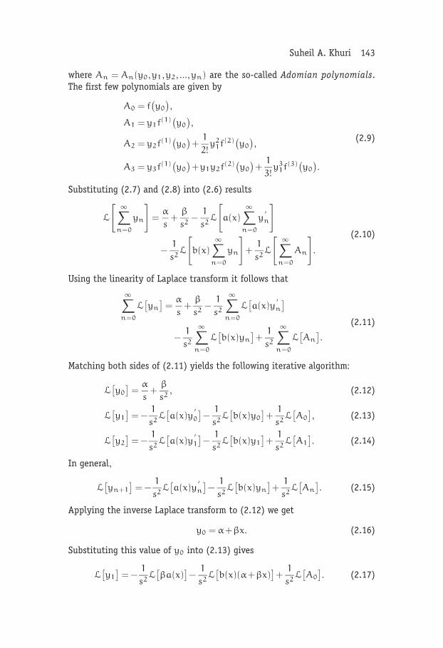
where An = An(y0,y1,y2, ...,yn) are the so-called Adomian polynomials.The first few polynomials are given by
A0 = f(y0
),
A1 = y1f(1)(y0
),
A2 = y2f(1)(y0
)+
1
2!y2
1f(2)(y0
),
A3 = y3f(1)(y0
)+y1y2f(2)
(y0
)+
1
3!y3
1f(3)(y0
).
(2.9)
Substituting (2.7) and (2.8) into (2.6) results
L
[ ∞∑n=0
yn
]=
α
s+
β
s2−
1
s2L
[a(x)
∞∑n=0
y′n
]
−1
s2L
[b(x)
∞∑n=0
yn
]+
1
s2L
[ ∞∑n=0
An
].
(2.10)
Using the linearity of Laplace transform it follows that
∞∑n=0
L[yn
]=
α
s+
β
s2−
1
s2
∞∑n=0
L[a(x)y
′n
]
−1
s2
∞∑n=0
L[b(x)yn
]+
1
s2
∞∑n=0
L[An
].
(2.11)
Matching both sides of (2.11) yields the following iterative algorithm:
L[y0
]=
α
s+
β
s2, (2.12)
L[y1
]= −
1
s2L
[a(x)y
′0
]−
1
s2L
[b(x)y0
]+
1
s2L
[A0
], (2.13)
L[y2
]= −
1
s2L
[a(x)y
′1
]−
1
s2L
[b(x)y1
]+
1
s2L
[A1
]. (2.14)
In general,
L[yn+1
]= −
1
s2L
[a(x)y
′n
]−
1
s2L
[b(x)yn
]+
1
s2L
[An
]. (2.15)
Applying the inverse Laplace transform to (2.12) we get
y0 = α+βx. (2.16)
Substituting this value of y0 into (2.13) gives
L[y1
]= −
1
s2L
[βa(x)
]−
1
s2L
[b(x)(α+βx)
]+
1
s2L
[A0
]. (2.17)
144 Laplace decomposition algorithm
Evaluating the Laplace transform of the quantities on the right-hand sideof (2.17) then applying the inverse Laplace transform, we obtain the valueof y1. The other terms y2,y3, . . . can be obtained recursively in a similarfashion using (2.15).
3. Numerical examples
The Laplace transform decomposition algorithm, described in Section 2, isapplied to some special cases of the class of nonlinear initial-value problemsgiven in (2.1) and (2.2).
Example 3.1. Consider the nonlinear problem
y ′′+(1−x)y ′−y = 2y3, (3.1)
y(0) = 1, y ′(0) = 1, (3.2)
whose closed form solution is
y =1
1−x. (3.3)
Taking Laplace transform of both sides of (3.1) gives
s2L[y]−y(0)s−y ′(0) = −L[(1−x)y ′]+L[y]+2L
[y3
]. (3.4)
The initial conditions (3.2) imply
s2L[y] = s+1−L[(1−x)y ′]+L[y]+2L
[y3
](3.5)
or
L[y] =1
s+
1
s2−
1
s2L
[(1−x)y ′]+
1
s2L[y]+
2
s2L
[y3
]. (3.6)
Following the technique, if we assume an infinite series solution of the form(2.7) we obtain
L
[ ∞∑n=0
yn
]=
1
s+
1
s2−
1
s2L
[(1−x)
∞∑n=0
y′n
]
+1
s2L
[ ∞∑n=0
yn
]+
2
s2L
[ ∞∑n=0
An
],
(3.7)
where the nonlinear operator f(y) = y3 is decomposed as in (2.8) in termsof the Adomian polynomials. From (2.9) the first few Adomian polynomials
Suheil A. Khuri 145
for f(y) = y3 are given by
A0 = y30,
A1 = 3y20y1,
A2 = 3y20y2 +3y0y2
1,
A3 = 3y20y3 +6y0y1y2 +y1
3
. . .
(3.8)
Upon using the linearity of Laplace transform then matching both sides of(3.7), results in the iterative scheme
L[y0
]=
1
s+
1
s2, (3.9)
L[y1
]= −
1
s2L
[(1−x)y
′0
]+
1
s2L
[y0
]+
2
s2L
[A0
], (3.10)
L[y2
]= −
1
s2L
[(1−x)y
′1
]+
1
s2L
[y1
]+
2
s2L
[A1
]. (3.11)
In general,
L[yn+1
]= −
1
s2L
[(1−x)y
′n
]+
1
s2L
[yn
]+
2
s2L
[An
]. (3.12)
Operating with Laplace inverse on both sides of (3.9) gives
y0 = 1+x. (3.13)
Substituting this value of y0 and that of A0 = y30 given in (3.8) into (3.10),
we get
L[y1
]=
1
s2L[2x]+
1
s2L
[(1+x)3
](3.14)
so
L[y1
]=
2
s4+
2
s2
[1
s+
3
s2+
6
s3+
6
s4
]=
2
s3+
8
s4+
12
s5+
12
s6. (3.15)
The inverse Laplace transform applied to (3.15) yields
y1 = x2 +4
3x3 +
1
2x4 +
1
10x5. (3.16)
Substituting (3.16) into (3.11) and using the value of A1 given in (3.8)implies
Simplifying the right-hand side of (3.17) then applying the inverse Laplacetransform, we obtain
y2 = −1
3x3 +
5
12x4 +
7
6x5 +
9
10x6 +
38
105x7 +
3
40x8 +
1
120x9. (3.18)
Higher iterates can be easily obtained using the computer algebra systemMaple. For example,
y3 =1
12x4 −
1
4x5 +
1
40x6 +
4
5x7 +
25
24x8
+361
540x9 +
3233
12600x10 +
29
462x11 +
11
1200x12 +
11
15600x13,
(3.19)
y4 = −1
60x5 +
13
180x6 −
41
280x7 −
1213
6720x8
+7
18x9 +
9991
10800x10 +
14603
16632x11 +
832991
1663200x12
+2066429
10810800x13+
20101
400400x14+
8101
900900x15+
211
208000x16+
211
3536000x17.
(3.20)
Therefore, the approximate solution is
y = y0 +y1 +y2 +y3 +y4 + · · ·
= 1+x+x2 +x3 +x4 +x5 +359
360x6 +
853
840x7 +
2097
2240x8
+1151
1080x9 +
17867
15120x10 +
15647
16632x11 +
848237
1663200x12 +
518513
2702700x13
+20101
400400x14 +
8101
900900x15 +
211
208000x16 +
211
3536000x17 + · · · .
(3.21)
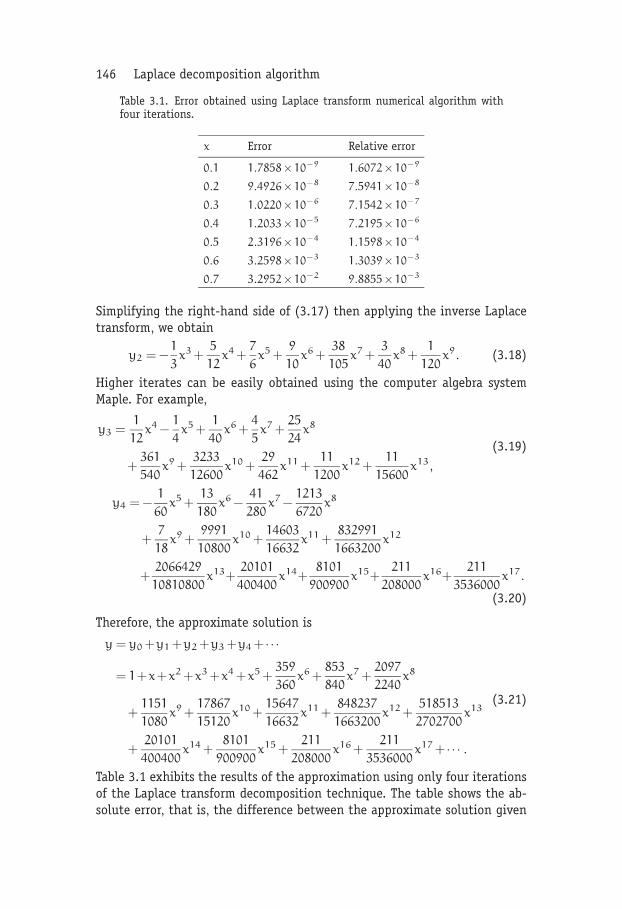
Table 3.1 exhibits the results of the approximation using only four iterationsof the Laplace transform decomposition technique. The table shows the ab-solute error, that is, the difference between the approximate solution given
Suheil A. Khuri 147
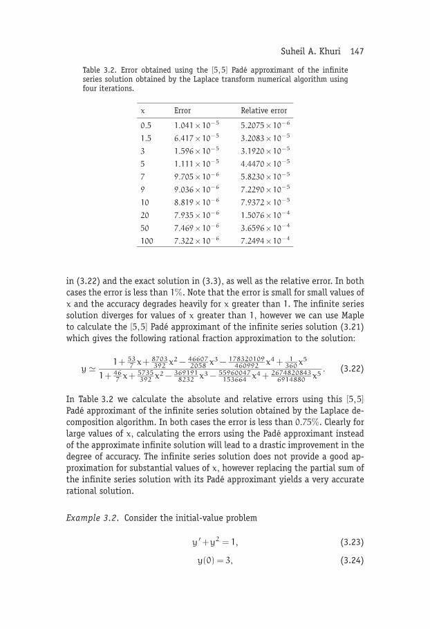
Table 3.2. Error obtained using the [5,5] Pade approximant of the infiniteseries solution obtained by the Laplace transform numerical algorithm usingfour iterations.
x Error Relative error
0.5 1.041×10⁻⁵ 5.2075×10⁻⁶
1.5 6.417×10⁻⁵ 3.2083×10⁻⁵
3 1.596×10⁻⁵ 3.1920×10⁻⁵
5 1.111×10⁻⁵ 4.4470×10⁻⁵
7 9.705×10⁻⁶ 5.8230×10⁻⁵
9 9.036×10⁻⁶ 7.2290×10⁻⁵
10 8.819×10⁻⁶ 7.9372×10⁻⁵
20 7.935×10⁻⁶ 1.5076×10⁻⁴
50 7.469×10⁻⁶ 3.6596×10⁻⁴
100 7.322×10⁻⁶ 7.2494×10⁻⁴
in (3.22) and the exact solution in (3.3), as well as the relative error. In bothcases the error is less than 1%. Note that the error is small for small values ofx and the accuracy degrades heavily for x greater than 1. The infinite seriessolution diverges for values of x greater than 1, however we can use Mapleto calculate the [5,5] Pade approximant of the infinite series solution (3.21)which gives the following rational fraction approximation to the solution:
y � 1+ 537 x+ 8703
392 x2 − 466072058 x3 − 178320109
460992 x4 + 1360x5
1+ 467 x+ 5735
392 x2 − 3691918232 x3 − 55960047
153664 x4 + 26748208436914880 x5
. (3.22)
In Table 3.2 we calculate the absolute and relative errors using this [5,5]
Pade approximant of the infinite series solution obtained by the Laplace de-composition algorithm. In both cases the error is less than 0.75%. Clearly forlarge values of x, calculating the errors using the Pade approximant insteadof the approximate infinite solution will lead to a drastic improvement in thedegree of accuracy. The infinite series solution does not provide a good ap-proximation for substantial values of x, however replacing the partial sum ofthe infinite series solution with its Pade approximant yields a very accuraterational solution.
Example 3.2. Consider the initial-value problem
y ′+y2 = 1, (3.23)
y(0) = 3, (3.24)
148 Laplace decomposition algorithm
whose closed form solution is
y = −1+2
1− .5e−2x. (3.25)
First, we apply Laplace transform to both sides of (3.23),
sL[y]−y(0)+L[y2
]=
1
s. (3.26)
The initial condition (3.24) gives
L[y] =3
s+
1
s2−
1
sL
[y2
]. (3.27)
Assuming an infinite series solution of the form (2.7), we have
L
[ ∞∑n=0
yn
]=
3
s+
1
s2−
1
sL
[ ∞∑n=0
An
], (3.28)
where the nonlinear operator f(y) = y2 is decomposed as in (2.8) in termsof the Adomian polynomials. From (2.9) the first few Adomian polynomialsare
A0 = y20,
A1 = 2y0y1,
A2 = 2y0y2 +y21,
A3 = 2y0y3 +2y1y2
. . .
(3.29)
Following the Laplace transform decomposition method, if we match bothsides of (3.27) we obtain the iterative scheme
L[y0
]=
3
s+
1
s2, (3.30)
L[y1
]= −
1
sL
[A0
], (3.31)
L[y2
]= −
1
sL
[A1
], (3.32)
and the general iterative step is
L[yn+1
]= −
1
sL
[An
]. (3.33)
The inverse Laplace transform applied to (3.30) results
y0 = 3+x. (3.34)
Suheil A. Khuri 149
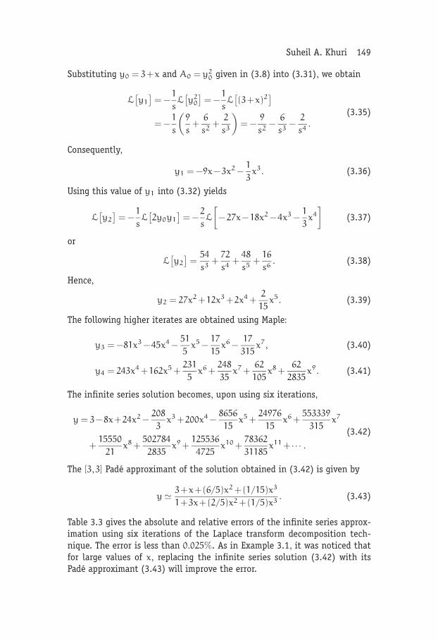
Substituting y0 = 3+x and A0 = y20 given in (3.8) into (3.31), we obtain
L[y1
]= −
1
sL
[y2
0
]= −
1
sL
[(3+x)2
]= −
1
s
(9
s+
6
s2+
2
s3
)= −
9
s2−
6
s3−
2
s4.
(3.35)
Consequently,
y1 = −9x−3x2 −1
3x3. (3.36)
Using this value of y1 into (3.32) yields
L[y2
]= −
1
sL
[2y0y1
]= −
2
sL
[−27x−18x2 −4x3 −
1
3x4
](3.37)
or
L[y2
]=
54
s3+
72
s4+
48
s5+
16
s6. (3.38)
Hence,
y2 = 27x2 +12x3 +2x4 +2
15x5. (3.39)
The following higher iterates are obtained using Maple:
y3 = −81x3 −45x4 −51
5x5 −
17
15x6 −
17
315x7, (3.40)
y4 = 243x4 +162x5 +231
5x6 +
248
35x7 +
62
105x8 +
62
2835x9. (3.41)
The infinite series solution becomes, upon using six iterations,
y = 3−8x+24x2 −208
3x3 +200x4 −
8656
15x5 +
24976
15x6 +
553339
315x7
+15550
21x8 +
502784
2835x9 +
125536
4725x10 +
78362
31185x11 + · · · .
(3.42)
The [3,3] Pade approximant of the solution obtained in (3.42) is given by
y � 3+x+(6/5)x2 +(1/15)x3
1+3x+(2/5)x2 +(1/5)x3. (3.43)
Table 3.3 gives the absolute and relative errors of the infinite series approx-imation using six iterations of the Laplace transform decomposition tech-nique. The error is less than 0.025%. As in Example 3.1, it was noticed thatfor large values of x, replacing the infinite series solution (3.42) with itsPade approximant (3.43) will improve the error.
150 Laplace decomposition algorithm
Table 3.3. Error obtained upon using six iterations of the Laplace transformdecomposition algorithm.
x Error Relative error
0.1 2.9849×10⁻¹⁰ 1.2509×10⁻¹⁰
0.2 2.4803×10⁻⁸ 1.2351×10⁻⁸
0.3 2.9356×10⁻⁷ 1.6714×10⁻⁷
0.4 1.5941×10⁻⁶ 1.0092×10⁻⁶
0.5 5.6963×10⁻⁶ 3.9263×10⁻⁶
0.6 1.5688×10⁻⁵ 1.1581×10⁻⁵
0.7 3.6180×10⁻⁵ 2.8237×10⁻⁵
0.8 7.3380×10⁻⁵ 5.9923×10⁻⁵
0.9 1.3503×10⁻⁴ 1.1441×10⁻⁴
1.0 2.3023×10⁻⁴ 2.0105×10⁻⁴
Example 3.3. Consider the following nonlinear problem:
y ′ = 4y−y3, (3.44)
y(0) = 0.5. (3.45)
The exact solution is
y = 2
(e8x
e8x +15
)1/2
. (3.46)
Operating with Laplace transform on both sides of (3.44) results
sL[y]−y(0) = 4L[y]−L[y3
]. (3.47)
Using the initial condition (3.45) then simplifying the resulting equation in(3.47), we obtain
L[y] =0.5
s+
4
sL[y]−
1
sL[y3
]. (3.48)
Assuming an infinite series solution as in (2.7) we have
L
[ ∞∑n=0
yn
]=
0.5
s+
4
sL
[ ∞∑n=0
yn
]−
1
sL
[ ∞∑n=0
An
], (3.49)
where the nonlinear operator f(y) = y3 is decomposed as in (2.8) in termsof the Adomian polynomials, which for this case the first few are given in(3.8). Matching both sides of (3.49), the components of y can be defined
Suheil A. Khuri 151
as follows:
L[y0
]=
0.5
s, (3.50)
L[y1
]=
4
sL
[y0
]−
1
sL
[A0
], (3.51)
L[y2
]=
4
sL
[y1
]−
1
sL
[A1
](3.52)
and the general term is
L[yn+1
]=
4
sL
[yn
]−
1
sL
[An
]. (3.53)
The terms yn can be obtained in a recursive manner. Taking the inverseLaplace transform of (3.50) gives
y0 = 0.5. (3.54)
Substituting this value of y0 into (3.51), and using that A0 = y30 from (3.8),
we obtain
L[y1
]=
2
s2−
1
sL
[(0.5)3
]=
2
s2−
1
8s2. (3.55)
It follows that
y1 = 1.875x. (3.56)
Using this value of y1 into (3.52) gives
L[y2
]=
4
sL[1.875x]−
1
sL
[3y2
0y1
]. (3.57)
Consequently
y2 = 3.046875x2. (3.58)
The next higher iterates are obtained using Maple,
y3 = 1.54296875x3,
y4 = −4.678955079x4.(3.59)
The series solution is therefore
y = 0.5+1.875x+3.046875x2 +1.54296875x3
−4.678955079x4 −13.98919678x5 + · · · . (3.60)
The [4,4] Pade approximant of this approximate solution is
y � 0.5+2.940330021x+9.262070767x2 +13.01811008x3 +9.597056446x4
Table 3.4. Error obtained using four iterations of the numerical algorithm.
x Error Relative error
0.05 2.5873×10⁻⁷ 4.3013×10⁻⁷
0.10 1.5733×10⁻⁵ 2.1885×10⁻⁵
0.15 1.6370×10⁻⁴ 1.9226×10⁻⁴
0.20 7.9299×10⁻⁴ 7.9581×10⁻⁴
0.25 2.3856×10⁻³ 2.0763×10⁻³
0.30 4.8087×10⁻³ 3.6942×10⁻³
0.35 5.6245×10⁻³ 3.8888×10⁻³
0.40 2.3004×10⁻³ 1.4601×10⁻³
Table 3.4 shows that the absolute and relative errors of the approximation(3.61), using four iterations of the numerical technique, is less than 2%.Again, as in the previous examples, the Pade approximant (3.61) of the so-lution (3.60) yields a better approximation of the exact solution for largervalues of x.
Example 3.4. In this last example, the method is illustrated by consideringthe damped Duffing’s equation
y ′′+ky ′ = −y3, (3.62)
y(0) = α, y ′(0) = β, (3.63)
where k is a positive constant. Applying Laplace transform to both sides of(3.62) we obtain
s2L[y]−y(0)s−y ′(0)+k(sL[y]−y(0)
)= −L
[y3
]. (3.64)
Simplifying this equation and using the initial conditions (3.63) yields(s2 +ks
)L[y] = α(s+k)+β−L
[y3
](3.65)
or
L[y] = αs+k
s2 +ks+
β
s2 +ks−
1
s2 +ksL
[y3
]. (3.66)
Assuming an infinite series solution of the form (2.7) we get
L
[ ∞∑n=0
yn
]= α
s+k
s2 +ks+
β
s2 +ks−
1
s2 +ksL
[ ∞∑n=0
An
], (3.67)
where the nonlinear operator f(y) = y3 is decomposed in terms of theAdomian polynomials which for this case are given in (3.8). Upon using
Suheil A. Khuri 153
the linearity of Laplace transform then matching both sides of (3.67),results in the iterative algorithm
L[y0
]= α
s+k
s2 +ks+
β
s2 +ks, (3.68)
L[y1
]= −
1
s2 +ksL
[A0
], (3.69)
L[y2
]= −
1
s2 +ksL
[A1
]. (3.70)
In general,
L[yn+1
]= −
1
s2 +ksL
[An
]. (3.71)
Consider the case where α = β = k = 1. Operating with Laplace inverse onboth sides of (3.68) gives
y0 = 2−e−x. (3.72)
Substituting this value of y0 and that of A0 = y30 given in (3.8) into (3.69),
we obtain
L[y1
]= −
1
s2 +ksL
[y3
0
]= −
1
s2 +ksL
[(2−e−x
)3](3.73)
so
L[y1
]=
8/s−12/(s+1)+6/(s+2)−1/(3+s)
s2 +s. (3.74)
The inverse Laplace transform applied to (3.74) yields
y1 = −8x+52
3−12xe−x −
29
2e−x −3e−2x +
1
6e−3x. (3.75)
Substituting the value of A1 given in (3.8) into (3.70) implies
L[y2
]= −
1
s2 +ksL
[3y2
0y1
]. (3.76)
Substituting the values of y0 and y1 given in (3.72) and (3.75) into (3.76)then applying the inverse Laplace transform, we obtain
y2 = 48x2 −304x+37049
60−
(24x2 +430x+
10543
24
)e−x
−(60x+185
)e−2x +
(6x+
71
12
)e−3x +
11
12e−4x −
1
40e−5x.
(3.77)
154 Laplace decomposition algorithm
Table 3.5. Error that results from comparing the solution derived by theLaplace transform numerical algorithm with four iterations, and the numericalsolution obtained using Maple.
x Error Relative error
0.1 1.6482×10⁻¹⁰ 1.5123×10⁻¹⁰
0.2 3.7401×10⁻¹⁰ 3.2275×10⁻¹⁰
0.3 3.6991×10⁻⁸ 3.0661×10⁻⁸
0.4 7.8776×10⁻⁷ 6.3895×10⁻⁷
0.5 8.5726×10⁻⁶ 6.9187×10⁻⁶
0.6 6.0690×10⁻⁵ 4.9478×10⁻⁵
0.7 3.1769×10⁻⁴ 2.6522×10⁻⁴
0.8 1.3281×10⁻³ 1.1494×10⁻³
0.9 4.6628×10⁻³ 4.2292×10⁻³
1.0 1.4236×10⁻² 1.3664×10⁻²
In a similar fashion, higher iterates are obtained using Maple. For example,
y3 = −320x3 +3616x2 −246667
15x+
184833613
6300
+
(32x3 −796x2 −
545719
30x−
71534779
3600
)e−x
+
(84x2 +
1055
3x+
9103
144
)e−3x −
(3
2x+
29
400
)e−5x
−
(360x2 +4308x+
385069
40
)e−2x +
(121
3x+
863
9
)e−4x
+19
5040e−7x −
373
1800e−6x.
(3.78)
Therefore, the approximate solution is
y = y0 +y1 +y2 +y3 + · · ·
= −251347
15x−320x3 −
(392589
40+4368x+360x2
)e−2x
−
(39
400+
3
2x
)e−5x +
(84x2 +
1073
3x+
9979
144
)e−3x
−
(73172029
3600+32x3 +
558979
30x+820x2
)e−x +3664x2
+
(121
3x+
3485
36
)e−4x −
373
1800e−6x +
19
5040e−7x +
94422779
3150+ · · · .
(3.79)
Suheil A. Khuri 155
Table 3.5 shows the absolute and relative errors that result from compar-ing the approximate solution obtained from the Laplace transform decom-position algorithm using four iterations, and the numerical solution of thedamped Duffing’s equation evaluated using Maple solve commands. The erroris less than 0.001%. In all the previous four examples, it was observed thatincreasing the number of iterates will improve the accuracy of the solution.
References
[1] G. Adomian, A review of the decomposition method and some recent resultsfor nonlinear equations, Comput. Math. Appl. 21 (1991), no. 5, 101–127.MR 92h:00002b. Zbl 0732.35003.
[2] , Solving Frontier Problems of Physics: The Decomposition Method,
Journal of Applied Mathematics and Decision Sciences
Special Issue on
Decision Support for Intermodal Transport
Call for Papers
Intermodal transport refers to the movement of goods ina single loading unit which uses successive various modesof transport (road, rail, water) without handling the goodsduring mode transfers. Intermodal transport has becomean important policy issue, mainly because it is consideredto be one of the means to lower the congestion caused bysingle-mode road transport and to be more environmentallyfriendly than the single-mode road transport. Both consider-ations have been followed by an increase in attention towardintermodal freight transportation research.
Various intermodal freight transport decision problemsare in demand of mathematical models of supporting them.As the intermodal transport system is more complex than asingle-mode system, this fact offers interesting and challeng-ing opportunities to modelers in applied mathematics. Thisspecial issue aims to fill in some gaps in the research agendaof decision-making in intermodal transport.
The mathematical models may be of the optimization typeor of the evaluation type to gain an insight in intermodaloperations. The mathematical models aim to support deci-sions on the strategic, tactical, and operational levels. Thedecision-makers belong to the various players in the inter-modal transport world, namely, drayage operators, terminaloperators, network operators, or intermodal operators.
Topics of relevance to this type of decision-making both intime horizon as in terms of operators are:
• Intermodal terminal design• Infrastructure network configuration• Location of terminals• Cooperation between drayage companies• Allocation of shippers/receivers to a terminal• Pricing strategies• Capacity levels of equipment and labour• Operational routines and lay-out structure• Redistribution of load units, railcars, barges, and so
forth• Scheduling of trips or jobs• Allocation of capacity to jobs• Loading orders• Selection of routing and service
Before submission authors should carefully read over thejournal’s Author Guidelines, which are located at http://www.hindawi.com/journals/jamds/guidelines.html. Prospectiveauthors should submit an electronic copy of their completemanuscript through the journal Manuscript Tracking Sys-tem at http://mts.hindawi.com/, according to the followingtimetable:
Manuscript Due June 1, 2009
First Round of Reviews September 1, 2009
Publication Date December 1, 2009
Lead Guest Editor
Gerrit K. Janssens, Transportation Research Institute(IMOB), Hasselt University, Agoralaan, Building D, 3590Diepenbeek (Hasselt), Belgium; [email protected]
Guest Editor
Cathy Macharis, Department of Mathematics, OperationalResearch, Statistics and Information for Systems (MOSI),Transport and Logistics Research Group, ManagementSchool, Vrije Universiteit Brussel, Pleinlaan 2, 1050 Brussel,Belgium; [email protected]