1

A Light Signalling Approach to Node Grouping forMassive MIMO IoT Networks

Emma Fitzgerald, Michał Pioro, Harsh Tataria, Gilles Callebaut, Sara Gunnarsson and Liesbet Van der Perre

Abstract—Massive MIMO is a promising technology to connectvery large numbers of energy constrained nodes, as it offers bothextensive spatial multiplexing and large array gain. A challengeresides in partitioning the many nodes in groups that cancommunicate simultaneously such that the mutual interferenceis minimized. We here propose node partitioning strategies thatdo not require full channel state information, but rather arebased on nodes’ respective directional channel properties. In ourconsidered scenarios, these typically have a time constant that isfar larger than the coherence time of the channel. We developedboth an optimal and an approximation algorithm to partitionusers based on directional channel properties, and evaluatedthem numerically. Our results show that both algorithms, despiteusing only these directional channel properties, achieve similarperformance in terms of the minimum signal-to-interference-plus-noise ratio for any user, compared with a reference methodusing full channel knowledge. In particular, we demonstratethat grouping nodes with related directional properties is to beavoided. We hence realise a simple partitioning method requiringminimal information to be collected from the nodes, and wherethis information typically remains stable over a long term, thuspromoting their autonomy and energy efficiency.

Index Terms—massive MIMO; IoT; user grouping; energyefficiency

I. INTRODUCTION

It is clear by now that massive multiple-input multiple-output (MIMO) is a key concept for enhancing the capacity inbroadband wireless networks. The use of many electronicallysteerable service antennas at the base station facilitates aggres-sive spatial multiplexing to tens of user equipment nodes. Thisenables a substantial increase in the link reliability and spectralefficiency experienced by a particular node. In situations wherethe massive MIMO array is required to simultaneously servea very large number of nodes, there arises the challenge ofgrouping and scheduling these nodes for transmission. This is

E. Fitzgerald, H. Tataria, S. Gunnarsson, and L. Van der Perre arewith the Department of Electrical and Information Technology, LundUniversity, SE-221 Lund, Sweden (e-mail: {emma.fitzgerald, harsh.tataria,sara.gunnarson}@eit.lth.se).

M. Pioro is with the Institute of Telecommunication, Warsaw Univer-sity of Technology, Nowowiejska 15/19, 00-665 Warsaw, Poland (e-mail:m.pioro@tele.pw.edu.pl).

G. Callebaut, S. Gunnarsson and L. Van der Perre are withthe Department of Electrical Engineering, KU Leuven, Gebroedersde Smetstraat 1, 9000 Ghent, Belgium (e-mail: {gilles.callebaut, lies-bet.vanderperre}@kuleuven.be).

The work of E. Fitzgerald and M. Pioro was supported by the NationalScience Centre, Poland, under grant no. 2017/25/B/ST7/02313: “Packet rout-ing and transmission scheduling optimization in multi-hop wireless networkswith multicast traffic”. The work of E. Fitzgerald was also partially supportedby the Celtic-Next project 5G PERFECTA, the SSF project SEC4FACTORYunder grant no. SSF RIT17-0032, as well as the strategic research area ELLIIT.The work of H. Tataria was partly supported by Ericsson AB, Sweden.

particularly important for the massive machine-type commu-nication (mMTC) use case, where extremely large numbersof nodes may be present within the same geographical areaserved by the base station [1].

In this paper we propose a node grouping method based ondirectional properties of the nodes’ channels that are stableover long periods of time and so do not need to be updatedat the rate of the coherence time of the channel. This reducessignalling overhead and makes our method suitable for use asa precursor to node scheduling for energy constrained Internetof Things (IoT) nodes with infrequent transmissions. Weformulate this as an optimisation problem using mixed-integerprogramming. We then develop an efficient approximationalgorithm to solve this problem much faster than is possible forthe optimisation. Our results show that both our optimisationand approximation provide superior performance in termsof minimum signal-to-interference-plus-noise ratio (SINR) incomparison to a reference method based on grouping nodesby their instantaneous signal strength, that is, received powertaking into account both small and large-scale fading. Thelatter requires full small scale channel state information (CSI)that is in practice not possible to collect a-priori.

The contributions of this paper are:

• A node partitioning method for massive MIMO systemsbased on simple directional characteristics of the nodes’channels, namely dominant direction and angular spec-trum spread, allowing for stable partitioning over a longtime period with minimal signalling by the node devices.The partitioning is complete in the sense that every nodebelongs to a group, so that all nodes are served.

• A formulation of the node partitioning problem usingdirectional channel characteristics as an optimisationproblem using mixed integer programming.

• An efficient approximation algorithm to solve the prob-lem that runs in O(nlogn) time.

• A numerical evaluation of the optimisation problem andapproximation algorithm using network examples gen-erated from a suitable channel model, showing similarperformance for our partitioning method compared tousing full channel information.

The rest of this paper is organised as follows. Section IIintroduces and motivates our node grouping approach. Sec-tion III then discusses related work on node partitioningand scheduling in massive MIMO systems. Next, Section IVdetails our problem setting and defines the node partitioningproblem. The partitioning problem is then formulated as amixed-integer optimisation problem in Section V, and our

arX

iv:2

005.

0504

8v1

[cs

.NI]

11

May

202

0

2

approximation algorithm to solve this problem more efficientlyis given in Section VI. We present our numerical evaluationof the optimisation problem and approximation algorithm inSection VII. Finally, in Section VIII, we conclude this paperand discuss future work.

II. MOTIVATION

Many IoT devices are battery-powered, making energy effi-ciency a critical performance criterion. Such devices typicallyspend a large proportion of their time in the so-called sleepmode, i.e., in a low-power state to conserve energy, only“waking up” when it is necessary to send or receive data.These devices’ corresponding transmission also often occursinfrequently1. Depending on the device type — often a sensornode — and its configuration with the network, there is a largevariation in the timescale when transmission and receptionneed to take place, with the absolute timescale varying fromminutes up to tens of days or longer. At such time scales,efficient node grouping and scheduling becomes difficult, sinceinformation about the node traffic and propagation channelscan quickly become outdated, unless additional signalling isintroduced, which in turn requires nodes to wake up andtransmit more often, consuming more energy.

Node grouping consists of partitioning the nodes into groupssuch that each group can be accommodated for simultaneoustransmission in the same coherence block, giving a combi-nation of spatial and time multiplexing. This subsequentlyallows scheduling of node groups rather than individual nodes,thus reducing the complexity of the scheduling problem. Forlow-power IoT devices, this partition should be based onnode properties that are stable over considerable time, sothat schedules based on them can cover a reasonable numberof transmissions. Too frequent scheduling requires a costlysignalling overhead to collect, in advance, the informationneeded to construct the schedule as well as inform the nodesof the result. Scheduling may also have significant costs interms of computation, depending on the scheduling algorithmused.

In addition to being stable over time, node properties usedfor grouping must also be informative for network perfor-mance in order to create schedules that achieve good perfor-mance. Poor performance, for example, in terms of low SINRscan incur an increase of the node’s energy consumption by re-quiring it to use a more robust modulation and coding method.This may lead to longer transmission times, or increasingbit error rates, necessitating retransmissions when packets areunable to be decoded. To this end, interference within thenode groups should be minimized by exploiting characteristicsof propagation channels that remain stable over a long time,ideally at least over some tens of node transmissions, and aslong as possible to allow for long scheduling windows. Thisis the subject of this paper.

One possible candidate for a stable channel property islong-term average signal strength, characterised by the averagereceived power (naturally comprised by the power transmitted

1We recognise that some IoT devices may need to constantly send or receivedata, however here we focus on typical sensors with infrequent transmissions.

Fig. 1. Two node partitioning approaches: “pizza” partitioning (left), in whichnodes are grouped such that the nodes in each group have large differencesin their directions from the base station; and “onion” partitioning, in whichnodes with similar signal strength are grouped together. With line of sight andfree space propagation, shown here, the former is equivalent to dividing thenodes into angular slices, while the latter is equivalent to grouping the nodesinto rings by distance from the base station.

from the node, as well as large-scale fading). This propertycan have a significant impact on the inter-node interferencein massive MIMO, particularly when simple maximum ratiocombining (MRC) is used for precoding [2]. Furthermore,the average received power can be effectively used for nodegrouping and scheduling [3]. Nevertheless, inter-node interfer-ence can also be strongly affected by the directional propertiesof the users’ channels. Indeed measurement campaigns haveshown that propagation energy typically features dominantdirections, and even in reflective environments, real channelresponses are far from “ideal” independent and identicallydistributed Rayleigh fading channels commonly assumed intheory [4]–[6]. This observation suggests that node partitioningthat avoids simultaneously scheduling nodes with propagationenergy coming from similar directions can actually preventinter-node interference to a large extent2. It is these solutionswe investigate in this work. The methods developed in thispaper could also easily be combined with node grouping basedon signal strength, especially in cases where there are a largenumber of nodes and node groups.

We develop a node partitioning method for massive MIMOsystems based on two directional properties of the nodes’channels, namely dominant direction — the angle of arrivalof the strongest channel component — and angular spectrumspread — how widely the channel components are distributedover the possible range of angles of arrival. These propertiesare stable over larger time scales than the full CSI that changesaccording to the channel’s coherence time, easy to collect atthe base station with minimal signalling, and correlate withinter-node interference. We formulate an optimisation problemto find a partition of the nodes into groups that maximizes theminimum angular difference between nodes across multipledifferent groups according to their angular spectrum spreads,

2In terms of the ergodic sum spectral efficiency, naturally there is a price topay to reduce inter-node interference through user grouping. However, giventhe low data rates required by typical IoT applications, energy efficiency is amore important performance metric for this use case than spectral efficiency.

3

as well as devise an approximation algorithm following thesame principle.

This approach is analogous to partitioning the nodes withinthe coverage of a centrally located base station into pizzaslices, such that each slice only contains one node from eachgroup (Fig. 1, left). This can be compared to an onion ringpartitioning approach, where nodes are grouped such thatnodes with similar signal strength are placed in the samegroup. With line of sight and free space propagation, thiswould result in the groups forming concentric shells, similarto the rings of an onion (Fig. 1, right). In more complexchannel environments, especially with shadowing or multipathcomponents, the slices and rings will not have such simplegeometric shapes as shown in the figure and may even consistof multiple disjoint regions. While we focus on the pizzaapproach in this paper, with sufficiently many nodes, the twomethods can be readily combined, by simply composing them,for example dividing the nodes into onion rings and then intopizza slices, or vice versa.

III. RELATED WORK

Thus far, there has been limited work on node partitioningin massive MIMO in the sense we consider in this paper. Thereis a substantial body of work on node selection, starting withmultiuser MIMO (MU-MIMO) systems [7]–[10] even beforethe advent of massive MIMO. However, the goal of thesestudies is to choose some subset of the available nodes to beserved at a given point in time, typically to maximise the sumrate of the system. Although this is often referred to as nodescheduling, it is not true scheduling in that nodes that are notserved are not scheduled to be served in future: the nodes arerather partitioned into those that are served, and those that arenot, with the assumption that as channel conditions change,different nodes will be served over time. We are howeverinterested in node partitioning for the purpose of then creatinga schedule for all node groups to be served over time. As such,multiple groups are created, and all nodes must be includedin at least one group for the partition to be valid. To avoidconfusion, we will therefore reserve the term scheduling tomean arranging service of nodes or node groups over timesuch that all nodes or groups are eventually served, and usethe term selection to mean selecting some subset of nodes forservice at a given point in time.

Furthermore, our objective is not to maximise the sum rateof the system. In many IoT use cases, high throughput is notneeded. Rather, the aim is often to serve all node demandswith minimal energy usage. Here, the rate provided to anindividual node does have some relation to this goal, since ahigh achievable data rate can be used rather to reduce bit errorsand thus increase reliability, instead of maximizing throughput.Fewer bit errors mean fewer retransmissions, and thus energysaved. Beyond a certain point, however, nodes do not benefitfrom a higher SINR as they only have a small amount of data,for example sensor or control data, to transmit or receive. Assuch, we want to find a node grouping that maximizes theminimum SINR of any node, rather than maximizing the sumrate.

Despite these differences, work on node selection is relevantto our work, since a full node grouping can be regarded asan extension to the binary partitioning of nodes into thosethat are served and those that are not, and can use similarapproaches. We will first discuss the extensive body of workon node selection, and then consider the more limited existingwork on scheduling and random access in massive MIMOsystems.

A. Node Selection for Massive MIMO

When selecting nodes for transmission, many approachesrely on full CSI, such as [11]–[14]. This is however notsuitable to our use case since this would require all nodesto first wake up from sleep, and then transmit a pilot signal inorder for the base station to gather the CSI. For low power IoTdevices, such an approach would consume too much energy tobe viable, and does not allow the schedule to be set in advanceto provide a defined sleep opportunity and wake up time.

There is however a body of work that performs nodegrouping based on reduced channel information, which isusually more stable over time. This is often done in the contextof two-stage beamforming, where pre-beamforming groups arefirst formed using coarse channel information, and then fullprecoding takes place after collecting full CSI for a subset ofnodes. Some examples of reduced information that can be usedfor this purpose are channel quality indicators [15], directionalinformation collected from downlink probing [16], and thecovariance matrices of node channels [15], [17], [18], whichcan be determined over time by recording statistical channelinformation. Of particular interest to us are spatial clusteringmethods [19], sometimes also used in combination with theabove techniques.

One approach that has similarities to ours is that of jointspatial division and multiplexing (JSDM) [18], [20]. In thismethod, artificial covariance matrices are constructed basedon a set of angles of arrival and angular spreads. Nodes arethen clustered into sectors based on the similarity of theirchannels, for example by computing the chordal distancesof the eigenspaces of nodes’ channel covariance matricesto those of the constructed ones. One key result, provedin [20], is that for a uniformly spaced linear array, JSDMapproaches optimality, in terms of maximizing the sum rate,as the number of antennas grows. This is because the nodechannels, when grouped according to their angles of arrivaland angular spreads, form near-orthogonal subspaces. Whilethe objective of JSDM is different to that of our work, thisdemonstrates the value of node grouping based on directionalcharacteristics, which we also use in our approach.

All of the above work is focused on node selection, withthe goal of maximizing the sum rate of the system at aspecific point in time. Once node grouping is performed, itis then immediately used to collect full CSI from a subset ofnodes and then serve them. We, however, seek to find a nodegrouping that can be used over a longer period of time toschedule service of low power IoT devices, and the above workis not suitable for such a case for a number of reasons. Firstly,we do not wish to select a subset of nodes for service, but

4

rather serve all nodes, although at different times according towhich group they belong to. An optimal partitioning of nodeswhere only a subset will be served may be quite differentto one where all nodes must be served. In our scenario,nodes with a low signal-to-noise ratio (SNR) or that interferesignificantly with other nodes cannot be simply dropped toimprove overall performance, but must be accommodated insome group.

A few existing works on node grouping do consider otherobjectives. [12] groups nodes into multicast groups accordingto their interests, with the objective of maximizing minimumthroughput. However, here, full CSI is used, which is notfeasible for low power IoT. [11] focuses on IoT, primarilyconsidering the aspect of serving a large number of nodes,rather than low energy usage, since again full CSI is usedand the objective is maximal sum rate. One interesting aspectof this work is that node groups may overlap, such that eachnode can be served by more than one group, helping to ensurefull coverage. In our work, we use disjoint node groups, butthis could be extended to overlapping groups in future, forexample for nodes that have a higher traffic demand or poorSINR. [15] performs node selection as in the other work above,however this is done in combination with fair scheduling, toavoid starvation of nodes that would otherwise be repeatedlynot selected. This still does not provide a predictable schedulethat would allow a node to sleep until its appointed servicetime, since nodes are still selected dynamically in each timeslot.

B. Node Scheduling and Random Access for Massive MIMO

There is also some, albeit limited, existing work on nodescheduling for massive MIMO. Because massive MIMO sys-tems serve multiple nodes simultaneously, such schedulinginherently requires creating node groups, although the groupsdo not necessarily need to be disjoint. In [3], joint nodescheduling and transmission power control is performed fornodes with heterogeneous traffic demands. However, here,information about the traffic queues at each node is required,which increases the signalling needed and thus the energy cost.[21] examines fair scheduling in massive MIMO systems, butprovides an analysis of the achievable fair rate, rather than asolution for actually performing scheduling.

Some work has also investigated random access for IoTdevices in massive MIMO systems [22]–[26]. Random accessis a promising solution for many IoT scenarios, especiallyif it is grant free, since signalling overhead is reduced, anddevices can choose when to wake up and transmit. However, incases where there is a high level of contention, random accesscan lead to collisions, which induce retransmissions and costenergy while further increasing the contention for the channel.Scheduled access also provides more predictable performance,which can be important for some applications. Nevertheless,random access protocols could be combined with our nodegrouping method, by allowing entire node groups to wake upduring a limited period, in which they would be served throughrandom access. Such an approach reduces contention while atthe same time allowing devices in other groups to sleep until

it is their turn. Alternatively, our node grouping could be usedas the precursor to any scheduling algorithm, such as roundrobin or fair scheduling, both to schedule entire groups, andnodes within each group. In all these cases, node groupingsimplifies network control, since devices can be orchestratedat group level instead of addressing each individual device,and provides for predictable and extended sleep opportunitiesuntil it is time for a given group to be served.

IV. SCENARIO AND PROBLEM DEFINITION

We consider a single-cell network with the base stationequipped with a large, central antenna array, and a number ofsingle-antenna nodes. We particularly focus on IoT devices,such as sensors, that require low energy usage. We hereconsider static node devices, and they could be placed indifferent environments (urban, indoors, rural, etc.). Althoughthe devices themselves do not move, there may nonethelessbe some movement in the environment, for example peoplewalking around.

We here give a brief overview of massive MIMO trans-mission underlying to our work. For more details, the inter-ested reader is referred to [2]. In a massive MIMO system,transmission is established according to the coherence blocksof the channel. A coherence block is a time by frequencyregion in which the channel is constant, to within some smallmargin of error. Within each coherence block, nodes transmitpilot signals in order for the base station to determine the CSIand thus allow data transmission and reception. We considera time-division duplex massive MIMO system, relying onchannel reciprocity within each coherence block, and hencenot requiring downlink pilots.

In each coherence block, a number of nodes are servedsimultaneously, for either uplink or downlink transmission,or both. The number of nodes that may be served in eachcoherence block is limited by either the number of availablepilot signals — since each node must be allocated a pilot inorder to transmit or receive in the block — or by the inter-nodeinterference, or both. The interference between nodes dependson both the combination of their channels and the precodingscheme used. In this work, we focus on MRC as precoding.

In scenarios where the number of nodes exceeds the numberthat can be served simultaneously in one coherence block,node grouping becomes necessary, such that each group canbe accommodated in a single coherence block. After grouping,node groups can then be scheduled by assigning coherenceblocks to them such that the traffic demands of all nodesin the group are satisfied. In this paper, we do not considerscheduling, but rather focus on the node partitioning problem.

In this work, we perform node grouping based on twodirectional characteristics of the node channels. The first isthe dominant propagation direction, that is, the direction fromwhich the dominant component of a given node channel arrivesat the base station. The second characteristic we use is theangular spectrum spread: how much the power of the nodechannel, as received by the base station, is spread over theangular domain. A low angular spectrum spread thus impliesa channel where the power is largely focused in the dominant

5

−90 −60 −30 0 30 60 90

0

0.2

0.4

0.6

0.8

1.0

Angle (◦)

Nor

mal

ised

Pow

erHigh angular spectrum spreadLow angular spectrum spread

Fig. 2. Two example channels with a high and low angular spectrum spread.Here, signal power is normalised such that the total power of each channelacross the entire angular spectrum is 1.

direction, whereas a large angular spectrum spread indicatesa channel with either multiple strong components, or a maincomponent that is spread over a wide angle, or both. Examplesof channels with low and high angular spectrum spreads areshown in Fig. 2.

For static nodes, these two characteristics of the channel willnaturally remain stable over a long period of time. If there is aline of sight component present, this will typically constitutethe dominant component, and its direction will not changeunless shadowing occurs to block it. Even in cases withouta line of sight component, there may be one or more strongmultipath components, and their directions will similarly bestable in the absence of variable shadowing. The angularspectrum spread is influenced by the number and varietyof multipath components: if there are many, the channel iseffectively “spread out” over a wider range of angles, leadingto a high angular spectrum spread. This means that even if theangles of arrival of individual multipath channel componentschange, the overall angular spectrum spread will again berelatively stable.

Not only are these directional characteristics stable overtime, but they can also be measured at the base station antennaarray without requiring too much complex processing (e.g.[27]). Moreover, the directional properties of the nodes’ chan-nels are critical for the performance that can be obtained, interms of data rate and/or bit error rate. With MRC specifically,the energy of a transmission (on the downlink) is focusedat the target node, however since this focusing is imperfect,especially in the presence of imperfect CSI, interference iscaused to nearby nodes. This means that by grouping nodesin such a way as to spread out the nodes in angle leads toimproved SINRs for the nodes. For these reasons, node par-titioning based on directional channel characteristics has thepotential to provide a simple partitioning method with minimalinformation collected from node devices, thus allowing themto sleep longer, transmit less, and save energy.

V. OPTIMISATION

We will now present the node grouping optimisation prob-lem. We begin by detailing the system model and notation,

TABLE INOTATION

K set of nodes

θ(k) dominant direction of node k ∈ KP number of pilots in each coherence blockG set of scheduling groupsukg whether or not node k ∈ K is placed in group g ∈ GP the set {1, ..., P}, P ∈ NY pkg whether or not node k ∈ K is the pth node in group g ∈ G,

p ∈ Ptpg angle of the pth node in group g ∈ G, p ∈ PTg angle of the last node in group g ∈ Gdpg p-th angular difference of nodes in group g ∈ G, p ∈ PB min-max angular difference across groupsσ(k) angular spectrum spread of node k ∈ Kspg angular shift of the pth node in group g ∈ G, p ∈ PSg angular shift of the last node in group g ∈ Gmp

g whether or not the pth node in group g ∈ G is the last node inthe group, p ∈ P

and will then describe our mixed-integer programming opti-misation formulation. The notation is summarised in Table I.

A. System Model

We have a set of nodes (IoT devices) K served by themassive MIMO base station. Each node k ∈ K has adominant direction of its signal as defined in the previoussection, denoted by θ(k), and measured in radians clockwisefrom a designated reference direction (e.g., due north). Inthe following, if not otherwise specified, all other angles arealso defined as clockwise from this reference direction. Thedominant direction does not necessarily represent the directionto the physical location of the node; it could also be a signalcomponent reflected one or more times from an object in theenvironment. For our purposes, however, the information onthe physical location of the node is less important than thearrival direction of its transmitted signals.

Scheduling of nodes for both uplink and downlink trans-mission occurs in coherence blocks, such that a given groupof nodes should be scheduled for an integer number of blocks.We will however not consider scheduling here, but rather focuson partitioning the set of nodes K into groups that can bescheduled simultaneously. In each coherence block, there areP available pilot signals, and this thus represents the maximumnumber of nodes that can be placed in each group.

We define a set of scheduling groups G, where each groupmay contain at most P nodes. The groups do not necessarilyneed to contain the same number of nodes, and some groupsmay even be empty. The partitioning of nodes into groups isrepresented by binary decision variables ukg , k ∈ K, g ∈ G,equal to 1 if and only if node k is placed in group g. Withineach group, the nodes are ordered by their dominant directions.We therefore define binary variables Y p

kg , k ∈ K, g ∈ G,p ∈ P = {1, . . . , P}, where Y p

kg = 1 indicates that k is thepth node in g. If a given group g contains fewer than P nodes,some Y p

kg will be zero for all k ∈ K. The angle of the pth

6

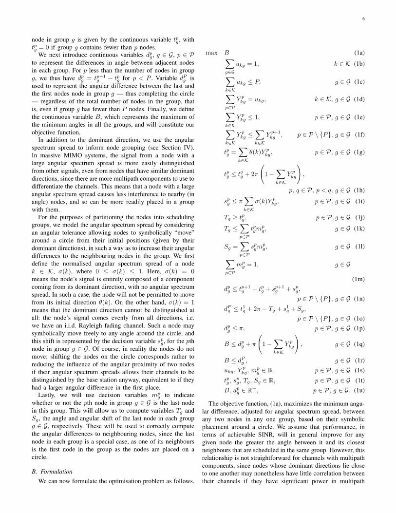
node in group g is given by the continuous variable tpg , withtpg = 0 if group g contains fewer than p nodes.

We next introduce continuous variables dpg , g ∈ G, p ∈ Pto represent the differences in angle between adjacent nodesin each group. For p less than the number of nodes in groupg, we thus have dpg = tp+1

g − tpg for p < P . Variable dPg isused to represent the angular difference between the last andthe first nodes node in group g — thus completing the circle— regardless of the total number of nodes in the group, thatis, even if group g has fewer than P nodes. Finally, we definethe continuous variable B, which represents the maximum ofthe minimum angles in all the groups, and will constitute ourobjective function.

In addition to the dominant direction, we use the angularspectrum spread to inform node grouping (see Section IV).In massive MIMO systems, the signal from a node with alarge angular spectrum spread is more easily distinguishedfrom other signals, even from nodes that have similar dominantdirections, since there are more multipath components to use todifferentiate the channels. This means that a node with a largeangular spectrum spread causes less interference to nearby (inangle) nodes, and so can be more readily placed in a groupwith them.

For the purposes of partitioning the nodes into schedulinggroups, we model the angular spectrum spread by consideringan angular tolerance allowing nodes to symbolically “move”around a circle from their initial positions (given by theirdominant directions), in such a way as to increase their angulardifferences to the neighbouring nodes in the group. We firstdefine the normalised angular spectrum spread of a nodek ∈ K, σ(k), where 0 ≤ σ(k) ≤ 1. Here, σ(k) = 0means the node’s signal is entirely composed of a componentcoming from its dominant direction, with no angular spectrumspread. In such a case, the node will not be permitted to movefrom its initial direction θ(k). On the other hand, σ(k) = 1means that the dominant direction cannot be distinguished atall: the node’s signal comes evenly from all directions, i.e.we have an i.i.d. Rayleigh fading channel. Such a node maysymbolically move freely to any angle around the circle, andthis shift is represented by the decision variable spg , for the pthnode in group g ∈ G. Of course, in reality the nodes do notmove; shifting the nodes on the circle corresponds rather toreducing the influence of the angular proximity of two nodesif their angular spectrum spreads allows their channels to bedistinguished by the base station anyway, equivalent to if theyhad a larger angular difference in the first place.

Lastly, we will use decision variables mpg to indicate

whether or not the pth node in group g ∈ G is the last nodein this group. This will allow us to compute variables Tg andSg , the angle and angular shift of the last node in each groupg ∈ G, respectively. These will be used to correctly computethe angular differences to neighbouring nodes, since the lastnode in each group is a special case, as one of its neighboursis the first node in the group as the nodes are placed on acircle.

B. FormulationWe can now formulate the optimisation problem as follows.

max B (1a)∑g∈G

ukg = 1, k ∈ K (1b)∑k∈K

ukg ≤ P, g ∈ G (1c)∑p∈P

Y pkg = ukg, k ∈ K, g ∈ G (1d)∑

k∈K

Y pkg ≤ 1, p ∈ P, g ∈ G (1e)∑

k∈K

Y pkg ≤

∑k∈K

Y p+1kg , p ∈ P \ {P}, g ∈ G (1f)

tpg =∑k∈K

θ(k)Y pkg, p ∈ P, g ∈ G (1g)

tpg ≤ tqg + 2π

(1−

∑k∈K

Y pkg

),

p, q ∈ P, p < q, g ∈ G (1h)

spg ≤ π∑k∈K

σ(k)Y pkg, p ∈ P, g ∈ G (1i)

Tg ≥ tpg, p ∈ P, g ∈ G (1j)

Tg ≤∑p∈P

tpgmpg, g ∈ G (1k)

Sg =∑p∈P

spgmpg, g ∈ G (1l)∑

p∈Pmp

g = 1, g ∈ G

(1m)

dpg ≤ tp+1g − tpg + sp+1

g + spg,

p ∈ P \ {P}, g ∈ G (1n)

dPg ≤ t1g + 2π − Tg + s1g + Sg,

p ∈ P \ {P}, g ∈ G (1o)dpg ≤ π, p ∈ P, g ∈ G (1p)

B ≤ dpg + π

(1−

∑k∈K

Y pkg

), g ∈ G (1q)

B ≤ dPg , g ∈ G (1r)

ukg, Ypkg, m

pg ∈ B, p ∈ P, g ∈ G (1s)

tpg, spg, Tg, Sg ∈ R, p ∈ P, g ∈ G (1t)

B, dpg ∈ R+, p ∈ P, g ∈ G. (1u)

The objective function, (1a), maximizes the minimum angu-lar difference, adjusted for angular spectrum spread, betweenany two nodes in any one group, based on their symbolicplacement around a circle. We assume that performance, interms of achievable SINR, will in general improve for anygiven node the greater the angle between it and its closestneighbours that are scheduled in the same group. However, thisrelationship is not straightforward for channels with multipathcomponents, since nodes whose dominant directions lie closeto one another may nonetheless have little correlation betweentheir channels if they have significant power in multipath

7

components with different angles of arrival. The minimum an-gular difference that is maximized therefore takes the angularspectrum spread of the nodes’ channels into account, via theconstraints that will be explained below.

The first constraint, (1b), ensures that each node is placedin exactly one group, and constraint (1c) then ensures thatthe number of nodes placed in each group does not exceedthe number of available pilots, P . The decision variables Y p

kg

are used to keep track of which group each node is placedin along with in which order. Hence Y p

kg should be set to 1if node k ∈ K is placed in group g ∈ G at position p ≤ P ,and 0 otherwise. This is enforced using constraints (1d) and(1e). Constraint (1d) requires that exactly one position in groupg ∈ G be assigned to node k ∈ K, if the node is placed inthat group (ukg = 1), and that no positions in the group areassigned to it if it was not placed in that group (ukg = 0).Constraint (1e) ensures that at most one node is assigned toeach position in each group, i.e. a strict ordering is imposedin which two or more nodes cannot occupy the same position.Finally, constraint (1f) prevents gaps in the node ordering foreach group, that is, no position in the group may be filled untilall the preceding positions are filled.

The next three constraints determine the angles and angulartolerances of each node in each group. Constraint (1g) setsthe angle of each node position in each group to be thedominant direction of the node assigned that position, throughthe decision variable tpg . Constraint (1h) ensures that nodesare assigned positions in groups in order of their dominantdirections, that is, a node with a higher angle for its dominantdirection may not be placed earlier in a group than a nodewith a lower angle. The second term on the right-hand sideis used to cancel this constraint when a position in a group isempty, that is, not assigned to any node. Such empty positionsmust occur at the end of the group, thanks to constraint(1f). Constraint (1i) determines the angular tolerance for eachposition in each group, up to a maximum of the angularspectrum spread for the node assigned that position. Thisangular tolerance gives the range within which the node’sangular position can be adjusted.

Because the nodes are symbolically placed on a circle, inwhich an angle of 2π is equivalent to an angle of 0, the lastnode in each group must be treated differently. For the purposeof computing the objective, angular differences between eachsuccessive pair of nodes in each group are considered, andadditionally the angular difference from the last node backaround the remainder of the circle to the first node mustbe included. Constraints (1j)–(1m) are used to find the angleand angular shift for the last node in each group. The binarydecision variable mp

g is set to 1 for the last position in eachgroup, and 0 otherwise. It is not possible to determine inadvance which is the last position in any given group, sincethe groups may have different numbers of nodes assigned tothem.

Constraint (1m) forces only one position in each group tobe selected as the last. To make sure the one selected is indeedthe last, and obtain the angle of the node in the last position,constraints (1j) and (1k) are used. Constraint (1j) requires thatthe angle of the last position in each group g ∈ G, Tg , be

at least as large as all angles in the group tpg . Meanwhile,constraint (1k) requires that Tg be no more than the angle ofthe node selected by the variable mp

g . In this way, mpg can

only feasibly be 1 for the last position in the group. Similarly,variable Sg is set to the angular shift of the last node in thegroup via constraint (1l).

Next, the angular differences between the nodes in eachgroup need to be computed, in constraints (1n)–(1p). Con-straint (1n) sets variable dpg to at most the angular differencebetween the nodes at positions p and p+ 1 in group g, takinginto account their angular tolerances. Since the objective is amaximisation function, equality will be achieved here for anyangular differences that can affect the objective. Constraint(1o) similarly takes the angular difference between the lastand first positions in each group, thus closing the circle. Notethat the variable dPg is used for this last angular difference,regardless of whether or not the last occupied position in thegroup is P or a lower position, due to the group having fewerthan P nodes assigned to it. Constraint (1p) limits all angulardifferences to be at most π, since any difference greater thanthis would imply a smaller angular difference if measured inthe opposite direction around the circle.

We are now ready to compute the objective function usingconstraints (1q) and (1r). These constraints set the objectivefunction value, represented by variable B, to the minimumangular difference of any pair of nodes in any group. Here,again, the last position in each group must be treated separately(constraint (1r)). In constraint (1q), the second term on theright-hand side cancels the constraint for any positions towhich no node has been assigned. Finally, the last threeconstraints in the formulation provide the domains for eachof the decision variables.

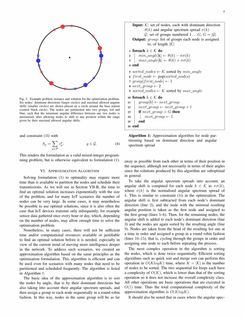
An example problem instance and solution are shown inFig. 3. In this instance, six nodes are partitioned into twogroups. The nodes’ angular shift ranges are indicated inthe figure by the smaller, semi-transparent circles. For thisproblem, most nodes’ ranges do not overlap and so do notaffect the solution: the nodes are placed into the two groupsin an alternating fashion. However, two of the nodes’ rangesoverlap, and in this case the nodes are grouped “out of order”,as they are able to shift within their ranges in order to achievebigger angular differences to the other nodes.

1) Auxiliary Variables: To resolve the bilinearities in con-straints (1k) and (1l), we need to introduce auxiliary variablesvpg = tpgm

pg and zpg = spgm

pg , p ∈ P , g ∈ G, and add the

following constraints to formulation (1).

vpg ≤ tpg, p ∈ P, g ∈ G (2a)

vpg ≤ 2πmpg, p ∈ P, g ∈ G (2b)

vpg ≥ tpg + 2π(mp

g − 1), p ∈ P, g ∈ G (2c)

zpg ≤ spg, p ∈ P, g ∈ G (2d)

zpg ≤ πmpg, p ∈ P, g ∈ G (2e)

zpg ≥ spg + π(mp

g − 1), p ∈ P, g ∈ G. (2f)

Constraint (1k) is then replaced with

Tg ≤∑p∈P

vpg , g ∈ G, (3)

8

Fig. 3. Example problem instance and solution for the optimisation problem.Six nodes’ dominant directions (larger circles) and maximal allowed angularshifts (smaller circles) are shown placed on a circle around the base station(central black circle). The nodes are partitioned into two groups, red andblue, such that the minimum angular difference between any two nodes ismaximized, after allowing nodes to shift to any position within the rangegiven by their maximal allowed angular shifts.

and constraint (1l) with

Sg =∑p∈P

zpg , g ∈ G. (4)

This renders the formulation as a valid mixed-integer program-ming problem, but is otherwise equivalent to formulation (1).

VI. APPROXIMATION ALGORITHM

Solving formulation (1) to optimality may require moretime than is available to partition the nodes and schedule theirtransmissions. As we will see in Section VII-B, the time tofind an optimal solution increases exponentially with the sizeof the problem, and for many IoT scenarios the number ofnodes can be very large. In some cases, it may nonethelessbe possible to use optimal solutions, since it is also often thecase that IoT devices transmit only infrequently, for examplesensor data gathered once every hour or day, which, dependingon the number of nodes, may allow enough time to solve theoptimisation problem.

Nonetheless, in many cases, there will not be sufficienttime and/or computational resources available or justifiableto find an optimal solution before it is needed, especially inview of the current trend of moving more intelligence deeperin the network. To address such scenarios, we created anapproximation algorithm based on the same principles as theoptimisation formulation. This algorithm is efficient and canbe used even for scenarios with many nodes that need to bepartitioned and scheduled frequently. The algorithm is listedin Algorithm 1.

The basic idea of the approximation algorithm is to sortthe nodes by angle, that is by their dominant directions butalso taking into account their angular spectrum spreads, andthen assign a group to each node sequentially in a round robinfashion. In this way, nodes in the same group will be as far

Input: K: set of nodes, each with dominant directionθ(k) and angular spectrum spread σ(k)G: set of groups numbered 1 . . . G, G = |G|

Output: group: list of groups each node is assignedto, of length |K|

1 foreach k ∈ K do2 min angle[k]← θ(k)− πσ(k)3 max angle[k]← θ(k) + πσ(k)4 end

5 sorted nodes← K sorted by min angle6 first node← pop(sorted nodes)7 group[first node]← 18 next group← 29 sorted nodes← K sorted by max angle

10 foreach k ∈ K do11 group[k]← next group12 next group← next group+ 113 if next group > G then14 next group← 115 end16 end

Algorithm 1: Approximation algorithm for node par-titioning based on dominant direction and angularspectrum spread

away as possible from each other in terms of their position inthe sequence, although not necessarily in terms of their anglessince the solutions produced by this algorithm are suboptimalin general.

To take the angular spectrum spreads into account, anangular shift is computed for each node k ∈ K as πσ(k),where σ(k) is the normalised angular spectrum spread ofk. This is similar to constraint (1i) in the optimisation. Theangular shift is first subtracted from each node’s dominantdirection (line 2), and the node with the minimal resultingangular position is taken as the first node and assigned tothe first group (lines 5–6). Then, for the remaining nodes, theangular shift is added to each node’s dominant direction (line3) and the nodes are again sorted by the resulting angle (line9). Nodes are taken from the head of the resulting list one ata time in order and assigned a group in a round robin fashion(lines 10–15), that is, cycling through the groups in order andassigning one node to each before repeating the process.

The most complex operation in the algorithm is sortingthe nodes, which is done twice sequentially. Efficient sortingalgorithms such as quick sort and merge sort can perform thisoperation in O(KlogK) time, where K = |K| is the numberof nodes to be sorted. The two sequential for loops each havea complexity of O(K), which is lower than that of the sortingoperation so it does not increase the overall complexity class.All other operations are basic operations that are executed inO(1) time. Thus the total computational complexity of theapproximation algorithm is O(KlogK).

It should also be noted that in cases where the angular spec-

9

trum spreads are low, such that the resulting angular shifts arelower than the angular differences between nodes’ dominantdirections for most nodes, the list of nodes will already benearly sorted, assuming it is initially provided in order ofnodes’ dominant directions. In this case, the complexity couldbe reduced even further by using bubble sort, which has goodperformance of O(K) for an almost-sorted list where no nodeis out of place by more than one position. In such a case,the complexity of our approximation algorithm also becomesO(K). Since node partitioning based on angles, as proposed inthis paper, is intended for cases where node channels have astrong dominant component and thus interference correlatesstrongly with the directional characteristics of the channel,cases where the angular spectrum spread is low enough touse bubble sort are quite likely to occur. Checking whethera given problem instance fulfills the needed conditions canbe performed in O(K) time, for example by performing thefirst pass of bubble sort and, in case the list is not yetsorted, switching to quick sort or merge sort. Thus, this addedoptimisation for such cases can be included at no additionalcost in terms of computational complexity.

VII. NUMERICAL EVALUATION

We conducted a numerical evaluation to test the per-formance of our optimisation and approximation algorithm,along with two reference algorithms, on randomly generatedinstances of our problem scenario, consisting of a set ofsingle-antenna nodes and an accompanying channel matrix.We compared the performance of the algorithms in terms ofthe achieved minimum, mean, and average SINR. We alsocompared the performance of our approximation with the opti-mal solution in terms of the proportion of the optimal objectivefunction value obtained by the approximation. All sourcecode for our implementations of the optimisation problem,approximation algorithm, channel model, and experiments isavailable online [28].

We generated instances consisting of between 15 and 36nodes, along with a massive MIMO base station with 100antennas, and 12 pilots available in each coherence block.These base station parameters are based on the LuMaMimassive MIMO testbed [29], [30]. The precoding schemeused at the base station in our experiments was MRC. Thiswas chosen because as yet, we have assumed perfect channelestimation, which means that for other precoding methods suchas zero forcing, there will be no interference. In the latter case,all partitions are equivalent as each node’s SINR will be equalto its SNR.

We partitioned the nodes into three groups, and so as thenumber of nodes increased, the number of nodes per groupincreased accordingly. The number of nodes per group isthe most important parameter for determining the achievableSINR, since with more nodes per group the density of nodesis greater and the angular differences between them are lower.Meanwhile, the overall number of nodes is the most importantparameter in terms of the running time of the partitioningalgorithms.

For each number of nodes we generated and tested 20problem instances. The instances were generated using a

TABLE IIPARAMETERS FOR THE NUMERICAL EVALUATION.

Parameter Value

Number of nodes |K| 15 . . . 36, step 3

Number of instances for each numberof nodes

20

Number of pilots P 12

Number of groups 3

Number of base station antennas M 100

Type of antenna array Uniform rectangular arrayPrecoding Maximum ratio combiningCarrier frequency 2.47 GHzNumber of channel clusters 4

Number of channel components percluster

10

Distribution of cluster central angles Uniform 45–135 degreesDistribution of component angleswithin each cluster (vertical and hor-izontal)

Exponential, µ = 7.5 degrees

Component small scale fading distri-bution

Complex normal, µ = 0, σ = 1

Signal-to-noise ratio (for all nodes) 20 dB

channel model based on the Saleh-Valenzuela model [31]and its adaption to MIMO channels [32]. The channel modeland problem instance generation will be further detailed inSection VII-A. As output, the model produces the dominantdirection and angular spectrum spread for each node, alongwith the complete channel matrix giving the channel from eachnode to each antenna.

Using the dominant directions and angular spectrumspreads, we then ran our optimisation algorithm, given informulation (1), on each problem instance. For this we usedthe AMPL modelling language [33] along with the CPLEXoptimisation solver [34], and the optimisation was run ona 12-core server with 2.2 GHZ Intel Xeon ES-2420 CPUsand 24 GiB RAM. The optimal solution was then comparedwith three other node partitioning algorithms. An overviewof the partitioning algorithms is given in Table III. The firstcomparison algorithm was our approximation algorithm, givenin Algorithm 1.

TABLE IIIPARTITIONING ALGORITHMS TESTED.

Node Partitioning Method Description

Optimal Solution Solving formulation (1) to optimality.Approximation algorithm Algorithm 1Clumped partitioning Groups nodes with similar directional prop-

erties together. Worst-case scenario usingdirectional properties.

Power partitioning Groups nodes with similar received powerat the base station together. Partitioningsuitable for use with max-min fair powercontrol. Requires full CSI.

The second comparison algorithm, which we will refer toas clumped node partitioning, is intended to represent a worst-case scenario in which nodes whose channel have similar

10

directional properties are grouped together. In this algorithm,the nodes are first sorted according to their dominant di-rections. Then the first N = |K|

|G| nodes are placed in thefirst group, the next N nodes in the next group, and soon until all nodes have been assigned a group. In our testinstances, the number of nodes is always divisible by thenumber of groups, so there will be no nodes left over withthis procedure, and all groups will contain the same numberof nodes. Clumped partitioning gives an indication of thedetriment to performance that might be caused by a poor nodepartition with respect to the directional channel properties weconsider.

The third comparison algorithm, called power partitioning,uses the entire channel matrix as input, rather than only thedirectional properties of the node channels, and thus is used asa comparison against the case where full channel informationis obtained before partitioning. This is not feasible in practice.This is firstly because it would require partitioning nodesafter they have transmitted pilots in the coherence block inwhich they are to transmit, whereas in reality pilots can onlybe allocated to nodes after partitioning has been performed.Secondly, in an IoT scenario, the signalling cost for collectingchannel information in order to perform partitioning is toohigh; our aim is to provide a partitioning strategy with lowenergy usage on the end devices.

Power partitioning sorts the nodes according to the receivedpower of their channels at the base station, and then groupsthose nodes with similar power levels. Similarly to clumpedpartitioning, this is done by assigning the N = |K|

|G| nodeswith the highest received power to the first group, the next Nhighest power nodes to the next group, and so on. For MRCprecoding, the interference scales with the interfering nodes’received power [2]. Power partitioning thus provides a reason-ably fair partition in which nodes experience interference onlyfrom other nodes with similar received power.

This is similar to max-min fair power control [35], inwhich a common SINR is achieved for all users by adjustingtheir transmission power such that the received power fromeach user at the base station is equal. In the absence oftransmission power control, fair performance — in the formof equal SINR — cannot be achieved exactly, however powerpartitioning comes as close as possible using only partitioning.If partitioning were to then be combined with transmissionpower control, power partitioning would then provide thebest conditions for carrying out max-min fair power controlsince the users in each group will have as similar receivedpower levels as possible before applying the power controlalgorithm. For these reasons, power partitioning provides agood comparison algorithm making use of full CSI for our usecase, in which the goal is to maximise the minimum SINR,rather than provide the maximum rum rate as in other userselection algorithms (see Section III).

Finally, we computed the SINR achieved for each node forthe partitions produced by each of the algorithms, under MRCprecoding. Here, the interfering nodes are only those that wereplaced in the same group, as it is these nodes that will transmitin the same coherence block. We then took the minimum SINRobtained by any node in any group as our primary performance

metric, however we also examined the mean and maximumSINR across all the nodes.

A. Channel Model

To generate each problem instance, we used the channelmodel from [32], which is in turn based on the Saleh-Valenzuela model [31]. In this model, nodes’ signals arrive atthe base station as multiple components grouped into a numberof different clusters. Clusters can for example represent objectsin the environment that the nodes’ signals have reflectedfrom (possibly multiple times) before arriving at the basestation. Each cluster has a central angle of arrival to the basestation, around which its constituent components fall. In ourexperiments, we used four clusters, each with ten components,and the cluster central angles were drawn from a uniformrandom distribution between 45 degrees and 135 degrees,where 90 degrees is perpendicular to the plane of the antennaarray, which was a uniform rectangular array. The componentswere distributed around these central angles according toexponential distributions with mean 7.5 degrees, one in eachof the vertical and horizontal planes, with a 0.5 probability ofa given component lying in either direction from the centralangle in each plane. Each component is subject to small scalefading following a complex normal distribution with mean0 and standard deviation 1. Finally, the node channels arenormalised such that the expected power of each node’s signalis 1.

In [32], clusters are generated homogeneously, howeverour use case concerns channels that exhibit clear dominantdirections. To model this, for each node, we amplified thecluster with the highest power, by multiplying it by a scalardrawn uniformly randomly from the interval [2.0, 6.0]. Thiscould represent either the line of sight part of the node’schannel, or a set of components reflected from a highlyreflective surface, if there is no line of sight path betweenthe base station and the node. The node channel was thenre-normalised to ensure the expected power was still 1.0. Inthis way, we generated channels with a more clear dominantcomponent and lower angular spectrum spread than in [32].

The dominant direction for each node was taken to be thecentral angle of the dominant cluster. To compute the angularspectrum spread, we used the Rician K-factor, adjusted for theangular distribution of the generated clusters for each node.For each node k ∈ K, the angular spectrum spread σ(k) wascomputed as

σ(k) = Ψ(k)

(1.0− P (Cd(k))∑

c∈{C(k)\Cd(k)} P (c)

), (5)

where C(k) is the set of clusters in node k’s channel, Cd(k) ∈C(k) is the dominant cluster, P (c) is the received signal powerat the base station of cluster c ∈ C(k), and Ψ(k) is thenormalised angular spread of the clusters, computed as

Ψ(k) =max{ψ(c) : c ∈ C(k)} −min{ψ(c) : c ∈ C(k)}

2π,

(6)where ψ(c) is the central angle of cluster c ∈ C(k), in radians.

11

15 18 21 24 27 30 33 36Number of nodes

0.0

0.5

1.0

1.5

2.0

2.5

3.0

3.5

SINR

OptimalApproximationClumpedPower

Fig. 4. Minimum SINR for different numbers of nodes and node partitioningmethods.

We thus find the share of the total signal power in thedominant component (the Rician K-factor), and take its com-plement, since a lower K-factor implies a higher angularspectrum spread, and vice versa. We then adjust this accordingto how the clusters are distributed across the angular spectrum,by multiplying by Ψ(k), the difference between the largestand smallest central angles. This is because, as defined inSection V, an angular spectrum spread of 1.0 should indicatea channel uniformly spread across all angles, that is, aroundthe entire circle, so in cases where the clusters are groupedin a certain direction, the maximum angular spectrum spreadis reduced accordingly. Since we have considered a uniformrectangular antenna array in our experiments, the array cannotreceive signals from all directions. We have used bounds of45 and 135 degrees so as to place all clusters in the region ofbest response for the antenna array.

B. Results

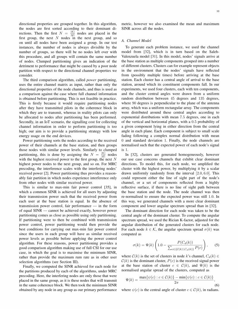
The minimum, average, and maximum SINRs obtained foreach algorithm and number of nodes are shown in Fig. 4–6 respectively. In the figures, the values shown are the av-erages across all instances for each number of nodes, with95% confidence intervals. As expected, clumped partitioningperforms the worst, with the SINR decreasing as the numberof nodes increases. The results even show that a bad groupingof nodes can impact the SINR dramatically, degrading theSINR on average by > 5 dB for 15–20 nodes per groupin the considered scenarios. This shows the potential poorperformance that may occur if a partition is chosen thatdoes not take into account the directional properties of thenodes’ channels. All of the other algorithms substantiallyoutperformed clumped partitioning on all three SINR metrics.

The performance of the other three algorithms was similar.Even though the optimisation and approximation algorithmused only the two parameters of dominant direction and an-gular spectrum spread, they were nonetheless able to match theperformance of power partitioning, which used the full channel

15 18 21 24 27 30 33 36Number of nodes

0.0

2.5

5.0

7.5

10.0

12.5

15.0

17.5

20.0

SINR

OptimalApproximationClumpedPower

Fig. 5. Average SINR for different numbers of nodes and node partitioningmethods.

15 18 21 24 27 30 33 36Number of nodes

0

10

20

30

40

50

60

70

80SINR

OptimalApproximationClumpedPower

Fig. 6. Maximum SINR for different numbers of nodes and node partitioningmethods.

information for each node. This is promising, especially forIoT scenarios, as it demonstrates that an effective node parti-tion can be achieved even with only little information aboutthe nodes’ channels. Moreover, the directional properties wehave used will be relatively stable over time for static or slow-moving nodes, meaning that the signalling needed to facilitatenode partitioning is reduced, as channel information need onlybe collected from the nodes occasionally. In the best case,each time nodes transmit, the channel information obtainedfrom their collected pilot signals can be used to computethe next node partition, even in cases where nodes transmitonly infrequently, as in many sensor networks and monitoringapplications.

In many cases, we observe a relatively large variance in theSINRs obtained for all algorithms. This is because while bothour partitioning approaches and power partitioning attempt toreduce inter-node interference, a true optimal partition wouldrequire actually computing the instantaneous interference be-

12

15 18 21 24 27 30 33 36Number of nodes

0

2

4

6

8

10

Objective (degrees)

OptimalApproximation

Fig. 7. Objective function value for partitioning with optimisation problemand with approximation algorithm, for different numbers of nodes.

tween the nodes. This depends on the correlations betweenthe users’ channels, and while both the directional channelproperties (for our approach) and the instantaneous power (forpower partitioning) correlate with the inter-node interference,they do not perfectly capture it. The variance is greater whenthe number of nodes is lower, since with fewer nodes theprobability of the nodes being more unevenly distributedacross the angular spectrum increases, leading to a higherproportion of unusual cases.

From the figures, we can see that the optimisation andapproximation algorithm performed similarly, with the approx-imation even obtaining a higher SINR in some cases, althoughthe difference between the two is only statistically significantin one case, for the minimum SINR for 33 nodes. The reasonthat the approximation algorithm can achieve better perfor-mance than the optimisation is again that here we measureperformance in terms of SINR, calculated from the completenode channels, whereas the two algorithms — optimisationand approximation — have only reduced channel informationavailable to them in the form of the dominant directions andangular spectrum spreads. As can be seen in Fig. 7, in terms ofthe objective function value obtained, the optimisation alwaysoutperforms the approximation, as expected. Across all thecases tested, the approximation algorithm achieves an averageof 81% of the optimal objective function value.

Fig. 8 shows the time to solve formulation (1) to optimality,versus the number of nodes. As is typical for this kind ofcombinatorial optimisation problem, the solution time growsexponentially with the problem instance size (note that thesolution times are shown on a log scale). For small instancesof 15 nodes, the optimisation takes less than ten seconds torun, which is feasible in practice for IoT scenarios where nodestransmit on the order of minutes or higher. However, for largerinstances, it would not be feasible to use the optimisation;the largest solution time observed was 1232518.65 — morethan 14 days —- and realistic IoT scenarios can have a fargreater number of nodes than we tested here. As a comparison,

15 18 21 24 27 30 33 36Number of nodes

101

102

103

104

105

Solu

tion

time

(s)

Fig. 8. Solution time vs. number of nodes.

our Python implementation of the approximation algorithmran in less than 0.1 ms for all cases tested. For practicaldeployments, the approximation algorithm is thus a moreappropriate solution.

VIII. CONCLUSION AND FUTURE WORK

In this paper we have developed a new method for nodegrouping in massive MIMO systems based on directionalchannel characteristics. The two channel properties we use,dominant direction and angular spectrum spread, are typicallystable over large time scales, when compared to the fullchannel information that should be updated at the rate of thecoherence time of the channel. Our approach hence enablesgrouping of low-power IoT devices with minimal signallingoverhead, even when the devices’ measurement and transmis-sion periods are long. We provided both a mixed-integer opti-misation formulation and an efficient approximation algorithmto perform the node grouping. In our numerical evaluation, wedemonstrated that our approach provides good performance,in terms of the minimum SINR achieved for any node inany group, comparable to a reference method exploiting fullchannel state information. Our assessment also highlightsthat a partitioning that groups nodes with similar directionalproperties together can have a particularly detrimental effecton link quality due to the interference generated by MRCprecoding.

A light signalling user grouping approach as we havedemonstrated in this paper is valuable for any situation wheresignalling overhead is significant. This will be the case whenthere are a very large number of nodes, as in IoT scenarios.At the end devices, reducing signalling overhead also reducesenergy usage, which is critical for battery powered IoT de-vices.

In future work, we aim to close the loop by performingmeasurements in which we measure nodes’ channels andthen apply our solutions and measure the performance of theresulting node groups. We also plan to extend our method totake into account errors in the directional channel information.

13

This will not only make the method more robust in case ofmeasurement errors, but also cater to mobile nodes, sinceas a node moves, its directional information changes, thuseffectively producing an error compared to the last time thisinformation was measured.

REFERENCES

[1] 3GPP, “Further advancements for e-utra physical layer aspects,” TR36.814, 2010.

[2] T. L. Marzetta, E. G. Larsson, H. Yang, and H. Q. Ngo, Fundamentalsof Massive MIMO. Cambridge University Press, 2016.

[3] E. Fitzgerald, M. Pioro, and F. Tufvesson, “Massive MIMO optimizationwith compatible sets,” IEEE Transactions on Wireless Communications,vol. 18, no. 5, pp. 2794–2812, 2019.

[4] X. Gao, O. Edfors, F. Rusek, and F. Tufvesson, “Massive MIMOperformance evaluation based on measured propagation data,” IEEETransactions on Wireless Communications, vol. 14, no. 7, pp. 3899–3911, 2015.

[5] X. Gao, O. Edfors, F. Tufvesson, and E. G. Larsson, “Massive MIMOin real propagation environments: Do all antennas contribute equally?”IEEE Transactions on Communications, vol. 63, no. 11, pp. 3917–3928,2015.

[6] S. Gunnarsson, J. Flordelis, L. Van der Perre, and F. Tufvesson, “Channelhardening in massive MIMO-A measurement based analysis,” in 2018IEEE 19th International Workshop on Signal Processing Advances inWireless Communications (SPAWC), June 2018, pp. 1–5.

[7] G. Dimic and N. D. Sidiropoulos, “On downlink beamforming withgreedy user selection: performance analysis and a simple new algo-rithm,” IEEE Transactions on Signal processing, vol. 53, no. 10, pp.3857–3868, 2005.

[8] J. Wang, D. J. Love, and M. D. Zoltowski, “User selection with zero-forcing beamforming achieves the asymptotically optimal sum rate,”IEEE Transactions on Signal Processing, vol. 56, no. 8, pp. 3713–3726,2008.

[9] S. Huang, H. Yin, J. Wu, and V. C. Leung, “User selection for multiuserMIMO downlink with zero-forcing beamforming,” IEEE Transactionson Vehicular Technology, vol. 62, no. 7, pp. 3084–3097, 2013.

[10] W.-L. Shen, K. C.-J. Lin, M.-S. Chen, and K. Tan, “SIEVE: Scalableuser grouping for large MU-MIMO systems,” in IEEE Conference onComputer Communications (INFOCOM). IEEE, 2015, pp. 1975–1983.

[11] R. Tian, Y. Liang, X. Tan, and T. Li, “Overlapping user grouping iniot oriented massive mimo systems,” IEEE Access, vol. 5, pp. 14 177–14 186, 2017.

[12] H. Zhou and M. Tao, “Joint multicast beamforming and user groupingin massive MIMO systems,” in IEEE International Conference onCommunications (ICC). IEEE, 2015, pp. 1770–1775.

[13] M. Benmimoune, E. Driouch, W. Ajib, and D. Massicotte, “Joint trans-mit antenna selection and user scheduling for massive MIMO systems,”in 2015 IEEE Wireless Communications and Networking Conference(WCNC). IEEE, 2015, pp. 381–386.

[14] X. Guozhen, L. An, J. Wei, X. Haige, and L. Wu, “Joint user schedulingand antenna selection in distributed massive MIMO systems with limitedbackhaul capacity,” China Communications, vol. 11, no. 5, pp. 17–30,2014.

[15] G. Lee and Y. Sung, “A new approach to user scheduling in massivemulti-user MIMO broadcast channels,” IEEE Transactions on Commu-nications, vol. 66, no. 4, pp. 1481–1495, 2017.

[16] S. E. Hajri, M. Assaad, and G. Caire, “Scheduling in massive mimo:User clustering and pilot assignment,” in 2016 54th Annual AllertonConference on Communication, Control, and Computing (Allerton).IEEE, 2016, pp. 107–114.

[17] Y. Xu, G. Yue, and S. Mao, “User grouping for massive MIMO in FDDsystems: New design methods and analysis,” IEEE Access, vol. 2, pp.947–959, 2014.

[18] J. Nam, A. Adhikary, J.-Y. Ahn, and G. Caire, “Joint spatial divisionand multiplexing: Opportunistic beamforming, user grouping and sim-plified downlink scheduling,” IEEE Journal of Selected Topics in SignalProcessing, vol. 8, no. 5, pp. 876–890, 2014.

[19] E. Castaneda, A. Silva, A. Gameiro, and M. Kountouris, “An overviewon resource allocation techniques for multi-user MIMO systems,” IEEECommunications Surveys & Tutorials, vol. 19, no. 1, pp. 239–284, 2016.

[20] A. Adhikary, J. Nam, J.-Y. Ahn, and G. Caire, “Joint spatial divisionand multiplexingthe large-scale array regime,” IEEE transactions oninformation theory, vol. 59, no. 10, pp. 6441–6463, 2013.

[21] H. Huh, S.-H. Moon, Y.-T. Kim, I. Lee, and G. Caire, “Multi-cell MIMOdownlink with cell cooperation and fair scheduling: A large-system limitanalysis,” IEEE Transactions on Information Theory, vol. 57, no. 12, pp.7771–7786, 2011.

[22] L. Liu, E. G. Larsson, W. Yu, P. Popovski, C. Stefanovic, and E. De Car-valho, “Sparse signal processing for grant-free massive connectivity: Afuture paradigm for random access protocols in the internet of things,”IEEE Signal Processing Magazine, vol. 35, no. 5, pp. 88–99, 2018.

[23] E. De Carvalho, E. Bjornson, J. H. Sørensen, P. Popovski, and E. G.Larsson, “Random access protocols for massive MIMO,” IEEE Commu-nications Magazine, vol. 55, no. 5, pp. 216–222, 2017.

[24] E. Bjornson, E. De Carvalho, E. G. Larsson, and P. Popovski, “Randomaccess protocol for massive MIMO: Strongest-user collision resolution(SUCR),” in Proc. IEEE International Conference on Communications(ICC). IEEE, 2016, pp. 1–6.

[25] J. H. Sørensen, E. De Carvalho, and P. Popovski, “Massive MIMO forcrowd scenarios: A solution based on random access,” in 2014 GlobecomWorkshops (GC Wkshps). IEEE, 2014, pp. 352–357.

[26] E. De Carvalho, E. Bjornson, E. G. Larsson, and P. Popovski, “Randomaccess for massive MIMO systems with intra-cell pilot contamination,”in 2016 IEEE International Conference on Acoustics, Speech and SignalProcessing (ICASSP). IEEE, 2016, pp. 3361–3365.

[27] A. Biswas and S. Reisenfeld, “New high resolution direction of arrivalestimation using compressive sensing,” in 2017 IEEE 22nd InternationalWorkshop on Computer Aided Modeling and Design of CommunicationLinks and Networks (CAMAD). IEEE, 2017, pp. 1–6.

[28] E. Fitzgerald, M. Pioro, H. Tataria, G. Callebaut, S. Gunnarsson, andL. Van der Perre, “Pizza: User partitioning for low power IoT networkswith massive MIMO,” https://bitbucket.org/EIT networking/pizza.

[29] J. Vieira, S. Malkowsky, K. Nieman, Z. Miers, N. Kundargi, L. Liu,I. Wong, V. Owall, O. Edfors, and F. Tufvesson, “A flexible 100-antennatestbed for massive MIMO,” in Proc. Globecom Workshops (GC Wkshps)2014. IEEE, 2014, pp. 287–293.

[30] S. Malkowsky, J. Vieira, L. Liu, P. Harris, K. Nieman, N. Kundargi, I. C.Wong, F. Tufvesson, V. Owall, and O. Edfors, “The worlds first real-timetestbed for massive MIMO: Design, implementation, and validation,”IEEE Access, vol. 5, pp. 9073–9088, 2017.

[31] A. A. Saleh and R. Valenzuela, “A statistical model for indoor multipathpropagation,” IEEE Journal on selected areas in communications, vol. 5,no. 2, pp. 128–137, 1987.

[32] O. El Ayach, S. Rajagopal, S. Abu-Surra, Z. Pi, and R. W. Heath,“Spatially sparse precoding in millimeter wave MIMO systems,” IEEEtransactions on wireless communications, vol. 13, no. 3, pp. 1499–1513,2014.

[33] R. Fourer and B. Kernighan, AMPL: A Modeling Language for Mathe-matical Programming. Duxbury Press, 2002.

[34] “CPLEX optimizer,” https://www.ibm.com/analytics/cplex-optimizer,accessed on 2019-12-20.

[35] E. Bjornson, E. G. Larsson, and T. L. Marzetta, “Massive MIMO:Ten myths and one critical question,” IEEE Communications Magazine,vol. 54, no. 2, pp. 114–123, 2016.