A Linear Parameter-Varying Control Method for Inline Wheel Systems by Ronald Grant Smith A thesis submitted in partial fulfillment of the requirements for the degree of Master of Science in Engineering (Electrical Engineering) in the University of Michigan-Dearborn 2021 Master’s Thesis Committee: Associate Professor Sridhar Lakshmanan, Committee Chair Lecturer II Randy Boone Lecturer I Paul Muench
Transcript
A Linear Parameter-Varying Control Method for Inline Wheel Systems
by
Ronald Grant Smith
A thesis submitted in partial fulfillment of the requirements for the degree of
Master of Science in Engineering (Electrical Engineering)
in the University of Michigan-Dearborn 2021
Master’s Thesis Committee: Associate Professor Sridhar Lakshmanan, Committee Chair Lecturer II Randy Boone Lecturer I Paul Muench
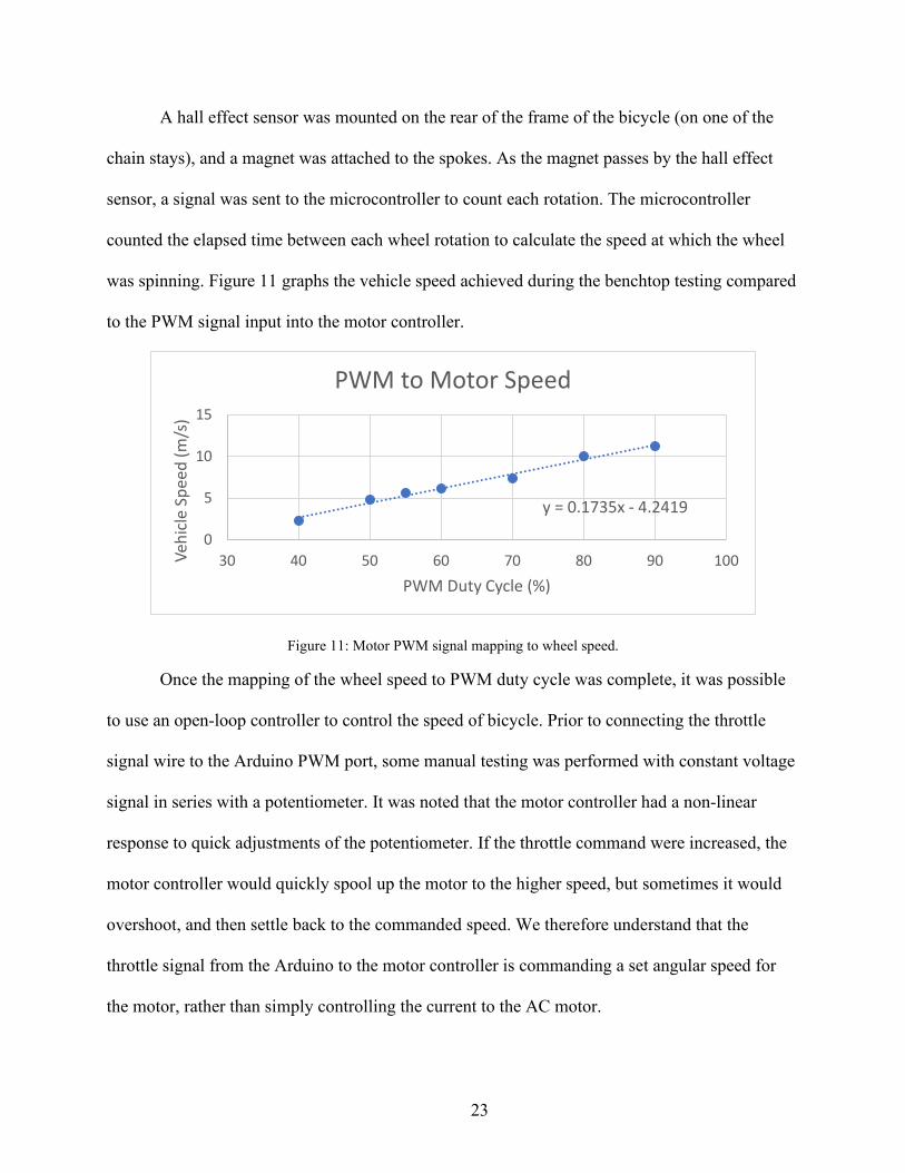
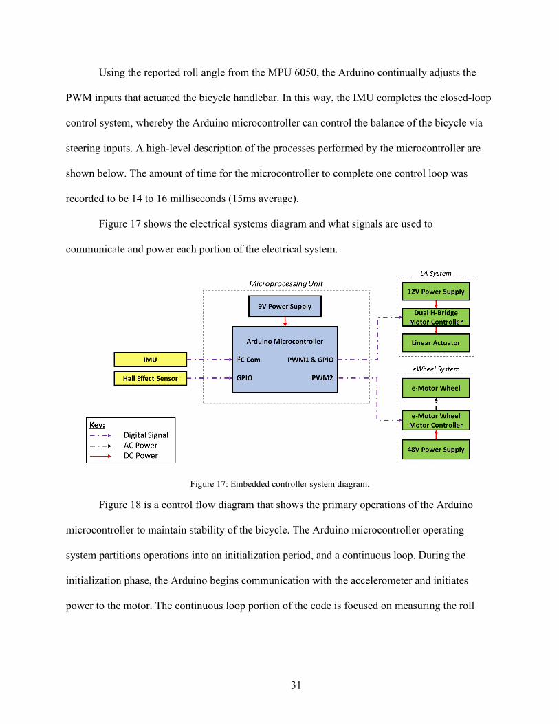
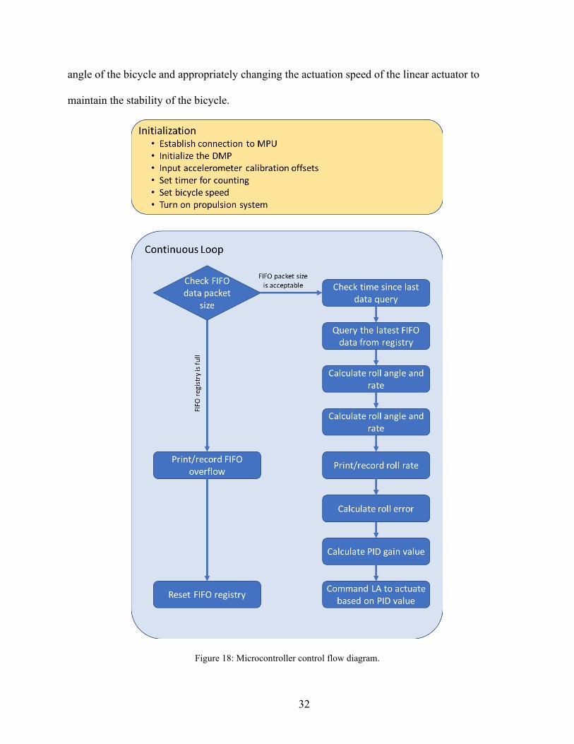
Noting that the right-hand side of the equation is governed by inputs from the ground
plane, a bicycle can be considered as an inverted pendulum mounted on a laterally moving
platform [20]. By relating the lateral acceleration and yaw of the bicycle back to the steering
angle, it is shown that the stability of the bicycle can be completely controlled by the steering
angle and forward velocity of the bicycle:
(𝐼𝐼1 + 𝑚𝑚ℎ2)�̈�𝜃 − 𝑚𝑚𝑚𝑚ℎ𝜃𝜃 = −𝑚𝑚ℎ𝑎𝑎 + 𝑏𝑏
(𝑏𝑏𝛿𝛿�̇�𝑓𝑈𝑈 + 𝛿𝛿𝑓𝑓𝑈𝑈2) (6)
Where:
𝐼𝐼1 – Inertia of the bicycle about the roll-axis of the bicycle 𝑚𝑚 – Mass of the entire autonomous bicycle system ℎ – Height of the center of gravity (above the ground plane) �̈�𝜃 – Second derivative of the roll angle a – Distance from the front axle to the center of gravity (ground plane projection) b – Distance from the rear axle to the center of gravity (ground plane projection) 𝛿𝛿𝑓𝑓 – Front fork steering angle 𝑈𝑈 – Forward velocity of the bicycle
39
Note in the stability equation that if the bicycle is stationary (the speed is zero), the actuation of
the has no bearing of the roll angle on the bicycle. Also, the higher the speed bicycle, the more
sensitive the roll rate is to the steering angle and steering rate.
3.3 Stability Analysis
To simplify the stability analysis, Karnopp defined the following constants:
𝜏𝜏12 =
(𝐼𝐼1 + 𝑚𝑚ℎ2)𝑚𝑚𝑚𝑚ℎ
, 𝜏𝜏2 =𝑏𝑏𝑈𝑈
, 𝜏𝜏3 =𝑎𝑎𝑈𝑈
,𝐾𝐾 =𝑈𝑈2
𝑚𝑚(𝑎𝑎 + 𝑏𝑏) (7)
The transfer function is therefore shown as follows:
(𝜏𝜏12)�̈�𝜃 − 𝜃𝜃 = −𝐾𝐾(𝜏𝜏2𝛿𝛿�̇�𝑓 + 𝛿𝛿𝑓𝑓) (8)
Thus, the characteristic equation for the system is of the form 𝜏𝜏12𝑐𝑐2 − 1 = 0. With two
poles in on the real axis mirrored at ± 1𝜏𝜏1
(the same as an inverted pendulum). The stability of the
system can be improved and by increasing the height of the center of gravity, the mass, or
increasing the rotational inertia of the bicycle. This model of the bicycle explains how the
steering angle and roll angle of the bicycle are interrelated and explains the steady-state motion
of a bicycle. The transfer function produced, uses the steering angle as the input lean of the
system.
It is important to note that in this simple model of the bicycle, the bicycle is not capable
of self-stabilizing. The primary reason for this is that the front fork dynamics have been ignored.
As noted in [12], when a bicycle is in a lean, the tire-road contact forces exhibit a torque on the
bicycle front fork. On a bicycle with a positive trail, the contact forces exhibit a counter-torque
on the front fork. As the speed of the bicycle increases, so do the tire-road contact forces. Since
the steering angle and roll angle of the bicycle are interrelated, the counter-torque on the front
fork results in negative feedback to the roll angle of the bicycle, provided that the torque is large
40
enough to change the steering angle. Therefore, all bicycles with a positive trail can be self-
stabilizing under certain speed and leaning conditions. This explains why a skilled bicycle rider
can ride the bicycle hands free.
Is it appropriate to use a bicycle model that ignores the self-stabilizing impact of the front
fork geometry?
First, the control method proposed utilizes a linear actuator which is mechanical joined to
the front steering fork. The linear actuator has minimal back-drivability; therefore, any counter
torque effects from the front fork tire contact will be mitigated because they will not be large
enough to change the steering angle of the front fork. While the counter-torque forces on the
handlebar will still impact the path of the vehicle (they still impact the effective steering angle of
the bicycle), it will not improve the bicycle lean stability. Second, the bicycle used for
experimental validation of the control method is a “neutral” bicycle, meaning the trail on the
front fork is minimal. Finally, the front fork geometry improves (not decreases) the stability of
the system, it is a conservative assumption to ignore its impact on the steady-state stability of the
system.
3.3.1 Stability Modeling
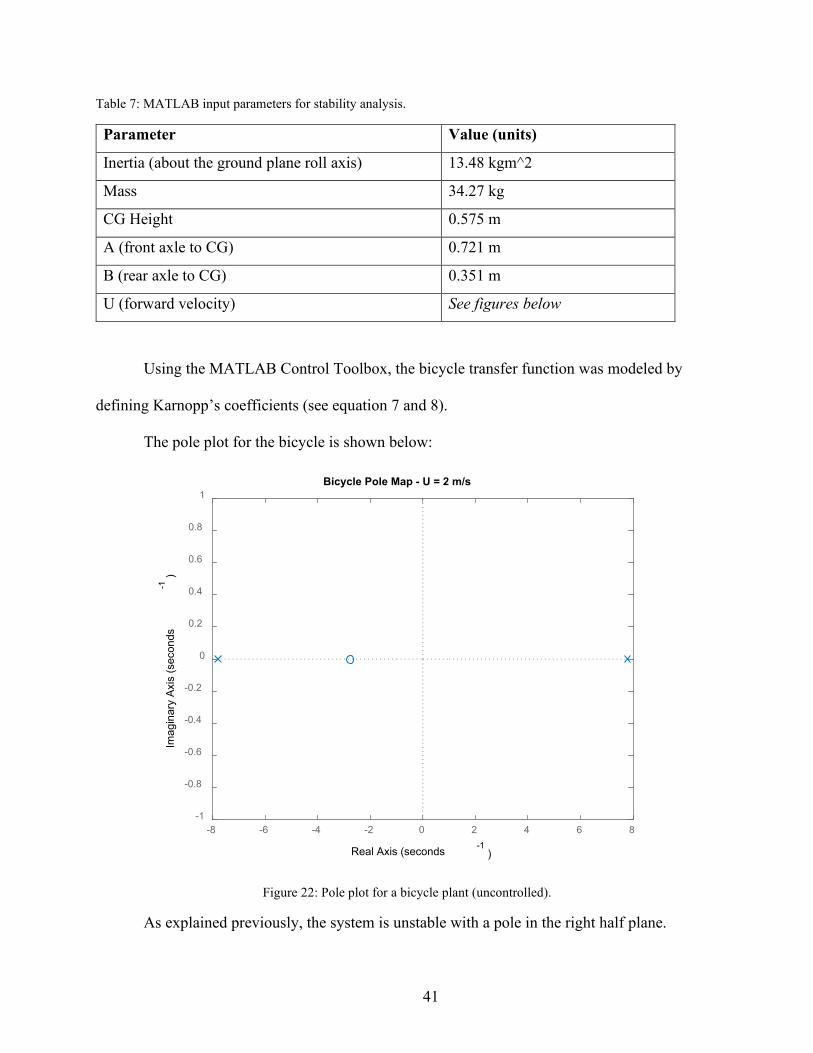
The prototype bicycle system was measured and weighed. Table 7 shows the input
parameters which were used to model the system in MATLAB.
41
Table 7: MATLAB input parameters for stability analysis.
Parameter Value (units)
Inertia (about the ground plane roll axis) 13.48 kgm^2
Mass 34.27 kg
CG Height 0.575 m
A (front axle to CG) 0.721 m
B (rear axle to CG) 0.351 m
U (forward velocity) See figures below
Using the MATLAB Control Toolbox, the bicycle transfer function was modeled by
defining Karnopp’s coefficients (see equation 7 and 8).
The pole plot for the bicycle is shown below:
Figure 22: Pole plot for a bicycle plant (uncontrolled).
As explained previously, the system is unstable with a pole in the right half plane.
-8 -6 -4 -2 0 2 4 6 8-1
-0.8
-0.6
-0.4
-0.2
0
0.2
0.4
0.6
0.8
1Bicycle Pole Map - U = 2 m/s
Real Axis (seconds -1)
Imag
inar
y Ax
is (s
econ
ds-1
)
42
3.4 Controller Design
As outlined in 3.3, the geometry and inertial properties of the bicycle impact the system
stability. However, the only controllable variables are:
• Actuation of the front fork (steering angle and steering rate), and
• Forward velocity of the bicycle
Chapter 2 notes various works on single-track vehicle stability control through front fork
actuation. Schwab gives a good summary of control methods that have been successfully
implemented [7, see Section 3]. These include optimal (LQR) controllers, PID and LPV
𝑈𝑈𝑃𝑃𝑃𝑃𝑃𝑃 – The control signal output from the microcontroller at each time step 𝑈𝑈𝑃𝑃𝑃𝑃 – The control signal output from the microcontroller at each time step 𝜃𝜃(𝑡𝑡) – Roll angle at each time step (measured) 𝑒𝑒𝜃𝜃 –Roll angle error at each time step (desired - measured) �̇�𝑒𝜃𝜃 – Rate of change of roll angle error at each time step (calculated from 𝑒𝑒𝜃𝜃) 𝐾𝐾𝑝𝑝 – Proportional gain constant 𝐾𝐾𝑝𝑝 – Derivative gain constant 𝐾𝐾𝑖𝑖 – Integral gain constant
50
The controller could be considered somewhat of a hybrid controller since it used a
different control strategy (PD vs. PID) depending on the state of the system.
51
Chapter 4 Experimental Results
The experimental objectives were to achieve the following milestones:
1. Demonstrate the use of a linear actuator to control the front handlebar as a viable method
for front fork steering actuation.
2. Validate the control laws outlined in the previous section.
3. Show that through gain scheduling, the system could be stabilized at a range of speeds
under power.
4.1 Test Setup and PID Tuning Process
The first round of testing was performed without the propulsion system installed. With
less mass on the bicycle, it was possible to give the bicycle enough momentum for it to travel a
measurable distance with a strong push and give the stabilizing controller time to (re)act. An
entire catalog of PID tuning processes is described from both industry and academic sources
[58],[59],[60]. Given the high number on non-linearities in a single-track vehicle system, this
thesis determined to perform a trial-and-error method that is comparable (in some ways) to the
Ziegler-Nichols tuning method. The process is outlined below:
1. Set the derivative and integral constants to zero.
2. Increase the proportional gain constant until the controller can correct an initial fall to
one side.
3. Increase the derivative gain constant until the controller sufficiently dampens oscillatory
motions and can achieve a steady-state motion.
4. Add the integrator constant to correct for small steady-state errors.
5. Trial higher derivative gain constants to increase response time and minimize overshoot.
52
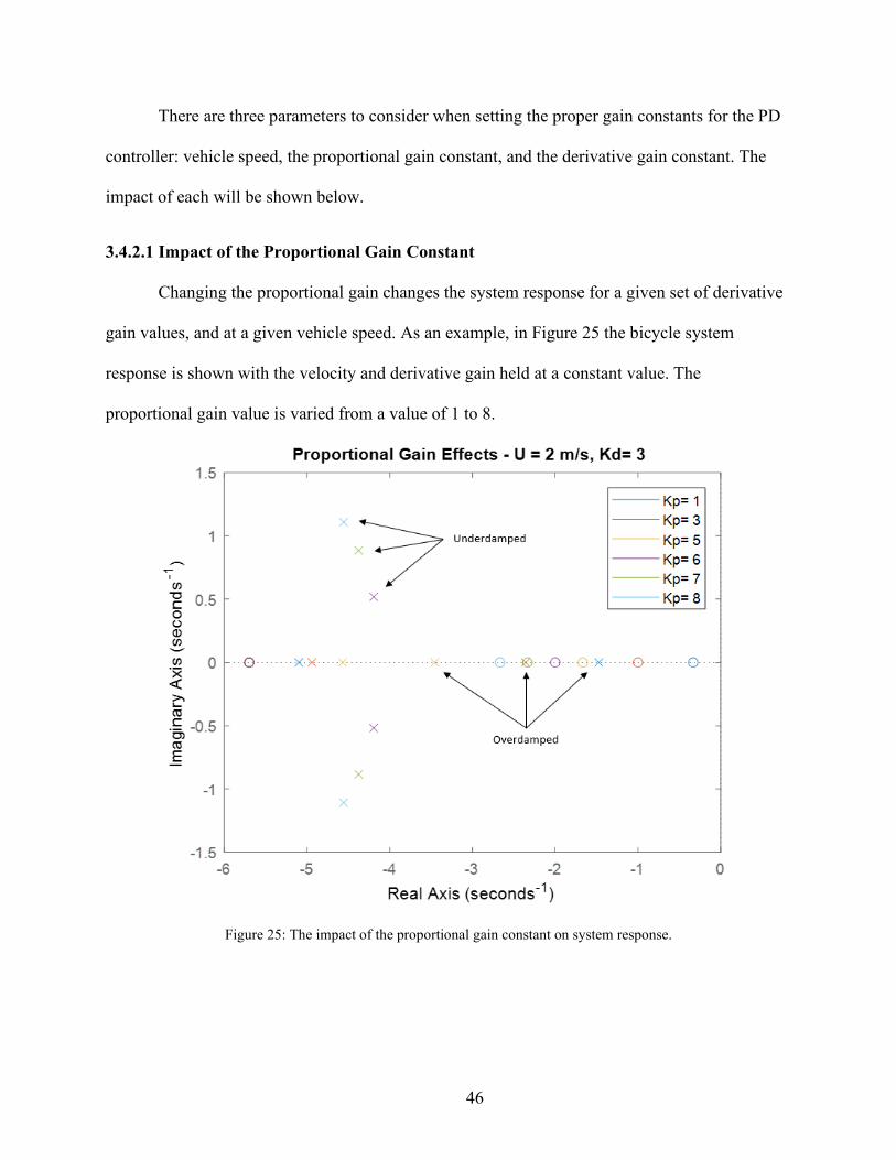
The Zeigler-Nichols method and other methods recommended for manual tuning
generally begin by isolating a single constant (usually the proportional gain constant) and
increasing it until the targeted step response is achieved [60],[61]. In the case of stabilizing a
single-track vehicle, it has not been proved possible to stabilize the system with proportional
gain alone. Therefore, it was thought that once the proportional controller was able to catch the
bicycle system from falling to one side, it would be a sufficient starting point to add in the
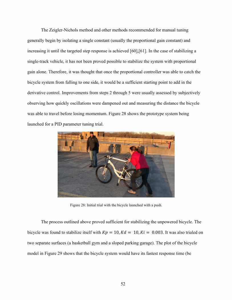
derivative control. Improvements from steps 2 through 5 were usually assessed by subjectively
observing how quickly oscillations were dampened out and measuring the distance the bicycle
was able to travel before losing momentum. Figure 28 shows the prototype system being
launched for a PID parameter tuning trial.
Figure 28: Initial trial with the bicycle launched with a push.
The process outlined above proved sufficient for stabilizing the unpowered bicycle. The
bicycle was found to stabilize itself with 𝐾𝐾𝐾𝐾 = 10,𝐾𝐾𝐾𝐾 = 10,𝐾𝐾𝑐𝑐 = 0.003. It was also trialed on
two separate surfaces (a basketball gym and a sloped parking garage). The plot of the bicycle
model in Figure 29 shows that the bicycle system would have its fastest response time (be
53
critically damped) in the 1m/s to 1.5m/s (2.2-3.4mph) speed range, which is achievable with a
strong push.
Figure 29: System response with the experimental gain values.
The initial tests and PID tuning process proved that the bicycle could be stabilized by a
linear actuator and that the PD/PID hybrid control law proposed functioned as intended.
4.2 Testing Under Self-Propulsion
After the initial control testing was accomplished with the bicycle unpowered, the
motorized wheel and propulsion power system were added to the bicycle. The propulsion system
added significant weight to the rear of the bicycle which shifted the center of gravity closer to the
rear axle and increased the overall inertia of the system.
The bicycle system was now sufficiently heavy that it was difficult for a person to catch
the bicycle if it started to fall. Modified training wheels were installed to prevent the bicycle
from falling over. When system testing began, the control parameters from the previous testing
-9 -8 -7 -6 -5 -4 -3 -2 -1 0-3
-2
-1
0
1
2
3
U= 0.5 m/s
U= 1 m/s
U= 1.5 m/s
U= 2 m/s
U= 2.5 m/s
U= 3 m/s
Effect of Speed on System Response - Kp = 10, Kd = 10
Real Axis (seconds -1)
Imag
inar
y Ax
is (s
econ
ds-1
)
54
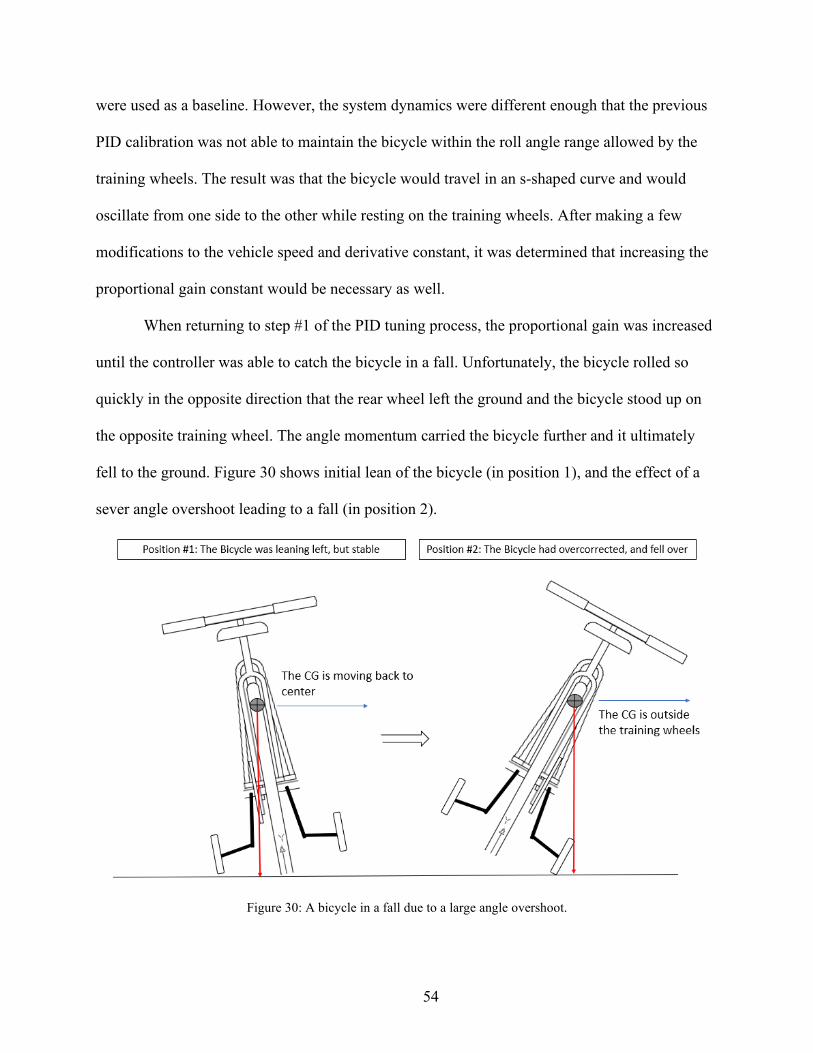
were used as a baseline. However, the system dynamics were different enough that the previous
PID calibration was not able to maintain the bicycle within the roll angle range allowed by the
training wheels. The result was that the bicycle would travel in an s-shaped curve and would
oscillate from one side to the other while resting on the training wheels. After making a few
modifications to the vehicle speed and derivative constant, it was determined that increasing the
proportional gain constant would be necessary as well.
When returning to step #1 of the PID tuning process, the proportional gain was increased
until the controller was able to catch the bicycle in a fall. Unfortunately, the bicycle rolled so
quickly in the opposite direction that the rear wheel left the ground and the bicycle stood up on
the opposite training wheel. The angle momentum carried the bicycle further and it ultimately
fell to the ground. Figure 30 shows initial lean of the bicycle (in position 1), and the effect of a
sever angle overshoot leading to a fall (in position 2).
Figure 30: A bicycle in a fall due to a large angle overshoot.
55
The fall caused significant damage to the support structure on the bicycle, and some of
the wires were torn as well. The wooden mounting post securing the linear actuator to the seat
post had broken off. Also, the battery rack over the rear axle (which holds the motor control, 12V
battery, and 48V battery) broke free as well. The right-side training wheel bracket that the
bicycle had rotated on had also bent under the weight of the bicycle. The wooden mounting
block and some stripped fasteners were replaced, as well as the wires that had been damaged.
The training wheel bracket was also bent back into shape. However, it was noted that even after
the repairs, the rear axle battery rack was not as rigid as it had been before the crash.
Due to concerns with the strength of the rear axle battery rack, and that the training wheel
bracket may yield again under too much weight, testing with the full propulsion system was
postponed (and eventually cancelled due to the COVID pandemic) and plans were made to make
a future upgrade to the prototype bicycle structural design.
Testing did continue with the bicycle system (minus the weight of the 48V battery).
However, in subsequent tests, the bicycle was launched from a running start at various speeds.
4.3 LPV Control Conceptual Demonstration
A third round of tests were performed with the 48V battery removed (to lessen the weight
of the system). The bicycle was launched at two different speeds and the controller response was
observed on a sidewalk and closed road in front of the IAVS building on the University of
Michigan-Dearborn campus.
The objective was to launch the bicycle at a slow-jog and fast-jog and demonstrate a
unique set of PID constants for each speed regime that leads to proper balance control of the
bicycle.
56
The PID tuning process was followed again. A new set of PID constants was generated
for the slow and fast jogging speeds. The controller was able to successfully balance the bicycle
system. Table 8 shows the unique PID gain parameters used in the two sperate speed regimes.
Figure 31 and Figure 32 show the roll angle and measured bicycle speed during the slow and fast
speed trials.
Table 8: PID values for two speed regimes.
Trial #1 Trail #2
Speed regime (m/s) 3.0 – 3.5 3.5 – 4.0
Reference speed Slow jog Fast jog
Proportional gain constant (Kp) 18 13
Derivative gain constant (Kd) 28 20
Integral gain constant (Ki) 0.003 0.003
Shown below is the data recorded during both tests:
Figure 31: Roll angle measurements from lower speed trial.
57
Figure 32: Roll angle measurements from higher speed trial.
Both datasets show that the oscillatory response in the system is not entirely tuned out,
although; the lower speed PID constants do appear to be slightly more refined. It is also
important to note that the initial conditions affect the quality of the test run.
The initial conditions are as follows:
• The launch/release of the bicycle (how the operator released the bicycle)
• The initial steering angle at the time of the launch (which is never perfectly dead ahead)
• The exact orientation of the accelerometer (if it is positioned a few degrees off its
calibrated orientation, measurement error will be present in the data)
Even though the test was performed with a manual launch of the prototype bicycle
system. It was still demonstrated how gain scheduling can be used to change the PID values for
different speed ranges to keep the controller performing as designed. However, future work
should be done to experimentally validate the control laws over a wider speed range.
4.4 Recommendations for Future Prototype Testing
Throughout the testing process several challenges were encountered with setting up each
test run, as well as with the electrical and mechanical hardware. The test planning was also
58
difficult since usually more than one person was required to run the tests. The following
opportunities and recommendations are made for future prototypes and testing:
• A permanent wiring setup. All wiring to and from the Arduino was an on small 22-
gauge wiring connected to and from a breadboard. This worked well for initial signal
identification and for subsystem tests. However, once the entire electrical system was
connected, the high density of wire connections often led to one or more wires been
bumped and losing proper continuity. This resulted in 15-20 minutes of wire inspection
before each batch of testing was performed. It is highly recommended that future testing
be done with at least having the wires soldered into a joint on a breakout board, so that
the connections do not come lose after each day of use.
• Proper electrical component housing. The InvenSense IMU unit was installed directly
on top of the bicycle seat on top of piece of double-sided tape. Although testing was
achievable, great care had to be taken to position the IMU in the exact location both
during the IMU calibration and testing process. More than once it was found that the
bicycle system would unexpectedly performing as was as it had just a few minutes prior.
Many times, it was discovered that the accelerometer was positioned of center, or at an
angle. Also, many other control components were also installed on other unique spots on
the bicycle. It is recommended that a housing box is made for the components. Especially
for the accelerometer, the housing box should have defined locations and features to
properly hold down each motor controller, IMU, battery, and the Arduino.
• Efficient software coding and data logging. As mentioned previously, the software
code for the accelerometer was copied in from a library and little effort was made to
make the system perform more efficiently. The control-loop processing time was about
15ms, which seemed sufficient for interacting with the IMU and controlling the traction
motor and linear actuator. However, once a data recording device (an SD card with a chip
reader) was connected to the Arduino as well, the processing time dropped substantially,
and it took an additional 0.5-0.75 seconds for each iteration of the stability code. The
Arduino was programmed to completely shut down communications on each control
iteration. Thus, each time the Arduino needed to write data to the SD card, it had to re-
initialize communications with the SD card reader. The data write time slowed down the
59
system too much and the microcontroller was no longer able to iterate fast enough to
stabilize the roll of the bicycle. Therefore, the roll angle and velocity data of the bicycle
was captured with an iPhone 7 that was strapped to the bicycle during the test. The
overall code structure of the controller should be evaluated. Any unnecessary functions or
commands should be removed. Also, the SD card reader should be initialized at the very
beginning of the test and stay linked to the Arduino throughout the test to enable fast and
efficient data logging.
• Higher performing electrical hardware and measurement equipment. One of the
objectives of this research was to maintain a small budget and develop a low-cost
stability control system, if possible. While the team achieved this goal with the hardware
and sensors selected, investing in something more than an entry-level microcontroller and
IMU could yield higher performance and a more robust control solution. It would also
provide the processing power to handle more complex control algorithms and handle
auxiliary assignments that may be needed if the bicycle stability and propulsion system is
integrated into a full autonomous vehicle control platform.
• Dedicated test surfaces. It was beneficial to have more than one person present when
testing so that someone could set up the cameras and record observations while the other
person launched the bicycle. Coordinating schedules was compounded by not have a
dedicated test space. Sometimes it was difficult to find a smooth road or sidewalk surface
where the traffic was low enough to be able to perform testing. During one test morning,
the wider sidewalk and service road were close for resurfacing, and we were forced to run
tests in the parking lot. The uneven nature of the asphalt and small cracks and holes made
it difficult to know if the stability challenges were due to the controller or due to noise
input from the road surface. If a dedicated test surface were available, it would make the
testing time more efficient and controlled.
Besides the general recommendations listed above, the current prototype bicycle should
be reinforced (possibly replaced by a manufactured e-bike) so that trials may continue with a
functional propulsion system. A key next step would be to trial the control laws across a wider
speed range. It would also be possible to test the control theory through CAE before more
60
experimental testing is performed. Although LPV control appears viable at this time, there are
also a wide variety of other, more complex, control methods that may achieve similar, or
improved, results.
61
Chapter 5 Conclusions and Considerations for Future Work
In this paper, I reported on the design evolution of the bicycle and other single-track
systems and how they have become a key tool for people and goods transportation worldwide.
The form factor, carrying capacity, maneuverability, and cost of single-track vehicles makes
them advantageous in a variety of circumstances and justifies their use case in the 21st Century.
As autonomous double-track vehicles arrive on public roads, it is natural that single-track
autonomous systems will also be considered. Many of the functions of autonomous systems for
automobiles can be directly applied to an inline wheel system as well. The unique challenge lies
in the dynamics of the single-track vehicle.
The inherent instability and non-minimum phase dynamics of single-track vehicles poses
a challenge from a controls perspective and has intrigued scientists and engineers for over a
century. Although many researchers have provided commentary on the stability and tracking
control of a riderless bicycle, relatively few bodies of work have validated their analysis through
experimental testing. When a human rides on a bicycle, they learn to intuitively use a
combination of lean and steering actuation to conduct the bicycle in a stable manner. The issue
becomes more complicated when the rider is removed. Using solely steering or lean control
comes has tradeoffs in maneuverability and each proves unreliable in certain scenarios (for
example, steering actuation when the bicycle is at rest). Constructing an integrated controller has
its own set of challenges as well.
62
Future applications of this research can expand beyond bicycle stability analysis. The
stability methods here apply equally to motorcycles, mopeds, scooters, and other inline wheel
systems. The µSMET project at the University of Michigan – Dearborn is another vehicle where
single-track stability method described in this thesis can apply. The vehicle is a tricycle hybrid
which can adjust the distance between its rear wheel axles. In its narrow configuration, the
vehicle will behave much more like a single-track vehicle rather than a tricycle. Figure 33 shows
the µSMET in its narrow and expanded configuration. The same control law used in this thesis
would be a good starting point for active roll stabilization of the µSMET [62].
Figure 33: µSMET shown in its narrow (left) and expanded configuration (right).
In this thesis, we have successfully demonstrated that, through gain scheduling, a PID-
type controller can achieve the self-balancing of an autonomous single-track vehicle by using a
linear actuator to implement front-fork steering control. This control method is novel in the way
in which the front fork is actuated. To the best of my knowledge, no other body of research
outlines such use of a linear actuator. The manual PID tuning process outlined in this body of
work is also unique, as well as the specifics of the control law (although others have used PID
controllers).
The Linear-Parameter Varying gain scheduling approach has been shown to be successful
at maintaining a single-track vehicle upright. Much work needs to be done to determine the path-
63
tracking capability of such a method. Some future research could include experimental validation
of the controller across a wider speed range, trialing maintaining a bicycle in a steady-state turn,
developing an accurate model of the full system so that less experimental testing is required, and
exploring more advanced control methods.
64
Appendices
65
Appendix A Modeling Mass, Center of Gravity, and Inertia
The following appendix outlines how the bicycle system mass moment of inertia was
calculated.
Assumptions:
• Assume all electronics components added to the bicycle are sufficiently small that
their inertia may be modeled individually as a point mass, with the center of
gravity at the center of the object.
• Additional components added to the bicycle may also be modeled as a point mass.
• The bicycle will be modeled as a rectangular plane (except for the powered
wheel). The power wheel is considered a significant enough weight to be modeled
separately as a point mass.
• The height of the center of gravity of the bicycle is approximately 70 percent of
the height of the bicycle.
Process for finding the bicycle’s center of gravity (ground plane projection):
• Measure the bicycle wheelbase.
• Measure the total weight of the bicycle.
• Measure the proportion of weight on each bicycle tire.
• Create a free-body diagram and a moment-balance equation to determine the CG
location relative to the bicycle front and rear axles.
66
Process for calculating inertia:
• Each component of the bicycle was individually weighed.
• The height of each component (when installed) above the ground plane was
measured.
• The standard engineering formula for the mass moment of inertia for point masses
and beams was used to model the inertia of each system and the parallel axis
theorem was used to calculate the mass moment of inertia about the ground plane
[63], [64].
• Sum the mass and inertia of the bicycle and all the components.
67
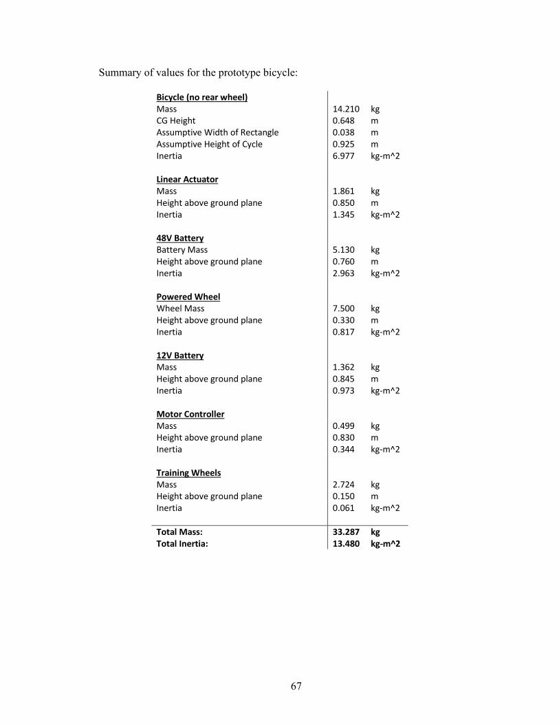
Summary of values for the prototype bicycle:
Bicycle (no rear wheel) Mass 14.210 kg CG Height 0.648 m Assumptive Width of Rectangle 0.038 m Assumptive Height of Cycle 0.925 m Inertia 6.977 kg-m^2 Linear Actuator Mass 1.861 kg Height above ground plane 0.850 m Inertia 1.345 kg-m^2 48V Battery Battery Mass 5.130 kg Height above ground plane 0.760 m Inertia 2.963 kg-m^2 Powered Wheel Wheel Mass 7.500 kg Height above ground plane 0.330 m Inertia 0.817 kg-m^2 12V Battery Mass 1.362 kg Height above ground plane 0.845 m Inertia 0.973 kg-m^2 Motor Controller Mass 0.499 kg Height above ground plane 0.830 m Inertia 0.344 kg-m^2 Training Wheels Mass 2.724 kg Height above ground plane 0.150 m Inertia 0.061 kg-m^2 Total Mass: 33.287 kg Total Inertia: 13.480 kg-m^2
68
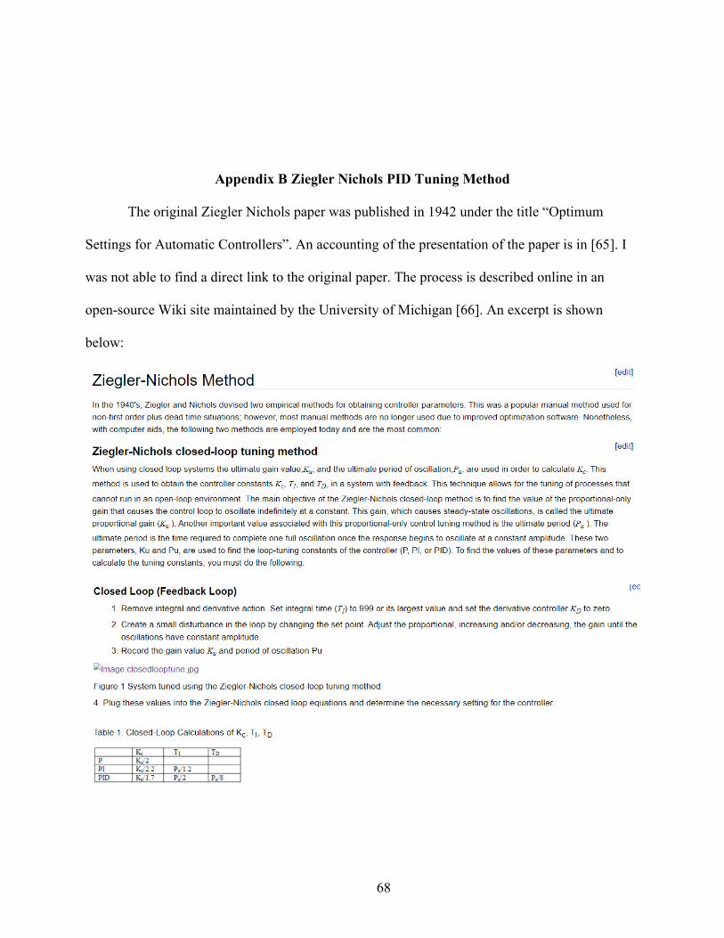
Appendix B Ziegler Nichols PID Tuning Method
The original Ziegler Nichols paper was published in 1942 under the title “Optimum
Settings for Automatic Controllers”. An accounting of the presentation of the paper is in [65]. I
was not able to find a direct link to the original paper. The process is described online in an
open-source Wiki site maintained by the University of Michigan [66]. An excerpt is shown
below:
69
References
[1] E. Salmeron-Manzano and F. Manzano-Agugliaro, “The Electric Bicycle: Worldwide Research Trends,” Energies, vol. 11, 2018, doi: 10.3390/en11071894.
[2] Z. Liu, L. Ma, T. Huang, and H. Tang, “Collaborative Governance for Responsible Innovation in the Context of Sharing Economy: Studies on the Shared Bicycle Sector in China,” J. Open Innov. Technol. Mark. Complex. Artic., vol. 6, 2020, doi: 10.3390/joitmc6020035.
[4] “Italian bicycle sales ‘surpass those of cars’ - BBC News,” BBC News, 2012. https://www.bbc.com/news/world-europe-19801599 (accessed Jun. 20, 2021).
[8] “Rover ‘Safety’ bicycle, 1885 | Science Museum Group Collection.” https://collection.sciencemuseumgroup.org.uk/objects/co25833/rover-safety-bicycle-1885-bicycle (accessed May 14, 2020).
[9] “Sun Bicycles Skylar 5 - Bicycle Renaissance Bike Shop in New York City on the Upper West Side.” https://www.bicyclerenaissance.com/product/sun-bicycles-skylar-5-263384-1.htm (accessed May 14, 2020).
[10] T. Hadland, Bicycle Design: An Illustrated History. Cambridge: MIT Press Books, 2014.
[12] K. J. Astrom, R. E. Klein, and A. Lennartsson, “Bicycle Dynamics and Control: Adapted bicycles for education and research,” IEEE Control Syst., vol. 25, no. 4, pp. 26–47, 2005, doi: 10.1109/MCS.2005.1499389.
[13] S. Pendleton et al., “Multi-class driverless vehicle cooperation for mobility-on-demand,” 21st World Congr. Intell. Transp. Syst. ITSWC 2014 Reinventing Transp. Our Connect. World, no. September 2016, 2014.
[14] S. Behere and M. Törngren, “A functional reference architecture for autonomous driving,” Inf. Softw. Technol., vol. 73, pp. 136–150, 2016, doi: 10.1016/j.infsof.2015.12.008.
[15] A. Nardi and A. Armato, “Functional safety methodologies for automotive applications,” IEEE/ACM Int. Conf. Comput. Des. Dig. Tech. Pap. ICCAD, vol. 2017-Novem, pp. 970–975, 2017, doi: 10.1109/ICCAD.2017.8203886.
[16] Y. Jung, S. Park, and M. Han, “Automotive Hardware Development According to ISO 26262,” 13th Int. Conf. Adv. Commun. Technol., pp. 588–592, 2011.
[17] M. Nagai, “Analysis of Rider and Single-track-vehicle System,” Automatica, vol. 19, no. 6, pp. 737–740, 1983.
[18] J. D. G. Kooijman and A. L. Schwab, “A review on bicycle and motorcycle rider control with a perspective on handling qualities,” Veh. Syst. Dyn., vol. 51, no. 11, pp. 1722–1764, 2013, doi: 10.1080/00423114.2013.824990.
[19] S. Miyagishi, I. Kageyama, K. Takama, M. Baba, and H. Uchiyama, “Study on construction of a rider robot for two-wheeled vehicle,” JSAE Rev., vol. 24, no. 3, pp. 321–326, 2003, doi: 10.1016/S0389-4304(03)00045-6.
[20] A. L. Schwab and J. P. Meijaard, “A review on bicycle dynamics and rider control,” Veh. Syst. Dyn., vol. 51, no. 7, pp. 1059–1090, 2013, doi: 10.1080/00423114.2013.793365.
[21] T. Saguchi, K. Yoshida, and M. Takahashi, “Stable running control of autonomous bicycle robot,” Nihon Kikai Gakkai Ronbunshu, C Hen/Transactions Japan Soc. Mech. Eng. Part C, vol. 73, no. 7, pp. 2036–2041, 2007, doi: 10.1299/kikaic.73.2036.
[22] B. Michini and S. Torrez, “Autonomous Stability Control of a Moving Bicycle,” Am. Inst. Aeronaut. Astronaut., pp. 1–10, 2006.
[23] J. F. Lenkeit, “A servo rider for the automatic and remote path control of a motorcycle,” SAE Tech. Pap., 1995, doi: 10.4271/950199.
[24] Z. Fawaz, R. Smith, P. Muench, S. Lakshmanan, and A. Mohammadi, “Design and
benchtop validation of an autonomous bicycle with linear electric actuators,” p. 11, 2019, doi: 10.1117/12.2519189.
71
[25] M. Yamakita and A. Utano, “Automatic Control of Bicycles with a Balancer,” in IEEE/ASME International Conference on Advanced Intelligent Mechatronics, 2005, pp. 24–28.
[26] L. Keo and M. Yamakita, “Controller Design of an Autonomous Bicycle with Both Steering and Balancer Controls,” in 18th IEEE International Conference on Control Applications, 2009, pp. 1294–1299.
[27] V. Cerone, D. Andreo, M. Larsson, and D. Regruto, “Stabilization of a Riderless Bicycle: A Linear-Parameter-Varying Approach,” IEEE Control Syst., vol. 30, no. 5, pp. 23–32, 2010, doi: 10.1109/MCS.2010.937745.
[28] D. Andreo, V. Cerone, D. Dzung, and D. Regruto, “Experimental results on LPV stabilization of a riderless bicycle,” Proc. Am. Control Conf., pp. 3124–3129, 2009, doi: 10.1109/ACC.2009.5160397.
[29] I. I. Boldea and S. A. Nasar, “Linear electric actuators and generators,” IEEE Trans. Energy Convers., vol. 14, no. 3, pp. 712–717, 1999, doi: 10.1109/60.790940.
[30] B. Na, H. Choi, and K. Kong, “Design of a Direct-Driven Linear Actuator,” IEEE/ASME Trans. Mechatronics, vol. 20, no. 99, pp. 1–10, 2014, doi: 10.1109/TMECH.2014.2326696.
[31] M. Bergamasco, F. Salsedo, and P. Dario, “Linear SMA Motor as Direct-Drive Robotic Actuator,” in 1989 International Conference on Robotics and Automation, 1989, pp. 618–623, doi: 10.1109/ROBOT.1989.100053.
[32] F. Sup, A. Bohara, and M. Goldfarb, “Design and control of a powered transfemoral prosthesis,” Int. J. Rob. Res., vol. 27, no. 2, pp. 263–273, 2008, doi: 10.1177/0278364907084588.
[33] B. Na, H. Choi, and K. Kong, “Design of a Direct-Driven Linear Actuator for a High-Speed Quadruped Robot, Cheetaroid-I,” IEEE/ASME Trans. Mechatronics, vol. 20, no. 99, pp. 1–10, 2014.
[34] P. Lucidarme, N. Delanoue, F. Mercier, Y. Aoustin, C. Chevallereau, and P. Wenger, “Preliminary Survey of Backdrivable Linear Actuators for Humanoid Robots,” CISM Int. Cent. Mech. Sci. Courses Lect., vol. 584, no. February, pp. 304–313, 2019, doi: 10.1007/978-3-319-78963-7_39.
[35] J. Hollerbach, I. Hunter, and J. Ballantyne, “A Comparative Analysis of Actuator Technologies for Robotics,” in The Robotics Review 2, MIT Press, 1992, pp. 299–342.
[36] T. Ishida and A. Takanishi, “A Robot Actuator Development With High Backdrivability,” in 2006 IEEE Conference on Robotics, Automation and Mechatronics, Jun. 2006, pp. 1–6, doi: 10.1109/RAMECH.2006.252631.
72
[37] P. M. Wensing, A. Wang, S. Seok, D. Otten, J. Lang, and S. Kim, “Proprioceptive Actuator Design in the MIT Cheetah: Impact Mitigation and High-Bandwidth Physical Interaction for Dynamic Legged Robots,” IEEE Trans. Robot., vol. 33, no. 3, pp. 509–522, Jun. 2017, doi: 10.1109/TRO.2016.2640183.
[38] “SUV(HATCHBACK) Soft Close Automatic Door Suction | Changyi.” http://changyi-china.com.cn/product/automatic-tailgate-lift-for-suv-electric-suction/ (accessed Apr. 08, 2021).
[39] “2013-2019 Ford Flex Actuator DA8Z-14B351-A | Ford Discount Parts,” Ford Discount Parts. https://www.forddiscountparts.com/oem-parts/ford-actuator-da8z14b351a?origin=pla&gclid=CjwKCAjw07qDBhBxEiwA6pPbHnfqR738Oxrm93h2sVUNYYI68GmP6INk4GajI_8Gq2Awk77cVZo8oBoC93YQAvD_BwE (accessed Apr. 08, 2021).
[40] Z. Fawaz, R. Smith, P. Muench, S. Lakshmanan, and A. Mohammadi, “Design and benchtop validation of an autonomous bicycle with linear electric actuators,” in Proceedings of SPIE - The International Society for Optical Engineering, 2019, vol. 11021, doi: 10.1117/12.2519189.
[41] T. Newcombe, “Amid Cycling Surge, Sport Of Mountain Biking Is Seeing Increased Sales And Trail Usage,” Forbes Magazine, 2020. https://www.forbes.com/sites/timnewcomb/2020/07/13/amidst-cycling-surge-sport-of-mountain-biking-seeing-increased-sales-trail-usage/?sh=53ce6e423ddf (accessed Apr. 03, 2021).
[42] B. Beacham, “5 Best Electric Bikes - Apr. 2021 - BestReviews,” Daily News, 2021. https://reviews.nydailynews.com/reviews/best-electric-bikes (accessed Apr. 03, 2021).
[44] R. P. B. H. Center, “Riding Rad with Regenerative Braking,” Rad Power Bikes, 2021. https://radpowerbikes.zendesk.com/hc/en-us/articles/360045171734-Riding-Rad-with-Regenerative-Braking (accessed Apr. 03, 2021).
[45] “48V 1000W Front Wheel E-Bike Motor Conversion Kit,” Jaxpety.com. https://www.jaxpety.com/bicycle-motor-kit-48v-1000w-rear-wheel-electric-conversion.html.
[46] “MPC 3620 Heavy Duty Linear Actuator, 12V DC, 10" Stroke, 770 lb. Max Load, Black Finish: Amazon.com: Automotive.” https://www.amazon.com/MPC-3620-Linear-Actuator-Stroke/dp/B012YAYGVC (accessed Nov. 28, 2020).
73
[47] “MPC LAD-HS10 High Speed Linear Actuator with 10" Stroke, Heavy 12V, 65 mm/seconds Speed: Amazon.com: Automotive.” https://www.amazon.com/MPC-LAD-HS10-Linear-Actuator-seconds/dp/B00JYOIZ64/ref=cm_cr_arp_d_product_top?ie=UTF8 (accessed Nov. 28, 2020).
[48] “Arduino Uno Webpage.” https://store.arduino.cc/usa/arduino-uno-rev3 (accessed May 12, 2020).
[49] Martin Marino, “Arduino vs Microprocessor vs Microcontroller,” StackExchange - Electronics, 2014. https://electronics.stackexchange.com/questions/99434/arduino-vs-microprocessor-vs-microcontroller (accessed May 12, 2020).
[50] InvenSense, “MPU-6050 Product Specification Revision 3.4.” pp. 1–11, 2013.
[54] M. Carvallo, “Theorie De Mouvement Du Monocycle Et De La Bycyclette.” Gauthier-Villars, Paris, 1901, [Online]. Available: http://scholar.google.com/scholar?hl=en&btnG=Search&q=intitle:Theorie+du+mouvement+du+Monocycle+et+de+la+Bicyclette#0.
[55] T. Tun, L. Rothenbusch, P. Ingenlath, A. Brezing, and B. Corves, “Modelling , Implementation and Analysis of the Carvallo-Whipple Bicycle Model in Msc Adams,” in IASTEM International Conference, 2018, no. August, pp. 19–23, doi: 10.13140/RG.2.2.22633.75369.
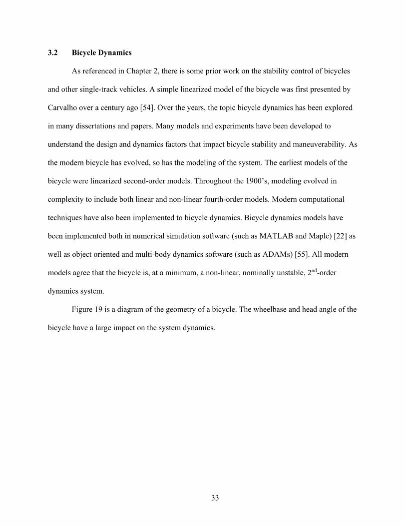
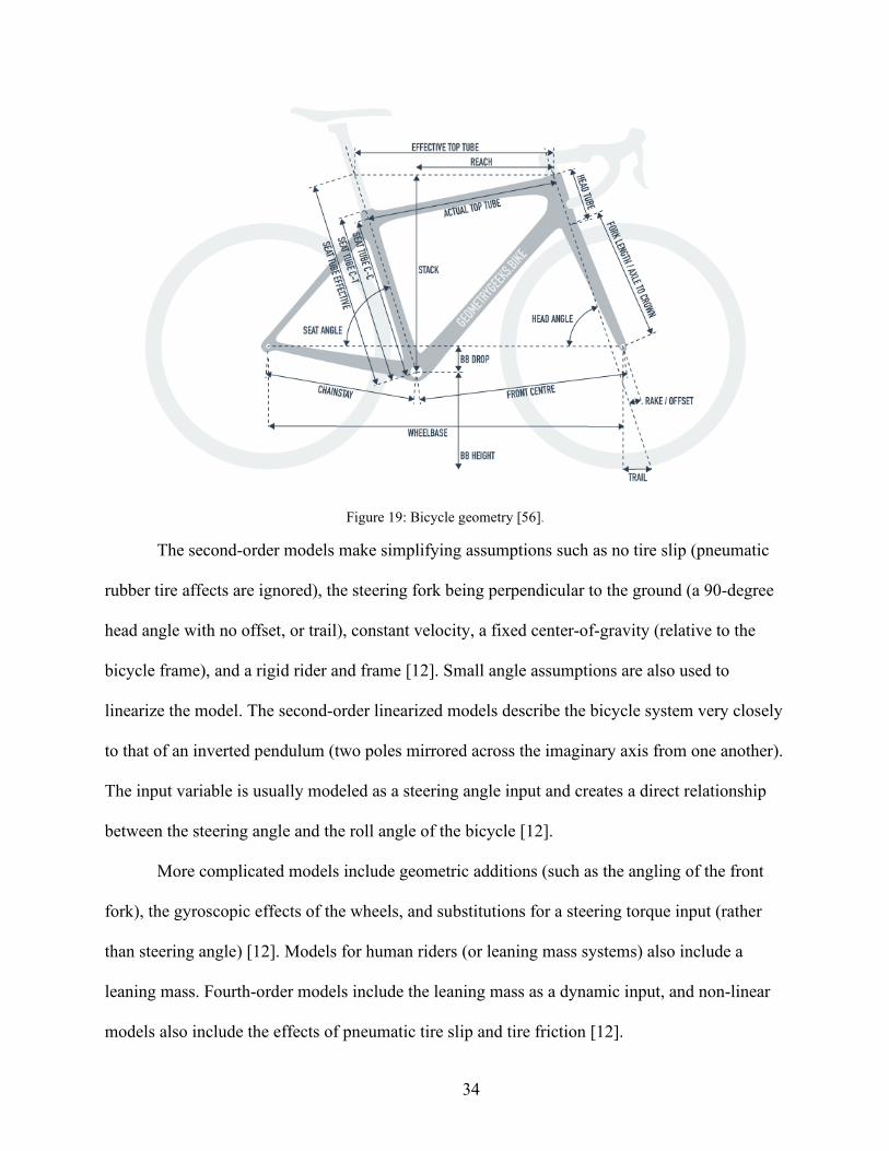
[56] “Understanding Bike Geometry,” GeometryGreeks.BIKE. https://geometrygeeks.bike/understanding-bike-geometry (accessed Jun. 20, 2021).
[57] D. Karnopp, Vehicle Dynamics, Stability, and Control, 2nd ed. Boca Raton: CRC Press, 2013.
[58] K. J. Åström and T. Hägglund, “Revisiting the Ziegler-Nichols step response method for PID control,” J. Process Control, vol. 14, no. 6, pp. 635–650, 2004, doi: https://doi.org/10.1016/j.jprocont.2004.01.002.
[59] V. Bobál, J. Macháček, and R. Prokop, “Tuning of Digital PID Controllers Based on Ziegler - Nichols Method,” IFAC Proceedings Volumes, vol. 30, no. 21. pp. 145–150, 1997, doi: 10.1016/s1474-6670(17)41430-3.
74
[60] R. Sen, C. Pati, S. Dutta, and R. Sen, “Comparison Between Three Tuning Methods of PID Control for High Precision Positioning Stage,” MAPAN, vol. 30, no. 1, pp. 65–70, 2015, doi: 10.1007/s12647-014-0123-z.
[61] Felix, “control - What are good strategies for tuning PID loops? - Robotics Stack
[62] C. Adam, T. Kleinow, K. Grenn, B. Mason, O. Sapunkov, and P. Muench, “µSMET : A Lightweight Transport Robot,” in SPIE Defense + Commercial Sensing, 2021, vol. 11758, no. 1175807.
[63] “Mass Moment of Inertia Equations | Engineers Edge | www.engineersedge.com.” https://www.engineersedge.com/mechanics_machines/mass_moment_of_inertia_equations_13091.htm (accessed Jun. 21, 2021).
[65] J. G. Ziegler and N. B. Nichols, “Optimum Settings for Automatic Controllers,” J. Dyn. Syst. Meas. Control, vol. 115, no. 2B, pp. 220–222, Jun. 1993, doi: 10.1115/1.2899060.