1 A Linear-Programming Approximation of AC Power Flows Carleton Coffrin, Member, IEEE, Pascal Van Hentenryck, Member, IEEE Abstract—Linear active-power-only DC power flow approx- imations are pervasive in the planning and control of power systems. However, these approximations fail to capture reactive power and voltage magnitudes, both of which are necessary in many applications to ensure voltage stability and AC power flow feasibility. This paper proposes linear-programming models (the LPAC models) that incorporate reactive power and voltage magnitudes in a linear power flow approximation. The LPAC models are built on a convex approximation of the cosine terms in the AC equations, as well as Taylor approximations of the remaining nonlinear terms. Experimental comparisons with AC solutions on a variety of standard IEEE and MATPOWER benchmarks show that the LPAC models produce accurate values for active and reactive power, phase angles, and voltage magnitudes. The potential benefits of the LPAC models are illustrated on two “proof-of-concept” studies in power restoration and capacitor placement. Index Terms—DC power flow, AC power flow, LP power flow, linear relaxation, power system analysis, capacitor placement, power system restoration NOMENCLATURE e I AC Current e V = v + iθ AC voltage e S = p + iq AC power e Z = r + ix Line impedance e Y = g + ib Line admittance e Y b = g y + ib y Y-Bus element e Y c = g c + ib c Line charge e Y s = g s + ib s Bus shunt e T = t + is Transformer parameters e V = | e V |∠θ ◦ Polar form e S n AC Power at bus n e S nm AC Power on a line from n to m PN Power network N Set of buses in a power network L Set of lines in a power network G Set of voltage controlled buses s Slack Bus | e V h | Hot-Start voltage magnitude | e V t | Target voltage magnitude φ Voltage magnitude change Δ Absolute difference δ Percent difference ˆ x Approximation of x x Upper bound of x x Lower bound of x C. Coffrin and P. Van Hentenryck are members of the Optimization Research Group, NICTA, Victoria 3010, Australia. P. Van Hentenryck is Professor in the School of Engineering at the University of Melbourne. I. I NTRODUCTION O PTIMIZATION technology is widely used in modern power systems [1] and has resulted in millions of dollars in savings annually [2]. But the increasing role of demand response, the integration of renewable sources of energy, and the desire for more automation in fault detection and recovery pose new challenges for the planning and control of electrical power systems [3]. Power grids now need to operate in more stochastic environments and under varying operating conditions, while still ensuring system reliability and security. Optimization of power systems encompasses a broad spec- trum of problem domains, including optimal power flow [4], [5], [6], [7], [8], [9], [10], [11], [12], [13], [14], LMP-base market calculations [15], [16], [17], transmission switching [18], [19], [20], real-time security-constrained dispatch [21], [22], day-ahead security-constrained unit commitment [23], [24], [25], distribution network configuration [26], [27], capac- itor placement [28], [29], [30], expansion planning [31], [32], [33], [34], [35], [36], [37], [38], [39], vulnerability analysis [40], [41], [42], [43], [44], and power system restoration [45], [46] to name a few. Some of these use active power only, while others consider both active and reactive power. Restricting attention to active power is often appealing computationally as the nonlinear AC power flow equations can then be approximated by a set of linear equations that define the so-called Linearized DC (LDC) model. Under normal operating conditions and with some adjustment for line losses, the LDC model produces a reasonably accurate approximation of the AC power flow equations for active power [47]. Moreover, the LDC model can be embedded in Mixed-Integer Programming (MIP) models for a variety of optimization applications in power system operations. This is particularly attractive as the computational efficiency of Linear Programming (LP) and MIP solvers has significantly improved over the last two decades [48]. However, the LDC model does not capture reactive power and hence cannot be used for applications such as capacitor placement and voltage stability to name only two. Moreover, the accuracy of the LDC model outside normal operating conditions is an open point of discussion (e.g., [15], [47], [49], [50], [51]). This in turn raises concerns for other applications such transmission planning, vulnerability analysis, and power restoration, which may return infeasible or suboptimal solu- tions when the LDC model is used to approximate the AC power flow equations. As a result, these applications often turn to nonlinear programming techniques [8], [13], [14], [17], iterative heuristics and decomposition [11], [12], [36], arXiv:1206.3614v3 [cs.AI] 6 Aug 2013
Transcript
1
A Linear-Programming Approximation ofAC Power Flows
Carleton Coffrin, Member, IEEE, Pascal Van Hentenryck, Member, IEEE
Abstract—Linear active-power-only DC power flow approx-imations are pervasive in the planning and control of powersystems. However, these approximations fail to capture reactivepower and voltage magnitudes, both of which are necessary inmany applications to ensure voltage stability and AC powerflow feasibility. This paper proposes linear-programming models(the LPAC models) that incorporate reactive power and voltagemagnitudes in a linear power flow approximation. The LPACmodels are built on a convex approximation of the cosine termsin the AC equations, as well as Taylor approximations of theremaining nonlinear terms. Experimental comparisons with ACsolutions on a variety of standard IEEE and MATPOWERbenchmarks show that the LPAC models produce accuratevalues for active and reactive power, phase angles, and voltagemagnitudes. The potential benefits of the LPAC models areillustrated on two “proof-of-concept” studies in power restorationand capacitor placement.
Index Terms—DC power flow, AC power flow, LP power flow,linear relaxation, power system analysis, capacitor placement,power system restoration
NOMENCLATURE
I AC CurrentV = v + iθ AC voltageS = p+ iq AC powerZ = r + ix Line impedanceY = g + ib Line admittanceY b = gy + iby Y-Bus elementY c = gc + ibc Line chargeY s = gs + ibs Bus shuntT = t+ is Transformer parametersV = |V |∠θ◦ Polar form
Sn AC Power at bus nSnm AC Power on a line from n to mPN Power networkN Set of buses in a power networkL Set of lines in a power networkG Set of voltage controlled busess Slack Bus|V h| Hot-Start voltage magnitude|V t| Target voltage magnitudeφ Voltage magnitude change∆ Absolute differenceδ Percent differencex Approximation of xx Upper bound of xx Lower bound of x
C. Coffrin and P. Van Hentenryck are members of the OptimizationResearch Group, NICTA, Victoria 3010, Australia. P. Van Hentenryck isProfessor in the School of Engineering at the University of Melbourne.
I. INTRODUCTION
OPTIMIZATION technology is widely used in modernpower systems [1] and has resulted in millions of dollars
in savings annually [2]. But the increasing role of demandresponse, the integration of renewable sources of energy,and the desire for more automation in fault detection andrecovery pose new challenges for the planning and control ofelectrical power systems [3]. Power grids now need to operatein more stochastic environments and under varying operatingconditions, while still ensuring system reliability and security.
Optimization of power systems encompasses a broad spec-trum of problem domains, including optimal power flow [4],[5], [6], [7], [8], [9], [10], [11], [12], [13], [14], LMP-basemarket calculations [15], [16], [17], transmission switching[18], [19], [20], real-time security-constrained dispatch [21],[22], day-ahead security-constrained unit commitment [23],[24], [25], distribution network configuration [26], [27], capac-itor placement [28], [29], [30], expansion planning [31], [32],[33], [34], [35], [36], [37], [38], [39], vulnerability analysis[40], [41], [42], [43], [44], and power system restoration [45],[46] to name a few. Some of these use active power only,while others consider both active and reactive power.
Restricting attention to active power is often appealingcomputationally as the nonlinear AC power flow equationscan then be approximated by a set of linear equations thatdefine the so-called Linearized DC (LDC) model. Undernormal operating conditions and with some adjustment forline losses, the LDC model produces a reasonably accurateapproximation of the AC power flow equations for activepower [47]. Moreover, the LDC model can be embedded inMixed-Integer Programming (MIP) models for a variety ofoptimization applications in power system operations. This isparticularly attractive as the computational efficiency of LinearProgramming (LP) and MIP solvers has significantly improvedover the last two decades [48].
However, the LDC model does not capture reactive powerand hence cannot be used for applications such as capacitorplacement and voltage stability to name only two. Moreover,the accuracy of the LDC model outside normal operatingconditions is an open point of discussion (e.g., [15], [47], [49],[50], [51]). This in turn raises concerns for other applicationssuch transmission planning, vulnerability analysis, and powerrestoration, which may return infeasible or suboptimal solu-tions when the LDC model is used to approximate the ACpower flow equations. As a result, these applications oftenturn to nonlinear programming techniques [8], [13], [14],[17], iterative heuristics and decomposition [11], [12], [36],
arX
iv:1
206.
3614
v3 [
cs.A
I] 6
Aug
201
3
2
[42], model relaxation [7], [28], tabu search [30], and geneticalgorithms [29], [34] to ensure feasibility. These techniquesoften require extensive tuning for each problem domain,may consume significant computational resources, and cannotguarantee global optimality.
This paper aims at bridging the gap between the LDC modeland the AC power flow equations. It presents linear programsto approximate the AC power flow equations. These linearprograms, called the LPAC models, are based on two ideas:
1) They reason both on the voltage phase angles and thevoltage magnitudes, which are coupled through equa-tions for active and reactive power;
2) They use a piecewise linear approximation of the cosineterm in the power flow equations and Taylor series forapproximating the remaining nonlinear terms.
The LPAC models have been evaluated experimentally overa number of standard benchmarks under normal operatingconditions and various contingencies. Experimental compar-isons with AC solutions on standard IEEE and MatPowerbenchmarks shows that the LPAC models are highly accuratefor active and reactive power, phase angles, and voltage mag-nitudes. Moreover, the LPAC models can be integrated in MIPmodels for applications reasoning about reactive power (e.g.,capacitor placement) or topological changes (e.g., transmissionplanning, vulnerability analysis, and power restoration).
This rest of this paper presents a rigorous and systematicderivation of the LPAC models, experimental results abouttheir accuracy, and its application to power restoration andcapacitor placement. Section II reviews the AC power flowequations. Section III derives the LPAC models and SectionIV presents the experimental results on its accuracy. Sec-tion V presents the “proof-of-concept” experiments in powerrestoration and capacitor placement to demonstrate potentialapplications of the LPAC models. Section VI discusses relatedwork and Section VII concludes the paper.
II. REVIEW OF AC POWER FLOW
The steady state AC power for bus n is given by
Sn =
n 6=m∑m
VnV∗n Y∗nm − VnV ∗mY ∗nm. (1)
This equation is not symmetric. From the perspective of busn, the power flow on a line to bus n is
VnV∗n Y∗nm − VnV ∗mY ∗nm
while, from the perspective of bus m, it is
VmV∗mY∗mn − VmV ∗n Y ∗mn.
In general, Snm 6= Smn.
A. The Traditional Representation
The AC power flow definition is typically expanded in termsof real numbers only. By representing power in rectangular
form, the real (pn) and imaginary (qn) terms become
The Y-Bus Matrix: The formulation can be simplified furtherby using a Y-Bus Matrix, i.e., a precomputed lookup tablethat allows the power flow at each bus to be written as asummation of 2n terms instead a summation of 3(n−1) terms.Observe that, in the power flow equations (1), the first termVnV
∗n Y∗nm is a special case of the second term −VnV ∗mY ∗nm
with −Vm = Vn. We can eliminate this special case by
1) extending the summation to include n terms, i.e.,∑n 6=m
m
becomes∑
m;2) defining the Y-Bus admittance Y b
nm as
Y bnn =
n6=m∑m
Ynm
Y bnm =−Ynm
Given the Y-Bus, the power flow equations (1) can be rewrittenas a single summation
Sn =∑m
VnV∗mY
bnm (2)
giving us the popular formulation of active and reactive power:
pn =∑m
|Vn||Vm|(gynm cos(θ◦n−θ◦m)+bynm sin(θ◦n−θ◦m)) (3)
qn =∑m
|Vn||Vm|(gynm sin(θ◦n−θ◦m)−bynm cos(θ◦n−θ◦m)) (4)
B. An Alternate Representation
The Y-Bus formulation is concise but makes it difficult toreason about the power flow equations. This paper uses themore explicit equations which can be presented as bus andline equations as follows:
pn =
n 6=m∑m
pnm (5)
qn =
n 6=m∑m
qnm (6)
pnm = |Vn|2gnm − |Vn||Vm|gnm cos(θ◦n − θ◦m)
−|Vn||Vm|bnm sin(θ◦n − θ◦m) (7)
qnm =−|Vn|2bnm + |Vn||Vm|bnm cos(θ◦n − θ◦m)
−|Vn||Vm|gnm sin(θ◦n − θ◦m) (8)
Once again, 7 and 8 are asymmetric and the line admittancevalues Y have not been modified.
3
C. Extensions for Practical Power Networks
In the above derivation, each line is a conductor with animpedance Z. The formulation can be extended to line charg-ing and other components such as transformers and bus shunts,which are present in nearly all AC system benchmarks. Weshow how to model these extensions in the Y-Bus formulationfor simplicity.
Line Charging: A line connecting buses n and m mayhave a predefined line charge Y c. Steady state AC modelstypically assume that a line charge is evenly distributed acrossthe line and hence it is resonable to assign equal portions ofits charge to both sides of the line. This is incorporated in theY-Bus matrix as follows:
Y b′
nn = Y bnn + Y c
nm/2,
Y b′
mm = Y bmm + Y c
nm/2.
Transformers: A transformer connecting bus n to busm can be modeled as a line with modifications to the Y-Busmatrix. The properties of the transformer are captured by acomplex number Tnm = |T |∠s◦, where |T | is the tap ratiofrom n to m and s◦ is the phase shift. It is worth notingthat the direction of a transformer-line is very important tomodel the tap ratio and phase shift properly. A transformer ismodeled in the Y-Bus matrix as follows:
Y b′
nn = Y bnn − Ynm + Ynm/|Tnm|2,
Y b′
nm = Ynm/T∗nm,
Y b′
mn = Ymn/Tnm.
If a line charge exists, it must be applied before the transformercalculation, i.e.,
Y b′
nn = Y bnn − Ynm + (Ynm + Y c
nm/2)/|Tnm|2
Bus Shunts: A bus n may have a shunt element which ismodeled as a fixed admittance to ground with a value of Y s.In the Y-Bus matrix, we have
Y b′
nn = Y bnn + Y s
n
Unlike line charging, this extension is not affected by trans-formers, since it applies to a bus and not a line.
D. The Linearized DC Power Flow
Many variants of the Linearized DC (LDC) model exist[52], [53], [54], [55]. A comprehensive review of all thesevariants is outside the scope of this work but an in-depthdiscussion can be found in [47]. For brevity, we only reviewthe simplest and most popular variant of the LDC, which isderived from the AC equations through a series of approxi-mations justified by operational considerations under normaloperating conditions. In particular, the LDC assumes that (1)the susceptance is large relative to the conductance |g| � |b|;(2) the phase angle difference is small enough to ensuresin(θ◦n − θ◦m) ≈ θ◦n − θ◦m; and (3) the voltage magnitudes|V | are close to 1.0 and do not vary significantly. Under theseassumptions, Equations (7) and (8) reduce to
pnm = −bnm(θ◦n − θ◦m) (9)
This simple linear formulation has been used in many frame-works for decision support in power systems [15], [18], [31],[41], [45], [46]. This traditional model is used as the baselinein the experimental results.
III. LINEAR-PROGRAMMING APPROXIMATIONS
This section presents linear-programming approximationsof the AC power flow equations. To understand the approxi-mations, it is important to distinguish between hot-start andcold-start contexts [47]. In hot-start contexts, a solved ACbase-point solution is available and hence the model has at itsdisposal additional information such as voltage magnitudes.In cold start contexts, no such solved AC base-point solutionis available and it can be ”maddeningly difficult” [15] toobtain one by simulation of the network. Hot-start models arewell-suited for applications in which the network topology isrelatively stable, e.g., in LMP-base market calculations, op-timal line switching, distribution configuration, and real-timesecurity constrained economic dispatch. Cold-start models areused when no operational network is available, e.g., in long-term planning studies. We also introduce the concept of warm-start contexts, in which the model has at its disposal targetvoltages (e.g., from normal operating conditions) but an actualsolution may not exist for these targets. Warm-start modelsare particularly useful for power restoration applications inwhich the goal is to return to normal operating conditions asquickly as possible. This section presents the hot-start, warm-start, and cold-start models in stepwise refinements. It alsodiscusses how models can be generalized to include generationand load shedding, remove the slack bus, impose constraintson voltages and reactive power, and capacity constraints onthe lines, all which are fundamental for many applications.
A. AC Power Flow Behavior
Before presenting the models, it is useful to review thebehavior of AC power flows, which is the main driver inthe derivation. The high-level behavior of power systems isoften characterized by two rules of thumb in the literature: (1)phase angles are the primary factor in determining the flowactive power; (2) differences in voltage magnitudes are theprimary factor in determining the flow of reactive power [56].We examine these properties experimentally.
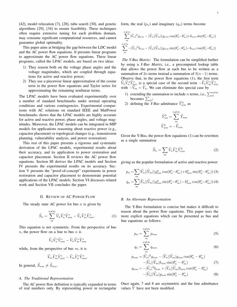
The experiments make two basic assumptions: (1) In theper unit system, voltages do not vary far from a magnitude of1.0 and angle of 0.0; (2) The magnitude of a line conductanceis much smaller than the magnitude of the susceptance, i.e.,|g| � |b|. We can then explore the bounds of the power flowequations (7) and (8), when the voltages are in the followingbounds: |Vn| = 1.0, |Vm| ∈ (1.2, 0.8), θ◦n−θ◦m ∈ (−π/6, π/6).These bounds are intentionally generous so that the power flowbehavior within and outside normal operating conditions maybe illustrated.
Figure 1 presents the contour of the active power (left)and reactive power (right) equations for a line 〈n,m〉 underthese assumptions when Ynm = 0.2 − i1. The contour linesindicate significant changes in power flow. Consider first theactive power plot (left). For a fixed voltage, varying the phase
4
Active Power Field
Voltage Difference
Ang
le D
iffer
ence
(ra
d)
−0.4
−0.3
−0.2
−0.1
0
0.1
0.2
0.3
0.4
0.8 0.9 1.0 1.1 1.2
−0.
4−
0.2
0.0
0.2
0.4
Reactive Power Field
Voltage DifferenceA
ngle
Diff
eren
ce (
rad)
−0.3
−0.25 −0.2 −0.15 −0.1
−0.05 0
0
0.05 0.1
0.8 0.9 1.0 1.1 1.2
−0.
4−
0.2
0.0
0.2
0.4
Fig. 1. Power Flow Contour of Active (left) and Reactive (right) Power withg = 0.2 and b = −1.
angle difference induces significant changes in active poweras many lines are crossed. In contrast, for a fixed phase angledifference, varying the voltage has limited impact on the activepower, since few lines are crossed. Hence, the plot indicatesthat phase angle differences are the primary factor of activepower flow while voltage differences have only a small effect.The situation is quite different for reactive power (right plot).For a fixed voltage, varying the phase angle difference inducessome significant changes in reactive power as around fourlines can be crossed. But, if the phase angle difference isfixed, varying voltage induces even more significant changesin reactive power since as many as seven lines may now becrossed. Hence, changes in voltages are the primary factor ofreactive power flows but the phase angle differences also havea significant influence.
B. The Hot-Start LPAC Model
The linear-programming approximation of the AC Powerflow equations in a hot-start context is based on three ideas:
1) It uses the voltage magnitude |V hn | from the AC base-
point solution at bus n;2) It approximates sin(x) by x;3) It uses a convex approximation of the cosine.1
Let cos(θ◦n−θ◦m) denote the convexification of cos(θ◦n−θ◦m) inthe range (−π/2, π/2), then the linear-programming approx-imation solves the line flow constraints
phnm = |V hn |2gnm − |V h
n ||V hm|gnmcos(θ◦n − θ◦m)
−|V hn ||V h
m|bnm(θ◦n − θ◦m) (10)
qhnm =−|V hn |2bnm + |V h
n ||V hm|bnmcos(θ◦n − θ◦m)
−|V hn ||V h
m|gnm(θ◦n − θ◦m) (11)
The details of the convexification are given in Appendix A.The hot-start model, presented in Model 1, is a linear programthat replaces the AC power equations by Equations 10 and 11and thus captures an approximation of reactive power in alinear formulation.
A complete linear program for this formulation is presentedin Model 1. The inputs to the model are: (1) A power networkPN = 〈N,L,G, s〉, where N is the set of buses, L is the setof lines, G is the set of voltage-controlled generators, s is
1The domain of the cosine should not exceed the range (−π/2, π/2) toensure convexity. This range is generous for AC power flows.
Model 1 The Hot-Start LPAC Model.Inputs:PN = 〈N,L,G, s〉 - the power network|V h| - voltage magnitudes from a base-point solutioncs - cosine approximation segment count
Variables:θ◦n ∈ (−∞,∞) - phase angle on bus n (radians)cosnm ∈ (0, 1) - Approximation of cos(θ◦n − θ◦m)
the slack bus; (2) the voltage magnitudes |V h| for the busesand (3) the number of segments cs for approximating thecosine function. The objective (M1.1) maximizes the cosineapproximation to make it as close as possible to the truecosine value. Constraints (M1.2) model the slack bus, whichhas a fixed phase angle. Constraints (M1.3) and (M1.4) modelKCL on the buses. Like in AC power flow models, the KCLconstraints are not enforced on the slack bus for both activeand reactive power and on voltage-controlled generators forreactive power. Constraints (M1.5) and (M1.6) capture theapproximate line flows from Equations (10) and (11). Finally,Constraints (M1.7) define a system of inequalities capturingthe piecewise-linear approximation of the cosine terms in thedomain (−π/3, π/3) using cs line segments for each line inthe power network.
To our knowledge, this hot-start model is the first linearformulation that captures the cosine contribution to reactivepower. However, fixing the voltage magnitudes, |V h|, in thepower flow equations may be too restrictive in many applica-tions. In the remaining sections, we remove this restriction.
C. The Warm-Start LPAC Model
This section derives the warm-start LPAC model, i.e., aLinear-Programming model of the AC power flow equationsfor the warm-start context. The warm-start context assumesthat some target voltages |V t| are available for all buses exceptvoltage-controlled generators whose voltage magnitudes |V g|are known. The network must operate close (e.g., ±0.1 Voltsp.u.) to these target voltages, since otherwise the hardwaremay be damaged or voltages may collapse.
The warm-start LPAC model is based on two key ideas:1) The active power approximation is the same as in the
hot-start model, with the target voltages replacing thevoltages in the base-point solution;
2) The reactive power approximation reasons about voltagemagnitudes, since changes in voltages are the primaryfactor of reactive power flows.
5
To derive the reactive power approximation in the warm-startLPAC model, let φ be the difference between the target voltageand the true value, i.e.,
|V | = |V t|+ φ.
Substituting in Equation 8, we obtain
qnm =−(|V tn|2 + 2|V t
n|φn + φ2n)bnm −
(|V tn||V t
m|+ |V tn|φm + |V t
m|φn + φnφm)
(gnm sin(θ◦n − θ◦m)− bnm cos(θ◦n − θ◦m)) (12)
We can divide this expression into two parts
qnm = qtnm + q∆nm (13)
where qtnm is Equation 8 with |V | = |V t| and q∆nm captures
the remaining terms, i.e.,
q∆nm =−(2|V t
n|φn + φ2n)bnm −
(|V tn|φm + |V t
m|φn + φnφm)
(gnm sin(θ◦n − θ◦m)− bnm cos(θ◦n − θ◦m)) (14)
Equation 13 is equivalent to Equation 8 and must be linearizedto obtain the LPAC model.
The qtnm part has target voltages and may thus be approx-imated like qhnm. The q∆
nm is more challenging as it containsnonlinear and non-convex terms such as φnφm cos(θ◦n − θ◦m).We approximate q∆
nm using the linear terms of the Taylor seriesof q∆
nm at φn = 0, φm = 0, θ◦n − θ◦m = 0 to obtain
q∆nm =−(2|V t
n|φn)bnm + (|V tn|φm + |V t
m|φn)bnm (15)
or, equivalently,
q∆nm =−|V t
n|bnm(φn − φm)− (|V tn| − |V t
m|)bnmφn (16)
A complete linear program for this formulation is presented inModel 2. The inputs to the model are similar to Model 1, withhot start voltages |V h| replaced by target voltages |V t|. Theobjective (M2.1) maximizes the cosine approximation to makeit as close as possible to the true cosine value. Constraints(M2.2) model the slack bus, which has a fixed voltage andphase angle. Constraints (M2.3) capture the voltage-controlledgenerators which, by definition, do not vary from their voltagetarget |V t|. Constraints (M2.4) and (M2.5) model KCL onthe buses, as well as the effects of voltage change presentedin Equation (16). Like in AC power flow models, the KCLconstraints are not enforced on the slack bus for both activeand reactive power and on voltage-controlled generators forreactive power. Constraints (M2.6) and (M2.7) capture theapproximate line flows from Equations (10) and (11). Con-straints (M2.8) model the effects of voltage change presentedin Equation (16). Finally, Constraints (M2.9) define a systemof inequalities capturing the piecewise-linear approximationof the cosine terms in the domain (−π/3, π/3) using cs linesegments for each line in the power network.
Model 2 The Warm-Start LPAC Model.Inputs:PN = 〈N,L,G, s〉 - the power network|V t| - target voltage magnitudescs - cosine approximation segment count
Variables:θ◦n ∈ (−∞,∞) - phase angle on bus n (radians)φn ∈ (−|V t|,∞) - voltage change on bus n (Volts p.u.)cosnm ∈ (0, 1) - Approximation of cos(θ◦n − θ◦m)
We now conclude by presenting the cold-start LPAC model.In a cold-start context, no target voltages are available andvoltage magnitudes are approximated by 1.0, except forvoltage-controlled generators whose voltages are given by |V g
n |(n ∈ G). The cold-start LPAC model is then derived from thewarm-start LPAC model by fixing |V t
i | = 1 for all i ∈ N .Equation (16) then reduces to
q∆nm =−bnm(φn − φm) (17)
Figure 3 presents the cold-start LPAC model, which is veryclose to the warm-start model. Note that Constraints (M3.3)use φi to fix the voltage magnitudes of generators.
E. Extensions to the LPAC Model
The LPAC models can be used to solve the AC power flowequations approximately in a variety of contexts. This sectionreviews how to generalize the LPAC models for applicationsin disaster management, reactive voltage support, transmissionplanning, and vulnerability analysis. The extensions are illus-trated on the warm-start model but can be similarly applied tothe cold-start model.
Generators: The LPAC model can easily be generalizedto include ranges for generators: Simply remove the generatorfrom G and place operating limits on the p and q variablesfor that bus. In this formulation, voltage-controlled generatorscan also be accommodated by fixing φn to zero at bus n.
Removing the Slack Bus: By necessity, AC solvers use aslack bus to ensure the flow balance in the network when thetotal power consumption is not known a priori (e.g., due to linelosses). As a consequence, the LPAC model depicted in Figure2 also uses a slack bus so that the AC and LPAC models canbe accurately compared in our experimental results. However,it is important to emphasize that the LPAC model does not
6
Model 3 The Cold-Start LPAC Model.Inputs:PN = 〈N,L,G, s〉 - the power networkcs - cosine approximation segment count
Variables:θ◦n ∈ (−∞,∞) - phase angle on bus n (radians)φn ∈ (−|V t|,∞) - voltage change on bus n (Volts p.u.)cosnm ∈ (0, 1) - Approximation of cos(θ◦n − θ◦m)
need a slack bus and the only reason to include a slack bus inthis model is to allow for meaningful comparisons between theLPAC and AC models. As discussed above, the LPAC modelcan easily include a range for each generator, thus removingthe need for a slack bus.
Load Shedding: For applications in power restoration(e.g., [45], [46], [51]), the LPAC model can also integrate loadshedding: Simply transform the loads into decision variableswith an upper bound and maximize the load served. The cosinemaximization should also be included in the objective but witha smaller weight. Section V-A reports experimental results onsuch a power restoration model.
Modeling Additional Constraints: In practice, feasibilityconstraints may exist on the acceptable voltage range, thereactive injection of a generator, or line flow capacities.Because Model 2 is a linear program, it can incorporate suchconstraints. For instance, constraint
|V | ≤ |V tn|+ φn ∀n ∈ N
ensures that voltages are above a certain limit |V |, constraint
n6=m∑m∈N
qtnm + q∆nm ≤ qn ∀n ∈ G
limits the maximum reactive injection bounds at bus n to qn.Finally, let |Snm| be the maximum apparent power on a linefrom bus n to bus m. Then, constraint
(ptnm)2 + (qtnm + q∆nm)2 ≤ |Snm|
2
ensures that line flows are feasible in the LPAC model. Thequadratic functions can be approximated by piecewise-linearconstrains (e.g., [50]).
IV. ACCURACY OF THE LPAC MODEL
This section evaluates the accuracy of the LPAC modelsby comparing them to an ideal nonlinear AC power flow.2
It includes a detailed analysis of the model accuracy (Sec-tion IV-A) and an investigation of alternative approximations(Section IV-B). The experiments were performed on ninetraditional power-system benchmarks which come from theIEEE test systems [57] and MATPOWER [58]. The AC powerflow equations were solved with a Newton-Raphson solverwhich was validated using MATPOWER. The LPAC modelsuse 20 line segments in the cosine approximation and allof the models solved in less than 1 second on a 2.5 GHzIntel processor. The results also include a modified version ofthe IEEEdd17 benchmark, called IEEEdd17m. The originalIEEEdd17 has the slack bus connected to the network bya transformer with |T | = 1.05. The nonlinear behavior oftransformers induces some loss of accuracy in the LPAC modeland, because this error occurs at the slack bus in IEEEdd17, itaffects all buses in the network. IEEEdd17m resolves this issueby setting |T | = 1.00 and the slack bus voltage to 1.05. Asthe results indicate, this equivalent formulation is significantlybetter for the LPAC model.
A. Accuracy of The LPAC Models
This section reports empirical evaluations of the LDC andLPAC models in cold-start and warm-start contexts. It reportsaggregate statistics for active power (Table I), bus phase angles(Table II), reactive power (Table III), and voltage magnitudes(Table IV). Data for the LDC model is necessarily omittedfrom Tables III and IV as reactive power and voltages are notcaptured by that model. In each table, two aggregate valuesare presented: Correlation (corr) and absolute error (∆). Theunits of the absolute error are presented in the headings. Bothaverage (µ) and worst-case (max) values are presented. Theworst case can often be misleading: For example a very largevalue may actually be a very small relative quantity. For thisreason, the tables show the relative error (δ) of the valueselected by the max operator using the arg-max operator. Therelative error is a percentage and is unit-less.
Table I indicates uniform improvements in active powerflows, especially in the largest benchmarks IEEE118,IEEEdd17, and MP300. Significant errors are not uncommonfor the linearized DC model on large benchmarks [47] and areprimarily caused by a lack of line losses. Due to its asymmet-rical power flow equations and the cosine approximation, theLPAC model captures line losses.
Table II presents the aggregate statistics on bus phase angles.These results show significant improvements in accuracy es-pecially on larger benchmarks. The correlations are somewhatlower than active power, but phase angles are quite challengingfrom a numerical accuracy standpoint.
Table III presents the aggregate statistics on line reactivepower flows. They indicate that reactive power flows are gen-erally accurate and highly precise in warm-start contexts. Tohighlight the model accuracy in cold-start contexts, the reactive
2For consistency, the LPAC models are extended to include line charging,bus shunts, and transformers, as discussed in Section II-C.
7
TABLE IACCURACY OF THE LPAC MODEL: ACTIVE POWER FLOWS.
Benchmark Active Power (MW)Corr µ(∆) max(∆) δ(arg-max(∆))
Fig. 2. Reactive Power Flow Correlation for the LPAC Model on IEEEdd17m(left) and MP300 (right) in a cold-start context.
flow correlation for the two worst benchmarks, IEEEdd17mand MP300, is presented in Figure 2.
Table IV presents the aggregate statistics on bus voltagemagnitudes. These results indicate that voltage magnitudes arevery accurate on small benchmarks, but the accuracy reduceswith the size of the network. The warm-start context brings asignificant increase in accuracy in larger benchmarks. To illus-trate the quality of these solutions in cold-start contexts, thevoltage magnitude correlation for the two worst benchmarks,i.e., IEEEdd17m and MP300, is presented in Figure 3. Theincrease in voltage errors is related to the distance from a loadpoint to the nearest generator. The linearized voltage modelincurs some small error on each line. As the voltage changes
Fig. 3. Voltage magnitude correlation for Model LPAC on IEEEdd17m (left)and MP300 (right) in a cold-start context.
over many lines, these small errors accumulate. By comparingthe percentage of voltage-controlled generator buses in eachbenchmark |G|/|N | (Table V) to accuracy in Table IV, theIEEE57 and IEEEdd17 benchmarks indicate that that a lowpercentage is a reasonable indicator of the voltage accuracy inthe cold-start context.
B. Alternative Linear Models
The formulation of the LPAC models explicitly removes twocore assumptions of the traditional LDC model:
1) Although cos(θ◦n − θ◦m) maybe very close to 1, thosesmall deviations are important.
8
TABLE IIIACCURACY OF THE LPAC MODEL: REACTIVE POWER FLOWS.
Benchmark Reactive Power (MVar)Corr µ(∆) max(∆) δ(arg-max(∆))
2) Although |g| � |b|, the conductance contributes signifi-cantly to the phase angles and voltage magnitudes.
This section investigates three variants of the cold-start LPACmodel that reintegrate some of the assumptions of the LDCmodel. The new models are: (1) the LPAC-C model where onlythe cosine approximation is used and g = 0; (2) the LPAC-Gmodel where only the g value is used and cos(x) = 1; (3)the LPAC-CG model where cos(x) = 1 and g = 0. TablesVI and VII present the cumulative absolute error between theproposed linear formulations and the true nonlinear solutions.Many metrics may be of interest but these results focus online voltage drop Vn − Vm and bus power Sn. These wereselected because they are robust to errors which accumulateas power flows through the network. The results highlight
TABLE VPERCENTAGE OF VOLTAGE-CONTROLLED BUSES IN THE BENCHMARKS.
two interesting points. First, all linear models tend to bringimprovements over a traditional LDC model. Second, althoughintegrating either the g value or the cosine term brings somesmall improvement independently, together they make signifi-cant improvements in accuracy. Additionally a comparison ofTable VI and Table VII reveals that the benefits of the newlinear models are more pronounced as the network increases.
V. CASE STUDIES
This section describes two case studies to evaluate thepotential of the LPAC models: Power restoration and capacitorplacement. The goal is not to present comprehensive solutionsfor these two complex problems, but to provide preliminaryevidence that the LPAC models may be useful in striking agood compromise between efficiency and accuracy for suchapplications. This section should be viewed as presenting a“proof-of-concept” that the LPAC models may be valuablefor certain classes of applications where the LDC model isnot accurate enough and existing approaches are too timeconsuming or suboptimal.
9
TABLE VIIACCURACY COMPARISON OF VARIOUS LINEAR MODELS (PART II).
Model Cumulative Absolute Error<(Vn−Vm) =(Vn−Vm) pn qn
After a significant disruption due to, say, a natural disaster,large sections of the power network need to be re-energized. Tounderstand the effects of restoration actions, power engineersmust simulate the network behaviour under various courses ofaction. However, the network is far from its normal operatingstate, which makes it extremely challenging to solve the ACpower flow equations. In fact, the task of finding an ACsolution without a reasonable starting point has been regardedas ”maddeningly difficult” [15]. The LPAC model studiedhere has the benefit of providing starting values for all thevariables in the AC power flow problem, unlike the traditionalLDC which only provides active power values. Furthermore,the LPAC model has the additional advantage of supportingbounds on reactive generation and voltage magnitudes andsuch constraints are critical for providing feasible solutionsto the AC power flow. This section illustrates these benefits.
Before presenting the power-restoration model, it is impor-tant to mention the key aspect of this application. When thepower system undergoes significant damages, load sheddingmust occur. The LDC and LPAC models must be embeddedin a restoration model that maximizes the served load givenoperational constraints such as the generation limits. Theseload values indicate the maximum amount of power that can bedispatched while ensuring system stability. Model 4 presentsa linear program based on the warm-start LPAC model which,given limits on active power generation pg and the desiredactive and reactive loads pl, ql at each bus, determines the
Model 4 A LP for Maximizing Desired Load.Inputs:
pgn - maximum active injection for bus npln - desired active load at bus nqln - desired reactive load at bus nInputs from Model 2 (The Warm-Start LPAC Model)
Variables:pgn ∈ (0, pgn) - active generation at bus nqgn ∈ (−∞,∞) - reactive generation at bus nln ∈ (0, 1) - percentage of load served at bus nVariables from Model 2 (The Warm-Start LPAC Model)
Maximize:∑n∈N
ln (M4.1)
Subject to:pn = −plnln + pgn ∀n ∈ N (M4.2)qn = −qlnln + qgn ∀n ∈ N (M4.3)qgn = 0 ∀n ∈ N \G (M4.4)
qn =
n 6=m∑m∈N
qtnm + q∆nm ∀n ∈ G (M4.5)
Constraints from Model 2 (The Warm-Start LPAC Model)
maximum amount of load that can be dispatched. The modelassumes that the loads can be shed continuously and that theactive and reactive parts of the load should maintain the samepower factor. The objective function (M4.1) maximizes thepercentage of served load. Constraints (M4.2) and (M4.3) setthe active and reactive injection at bus n appropriately basedon the decision variables for load shedding and generationdispatch. Constraint (M4.4) ensures that reactive generationonly occurs at generator buses and Constraint (M4.5) nowdefines qn for generator buses as well.
Since it reasons about reactive power and voltage magni-tudes, Model 4 can be further enhanced to impose bounds onthese values. As we will show, such bounds are often criticalto obtain high-quality solutions in power restoration contexts.If a reactive generation bound qg is supplied, this model canbe extended by adding the constraint,
qgn ≤ qgn ∀n ∈ N.
Voltage magnitude limits can also be incorporated. Givenupper and lower voltage limits |V | and |V |, the constraint
|V | ≤ 1.0 + φn ≤ |V | ∀n ∈ N.
may be used to enforce bounds on voltage magnitudes. Theexperimental results study the benefits of the LPAC model,suitably enhanced to capture these extensions, for powerrestoration. They compare a variety of linear models includingthe LDC model, the LPAC model, and enhancements of theLPAC model with additional constraints on reactive power andvoltage magnitudes.
Table VIII studies the applicability of various linear powermodels for network restoration on the IEEE30 benchmark.1000 line outage cases were randomly sampled from eachof the N −3, N −4, N −5, . . . , N −20 contingencies. Eachcontingency is solved with a linear power model (e.g., theLDC model or the LPAC model), whose solution is used asa starting point for the AC model. The performance metric
10
TABLE VIIIPOWER RESTORATION: ACHIEVING AC FEASIBILITY FROM DIFFERENT
is the number of cases where the AC solver converges, as agood linear model should yield a feasible generation dispatchwith a good starting point for the AC solver. To understand theimportance of various network constraints, four linear modelsare studied: the traditional LDC model; the LPAC model; theLPAC model with constraints on reactive generation (LPAC-R); and the LPAC with constraints on reactive generation andvoltage limits (LPAC-R-V). The number of solved models foreach of the contingency classes is presented in Table VIII.The results indicate that a traditional LDC model is overlyoptimistic and often produces power dispatches that do notlead to feasible AC power flows (the N−10 and N−13 areparticularly striking). However, each refinement of the LPACmodel solves more contingencies. The LPAC-R-V model isvery reliable and is able to produce feasible dispatches inall contingencies except 40 . This means that the LPAC-R-V model solves 99.76% of the 17,000 contingencies studied.Table IX depicts the load shed by the various models. For largecontingencies, the LPAC-R-V model not only provides goodstarting points for an AC solver but its load shedding is only
slightly larger than the (overly optimistic) LDC model. Theseresults provide compelling evidence of the benefits of theLPAC model for applications dealing with situations outsidethe normal operating conditions. In addition, Model 4 canreplace the LDC model in power restoration applications (e.g.,[45], [46]) that are using MIP models to minimize the size ofa blackout over time.
B. The Capacitor Placement Problem
The Capacitor Placement Problem (CPP) is a well-studiedapplication [28], [29], [30] and many variants of the problemexist. This section uses a simple version of the problem todemonstrate how the LPAC model can be used as a buildingblock inside a MIP solver for decision-support applications.
Informally speaking, the CPP consists of placing capacitorsthroughout a power network to improve voltage stability. Theversion studied here aims at placing as few capacitors aspossible throughout the network, while meeting a lower bound|V | on the voltages and satisfying a capacitor injection limit qc
and reactive generation limits qgn (n ∈ G). Model 5 presents aCPP model based on the cold-start LPAC model. For each busn, the additional decision variables are the amount of reactivesupport added by the capacitor qcn and a variable cn indicatingwhether a capacitor was used.
The objective function (M5.1) minimizes the number ofcapacitors. Constraints (M5.2) ensure the voltages do notdrop below the desired limit and do not exceed the preferredoperating condition of 1.05 Volts p.u. Constraints (M5.3) linkthe capacitor injection variables with the indicator variables, astandard technique in MIP models. Constraints (M5.4) ensureseach generator n ∈ G does not exceed its reactive generationlimit qgn. and constraints (M5.5) defines the reactive power forgenerators. Lastly, Constraints (M5.6) redefines the reactivepower equation to inject the capacitor contribution qc. Theremainder of the model is the same as Model 3 (the cold-startLPAC model).
The CPP model was tested on a modified version ofthe IEEE57 benchmark. All of the IEEE benchmarks havesufficient reactive support in their normal state. To make aninteresting capacitor placement problem, the transformer tapratios are set to 1.0 and existing synchronous condensers areremoved. This modified benchmark (IEEE57-C) has signif-icant voltage problems with several bus voltages droppingbelow 0.9. By design, a solution to Model 5 satisfies all of thedesired constraints. However, Model 5 is based on the LPACmodel and is only an approximation of the AC power flow. Tounderstand the true value of Model 5, we solve the resultingsolution network with an AC solver and measure how muchthe constraints are violated. Table X presents the results ofModel 5 on benchmark IEEE57-C with qc = 30 and variousthresholds |V |. The table presents the following quantities:The minimum desired voltage |V |; The worst violation ofthe voltage lower-bound min(|V |); The worst violation of thevoltage upper bound max(|V |); The worst violation of reactiveinjection upper bound max(qn); The number of capacitorsplaced
∑cn; and the runtime of the MIP to prove the optimal
placement solution. The table indicates that the CPP model is
11
Model 5 A MIP for the Capacitor Placement Problem.Inputs:
qgn - injection bound for generator nqc - capacitor injection bound|V | - minimum desired voltage magnitudeInputs from Model 3 (The Cold-Start LPAC Model)
Variables:qcn ∈ (0, qc) - capacitor reactive injectioncn ∈ {0, 1} - capacitor placement indicatorVariables from Model 3 (The Cold-Start LPAC Model)
extremely accurate and only has minor constraint violations onthe lower bounds of the voltage values. It is important to notethat, although the CPP model can take as long as five minutesto prove optimality3, it often finds the best solution valuewithin a few seconds. The voltage lower bound approachesthe value of 0.985, which is the lowest value of the voltage-controlled generators in the benchmark. These results remainconsistent for other voltage bounds.
Once again, the CPP model indicates the benefits of theLPAC approximation for decision-support applications thatneed to reason about reactive power and voltages.
VI. RELATED WORK
Many linearizations of the AC power flow equations havebeen developed [4], [6], [7], [16], [35], [39], [59]. Broadly,they can be grouped into iterative methods [6], [16], [59] andconvex models [4], [7], [35], [39].
Iterative Methods: Iterative methods, such as the fast-decoupled load flow [59], significantly reduce the computationtime of solving the AC equations and demonstrate sufficientaccuracy. Their disadvantage however is that they cannot beefficiently integrated into traditional decision-support tools.Indeed, MIP solvers require purely declarative models toobtain lower bounds that are critical in reducing the sizeof the search space. Note however that, modulo the linear
3It is of course only optimal up the quality of the LPAC approximation.
approximations, the LPAC model can be viewed as solving adecoupled load flow globally. The key differences are:
1) Because the model forms one large linear system, allof the steps of the decoupled load flow are effectivelysolved simultaneously;
2) Because the formulation is a linear program, the valuesof p and q can now be decision variables, and boundsmay be placed on the line capacities, voltage magni-tudes, and phase angles;
3) The model may be embedded in a MIP solver for makingdiscrete decisions about the power system.
The second and third points represent significant advantagesover the fast-decoupled load flow and other iterative methods.
Convex Models: Although many variants of the LDCmodel exist, few declarative models incorporate reactive flowsin cold-start contexts. To our knowledge, three cold-start ap-proaches have been proposed: (1) a polynomial approximationscheme [39], (2) a semi-definite programming relaxation [7],and (3) a voltage-difference model [35].
The polynomial approximation has the advantage of solvinga convex relaxation of the AC power equations but the numberof variables and constraints needed to model the relaxation”grows rapidly” [39] and only second-order terms were con-sidered. The accuracy of this approach for general powerflows remains an open question: Reference [39] focuses ona transmission planning application and does not quantify theaccuracy of the approximation relative to an AC power flow.
The semi-definite programming (SDP) relaxation [7] hasthe great advantage that it can solve the power flow equationsprecisely, without any approximation. In fact, reference [7]demonstrated that the formulation finds the globally optimalvalue to the AC optimal power flow problem on a number oftraditional benchmarks. However, recent work has shown thisdoes not hold on some practical examples [60]. Computation-ally, SDP solvers are also less mature than LP solvers and theirscalability remains an open question [61]. Solvers integratingdiscrete variables on top of SDP models [62] are very recentand do not have the scientific maturity of MIP solvers [48].
The voltage-difference model [35] has a resemblance to amodel combining the equation
phnm = |V hn |2gnm − |V h
n ||V hm|gnm − |V h
n ||V hm|bnm(θ◦n − θ◦m)
with Equation (17). However, it makes a fundamental assump-tion that all voltages are the same before computing the voltagedifferences. In practice, voltage-controlled generators violatethis assumption. On traditional power system benchmarks, weobserved that the voltage-difference formulation had similaraccuracy to the LDC model.
VII. CONCLUSION
This paper presented linear programs to approximate the ACpower flow equations. These linear programs, called the LPACmodels, capture both the voltage phase angles and magnitudes,which are coupled through equations for active and reactivepower. The models use a piecewise linear approximation ofthe cosine term in the power flow equations. The cold-start
12
−1.5 −1.0 −0.5 0.0 0.5 1.0 1.5
0.0
0.2
0.4
0.6
0.8
1.0
Quality of a Piece−wise Linear Cosine Approximation
Radians
cos(x)ConstraintFeasible Region
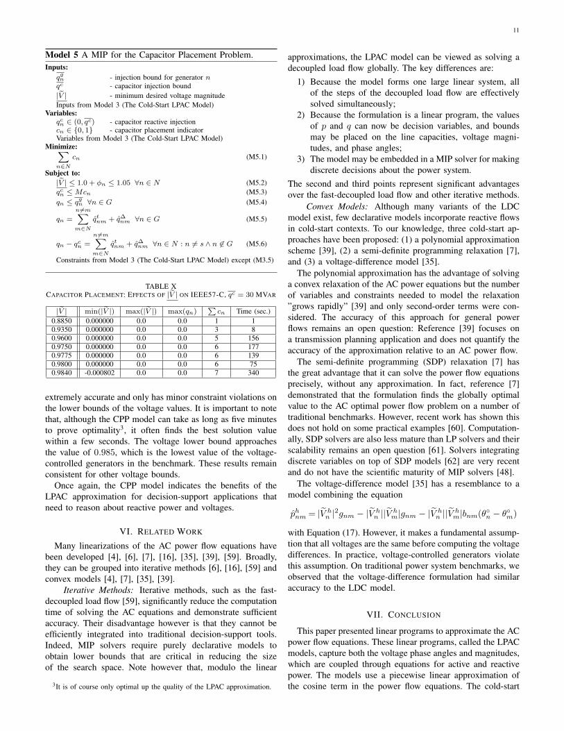
Fig. 4. A Piecewise-Linear Approximation of Cosine using 7 Inequalities.
and warm-start models use a Taylor series for approximatingthe remaining nonlinear terms.
The LPAC models have been evaluated experimentally overa number of standard benchmarks under normal operating con-ditions and under contingencies of various sizes. Experimentalcomparisons with AC solutions on a variety of standard IEEEand MatPower benchmarks shows that the LPAC models arehighly accurate for active and reactive power, phase angles,and voltage magnitudes. The paper also presented two casestudies in power restoration and capacitor placement to provideevidence that the cold-start and wam-start LPAC models can beefficiently used as a building block for optimization problemsinvolving constraints on reactive power flow and voltagemagnitudes. As a result, the LPAC models have the potentialto broaden the success of the traditional LDC model intonew application areas and to bring increased accuracy andreliability to current LDC applications.
There are many opportunities for further study, including theapplication of the LPAC models to a number of applicationareas. From an analysis standpoint, it would be interestingto compare the LPAC models with an AC solver using a“distributed slack bus”. Such an AC solver models the realpower systems more accurately and provides a better basis forcomparison, since the LPAC models are easily extended toflexible load and generation at all buses.
APPENDIX AA LINEAR PROGRAMMING APPROXIMATION OF COSINE
The convex approximation of the cosine function is imple-mented through a piecewise linear function that produces alinear program in the following way. The modeler selectsa desired domain (l, h)4 and a number segments s. Then stangent inequalities are placed on the cosine function withinthe provided domain to approximate the convex region. Figure4 illustrates the approximation approach using seven linearinequalities. The dark black line shows the cosine function,the dashed lines are the linear inequality constraints, andthe shaded area is the feasible region of the linear systemformed by those constraints. The inequalities are obtained fromtangents lines at various points on the function. Specifically,
4The domain should not exceed the range (−π/2, π/2) to ensure convexity.In practice, θ◦n − θ◦m is typically very small and a narrower domain ispreferable.
PWL<COS>(xcos, x, l, h, s)
1 post(xcos ≥ cos(h)−cos(l)h−l (x− l) + cos(l))
2 inc← (h− l)/(s+ 1)3 a← l + inc4 for i ∈ 1..s5 do fa ← cos(a)6 sa ← − sin(a)7 post(xcos ≤ sax− saa+ fa)8 a← a+ inc
for an x-coordinate a, the tangent line is y = − sin(a)(x−a)+cos(a) and, within the domain of (−π/2, π/2), the inequality
y ≤ − sin(a)(x− a) + cos(a) ∀a
holds. Figure 5 gives an algorithm to generate s inequalitiesevenly spaced within (l, h). In the algorithm, x is a decisionvariable used as an argument of the cosine function and xcos isa decision variable capturing the approximate value of cos(x).
REFERENCES
[1] J. A. Momoh, Electric Power System Applications of Optimization(Power Engineering (Willis)). CRC Press, 2001.
[2] A. Ott, “Unit commitment in the pjm day-ahead and real-time markets,”http://www.ferc.gov/eventcalendar/Files/20100601131610-Ott,2010, ac-cessed: 22/04/2012.
[3] J. Miller, “Power system optimization smart grid, de-mand dispatch, and microgrids,” Published online athttp://www.netl.doe.gov/smartgrid/referenceshelf/presentations/SESept.2011, accessed: 22/04/2012.
[4] Z. Wang, D. Peng, Q. Feng, H. Liu, and D. C. Yu, “A non-incrementalmodel for optimal control of reactive power flow,” Electric PowerSystems Research, vol. 39, no. 2, pp. 153 – 159, 1996.
[5] P. K. C. Aniruddha Bhattacharya, “Solution of optimal reactive powerflow using biogeography-based optimization,” International Journal ofElectronics and Electrical Engineering, vol. 4, no. 8, pp. 568 – 576,2010.
[6] D. Thukaram, K. Parthasarathy, and D. Prior, “Improved algorithm foroptimum reactive power allocation,” International Journal of ElectricalPower and Energy Systems, vol. 6, no. 2, pp. 72 – 74, 1984.
[7] J. Lavaei and S. Low, “Zero duality gap in optimal power flow problem,”IEEE Transactions on Power Systems, vol. 27, no. 1, pp. 92 –107, feb.2012.
[8] S. Granville, “Optimal reactive dispatch through interior point methods,”IEEE Transactions on Power Systems, vol. 9, no. 1, pp. 136 –146, feb1994.
[9] P. Sreejaya and S. Iyer, “Optimal reactive power flow control for voltageprofile improvement in ac-dc power systems,” in Joint InternationalConference on Power Electronics, Drives and Energy Systems (PEDES)2010 India, dec. 2010, pp. 1 –6.
[10] N. Deeb and S. Shahidehpour, “Linear reactive power optimizationin a large power network using the decomposition approach,” IEEETransactions on Power Systems, vol. 5, no. 2, pp. 428 –438, may 1990.
[11] V. Ajjarapu, P. L. Lau, and S. Battula, “An optimal reactive powerplanning strategy against voltage collapse,” IEEE Transactions on PowerSystems, vol. 9, no. 2, pp. 906 –917, may 1994.
[12] D. Kirschen and H. Van Meeteren, “Mw/voltage control in a linearprogramming based optimal power flow,” IEEE Transactions on PowerSystems, vol. 3, no. 2, pp. 481 –489, may 1988.
[13] J. Momoh, R. Adapa, and M. El-Hawary, “A review of selected optimalpower flow literature to 1993. i. nonlinear and quadratic programmingapproaches,” IEEE Transactions on Power Systems, vol. 14, no. 1, pp.96 –104, feb 1999.
[14] J. Momoh, M. El-Hawary, and R. Adapa, “A review of selected optimalpower flow literature to 1993. ii. newton, linear programming andinterior point methods,” IEEE Transactions on Power Systems, vol. 14,no. 1, pp. 105 –111, feb 1999.
[15] T. Overbye, X. Cheng, and Y. Sun, “A comparison of the ac and dcpower flow models for lmp calculations,” in Proceedings of the 37thAnnual Hawaii International Conference on System Sciences, 2004.
13
[16] A. R. S.G. Seifossadat, M. Saniei, “Reactive power pricing in compet-itive electric markets using a sequential linear programming with con-sidered investment cost of capacitor banks,” The International Journalof Innovations in Energy Systems and Power, vol. 1, April 2009.
[17] J. R. A. Munoz, “Analysis and application of optimization techniquesto power system security and electricity markets,” Ph.D. dissertation,University of Waterloo, 2008.
[18] E. Fisher, R. O’Neill, and M. Ferris, “Optimal transmission switching,”IEEE Transactions on Power Systems, vol. 23, no. 3, pp. 1346–1355,2008.
[19] K. Hedman, R. O’Neill, E. Fisher, and S. Oren, “Optimal transmissionswitching with contingency analysis,” IEEE Transactions on PowerSystems, vol. 24, no. 3, pp. 1577–1586, aug. 2009.
[20] A. Khodaei and M. Shahidehpour, “Transmission switching in security-constrained unit commitment,” IEEE Transactions on Power Systems,vol. 25, no. 4, pp. 1937 –1945, nov. 2010.
[21] B. Wollenberg and W. Stadlin, “A real time optimizer for securitydispatch,” IEEE Transactions on Power Apparatus and Systems, vol.PAS-93, no. 5, pp. 1640 –1649, sept. 1974.
[22] B. Stott, J. Marinho, and O. Alsac, “Review of linear programmingapplied to power system rescheduling,” in Power Industry ComputerApplications Conference, 1979 (PICA-79), may 1979, pp. 142 – 154.
[23] F. Lee, J. Huang, and R. Adapa, “Multi-area unit commitment viasequential method and a dc power flow network model,” IEEE Trans-actions on Power Systems, vol. 9, no. 1, pp. 279 –287, feb 1994.
[24] M. Shahidehpour, H. Yamin, and Z. Li, Market Operations in ElectricPower Systems: Forecasting, Scheduling, and Risk Management. Wiley-IEEE Press, 2002.
[25] H. Pinto, F. Magnago, S. Brignone, O. Alsac, and B. Stott, “Securityconstrained unit commitment: Network modeling and solution issues,”in Power Systems Conference and Exposition, 2006. PSCE ’06. 2006IEEE PES, 29 2006-nov. 1 2006, pp. 1759 –1766.
[26] C. A. N. A Borghetti, M Paolone, “A Mixed Integer Linear Program-ming Approach to the Optimal Configuration of Electrical DistributionNetworks with Embedded Generators,” Proceedings of the 17th PowerSystems Computation Conference (PSCC’11), Stockholm, Sweden, 2011.
[27] E. Romero-Ramos, J. Riquelme-Santos, and J. Reyes, “A simpler andexact mathematical model for the computation of the minimal powerlosses tree,” Electric Power Systems Research, vol. 80, no. 5, pp. 562 –571, 2010.
[28] P. C. Roberto S. Aguiar, “Capacitor placement in radial distribution net-works through a linear deterministic optimization model,” Proceedingsof the 15th Power Systems Computation Conference (PSCC’05), Lige,Belgium, 2005.
[29] M. Delfanti, G. Granelli, P. Marannino, and M. Montagna, “Optimalcapacitor placement using deterministic and genetic algorithms,” IEEETransactions on Power Systems, vol. 15, no. 3, pp. 1041 –1046, aug2000.
[30] Y.-C. Huang, H.-T. Yang, and C.-L. Huang, “Solving the capacitorplacement problem in a radial distribution system using tabu searchapproach,” IEEE Transactions on Power Systems, vol. 11, no. 4, pp.1868 –1873, nov 1996.
[31] D. Bienstock and S. Mattia, “Using mixed-integer programming to solvepower grid blackout problems,” Discrete Optimization, vol. 4, no. 1, pp.115– 141, 2007.
[32] M. K. Mangoli, K. Y. Lee, and Y. M. Park, “Optimal long-term reac-tive power planning using decomposition techniques,” Electric PowerSystems Research, vol. 26, no. 1, pp. 41 – 52, 1993.
[33] A. Hughes, G. Jee, P. Hsiang, R. Shoults, and M. Chen, “Optimalreactive power planning,” IEEE Transactions on Power Apparatus andSystems, vol. PAS-100, no. 5, pp. 2189 –2196, may 1981.
[34] K. Lee and F. Yang, “Optimal reactive power planning using evolu-tionary algorithms: a comparative study for evolutionary programming,evolutionary strategy, genetic algorithm, and linear programming,” IEEETransactions on Power Systems, vol. 13, no. 1, pp. 101 –108, feb 1998.
[35] A. M. C. A. Koster and S. Lemkens, “Designing ac power grids usinginteger linear programming,” in INOC, ser. Lecture Notes in ComputerScience, J. Pahl, T. Reiners, and S. Voß, Eds., vol. 6701. Springer,2011, pp. 478–483.
[36] R. Jabr, “Optimal placement of capacitors in a radial network usingconic and mixed integer linear programming,” Electric Power SystemsResearch, vol. 78, no. 6, pp. 941 – 948, 2008.
[37] X. Wang and J. McDonald, Modern Power System Planning. Mcgraw-Hill (Tx), 1994.
[38] J. dos Santos, A., P. Franca, and A. Said, “An optimization modelfor long-range transmission expansion planning,” IEEE Transactions onPower Systems, vol. 4, no. 1, pp. 94 –101, feb 1989.
[39] J. Taylor and F. Hover, “Linear relaxations for transmission systemplanning,” IEEE Transactions on Power Systems, vol. 26, no. 4, pp.2533 –2538, nov. 2011.
[40] J. Salmeron, K. Wood, and R. Baldick, “Analysis of electric grid securityunder terrorist threat,” IEEE Transactions on Power Systems, vol. 19,no. 2, pp. 905– 912, 2004.
[41] ——, “Worst-case interdiction analysis of large-scale electric powergrids,” IEEE Transactions on Power Systems, vol. 24, no. 1, pp. 96–104, 2009.
[42] N. Peterson, W. Tinney, and D. Bree, “Iterative linear ac power flowsolution for fast approximate outage studies,” IEEE Transactions onPower Apparatus and Systems, vol. PAS-91, no. 5, pp. 2048 –2056,sept. 1972.
[43] P. Ruiz and P. Sauer, “Post-contingency voltage and reactive powerestimation and large error detection,” in Power Symposium, 2007. NAPS’07. 39th North American, 30 2007-oct. 2 2007, pp. 266 –272.
[44] D. Bienstock and A. Verma, “The n-k problem in power grids: Newmodels, formulations, and numerical experiments,” SIAM Journal onOptimization, vol. 20, no. 5, pp. 2352–2380, 2010.
[45] C. Coffrin, P. Van Hentenryck, and R. Bent, “Strategic stockpiling ofpower system supplies for disaster recovery.” Proceedings of the 2011IEEE Power & Energy Society General Meetings (PES), 2011.
[46] P. Van Hentenryck, C. Coffrin, and R. Bent, “Vehicle routing for thelast mile of power system restoration,” Proceedings of the 17th PowerSystems Computation Conference (PSCC’11), Stockholm, Sweden, 2011.
[47] B. Stott, J. Jardim, and O. Alsac, “Dc power flow revisited,” IEEETransactions on Power Systems, vol. 24, no. 3, pp. 1290–1300, 2009.
[48] R. Bixby, M. Fenelon, Z. Gu, E. Rothberg, and R. Wunderling, Sys-tem Modelling and Optimization: Methods, Theory, and Applications.Kluwer Academic Publishers, 2000, ch. MIP: Theory and practice –closing the gap, pp. 19–49.
[49] K. Purchala, L. Meeus, D. Van Dommelen, and R. Belmans, “Usefulnessof DC power flow for active power flow analysis,” Power EngineeringSociety General Meeting, pp. 454–459, 2005.
[50] C. Coffrin, P. Van Hentenryck, and R. Bent, “Approximating Line Lossesand Apparent Power in AC Power Flow Linearizations,” Proceedings ofthe 2012 IEEE Power & Energy Society General Meetings (PES), 2012.
[51] ——, “Smart Load and Generation Scheduling for Power SystemRestoration,” Proceedings of the 2012 IEEE Power & Energy SocietyGeneral Meetings (PES), 2012.
[52] U. G. Knight, Power systems engineering and mathematics, by U. G.Knight. Pergamon Press Oxford, New York,, 1972.
[53] A. J. Wood and B. F. Wollenberg, Power Generation, Operation, andControl. Wiley-Interscience, 1996.
[54] L. Powell, Power System Load Flow Analysis (Professional Engineer-ing). McGraw-Hill Professional, 2004.
[55] A. Gomez-Exposito, A. J. Conejo, and C. Canizares, Electric EnergySystems: Analysis and Operation (Electric Power Engineering Series).CRC Press, 2008.
[56] J. Grainger and W. S. Jr., Power System Analysis. McGraw-HillScience/Engineering/Math, 1994.
[57] U. of Washington Electrical Engineering, “Power systems testcase archive,” http://www.ee.washington.edu/research/pstca/, accessed:30/04/2012.
[58] R. Zimmerman, C. Murillo-S andnchez, and R. Thomas, “Matpower:Steady-state operations, planning, and analysis tools for power systemsresearch and education,” IEEE Transactions on Power Systems, vol. 26,no. 1, pp. 12 –19, feb. 2011.
[59] B. Stott and O. Alsac, “Fast decoupled load flow,” IEEE Transactionson Power Apparatus and Systems, vol. 93, no. 3, pp. 859–869, 1974.
[60] B. Lesieutre, D. Molzahn, A. Borden, and C. DeMarco, “Examiningthe limits of the application of semidefinite programming to powerflow problems,” in 49th Annual Allerton Conference on Communication,Control, and Computing (Allerton), 2011, sept. 2011, pp. 1492 –1499.
[61] H. Mittelmann, “Benchmarks for optimization software,”http://plato.asu.edu/bench.html, April 2012, accessed: 22/04/2012.
[62] J. Lofberg, “Yalmip : a toolbox for modeling and optimization inmatlab,” in 2004 IEEE International Symposium on Computer AidedControl Systems Design, sept. 2004, pp. 284 –289.