A LOCAL FOURIER ANALYSIS FRAMEWORK FORFINITE-ELEMENT DISCRETIZATIONS OF SYSTEMS OF PDES∗

SCOTT P. MACLACHLAN†AND CORNELIS W. OOSTERLEE ‡

Abstract. Since their popularization in the late 1970s and early 1980s, multigrid methods havebeen a central tool in the numerical solution of the linear and nonlinear systems that arise from thediscretization of many PDEs. In this paper, we present a local Fourier analysis (LFA, or local modeanalysis) framework for analyzing the complementarity between relaxation and coarse-grid correctionwithin multigrid solvers for systems of PDEs. Important features of this analysis framework includethe treatment of arbitrary finite-element approximation subspaces and overlapping multiplicative-Schwarz type smoothers. The resulting tools are demonstrated for the Stokes, curl-curl, and grad-divequations.

1. Introduction. First envisioned as a technique for solving Poisson-type prob-lems with optimal complexity, multigrid and other multilevel algorithms have becomethe methods of choice for solving the matrix equations that arise in a wide variety ofapplications. In this paper, we are concerned with the design and analysis of multi-grid algorithms for the solution of discretized systems of partial differential equations.While general principles exist that can aid in developing multigrid techniques for anapplication area, the optimal choices for its components are often difficult to deter-mine beforehand. Many approaches to multigrid theory have been investigated in thelast 30 years (see, for example, [8, 17, 22, 33]); among these, the technique of localFourier analysis (LFA, or local mode analysis), first introduced in [9], has remainedvery successful, providing accurate predictions of performance for a variety of prob-lems, including for systems of PDEs.

The primary advantage of LFA is that it allows quantitative prediction of multi-grid convergence factors under reasonable assumptions. The word, local, in LFAindicates a focus on the character of an operator in the interior of its domain, whereit is assumed to be represented by a constant discretization stencil. The Fouriersymbols of such operators can easily be computed. A further insight in [41] wasthat all of the components in a multigrid method can be analyzed in this fashion,leading to a block-diagonal representation in a Fourier basis. LFA helped, for ex-ample, in the understanding of SOR as a smoother for moderately anisotropic andhigh-dimensional problems [50] and the solution of the biharmonic equation with ef-ficiency similar to that of Poisson [46]. Recent advances in LFA include LFA forhigh-dimensional problems [52], for multigrid as a preconditioner [47], for triangu-lar and hexagonal meshes [19, 51], optimal control problems [5], and discontinuousGalerkin discretizations [23]. The LFA monograph and related software of Wienandsand Joppich [46] focus on LFA for collocated discretizations, providing an excellenttool for experimenting with Fourier analysis.

In this paper, we present a framework for performing the local Fourier analysisfor state-of-the-art finite-element discretizations of systems of PDEs. In particular,

∗In preparation. This research was supported by the European Community’s Sixth FrameworkProgramme, through a Marie Curie International Incoming Fellowship, MIF1-CT-2006-021927. Thework of SM was partially supported by the National Science Foundation, under grant DMS-0811022.

†Delft University of Technology, Faculty of Electrical Engineering, Mathematics and ComputerScience, Mekelweg 4, 2628 CD Delft, The Netherlands and CWI, National Research Institute forMathematics and Computer Science, Amsterdam, The Netherlands. c.w.oosterlee@cwi.nl

‡Department of Mathematics, Tufts University, 503 Boston Avenue, Medford, MA 02155, USA.Formerly at TU-Delft and CWI. scott.maclachlan@tufts.edu

1

we show that the LFA ansatz is still valid when using overlapping multiplicativesmoothers, such as were proposed in [2], for the grad-div and curl-curl equations, andin [28,43] for the Stokes equations. Analysis of the additive versions of these smootherswas conducted in [4, 39]; however this form of analysis does not extend to cover themultiplicative case. LFA for overlapping multiplicative smoothers has been, to ourknowledge, performed in only two cases, for the staggered finite-difference discretiza-tion of the Stokes and Navier-Stokes equations [40], and for a mixed finite-elementdiscretization of Poisson’s equation [34]. We also apply this analysis to the well-knownmultigrid solvers for the grad-div, curl-curl, and Stokes equations, providing quanti-tative predictions of the performance of multigrid methods based on these smoothers,in contrast to the non-predictive proofs of convergence offered in [2,32]. In the case ofthe Stokes equations, in particular, quantitative estimates have been notably missingfrom the literature [31].

The remainder of this paper is organized as follows. First, in Section 2, we pro-vide some background on the motivating PDE systems for this work. LFA smoothinganalysis is discussed in Section 3, with a focus on the treatment of overlapping multi-plicative smoothers. A detailed example is presented in Section 4. Section 5 presentstwo-grid LFA, focusing on the issue of multigrid grid transfers for staggered discretiza-tions. Finally, Section 6 presents the application of these techniques to appropriatediscretizations of the Stokes, grad-div, and curl-curl equations. There, we focus onthe impact of the choice of transfer operators and on the choice of smoother andunder-relaxation parameters on the two-grid LFA convergence.

2. Multigrid and Finite Elements for PDE Systems. The discretizationof systems of PDEs must be done with care, to avoid the introduction of unstablemodes in the resulting discrete system. In finite elements, this typically results inchoosing different finite-element subspaces for different components of the system, tosatisfy known inf-sup conditions, leading to the use of Raviart-Thomas, Nedelec, orTaylor-Hood elements, for example. For a thorough treatment of these issues in thefinite-element context, see [6, 12].

We shall refer to the finite-element discretizations that we treat here collectivelyas ”staggered discretizations”, indicating that the nodes associated with the discretedegrees of freedom are not aligned on the same grid for each component of the PDEsystem. The techniques developed here are applicable to arbitrary staggered dis-cretizations of systems of PDEs, including the “trivial” case of a collocated discretiza-tion.

2.1. Multigrid for Systems of Equations. Many standard discretizations ofsystems of PDEs (including those described below) do not guarantee that the result-ing matrices are diagonally dominant (or even that they are definite) either becauseof the properties of the continuum operators themselves, or because of necessary con-straints on the discretizations. In these cases, expensive relaxation techniques maybe used to reestablish effective multigrid convergence. Unfortunately, these relax-ation techniques are no longer algebraic black boxes, like the Jacobi and Gauss-Seideliterations. Instead, the details of these techniques are determined by those of theunderlying PDEs.

A first indication for the appropriate choice of relaxation method for a system ofequations can be derived from the systems’ determinant. Interestingly, the determi-nant of the discrete operator may also give us valuable information about the stabilityof the discretizations used for a system. The direct relation between effectiveness ofsmoothing and the determinant of the discrete system is by means of the h-ellipticity

2

concept [10,42]. For unstable discretizations, which give rise to unphysical oscillationsin the numerical solutions, there is no chance that we can set up efficient local, i.e.,pointwise, smoothing methods.

An obvious choice in the case of strong off-diagonal operators in the differentialsystem (also indicated by the determinant) is collective smoothing: All unknowns inthe system at a certain grid point or grid cell are updated simultaneously. While theuse of these smoothers leads to efficient multigrid approaches for systems of PDEs,collective relaxation is not the only possible approach. The main alternative is theuse of distributive smoothers [10, 20, 24], which take their name from a distributionoperation; the discrete (or continuum) equations are transformed by right matrixmultiplication into a block triangular matrix that is amenable to pointwise relaxation.Simple pointwise relaxation is performed on this block triangular system and, then,the resulting update is distributed (based on the transformation matrix) back to theoriginal matrix problem.

While distributed smoothers are often found to be more efficient than overlap-ping smoothers [20], their applicability is limited by the need to find an effectivedistribution matrix; this is often difficult to do for problems with unstructured gridsor variable coefficients. Thus, distributed relaxation may be difficult to implementin a general and purely algebraic fashion, as would be necessary for use within analgebraic multigrid iteration. Furthermore, the proper treatment of boundary con-ditions in distributive relaxation may not be trivial, as typically the operator of thepreconditioned system is of higher order than the original operator, thus requiringadditional (possible nonphysical) boundary conditions within smoothing. Substantialeffort has however been put into successfully extending the distributed smoother ofHiptmair [24] to algebraic multigrid algorithms for the curl-curl equation [3, 27, 38].In this paper, we focus exclusively on collective relaxation approaches.

2.2. Discretizing Systems of PDEs. As a first pair of examples, we considerthe gradient-divergence (grad-div) and curl-curl equations,

−∇(a∇ · U) + U = F , inΩ, (2.1)

and

∇× (a∇× U) + U = F , inΩ, (2.2)

with parameter a > 0, where Ω is an open domain in Rd. These operators appearfrequently in the formulation of mathematical models in physics and engineering,particularly for problems related to electro-magnetics or fluid and solid mechanics(see, for example, [2, 20,25] for more details).

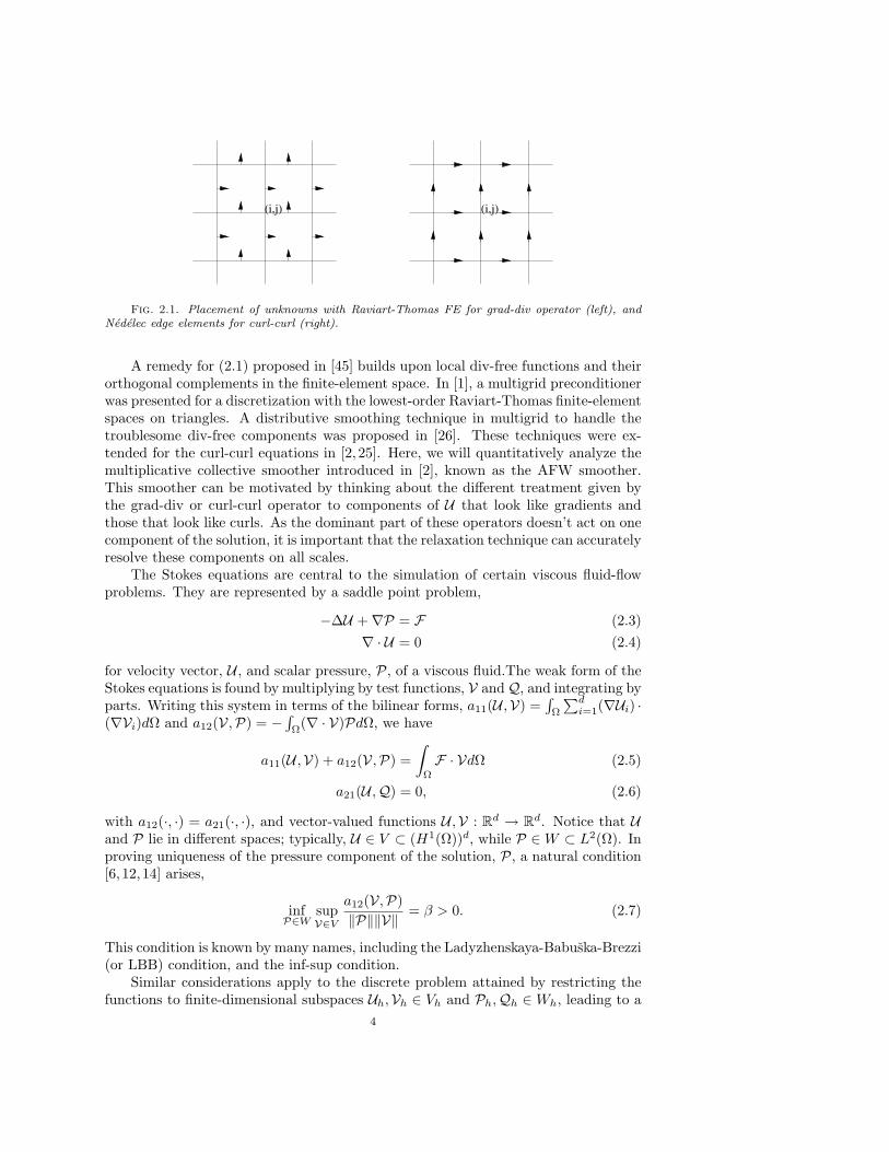
In the finite-element framework, face elements, such as the Raviart-Thomas el-ements, have been proposed for accurate discretization of (2.1) [37], while edge ele-ments, such as the Nedelec elements [35] are commonly used for (2.2), see Figure 2.2.The difficulty in achieving efficient multigrid treatment of the resulting discrete linearsystems comes from the fact that the eigenspace associated with the minimal eigen-value of the discrete operator contains many eigenvectors (for large enough parametera). For Equation (2.1), this arises because any divergence-free vector is an eigenvectorcorresponding to this minimal eigenvalue, while a similar difficulty occurs with curl-free vectors in (2.2). In both cases, these components can be arbitrarily oscillatoryand can neither be reduced by standard (pointwise) smoothing procedures, nor bewell represented on coarse grids [2].

3

(i,j) (i,j)

Fig. 2.1. Placement of unknowns with Raviart-Thomas FE for grad-div operator (left), andNedelec edge elements for curl-curl (right).

A remedy for (2.1) proposed in [45] builds upon local div-free functions and theirorthogonal complements in the finite-element space. In [1], a multigrid preconditionerwas presented for a discretization with the lowest-order Raviart-Thomas finite-elementspaces on triangles. A distributive smoothing technique in multigrid to handle thetroublesome div-free components was proposed in [26]. These techniques were ex-tended for the curl-curl equations in [2, 25]. Here, we will quantitatively analyze themultiplicative collective smoother introduced in [2], known as the AFW smoother.This smoother can be motivated by thinking about the different treatment given bythe grad-div or curl-curl operator to components of U that look like gradients andthose that look like curls. As the dominant part of these operators doesn’t act on onecomponent of the solution, it is important that the relaxation technique can accuratelyresolve these components on all scales.

The Stokes equations are central to the simulation of certain viscous fluid-flowproblems. They are represented by a saddle point problem,

−∆U +∇P = F (2.3)∇ · U = 0 (2.4)

for velocity vector, U , and scalar pressure, P, of a viscous fluid.The weak form of theStokes equations is found by multiplying by test functions, V andQ, and integrating byparts. Writing this system in terms of the bilinear forms, a11(U ,V) =

∫Ω

∑di=1(∇Ui) ·

(∇Vi)dΩ and a12(V,P) = −∫Ω(∇ · V)PdΩ, we have

a11(U ,V) + a12(V,P) =∫

Ω

F · VdΩ (2.5)

a21(U ,Q) = 0, (2.6)

with a12(·, ·) = a21(·, ·), and vector-valued functions U ,V : Rd → Rd. Notice that Uand P lie in different spaces; typically, U ∈ V ⊂ (H1(Ω))d, while P ∈W ⊂ L2(Ω). Inproving uniqueness of the pressure component of the solution, P, a natural condition[6, 12,14] arises,

infP∈W

supV∈V

a12(V,P)‖P‖‖V‖

= β > 0. (2.7)

This condition is known by many names, including the Ladyzhenskaya-Babuska-Brezzi(or LBB) condition, and the inf-sup condition.

Similar considerations apply to the discrete problem attained by restricting thefunctions to finite-dimensional subspaces Uh,Vh ∈ Vh and Ph,Qh ∈ Wh, leading to a

4

discrete version of the inf-sup condition. A natural discretization, representing bothUh and Ph with bilinear basis functions does not satisfy the necessary inf-sup condition[18] and, so, we are forced to consider higher-order basis functions for Equations(2.3) and (2.4), such as the Taylor-Hood elements [6, 21] where Uh is represented bybiquadratic basis functions and Ph is represented by bilinears.

The development of efficient smoothers for the Stokes equations was originallyperformed in the staggered finite-differences setting. There, the concepts of collectiveand distributive relaxation were developed, by Vanka [43] and Brandt and Dinar [10,11], respectively. These smoothers were later accompanied by quantitative analysis,based on LFA. For FE discretizations, work on efficient smoothers for the Stokes andNavier-Stokes equations includes that by Braess and Sarazin [7], which is based on anapproximate factorization of (2.3) and (2.4), as well as that by John and others [28,29,31, 49], which focuses on a variety of smoothers including those of collective (Vanka)type.

It was the FE setting especially that drove the rapid development of the algebraicmultigrid method in the nineties (of the last century), with the recognition of itsimpressive efficiency, often for completely unstructured meshes. Quantitative theoryfor methods on this type of meshes is not available, unfortunately. To bridge the gapbetween the fully understood case of finite differences on structured grids and thecase of finite elements on completely unstructured grids, we develop here quantitativeanalysis for FE discretizations on structured quadrilateral meshes in 2D, still leadingto stencil-based discretizations.

3. Analysis of relaxation with LFA. A quantitative, predictive theoreticalframework, such as LFA, allows significant algorithmic development independent ofan implementation. Here and in Section 5, we review the ideas behind two-grid localFourier analysis; first, we focus on the analysis of the smoothing step in Fourierspace. We consider the solution of a linear system of equations, Ahuh = fh, where thesubscript, h, serves to remind us that the origins of matrix Ah are in the discretizationof a PDE on a uniform quadrilateral grid with meshsize h (or, possibly, with meshsizesh = (hx, hy, . . .)T that are not uniform across dimensions).

Given an approximation, vh, to the solution of Ahuh = fh, the residual equationrelates the error, eh = uh−vh, in that approximation to the residual, rh = fh−Ahvh,as Aheh = rh. Thus, for a given approximation, vh, we can express the true solutionas uh = vh+A−1

h rh. Choosing Mh to be an approximation to Ah that is easily invertedleads to an update iteration that can be analyzed in terms of its error-propagationoperator

eh ←(I −M−1

h Ah

)eh.

A complete analysis of the convergence properties of the error propagation opera-tor arises in terms of its eigenvectors, φ(j), and eigenvalues, λj. Any initial error,e(0)

h , can then be expanded into the basis given by the eigenvectors of I −M−1h Ah,

and the error after k iterations of relaxation is given by e(k)h =

∑j σjλ

kj φ(j), where

the coefficients, σj, are defined so that the expansion is valid for the initial error,e(0)

h . The effectiveness of the relaxation on the component of the error in the direc-tion of a given eigenvector, φ(j), is then given simply by the eigenvalue, λj . If λj issmall (e.g., |λj | ≤ 0.5), errors in the direction of φ(j) are quickly attenuated by theiteration. For large λj , such that |λj | ≈ 1, the errors in the direction of φ(j) are slowto be reduced and, after a few steps of the iteration, these errors will dominate theremaining difference between uh and vh.

5

Finding the eigenvectors and eigenvalues of I −M−1h Ah for this analysis can be

quite difficult, depending on the matrices, Ah and Mh. For general matrices theremay be little relation between the eigenvectors and eigenvalues of Ah and those ofrelaxation, unless Ah and Mh are assumed to have more structure than is typicallyexpected, such as being circulant. Such structure is strongly affected by boundaryconditions on the PDE; while the rows of the matrix corresponding to degrees offreedom in the interior of the PDE domain may have a natural Toeplitz structure(representing a discrete PDE on a structured grid), imposition of boundary conditionsusually results in a set of rows that have quite different values. The key idea behindlocal Fourier analysis is to ignore the effect of these boundary conditions, by extendingthe operator and relaxation stencils from the interior of the domain to infinite-gridToeplitz matrices that can both be diagonalized by a Fourier basis. Any infinite-gridToeplitz matrix is diagonalized by the matrix of Fourier modes, Φh, where we indexthe columns of Φh by a continuous index, θ ∈

(−π

2 , 3π2

]d, and the rows by their spatiallocation, x, and write φh(x, θ) = eıθ·x/h. In this setting, LFA has provided effectivepredictions of the performance of multigrid cycles based on many common smoothers,including Gauss-Seidel [42], SOR [50], and ILU [48].

LFA for systems of PDEs is based on a simple extension of the assumptions of LFAfor scalar PDEs. In the systems case, we assume that the matrix, Ah, is now a block-matrix, where each block is an infinite-grid Toeplitz matrix. Under this assumption,each block in Ah may be diagonalized by left and right transformations with Fouriermatrices, Φh, although possibly using different nodal coordinates on the left and rightfor the off-diagonal blocks.

3.1. LFA for overlapping smoothers. Here, we focus on the LFA of overlap-ping coupled multiplicative smoothers. Overlapping smoothers require only knowledgeof the element structure, which may be easily retained on coarse scale through elementagglomeration or AMGe techniques [13,15,30,44].

We identify a collective relaxation scheme as one that partitions the degrees offreedom of Ah into regular subsets, Si,j , whose union provides a cover for the set ofdegrees of freedom. By saying that these subsets are regular, we mean that thereis a one-to-one correspondence between the degrees of freedom in any two subsets,Si,j and Sk,l; each subset has the same size, and the same number of each “type” ofdegree of freedom that comes from discretizing different unknowns of the continuumsystem. The partitioning need not be disjoint; an overlapping coupled smootheroccurs when some collection of the degrees of freedom appears in multiple subsets,typically associated with some adjacent indices. In collective relaxation, updates arecomputed (sequentially or in parallel) by solving the local system (or another non-singular auxiliary system) associated with each subset, Si,j , with the most recentresidual restricted to Si,j as a right-hand side.

If the subsets Si,j are mutually disjoint, then a collective relaxation scheme is sim-ply a block-wise Jacobi or Gauss-Seidel scheme and can be analyzed as such. If theblocks overlap, however, so that certain degrees of freedom are updated multiple timesover the course of a single sweep of relaxation, classical LFA techniques fail. In a rela-tively unknown paper [40], Sivaloganathan analyzed the Vanka smoother [43], a mul-tiplicative form of overlapping collective relaxation for the staggered finite-differencediscretization of the Stokes equation; unfortunately, this paper includes several mis-prints, which make the results difficult to appreciate. Independently, Molenaar ana-lyzed a similar collective smoother for a mixed finite-element discretization of Pois-son’s equation [34]. Two important questions are, however, left unanswered in [34,40]:

6

Fig. 3.1. Partitioning of degrees of freedom into overlapping subsets based on cells

whether the Fourier ansatz is justified for coupled overlapping smoothers and whetherthese techniques can be generalized for other PDE problems and discretizations.

LFA for non-overlapping relaxation succeeds because, in the infinite-grid Toeplitzsetting, the matrix, Ah, is split into two Toeplitz pieces, Ah = Mh − Nh, whereMh and Nh are also both Toeplitz. Thus, all three matrices (and, in particular, theerror-propagation operator, M−1

h Nh) are diagonalized by a similarity transformationwith the Fourier matrix, Φh (or, in the case of systems, a block matrix consisting ofdisjoint Fourier matrices). It is not apparent that the same is true for overlappingrelaxations, because the error-propagation operator is not easily written in terms ofa matrix splitting.

To illustrate, we consider the (most common) case of cell-wise relaxation; for eachnode, (i, j), associated with the grid-h mesh, we define a cell of size h × h adjacentto, or including node (i, j), and simultaneously solve for updates to all degrees offreedom that fall within or on the boundary of this cell, see Figure 3.1. Relaxationis then defined in a lexicographical Gauss-Seidel manner, sequentially solving for theunknowns associated with cell (i, j), going first across the mesh from left to right,then up the mesh. Note that, using this definition of the collections, Si,j , each degreeof freedom located at the corner of cell (i, j) is included in four subsets, while thoseon the edges of cell (i, j) are included in two subsets, and degrees of freedom in theinterior of a cell are included in only the subset corresponding to the cell. By a similarcount, if there are k degrees of freedom at each cell corner, lx and ly degrees of freedomalong the x and y edges of a cell, respectively, and m interior degrees of freedom, then4k + 2(lx + ly) + m degrees of freedom are included in the subset, Si,j .

Considering the (hypothetical) elements in Figure 3.1, two possible definitionsof the subsets, Si,j , are highlighted. One possibility, using the element boundaries(solid lines) to define the cells yields subsets that overlap both at the corners of theelements and along one of the element boundaries, while there is a unique interiornode in each subset that belongs only to Si,j . Another possibility, using the dual-element boundaries (marked by the dashed lines), has overlap only at the elementedges, with two interior nodes for each subset, Si,j .

In order to use the Fourier ansatz, that the error-propagation operator for coupled(overlapping) relaxation is diagonalized by the Fourier matrix, Φh, we need to knowthat this is true, regardless of the distribution of degrees of freedom within Si,j . Thisis proven in the following result.

Theorem 3.1. Assume that Ah is a block matrix with infinite-grid Toeplitzblocks, corresponding to the discretization of a two-dimensional PDE on a regulargrid with meshsize, h, and let k index the variables within the collections, Si,j, ofvariables to be updated simultaneously. Let the initial error (before the beginning of

7

the relaxation sweep) for each unknown, U (k), be given by a single Fourier mode,

E(k)i,j = α(k)eıθ·x(k)

i,j /h, where x(k)i,j is the location of the discrete node corresponding to

unknown U (k) associated with relaxation subset Si,j. Let the update for the degrees offreedom in each subset Si,j be calculated as

Unewi,j = Uold

i,j + B−1Roldi,j ,

where Roldi,j is the residual at the nodes in Si,j evaluated before these unknowns are

updated by the relaxation for cell Si,j, Uoldi,j and Unew

i,j are the approximations to Ui,j

before and after the relaxation sweep, and B is some nonsingular approximation ofAi,j, the diagonal block of Ah corresponding to the subset Si,j.

Consider a partial lexicographical relaxation sweep, at the stage where the cor-rection to cell Si,j is to be computed. Suppose that, for all degrees of freedom, kn,located at nodes of the cells, S`,m (so that x(kn)

`,m is the lower-left corner of the cellassociated with S`,m), the once-corrected, twice-corrected, three-times-corrected, andfour-times-corrected errors satisfy

E(kn,1)`,m = α(kn,1)eıθ·x(kn)

`,m /h for m ≤ j, or m = j + 1 and ` ≤ i,

E(kn,2)`,m = α(kn,2)eıθ·x(kn)

`,m /h for m ≤ j, or m = j + 1 and ` < i,

E(kn,3)`,m = α(kn,3)eıθ·x(kn)

`,m /h for m < j, or m = j and ` ≤ i,

E(kn,4)`,m = α(kn,4)eıθ·x(kn)

`,m /h for m < j, or m = j and ` < i.

Further, suppose that for all degrees of freedom, kh, located on the horizontal edges of

the cells, S`,m (so that x(kh)`,m lies on the bottom edge of the cell associated with S`,m),

the once-corrected and twice-corrected errors satisfy

E(kh,1)`,m = α(kh,1)eıθ·x(kh)

`,m /h for m ≤ j, or m = j + 1 and ` < i,

E(kh,2)`,m = α(kh,2)eıθ·x(kh)

`,m /h for m < j, or m = j and ` < i.

Similarly, suppose that for all degrees of freedom, kv, located on the vertical edges of

the cells, S`,m (so that x(kv)`,m lies on the left edge of the cell associated with S`,m), the

once-corrected and twice-corrected errors satisfy

E(kv,1)`,m = α(kv,1)eıθ·x(kv)

`,m /h for m < j, or m = j and ` ≤ i,

E(kv,2)`,m = α(kv,2)eıθ·x(kv)

`,m /h for m < j, or m = j and ` < i.

Finally, suppose that for all degrees of freedom, ki, located strictly in the interiors ofthe cells, S`,m, the once-corrected errors satisfy

E(ki,1)`,m = α(ki,1)eıθ·x(ki)

`,m /h for m < j, or m = j and ` < i.

8

Then, after the corrections have been computed for the degrees of freedom in Si,j,

E(kn,1)i+1,j+1 = α(kn,1)eıθ·x(kn)

i+1,j+1/h, E(kn,2)i,j+1 = α(kn,2)eıθ·x(kn)

i,j+1/h,

E(kn,3)i+1,j = α(kn,3)eıθ·x(kn)

i+1,j/h, E(kn,4)i,j = α(kn,4)eıθ·x(kn)

i,j /h,

E(kh,1)i,j+1 = α(kh,1)eıθ·x(kh)

i,j+1/h, E(kh,2)i,j = α(kh,2)eıθ·x(kh)

i,j /h,

E(kv,1)i+1,j = α(kv,1)eıθ·x(kv)

i+1,j/h, E(kv,2)i,j = α(kv,2)eıθ·x(kv)

i,j /h,

E(ki,1)i,j = α(ki,1)eıθ·x(ki)

i,j /h.

Proof. Consider a single degree of freedom, k, in Si,j . The residual, r(k)i,j , as-

sociated with k before the relaxation on cell Si,j can be expressed as a function ofthe Fourier coefficients corresponding to the errors (both original and updated), as

r(k)i,j = (AhE)(k)

i,j . In particular, for any i, j, we can write r(k)i,j = f (k)(α)eıθ·x(k)

i,j /h,where α denotes the set of all Fourier indices, as described in the statement of thetheorem. Note that f (k)(α) depends only on the Fourier coefficients and the identityof the degree of freedom, k, within Si,j and, in particular, is independent of the cellindices, i, j, under consideration. This is because the update states of the variablesaround each cell move in a consistent way as the relaxation proceeds, so that each cellsees the same types of updated errors in its neighborhood when the relaxation sweepfor Si,j begins. Based on this, we notice that, before relaxation on Si−1,j ,

r(k)i−1,j = f (k)(α)eıθ·x(k)

i−1,j/h = f (k)(α)eıθ·x(k)i,j /he−ıθ1 = e−ıθ1r

(k)i,j .

As this is true for all degrees of freedom, k, in Si,j , we can write

e−ıθ1Roldi,j = Rold

i−1,j . (3.1)

Now consider the update equations,

B(Unew

i−1,j − Uoldi−1,j

)= Rold

i−1,j , (3.2)

B(Unew

i,j − Uoldi,j

)= Rold

i,j . (3.3)

After relaxing on cell Si−1,j and before relaxing on cell Si,j , Equation (3.2) holds,giving a relationship between the various Fourier coefficients (as given in the statementof the theorem). During relaxation over cell Si,j , Equation (3.3) is solved to updatethe solution at the nodes in Si,j .

In Equation (3.2), we can express the difference, Unewi−1,j − Uold

i−1,j , for each node k

in terms of the Fourier coefficients for the errors, E(k)i,j , based on the expansions given

in the assumptions. For example, a degree of freedom, ki, in the interior of the cellassociated with Si−1,j ,

U (ki,new)i−1,j − U (ki,old)

i−1,j = E(ki,old)i−1,j − E(ki,new)

i−1,j = (α(ki) − α(ki,1))eıθ·x(ki)i−1,j/h,

= e−ıθ1(α(ki) − α(ki,1))eıθ·x(ki)i,j /h. (3.4)

In Equation (3.3), we can express only one term in the difference, Unewi,j −Uold

i,j , in termsof the Fourier coefficients for the errors, Ei,j . If we again consider the node, ki, in theinterior of the cell associated with Si,j , we can express the error in the approximation

9

to U (ki)i,j before relaxation as α(ki)eıθ·x(ki)

i,j /h. Let the error in the approximation after

relaxation be β(ki)eıθ·x(ki)i,j /h. Then,

U (ki,new)i,j − U (ki,old)

i,j = E(ki,old)i,j − E(ki,new)

i,j = (α(ki) − β(ki))eıθ·x(ki)i,j /h,

Substituting (3.1) and (3.4) into (3.2), the terms of e−ıθ1 that appear on bothsides of the equation for each vector component cancel fully. We can then rewrite(3.2) as

B(Vi,j − Uold

i,j

)= Rold

i,j ,

where Vi,j is determined by the updated Fourier coefficients, as appear in Equation(3.4). As this system has the same system matrix and right-hand side as (3.3), itmust also have the same solution, which implies that Vi,j = Unew

i,j (and, for example,β(ki) = α(ki)), which gives the result stated in the theorem.

Theorem 3.1 states, in essence, that the Fourier modes that are eigenfunctionsof any pointwise relaxation that updates all nodes in the same pattern are also theeigenfunctions for any coupled relaxation (overlapping or not) that partitions thedegrees of freedom into self-similar collections of degrees of freedom that are treatedconsistently. This, in turn, means that we can attempt to analyze these techniquesusing classical multigrid smoothing and two-grid Fourier analysis tools to measure theeffectiveness of the resulting multigrid cycles. The generalization of this result to 3Dis straightforward.

Analysis of the error-propagation operators in this context was done by Sivalo-ganathan [40] for Vanka relaxation [43] for the standard, staggered finite-differencediscretization of the Stokes Equations in two dimensions and by Molenaar for themixed finite-element discretization of Poisson’s equation using Raviart-Thomas ele-ments [34]. This technique can be generalized to apply to any overlapping relaxationthat satisfies conditions such as those in Theorem 3.1: that Ah is a block-diagonalmatrix with infinite-grid Toeplitz blocks (corresponding to the discretization of a two-dimensional PDE on a regular grid with meshsize, h), that the relaxation subsets, Si,j

are determined also by an infinite-grid with meshsize h, and that the update matrix,B, is nonsingular. Under these conditions, Equation (3.3) can be rewritten to givethe transformation of the Fourier coefficients through the relaxation sweep.

Each equation in (3.3) can be rewritten to give an equation relating the set ofupdated Fourier coefficients to the Fourier coefficients before the sweep (by movingthe appropriate terms from the residual to the left-hand side, and those from theupdate equations to the right). The resulting system of equations can be written asLαnew = Mαold, where L is a (4k + 2(lx + ly) + m) × (4k + 2(lx + ly) + m) matrix,while M is (4k + 2(lx + ly) + m)× (k + lx + ly + m) matrix. Computing L−1M givesthe error propagation operator that maps from the error before the sweep to each ofthe partially updated Fourier coefficients, as well as to the fully updated coefficients,α(kn,4), α(kh,2), α(kv,2), and α(ki,1). Taking the (k + lx + ly + m)× (k + lx + ly + m)submatrix that corresponds to the rows of L−1M associated with the fully updatedFourier coefficients gives the error-propagation operator for relaxation as a whole.The next section gives a detailed example of this approach.

4. Overlapping-Schwarz relaxation for the Poisson equation. We explainthe LFA for multiplicative smoothers in detail for Poisson’s equation with a bilinearfinite-element discretization, using an element-wise overlapping-Schwarz relaxation.

10

For this discrete operator, this (somewhat involved) smoother is not really necessary,as basic pointwise relaxation is sufficient. This smoother could, however, be usefulfor the Poisson operator in a discontinuous Galerkin context. For the bilinear (Q1)discretization, a typical equation of the linear systems is

93ui,j −

13

1∑α=−1

1∑β=−1

ui+α,j+β = fi,j .

By element-wise overlapping, we mean that the relaxation traverses the grid elementby element, updating the four nodes at the corners of the element at each step.Subset Si,j is taken to be the four nodes to the North and East of (i, j): Si,j =(i, j), (i + 1, j), (i, j + 1), (i + 1, j + 1). Thus, before we relax on Si,j , the variablesthat appear in the equations for Si,j are in the following states, gathered by thenumber of times they have been updated prior to considering Si,j :

Four times: (i− 1, j − 1), (i, j − 1), (i + 1, j − 1), (i + 2, j − 1),(i− 1, j)

Three times: (i, j)Twice: (i + 1, j), (i + 2, j), (i− 1, j + 1)Once: (i, j + 1)Not updated: (i + 1, j + 1), (i + 2, j + 1), (i− 1, j + 2), (i, j + 2),

(i + 1, j + 2), (i + 2, j + 2)At this stage, we introduce the Fourier expansions for each mode, in terms of the

number of updates: ek,l = α′′′′eıθ·xk,l/h, ek,l = α′′′eıθ·xk,l/h, ek,l = α′′eıθ·xk,l/h, ek,l =α′eıθ·xk,l/h, ek,l = αeıθ·xk,l/h, for four, three, two, one, and no updates, respectively.

We substitute these expansions into the residual equations associated with thefour nodes before the relaxation on Si,j , where rk,l and ek,l are the residual and error,respectively, in the approximation to uk,l for each node (k, l),

ri,j =(

83α′′′ − 1

3

(α′′′′e−ı(θ1+θ2) + α′′′′e−ıθ2 + α′′′′eı(θ1−θ2) + α′′′′e−ıθ1 + α′′eıθ1

+α′′eı(−θ1+θ2) + α′eıθ2 + αeı(θ1+θ2)))

eıθ·xi,j/h

ri+1,j =(

83α′′ − 1

3

(α′′′′e−ı(θ1+θ2) + α′′′′e−ıθ2 + α′′′′eı(θ1−θ2) + α′′′e−ıθ1 + α′′eıθ1

+α′eı(−θ1+θ2) + αeıθ2 + αeı(θ1+θ2)))

eıθ·xi+1,j/h

ri,j+1 =(

83α′ − 1

3

(α′′′′e−ı(θ1+θ2) + α′′′e−ıθ2 + α′′eı(θ1−θ2) + α′′e−ıθ1 + αeıθ1

+αeı(−θ1+θ2) + αeıθ2 + αeı(θ1+θ2)))

eıθ·xi,j+1/h

ri+1,j+1 =(

83α− 1

3

(α′′′e−ı(θ1+θ2) + α′′e−ıθ2 + α′′eı(θ1−θ2) + α′e−ıθ1 + αeıθ1

+αeı(−θ1+θ2) + αeıθ2 + αeı(θ1+θ2)))

eıθ·xi+1,j+1/h

A weighted overlapping multiplicative Schwartz relaxation sweep can be writtenin terms of its update equation. Substituting the appropriate Fourier expansions for

11

the errors before and after relaxation at the nodes in Si,j gives

13

8 −1 −1 −1−1 8 −1 −1−1 −1 8 −1−1 −1 −1 8

1ω (α′′′ − α′′′′)eıθ·xi,j/h

1ω (α′′ − α′′′)eıθ·xi+1,j/h

1ω (α′ − α′′)eıθ·xi,j+1/h

1ω (α− α′)eıθ·xi+1,j+1/h

=

ri,j

ri+1,j

ri,j+1

ri+1,j+1

. (4.1)

Now, this system of four equations can be rearranged into a system of equationsdirectly for the four updated Fourier coefficients, α′′′′, α′′′, α′′, α′. This is simplyaccomplished by expanding each equation in terms of the Fourier expansions (using theexpressions for ri,j , ri+1,j , ri,j+1, ri+1,j+1 derived above), then collecting terms thatmultiply each of the Fourier coefficients. The common factors of 1

3 and eıθ·xk,l/h canbe directly canceled to simplify the calculation. For this example, the first equationmay be rewritten as(− 8

ω+ e−ı(θ1+θ2) + e−ıθ1 + e−ıθ2 + eı(θ1−θ2)

)α′′′′ +

(8ω− 8 +

1ω

eıθ1

)α′′′

+((

1− 1ω

)eıθ1 +

1ω

eıθ2 + eı(−θ1+θ2)

)α′′ +

((1− 1

ω

)eıθ2 + eı(θ1+θ2)

)α′

=(

1ω− 1

)eı(θ1+θ2)α,

with similar expressions resulting from the other three equations. These equationsmay then be solved collectively, expressing (α′′′′, α′′′, α′′, α′)T = L−1Mα, where L isa four-by-four matrix and M is a four-by-one matrix. The first entry in (the vector)L−1M is the amplification factor for the complete sweep, mapping the initial errorcoefficient for the Fourier mode given by θ into that after a sweep of the element-wiseoverlapping multiplicative Schwarz relaxation.

Based on these amplification factors, we can then perform classical MG smoothinganalysis, as in [9,41], for the overlapping smoothers. Figure 4.1 shows the amplificationfactors as a function of the Fourier angles, θ, for both pointwise Gauss-Seidel (left) andelement-wise overlapping multiplicative Schwarz relaxation (right). Computing thesmoothing factors, µ = max

θ∈[−π2 , 3π

2 ]2\[−π2 , π

2 ]2 µ(θ), where µ(θ) is the amplification

factor for relaxation for a given Fourier mode, θ, for these two approaches, we see that,for pointwise Gauss-Seidel, µ = 0.43, while for the overlapping relaxation, µ = 0.24,or that one sweep of the overlapping relaxation reduces high-frequency errors aboutthe same amount as 1.7 sweeps of pointwise relaxation.

Furthermore, we can combine this smoothing analysis with the well-known LFAtwo-grid analysis for scalar PDEs [41,42] of the coarse-grid correction for this system,using bilinear interpolation and full-weighting restriction, coupled with a Galerkincoarse-grid operator. The largest-magnitude eigenvalue predicted by the two-gridLFA for pointwise relaxation is 0.073, while it is 0.024 for the overlapping Schwarzrelaxation in a (1,1)-cycle. One cycle of multigrid with the overlapping relaxationbrings about the same total reduction in error as 1.4 cycles using pointwise relax-ation. Thus, the overlapping relaxation yields a better solver, but the extra cost ofthe overlapping relaxation likely doesn’t pay off (unless it can be implemented veryefficiently). As a comparison, we consider the true performance of multigrid V(1,1)and W(1,1) cycles using both pointwise Gauss-Seidel and element-wise overlappingmultiplicative Schwarz smoothers, shown in Table 4.1. Here, we see that the two-gridLFA accurately predicts the W-cycle multigrid convergence rates for both smoothers,

12

Fig. 4.1. Amplification factors for pointwise Gauss-Seidel relaxation (at left) and element-wiseoverlapping multiplicative Schwarz (at right) for a Q1 discretization of the Poisson equation on amesh with h = 1

128, as a function of the Fourier mode, θ.

Pointwise Gauss-Seidel Overlapping Schwarzgrid V(1,1) W(1,1) V(1,1) W(1,1)

128× 128 0.101 0.068 0.032 0.022256× 256 0.103 0.068 0.034 0.023512× 512 0.103 0.068 0.034 0.023

Table 4.1Average convergence factor over 50 iterations for multigrid cycles based on pointwise and over-

lapping relaxation schemes.

but is a noticeable underestimate for the V-cycle convergence rates. This is typical ofLFA, because the two-grid analysis is based on exact solution of the first coarse-gridproblem; a multigrid W-cycle, where this level is visited twice per iteration is a muchbetter approximation of this than a V-cycle, which uses much less relaxation.

5. Two-grid local Fourier analysis. We here discuss the basics of two-gridLFA in order to deal with systems of PDEs on staggered FEM grids. We focus ontwo-grid analysis, but multilevel analysis is also possible using inductive arguments.

In general, two-grid methods can be represented by error-propagation operatorswith form

E(TG)h =

(I −M−1

h Ah

)ν2 (I − PH

h B−1H Rh

HAh

) (I −M−1

h Ah

)ν1, (5.1)

where H denotes the mesh size of the coarse scale, RhH is the restriction operator from

grid h to grid H, PHh is the interpolation operator from grid H to grid h, and BH

represents some discretization on the coarse scale.Writing the eigenvector matrix for the error-propagation operator associated with

relaxation as Φh =[φ(1), φ(2), . . . , φ(N)

], we know that I −M−1

h Ah is diagonalized bya similarity transformation with Φh,

(Φh)−1 (I −M−1

h Ah

)Φh = Λ,

where Λ is the diagonal matrix of eigenvalues of relaxation, Λii = λi. We can di-agonalize E

(TG)h , also using Φh in a similarity transformation. Taking ΦH to be the

matrix of eigenvectors of BH , we can then write

Φ−1h E

(TG)h Φh = Λν2

(I −

(Φ−1

h PHh ΦH

)Γ−1

(Φ−1

H RhHΦh

) (Φ−1

h AhΦh

))Λν1 , (5.2)

13

(I, J)

(I, J + 1) (I + 1, J + 1)

(i4, j4)(i3, j3)

(i1, j1) (i2, j2)

(I + 1, J)

Fig. 5.1. Nesting of fine-grid nodes relative to the coarse grid for nested (collocated) grids.

where Γ = Φ−1H BHΦH is also a diagonal operator.

Under the LFA assumptions for smoothing, that Ah and Mh are infinite-gridToeplitz matrices, Φ−1

h AhΦh is also a diagonal matrix. If we additionally take BH tocorrespond to the discretization of a PDE on an infinite grid with fixed mesh-size, H,with a stencil that does not vary with position, then the difficulty in analyzing (5.2)comes from the intergrid-transfer operators, Φ−1

H RhHΦh and Φ−1

h PHh ΦH . The trans-

formation of RhH and PH

h in terms of the coarse-grid and fine-grid Fourier matrices,ΦH and Φh, depends on the relationship between the two mesh sizes, H and h. Tak-ing H = 2h, as is commonly the case in geometric multigrid, then a constant-stencilrestriction operator, Rh

H , for a two-dimensional mesh maps four fine-grid frequenciesinto one coarse-grid function. These four functions, known as the Fourier harmon-ics, are associated with some base index, θ0,0 ∈

(−π

2 , π2

]2, and three more-oscillatorymodes, associated with frequencies

θ1,0 = θ0,0 +(

π0

), θ0,1 = θ0,0 +

(0π

), and θ1,1 = θ0,0 +

(ππ

).

The action of a constant-coefficient restriction operator, Rh2h, on a fine-grid resid-

ual, rh, can be written in terms of a set of restriction weights, wk,l, as(Rh

2hrh

)I,J

=∑k,l

wk,lri+k,j+l, (5.3)

where (i, j) is the fine-grid index corresponding to coarse-grid index (I, J), so (i, j) =(2I, 2J). Similarly, we can write the action of a constant-coefficient interpolationoperator, P 2h

h , on a coarse-grid correction, e2h, in terms of several sets of interpolationweights, w(m)

K,L, (P 2h

h e2h

)i,j

=∑K,L

w(m)K,LeI+K,J+L, (5.4)

where the additional superscript, m, is used to denote the position of node (i, j)relative to the coarse node, (I, J), see Figure 5.1. Notice that these weights areindependent of the absolute location of the underlying nodes, but do depend on thestaggering of the nodes relative to the coarse grid, (i− 2I, j − 2J).

The set of modes, φ2h(x, 2θ0,0) for θ0,0 ∈(−π

2 , π2

]2, is a complete set of Fouriermodes on the coarse grid and thus, by assumption, diagonalize the Toeplitz operator,B2h. As such, the spaces of harmonic frequencies become invariant subspaces for the

14

(δ1, δ2) = (0, 12 )

xxx

x(η1, η2) = ( 13 , 2

3 )x

Fig. 5.2. Nesting of fine-grid nodes relative to the coarse grid for non-nested grids, with(δ1, δ2) = (0, 1

2) and (η1, η2) = ( 1

3, 23).

coarse-grid correction process and for the two-grid cycle as a whole. From the similar-ity transformation representation given in Equation (5.2), we can then compute theeigenvalues of the two-grid error-propagation operator by computing the eigenvaluesof Φ−1

h E(TG)h Φh. This matrix is easily permuted into block-diagonal form with, at

most, 4× 4 blocks corresponding to the spaces of harmonic modes.

5.1. LFA for Systems. For systems of PDEs, the LFA analysis does not diago-nalize Ah through the Fourier-mode similarity transformation but, rather, transformsthe m×m block matrix, Ah, into a matrix that can be permuted into a block-diagonalform with dense m × m blocks, by diagonalizing each block within Ah. The blockcoupling of the operator resulting from the full similarity transformation will havelarger dense blocks than 4×4, as we must also account for the m×m coupling withinAh (and relaxation) that arises because of the systems form of Ah. Thus, LFA forsystems in 2D results in coupled 4m× 4m blocks of harmonics (with 4 harmonics foreach of the m scalar unknowns of the PDE) for each base frequency, θ0,0 ∈

(−π

2 , π2

]2.Aside from this difference, the analysis below proceeds in the same manner as in scalarcase.

5.2. Grid transfers for staggered systems. An added challenge in the multi-grid treatment of a system of PDEs is that each different variable type may be stag-gered in its own way.

If the different variable types do not interact in interpolation and restriction (sothat each variable type only restricts to and interpolates from a coarse-grid variablewith the same staggering pattern), then the LFA for interpolation for the whole systemcan be done treating each variable type, in turn, as a scalar problem. If, on the otherhand, there is a need for inter-variable interpolation or restriction in the treatment ofthe system, we must modify the method for the scalar case to account for the differentstaggering on the two grid levels. As in Figure 5.2, we now take (δ1, δ2) to describethe staggering of a fine-level variable, rh (either to be restricted from or interpolatedto), and (η1, η2) to describe the staggering of a coarse-level variable, e2h.

Lemma 5.1. Let θ0,0 ∈(−π

2 , π2

]2 and (I, J) be a coarse-grid node index, identi-fied with fine-grid node index (i, j) = (2I, 2J). Then, any constant-coefficient restric-tion operator, as defined by Equation (5.3), maps the four Fourier harmonic modes,φh(x, θ0,0), φh(x, θ1,0), φh(x, θ0,1), and φh(x, θ1,1), on the grid with shift (δ1, δ2) intothe single coarse-grid mode, φ2h(x, 2θ0,0), on the grid with shift (η1, η2).

Proof. Considering a fine-grid residual, rh, that is a linear combination of the15

four harmonic frequencies,

ri,j = c0,0φh(((i + δ1)h, (j + δ2)h), θ0,0) + c1,0φh(((i + δ1)h, (j + δ2)h), θ1,0)+ c0,1φh(((i + δ1)h, (j + δ2)h), θ0,1) + c1,1φh(((i + δ1)h, (j + δ2)h), θ1,1)

=c0,0eıθ0,0·(i+δ1,j+δ2) + c1,0e

ıθ1,0·(i+δ1,j+δ2) + c0,1eıθ0,1·(i+δ1,j+δ2) + c1,1e

ıθ1,1·(i+δ1,j+δ2)

=(c0,0 + c1,0e

ıπieıπδ1 + c0,1eıπjeıπδ2 + c1,1e

ıπ(i+j)eıπ(δ1+δ2))

eıθ0,0·(δ1,δ2)eıθ0,0·(i,j).

As the nodes are numbered based on their cell, node (I, J) on grid 2h can beidentified with node (i, j) on grid h for i = 2I and j = 2J . We seek to represent therestricted residual on the coarse grid, Rh

2hrh, as a multiple of the coarse-grid harmonicfunction, φ2h((I+η1)(2h), (J+η2)(2h), 2θ0,0) = eı2θ0,0·(I+η1,J+η2). Thus, we can writethe restriction of rh to a differently staggered coarse-grid variable in cell (I, J), where(i, j) = (2I, 2J), as(

Rh2hrh

)I,J

=∑k,l

wk,lri+k,j+l

= eı2θ0,0·(I+η1,J+η2)

∑k,l

wk,leıθ0,0·(k,l)eıθ0,0·(δ1−2η1,δ2−2η2)

(c0,0 + c1,0e

ıπkeıπδ1 + c0,1eıπleıπδ2 + c1,1e

ıπ(k+l)eıπ(δ1+δ2))]

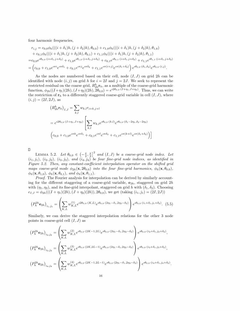
Lemma 5.2. Let θ0,0 ∈(−π

2 , π2

]2 and (I, J) be a coarse-grid node index. Let(i1, j1), (i2, j2), (i3, j3), and (i4, j4) be four fine-grid node indices, as identified inFigure 5.2. Then, any constant-coefficient interpolation operator on the shifted gridmaps coarse-grid mode φ2h(x, 2θ0,0) into the four fine-grid harmonics, φh(x, θ0,0),φh(x, θ1,0), φh(x, θ0,1), and φh(x, θ1,1).

Proof. The Fourier analysis for interpolation can be derived by similarly account-ing for the different staggering of a coarse-grid variable, e2h, staggered on grid 2hwith (η1, η2), and its fine-grid interpolant, staggered on grid h with (δ1, δ2). ChoosingeI,J = φ2h(((I + η1)(2h), (J + η2)(2h)), 2θ0,0), we get (taking (i1, j1) = (2I, 2J))

(P 2h

h e2h

)i1,j1

=

∑K,L

w(1)K,Leı2θ0,0·(K,L)eıθ0,0·(2η1−δ1,2η2−δ2)

eıθ0,0·(i1+δ1,j1+δ2). (5.5)

Similarly, we can derive the staggered interpolation relations for the other 3 nodepoints in coarse-grid cell (I, J) as

(P 2h

h e2h

)i2,j2

=

∑K,L

w(2)K,Leıθ0,0·(2K−1,2L)eıθ0,0·(2η1−δ1,2η2−δ2)

eıθ0,0·(i2+δ1,j2+δ2),

(P 2h

h e2h

)i3,j3

=

∑K,L

w(3)K,Leıθ0,0·(2K,2L−1)eıθ0,0·(2η1−δ1,2η2−δ2)

eıθ0,0·(i3+δ1,j3+δ2),

(P 2h

h e2h

)i4,j4

=

∑K,L

w(4)K,Leıθ0,0·(2K−1,2L−1)eıθ0,0·(2η1−δ1,2η2−δ2)

eıθ0,0·(i4+δ1,j4+δ2).

16

Making the ansatz that P 2hh e2h can be written as a linear combination of the four

Fourier harmonics, now on the shifted grid, we have(P 2h

h e2h

)i,j

= c0,0eıθ0,0·(i+δ1,j+δ2) + c1,0e

ıθ1,0·(i+δ1,j+δ2)

+ c0,1eıθ0,1·(i+δ1,j+δ2) + c1,1e

ıθ1,1·(i+δ1,j+δ2)

=(c0,0 + c1,0e

ıπ(i+δ1) + c0,1eıπ(j+δ2) + c1,1e

ıπ(i+j+δ1+δ2))

eıθ0,0·(i+δ1,j+δ2).

Equating terms for (i1, j1) = (2I, 2J) gives

c0,0 + c1,0eıπδ1 + c0,1e

ıπδ2 + c1,1eıπ(δ1+δ2) = c1(θ0,0),

for c1(θ0,0) given by the expression in Equation (5.5). With similar equations for theother interpolation nodes, we have

c0,0

c1,0eıπδ1

c0,1eıπδ2

c1,1eıπ(δ1+δ2)

= ε

1 1 1 11 −1 1 −11 1 −1 −11 −1 −1 1

∑K,L w

(1)K,Leı2θ0,0·(K,L)∑

K,L w(2)K,Leıθ0,0·(2K−1,2L)∑

K,L w(3)K,Leıθ0,0·(2K,2L−1)∑

K,L w(4)K,Leıθ0,0·(2K−1,2L−1)

,

with ε = eıθ0,0·(2η1−δ1,2η2−δ2)/4.

6. Numerical Examples. In this section, we give several smoothing and two-grid LFA estimates for systems of PDEs within the framework of multiplicative col-lective smoothers of Vanka-type. These smoothers, which explicitly deal with thelarge nullspaces that appear, are the only collective smoothers that give satisfactoryperformance for the operators of interest. We do not investigate the impact of theordering of the cells in the present paper and stay with a lexicographical ordering ofthe relaxation subsets.

To take LFA from its infinite-grid setting and get a predictive analysis tool, weneed to introduce a second discretization into the analysis, going from a continuousparameter, θ0,0, to a discrete mesh in θ0,0, upon which a convergence prediction canbe made. Thus, the results presented here have two step-size parameters: h, thespatial grid size, which is directly reflected in the coefficients of the discrete operatorsto which we apply LFA, and hθ, the mesh size for the discrete lattice of θ used tomake a quantitative prediction based on LFA.

A discrete set of the 4 × 4 Fourier blocks is then analyzed, corresponding to adiscrete choice of angles, θ0,0 ∈

(−π

2 , π2

]2, given by a tensor product of an equallyspaced mesh over the interval of length π with itself, with mesh-spacing hθ. Becausethe infinite-grid fine-grid and coarse-grid operators, Ah and B2h, are often singular,with the constant functions, φh(x, (0, 0)) and φ2h(x, (0, 0)), in their nullspaces, wechoose the mesh in θ0,0 so that θ0,0 = (0, 0) does not appear. A prediction of theperformance of the multigrid algorithm is made by measuring the largest eigenvalueof the transformed operators over this discrete space. All of the numbers quoted hereresult from this process, for h = 1

64 and hθ = π32 . The impact of finer meshes in either

space or Fourier frequency was negligible in the examples considered here.

6.1. The grad-div and the curl-curl operators. We first consider the dis-cretization of the gradient-divergence and the curl-curl equations, (2.1) and (2.2),respectively. As the stencils, multigrid methods, and smoothers, as well as their LFA

17

performance estimates are very similar for the two equations, we discuss them in onesection.

For the grad-div equation (2.1), we use first-order Raviart-Thomas (face) elementsfor the vector field U = (u, v)T , as already discussed in Section 2.2. The discretedegrees of freedom for this discretization are the values of u at the midpoints of meshedges that are parallel to the y-axis, and the values of v at the midpoint of mesh edgesthat are parallel to the x-axis. The resulting stencil, for u, reads, 1 −1

−1 2 −1−1 1

h

.

The contribution of the mass matrix is added, in the form of a one-dimensional addi-tion [h2/6 2h2/3 h2/6], with the central stencil element incremented by 2h2/3. Theresulting, rotated, stencil for the v components is similar.

As mentioned earlier, we choose the Nedelec edge elements [35] to discretize theweak curl-curl operator in (2.2), for unknown U = (u, v)T . The resulting stencil forthe u-component is

−1−1 1

21 −1−1

h

,

while, for v, we find an identical, but rotated, stencil. It is clear that the resultingstencils for the grad-div and curl-curl operators are identical, but rotated. So, wefocus on the discussion of the smoother for grad-div, as the one for curl-curl is similarand produces identical LFA results.

The overlapping smoother, in particular for the grad-div operator, was proposedin [1,2], where the degrees of freedom along the faces (edges) adjacent to a node werechosen to be relaxed simultaneously, see Figure 2.2. We refer to this as a node-wisesmoothing procedure.

We choose Si,j = ui,j− 12, ui,j+ 1

2, vi− 1

2 ,j , vi+ 12 ,j, and introduce in the local sys-

tem for smoothing the Fourier expansions for the errors in u and v, before relaxation,αueiθ·x/h, αveiθ·x/h, after the first correction, α′

ueiθ·x/h, α′veiθ·x/h, and after the sec-

ond correction, α′′ueiθ·x/h, α′′

veiθ·x/h as in Section 3. We can then write the updateequations in terms of the Fourier coefficients:

2h2

3 +2λ 0 λ −λ

0 2h2

3 +2λ −λ λ

λ −λ 2h2

3 +2λ 0−λ λ 0 2h2

3 +2λ

δui,j+ 12

δui,j− 12

δvi+ 12 ,j

δvi− 12 ,j

=

rui,j+ 1

2

rui,j− 1

2

rvi+ 1

2 ,j

rvi− 1

2 ,j

,

and convert this system into a system for α′′u, α′′

v , α′u, α′

v in terms of αu and αv, asexplained for Equation (4.1).

In the numerical LFA smoothing and two-grid experiments here, we vary thetransfer operators in the algorithms. We compare the usual six-point restriction op-erators, based on the fine grid residuals at the six nearest fine grid locations of thecorresponding unknown, with the two-point restriction operator. These operators are

18

dictated by the staggered arrangement of the unknowns. For the prolongation oper-ators we compare the transpose of the six-point restriction, i.e., the six-point inter-polation, with a twelve-point interpolation and a two-point interpolation. We denotethese transfer operators by 6r, 2r, 6p, 12p and 2p, respectively. See [36] or [42, §8.7.1]for details on these transfer operators. In the experiments, we fix the smoother tobe the lexicographical AFW smoother; the corresponding smoothing factor, basedon one smoothing iteration, is µ = 0.44. Further, the Galerkin coarse-grid operatoris chosen. Table 6.1 presents the corresponding two-grid LFA results. Results hereare shown for the grad-div (and curl-curl) parameter a = 106. However, for valuesof a ranging from 106 to O(1), we find identical LFA results; that is, no sensitivityto the value of the parameter a is observed. The results in Table 6.1, however, dodemonstrate a sensitivity to the choice of transfer operators, as with the two-pointrestriction operator even divergence of the solver is observed.

Table 6.1Two-grid LFA factors for different sets of transfer operators. Grad-div and curl-curl results

with a multiplicative AFW smoother.

restriction prolongation ρ2g , (1, 1)− cycle

6r 6p 0.1346r 12p 0.1342r 6p DIV6r 2p 0.53

The algorithm with the commonly chosen six-point transfer operators, however,shows an excellent two-grid factor for these problems. Very similar results are ob-tained with finite difference multigrid experiments for the grad-div operator in [20].These results can be labeled textbook multigrid efficiency, and an increasing numberof smoothing steps further decreases the two-grid factors. LFA smoothing analy-sis, as well as actual numerical multigrid experiments, indicate that an element-wisemultiplicative smoothing method, updating unknowns around the element center si-multaneously, does not provide any smoothing for this type of problem.

6.2. Stokes Equations. For the Taylor-Hood (Q2-Q1) elements on quadrilat-eral grids, there are many possible collections of unknowns that can be used to definethe relaxation subsets, Si,j . Vanka’s original choice for the staggered finite-differencediscretization of the Stokes equations [43] can be viewed both as being an element-wisechoice, as each relaxation subset consisted of the four velocity unknowns and singlepressure unknown on each grid cell, and also as being a pressure-wise choice, as theserelaxation subsets also correspond to the complete set of velocities that appear in thedivergence equation at a given pressure node plus that pressure node itself. For thisfinite-element discretization, however, the element-wise and pressure-wise relaxationsubsets are distinct. Further choices are also possible, such as the larger collectionsanalyzed in [32]. As first noted (without explanation) in [28], difficulties arise in usingelement-wise smoothing for the Taylor-Hood discretization. LFA confirms this, withsubstantial under-relaxation necessary to achieve a smoothing factor that is less thanone. For this reason, we focus here on the pressure-wise smoothing algorithm.

Table 6.2 displays both two-grid LFA convergence factors, ρ2g, and LFA smooth-ing factors, µ, for the full Vanka smoother using pressure-wise relaxation. Two typesof under-relaxation are considered: under-relaxation on only the velocities (as firstsuggested by Vanka [43]) and full under-relaxation, where the corrections to velocities

19

Velocity under-relaxation Full under-relaxationω ρ2g µ ρ2g µ1.0 0.77 0.76 0.77 0.760.9 0.67 0.74 0.58 0.670.8 0.58 0.71 0.43 0.610.7 0.48 0.68 0.37 0.600.6 0.38 0.65 0.45 0.670.5 0.36 0.60 0.54 0.74

Table 6.2Two-grid LFA convergence factors, ρ2g, and smoothing factors, µ, for the full Vanka smoother

for the Q2-Q1 discretization of Stokes with pressure-wise relaxation groups. In the left two columns,under-relaxation is used only on the velocity variables, while it is used on all variables (with thesame under-relaxation parameter) in the right two columns.

Fig. 6.1. At left, the amplification factor for the full pressure-wise Vanka smoother with nounder-relaxation for the Q2-Q1 discretization of the Stokes equations on a mesh with h = 1

64, as a

function of the Fourier mode, θ. At right, the spectrum of the two-grid error-propagation operatorusing this smoother with biquadratic interpolation for the velocities and bilinear interpolation forthe pressure.

and pressure are weighted equally. Both types of under-relaxation are shown to yieldsignificant improvement in both the smoothing and two-grid convergence factors. Fig-ures 6.1 and 6.2 depict the amplification factors for relaxation as a function of theFourier mode and the spectrum of the two-grid operator (sampled on a 64× 64 meshin the Fourier domain

[−π

2 , 3π2

]2) for no under-relaxation (in Fig. 6.1), and under-relaxation in velocity only with a factor of ω = 0.5 (in Fig. 6.2). Note that in theunder-relaxed case, the amplification factor near (π, π) is greater than 0.5; however,in this case, the reduction of error in the Fourier modes with frequencies near (π, π)by two steps of relaxation is in balance with the reduction in the smooth modes by thecoarse-grid correction process, leading to a much more efficient cycle than is achievedwith no weighting of the relaxation process.

Because of the expense of inverting the full velocity submatrix associated withthe relaxation subsets, a cheaper alternative to the full Vanka smoother using onlythe diagonal of this matrix is often considered [28, 31]. Table 6.3 gives two-grid LFAconvergence factors, ρ2g, and smoothing factors, µ, for this variant, known as thediagonal Vanka smoother. Here, we see that without under-relaxation, the smootheris mildly divergent; however, under-relaxation quickly resolves this and leads to a

20

Fig. 6.2. At left, the amplification factor for the full pressure-wise Vanka smoother with under-relaxation with parameter ω = 0.5 used for the velocities only with the Q2-Q1 discretization of theStokes equations on a mesh with h = 1

64, as a function of the Fourier mode, θ. At right, the spectrum

of the two-grid error-propagation operator using this smoother with biquadratic interpolation for thevelocities and bilinear interpolation for pressure.

Velocity under-relaxation Full under-relaxationω ρ2g µ ρ2g µ1.0 1.41 1.22 1.41 1.220.9 1.10 1.08 0.71 0.890.8 0.83 0.95 0.52 0.750.7 0.59 0.84 0.56 0.700.6 0.56 0.77 0.61 0.740.5 0.61 0.78 0.64 0.78

Table 6.3Two-grid LFA convergence factors, ρ2g, and smoothing factors, µ, for the diagonal Vanka

smoother for the Q2-Q1 discretization of Stokes with pressure-wise relaxation groups. In the lefttwo columns, under-relaxation is used only on the velocity variables, while it is used on all variables(with the same under-relaxation parameter) in the right two columns.

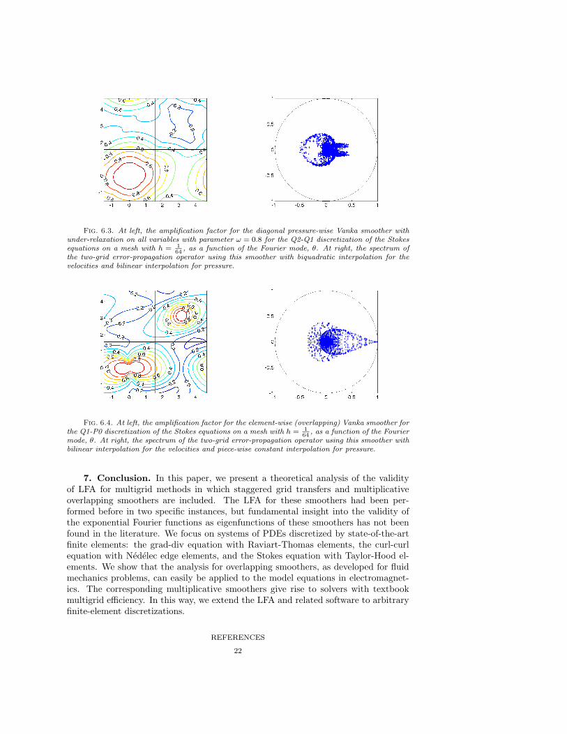
smoother that is much less expensive than, but also less effective than the full Vankasmoother. The amplification factor for this smoother and the spectrum of the two-grid iteration matrix using under-relaxation on all variables with parameter ω = 0.8are shown in Figure 6.3.

If we ignore the inf-sup condition (2.7) when discretizing Equations (2.5) and(2.6), one appealing discretization would be to represent the velocities by bilinearbasis functions and pressure as a piece-wise constant function on each element. Whileit is well-known that such an approach (without the addition of a stabilization term)sacrifices significant accuracy in the resulting solution [16,18], it is equally importantto note the difficulty in designing an efficient solver for this discretization. Figure 6.4shows the amplification factor for element-wise Vanka smoothing for this discretiza-tion (which is, in this case, the same as the pressure-wise smoother) at left, andthe spectrum of the two-grid error-propagation operator for a (1,1)-cycle at right.Adding under-relaxation to the velocities has little effect on these results, with anLFA smoothing factor of 0.995 for ω = 0.6, 0.7, 0.8, 0.9, and 1.0. Of particular inter-est is the large amplification factor associated with the Fourier mode at (π, π), whichis also the same mode that leads to the instability in the discretization.

21

Fig. 6.3. At left, the amplification factor for the diagonal pressure-wise Vanka smoother withunder-relaxation on all variables with parameter ω = 0.8 for the Q2-Q1 discretization of the Stokesequations on a mesh with h = 1

64, as a function of the Fourier mode, θ. At right, the spectrum of

the two-grid error-propagation operator using this smoother with biquadratic interpolation for thevelocities and bilinear interpolation for pressure.

Fig. 6.4. At left, the amplification factor for the element-wise (overlapping) Vanka smoother forthe Q1-P0 discretization of the Stokes equations on a mesh with h = 1

64, as a function of the Fourier

mode, θ. At right, the spectrum of the two-grid error-propagation operator using this smoother withbilinear interpolation for the velocities and piece-wise constant interpolation for pressure.

7. Conclusion. In this paper, we present a theoretical analysis of the validityof LFA for multigrid methods in which staggered grid transfers and multiplicativeoverlapping smoothers are included. The LFA for these smoothers had been per-formed before in two specific instances, but fundamental insight into the validity ofthe exponential Fourier functions as eigenfunctions of these smoothers has not beenfound in the literature. We focus on systems of PDEs discretized by state-of-the-artfinite elements: the grad-div equation with Raviart-Thomas elements, the curl-curlequation with Nedelec edge elements, and the Stokes equation with Taylor-Hood el-ements. We show that the analysis for overlapping smoothers, as developed for fluidmechanics problems, can easily be applied to the model equations in electromagnet-ics. The corresponding multiplicative smoothers give rise to solvers with textbookmultigrid efficiency. In this way, we extend the LFA and related software to arbitraryfinite-element discretizations.

REFERENCES

22

[1] D. Arnold, R. Falk, and R. Winther, Preconditioning in H(div) and applications, Math.Comp., 66 (1997), pp. 957–984.

[2] , Multigrid in H(div) and H(curl), Numer. Math., 85 (2000), pp. 197–217.[3] P. B. Bochev, C. J. Garasi, J. J. Hu, A. C. Robinson, and R. S. Tuminaro, An improved

algebraic multigrid method for solving Maxwell’s equations, Siam. J. Sci. Comput., 25(2003), pp. 623–642.

[4] T. Boonen, J. V. lent, and S. Vandewalle, Local Fourier analysis of multigrid for thecurl-curl equation, SIAM J. Sci. Comput., 30 (2008), pp. 1730–1755.

[5] A. Borzı, High-order discretization and multigrid solution of elliptic nonlinear constrainedoptimal control problems, J. Comput. Appl. Math., 200 (2007), pp. 67–85.

[6] D. Braess, Finite Elements, Cambridge University Press, Cambridge, 2001. Second Edition.[7] D. Braess and R. Sarazin, An efficient smoother for the Stokes problem., Appl. Numer.

Math., 23 (1997), pp. 3–20.[8] J. H. Bramble, J. E. Pasciak, J. Wang, and J. Xu, Convergence estimates for multigrid

algorithms without regularity assumptions, Math. Comp., 57 (1991), pp. 23–45.[9] A. Brandt, Multi–level adaptive solutions to boundary–value problems, Math. Comp., 31

(1977), pp. 333–390.[10] , Multigrid techniques: 1984 guide with applications to fluid dynamics, GMD–Studien

Nr. 85, Gesellschaft fur Mathematik und Datenverarbeitung, St. Augustin, 1984.[11] A. Brandt and N. Dinar, Multigrid solutions to elliptic flow problems, in Numerical Methods

for Partial Differential Equations, S. Parter, ed., Academic Press, New York, 1979, pp. 53–147.

[12] S. Brenner and L. Scott, The mathematical theory of finite element methods, vol. 15 ofTexts in Applied Mathematics, Springer-Verlag, New York, 1994.

[13] M. Brezina, A. Cleary, R. Falgout, V. Henson, J. Jones, T. Manteuffel, S. McCormick,and J. Ruge, Algebraic multigrid based on element interpolation (AMGe), SIAM J. Sci.Comput., 22 (2000), pp. 1570–1592.

[14] F. Brezzi and M. Fortin, Mixed and hybrid finite element methods, vol. 15 of Springer Seriesin Computational Mathematics, Springer-Verlag, New York, 1991.

[15] T. Chartier, R. Falgout, V. Henson, J. Jones, T. Manteuffel, S. McCormick, J. Ruge,and P. Vassilevski, Spectral element agglomerate AMGe, in Domain decomposition meth-ods in science and engineering XVI, vol. 55 of Lect. Notes Comput. Sci. Eng., Springer,Berlin, 2007, pp. 513–521.

[16] H. Elman, D. Silvester, and A. Wathen, Finite elements and fast iterative solvers: withapplications in incompressible fluid dynamics, Numerical Mathematics and Scientific Com-putation, Oxford University Press, New York, 2005.

[17] R. D. Falgout, P. S. Vassilevski, and L. T. Zikatanov, On two-grid convergence estimates,Numer. Linear Alg. Appl., 12 (2005), pp. 471–494. Also available as LLNL technical reportUCRL-JC-150807.

[18] M. Fortin, Old and new finite elements for incompressible flows, Internat. J. Numer. MethodsFluids, 1 (1981), pp. 347–364.

[19] F. Gaspar, J. Gracia, and F. Lisbona, Fourier analysis for multigrid methods on triangulargrids, SIAM Journal on Scientific Computing, 31 (2009), pp. 2081–2102.

[20] F. J. Gaspar, J. L. Gracia, F. J. Lisbona, and C. W. Oosterlee, Distributive smoothers inmultigrid for problems with dominating grad-div operators, Numer. Linear Algebra Appl.,15 (2008), pp. 661–683.

[21] V. Girault and P.-A. Raviart, Finite element approximation of the Navier-Stokes equations,vol. 749 of Lecture Notes in Mathematics, Springer-Verlag, Berlin, 1979.

[22] W. Hackbusch, Convergence of multi–grid iterations applied to difference equations, Math.Comp., 34 (1980), pp. 425–440.

[23] P. W. Hemker, W. Hoffmann, and M. H. van Raalte, Fourier two-level analysis for discon-tinuous Galerkin discretization with linear elements, Numer. Linear Alg. Appl., 11 (2004),pp. 473–491.

[24] R. Hiptmair, Multigrid method for H(div) in three dimensions, Electron. Trans. Numer. Anal.,6 (1997), pp. 133–152.

[25] , Multigrid method for Maxwell’s equations, SIAM J. Numer. Anal., 36 (1999), pp. 204–225.

[26] R. Hiptmair and R. H. W. Hoppe, Multilevel methods for mixed finite elements in threedimensions, Numer. Math., 82 (1999), pp. 253–279.

[27] J. Hu, R. Tuminaro, P. Bochev, C. Garasi, and A. Robinson, Toward an h-independentalgebraic multigrid method for Maxwell’s equations, SIAM J. Sci. Comput., 27 (2006),pp. 1669–1688.

23

[28] V. John and G. Matthies, Higher-order finite element discretizations in a benchmark problemfor incompressible flows, International Journal For Numerical Methods In Fluids, 37 (2001),pp. 885–903.

[29] V. John and L. Tobiska, Numerical performance of smoothers in coupled multigrid meth-ods for the parallel solution of the incompressible Navier-Stokes equations, InternationalJournal For Numerical Methods In Fluids, 33 (2000), pp. 453–473.

[30] T. V. Kolev and P. S. Vassilevski, AMG by element agglomeration and constrained energyminimization interpolation, Numer. Linear Algebra Appl., 13 (2006), pp. 771–788.

[31] M. Larin and A. Reusken, A comparative study of efficient iterative solvers for generalizedStokes equations, Numer. Linear Algebra Appl., 15 (2008), pp. 13–34.

[32] S. Manservisi, Numerical analysis of Vanka-type solvers for steady Stokes and Navier-Stokesflows, SIAM J. Numer. Anal., 44 (2006), pp. 2025–2056.

[33] S. F. McCormick, An algebraic interpretation of multigrid methods, SIAM J. Numer. Anal.,19 (1982), pp. 548–560.

[34] J. Molenaar, A two-grid analysis of the combination of mixed finite elements and Vanka-typerelaxation, in Multigrid Methods III, W. Hackbusch and U. Trottenberg, eds., vol. 98 ofInternational Series of Numerical Mathematics, Basel, 1991, Birkhauser, pp. 313–324.

[35] J.-C. Nedelec, Mixed finite elements in R3, Numer. Math., 35 (1980), pp. 315–341.[36] A. Niestegge and K. Witsch, Analysis of a multigrid Stokes solver, Appl. Math. Comput.,

35 (1990), pp. 291–303.[37] P.-A. Raviart and J. M. Thomas, A mixed finite element method for 2nd order elliptic

problems, in Mathematical aspects of finite element methods (Proc. Conf., Consiglio Naz.delle Ricerche (C.N.R.), Rome, 1975), Springer, Berlin, 1977, pp. 292–315. Lecture Notesin Math., Vol. 606.

[38] S. Reitzinger and J. Schoberl, An algebraic multigrid method for finite element discretiza-tions with edge elements, Numer. Linear Alg. Appl., 9 (2002), pp. 223–238.

[39] J. Schoberl and W. Zulehner, On Schwarz-type smoothers for saddle point problems, Numer.Math., 95 (2003), pp. 377–399.

[40] S. Sivaloganathan, The use of local mode analysis in the design and comparison of multigridmethods, Comput. Phys. Commun., 65 (1991), pp. 246–252.

[41] K. Stuben and U. Trottenberg, Multigrid methods: Fundamental algorithms, model problemanalysis and applications, in Multigrid Methods, W. Hackbusch and U. Trottenberg, eds.,vol. 960 of Lecture Notes in Mathematics, Berlin, 1982, Springer–Verlag, pp. 1–176.

[42] U. Trottenberg, C. W. Oosterlee, and A. Schuller, Multigrid, Academic Press, London,2001.

[43] S. P. Vanka, Block-implicit multigrid solution of Navier-Stokes equations in primitive vari-ables, J. Comput. Phys., 65 (1986), pp. 138–158.

[44] P. Vassilevski, Sparse matrix element topology with application to AMG(e) and precondi-tioning, Numer. Linear Alg. Appl., 9 (2002), pp. 429–444. Preconditioned robust iterativesolution methods, PRISM ’01 (Nijmegen).

[45] P. S. Vassilevski and J. P. Wang, Multilevel iterative methods for mixed finite elementdiscretizations of elliptic problems, Numer. Math., 63 (1992), pp. 503–520.

[46] R. Wienands and W. Joppich, Practical Fourier analysis for multigrid methods, vol. 4 ofNumerical Insights, Chapman & Hall/CRC, Boca Raton, FL, 2005. With 1 CD-ROM(Windows and UNIX).

[47] R. Wienands, C. W. Oosterlee, and T. Washio, Fourier analysis of GMRES(m) precondi-tioned by multigrid, SIAM J. Sci. Comput., 22 (2000), pp. 582–603.

[48] G. Wittum, On the robustness of ILU–smoothing, SIAM J. Sci. Stat. Comput., 10 (1989),pp. 699–717.

[49] H. Wobker and S. Turek, Numerical studies of Vanka-type smoothers in computational solidmechanics, Adv. Appl. Math. Mech., 1 (2009), pp. 29–55.

[50] I. Yavneh, On red-black SOR smoothing in multigrid, SIAM J. Sci. Comput., 17 (1996),pp. 180–192.

[51] G. Zhou and S. R. Fulton, Fourier analysis of multigrid methods on hexagonal grids, SIAMJournal on Scientific Computing, 31 (2009), pp. 1518–1538.

[52] H. bin Zubair, C. Oosterlee, and R. Wienands, Multigrid for high-dimensional ellipticpartial differential equations on non-equidistant grids, SIAM J. Sci. Comput., 29 (2007),pp. 1613–1636.

24