A low order Galerkin finite element method for the Navier–Stokes equations of steady incompressible flow: a stabilization issue and iterative methods Maxim A. Olshanskii Department of Mechanics and Mathematics, Moscow State University, Moscow 119899, Russia Received 25 May 2001; received in revised form 10 June 2002 Abstract A Galerkin finite element method is considered to approximate the incompressible Navier–Stokes equations together with iterative methods to solve a resulting system of algebraic equations. This system couples velocity and pressure unknowns, thus requiring a special technique for handling. We consider the Navier–Stokes equations in velocity–– kinematic pressure variables as well as in velocity––Bernoulli pressure variables. The latter leads to the rotation form of nonlinear terms. This form of the equations plays an important role in our studies. A consistent stabilization method is considered from a new view point. Theory and numerical results in the paper address both the accuracy of the discrete solutions and the effectiveness of solvers and a mutual interplay between these issues when particular stabilization techniques are applied. Ó 2002 Published by Elsevier Science B.V. Keywords: Navier–Stokes equations; Finite elements; Stabilized method; Oseen problem; Iterative methods 1. Introduction In this paper we consider the steady incompressible Navier–Stokes equations (1). Typically to solve a computational fluid dynamic problem a researcher is free to build a method in many ways by choosing different discretization techniques, solvers for resulting discrete system, and setting a lot of parameters to some particular values. A lot of tools are available to treat the problem (1) numerically. For example one can choose a method from a family of finite differences, finite elements or finite volumes. Further a pseudotime stepping or another iterative solver for the nonlinear problem can be applied to find time-in- dependent solutions. One can try to reformulate the original continuous problem and doing that to obtain discrete systems with different properties. These and many other particular ingredients can be put together in many ways and this may crucially influence the quality of a final solution obtained as well as the total Comput. Methods Appl. Mech. Engrg. 191 (2002) 5515–5536 www.elsevier.com/locate/cma E-mail address: [email protected](M.A. Olshanskii). 0045-7825/02/$ - see front matter Ó 2002 Published by Elsevier Science B.V. PII:S0045-7825(02)00513-3
Transcript
A low order Galerkin finite element method for theNavier–Stokes equations of steady incompressible flow:
a stabilization issue and iterative methods
Maxim A. Olshanskii
Department of Mechanics and Mathematics, Moscow State University, Moscow 119899, Russia
Received 25 May 2001; received in revised form 10 June 2002
Abstract
AGalerkin finite element method is considered to approximate the incompressible Navier–Stokes equations together
with iterative methods to solve a resulting system of algebraic equations. This system couples velocity and pressure
unknowns, thus requiring a special technique for handling. We consider the Navier–Stokes equations in velocity––
kinematic pressure variables as well as in velocity––Bernoulli pressure variables. The latter leads to the rotation form of
nonlinear terms. This form of the equations plays an important role in our studies. A consistent stabilization method is
considered from a new view point. Theory and numerical results in the paper address both the accuracy of the discrete
solutions and the effectiveness of solvers and a mutual interplay between these issues when particular stabilization
In this paper we consider the steady incompressible Navier–Stokes equations (1). Typically to solve a
computational fluid dynamic problem a researcher is free to build a method in many ways by choosing
different discretization techniques, solvers for resulting discrete system, and setting a lot of parameters to
some particular values. A lot of tools are available to treat the problem (1) numerically. For example onecan choose a method from a family of finite differences, finite elements or finite volumes. Further a
pseudotime stepping or another iterative solver for the nonlinear problem can be applied to find time-in-
dependent solutions. One can try to reformulate the original continuous problem and doing that to obtain
discrete systems with different properties. These and many other particular ingredients can be put together
in many ways and this may crucially influence the quality of a final solution obtained as well as the total
CPU time of computations. Although the ‘‘best’’ method, if it exists, seems to be problem dependent, areasonable objective is a method, which is able to solve a possibly widest class of problems efficiently, i.e.
with acceptable guaranteed accuracy and CPU time. Recently a considerable effort has been made to
compare the performance of various tools for simulating flow problems (see, e.g., [14,27,28,36,42], and
monograph [44]) and to derive optimal schemes. Nevertheless a demand for predictable, robust, and effi-
cient solvers/methods still exists. A good candidate for such a method is a finite element method
for the ‘‘true’’ mixed formulation of the Navier–Stokes equations, since applied properly it has good
stability properties and gives the possibility of the rigorous error control (e.g., [41]). However, the method
is efficient only if the resulting discrete systems, having a quite complicated structure, can be solved effi-ciently.
The present paper is concerned with both the accuracy of the FE method and the numerical performance
of linear algebra tools applied here to solve discrete systems. We are in no way exhaustive in these topics
and concentrate further on techniques and results which are new, mentioning briefly those which are
standard. The total machinery applied to treat the problem consists of the following basic tools:
(a) A low order FE method (P1isoP2/P0 in experiments). Two types of consistent stabilization are addi-
tionally considered. One is the SUPG method, another one amounts in adding particular term derivedfrom the continuity equation to the momentum one.
(b) The fixed point or implicit backward Euler (BE) method to find a steady solution to a nonlinear prob-
lem.
(c) A block-triangular preconditioning combined with the BiCGstab iterations to solve the linearized
Navier–Stokes problem (of Oseen type).
(d) Geometric multi-grid methods to solve or to approximate subproblems for velocity and pressure, which
appear in item (c).
Details can be found in the next sections.
Non of the items (a)–(d) is absolutely new. Although the particular way of combining them is something
we do not find in the literature, similar ‘‘configurations’’ can be found in [44]. However, we emphasize in the
paper several ingredients which are new or not well studied, but were found to improve the overall per-
formance of the method. Referring to the remainder of the paper for details, we outline them briefly:
(a) The rotation form of the Navier–Stokes equations (2) is a starting point for FE approximation in some
experiments. It also appears to be useful for theoretical analysis of a solver performance. Where appro-priate we will compare the performance of the rotation form with more commonly used convection
form (1).
(b) A particular stabilization method is studied numerically and understood from the theoretical point of
view: An additional term, crdivu, resulting from the continuity equation is added to the momentumone. Early this term has appeared in residual-based stabilization methods (e.g., [17,33]), but its role
remained not very clear. We will see that the adding of this term intends to reduce the loss of accuracy,
which the discrete solution suffers for small viscosity values due to the presence of the first-order pres-
sure term (see Section 2.1). In the theory this effect does not depend on convection, however in exper-iments with a benchmark nonlinear problem (driven cavity), this stabilization was found to be
especially important, if calculations are based on the form of equations with Bernoulli (total) pressure
(2). We see the reason in the fact that for this problem the Bernoulli pressure appears to be more ‘‘sub-
stantial’’ variable compared to the kinematic pressure.
(c) Preconditioned iterations to solve the linearized Navier–Stokes problem. A specially designed precon-
ditioner is used in the iterations. Moreover we will see that the stabilization mentioned in item (b) is
important for a superior behavior of this linear solver.
Apart from the theory, numerical experiments for several problems are documented in detail. Oneproblem has analytical solution, another one is the driven-cavity problem for moderate and high Reynolds
numbers, the third one is ‘‘1:2’’ backward facing step problem with Re ¼ 150 and Re ¼ 800. Most im-portant results and conclusions are summarized in the final section.
2. The problem and FE method
Let X be a bounded polygonal domain in RN , N ¼ 2, 3. We consider the steady incompressible Navier–Stokes equations in the convection form: Find a vector function uðxÞ (velocity) and a scalar function pðxÞ(kinematic pressure) from
� mDuþ ðu � rÞuþrp ¼ f in X;
divu ¼ 0 in Xð1Þ
with given force field f and viscosity m > 0. Some boundary conditions should be additionally supplied (e.g.,for velocity or stress tensor, but not solely for pressure cf. [22]). Throughout this section we assume homo-
geneous Dirichlet boundary conditions: u ¼ 0 on oX.We also consider the rotation form of the Navier–Stokes problem:
� mDuþ ðcurluÞ � uþrP ¼ f in X;
divu ¼ 0 in X:ð2Þ
The equivalence of these two formulations follows from the relation
ðu � rÞu ¼ ðcurluÞ � uþ 12rðu2Þ ð3Þ
with u2 :¼ u21 þ � � � þ u2N . Thus the pressure distributions differ in these formulations. The Bernoulli pressureP in (2) and the kinematic pressure p in (1) are tied by
P ¼ p þ 12u2: ð4Þ
The velocity field recovered in (1) and (2) is the same.
Given conforming FE spaces Uh H10ðXÞ and Qh L02ðXÞ, the Galerkin FE discretization of (1) or (2) isstraightforward: Find fuh; phg 2 Uh � Qh from
mðruh;rvhÞ þ Nðuh; uh; vhÞ � ðph; divvhÞ þ ðqh; divuhÞ ¼ ðf; vhÞ 8vh 2 Uh; qh 2 Qh; ð5Þwhere Nða; u; vÞ is either ðða � rÞu; vÞ or ððcurlaÞ � u; vÞ, depending on a form of equations used. Contraryto continuous case different forms of the equations in the FE scheme (5) may give different velocities uh:
relation (3) does not hold on the FE level unless u2h 2 Qh, the latter is not the case for any standard Uh=Qh
FE pair. For the rotation form the conservation principle is readily fulfilled on a finite element level thanks
to the property of the vector product operation: Nðuh; uh; uhÞ ¼ 0, which implies
mkruhk2 ¼ ðf; uhÞ: ð6Þ
Here and further k � k denotes the L2 norm and krvk ¼ ðPN
i;j¼1 koui=oxjk2Þ1=2. For the convection form
conservation can be ensured by setting Nða; u; vÞ ¼ 1=2fðða � rÞu; vÞ � ðða � rÞv; uÞg, leading however toextra computations.
There are several critical issues associated with the Galerkin FE method. One is the compatibility of Uh
and Qh, i.e. the validation of the LBB (infsup) stability condition (see, e.g., [24]). LBB condition guarantees
that the FE velocity space is rich enough, comparing to FE pressure space, ensuring well-posedness and full
approximation order for the FE linear problem. In numerical experiments in the paper we used P1isoP2/P0
FE pair (piecewise-constant pressure and piecewise-linear continuous velocity on 2-times finer triangula-tion), which is LBB stable [24]: There exists mesh-independent constant lðXÞ, such that
infqh2Qh
supvh2Uh
ðqh; divvhÞkrvhkkqhk
¼ lh P lðXÞ > 0: ð7Þ
It is well known that the Galerkin FE method gives optimal convergence results for elliptic problems. Thus
for low order finite elements, which we used, theorem 4.2 from Chapter IV in [20] ensures Oðh2Þ asymptoticconvergence of ku� uhk and OðhÞ of kp � phk provided that some assumptions on regularity of u, p and Xare valid. However, if a continuous problem losses its ellipticity, as happens with (1) or (2) as m ! 0, theaccuracy of the FE solution may deteriorate and the asymptotic convergence may be feasible for very fine
meshes only. Therefore reasonable discrete solutions become available with a mesh, which resolve a stiff
physical behavior of a continuous solution. Such a mesh may be prohibitively fine for practical compu-tations, for this reason upwind, Petrov–Galerkin, or least-squares methods are popular, since they enhance
stability (ellipticity) of the discrete system, preserving (hopefully) approximation properties. In some nu-
merical experiments we will use the SUPG method. Additionally in the next section we go into some details
of what we call ‘‘rdiv’’-stabilization. Although this alteration of the basic Galerkin method (5) is not newand can be found in [13,17,33,46], we concentrate on this issue for the following reasons: Neither physical
nor numerical contents of it seems has been clearly understood; The cited references give different recipes
for choosing ‘‘optimal’’ parameter, leaving unclear whether this additional term plays a key role or is in-
troduced for technical reasons only; We will see in theory and numerical experiments a positive effect both
on solution accuracy and the solver performance; For the equations in the rotation form this stabilization
was found to be necessary already for driven cavity problem with Re ¼ 400.
2.1. »div––stabilization
Consider as a model the Stokes problem:
� mDuþrp ¼ f in X;
divu ¼ 0 in X:ð8Þ
The FE scheme for this problem reads: Find fuh; phg 2 Uh � Qh solving
mðruh;rvhÞ þ cðdivuh; divvhÞ þ ðph; divvhÞ � ðqh; divuhÞ ¼ ðf; vhÞ 8fvh; qhg 2 Uh � Qh: ð9ÞThe parameter cP 0 is a stabilization parameter, which role is underpined by the error estimate in thetheorem below and numerical experiments in Section 4. Since the term cðdivuh; divvhÞ in (9) can be viewedas adding the consistent term crdivu to the momentum equation in (8), we call (9) the rdiv -stabilizedscheme. Although this term is consistent for continuous equations, the finite element solution depends on a
value of c. As we will see, too large values of c ‘‘overstabilize’’ the problem and make corresponding linearalgebraic system poor conditioned. The question of an optimal c will be addressed further.
Theorem 1. Assume that Uh and Qh are such that lh from (7) is positive. Denote b ¼ maxfm; cg. The followingerror estimate holds
mkrðu� uhÞk2 þ ckdiv ðu� uhÞk2 þl2hbkp � phk2
6C inf/2Uh
mkrðu��
� /Þk2 þ c
�þ b
l2h
�kdiv ðu� /Þk2
�þ 1
binfw2Qh
kp � wk2�
ð10Þ
with some constant C > 0 independent of u, p, and all parameters of the problem.
Step 1 (stability estimate). First we show that for arbitrary feh; rhg from fUh � Qhg there exists a pairfvh; qhg such that
aðeh; rh; vh; qhÞP1
4jjjeh; rhjjj jjjvh; qhjjj: ð11Þ
Condition (7) enables us to consider zh 2 Uh such that krzhk ¼ krhk and ðrh; divzhÞP lhkrhkkrzhk: Thenan appropriate choice of fvh; qhg in (11) can be vh ¼ eh þ ðlh=2bÞzh, qh ¼ rh. Indeed, via Young�s inequalitywe get
aðeh; rh; eh; rhÞP mkrehk2 þ ckdivehk2;
aðeh; rh; zh; 0ÞPlh
2krhk2 �
m2
lhkrehk2 �
c2
lhkdivehk2:
We multiply the second inequality by lh=2b and add it to the first one. This leads to
a eh; rh; eh
�þ lh
2bzh; qh
�P
m2krehk2 þ
c2kdivehk2 þ
l2h4b
krhk2P1
2jjjeh; rhjjj2:
Now to prove inequality (11) we need to show
jjjvh; qhjjj6 2jjjeh; rhjjj:The latter is easy to see, thanks to the definition of qh ¼ rh and vh ¼ eh þ ðlh=2bÞzh, and
lh
2bzh; 0
��������
��������
��������2
¼ l2h4b2
ðmkrzhk2 þ ckdivzhk2Þ6l2h2b
krhk26 jjjeh; rhjjj2:
Step 2 (continuity estimate). From the Cauchy inequality we get for any fe; rg and fv; qg fromH10ðXÞ � L02
þ kqkkdivek6ffiffiffiffiffiffiffiffiffiffiffiffiffiffiffiffiffiffiffiffiffiffiffiffiffiffiffiffiffiffiffiffiffiffiffiffiffiffiffiffiffiffiffiffiffiffiffiffiffiffiffiffiffiffiffiffiffiffiffiffiffiffiffiffiffiffiffiffiffiffiffiffiffiffiffimkrek2 þ c þ b
l2h
� �kdivek2 þ 1
bkrk2
s ffiffiffiffiffiffiffiffiffiffiffiffiffiffiffiffiffiffiffiffiffiffiffiffiffiffiffiffiffiffiffiffiffiffiffiffiffiffiffiffiffiffiffiffiffiffiffiffiffiffiffiffiffiffiffiffiffiffiffiffiffiffiffiffiffi2ðmkrvk2 þ ckdivvk2Þ þ l2h
bkqk2
s
¼ffiffiffi2
pffiffiffiffiffiffiffiffiffiffiffiffiffiffiffiffiffiffiffiffiffiffiffiffiffiffiffiffiffiffiffiffiffiffiffiffiffiffiffiffiffiffiffiffiffiffiffiffiffiffiffiffiffiffiffiffiffiffiffiffiffiffiffiffiffiffiffiffiffiffiffiffiffiffiffimkrek2 þ c þ b
l2h
� �kdivek2 þ 1
bkrk2
sjjjv; qjjj ¼
ffiffiffi2
p‘ðe; rÞjjjv; qjjj: ð12Þ
Here we denote
‘ðe; rÞ ¼ffiffiffiffiffiffiffiffiffiffiffiffiffiffiffiffiffiffiffiffiffiffiffiffiffiffiffiffiffiffiffiffiffiffiffiffiffiffiffiffiffiffiffiffiffiffiffiffiffiffiffiffiffiffiffiffiffiffiffiffiffiffiffiffiffiffiffiffiffiffiffiffiffiffiffimkrek2 þ c þ b
l2h
� �kdivek2 þ 1
bkrk2
s:
Step 3. Let eh ¼ uh � /, rh ¼ ph � w and e ¼ u� /, r ¼ p � w for some arbitrary / 2 Uh and w 2 Qh: TheGalerkin orthogonality implies
Since / and w in the definition of e and r are arbitrary functions from Uh and Qh, we can take infimum in
the r.h.s. in (14) over these spaces. Therefore we arrive at (10) with C ¼ ð4ffiffiffi2
pþ 1Þ2 after squaring. �
The theorem can be applied to draw convergence estimates for a particular LBB-stable finite element
pair as in the example below.
Example 1. Assume the solution to the Stokes problem (8) is smooth enough and the mesh is quasi-regular,
then for P1isoP2/P0 finite elements we have
mkrðu� uhÞk2 þl2hbkp � phk26Ch2 b 1
��þ 1
l2h
�kuk2H2 þ
1
bkpk2H1
�: ð15Þ
To see the predicted effect of introducing c-term suppose that the problem (8) has a non-trivial continuouspressure solution (p 62 Qh) and suppose for a moment that u and p are independent of m, then for c ¼ 0 theestimate (15) ensures only
krðu� uhÞk6cðhÞm
; ð16Þ
while for c ¼ Oð1Þ
krðu� uhÞk6cðhÞffiffiffi
mp ; ð17Þ
where a constant cðhÞ depends on approximation properties of FE spaces and p, but not on m. Moreover forc ¼ Oð1Þ the following natural norm of the error
is controlled independently of m, although this norm becomes weak for velocity if m ! 0. Of course, in �real�problems both u and p are m-dependent, and therefore their norms involved in standard approximationestimates, say kukH2 and kpkH1 , can be m-dependent too. For the Navier–Stokes problem this dependence ishard to predict. A standard regularity theory for the equations suggests kukHk � kpkHk�1 . At the same time
theory from this section, in particular (16) and (17), is well supported by numerical experiments not only for
the Stokes problem, but also for the linearized Navier–Stokes problem. Experiments with nonlinear
problem also clearly show that rdiv-stabilization improves accuracy for carefully chosen parameter c.Example 1 illustrates that this stabilization intends to suppress instabilities induced by the pressure,
whenever kpkH1 is noticeable.The estimate (10) hints also the best choice of the stabilization parameter. Consider first the case when an
approximation of velocity is one degree larger than of pressure (e.g., P1isoP2–P0, non-conforming P1–P0,P2–P1 FE pairs), then a balance of the last two terms in (10) gives the choice c � lh for m6 lh and c ¼ 0otherwise. In the case of equal order approximation (e.g., P1isoP2–P1 FE pair) the best choice is c � lhh form6 lhh, however provided that the pressure is sufficiently smooth: kpkH2 is reasonably bounded. Numericalexperiments with P1isoP2–P0 FE pair in the paper confirm the above choice. For some simple domains
quite accurate estimates of lh are known (see [11]). Moreover numerical experiments in [11] show that lh
does not depend on the anisotropy of triangulation for P1isoP2–P0 elements, see [1] for the coverage of
The ‘‘new’’ term in (19) is evaluated element-wise for each element s of a triangulation Th. A parameterrðs; uhÞ is element and solution-dependent. Several recommendations can be found in literature for thechoice of rðs; uhÞ. The general idea is to add almost no additional stabilization terms in regions of smallmesh Reynolds numbers, hence to recover �optimal�Galerkin method by setting rðsÞ � 1 (or even rðsÞ ¼ 0)in these regions, but to add these terms in regions of large mesh Reynolds numbers. However, the particular
choice of rðs; uhÞ is still a matter of discussion. We use the one from [33] and [44], see also [34]:
rðs; uhÞ ¼ rhs
kukX
2Res
1þ Res; Res :¼
kukL2ðsÞhs
m: ð20Þ
This choice is provided by the minimization of an a priori error estimate for the discrete solution of (19) and
was successfully tested in many numerical experiments in [44].
In our experiments we take either r ¼ 0:2 or r ¼ 0, the latter means that no SUPG terms are added. Forisotropic meshes hs represents a diameter of element s. In the case of anisotropic meshes hs can be chosen as
an ‘‘effective’’ mesh size: An element diameter in a flow direction [18]. Another analysis for anisotropic grids
is found in [2].
Since we use piecewise-linear approximation for velocity and piecewise-constant for pressure, viscous and
pressure terms disappear from FE residual in (19) and the method amounts in addingP
s2Th rðs; uhÞðuh �ruh; uh � rvhÞs to momentum equations. If f 6¼ 0, then the extra f-dependent term is also added.In our numerical experiments SUPG method will be used for calculating high-Re flows and only with
convection form of equations.
3. Solvers
To illustrate ideas that are fairly standard we will occasionally use ‘‘continuous’’ notations in this sec-
tion. When details are important we will operate with matrices and vectors of nodal values. To solve
nonlinear problem the fix-point defect correction method is applied: Given iterate fum; pmg and relaxationparameter x > 0 find fumþ1; pmþ1g from
where Nðum; umÞ ¼ curlum � um or ¼ um � rum: For r > 0 the SUPG terms are also included to compute thedefect in (21). LNSðumÞ�1 is a solution operator to the linearized Navier–Stokes equations. This iterationsare quite robust for the problem in the convection form [44], especially if stabilizing terms are added.
However we found that for the rotation form iterations (21) are not so robust for small m. Thus in the case
of the rotation form we use implicit BE method. Then on every ‘‘time’’ step of BE one arrives at nonlinear
problem similar to (1) or (2) with additional reactive term ð1=dtÞu in the momentum equations. To solvethis new nonlinear problem we perform few iterations (21), taking velocity from the previous time as an
initial guess.
The linearized problem to be solved on each iteration (21) reads: Given um and resmu find fv; qg from
1
dtv� mDv� crdivvþ Nðum; vÞ þ rq ¼ resmu in X;
� divv ¼ �divum in X;
homogenuous b:c: on oX;
ð22Þ
where Nðum; vÞ ¼ curlum � v for the rotation form and Nðum; vÞ ¼ ðum � rÞv for the convection one. If theSUPG method is used for nonlinear problems, then the SUPG term is linearized in the natural way:P
s rðs; umÞðum � rvh; um � rwhÞs and included in the FE formulation of (22). This additional term is sym-
metric and non-negative.
Note that the linearization of equations in rotation form results in the 0-order term ðcurlumÞ � v in (22),comparing to the 1st-order of ðum � rÞv in convection form. In both cases the linearized equations preserveellipticity and conservation property (6).
3.1. Linear solver
Problem (22) is linear, however non-symmetric and of saddle-point type. Therefore a special technique is
required to treat it. To solve (22) we use coupled iterations, i.e. pressure and velocity are iterated together.
Several methods of this type can be found in the literature. Often direct multi-grid methods are used (e.g.[25,45,51,52]). Discussion of advantages and disadvantages of such methods and further references can be
found in [50]. Trying to avoid particular problems associated with building a multigrid for saddle-point
problem, more recently preconditioned methods based on outer–inner iteration, which have a long history
[4] for symmetric saddle-point problems, were adopted for non-symmetric ones (e.g., [8,16,37,43]). It is not
our intention here to compare these different approaches, see results of this type for symmetric case in [14].
Below we consider preconditioned method based on outer–inner iterations with particular attention to the
case of m ! 0.Let A and B be matrices stemming from a FE method applied to (22): For any basic nodal functions
wi;wj 2 Uh and /k 2 Qh the entries of matrices A and B are defined by
Ai;j ¼ mðrwj;rwiÞ þ cðdivwj; divwiÞ þ1
dtwj
�þ Nðum;wjÞ;wi
�þXs2Th
rðs; umÞðum � rwj; um � rwiÞs;
Bk;i ¼ �ðdivwi;/kÞ:
With these notations one has to solve the system of linear algebraic equations:
A BT
B 0
� �xy
� �¼ f
g
� �: ð23Þ
The spectrum of the matrix from (23) contains eigenvalues with both positive and negative real parts and its
condition number strongly depends on the mesh-size and m ([16,37,48]), leading to a poor conditioning ash ! 0 and/or m ! 0. Thus to solve (23) iteratively a preconditioning is highly desirable. Let AA be a pre-conditioner for A and SS a preconditioner for S, the Schur complement of the system:
Using a pattern from [30], the block triangular preconditioner for (23) is defined as
P�1 ¼ AA�1 AA�1BTSS�1
0 �SS�1
!: ð24Þ
If AA ¼ A and SS ¼ S, then a preconditioned Krylov subspace method for (23) will converge in at most twoiterations. Generally, we are looking for AA and SS to be close to A and S, but such that AA�1x and SS�1y can be‘‘easily’’ computed for given vectors x and y. Convergence analysis of the GMRES method with thispreconditioning is given in [30]. We use the BiCGstab method [47] to iterate the following preconditioned
system up to a desirable tolerance:
A BT
B 0
� �AA�1 AA�1BTSS�1
0 �SS�1
!xxyy
� �¼ f
g
� �: ð25Þ
Two essential ingredients: AA and SS are remaining to be defined. First let us consider the rotation form. Indoing this we use some ideas from [37,38]. AA is a preconditioner for the pure velocity problem. The con-tinuous counterpart of this problem reads
av� mDv� crdivvþ w� v ¼ r:h:s in X;
homogenuous b:c: on oXð26Þ
with w ¼ curlum, a ¼ 1=dt. Compared to the convection–diffusion vector problem that appears, if onelinearize the Navier–Stokes equations in convection form, Eq. (26) has 2nd-order and 0-order terms only.
This allows standard multi-grid components to work well and to solve a FE approximation of Eq. (26).
Multi-grid components include a block Jacobi or block Gauss–Seidel iteration as smoother. The robustnessof the multi-grid as a solver was proved in [38] for the case c ¼ 0. At the same time, if c ¼ Oð1Þ andm; a ! 0, the problem (26) has anisotropic diffusion terms and may have a large kernel in the limit casem ¼ 0 and a ¼ 0, therefore the performance of standard multi-grid tools deteriorates. Fortunately, as wewill see from numerical experiments, for the realistic values of m, a loss in convergence is not dramatic andwe have a hope that specially designed smoothing and prolongation operators can further improve the
situation. We summarize all these, saying that for AA�1 we take few V-cycles of the multi-grid method
applied to solve FE system approximating (26).
Demand for a preconditioner to the Schur complement S is the price we pay for the desire to solve ‘‘true’’coupled systems like (1) or (2), rather then to decouple somehow pressure from the original system [39].
Matrix S is a dense matrix: Most entries are non-zero and cannot be computed in a straightforward(economical) manner. Therefore, non-standard considerations have to be made to build SS. Below wepresent a particular choice of SS and some analysis aimed to predict the robustness of this choice follows. LetMp be a mass matrix for the pressure FE space and MMp its diagonal lumping, then
SS�1 ¼ ðm þ cÞMM�1p þ S0ðwÞ�1; ð27Þ
where S0ðwÞ :¼ BMMuðwÞ�1BT is a Schur complement of
MMuðwÞ BT
B 0
� �; where in two-dimensional case MMuðwÞ ¼ aMMu �MMw
u
MMwu aMMu
!; ð28Þ
MMu is a lumped velocity mass matrix and MMwu is a lumped mass-type matrix, corresponding to the
w-weighted scalar productR
X wðxÞuðxÞvðxÞdx. For further clarity we note that (28) can be viewed as thematrix of a discrete counterpart of the following reduced (m ¼ 0, c ¼ 0) problem Eq. (22):
homogenous b:c: for v � n on oX; n� normal vector to oX:
ð29Þ
In the three-dimensional case MMuðwÞ is a 3� 3 block matrix. The Schur complement S0ðwÞ of the reducedproblem is now a sparse matrix that mimics a mixed discretization for the pressure-Poisson problem.
Therefore, a multi-grid method is a good candidate to evaluate S0ðwÞ�1: In fact, few multi-grid V-cycles willsuffice for our needs.
Important to note that problem (29) (resp. (28)) can be ill-posed for a ¼ 0: Two decisions can be madefor small a. The first, which we commonly take, is to add S0ðwÞ�1 to (27) only if aP �aa. We take �aa ¼ 1 in theexperiments. However, if a ¼ 0 and c ¼ 0 the analysis in the next section predicts that artificial �aa � kwk is auseful choice for the case of a small viscosity. We will call SS with �aa––a modified Schur complement pre-conditioner.
For the Navier–Stokes equations in convection form the linearization leads to system (23). Now A standsfor a matrix corresponding to a discretization of the vector convection–diffusion problem (with the reactive
term and anisotropic diffusion):
av� mDv� crdivvþ ða � rÞv ¼ r:h:s in X;
homogenuous b:c: on oX;ð30Þ
with a ¼ um. If c ¼ 0, then the system (30) splits into two scalar convection–diffusion problems. For a FEapproximation of the latter multi-grid methods are known to be a good choice as solvers. We use a geo-
metric multi-grid method to build a preconditioner AA. Smoother, grid transfer operators, and coarse-grid matrices are the main ingredients to be defined. We found that for stabilized equations the appropriate
choice was standard (induced by the embeddings U2h Uh and P2h Ph) 1st-order projection and restric-tion, alternating Gauss-Seidel method with lexicographical ordering of unknowns as a smoother, and a FEapproximation of (30) on a coarse grid as the coarse-grid problem. For the coarse-grid problem we
found important to define SUPG stabilization parameters correspond to the coarse grid; for a similar
experience with a multi-grid method for convection–diffusion equations see [40]. For globally refined grids
multi-grid methods, e.g. V- and W-cycles for two-dimensional problems lead to optimal complexity,
however for locally refined grids special smoothing strategies should be used to retain optimal complexity
(see, [5]).
A proper preconditioner for the Schur complement S in the convection form is a challenging problem.Recently in [15,31,43] two types of preconditioners, which take the convection into account, were proposed.They were derived with assumptions on convection a to be a constant vector and boundary conditions to be
periodic. Both preconditioners require the construction of operators of the convection–diffusion type on the
discrete pressure space. For piecewise constant pressure this imposes certain difficulties. One possible way
to overcome them [49] is to consider a dual triangulation for the pressure by connecting the centroids of the
triangles in which pressure is defined. Then one can define piecewise linear and continuous pressure on the
dual triangulation. Avoiding additional implementation efforts, we alternatively set SS�1 ¼ ðm þ cÞMM�1p .
Numerical experiments from [31,43] show the advantage of their more sophisticated preconditioner for the
case of c ¼ 0, this modification can be especially useful for higher order pressure approximations.
3.2. Fourier analysis
This subsection gives an analysis that explains the advantage of the choice (27) of SS. We consider thetwo-dimensional periodic case and constant wðxÞ ¼ w 6¼ 0:
Let us evaluate the operator S on a given harmonic qðxÞ ¼ expðiðc; xÞÞ, where c; x 2 R2. First we have
rqðxÞ ¼ fic1 expðiðc; xÞÞ; ic2 expðiðc; xÞÞg:
Looking for u of the form u1 ¼ ik1 expðiðc; xÞÞ, u2 ¼ ik2 expðiðc; xÞÞ, we find from
� mDu1 � co
ox1
ou1ox1
�þ ou2
ox2
�þ au1 � wu2 ¼
oqðxÞox1
;
� mDu2 � co
ox2
ou1ox1
�þ ou2
ox2
�þ au2 þ wu1 ¼
oqðxÞox2
the coefficients
k1 ¼ða þ mjcj2 þ cc22Þc1 þ ðcc1c2 þ wÞc2
ða þ mjcj2cc21Þða þ mjcj2cc22Þ � c2c21c22 þ w2
;
k2 ¼ða þ mjcj2 þ cc21Þc2 � ðcc1c2 þ wÞc1
ða þ mjcj2cc21Þða þ mjcj2cc22Þ � c2c21c22 þ w2
:
Therefore,
S expðiðc; xÞÞ ¼ �divu ¼ ða þ mjcj2Þjcj2
ða þ mjcj2Þða þ ðm þ cÞjcj2Þ þ w2expðiðc; xÞÞ:
Let us consider the case of a ¼ 0. For a > 0 the condition number of the preconditioned system only improves
and m-independent estimates can be obtained (see relevant analysis for the case c ¼ 0 in [37]). For a ¼ 0 weomit S0ðwÞ�1 in SS�1 and for the preconditioned problem we have
SS�1S expðiðc; xÞÞ ¼ mðm þ cÞjcj4
mðm þ cÞjcj4 þ w2expðiðc; xÞÞ: ð31Þ
This results for fine enough mesh (jcj4 can be large) in
c ¼ Oð1Þ: condðSS�1SÞ � 1þOðm�1Þ; m ! 0; ð32Þ
c ¼ 0: condðSS�1SÞ � 1þOðm�2Þ; m ! 0: ð33Þ
The asymptotic in (33) is consistent with known results for Oseen problem [16,37]. Comparing (32) and
(33), we see that the stabilized problem admits much better, although still simple, preconditioning. This
result of improving the condition number for the Schur complement of the stabilized system agrees with the
improvement of discrete solution accuracy, see Theorem 1. Thus, while rdiv-stabilization is consistent forthe Navier–Stokes system it amounts in additional diffusion for the Schur complement of the system.
To derive further conclusions from (31) denote by kn the nth eigenvalue of SS�1S in the increasing se-
quence 0 < k1 < k2 < � � � < kn < � � � The eigenvalue kn can be of multiplicity >1 and it corresponds to somejcj2P n. Now, considering separately two cases mðm þ cÞjcj46w2 and mðm þ cÞjcj4 > w2, it is easy to checkthat
1
2min 1; n2
mðm þ cÞw2
� �6 kn 6 1; n ¼ 1; 2; . . . ð34Þ
Therefore, besides the difference in order of smallest eigenvalues for c ¼ 0 and c ¼ Oð1Þ, the operator SS�1Shas at most Oðm�1=2Þ small eigenvalues for c ¼ Oð1Þ, while for c ¼ 0 the bound is Oðm�1Þ.
Numerical experiments also show that for the non-stabilized problem (c ¼ 0) it makes sense to includeS0ðwÞ�1 in the preconditioner SS (see (27)) even for a ¼ 0, taking some auxiliary �aa > 0 in the definition ofS0ðwÞ (see (28)). The Fourier analysis confirms this fact: It is straightforward to check (a ¼ 0; c ¼ 0):
SS�1S expðiðc; xÞÞ ¼ m2jcj4
m2jcj4 þ w2
þ ð�aa2 þ w2Þmjcj2
�aaðm2jcj4 þ w2Þ
!expðiðc; xÞÞ:
Setting �aa ¼ jwj, we get
SS�1S expðiðc; xÞÞ ¼ m2jcj4 þ wmjcj2
m2jcj4 þ w2expðiðc; xÞÞ:
Hence
condðSS�1SÞ6 4 m2 þ w2
m2 þ wm¼ O w
m
� �as
wm! 1
which is better then (33) for w ¼ Oð1Þ.Since for ‘‘real’’ problems w is not a constant, but a function of a quite complicated behavior, numerical
experiments are important to verify our conclusions.
4. Numerical experiments
Performing numerical experiments we were particularly interested in: (1) The effect of rdiv-terms ondiscrete solution accuracy and convergence of iterations; (2) The performance of linear multi-grid methods
for the auxiliary velocity and pressure problem; (3) The performance of the preconditioned Krylov sub-
space method to solve (25) for the linearized Navier–Stokes problem; (4) The convergence of nonlinear
iterations to the steady solution.
Three model problems were considered.
Problem I (with analytical solution). We take ‘‘exact’’ solution u ¼ ðu1; u2Þ and p as
u1ðx; yÞ ¼r22p
er2y
ðer2 � 1Þ sin2pðer2y � 1Þer2 � 1
� �1
�� cos 2pðe
r1x � 1Þer1 � 1
� ��;
u2ðx; yÞ ¼ � r12p
er1x
ðer1 � 1Þ sin2pðer1x � 1Þer1 � 1
� �1
�� cos 2pðe
r2y � 1Þer2 � 1
� ��;
pðx; yÞ ¼ r1r2er1xer2y
ðer1 � 1Þðer2 � 1Þ sin2pðer1x � 1Þer1 � 1
� �sin
2pðer2y � 1Þer2 � 1
� � ð35Þ
with r1 ¼ 3, r2 ¼ 0:1 and X ¼ ð0; 1Þ � ð0; 1Þ. Bernoulli pressure is computed from (4). This type of con-vection simulates a rotating vortex. The vortex center has coordinates (x0; y0), x0 u 0:785, y0 u 0:512. Thisanalytical test was taken from the paper of Berrone [6], where the corresponding values of approximation
errors are given for a SUPG-type scheme and P1/P1 FE pair applied to the linearized Navier–Stokes
problem in convection form and both uniform and adapted grids. In our experiments the LBB stableP1isoP2/P0 finite elements are used on a uniform triangulation.
Problem II (driven cavity). In X ¼ ð0; 1Þ � ð0; 1Þ find fu; pg solving (2) with f ¼ 0 and u1ðx; 1Þ ¼ 1,u2ðx; 1Þ ¼ 0 and u ¼ 0 on the remainder of the boundary. This is a standard test for incompressible flowsolvers and a lot of data is available for comparison.
Problem III (backward facing step). Another standard test for steady Navier–Stokes equations is a flowover a backward facing step, cf. Fig. 1. We employed ‘‘h:H ¼ 1:2’’ configuration (H is a height of thechannel and h is a height of the step) with parabolic velocity profile on the inlet Cin. The average inflow isdefined as
U ¼ 1
jH � hj
ZCin
u1ð�2; yÞdy:
The Reynolds number is Re ¼ UH=m. On the outflow part of the boundary Cout we implement natural‘‘do-nothing’’ boundary conditions, see e.g. [10], to minimize an upstream influence of the artificial outflow
boundary. Both numerical and experimental results are available from literature. The steady two-dimension
flow is known to be stable for the Reynolds numbers up to 800 [23].
In Table 1 we summarize the results of calculations for Problem I with different values of parameter c.We denote eh ¼ u� uh and qh ¼ p � ph, the norm j½eh; qh�j was defined in (18). The positive effect of therdiv-stabilization both w.r.t. accuracy and the total number of iterations is seen for the linearized Navier–Stokes problems. Here and further Niter is the total number of coupled preconditioned BiCGstab iterationsfor (25) performed solving a linear or nonlinear problem. A fixed number (eight) of multigrid V-cycles were
performed to evaluate AA�1 on each iteration of the BiCGstab. The linearized problem was solved in both
forms: While the approximation results were almost the same and thus reflected only for rotation form,
convergence of the solvers differ. In brackets [ ] we put numbers for convection form. Two factors have an
impact on the convergence of iterations. The first one is the quality of preconditioner AA. As explained inSection 3 it becomes worse as m=c ! 0: Another is a poor preconditioning of Schur complement as c ! 0
Fig. 1. Backward facing step configuration.
Table 1
The effect of rdiv-stabilization for the linearized Navier–Stokes problem. Problem I (h ¼ 1=16)Viscosity Value of c
and m � 1. For the rotation form setting SS�1 ¼ mMM�1 þ SS�10 ð�aaÞ with auxiliary �aa ¼ 1 cures the situation of
c ¼ 0 and m � 1.The best choice of c is apparently cu 0:2. We will use this value in our further experiments. The esti-
mates (16) and (17) are in excellent agreement with the results from Table 1. We see that j½��j-norm iscontrolled independently of m only for c > 0. As predicted by (10), velocity, but not pressure, is sensitive tothis stabilization. Although we present results only for h ¼ 1=16, the situation is qualitatively the same,including the same value of optimal c, for other values of mesh size.Setting c ¼ 0:2 we test the solver for the linearized Problem I (rotation form). First we try the BiCGstab
iterations for (25) with the inner velocity problem being solved almost exactly (up to 10�4 relative accuracy).The results (see Table 2) show the very robust behavior of the outer iterations to solve linearized Navier–
Stokes problem (22) with respect to the mesh-size and viscosity (see discussion in Section 3). Nouter shows thenumber of outer coupled iterations needed for 10�6 reduction of the residual. At the same time the con-
vergence of inner solver deteriorates as m ! 0, in fact as m=c ! 0, resulting in a larger number of inneriterations for evaluation of AA�1. The value of Ninner shows the average number of inner multigrid V-cycleswith two pre- and post-smoothings needed each time to solve velocity problem. The number of inner it-
erations grows approximately as Oðm�1=2Þ, reflecting the growth of the condition number for A. The de-pendence on h is caused by a poor smoothing property of smoothing iterations in the multigrid for smallm=c.The results from Table 2 are of theoretical interest, since solving the original nonlinear problem we
neither solve the linearized one with high accuracy, nor we solve the inner velocity problem exactly, but
perform only a fixed number of multigrid iterations (e.g., 2). Of course, the latter has a consequence that
outer iterations become less robust, but a total computational work needed to achieve the same accuracy
becomes much less.
Next we test a solver for the nonlinear problem. It was found that fixed point iterations known to be
quite robust for two-dimensional the Navier–Stokes equations in convection form fail to be robust forrotation form, when viscosity is small. Therefore, for low m we have to use implicit time stepping methodwith time step dt to obtain steady solutions. The time step depends on m. In Table 3 we illustrate this effectsolving problem I. We check the accuracy and the performance of the solvers. On each ‘‘time step’’ we
perform four nonlinear iterations (21) and the stopping criteria in coupled BiCGstab iterations for linea-
rized problem was the 0.1 reduction in the residual. To force the inner iterations to converge, we take dtsmall enough.
Further we present results for the driven cavity problem, see Tables 4, 5 and Fig. 3. We are interested in
the results for this problem (at least) for the following reasons: Compared to problem I the solution is nowRe-dependent and has boundary layers. The solution to the problem (velocity, pressure, and vorticity(!)) issingular in upper corners. In particular maxx jcurluhðxÞj ! 1 as h ! 0. We note that no mesh adaptationwas made.
Table 2
Convergence data of the BiCGstab for (25) with an exact velocity solver
Nstp––number of time steps in BE method, Niter––total number of iterations in linear solver.
Table 4
Convergence data, driven cavity problem
Reynolds number,
method parameter cMesh size
1/16 1/32 1/64 1/128
Rotation form
dt 1 0.25 0.166 0.1
Re ¼ 400 Nstp 18 87 148 246
BE Niter 178 504 633 791
c ¼ 0:2 wC 0.19 0.11 0.12 0.07
dt 1 0.25 0.1 0.0625
Re ¼ 1000 Nstp 30 67 151 279
BE Niter 183 381 582 1290
c ¼ 0:2 wC 0.26 0.18 0.15 0.10
Convection form
Re ¼ 1000 Nstp 12 13 13 13
Fix-point Niter 301 581 903 1339
c ¼ 0 wC 0.88 0.92 0.93 0.95
Re ¼ 1000 Nstp 11 15 15 14
Fix-point Niter 78 151 202 225
c ¼ 0:2 wC 0.65 0.75 0.8 0.83
Nstp––number of time steps in BE method, Niter––total number of iterations in linear solver, wC––convergence factor in coupled linear
solver.
Table 5
Position of the center of the primary vortex and corresponding value of the streamfunction /ðx; yÞ, Re ¼ 400, convection formulationProperties Value of c
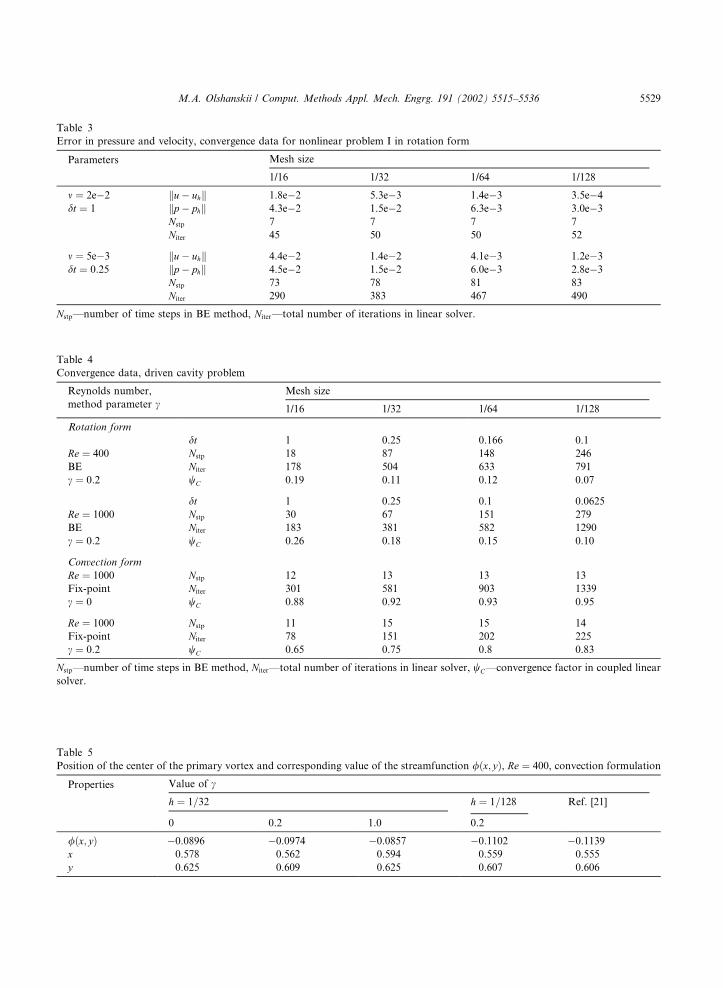
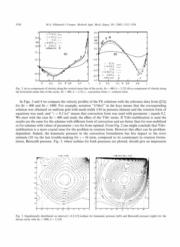
In Figs. 2 and 4 we compare the velocity profiles of the FE solutions with the reference data from ([21])
for Re ¼ 400 and Re ¼ 1000. For example, notation ‘‘1/16(r)’’ in the keys means that the correspondingsolution was obtained on uniform grid with mesh-width 1/16 in pressure element and the rotation form of
equations was used, and ‘‘c ¼ 0:2 (c)’’ means that convection form was used with parameter c equals 0.2.We start with the case Re ¼ 400 and study the effect of the rdiv terms. If rdiv-stabilization is used theresults are the same for the schemes with different form of convection and are better then for non-stabilized
or for schemes with values of parameter c too far from optimal. From Fig. 2 one might conclude that rdiv-stabilization is a more crucial issue for the problem in rotation form. However this effect can be problem-
dependent: Indeed, the kinematic pressure in the convection formulation has less impact to the error
estimate (10 via the last trouble-making for c ¼ 0) term, compared to its counterpart in rotation formu-lation, Bernoulli pressure. Fig. 3, where isolines for both pressures are plotted, should give an impression
Fig. 2. (a) ux-component of velocity along the vertical center line of the cavity, Re ¼ 400, h ¼ 1=32; (b) uy-component of velocity alongthe horizontal center line of the cavity, Re ¼ 400, h ¼ 1=32; c––convection form, r––rotation form.
Fig. 3. Equidistantly distributed on interval [�0:2; 0:3] isolines for kinematic pressure (left) and Bernoulli pressure (right) for thedriven cavity with Re ¼ 1000, h ¼ 1=128.
that H 1 norm of the Bernoulli pressure is large than the same norm of the kinematic pressure for thisparticular problem. We can not claim that this is the case for an arbitrary flow, e.g. for analytical example I
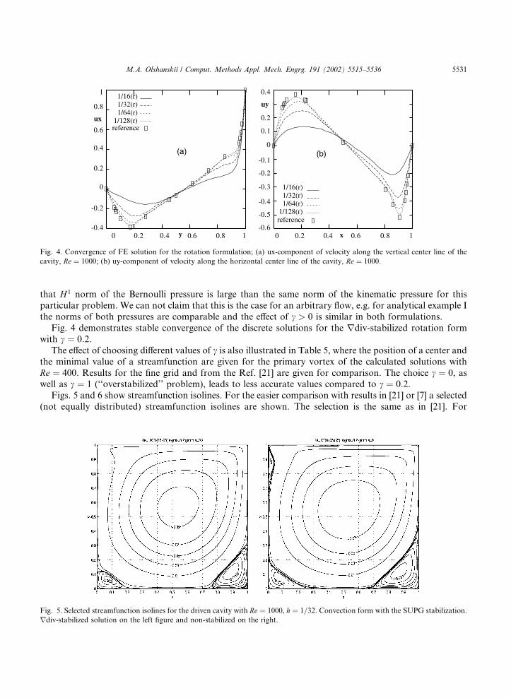
the norms of both pressures are comparable and the effect of c > 0 is similar in both formulations.Fig. 4 demonstrates stable convergence of the discrete solutions for the rdiv-stabilized rotation form
with c ¼ 0:2.The effect of choosing different values of c is also illustrated in Table 5, where the position of a center and
the minimal value of a streamfunction are given for the primary vortex of the calculated solutions with
Re ¼ 400. Results for the fine grid and from the Ref. [21] are given for comparison. The choice c ¼ 0, aswell as c ¼ 1 (‘‘overstabilized’’ problem), leads to less accurate values compared to c ¼ 0:2.Figs. 5 and 6 show streamfunction isolines. For the easier comparison with results in [21] or [7] a selected
(not equally distributed) streamfunction isolines are shown. The selection is the same as in [21]. For
reference1/128(r)
1/64(r)1/32(r)1/16(r)
10.80.6y
(a)
0.40.20
1
0.8
0.6
ux
0.4
0.2
0
-0.2
-0.4reference1/128(r)
1/64(r)1/32(r)1/16(r)
10.80.6x
(b)
0.40.20
0.4
uy
0.2
0.1
0
-0.1
-0.2
-0.3
-0.4
-0.5
-0.6
Fig. 4. Convergence of FE solution for the rotation formulation; (a) ux-component of velocity along the vertical center line of the
cavity, Re ¼ 1000; (b) uy-component of velocity along the horizontal center line of the cavity, Re ¼ 1000.
Fig. 5. Selected streamfunction isolines for the driven cavity with Re ¼ 1000, h ¼ 1=32. Convection form with the SUPG stabilization.rdiv-stabilized solution on the left figure and non-stabilized on the right.
Re ¼ 1000, comparing SUPG stabilized scheme with the usual Galerkin scheme for the convectionformulation, we found that although the SUPG-stabilized solution is a bit more diffusive (less accurate)
than non-stabilized one, the convergence of nonlinear iterations for the stabilized problem is considerablybetter (see also [44]). Moreover, to handle linearized equations in convection form the SUPG stabilization
was also essential to ensure convergence of BiCGstab iterations for ReP 1000:A proper value of c remains to be important. Fig. 5 shows that a solution of the rdiv-stabilized scheme
is more accurate for h ¼ 1=64: On the right figure we see non-physical behaviour of the solution in theupper-left corner of the cavity, also the main vortex is approximated less accurately. For smaller h thedifference becomes less visible, since both stabilized and non-stabilized schemes converge as h ! 0.Moreover the choice of c > 0 reduces the total number of linear iterations (and hence the CPU time)dramatically (see Table 4), although a convergence in the internal multigrid method for the convection–diffusion problem becomes worse. The latter does not alter the total CPU time, since we perform a fixed
number of multigrid cycles applying AA�1 in (25).
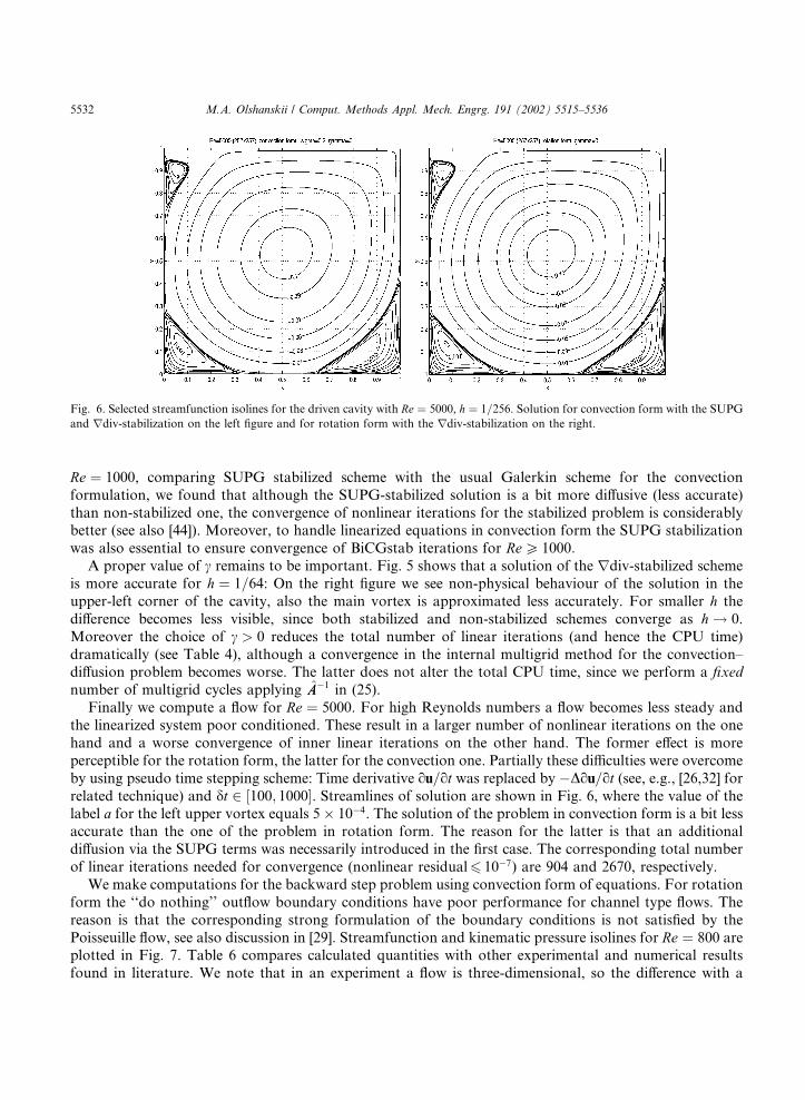
Finally we compute a flow for Re ¼ 5000. For high Reynolds numbers a flow becomes less steady andthe linearized system poor conditioned. These result in a larger number of nonlinear iterations on the one
hand and a worse convergence of inner linear iterations on the other hand. The former effect is more
perceptible for the rotation form, the latter for the convection one. Partially these difficulties were overcome
by using pseudo time stepping scheme: Time derivative ou=ot was replaced by �Dou=ot (see, e.g., [26,32] forrelated technique) and dt 2 ½100; 1000�. Streamlines of solution are shown in Fig. 6, where the value of thelabel a for the left upper vortex equals 5� 10�4. The solution of the problem in convection form is a bit lessaccurate than the one of the problem in rotation form. The reason for the latter is that an additional
diffusion via the SUPG terms was necessarily introduced in the first case. The corresponding total number
of linear iterations needed for convergence (nonlinear residual6 10�7) are 904 and 2670, respectively.
We make computations for the backward step problem using convection form of equations. For rotation
form the ‘‘do nothing’’ outflow boundary conditions have poor performance for channel type flows. The
reason is that the corresponding strong formulation of the boundary conditions is not satisfied by the
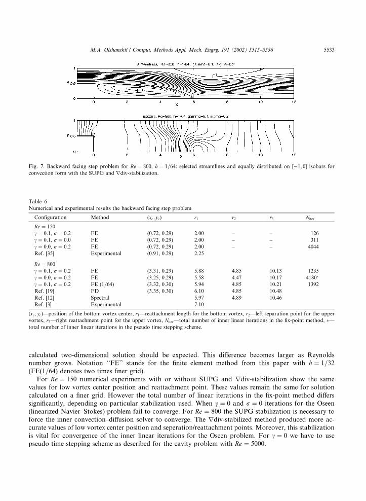
Poisseuille flow, see also discussion in [29]. Streamfunction and kinematic pressure isolines for Re ¼ 800 areplotted in Fig. 7. Table 6 compares calculated quantities with other experimental and numerical results
found in literature. We note that in an experiment a flow is three-dimensional, so the difference with a
Fig. 6. Selected streamfunction isolines for the driven cavity with Re ¼ 5000, h ¼ 1=256. Solution for convection form with the SUPGand rdiv-stabilization on the left figure and for rotation form with the rdiv-stabilization on the right.
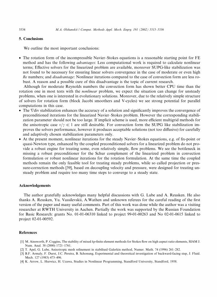
calculated two-dimensional solution should be expected. This difference becomes larger as Reynoldsnumber grows. Notation ‘‘FE’’ stands for the finite element method from this paper with h ¼ 1=32(FE(1=64) denotes two times finer grid).For Re ¼ 150 numerical experiments with or without SUPG and rdiv-stabilization show the same
values for low vortex center position and reattachment point. These values remain the same for solution
calculated on a finer grid. However the total number of linear iterations in the fix-point method differs
significantly, depending on particular stabilization used. When c ¼ 0 and r ¼ 0 iterations for the Oseen(linearized Navier–Stokes) problem fail to converge. For Re ¼ 800 the SUPG stabilization is necessary toforce the inner convection–diffusion solver to converge. The rdiv-stabilized method produced more ac-curate values of low vortex center position and seperation/reattachment points. Moreover, this stabilization
is vital for convergence of the inner linear iterations for the Oseen problem. For c ¼ 0 we have to usepseudo time stepping scheme as described for the cavity problem with Re ¼ 5000.
Fig. 7. Backward facing step problem for Re ¼ 800, h ¼ 1=64: selected streamlines and equally distributed on [�1; 0] isobars forconvection form with the SUPG and rdiv-stabilization.
Table 6
Numerical and experimental results the backward facing step problem
Configuration Method (xc; yc) r1 r2 r3 Niter
Re ¼ 150c ¼ 0:1, r ¼ 0:2 FE (0.72, 0.29) 2.00 – – 126
c ¼ 0:1, r ¼ 0:0 FE (0.72, 0.29) 2.00 – – 311
c ¼ 0:0, r ¼ 0:2 FE (0.72, 0.29) 2.00 – – 4044
Ref. [35] Experimental (0.91, 0.29) 2.25
Re ¼ 800c ¼ 0:1, r ¼ 0:2 FE (3.31, 0.29) 5.88 4.85 10.13 1235
c ¼ 0:0, r ¼ 0:2 FE (3.25, 0.29) 5.58 4.47 10.17 4180�
c ¼ 0:1, r ¼ 0:2 FE (1=64) (3.32, 0.30) 5.94 4.85 10.21 1392
Ref. [19] FD (3.35, 0.30) 6.10 4.85 10.48
Ref. [12] Spectral 5.97 4.89 10.46
Ref. [3] Experimental 7.10
(xc; yc)––position of the bottom vortex center, r1––reattachment length for the bottom vortex, r2––left separation point for the uppervortex, r3––right reattachment point for the upper vortex, Niter––total number of inner linear iterations in the fix-point method, �––total number of inner linear iterations in the pseudo time stepping scheme.
• The rotation form of the incompressible Navier–Stokes equations is a reasonable starting point for FEmethod and has the following advantages: Less computational work is required to calculate nonlinear
terms; Effective solvers for the linearized problem are available, moreover SUPG-like stabilization was
not found to be necessary for ensuring linear solvers convergence in the case of moderate or even highRe numbers; and disadvantage: Nonlinear iterations compared to the case of convection form are less ro-
bust. A reason and a possible cure of this disadvantage is the topic of current research.
Although for moderate Reynolds numbers the convection form has shown better CPU time than the
rotation one in most tests with the nonlinear problem, we expect the situation can change for unsteady
problems, when one is interested in evolutionary solutions. Moreover, due to the relatively simple structure
of solvers for rotation form (block Jacobi smoothers and V-cycles) we see strong potential for parallel
computations in this case.
• The rdiv stabilization enhances the accuracy of a solution and significantly improves the convergence ofpreconditioned iterations for the linearized Navier–Stokes problem. However the corresponding stabili-
zation parameter should not be too large. If implicit scheme is used, more efficient multigrid methods for
the anisotropic case m=c � 1 are still desirable. For convection form the SUPG like stabilization im-proves the solvers performance, however it produces acceptable solutions (not too diffusive) for carefully
and adaptively chosen stabilization parameters only.
• At the present moment, nonlinear iterations for the steady Navier–Stokes equations, e.g. of fix-point orquasi-Newton type, enhanced by the coupled preconditioned solvers for a linearized problem do not pro-
vide a robust engine for treating some, even relatively simple, flow problems. We see the bottleneck inmissing a robust preconditioner for the Schur complement of the linearized problem in convection
formulation or robust nonlinear iterations for the rotation formulation. At the same time the coupled
methods remain the only feasible tool for treating steady problems, while so called projection or pres-
sure-correction methods [39], based on decoupling velocity and pressure, were designed for treating un-
steady problem and require too many time steps to converge to a steady state.
Acknowledgements
The author gratefully acknowledges many helpful discussions with G. Lube and A. Reusken. He also
thanks A. Reusken, Yu. Vassilevskii, A.Wathen and unknown referees for the careful reading of the first
version of the paper and many useful comments. Part of this work was done while the author was a visiting
researcher at RWTH University in Aachen. Partially the work was supported by the Russian Foundation
for Basic Research: grants No. 01-01-06310 linked to project 99-01-00263 and No 02-01-0615 linked to
project 02-01-00592.
References
[1] M. Ainsworth, P. Coggins, The stability of mixed hp-finite element methods for Stokes flow on high aspect ratio elements, SIAM J.Num. Anal. 38 (2000) 1721–1761.
[2] T. Apel, G. Lube, Anisotropic mesh refinement in stabilised Galerkin method, Numer. Math. 74 (1996) 261–282.
[3] B.F. Armaly, F. Durst, J.C. Pereira, B. Schonung, Experimental and theoretical investigation of backward-facing step, J. Fluid.
Mech. 127 (1983) 473–496.
[4] K. Arrow, L. Hurwicz, H. Uzawa, Studies in Nonlinear Programming, Standford University, Standford, 1958.
[29] J.G. Heywood, R. Rannacher, S. Turek, Artificial boundaries and flux and pressure conditions for the incompressible Navier–
Stokes equations, Int. J. Numer. Meth. Fluids 22 (1996) 325–352.
[30] A. Klawonn, G. Starke, Block triangular preconditioners for nonsymmetric saddle point problem, Numer. Math. 81 (1999) 577–
594.
[31] D. Kay, D. Loghin, A Green�s function preconditioner for the steady state Navier–Stokes equations, Oxford UniversityComputing Lab., Report 99/06, 1999.
[32] G.M. Kobelkov, On numerical methods of solving the Navier–Stokes equations in ‘‘velocity-pressure’’ variables, in: G.I. Marchuk
(Ed.), Numerical Methods and Applications, CRC, New York, 1994, pp. 85–115.
[33] G. Lube, Stabilized Galerkin finite element methods for convection dominated and incompressible flow problems, Numer. Anal.
Math. Model. (Banach center publications) 29 (1994) 85–104.
[34] G. Lube, M.A. Olshanskii, Stable finite element calculation of incompressible flow using the rotational form of convection, IMA J.


![A discontinuous Galerkin reduced basis numerical ...€¦ · theory [9,22,24] that studies the limit of the fine scale Stokes model when the pore size tends to zero. The homogenization](https://static.documents.pub/doc/80x56/60620fa2389c63538a63c623/a-discontinuous-galerkin-reduced-basis-numerical-theory-92224-that-studies.jpg)


