A M -T OBJECTIVE FOR LEARNING TO DISENTANGLE C …

Published as a conference paper at ICLR 2020

A META-TRANSFER OBJECTIVE FOR LEARNING TODISENTANGLE CAUSAL MECHANISMS

Yoshua Bengio1, 2, 5 Tristan Deleu1 Nasim Rahaman4 Nan Rosemary Ke3

Sébastien Lachapelle1 Olexa Bilaniuk1 Anirudh Goyal1 Christopher Pal3, 5

Mila – Montreal, Quebec, Canada

ABSTRACT

We propose to use a meta-learning objective that maximizes the speed of transferon a modified distribution to learn how to modularize acquired knowledge anddiscover causal dependencies. In particular, we focus on how to factor a jointdistribution into appropriate conditionals, consistent with the causal directions. Toreplace the assumption that the test cases are of the same distribution as the trainingexamples, this method exploits the assumption that the changes in distributionsare localized (e.g. to one of the marginals, for example due to an interventionon a cause). We prove that under this assumption of localized changes in causalmechanisms, the correct causal graph will tend to have only a few of its param-eters with non-zero gradient, i.e. that need to be adapted (those of the modifiedvariables). We argue and observe experimentally that this leads to faster adaptation,and use this property to define a meta-learning surrogate score which, in additionto a continuous parametrization of graphs, would favour correct causal graphs,making it possible to discover causal structure by gradient-based methods. Finally,motivated by the AI agent point of view (e.g. of a robot discovering its environ-ment autonomously), we consider how the same objective can discover the causalvariables themselves, as a transformation of observed low-level variables with nocausal meaning. Experiments in the two-variable case validate the proposed ideasand theoretical results.

1 INTRODUCTION

The data used to train our models is often assumed to be independent and identically distributed (iid.),according to some unknown distribution. Likewise, the performance of a machine learning model istypically evaluated using test samples from the same distribution, assumed to be representative ofthe learned system’s usage. While these assumptions are well analyzed from a statistical point ofview, they are rarely satisfied in many real-world applications. For example, an accident on a majorhighway could completely perturb the trajectories of cars, and a driving policy trained in a static waymight not be robust to such changes. Ideally, we would like our models to generalize well and adaptquickly to out-of-distribution data.

However, this comes at a price – in order to successfully transfer to a novel distribution, onemight need additional information about these distributions. In this paper, we are not consideringassumptions on the data distribution itself, but rather on how it changes (e.g., when going from atraining distribution to a transfer distribution, possibly resulting from some agent’s actions). We focuson the assumption that the changes are sparse when the knowledge is represented in an appropriatelymodularized way, with only one or a few of the modules having changed. This is especially relevantwhen the distributional change is due to actions by one or more agents, because agents interveneat a particular place and time, and this is reflected in the form of the interventions discussed inthe causality literature (Pearl, 2009; Peters et al., 2016), where a single causal variable is clampedto a particular value or a random variable. In general, it is difficult for agents to influence manyunderlying causal variables at a time, and although this paper is not about agent learning as such,this is a property of the world that we propose to exploit here, to help discovering these variables

1 Université de Montréal, 2 CIFAR Senior Fellow, 3 École Polytechnique Montréal, 4 Max-Planck Institutefor Intelligent Systems, Tübingen, 5 Canada CIFAR AI Chair

1


and how they are causally related to each other. In this context, the causal graph is a powerful toolbecause it tells us how perturbations in the distribution of intervened variables will propagate to allother variables and affect their distributions.

As expected, it is often the case that the causal structure is not known in advance. The problem ofcausal discovery then entails obtaining the causal graph, a feat which is in general achievable onlywith strong assumptions. One such assumption is that a learner that has learned to capture the correctstructure of the true underlying data-generating process should still generalize to the case where thestructure has been perturbed in a certain, restrictive way. This can be illustrated by considering theexample of temperature and altitude from Peters et al. (2017): a learner that has learned to capture themechanisms of atmospheric physics by learning that it makes more sense to predict temperature fromthe altitude (rather than vice versa) given training data from (say) Switzerland, will still remain validwhen tested on out-of-distribution data from a less mountainous country like (say) the Netherlands. Ithas therefore been suggested that the out-of-distribution robustness of predictive models can be usedto guide the inference of the true causal structure (Peters et al., 2016; 2017).

How can we exploit the assumption of localized change? As we explain theoretically and verifyexperimentally here, if we have the right knowledge representation, then we should get fast adaptationto the transfer distribution when starting from a model that is well trained on the training distribution.This arises because of our assumption that the ground truth data generative process is obtainedas the composition of independent mechanisms, and that very few ground truth mechanisms andparameters need to change when going from the training distribution to the transfer distribution. Amodel capturing a corresponding factorization of knowledge would thus require just a few updates, afew examples, for this adaptation to the transfer distribution. As shown below, the expected gradienton the unchanged parameters would be near 0 (if the model was already well trained on the trainingdistribution), so the effective search space during adaptation to the transfer distribution would begreatly reduced, which tends to produce faster adaptation, as found experimentally. Thus, basedon the assumption of small change in the right knowledge representation space, we can define ameta-learning objective that measures the speed of online adaptation in order to optimize the way inwhich knowledge should be represented, factorized and structured. This is the core idea presented inthis paper.

Returning to the example of temperature and altitude: when presented with out-of-distribution datafrom the Netherlands, we expect the correct model to adapt faster given a few transfer samples ofactual weather data collected in the Netherlands. Analogous to the case of robustness, the adaptationspeed can then be used to guide the inference of the true causal structure of the problem at hand,possibly along with other sources of signal about causal structure.

Contributions. We first verify on synthetic data that the model that correctly captures the underlyingcausal structure adapts faster when presented with data sampled after a performing certain interven-tions on the true two-variable causal graph (which is unknown to the learner). This suggests that theadaptation speed can indeed function as a score to assess how well the learner fits the underlyingcausal graph. We then use a smooth parameterization of the considered causal graph to directlyoptimize this score in an end-to-end gradient-based manner. Finally, we show in a simple setting thatthe score can be exploited to disentangle the correct causal variables given an unknown mixture ofthe said variables.

2 WHICH IS CAUSE AND WHICH IS EFFECT?As an illustrative example of the proposed ideas, let us consider two discrete random variables Aand B, each taking N possible values. We assume that A and B are correlated, without any hiddenconfounder. Our goal is to determine whether the underlying causal graph is A→ B (A causes B),or B → A. Note that this underlying causal graph cannot be identified from observational data froma single (training) distribution p only, since both graphs are Markov equivalent for p (Verma & Pearl,1991); see Appendix A. In order to disambiguate between these two hypotheses, we will use samplesfrom some transfer distribution p̃ in addition to our original samples from the training distribution p.

2.1 THE ADVANTAGE OF THE CORRECT CAUSAL MODEL

Without loss of generality, we can fix the true causal graph to be A → B, which is unknown tothe learner. Moreover, to make the case stronger, we will consider a setting called covariate shift(Rojas-Carulla et al., 2018; Quionero-Candela et al., 2009), where we assume that the change (again,

2


whose nature is unknown to the learner) between the training and transfer distributions occurs afteran intervention on the cause A. In other words, the marginal of A changes, while the conditionalp(B | A) does not, i.e. p(B | A) = p̃(B | A). Changes on the cause will be most informative, sincethey will have direct effects on B. This is sufficient to fully identify the causal graph (Hauser &Bühlmann, 2012).

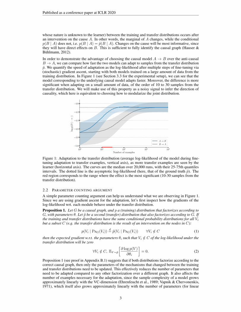
In order to demonstrate the advantage of choosing the causal model A → B over the anti-causalB → A, we can compare how fast the two models can adapt to samples from the transfer distributionp̃. We quantify the speed of adaptation as the log-likelihood after multiple steps of fine-tuning via(stochastic) gradient ascent, starting with both models trained on a large amount of data from thetraining distribution. In Figure 1 (see Section 3.3 for the experimental setup), we can see that themodel corresponding to the underlying causal model adapts faster. Moreover, the difference is moresignificant when adapting on a small amount of data, of the order of 10 to 30 samples from thetransfer distribution. We will make use of this property as a noisy signal to infer the direction ofcausality, which here is equivalent to choosing how to modularize the joint distribution.

100 101 102 103 104

Number of examples

−5.0

−4.8

−4.6

−4.4

−4.2

−4.0

logp(D|·→·)

A→ B

B → A

Figure 1: Adaptation to the transfer distribution (average log-likelihood of the model during fine-tuning adaptation to transfer examples, vertical axis), as more transfer examples are seen by thelearner (horizontal axis). The curves are the median over 20,000 runs, with their 25-75th quantilesintervals. The dotted line is the asymptotic log-likelihood (here, that of the ground truth p̃). Thered region corresponds to the range where the effect is the most significant (10-30 samples from thetransfer distribution).

2.2 PARAMETER COUNTING ARGUMENT

A simple parameter counting argument can help us understand what we are observing in Figure 1.Since we are using gradient ascent for the adaptation, let’s first inspect how the gradients of thelog-likelihood wrt. each module behave under the transfer distribution.Proposition 1. Let G be a causal graph, and p a (training) distribution that factorizes according toG, with parameters θ. Let p̃ be a second (transfer) distribution that also factorizes according to G. Ifthe training and transfer distributions have the same conditional probability distributions for all Vibut a subset C (e.g. the transfer distribution is the result of an intervention on the nodes in C):

p(Vi | PaG(Vi))d= p̃(Vi | PaG(Vi)) ∀Vi /∈ C (1)

then the expected gradient w.r.t. the parameters θi such that Vi /∈ C of the log-likelihood under thetransfer distribution will be zero

∀Vi /∈ C, EV∼p̃[∂ log p(V )

∂θi

]= 0. (2)

Proposition 1 (see proof in Appendix B.1) suggests that if both distributions factorize according to thecorrect causal graph, then only the parameters of the mechanisms that changed between the trainingand transfer distributions need to be updated. This effectively reduces the number of parameters thatneed to be adapted compared to any other factorization over a different graph. It also affects thenumber of examples necessary for the adaptation, since the sample complexity of a model growsapproximately linearly with the VC-dimension (Ehrenfeucht et al., 1989; Vapnik & Chervonenkis,1971), which itself also grows approximately linearly with the number of parameters (for linear

3


models and neural networks; Shalev-Shwartz & Ben-David, 2014). Therefore we argue that theperformance on the transfer distribution (in terms of log-likelihood) will tend to improve faster if itfactorizes according to the correct causal graph, an assertion which may not be true for every graphbut that we can test by simulations.

Recall that in our example on two discrete random variables (each taking say N values), we assumedthat the underlying causal model isA→ B, and the transfer distribution is the result of an interventionon the cause A. If the model we learn on the training distribution factorizes according to the correctgraph, then only N − 1 free parameters should be updated to adapt to the shifted distribution,accounting for the change in the marginal distribution p̃(A), since the conditional p̃(B | A) = p(B |A) stays invariant. On the other hand, if the model factorizes according to the anti-causal graphB → A, then the parameters for both the marginal p̃(B) and the conditional p̃(A | B) must beadapted. Assuming there is a linear relationship between sample complexity and the number of freeparameters, the sample complexity would be O(N2) for the anti-causal graph, compared to onlyO(N) for the true underlying causal graph A→ B.

3 THE META-TRANSFER OBJECTIVE

Since the speed of adaptation to some transfer distribution is closely related to the right modularizationof knowledge, we propose to use it as a noisy signal to iteratively improve inference of the causalstructure from data. Moreover, we saw in Figure 1 that the gap between correct and incorrect modelsis largest with a small amount of transfer data. In order to compare how fast some models adapt to achange in distribution, we can quantify the speed of adaptation based on their accumulated onlineperformance after fine-tuning with gradient ascent on few examples from the transfer distribution.More precisely, given a small “intervention” datasetDint = {xt}Tt=1 from p̃, we can define the onlinelikelihood as

LG(Dint) =

T∏

t=1

p(xt ; θ(t)G , G)

θ(1)G = θ̂ML

G (Dobs)θ

(t+1)G = θ

(t)G + α∇θ log p(xt ; θ

(t)G , G),

(3)

where θ(t)G aggregates all the modules’ parameters in G after t steps of fine-tuning with gradient

ascent, with learning rate α, starting from the maximum-likelihood estimate θ̂MLG (Dobs) on a large

amount of data Dobs from the training distribution p. Note that, in addition to its contribution tothe update of the parameters, each data point xt is also used to evaluate the performance of ourmodel so far; this is called a prequential analysis (Dawid, 1984), also corresponding to sequentialcross-validation (Gingras et al., 1999). From a structure learning perspective, the online likelihood(or, equivalently, its logarithm) can be interpreted as a score we would like to maximize, in order torecover the correct causal graph.

3.1 CONNECTION TO THE BAYESIAN SCORE

We can draw an interesting connection between the online log-likelihood, and a widely used score instructure learning called the Bayesian score (Heckerman et al., 1995; Geiger & Heckerman, 1994).The idea behind this score is to treat the problem of learning the structure from a fully Bayesianperspective. If we define a prior over graphs p(G) and a prior p(θG | G) over the parameters of eachgraph G, the Bayesian score is defined as scoreB(G ; Dint) = log p(Dint | G) + log p(G), wherep(Dint | G) is the marginal likelihood

p(Dint | G) =

T∏

t=1

p(xt | x1, . . . ,xt−1, G) =

T∏

t=1

[ ∫

ΘG

p(xt | θG, G)p(θG | x1:t−1, G) dθG

].

(4)In the online likelihood, the adapted parameters θ(t)

G act as a summary of past data x1:t−1. Eq. (3)can be seen as an approximation of the marginal likelihood in Eq. (4), where the posteriors overthe parameters p(θG | x1:t−1, G) is approximated by the point estimate θ(t)

G . Therefore, the onlinelog-likelihood provides a simple way to approximate the Bayesian score, which is often intractable.

3.2 A SMOOTH PARAMETRIZATION OF THE CAUSAL STRUCTURE

Due to the super-exponential number of possible Directed Acyclic Graphs (DAGs) over n nodes,the problem of searching for a causal structure that maximizes some score is, in general, NP-hard

4


(Chickering, 2002a). However, we can parametrize our belief about causal graphs by keeping trackof the probability for each directed edge to be present. This provides a smooth parametrization ofgraphs, which hinges on gradually changing our belief in individual binary decisions associated witheach edge of the causal graph. This allows us to define a fully differentiable meta-learning objective,with all the beliefs being updated at the same time by gradient descent.

In this section, we study the simplest version of this idea, applied to our example on two randomvariables from Section 2. Recall that here, we only have two hypotheses to choose from: eitherA→ B or B → A. We represent our belief of having an edge connecting A to B with a structuralparameter γ such that p(A→ B) = σ(γ), where σ(γ) = 1/(1 + exp(−γ)) is the sigmoid function.We propose, as a meta-transfer objective, the negative log-likelihoodR (a form of regret) over themixture of these two models, where the mixture parameter is given by σ(γ):

R(Dint) = − log [σ(γ)LA→B(Dint) + (1− σ(γ))LB→A(Dint)] (5)This meta-learning mixture combines the online adaptation likelihoods of each model over onemeta-example or episode (specified by a Dint ∼ p̃), rather than considering and linearly mixing theper-example likelihoods as in ordinary mixtures.

In the experiments below, after each episode involving T examplesDint from the transfer distributionp̃, we update γ by doing one step of gradient descent, to reduce the regretR. Therefore, in order toupdate our belief about the edge A→ B, the quantity of interest is the gradient of the objectiveRwith respect to the structural parameter, ∂R/∂γ. This gradient is pushing σ(γ) towards the posteriorprobability that the correct model is A→ B, given the evidence from the transfer data:Proposition 2. The gradient of the negative log-likelihood of the transfer data Dint in Equation (5)wrt. the structural parameter γ is given by

∂R∂γ

= p(A→ B)− p(A→ B | Dint), (6)

where p(A→ B | Dint) is the posterior probability of the hypothesis A→ B (when the alternativeis B → A). Furthermore, this can be equivalently written as

∂R∂γ

= σ(γ)− σ(γ + ∆), (7)

where ∆ = logLA→B(Dint)− logLB→A(Dint) is the difference between the online log-likelihoodsof the two hypotheses on the transfer data Dint.The proof is given in Appendix B.2. Note how the posterior probability is basically measuring whichhypothesis is better explaining the transfer data Dint overall, along the adaptation trajectory. Thisposterior depends on the difference in online log-likelihoods ∆, showing the close relation betweenminimizing the regretR and maximizing the online log-likelihood score. The sign and magnitudeof ∆ have a direct effect on the convergence of the meta-transfer objective. We can show that themeta-transfer objective is guaranteed to converge to one of the two hypotheses.Proposition 3. With stochastic gradient descent (and an appropriately decreasing learning rate)on EDint

[R(Dint)], where the gradient steps are given by Proposition 2, the structural parameterconverges towards

σ(γ)→ 1 if EDint [LA→B(Dint)] > EDint [LB→A(Dint)]or σ(γ)→ 0 otherwise

(8)

This proposition (proved in Appendix B.3) shows that optimizing γ is equivalent to picking thehypothesis that has the smallest regret (or fastest convergence), measured as the accumulated log-likelihood of the transfer dataset Dint during adaptation. The distribution over datasets Dint issimilar to a distribution over tasks in meta-learning. This analogy with meta-learning also appearsin our gradient-based adaptation procedure, which is linked to existing methods like the first-orderapproximation of MAML (Finn et al., 2017), and its related algorithms (Grant et al., 2018; Kim et al.,2018; Finn et al., 2018). The pseudo-code for the proposed algorithm is given in Algorithm 1.

This smooth parametrization of the causal graph, along with the definition of the meta-transferobjective in Equation (5), can be extended to graphs with more than 2 variables. This generalformulation builds on the bivariate case, where decisions are binary for each individual edge of thegraph. See Appendix E for details and a generalization of Proposition 2; the structure of Algorithm 1remains unchanged. Experimentally, this generalization of the meta-transfer objective proved to beeffective on larger graphs (Ke et al., 2019), in work following the initial release of this paper.

5


Algorithm 1 Meta-learning algorithm for learning the structural parameterRequire: Two graph candidates G = A→ B and G = B → ARequire: A training distribution p that factorizes over the correct causal graph

1: Set the initial structural parameter γ = 0 . equal belief for both hypotheses2: Sample a large dataset Dobs from the training distribution p3: Pretrain the parameters of both models with maximum likelihood on Dobs4: for each episode do5: Draw a transfer distribution p̃ (via an intervention)6: Sample a (small) transfer dataset Dint = {xt}Tt=1 from p̃7: for t = 1, . . . , T do8: Accumulate the online log-likelihood for both models LA→B and LB→A as they adapt9: Do one step of gradient ascent for both models: θ(t+1)

G = θ(t)G + α∇θ log p(xt ; θ

(t)G , G)

10: Compute the regretR(Dint)11: Compute the gradient of the regret wrt. γ (see Proposition 2)12: Do one step of gradient descent on the regret w.r.t. γ13: Reset the models’ parameters to the maximum likelihood estimate on Dobs

3.3 EXPERIMENTAL RESULTS

To illustrate the convergence result from Proposition 3, we experiment with learning the structuralparameter γ in a bivariate model. Following the setting presented in Section 2.1, we assume in allour experiments that A and B are two correlated random variables, and the underlying causal model(unknown to the algorithm) is fixed to A→ B. Recall that both variables are observed, and there isno hidden confounding factor. Since the correct causal model is A → B, the structural parametershould converge correctly, with σ(γ)→ 1. The details of the experimental setups, as well as detailsabout the models, can be found in Appendix C.

We first experiment with the case where both A and B are discrete random variables, taking Npossible values. In this setting, we explored how two different parametrizations of the conditionalprobability distributions (CPDs) might influence the convergence of the structural parameter. In thefirst experiment, we parametrized the CPDs as multinomial logistic CPDs (Koller & Friedman, 2009),maintaining a tabular representation of the conditional probabilities. For example, the conditionaldistribution p(B | A) is represented as

p(B = j | A = i ; θ) =exp(θij)∑k exp(θik)

, (9)

where the parameter θ is an N ×N matrix. We used a similar representation for the other marginaland conditional distributions p(A), p(B) and p(A | B). In a second experiment, we used structuredCPDs, parametrized with multi-layer perceptrons (MLPs) with a softmax nonlinearity at the outputlayer. The advantage over a tabular representation is the ability to share parameters for similarcontexts, and reduces the overall number of parameters required for each module. This would becrucial if either the number of categories N , or the number of variables, increased significantly.

0 100 200 300 400 500Number of episodes

0.0

0.2

0.4

0.6

0.8

1.0

σ(γ

)

N = 10

N = 100

A B

A B


0.0

0.2

0.4

0.6

0.8

1.0

σ(γ

)

N = 10

N = 100

A B

A B

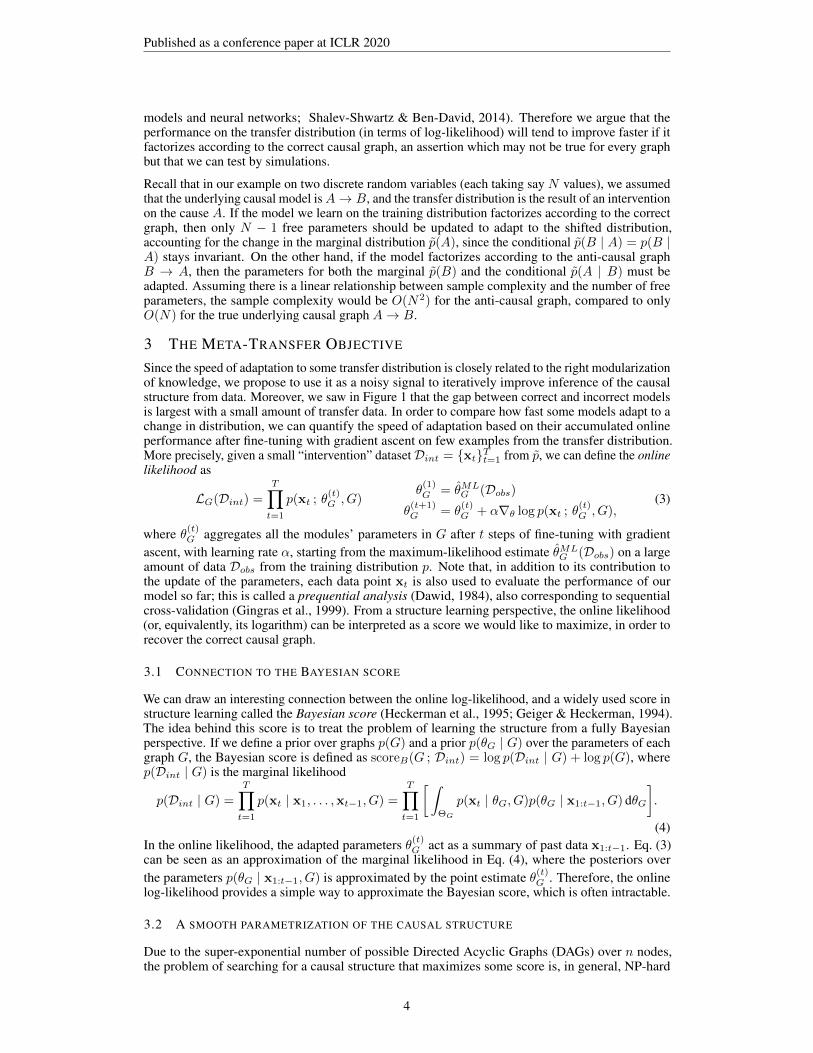
Figure 2: Evolution of the belief that A→ B is the correct causal model, as the number of episodesincreases, starting with an equal belief for both hypotheses. (Left) multinomial logistic CPDs, (right)MLP parametrization.

6


In Figure 2, we show the evolution of σ(γ), which is the model’s belief of A→ B being the correctcausal model, as the number of episodes increases, for different values of N . As expected, the struc-tural parameter converges correctly to σ(γ)→ 1, within a few hundreds episodes. This observationis consistent in both experiments, regardless of the parametrization of the CPDs. Interestingly, thestructural parameter tends to converge faster with a larger value of N and a tabular representation,illustrating the effect of the parameter counting argument described in Section 2.2, which is strongeras N increases. Precisely when generalization is more difficult (too many parameters and too fewexamples), we get a stronger signal about the better modularization.

We also experimented with A and B being continuous random variables, where they follow eithermultimodal distributions, or they are linear-Gaussian. Similar to Figure 2, we found that the structuralparameter σ(γ) consistently converges to the correct causal model as well. See Appendix C.3 andAppendix C.4 for details about these experiments.

4 REPRESENTATION LEARNING

So far, we have assumed that all the variables in the causal graph are fully observed. However, in manyrealistic scenarios for learning agents, the learner might only have access to low-level observations(e.g. sensory-level data, like pixels or acoustic samples), which are very unlikely to be individuallymeaningful as causal variables. In that case, our assumption that the changes in distributions arelocalized might not hold at this level of observed data. To tackle this, we propose to follow the deeplearning objective of disentangling the underlying causal variables (Bengio et al., 2013), and learn arepresentation in which the variables can be meaningfully cause or effect of each other. Our approachis to jointly learn this representation, as well as the causal graph over the latent variables.

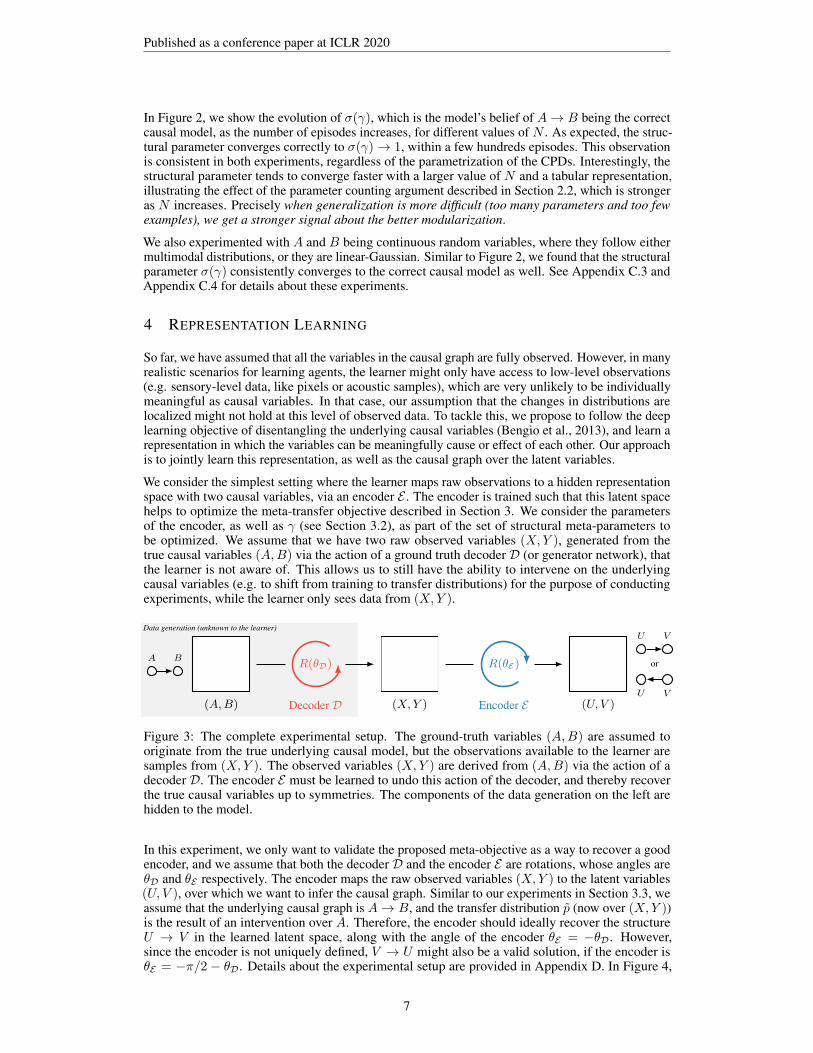
We consider the simplest setting where the learner maps raw observations to a hidden representationspace with two causal variables, via an encoder E . The encoder is trained such that this latent spacehelps to optimize the meta-transfer objective described in Section 3. We consider the parametersof the encoder, as well as γ (see Section 3.2), as part of the set of structural meta-parameters tobe optimized. We assume that we have two raw observed variables (X,Y ), generated from thetrue causal variables (A,B) via the action of a ground truth decoder D (or generator network), thatthe learner is not aware of. This allows us to still have the ability to intervene on the underlyingcausal variables (e.g. to shift from training to transfer distributions) for the purpose of conductingexperiments, while the learner only sees data from (X,Y ).

Data generation (unknown to the learner)

R(θD) R(θE)

(A,B) (X,Y ) (U, V )Decoder D Encoder E

A B

U

U

V

V

or

Figure 3: The complete experimental setup. The ground-truth variables (A,B) are assumed tooriginate from the true underlying causal model, but the observations available to the learner aresamples from (X,Y ). The observed variables (X,Y ) are derived from (A,B) via the action of adecoder D. The encoder E must be learned to undo this action of the decoder, and thereby recoverthe true causal variables up to symmetries. The components of the data generation on the left arehidden to the model.

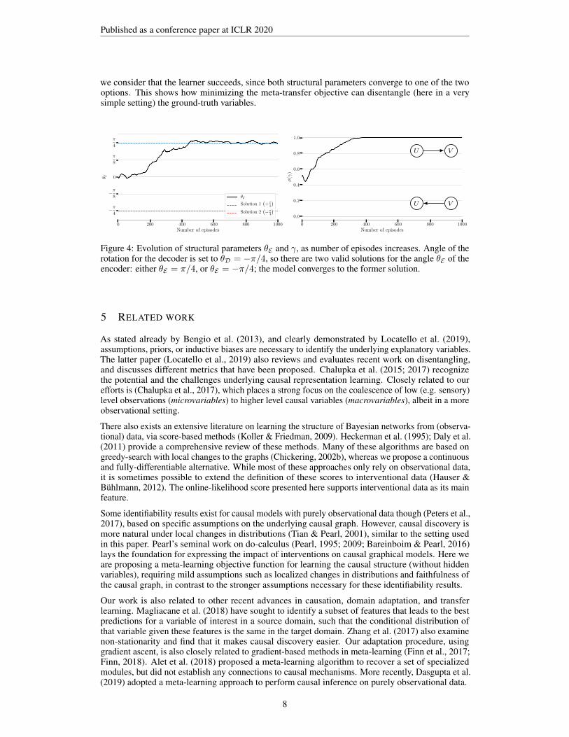
In this experiment, we only want to validate the proposed meta-objective as a way to recover a goodencoder, and we assume that both the decoder D and the encoder E are rotations, whose angles areθD and θE respectively. The encoder maps the raw observed variables (X,Y ) to the latent variables(U, V ), over which we want to infer the causal graph. Similar to our experiments in Section 3.3, weassume that the underlying causal graph is A→ B, and the transfer distribution p̃ (now over (X,Y ))is the result of an intervention over A. Therefore, the encoder should ideally recover the structureU → V in the learned latent space, along with the angle of the encoder θE = −θD. However,since the encoder is not uniquely defined, V → U might also be a valid solution, if the encoder isθE = −π/2 − θD. Details about the experimental setup are provided in Appendix D. In Figure 4,

7


we consider that the learner succeeds, since both structural parameters converge to one of the twooptions. This shows how minimizing the meta-transfer objective can disentangle (here in a verysimple setting) the ground-truth variables.


−π4

−π8

0

π

8

π

4

θ E

θE

Solution 1(+π

4

)

Solution 2(−π

4

)


0.0

0.2

0.4

0.6

0.8

1.0

σ(γ

)

U V

U V

Figure 4: Evolution of structural parameters θE and γ, as number of episodes increases. Angle of therotation for the decoder is set to θD = −π/4, so there are two valid solutions for the angle θE of theencoder: either θE = π/4, or θE = −π/4; the model converges to the former solution.

5 RELATED WORK

As stated already by Bengio et al. (2013), and clearly demonstrated by Locatello et al. (2019),assumptions, priors, or inductive biases are necessary to identify the underlying explanatory variables.The latter paper (Locatello et al., 2019) also reviews and evaluates recent work on disentangling,and discusses different metrics that have been proposed. Chalupka et al. (2015; 2017) recognizethe potential and the challenges underlying causal representation learning. Closely related to ourefforts is (Chalupka et al., 2017), which places a strong focus on the coalescence of low (e.g. sensory)level observations (microvariables) to higher level causal variables (macrovariables), albeit in a moreobservational setting.

There also exists an extensive literature on learning the structure of Bayesian networks from (observa-tional) data, via score-based methods (Koller & Friedman, 2009). Heckerman et al. (1995); Daly et al.(2011) provide a comprehensive review of these methods. Many of these algorithms are based ongreedy-search with local changes to the graphs (Chickering, 2002b), whereas we propose a continuousand fully-differentiable alternative. While most of these approaches only rely on observational data,it is sometimes possible to extend the definition of these scores to interventional data (Hauser &Bühlmann, 2012). The online-likelihood score presented here supports interventional data as its mainfeature.

Some identifiability results exist for causal models with purely observational data though (Peters et al.,2017), based on specific assumptions on the underlying causal graph. However, causal discovery ismore natural under local changes in distributions (Tian & Pearl, 2001), similar to the setting usedin this paper. Pearl’s seminal work on do-calculus (Pearl, 1995; 2009; Bareinboim & Pearl, 2016)lays the foundation for expressing the impact of interventions on causal graphical models. Here weare proposing a meta-learning objective function for learning the causal structure (without hiddenvariables), requiring mild assumptions such as localized changes in distributions and faithfulness ofthe causal graph, in contrast to the stronger assumptions necessary for these identifiability results.

Our work is also related to other recent advances in causation, domain adaptation, and transferlearning. Magliacane et al. (2018) have sought to identify a subset of features that leads to the bestpredictions for a variable of interest in a source domain, such that the conditional distribution ofthat variable given these features is the same in the target domain. Zhang et al. (2017) also examinenon-stationarity and find that it makes causal discovery easier. Our adaptation procedure, usinggradient ascent, is also closely related to gradient-based methods in meta-learning (Finn et al., 2017;Finn, 2018). Alet et al. (2018) proposed a meta-learning algorithm to recover a set of specializedmodules, but did not establish any connections to causal mechanisms. More recently, Dasgupta et al.(2019) adopted a meta-learning approach to perform causal inference on purely observational data.

8


6 DISCUSSION & FUTURE WORK

We have established, in very simple bivariate settings, that the rate at which a learner adapts tosparse changes in the distribution of observed data can be exploited to infer the causal structure, anddisentangle the causal variables. This relies on the assumption that with the correct causal structure,those distributional changes are localized. We have demonstrated these ideas through some theoreticalresults, as well as experimental validation. The source code for the experiments is available here:https://bit.ly/2M6X1al.

This work is only a first step in the direction of causal structure learning based on the speed ofadaptation to modified distributions. On the experimental side, many settings other than those studiedhere should be considered, with different kinds of parametrizations, richer and larger causal graphs(see already Ke et al. (2019), based on a first version of this paper), or different kinds of optimizationprocedures. On the theoretical side, much more needs to be done to formally link the localityof interventions to faster adaptation, to clarify the conditions for this to work. Also, more workneeds to be done in exploring how the proposed ideas can be used to learn good representations inwhich the causal variables are disentangled. Scaling up these ideas would permit their applicationtowards improving the way learning agents deal with non-stationarities, and thus improving samplecomplexity and robustness of these agents.

An extreme view of disentangling is that the explanatory variables should be marginally independent,and many deep generative models (Goodfellow et al., 2016), and Independent Component Analysismodels (Hyvärinen et al., 2001; Hyvärinen et al., 2018), are built on this assumption. However, thekinds of high-level variables that we manipulate with natural language are not marginally independent:they are related to each other through statements that are usually expressed in sentences (e.g. asentence in natural language, or a classical symbolic AI fact or rule), involving only a few concepts ata time. This kind of assumption has been proposed to help discover relevant high-level representationsfrom raw observations, such as the consciousness prior (Bengio, 2017), with the idea that humansfocus at any particular time on just a few concepts that are present to our consciousness. The workpresented here could provide an interesting meta-learning approach to help learn such encodersoutputting causal variables, as well as figure out how the resulting variables are related to each other.In that case, one should distinguish two important assumptions: the first one is that the causal graphis sparse, which a common assumption in structure learning (Schmidt et al., 2007); the second is thatthe changes in distributions are sparse, which is the focus of this work.

REFERENCES

Ferran Alet, Tomás Lozano-Pérez, and Leslie P Kaelbling. Modular meta-learning. arXiv preprintarXiv:1806.10166, 2018.

Elias Bareinboim and Judea Pearl. Causal inference and the data-fusion problem. Proceedings of theNational Academy of Sciences, 2016.

Yoshua Bengio. The Consciousness Prior. arXiv preprint arXiv:1709.08568, 2017.

Yoshua Bengio, Aaron Courville, and Pascal Vincent. Representation Learning: A Review and NewPerspectives. IEEE transactions on pattern analysis and machine intelligence, 2013.

Christopher M Bishop. Mixture Density Networks. Technical report, 1994.

David Blackwell. Conditional Expectation and Unbiased Sequential Estimation. The Annals ofMathematical Statistics, 1947.

Krzysztof Chalupka, Pietro Perona, and Frederick Eberhardt. Visual causal feature learning. Confer-ence on Uncertainty in Artificial Intelligence (UAI) 2015, 2015.

Krzysztof Chalupka, Frederick Eberhardt, and Pietro Perona. Causal feature learning: an overview.Behaviormetrika, 2017.

David Maxwell Chickering. Learning equivalence classes of Bayesian-network structures. Journal ofmachine learning research, 2002a.

9

https://bit.ly/2M6X1al


David Maxwell Chickering. Optimal structure identification with greedy search. Journal of machinelearning research, 2002b.

Rónán Daly, Qiang Shen, and Stuart Aitken. Learning Bayesian networks: approaches and issues.The knowledge engineering review, 2011.

Ishita Dasgupta, Jane Wang, Silvia Chiappa, Jovana Mitrovic, Pedro Ortega, David Raposo, EdwardHughes, Peter Battaglia, Matthew Botvinick, and Zeb Kurth-Nelson. Causal Reasoning fromMeta-reinforcement Learning. arXiv preprint arXiv:1901.08162, 2019.

A Philip Dawid. Present position and potential developments: Some personal views statistical theorythe prequential approach. Journal of the Royal Statistical Society: Series A (General), 1984.

Andrzej Ehrenfeucht, David Haussler, Michael Kearns, and Leslie Valiant. A general lower bound onthe number of examples needed for learning. Information and Computation, 1989.

Chelsea Finn. Learning to Learn with Gradients. PhD thesis, UC Berkeley, 2018.

Chelsea Finn, Pieter Abbeel, and Sergey Levine. Model-Agnostic Meta-Learning for Fast Adaptationof Deep Networks. International Conference on Machine Learning (ICML), 2017.

Chelsea Finn, Kelvin Xu, and Sergey Levine. Probabilistic Model-Agnostic Meta-Learning. InAdvances in Neural Information Processing Systems, 2018.

Dan Geiger and David Heckerman. Learning Gaussian Networks. In Proceedings of the Tenthinternational conference on Uncertainty in artificial intelligence, 1994.

François Gingras, Yoshua Bengio, and Claude Nadeau. On Out-of-Sample Statistics for FinancialTime-Series. Technical report, Département d’informatique et recherche opérationnelle, Universitéde Montréal, 1999.

Ian J. Goodfellow, Yoshua Bengio, and Aaron Courville. Deep Learning. MIT Press, 2016. URLhttp://deeplearningbook.org.

Erin Grant, Chelsea Finn, Sergey Levine, Trevor Darrell, and Thomas Griffiths. Recasting Gradient-Based Meta-Learning as Hierarchical Bayes. arXiv preprint arXiv:1801.08930, 2018.

Alain Hauser and Peter Bühlmann. Characterization and Greedy Learning of Interventional MarkovEquivalence Classes of Directed Acyclic Graphs. Journal of Machine Learning Research, 2012.

David Heckerman, Dan Geiger, and David M Chickering. Learning Bayesian networks: Thecombination of knowledge and statistical data. Machine learning, 1995.

Aapo Hyvärinen, Juha Karhunen, and Erkki Oja. Independent Component Analysis. Wiley-Interscience, 2001.

Aapo Hyvärinen, Hiroaki Sasaki, and Richard E. Turner. Nonlinear ICA Using Auxiliary Variablesand Generalized Contrastive Learning. International Conference on Artificial Intelligence andStatistics (AISTATS) 2019, 2018.

Nan Ke, Olexa Bilaniuk, Anirudh Goyal, Stefan Bauer, Hugo Larochelle, Christopher Pal, and YoshuaBengio. Learning Neural Causal Models from Unknown Interventions. 2019.

Taesup Kim, Jaesik Yoon, Ousmane Dia, Sungwoong Kim, Yoshua Bengio, and Sungjin Ahn.Bayesian Model-Agnostic Meta-Learning. In Advances in Neural Information Processing Systems,2018.

Daphne Koller and Nir Friedman. Probabilistic Graphical Models: Principles and Techniques. MITpress, 2009.

Francesco Locatello, Stefan Bauer, Mario Lucic, Sylvain Gelly, Bernhard Schölkopf, and OlivierBachem. Challenging Common Assumptions in the Unsupervised Learning of DisentangledRepresentations. ICLR 2019 Workshop on Reproducibility in Machine Learning, 2019.

10

http://deeplearningbook.org


Sara Magliacane, Thijs van Ommen, Tom Claassen, Stephan Bongers, Philip Versteeg, and Joris MMooij. Domain Adaptation by Using Causal Inference to Predict Invariant Conditional Distribu-tions. In Advances in Neural Information Processing Systems, 2018.

Giambattista Parascandolo, Niki Kilbertus, Mateo Rojas-Carulla, and Bernhard Schölkopf. LearningIndependent Causal Mechanisms. 2017.

Judea Pearl. Causal diagrams for empirical research. Biometrika, 1995.

Judea Pearl. Causality. Cambridge university press, 2009.

Jonas Peters, Peter Bühlmann, and Nicolai Meinshausen. Causal inference by using invariantprediction: identification and confidence intervals. Journal of the Royal Statistical Society: SeriesB (Statistical Methodology), 78(5):947–1012, 2016.

Jonas Peters, Dominik Janzing, and Bernhard Schölkopf. Elements of Causal Inference: Foundationsand Learning algorithms. MIT press, 2017.

Joaquin Quionero-Candela, Masashi Sugiyama, Anton Schwaighofer, and Neil D. Lawrence. DatasetShift in Machine Learning. MIT Press, 2009.

C. Radhakrishna Rao. Information and the Accuracy Attainable in the Estimation of StatisticalParameters. 1992.

Mateo Rojas-Carulla, Bernhard Schölkopf, Richard Turner, and Jonas Peters. Invariant Models forCausal Transfer Learning. Journal of Machine Learning Research, 2018.

Mark W. Schmidt, Alexandru Niculescu-Mizil, and Kevin P. Murphy. Learning Graphical ModelStructure Using L1-Regularization Paths. Association for the Advancement of Artificial Intelligence(AAAI) 2007, 2007.

Shai Shalev-Shwartz and Shai Ben-David. Understanding Machine Learning - from Theory toAlgorithms. Cambridge University Press, 2014.

Jin Tian and Judea Pearl. Causal Discovery from Changes. In Proceedings of the Seventeenthconference on Uncertainty in Artificial Intelligence, 2001.

V. N. Vapnik and A. Y. Chervonenkis. On the Uniform Convergence of Relative Frequencies ofEvents to Their Probabilities. Theory of Probability and its Applications, 1971.

Thomas Verma and Judea Pearl. Equivalence and Synthesis of Causal Models. In Proceedings of theSixth Annual Conference on Uncertainty in Artificial Intelligence, UAI 90, 1991.

Kun Zhang, Biwei Huang, Jiji Zhang, Clark Glymour, and Bernhard Schölkopf. Causal discoveryfrom nonstationary/heterogeneous data: Skeleton estimation and orientation determination. InIJCAI: proceedings of the conference, 2017.

Xun Zheng, Bryon Aragam, Pradeep K Ravikumar, and Eric P Xing. DAGs with NO TEARS:Continuous Optimization for Structure Learning. In Advances in Neural Information ProcessingSystems 31. 2018.

11


A RESULTS ON NON-IDENTIFIABILITY OF THE CAUSAL STRUCTURE

Suppose that A and B are two discrete random variables, each taking N possible values. We showhere that the maximum likelihood estimation of both models A→ B and B → A yields the sameestimated distribution over A and B. The joint likelihood on the training distribution is not sufficientto distinguish the causal model between the two hypotheses. If p is the training distribution, let

θi = p(A = i) θj|i = p(B = j | A = i) (10)

ηj = p(B = j) ηi|j = p(A = i | B = j) (11)

Let Dobs be a training dataset. If N (A)i is the number of samples in Dobs where A = i, N (B)

j thenumber of samples where B = j, and Nij the number of samples where A = i and B = j, then themaximum likelihood estimator for each parameter is

θ̂i = N(A)i /N θ̂j|i = Nij/N

(A)i (12)

η̂j = N(B)j /N η̂i|j = Nij/N

(B)j . (13)

The estimated distributions for each model A → B and B → A, under the maximum likelihoodestimator, will be equal:

p̂(A = i, B = j ; A→ B) = θ̂iθ̂j|i = Nij/N (14)

p̂(A = i, B = j ; B → A) = η̂j η̂i|j = Nij/N (15)To illustrate this result, we also experiment with maximizing the likelihood for each modules for bothmodels A → B and B → A with SGD. In Figure A.1, we show the difference in log-likelihoodsbetween these two models, evaluated on training and test data sampled from the same distribution,during training. We can see that while the model A → B fits the data faster than the other model(corresponding to a positive difference in the figure), both models achieve the same log-likelihoodsat convergence. This shows that the two models are indistinguishable, in the limit, based on datasampled from the same distribution, even on test data.

0 200 400 600 800 1000Number of examples

0.000

0.025

0.050

0.075

0.100

0.125

0.150

0.175

0.200

logp(D|A→

B)−

logp(D|B→

A)

×100

Training dataset

N = 10

N = 20

N = 50

0 200 400 600 800 1000Number of examples

0.000

0.025

0.050

0.075

0.100

0.125

0.150

0.175

logp(D|A→

B)−

logp(D|B→

A)

×100

Test dataset

N = 10

N = 20

N = 50

Figure A.1: Difference in log-likelihoods between the two models A→ B and B → A on trainingand test data from the same distribution on discrete data, for different values of N , the numberof discrete values per variable. Once fully trained, both models become indistinguishable fromtheir log-likelihoods only, even on test data. The solid curves represent the median values over 100different runs, and the shaded areas their 25-75 quantiles.

B PROOFS

B.1 ZERO-GRADIENT UNDER MECHANISM CHANGE

Let us restate Proposition 1 here for convenience:Proposition 1. Let G be a causal graph, and p a (training) distribution that factorizes according toG, with parameters θ. Let p̃ be a second (transfer) distribution that also factorizes according to G. Ifthe training and transfer distributions have the same conditional probability distributions for all Vibut a subset C (e.g. the transfer distribution is the result of an intervention on the nodes in C):

p(Vi | PaG(Vi))d= p̃(Vi | PaG(Vi)) ∀Vi /∈ C (16)

12


then the expected gradient w.r.t. the parameters θi such that Vi /∈ C of the log-likelihood under thetransfer distribution will be zero

∀Vi /∈ C, EV∼p̃[∂ log p(V )

∂θi

]= 0. (17)

Proof. For Vi /∈ C, we can simplify the expected gradient as follows:

EV∼p̃[∂ log p(V )

∂θi

]= EV∼p̃

[ n∑

j=1

∂

∂θilog p(Vj | PaG(Vj) ; θj)

](18)

= EV∼p̃[∂

∂θilog p(Vi | PaG(Vi) ; θi)

](19)

= EV∼p̃[∂

∂θilog p̃(Vi | PaG(Vi) ; θi)

](20)

= EV∼p̃[ n∑

j=1

∂

∂θilog p̃(Vj | PaG(Vj) ; θj)

](21)

= EV∼p̃[∂ log p̃(V )

∂θi

]= 0 (22)

where Equation (20) arises from our assumption that the conditional distribution of Vi given itsparents in G does not change between the training distribution p and the transfer distribution p̃.Moreover, the last equality arises from the marginalization

∑

v

p̃(v) = 1 (23)

�

B.2 GRADIENT OF THE STRUCTURAL PARAMETER

Let us restate Proposition 2 here for convenience:

Proposition 2. The gradient of the negative log-likelihood of the transfer data Dint in Equation (5)wrt. the structural parameter γ is given by

∂R∂γ

= p(A→ B)− p(A→ B | Dint), (24)

where p(A→ B | Dint) is the posterior probability of the hypothesis A→ B (when the alternativeis B → A). Furthermore, this can be equivalently written as

∂R∂γ

= σ(γ)− σ(γ + ∆), (25)

where ∆ = logLA→B(Dint)− logLB→A(Dint) is the difference between the online log-likelihoodsof the two hypotheses on the transfer data Dint.

Proof. First note that, using Bayes rule,

p(A→ B | Dint) =p(Dint | A→ B)p(A→ B)

p(Dint | A→ B)p(A→ B) + p(Dint | B → A)p(B → A)(26)

=LA→B(Dint)σ(γ)

LA→B(Dint)σ(γ) + LB→A(Dint)(1− σ(γ))(27)

=LA→B(Dint)σ(γ)

M(28)

13


where M = LA→B(Dint)σ(γ) + LB→A(Dint)(1 − σ(γ)) is the online likelihood of the transferdata under the mixture, so that the regret is R(Dint) = − logM . For Equation (27), note that ifDint = {at, bt}Tt=1,

p(Dint | A→ B) =

T∏

t=1

p(at, bt | A→ B, {as, bs}t−1s=1) (29)

=

T∏

t=1

p(at, bt | A→ B ; θ(t)A→B) = LA→B(Dint) (30)

where θ(t)A→B encapsulates the information about the previous datapoints {as, bs}t−1

s=1 in the graphA → B, through some adaptation procedure. Since we only consider the two hypotheses A → Band B → A, we also have

p(B → A | Dint) = 1− p(A→ B | Dint) =LB→A(Dint)(1− σ(γ))

M(31)

Therefore, the gradient of the regret wrt. the structural parameter γ is∂R∂γ

= − 1

M[σ(γ)(1− σ(γ))LA→B(Dint)− σ(γ)(1− σ(γ))LB→A(Dint)] (32)

= σ(γ)p(B → A | Dint)− (1− σ(γ))p(A→ B | Dint) (33)= σ(γ)− σ(γ)p(B → A | Dint)− p(A→ B | Dint) + σ(γ)p(A→ B | Dint) (34)= σ(γ)− p(A→ B | Dint) (35)= p(A→ B)− p(A→ B | Dint) (36)

which concludes the first part of the proof. Moreover, given Equation (35), it is sufficient to showthat p(A→ B | Dint) = σ(γ + ∆) to prove the equivalent formulation in Equation (25). Using thelogit function σ−1(z) = log z

1−z , and the expression in Equation (28), we have

σ−1(p(A→ B | Dint)) = logσ(γ)LA→B(Dint)

M − σ(γ)LA→B(Dint)(37)

= logσ(γ)LA→B(Dint)

(1− σ(γ))LB→A(Dint)(38)

= logσ(γ)

1− σ(γ)︸︷︷︸= γ

+ logLA→B(Dint)− logLB→A(Dint)︸︷︷︸= ∆

(39)

= γ + ∆. (40)

�

B.3 CONVERGENCE POINT OF GRADIENT DESCENT ON THE STRUCTURAL PARAMETER

Let us restate Proposition 3 here for convenience:Proposition 3. With stochastic gradient descent (and an appropriately decreasing learning rate)on EDint [R(Dint)], where the gradient steps are given by Proposition 2, the structural parameterconverges towards

σ(γ)→ 1 if EDint [LA→B(Dint)] > EDint [LB→A(Dint)]or σ(γ)→ 0 otherwise

(41)

Proof. We are going to consider the fixed point of gradient descent (a point where the gradient iszero), since we already know that SGD converges with an appropriately decreasing learning rate.Let us introduce some notations to simplify the algebra: let p = σ(γ), M = pLA→B(Dint) + (1−p)LB→A(Dint), so that the regret is R(Dint) = − logM . We define P1 and P2 as (see also theproof in Appendix B.2)

P1 =pLA→B(Dint)

M= p(A→ B | Dint) P2 =

(1− p)LB→A(Dint)M

= 1− P1 (42)

14


Framing the stationary point in terms of p rather than γ gives us a constrained optimization problem,with inequality constraints −p ≤ 0 and p− 1 ≤ 0, and no equality constraint.

minp

EDint[R(Dint)] (43)

s.t. −p ≤ 0 (44)p− 1 ≤ 0 (45)

Applying the KKT conditions to this problem, with constraint functions −p and p− 1, gives us

EDint

[∂R∂p

]= −µ1 + µ2 (46)

µi ≥ 0 for i = 1, 2 (47)µ1p = 0 (48)

µ2(p− 1) = 0 (49)

We already see from equations (48) & (49) that if p ∈ (0, 1) (i.e. excluding 0 and 1), we must haveµ1 = µ2 = 0, that is

EDint

[∂R∂p

]= 0. (50)

Let us study that case first, and show that it leads to an inconsistent set of equations (thus, forcingthe solution to be either p = 0 or p = 1). Let us rewrite the gradient to highlight p in it (usingProposition 2):

∂R∂p

=1

p(1− p) (p− p(A→ B | Dint)) (51)

=1

p(1− p)

[p− pLA→B(Dint)

M

](52)

=1

p(1− p)p(pLA→B(Dint) + (1− p)LB→A(Dint))− pLA→B(Dint)

M(53)

=LB→A(Dint)− LA→B(Dint)

M(54)

This derivation is valid since we assume that p ∈ (0, 1). Suppose that p 6= 0; multiplying both sidesof Equation (50) by p gives

0 = EDint

[p(LB→A(Dint)− LA→B(Dint))

M

](55)

= EDint

[pLB→A(Dint)

M− P1

](56)

= EDint

[LB→A(Dint)M

− P2 − P1

](57)

= EDint

[LB→A(Dint)M

− 1

](58)

For this equation to be satisfied, we need LB→A = M almost surely, since LB→A(Dint) ≤M byconstruction. This would, however, correspond to p = 0, which contradicts our assumption. Similarly,assuming that p 6= 1, we can also multiply both sides of Equation (50) by 1− p and get

0 = EDint

[(1− p)(LB→A(Dint)− LA→B(Dint)

M

](59)

= EDint

[P2 −

(1− p)LA→B(Dint)M

](60)

= EDint

[P2 + P1 −

LA→B(Dint)M

](61)

= EDint

[1− LA→B(Dint)

M

](62)

15


Again, this can only be true if LA→B = M almost surely, meaning that p = 1, contradicting ourassumption. We conclude that the solutions p ∈ (0, 1) are not possible because they would lead toinconsistent conclusions, which leaves only p = 0 or p = 1. �

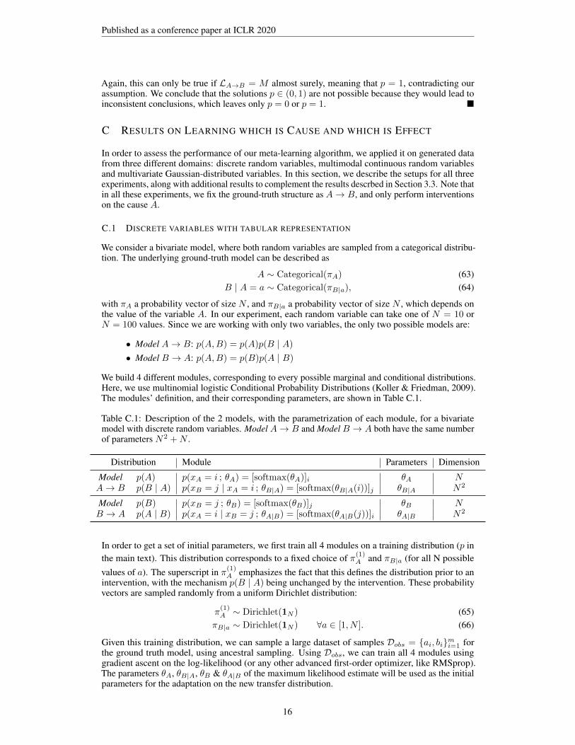
C RESULTS ON LEARNING WHICH IS CAUSE AND WHICH IS EFFECT

In order to assess the performance of our meta-learning algorithm, we applied it on generated datafrom three different domains: discrete random variables, multimodal continuous random variablesand multivariate Gaussian-distributed variables. In this section, we describe the setups for all threeexperiments, along with additional results to complement the results descrbed in Section 3.3. Note thatin all these experiments, we fix the ground-truth structure as A→ B, and only perform interventionson the cause A.

C.1 DISCRETE VARIABLES WITH TABULAR REPRESENTATION

We consider a bivariate model, where both random variables are sampled from a categorical distribu-tion. The underlying ground-truth model can be described as

A ∼ Categorical(πA) (63)B | A = a ∼ Categorical(πB|a), (64)

with πA a probability vector of size N , and πB|a a probability vector of size N , which depends onthe value of the variable A. In our experiment, each random variable can take one of N = 10 orN = 100 values. Since we are working with only two variables, the only two possible models are:

• Model A→ B: p(A,B) = p(A)p(B | A)

• Model B → A: p(A,B) = p(B)p(A | B)

We build 4 different modules, corresponding to every possible marginal and conditional distributions.Here, we use multinomial logistic Conditional Probability Distributions (Koller & Friedman, 2009).The modules’ definition, and their corresponding parameters, are shown in Table C.1.

Table C.1: Description of the 2 models, with the parametrization of each module, for a bivariatemodel with discrete random variables. Model A→ B and Model B → A both have the same numberof parameters N2 +N .

Distribution Module Parameters Dimension

Model p(A) p(xA = i ; θA) = [softmax(θA)]i θA NA→ B p(B | A) p(xB = j | xA = i ; θB|A) = [softmax(θB|A(i))]j θB|A N2

Model p(B) p(xB = j ; θB) = [softmax(θB)]j θB NB → A p(A | B) p(xA = i | xB = j ; θA|B) = [softmax(θA|B(j))]i θA|B N2

In order to get a set of initial parameters, we first train all 4 modules on a training distribution (p inthe main text). This distribution corresponds to a fixed choice of π(1)

A and πB|a (for all N possiblevalues of a). The superscript in π(1)

A emphasizes the fact that this defines the distribution prior to anintervention, with the mechanism p(B | A) being unchanged by the intervention. These probabilityvectors are sampled randomly from a uniform Dirichlet distribution:

π(1)A ∼ Dirichlet(1N ) (65)

πB|a ∼ Dirichlet(1N ) ∀a ∈ [1, N ]. (66)

Given this training distribution, we can sample a large dataset of samples Dobs = {ai, bi}mi=1 forthe ground truth model, using ancestral sampling. Using Dobs, we can train all 4 modules usinggradient ascent on the log-likelihood (or any other advanced first-order optimizer, like RMSprop).The parameters θA, θB|A, θB & θA|B of the maximum likelihood estimate will be used as the initialparameters for the adaptation on the new transfer distribution.

16


Similar to the way we defined the training distribution, we can define a transfer distribution (p̃ in themain text) as an intervention on the random variable A. In this experiment, this accounts for changingthe distribution of A, that is with a new probability vector π(2)

A , also sampled from a uniform Dirichletdistribution

π(2)A ∼ Dirichlet(1N ). (67)

To perform adaptation on the transfer distribution, we also sample a smaller transfer dataset Dint ={at, bt}Tt=1, with T � m. In our experiment, we used T = 20 datapoints, following the observationfrom Section 2.1.

C.2 DISCRETE VARIABLES WITH MLP PARAMETRIZATION

We consider a bivariate model, similar to the one defined in Appendix C.1, where each randomvariable is sampled from a categorical distribution. Instead of expressing the CPDs in tabular form,we use structured CPDs, parametrized with multi-layer perceptrons (MLPs). In our experiment, allthe MLPs have only one hidden layer with H = 8 hidden units, with a ReLU non-linearity, and theoutput layer has a softmax non-linearity. To avoid any modeling bias, we assume that the ground-truthmodel is also parametrized by MLPs, such that

A ∼ Categorical(MLP(0 ; WA)) (68)B | A = a ∼ Categorical(MLP(1[a] ; WB)) (69)

where 0 is a vector of size N will all zeros, and 1[a] is a one-hot vector of size N . WA and WB

summarize the parameters of the ground truth model, with the weights and biases for the 2 layers.Similar to the tabular representation, we define 4 different modules, this time using MLPs. Theirdefinition, as well as their corresponding parameters, are shown in Table C.2.

Table C.2: Description of the 2 models, with the parametrization of each module, for a bivariatemodel with discrete random variables, and MLP parametrization. Model A→ B and Model B → Aboth have the same number of parameters 3NH + 2(N +H).


Model p(A) p(xA = i ; θA) = [MLP(0 ; θA)]i θA NH +H +NA→ B p(B | A) p(xB = j | xA ; θB|A) = [MLP(1[xA] ; θB|A)]j θB|A 2NH +H +N

Model p(B) p(xB = j ; θB) = [MLP(0 ; θB)]j θB NH +H +NB → A p(A | B) p(xA = i | xB ; θA|B) = [MLP(1[xB ] ; θA|B)]i θA|B 2NH +H +N

Again, to define the training distribution, we first fix the parameters W (1)A and WB . We use randomly

initialized networks for the training distribution, with the parameters sampled using the He initializa-tion. We train all the modules using maximum likelihood on a large dataset of training samples Dobs,to get the initial set of parameters for the adaptation on the transfer distribution.

We also define a transfer distribution as the result of an intervention on A. In this experiment, thismeans sampling a new set of parameters W (2)

A , still as a randomly initialized network. We sample atransfer dataset Dint = {at, bt}Tt=1, with T = 20 datapoints.

C.3 CONTINUOUS MULTIMODAL VARIABLES

Consider a family of joint distributions pµ(A,B) over the causal variables A and B, defined by thefollowing structural causal model (SCM):

A ∼ pµ(A) = N (µ, σ2 = 4) (70)B := f(A) +NB NB ∼ N (0, 1), (71)

where f is a randomly generated spline, and the noise NB is sampled iid. from the unit Gaussiandistribution. To obtain the spline, we sample K points {xk}Kk=1 uniformly spaced from the interval[−8, 8], and another K points {yk}Kk=1 uniformly randomly from the interval [−8, 8]. This yields K

17


pairs {xk, yk}Kk=1, which make the knots of a second-order spline. We choose K = 8 points in ourexperiments.

The conditional distributions p(B | A) and p(A | B) are parametrized as 2-layer Mixture Den-sity Networks (MDNs; Bishop, 1994), with 32 hidden units and 10 components. The marginaldistributions p(A) and p(B) are parametrized as Gaussian Mixture Models (GMMs), also with 10components. The definition of the different modules, as well as their corresponding parameters, areshown in Table C.3.

Table C.3: Description of the 2 models, with the parametrization of each module, for a bivariatemodel with continuous multimodal variables. Model A→ B and Model B → A both have the samenumber of parameters 2,140.


Model p(A) p(xA ; θA) = GMM(xA ; θA) θA 30A→ B p(B | A) p(xB | xA ; θB|A) = MDN(xB , xA ; θB|A) θB|A 2,110

Model p(B) p(xB ; θB) = GMM(xB ; θB) θB 30B → A p(A | B) p(xA | xB ; θA|B) = MDN(xA, xB ; θA|B) θA|B 2,110

We select p0(A,B) as the training distribution, from which we sample a large dataset Dobs usingancestral sampling. Similar to the earlier experiments, this dataset is used to get the initial setof parameters for the adaptation on the transfer distribution. The MDNs are fitted with gradientdescent, while the GMMs are learned via Expectation Maximization. The transfer distribution is theresult of an intervention on A, where we shift the distribution pµ(A) with µ sampled uniformly in[−1, 1]. In Figure C.1, we plot samples from the training distribution (µ = 0), as well as two transferdistributions (µ = ±4).

−10 −5 0 5 10A

−12.5

−10.0

−7.5

−5.0

−2.5

0.0

2.5

5.0

B

Training

Transfer (µ = −4)

Transfer (µ = +4)

Figure C.1: Samples from the training (blue) and transfer (red and green) distributions, from an SCMgenerated with the procedure described above. The red datapoints are sampled from p−4(A,B), thegreen datapoints from p4(A,B), and the blue datapoints from p0(A,B).

The structural regret R(γ) is now minimized with respect to γ for 500 iterations (updates of γ).In the notation of Algorithm 1, these are the iterations over the number of episodes. Figure C.2shows the evolution of σ(γ) as training progresses. This is expected, given that we expect the causalmodel to perform better on the transfer distributions, i.e. we expect LA→B > LB→A in expectation.Consequently, assigning a larger weight to LA→B optimizes the objective (see Proposition 3).

Finally as a sanity check, we test the experimental set-up described above on a linear SCM withadditive Gaussian noise. In this setting, it is well known that the causal structure cannot be discoveredfrom observations alone Peters et al. (2017) and one must rely on the transfer distribution tell causefrom effect.

To that end, we repeat the experiment in Figure C.2 with the following amendments: (a) we replacethe non-linear spline with a linear curve (Figure C.3), and (b) in addition to training the structural

18



0.0

0.2

0.4

0.6

0.8

1.0

σ(γ

)

A B

A B

Figure C.2: Evolution of the sigmoid of the structural parameter σ(γ), with the number of episodes(meta-training iterations). The belief of A → B being the correct causal model increases as thenumber of episodes increases.

parameter by adapting the A→ B and B → A models to multiple interventional distributions, wetrain it by “adapting" the said model to the train distribution, where the latter serves as a baseline.

Figure C.4 shows that using multiple transfer (i.e. interventional) distributions (“With Interventions")enables causal discovery, as opposed to the model trained with a single observational distribution.This confirms that our method indeed relies on the interventional distributions to discover the causalstructure.

7.5 5.0 2.5 0.0 2.5 5.0 7.5 10.0X

10

5

0

5

10

Y

SCM Parameter = -4SCM Parameter = 0SCM Parameter = 4

Figure C.3: Samples from a linear SCM, showing training (orange) and two transfer distributions(blue and green).

C.4 LINEAR GAUSSIAN MODEL

In this experiment, the two variablesA andB are vector-valued, taking values in Rd. The ground-truthcausal model is given by

A ∼ N (µ,Σ) (72)

B := β1A+ β0 +NB NB ∼ N (0, Σ̃), (73)

where µ ∈ Rd, β0 ∈ Rd and β1 ∈ Rd×d. Σ and Σ̃ are two d × d covariance matrices. In ourexperiment, d = 100. Once again, we want to identify the correct causal direction between A and B.

19



0.2

0.3

0.4

0.5

0.6

0.7

0.8

0.9

1.0

() [

Mea

n ±

StdD

ev]

Without InterventionsWith Interventions

Figure C.4: Evolution of the sigmoid of the structural parameter σ(γ), with the number of episodes(meta-training iterations) in case of a linear model with additive Gaussian noise. The blue curvecorresponds to the setting where we make use of interventions, whereas the orange curve correspondsto one where we do not (i.e. use a single distribution). The shaded bands show the standard deviationover 40 runs (of both pre- and meta-training). We find (as expected) that causal discovery failswithout interventions but succeeds when transfer distributions are available.

To do so, we consider two models A → B and B → A parametrized with Gaussian distributions.The details of the modules’ definitions, as well as their parameters, is given in Table C.4. Note thateach covariance matrix is parametrized using the Cholesky decomposition.

Table C.4: Description of the 2 models, with the parametrization of each module, for a bivariatemodel with linear Gaussian variables. Model A→ B and Model B → A both have the same numberof parameters 2d2 + 3d.


Model p(A) p(xA ; θA) = N (xA | µA,ΣA) µA,ΣA d(d+ 1)/2 + dA→ B p(B | A) p(xB | xA ; θB|A) = N (xB |W1xA +W0,ΣB|A) W1,W0,ΣB|A 3d(d+ 1)/2

Model p(B) p(xB ; θB) = N (xB | µB ,ΣB) µB ,ΣB d(d+ 1)/2 + dB → A p(A | B) p(xA | xB ; θA|B) = N (xA | V1xB + V0,ΣA|B) V1, V0,ΣA|B 3d(d+ 1)/2

To build the training distribution, we draw µ(1), β0 and β1 from a Gaussian distribution, and Σ(1)

and Σ̃ from an inverse Wishart distribution. The transfer distribution is the result of an interventionon A, meaning that the marginal p̃(A) changes. To do so, we sample new parameters µ(2) from aGaussian distribution, and Σ(2) from an inverse Wishart distribution as well.

Unlike the previous experiments, we are not conduction any pre-training on actual data from thetraining distribution. Instead, we fix the parameters of both models to their exact values, according tothe ground truth distribution. For Model A → B, this can be done easily. For the Model B → A,we compute the exact parameters analytically using Bayes rule. This can be seen as the maximumlikelihood estimate in the limit of infinite data. In Figure C.5, we show that, after 200 episodes, σ(γ)converges to 1, indicating the success of the method on this particular task.

C.5 EXPERIMENTS WITH SOFT INTERVENTION

In this section, we describe an experimental setting where the conditional p(B | A) is perturbedwhile the distribution of the cause, p(A), is left unchanged. To that end, consider a set-up similar tothat in Section C.3:

20


Figure C.5: Convergence of the causal belief (to the correct answer) as a function of the number ofmeta-learning episodes, for the linear Gaussian experiments.

A ∼ pµ(A) = U(−8, 8) (74)B := f0(A) +NB NB ∼ N (0, 1), (75)

where f0 is a randomly generated spline and NB is sampled iid. from the unit Gaussian distributionand the cause variable A is sampled from the uniform distribution supported on [−8, 8].

To induce soft-interventions, we modify the SCM as follows. Consider the knots {ai, bi}5i=1 ofthe order 3 spline f0; we obtain a new spline fint by randomly perturbing the b-coordinate of theknots, where the perturbations are sampled from another uniform distribution1. Using the perturbedspline fint instead of f0 in Equation (74) results in a new SCM, from which we generate a singletransfer distribution (i.e. for a single episode). In Figure C.6 we plot samples from three such transferdistributions.

5 0 5A

10

5

0

5

10

B

Training SCMTransfer SCM

5 0 5A

B


5 0 5A

B


Figure C.6: Samples from different training (blue) and transfer (orange) distributions, from SCMsgenerated with the procedure described above, namely: all transfer SCMs (orange) are obtained bysoft-intervening of the underlying training SCM (blue).

The models used are identical to those detailed in Appendix C.3 and are trained on the trainingSCM (corresponding base-spline f0) with a large amount of samples (≈ 3,000k). The meta-trainingprocedure differs in that (a) in every transfer episode, we create a new spline fint and sample atransfer distribution Dint from the corresponding SCM, and (b) we use the following measure ofadaptation:

LG(Dint) = exp [log p(Dint | θ(T )G )− log p(Dint | θ(0)

G )] (76)where G is one of A→ B or B → A. The meta-transfer objective in Equation (5) remains the same.

Figure C.7 shows the evolution of the σ(γ) as the training progresses, and we find that the structuralparameter correctly converges to 1, representing the correct causal graph A→ B.

1The scale of the perturbation is 0.5 times that of the original knots.

21



0.6

0.7

0.8

0.9

1.0

() [

Mea

n ±

StdD

ev]

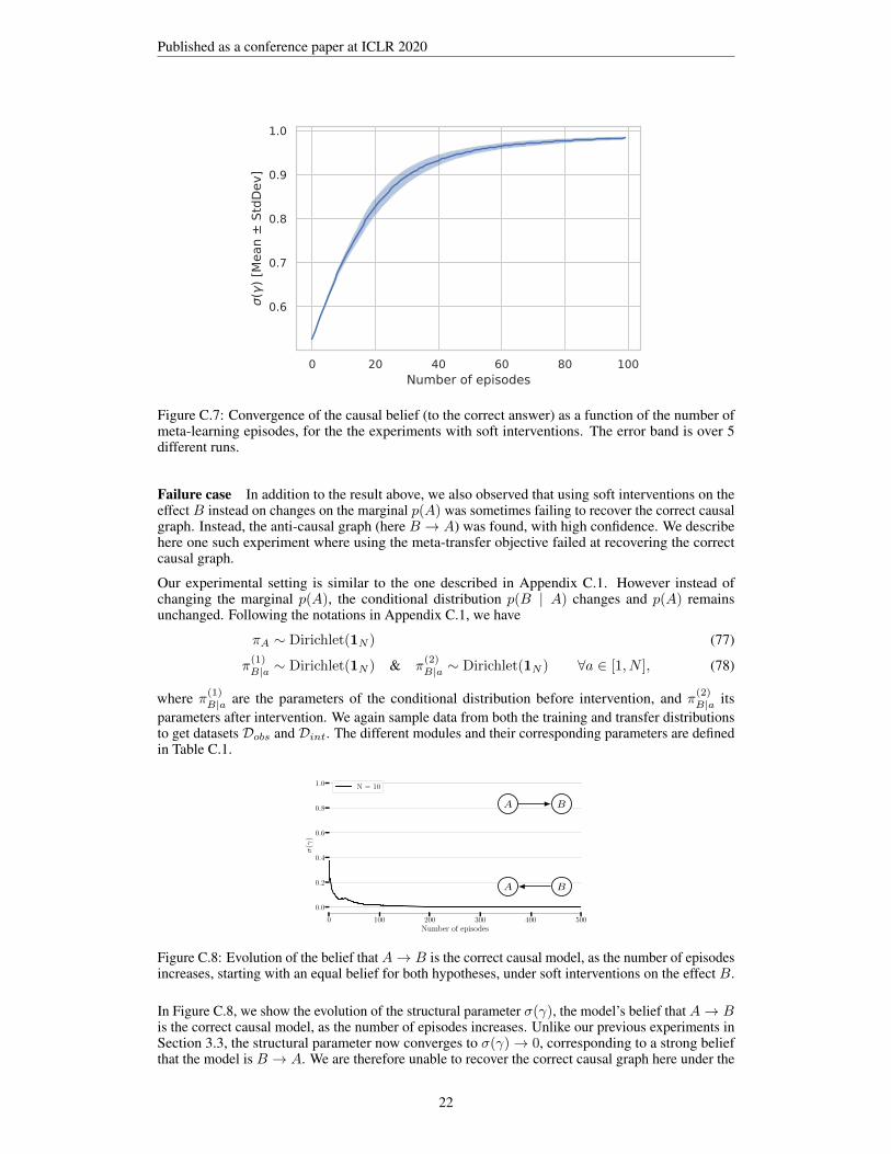
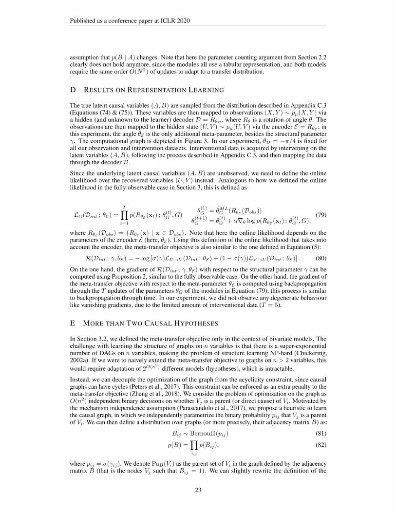
Figure C.7: Convergence of the causal belief (to the correct answer) as a function of the number ofmeta-learning episodes, for the the experiments with soft interventions. The error band is over 5different runs.

Failure case In addition to the result above, we also observed that using soft interventions on theeffect B instead on changes on the marginal p(A) was sometimes failing to recover the correct causalgraph. Instead, the anti-causal graph (here B → A) was found, with high confidence. We describehere one such experiment where using the meta-transfer objective failed at recovering the correctcausal graph.

Our experimental setting is similar to the one described in Appendix C.1. However instead ofchanging the marginal p(A), the conditional distribution p(B | A) changes and p(A) remainsunchanged. Following the notations in Appendix C.1, we have

πA ∼ Dirichlet(1N ) (77)

π(1)B|a ∼ Dirichlet(1N ) & π

(2)B|a ∼ Dirichlet(1N ) ∀a ∈ [1, N ], (78)

where π(1)B|a are the parameters of the conditional distribution before intervention, and π

(2)B|a its

parameters after intervention. We again sample data from both the training and transfer distributionsto get datasets Dobs and Dint. The different modules and their corresponding parameters are definedin Table C.1.


0.0

0.2

0.4

0.6

0.8

1.0

σ(γ

)

N = 10

A B

A B

Figure C.8: Evolution of the belief that A→ B is the correct causal model, as the number of episodesincreases, starting with an equal belief for both hypotheses, under soft interventions on the effect B.

In Figure C.8, we show the evolution of the structural parameter σ(γ), the model’s belief that A→ Bis the correct causal model, as the number of episodes increases. Unlike our previous experiments inSection 3.3, the structural parameter now converges to σ(γ)→ 0, corresponding to a strong beliefthat the model is B → A. We are therefore unable to recover the correct causal graph here under the

22


assumption that p(B | A) changes. Note that here the parameter counting argument from Section 2.2clearly does not hold anymore, since the modules all use a tabular representation, and both modelsrequire the same order O(N2) of updates to adapt to a transfer distribution.

D RESULTS ON REPRESENTATION LEARNING

The true latent causal variables (A,B) are sampled from the distribution described in Appendix C.3(Equations (74) & (75)). These variables are then mapped to observations (X,Y ) ∼ pµ(X,Y ) viaa hidden (and unknown to the learner) decoder D = RθD , where Rθ is a rotation of angle θ. Theobservations are then mapped to the hidden state (U, V ) ∼ pµ(U, V ) via the encoder E = RθE ; inthis experiment, the angle θE is the only additional meta-parameter, besides the structural parameterγ. The computational graph is depicted in Figure 3. In our experiment, θD = −π/4 is fixed forall our observation and intervention datasets. Interventional data is acquired by intervening on thelatent variables (A,B), following the process described in Appendix C.3, and then mapping the datathrough the decoder D.

Since the underlying latent causal variables (A,B) are unobserved, we need to define the onlinelikelihood over the recovered variables (U, V ) instead. Analogous to how we defined the onlinelikelihood in the fully observable case in Section 3, this is defined as

LG(Dint ; θE) =

T∏

t=1

p(RθE (xt) ; θ(t)G , G)

θ(1)G = θ̂ML

G (RθE (Dobs))θ

(t+1)G = θ

(t)G + α∇θ log p(RθE (xt) ; θ

(t)G , G),

(79)

where RθE (Dobs) = {RθE (x) | x ∈ Dobs}. Note that here the online likelihood depends on theparameters of the encoder E (here, θE ). Using this definition of the online likelihood that takes intoaccount the encoder, the meta-transfer objective is also similar to the one defined in Equation (5):

R(Dint ; γ, θE) = − log [σ(γ)LU→V (Dint ; θE) + (1− σ(γ))LV→U (Dint ; θE)] . (80)

On the one hand, the gradient of R(Dint ; γ, θE) with respect to the structural parameter γ can becomputed using Proposition 2, similar to the fully observable case. On the other hand, the gradient ofthe meta-transfer objective with respect to the meta-parameter θE is computed using backpropagationthrough the T updates of the parameters θG of the modules in Equation (79); this process is similarto backpropagation through time. In our experiment, we did not observe any degenerate behaviourlike vanishing gradients, due to the limited amount of interventional data (T = 5).

E MORE THAN TWO CAUSAL HYPOTHESES

In Section 3.2, we defined the meta-transfer objective only in the context of bivariate models. Thechallenge with learning the structure of graphs on n variables is that there is a super-exponentialnumber of DAGs on n variables, making the problem of structure learning NP-hard (Chickering,2002a). If we were to naively extend the meta-transfer objective to graphs on n > 2 variables, thiswould require adaptation of 2O(n2) different models (hypotheses), which is intractable.

Instead, we can decouple the optimization of the graph from the acyclicity constraint, since causalgraphs can have cycles (Peters et al., 2017). This constraint can be enforced as an extra penalty to themeta-transfer objective (Zheng et al., 2018). We consider the problem of optimization on the graph asO(n2) independent binary decisions on whether Vj is a parent (or direct cause) of Vi. Motivated bythe mechanism independence assumption (Parascandolo et al., 2017), we propose a heuristic to learnthe causal graph, in which we independently parametrize the binary probability pij that Vj is a parentof Vi. We can then define a distribution over graphs (or more precisely, their adjacency matrix B) as:

Bij ∼ Bernoulli(pij) (81)

p(B) =∏

i,j

p(Bij), (82)

where pij = σ(γij). We denote PaB(Vi) as the parent set of Vi in the graph defined by the adjacencymatrix B (that is the nodes Vj such that Bij = 1). We can slightly rewrite the definition of the

23


online-likelihood as in Section 3 to show the dependence on B:

LB(Dint) =

T∏

t=1

p(xt ; θ(t)B , B) =

n∏

i=1

T∏

t=1

p(x(t)i | x

(t)PaB(Vi)

; θ(t)B,i), (83)

where the second equality uses the factorization of p in the graph defined by B. Note that since thegraph defined by B can contain cycles, the definition in Equation (83) involves the pseudolikelihoodinstead of the joint likelihood (which is defined as the product of individual conditional distributionsonly if the graph is a DAG). The pseudolikelihood was shown to be a reasonable approximation of thetrue joint likelihood when maximizing the joint likelihood (which is performed here for adaptation;Koller & Friedman (2009)). Similar to the bivariate case, we want to consider a mixture over allpossible graph structures, but where each component must explain the whole adaptation sequence.We can generalize our definition of the regret as

R(Dint) = − logEB [LB(Dint)]. (84)

Note, however, that this expectation is over the O(2n2

) possible values of B, which is intractable.We can rewrite the regret in a more convenient form:Proposition 4. The regretR(Dint) defined in Equation (84) can be decomposed as

R(Dint) = −n∑

i=1

logEBi[LBi

(Dint)], (85)

where Bi is a row of the matrix B, and LBi(Dint) appears in the factorization of LB(Dint) in

Equation (83):

LBi=

T∏

t=1

p(x(t)i | x

(t)PaB(Vi)

; θ(t)B,i) (86)

Proof. Recall that LB(Dint) =∏i LBi

(Dint), so that we can rewrite the regret as follows:R(Dint) = − logEB [LB(Dint)] (87)

= − log∑

B

p(B)LB(Dint) (88)

= − log∑

B1

∑

B2

. . .∑

Bn

[ n∏

i=1

p(Bi)LBi(Dint)]

(89)

= − log

n∏

i=1

[∑

Bi

p(Bi)LBi(Dint)]

(90)

= −n∑

i=1

log∑

Bi

p(Bi)LBi(Dint) (91)

= −n∑

i=1

logEBi[LBi

(Dint)] (92)

�

The structural parameters, here, are the O(n2) scalars γij . Regardless of the intractability of theregret, we can still derive its gradient wrt. each γij . The following proposition provides a directextension of Proposition 2 to the case of multiple variables:Proposition 5. The gradient of the regretR(Dint) wrt. the structural parameter γij is given by

∂R∂γij

= σ(γij)− σ(γij + ∆ij), (93)

where ∆ij is the difference in log-likelihoods of two mixture candidates, conditioning on the variableVj

∆ij = log(EBi [LBi(Dint) | Vj ∈ PaB(Vi)])− log(EBi [LBi(Dint) | Vj /∈ PaB(Vi)]) (94)

24


Proof. To simplify the notation, we remove the explicit dependence on the transfer distribution Dintin this proof. Recall from Proposition 4 that the regret can be written as

R = −n∑

i=1

logEBi[LBi

]. (95)

Using a conditional expectation, it follows that for any i, j

EBi[LBi

] =∑

Bi

p(Bi)LBi(96)

= p(Bij = 1) ·∑

Bi|Vj∈PaB(Vi)

p(Bi | Bij = 1)LBi+ p(Bij = 0) ·

∑

Bi|Vj /∈PaB(Vi)

p(Bi | Bij = 0)LBi

(97)

= σ(γij) ·∑

Bi|Vj∈PaB(Vi)

p(Bi | Bij = 1)LBi + (1− σ(γij)) ·∑

Bi|Vj /∈PaB(Vi)

p(Bi | Bij = 0)LBi (98)

To simplify the notation, let us define E(1)ij and E

(0)ij the two conditional expectations of LBi ,

conditioned on whether or not Vj is a parent of Vi in B

E(0)ij =

∑

Bi|Vj /∈PaB(Vi)

p(Bi | Bij = 0)LBi = EBi [LBi | Vj /∈ PaB(Vi)] (99)

E(1)ij =

∑

Bi|Vj∈PaB(Vi)

p(Bi | Bij = 1)LBi= EBi

[LBi| Vj ∈ PaB(Vi)], (100)

so that Equation (98) can be written as

EBi[LBi

] = σ(γij)E(1)ij + (1− σ(γij))E

(0)ij . (101)

Note that neither E(0)ij nor E(1)

ij depend on the structural parameter γij . Therefore we can now easilycompute the gradient ofR wrt. γij only

∂R∂γij

= − ∂

∂γijlog(σ(γij)E

(1)ij + (1− σ(γij))E

(0)ij

)(102)

= − 1

EBi [LBi ]

(σ(γij)(1− σ(γij))

[E

(1)ij − E

(0)ij

])(103)

If we substract σ(γij) from this expression gives us

σ(γij)−∂R∂γij

=1

EBi [LBi ]

(σ(γij)

2E(1)ij + σ(γij)(1− σ(γij))E

(0)ij

+ σ(γij)(1− σ(γij))[E

(1)ij − E

(0)ij

] )(104)

=σ(γij)

EBi [LBi ]E

(1)ij = x (105)

Denoting the previous expression as x, we can also easily compute 1− x:

1− x =1− σ(γij)

EBi[LBi

]E

(0)ij (106)

Using the logit function σ−1(x) = log x1−x , we can conclude that

σ−1

(σ(γij)−

∂R∂γij

)= log

σ(γij)E(1)ij

(1− σ(γij))E(0)ij

(107)

= logσ(γij)

1− σ(γij)+ logE

(1)ij − logE

(0)ij (108)

= γij + ∆ij (109)

�

25


While Proposition 5 gives an analytic form for the gradient of the regret wrt. the structural parameters,computing it is still intractable, due to ∆ij . However, we can still get an effecient stochastic gradientestimator from Proposition 4, which can be computed separately for each node of the graph (withsamples arising only out of Bi, the incoming edges of Vi):Proposition 6. If we consider multiple samples ofB in parallel, a biased but asymptotically unbiased(as the number K of these samples B(k) increases to infinity) estimator of the gradient of the overallregret with respect to the meta parameters can be defined as:

gij =

∑k(σ(γij)−B(k)

ij )L(k)Bi∑

k L(k)Bi

, (110)

where the index (k) indicates the values obtained for the k-th draw of B.

Proof. The gradient of the regret with respect to the meta-parameters γi of node i is

∂R∂γi

= −∑Bip(Bi)LBi

∂ log p(Bi)∂γi∑

BiP (Bi)LBi

= −EBi

[LBi

∂ log p(Bi)∂γi

]

EBi[LBi

](111)

Note that with the sigmoidal parametrization of p(Bi),log p(Bi) = Bij log σ(γij) + (1−Bij) log(1− σ(γij)) (112)

as in the cross-entropy loss. Its gradient can similarly be simplified to∂ log p(Bij)

∂γij=

Bijσ(γij)

σ(γij)(1− σ(γij))−(1−Bij)

(1− σ(γij))σ(γij)(1− σ(γij)))

= Bij − σ(γij). (113)A biased, but asymptotically unbiased, estimator of ∂R/∂γij is thus obtained by sampling K graphs(over which the means below are run):

gij =∑

k

(σ(γij)−B(k)ij )

L(k)Bi∑

k′ L(k′)Bi

(114)

where index (k) indicates the k-th draw ofB, and we obtain a weighted sum of the individual binomialgradients weighted by the relative regret of each draw B

(k)i of Bi, leading to Equation (110). �

We can therefore adapt Algorithm 1 using the gradient estimate in Proposition 6 to update thestructural parameters γij , without having to explicitly compute the full regretR(Dint). In additionto the gradient estimate provided by Proposition 6, we can also derive a Rao-Blackwellized (Rao,1992; Blackwell, 1947) estimate of the gradient of the regret, based on the formulation derived inProposition 5.Proposition 7. Let {B(k)}Kk=1 be K binary matrices (corresponding to sample graphs), sampledfrom independent Bernoulli distributions depending on the structural parameters γij

B(k)ij

iid∼ Bernoulli(σ(γij)), (115)

and their corresponding likelihoods L(k)Bi

. A Monte-Carlo estimate of the log-likelihood difference∆ij in Equation (94) is given by

∆̃(K)ij = log

(1

|K(1)ij |

∑

k∈K(1)ij

L(k)Bi

)− log

(1

|K(0)ij |

∑

k∈K(0)ij

L(k)Bi

), (116)

where K(0)ij = {k ; B

(k)ij = 0} and K(1)

ij = {k ; B(k)ij = 1} are (disjoint) sets of indices k, depending

on the value of B(k)ij .

Based on this Monte-Carlo estimate of ∆ij , we can define an estimate of the gradient of the regretRwrt. the structural parameter γij by

∂̃R∂γij

= σ(γij)− σ(γij + ∆̃(K)ij ). (117)

26


F THE EFFECT OF ADAPTATION ON THE ONLINE LIKELIHOOD

Since we are using the online likelihood defined in Equation (3) as a measure of adaptation in ourmeta-transfer objective, it is reasonable to know if this measure is sound. To validate this assumption,we are running an experiment similar to the one described in Section 2.1 and Figure 1, using the sameexperimental setup on discrete variables described in Section 3.3. However, instead of measuring theraw log likelihood on a validation set, we report the online likelihood LG(Dint) for both models inFigure F.1. The online likelihoods are scaled by the number of transfer examples seen for visualization.Similar to Figure 1, we can see that the difference in online likelihoods for both models is mostsignificant on a small amount of data.

100 101 102 103 104

Number of examples

−5.50

−5.25

−5.00

−4.75

−4.50

−4.25

−4.00

−3.75

On

lin

eL

ikel

ihoodL ·→·(D

)

A→ B

B → A

Figure F.1: Adaptation to the transfer distribution (online likelihood on transfer examples, verticalaxis), as more transfer examples are seen by the learner (horizontal axis). The curves are the medianover 20,000 runs, with their 25-75th quantiles intervals. The dotted line is the asymptotic onlinelikelihood

27

Date post:	04-Apr-2022
Category:	Documents
Upload:	others
View:	2 times
Download:	0 times

A M -T OBJECTIVE FOR LEARNING TO DISENTANGLE C …

Documents