Date post: | 01-Sep-2018 |
Category: |
Documents |
Upload: | truongkien |
View: | 213 times |
Download: | 0 times |
A MACHINE LEARNING APPROACH TO FOLLOWINGTRACE PARTICLES IN TURBULENT FLOW
By
RANDEL ALLAN CROWE
A DISSERTATION PRESENTED TO THE GRADUATE COUNCIL OFTHE UNIVERSITY OF FLORIDA
IN PARTIAL FULFILLMENT OF THE REQUIREMENTS FOR THEDEGREE OF DOCTOR OF PHILOSOPHY
UNIVERSITY OF FLORIDA
1977
ACKNOWLEDGEMENTS
Deserving much of the credit for the completion of this work is,
of course, my advisor. Professor Gale E. Nevill. Often in dark times,
he gave me needed encouragement and guidance and has my most sincere
thanks. Others on my committee should be noted for their patience as
well as valuable suggestions. Dr. Kurzweg reviewed the fluid mechanics
aspects and Dt. Boykin the dynamics and modeling. Little could have
been accomplished in my graduate work without the very early support
and friendship of Dr. Hemp. Enduring the final push. Dr. Shaffer
has my deepest appreciation. Yet many others should also be included.
Surely, Professor E. Rune Lindgren, and his associates, Drs.
Elkins and Jackman whose project provided this problem, together with
Professor Roland C. Anderson who aided in the optical analysis, should
be recognized for providing unending assistance and counseling. Quietly
in the background are the members of the "MNDC, ' a local social group,
too numerous to mention individually, but all very supportive and there
when needed. Unusual was the serendipity and productivity of my con-
versations with Mickey Rogers. All words fail me when I try to express
my appreciation and admiration of my wife, Pat, who gave me incessant
drive and inspiration. To my parents as well as those mentioned and
unmentioned, I would like to express my everlasting gratitude and
indebtedness.
iii
TABLE OF CONTENTS
Page
ACKNOWLEDGEMENTS i^^
LIST OF FIGURES.^^
villLIST OF TABLES
ABSTRACT
CHAPTER
I INTRODUCTION 1
Scope of Work 1
Pertinent Background for the Particle Following
Machine ^
II THE TRACE PARTICLE TECHNIQUE AND DATA ACQUISITION SYSTEM.. 9
The Use of Trace Particles for Flow Visualization 9
Earlier Particle Following Approaches 10
Qualitative Observations of Particle Motion 14
III A PARTICLE FOLLOWING MACHINE 21
Overview •21
PFM: Input and Output 23
Image Path Attributes 26
Following Image Paths: The Decision Process 33
The Image Feature Vector 41
Modeling the Residual 44
Control of the PFM 53
Measuring Performance 54
Summary 56
iv
CHAPTER Page
IV PFM: INITIALIZATION AND IMPLEMENTATION 58
Initialization 58
The Data 66
The Initialization Program 69
The Particle Following Program 69
Program LEARN: Determination of the JointProbabilities 74
V RESULTS OF PERFORMANCE TESTS 76
Initialization 76
Particle Following 85
Performance of the PFP 90
VI DISCUSSION AND CONCLUSIONS 95
APPENDIX A ANALYSIS OF THE DATA ACQUISITION SYSTEM 98
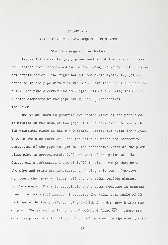
The Data Acquisition System 98
Approximate Geometric Ray Trace 104
Qualitative Observations of Images 107
Geometric Ray Trace 108
Spot Diagrams 128
Digitization of Film Data 133
Path Characteristics Using Orthogonal Projections.. 136
APPENDIX B APPROXIMATE GEOMETRIC RAY TRACE PRISM EQUATIONS 144
APPENDIX C TABLET DIGITIZER ERROR 155
APPENDIX D FORTRAN PROGRAM LISTINGS 164
BIBLIOGRAPHY 183
BIOGRAPHICAL SKETCH 187
LIST OF FIGURES
FIGURE Page
1-1 DATA ACQUISITION SYSTEM BLOCK DIAGRAM 3
2-1 THE DATA ACQUISITION SYSTEM 11
3-
1
THE PARTICLE FOLLOWING MACHINE 22
3-2 DIGITIZED IMAGE PLANE COORDINATES 22
3-3 IMAGE CANDIDATES AND ERRORS 35
3-4 LINK CLASSES, DECISION STATES AND HYPOTHESES 37
3-5 EXAMPLE OF JOINT TRANSITION PROBABILITY 49
3-6 BLOCK DIAGRAM OF THE PARTICLE FOLLOWING MACHINE 57
4-1 FRAME-BY-FRAME DATA 67
4-2 INVERTIBLE PATH DATA 67
4-3 SIMPLIFIED FLOWCHART OF "INIT" 70
4-4 SIMPLIFIED FLOWCHART OF "PFP" 71
4-5 SBIPLIFIED FLOWCHART OF "LEARN" 75
5 -1 TANGENTIAL AND NORMAL ACCELERATION COSTS 77
5-2 COST FUNCTION CONTOURS 79
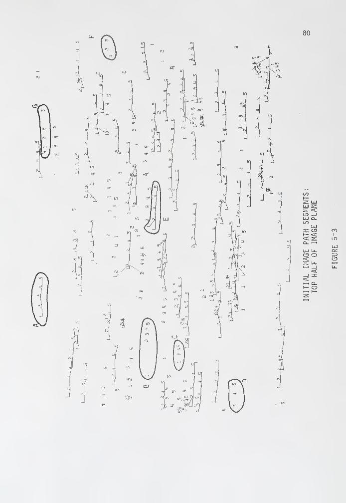
5-3 INITIAL IMAGE PATH SEGMENTS: TOP HALF OF IMAGE PLANE 80
5-4 INITIAL IMAGE PATH SEGMENTS: BOTTOM HALF OF IMAGE PLANE.. 81
5-5 RESIDUAL JOINT TRANSITION PROBABILITY, s = 1.0 86
5-6 RESIDUAL JOINT TRANSITION PROBABILITY, s = 1.2 87
5-7 RESIDUAL JOINT TRANSITION PROBABILITY, s = 1.5 88
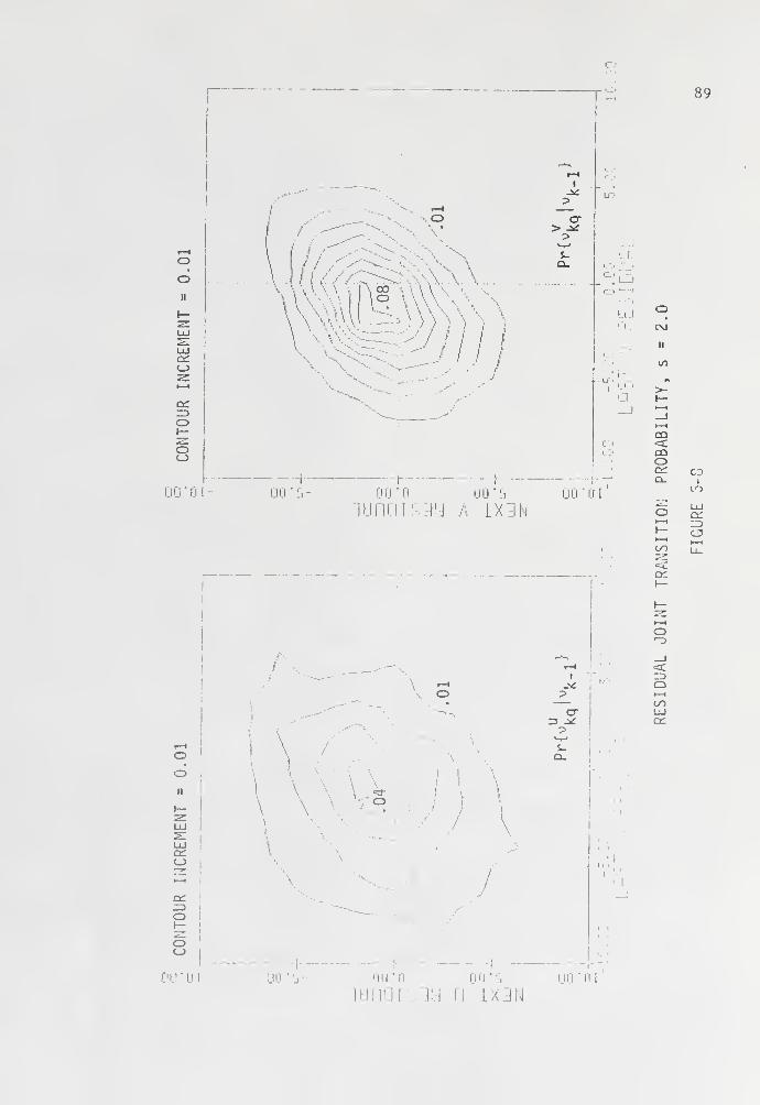
5-8 RESIDUAL JOINT TRANSITION PROBABILITY, s = 2.0 89
A-1 DEFINITION OF COORDINATE AXES 99
A-2 APPROXIMATE MERIDIONAL RAY TRACE 106
VI
FIGURE Page
A-3 GRID OF OBJECT POINTS 109
A-4 MERIDIONAL RAY TRACE: LARGE PRISM 110
A-5 OFF-AXIS RAY TRACE: LARGE PRISM 110
A-6 RAY TRACE TOP VIEW Ill
A-7 PRINCIPAL RAYS FROM OBJECT GRID INTERSECTING IMAGE PLANE.. Ill
A-8 MERIDIONAL RAY TRACE : SMALL PRISM 113
A-9 LARGE PRISM RAY LENGTHS FOR FULL LIGHTING 115
A-IO UNNECESSARY CONFUSION FOR LARGE PRISM WITH FULL LIGHTING.
.
115
A-11 SMALL PRISM RAY LENGTHS FOR FULL LIGHTING 116
A-12 UNNECESSARY CONFUSION FOR SMALL PRISM WITH FULL LIGHTING.
.
116
A-13 LIGHTING SCHEMES 117
A-14 UNNECESSARY CONFUSION FOR HALF AND CIRCLE ILLUMINATION 118
A-15 VOLUME SENSITIVITIES (cm^/mm'^) 123
A-16 PROBABILITIES FOR CONFUSION AND OVERLAP 124
A-17 HEXAPOLAR ARRAY 130
A-18 OBJECT POINT LOCATIONS 130
A-19 SENSITIVITY OF FOCUSING POINT A 131
A-20 SPOT DIAGRAMS FOR POINT A AND A' , BEST FOCUS 132
A-21 SPOT DIAGRAMS FOR POINT C AND C, BEST FOCUS SET FORPOINT A 134
A-22 SPOT DIAGRAMS FOR POINTS B AND B' , BEST FOCUS ON A 135
A-23 ORTHOGONAL STEREOSCOPIC PROJECTION OF A PATH 137
B-1 RAY TRACE GEOMETRY 146
C-1 DISTRIBUTION OF PEN LOCATION ABOUT DESIRED IMAGE
LOCATION 156
C-2 TWO DIMENSIONAL REGIONS 156
Vll
LIST OF TABLES
TABLEPage
5-1 KEY TO FIGURES 5.3 AND 5.4 82
5-2 INITIALIZATION PERFORMANCE ON 207 FRAME-ONE IMAGES 84
5-3 PFP PERFORMANCE, s = 2.0^2
5-4 ISOLATION OF DECISIONS^^
A-la APPROXIMATE PARTICLE MOVEMENT (MM) IN SHUTTER TIME 103
A-lb APPROXIMATION USING MAX VELOCITY= UBARvO. 791 103
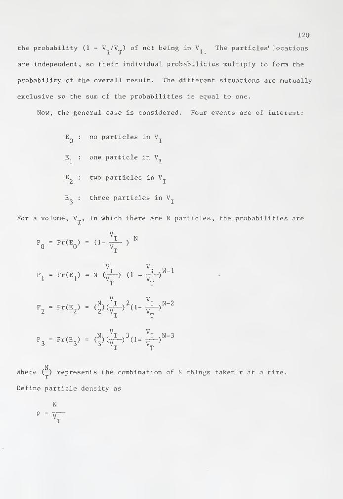
A-2 PROBABILITY OF TWO PARTICLES OCCURRING IN Vj 119
A-3 AVERAGE CONFUSION AND OVERLAP PROBABILITIES FOR SMALL^^^^^
126
A-4 AVERAGE CONFUSION AND OVERLAP PROBABILITIES K)R LARGE^^^^"
127
C-1 TWO DIMENSIONAL TABLET ERROR^^j^
C-2 PROBABILITY OF BIT ERROR FOR GIVEN E. 162
viii
Abstract of Dissertation Presented to the Graduate Councilof the University of Florida in Partial Fulfillment of the
Requirements for the Degree of Doctor of Philosophy
A MACHINE LEARNING APPROACH TO FOLLOWINGTRACE PARTICLES IN TURBULENT FLOW
By
Randel Allan Crowe
August 1977
Chairman: Gale E. Nevill, Jr.Major Department: Engineering Sciences
Machine learning is used in a statistical decision theoretic scheme
to follow trace particles in turbulent flow. Data used to demonstrate
performance came from previous experiments studying turbulent flow in a
pipe (Reynolds number less than 6500) , and consisted of digitized stereo-
scopic trace particle image locations. Accuracy of the data acquisition
technique is examined with emphasis on optical errors. Particle
location in the pipe is determined from its two stereo images. How-
ever, high trace particle count prevents immediate pairing of particle's
stereo images. Therefore, identification of image paths (sequentially
sampled particle locations) is carried out separately in each view.
The particle following scheme is initialized by short image path segments
found using search procedures based on finding five-image sequences with
minimum velocity variation. Image dynamics are modeled using a constant
acceleration assumption. An image's dynamic state is estimated using
a Kalman filter with finite fading memory. The next image belonging
to the path is sought in the neighborhood of a prediction. A minimum
error rate Bayes decision rule is applied to choose the next image
from the candidates in the neighborhood. The feature vector is
ix
composed of the two most recent filter residuals. Probabilities of
the residual transitions are learned by analyzing previously completed
and verified sequences. It is found that this scheme gives better
performance than earlier attempts, which utilized a constant velocity
assumption, including improved handling of image overlap, confusion,
and measurement noise. It is concluded that a semiautomated system
is necessary where the particle following procedure's output is.
verified by an operator who can change or correct decisions made.
CHAPTER I
INTRODUCTION
Scope of Work
Turbulence has evaded detailed and complete understanding by scores
of scientists over many generations. Recent attempts at its description
suffer from the difficulty of obtaining good experimental verification
which is needed in any modeling effort. In particular, two separate
experiments that have been reported utilized trace particles to facilitate
the detailed quantitative description of the structure of turbulence in
pipes. Johnson (1974) and Jackman (1976) used neutrally buoyant particles
in water and a novel prism-cinematographic data recording system to
study transition and low Reynolds number flows (3500 ^ Re ^ 6500).
Breton (1975) used small glass spheres in trichloroethelyne (TCE)
and a unique "distributed camera" system to study a flow with Reynolds
number of the order of 100,000. These workers were interested in a
Lagrangian description of the turbulence. That is, a turbulent model
written in terms of the individual traces of fluid elements. These
experiments generated stereoscopic film records of temporally sampled
particle paths, and both suffered from the Inability to automatically
reduce these data to the individual path sequences.
*This consisted of two sets of twenty lenses placed along a test sectionof the pipe.
Quantitative flow visualization requires taking data by an optical
system that records two different views (stereo views) of the particles
in the flow. Each view is a projection of the three-dimensional par-
ticle paths onto a two-dimensional film plane. By measuring the image
locations in the film plane, the two views of a particle can be used to
determine its three-dimensional position. This is what is termed photo-
grammetry. Breton (1975) used a sufficiently small number of particles
to allow straightforward determination of stereo pairs. Johnson (1975)
and Jackman (1976), however, had high particle counts making the immedi-
ate determination of stereo image pairs impossible. Instead, they deter-
mined the two-dimensional image paths ( a process called particle following)
of all images and then compared the paths to determine which were stereo
pairs (conjugate paths). A high particle count yields a better and more
reliable visualization. But the use of more particles increases the
burden on the data reduction procedures. Breton (1975) and Jackman (1976)
used automated procedures as much as possible but were not successful at
attaining full automation. Automatic data analysis is difficult and will
not become a reality without a thorough understanding of the data
acquisition system, its errors, the particle path characteristics and
the concepts of particle following. The work presented here considers
Jackman' s experimental arrangement and the errors in his data acquisition
system. Considered in detail is the particle following problem.
Data reduction consists of several identifiable subproblems which,
together, form a linear data acquisition and reduction system (See
Figure 1-1), Once the experimental system has been defined, the first
problem is to acquire quality stereo images of the trace particles.
[EXPERIMENTALAPPARATUS
OPTICS
IMAGE RECORDINGDIGITIZATION
PARTICLE FOLLOWINGMACHINE
IDENTIFYING CONJUGATE PATHS
TRANSFORM IMAGE PATHSINTO THREE DIMENSIONAL
SAMPLED PATHS
VISUALIZATIONAND
MODEL EVALUATION
DATA ACQUISITION SYSTEM BLOCK DIAGRAM
FIGURE 1-1
This is £in acute optics problem in the case of Johnson's (1975) prism
system. The present work includes an In depth analysis of the optical
properties of the pipe and prism system. Appendix A presents details of
the analysis. Second, the images must be recorded on film and their lo-
cations digitized for use by the analysis programs. Jackman's (1976)
use of a graphic tablet system for data entry is treated in Appendix C.
The primary concern of this work is the third step; converting the
digitized film data into image paths. The approach taken here involves
three procedures: prediction, decision making, and learning. The
combination of these processes to perform the image following task is
termed the Particle Following Machine (PFM) . The PFM takes the digitized
image locations and determines which images represent the same particle
from frame to frame (sample to sample) . It outputs image paths which can
be compared to find the conjugate paths. Then, a transformation is used
to determine the three-dimensional particle paths. These last two aspects
of the data analysis are not considered in the current work but they are
discussed along with the actual evaluation of the results in terms of
fluid turbulence theory by Johnson (1974), Breton (1975), and Jackman (1976),
The principal contribution of this work is the development of a
theoretical basis for the PFM. This approach to following images of
trace particles makes use of a combination of estimation, decision and
pattern recognition theory. The PFM is presented in a general format
and could be applied to other problems where a group of identical objects
are being tracked and the motion of an object is fairly consistent over
time. Performance tests of a specific implementation of the PFM were
made using a computer code written in FORTRAN. Some modifications would
be necessary to make this implementation an economic production program.
5
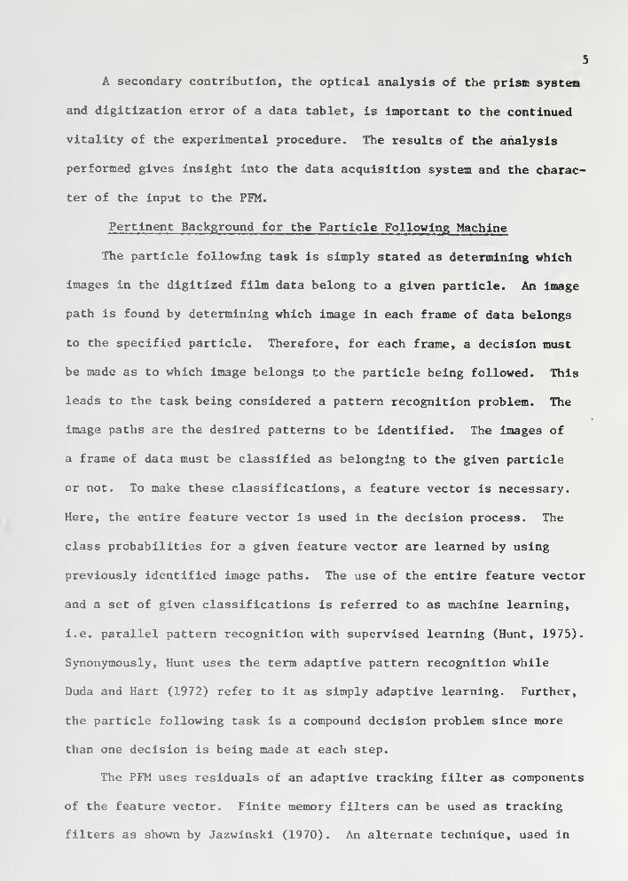
A secondary contribution, the optical analysis of the prism system
and digitization error of a data tablet, is important to the continued
vitality of the experimental procedure. The results of the analysis
performed gives insight into the data acquisition system and the charac-
ter of the input to the PFM.
Pertinent Background for the Particle Following Machine
The particle following task is simply stated as determining which
images in the digitized film data belong to a given particle. An image
path is found by determining which image in each frame of data belongs
to the specified particle. Therefore, for each frame, a decision must
be made as to which image belongs to the particle being followed. This
leads to the task being considered a pattern recognition problem. The
image paths are the desired patterns to be identified. The images of
a frame of data must be classified as belonging to the given particle
or not. To make these classifications, a feature vector is necessary.
Here, the entire feature vector is used in the decision process. The
class probabilities for a given feature vector are learned by using
previously identified image paths. The use of the entire feature vector
and a set of given classifications is referred to as machine learning,
i.e. parallel pattern recognition with supervised learning (Hunt, 1975).
Synonymously, Hunt uses the term adaptive pattern recognition while
Duda and Hart (1972) refer to it as simply adaptive learning. Further,
the particle following task is a compound decision problem since more
than one decision is being made at each step.
The PFM uses residuals of an adaptive tracking filter as components
of the feature vector. Finite memory filters can be used as tracking
filters as shown by Jazwinski (1970). An alternate technique, used in
the present work is the finite fading memory filter of Tarn and
Zaborszky (1970) . These filters are successful at tracking because
they eliminate possible divergence of the Kalman filter. The divergence
of the Kalman filter is considered by Price (1968) . Adaptive radar
tracking systems following manned maneuvering targets use similar track-
ing filters. Singer (1970) uses a Kalman filter to track targets with
known maneuvering capabilities. Singer and Behnke (1970) present a
comparison of five tracking filters concluding that the Kalman filter
requires the most computation but provides measures of tracking error
statistics. McAulay and Denlinger (1973) present a tracking filter
that tracks by changing its dynamic model of the target when a maneuver
is detected. This system requires knowing a target's allowed maneuvers
beforehand. Adaptive Kalman filters are treated in Gelb (19 74). Back-
ground on learning and adaptive systems can be found in Tsypkin (1971
and 1973). The general area of adaptive systems is scanned by Lainiotis
(1976).
Since the feature vector is constructed from filter residuals, it
is a time series. It is assumed here to be a Markov process with the
next state only dependent on the immediately previous state. This
use of the history of the feature vector makes the PFM an example of
making decisions in the context of the current situation (i.e. the way
the system got to its current state is important). Modeling the fea-
ture vector is then partially involved with time series analysis (Box
and Jenkins, 1970, and Robinson, 1967) and partially estimation theory
(Jazwinski, 1970).
7
The most interesting aspect of the PFM is its need to first
decide which image in a frame belongs to the particle being followed.
Once this decision has been made, normal estimation theory applies, i.e.
the last estimate can be updated with information from the next measure-
ment. The particle following task is therefore a combination of appli-
cations of decision theory and estimation theory. No directly applicable
literature was found that discussed the underlying theory of such a
system. This unique problem, then, requires as basic a development
as possible to provide a foundation on which to build a viable production
system. This is evident from the lack of success of other attempts
at automatic patticle following. Breton (1975) avoided the problem
entirely by resorting to manual entry of conjugate images and having a
very low particle/image density. Jackman (1976) tried to use a deter-
ministic approach that assumed constant velocity particles and no
measurement noise. This effectively reduced the amount of decision
making, but when a choice had to be made, it was arbitrary. Its per-
formance was fairly poor and the images were eventually followed by
manual effort. Since the desired image paths are known to be subsets
of the data (collections of images), one approach might be to test all
image combinations with a heuristic cost function. It would then
be assumed that paths with minimum cost would be the desired image
paths. With the image density that Jackman used, the number of
possible combinations is very large; at ten times the density, the
problem would be enormous. Nilsson (1971), and Newell and Simon (1972)
discuss heuristic problem solving. For this approach, the search of
possible combinations is heuristically guided by rules that "seem"
8
appropriate. These rules are ad-hoc but possibly simpler than the
decision theoretic approach taken here. It is difficult to base such
rules on theory and, typically, they provide neither Insight to their
accuracy nor guidance for their Improvement. The heuristic approach
is useful in solving the initialization problem. (See Chapter IV.)
Initially, there is no information available as to the dynamic state
of an image. By severly limiting the search and accepting some error,
a heuristic approach is taken to identify short image paths. These
initial path segments are then sufficient to start the particle following
procedure. Application of this initialization procedure to the particle
following task would ignore much information that is readily available
such as image state and measurement noise.
After a brief description of the data acquisition system and a
discussion of some aspects of the analysis of the optical system in
Chapter II, the PFM is described in Chapter III. Chapter IV presents
the details of initialization and programming a specific implementation
of the particle following machine while results and conclusions are
presented in Chapters V and VI respectively.
CHAPTER II
THE TRACE PARTICLE TECHNIQUE AND DATA ACQUISITION SYSTEM
Presented in this chapter is the background of the trace particle
technique and data acquisition system used by Johnson (1974) and
Jackman (1976). In addition, results of qualitative and quantitative
analyses of the system are discussed. These results provide a foundation
for the development of the particle following machine in Chapter III.
Details of the analysis are given in Appendix A.
The Use of Trace Particles for Flow Visualization
There exist numerous techniques for flow visualization. Their
purpose is to reveal the motion of a fluid element over time in com-
plicated flows. Additives such as dye, wax and rosin spheres, dust,
hydrogen bubbles, aluminum powder and mica flakes have all been tried.
Ideally, the trace material used follows the fluid motion precisely
without altering the flow structure by its presence. Examples of flow
visualization may be found in Reynolds (1883), Prandtl (1904), Page and
Townend (1932), Prandtl and Tietjens (1934), Lindgren (1954-1969), Coles
(1965), Kline et_ al (1967), Corino and Brodkey (1969), Kim et _al. (1971) ,
Johnson (1974), Breton (1975), Jackman (1976), Johnson et al. (1976), and
Elkins _et _al. (1977).
The use of pliolite trace particles is due to Nychas, Hershey, and
Brodkey (1973). These particles are desirable because they are opaque
(reflect light well), of selectable size, and almost neutrally buoyant.
Johnson (1974) gives a lengthy argument as to their abilities to follow
the fluid motion faithfully.
9
10
Johnson (1974) introduced the use of a prism to generate the stereo
images required for quantitative measurements. This technique requires
only one camera, simplifying somewhat the required equipment compared
to the special distributed camera of Breton (1975).
Quantitative descriptions are typically not obtainable from flow
visualization techniques due to the complicated equipment and analysis
required. Breton (1975) traced only a few particles compared to Johnson
(1974) . Jackman (1976) was able to attain one or two particles per cubic
centimeter which approaches a reasonable particle count (henceforth re-
ferred to as density). A goal of the current work of Lindgren and his
associates is to increase the density by an order of magnitude (Lindgren,
1977). As the density is increased, the work required in data reduction
increases tremendously and fully or semiautomatic procedures are vital.
Johnson performed all particle following by hand. Jackman was able to
develop semiautomated data entry, and path matching (finding conjugate
paths) procedures but resorted to following the images manually. Breton
reported failure of his automatic system to follow image path pairs and
essentially used a machine-assisted manual entry procedure.
The present work is a study of the particle following problem.
In order to understand the basis for the development of the particle
follower, the experimental system and data acquisition equipment need
to be understood. The remainder of Chapter II describes the apparatus
and discusses the results from analysis of the optical system.
Earlier Particle Following Approaches
Of primary concern to the current work is the data acquisition
system used by Jackman. Mounted at the observation station of his
experimental apparatus is a 90° prism as shown In Figure 2-1. Light
12
projected dovm the pipe reflects off the trace particles making them
highly visible. An observer looking into the pipe through the prism
sees two views of the particles in the pipe, one view in each of the
two prism faces. A particle is invertible if it has an image in both
views. Its location inside the pipe can then be calculated. The
region for which a particle's images are invertible depends on the
prism parameters, the pipe parameters, and the observer's position.
To enhance the capability of the system, two prisms were used. The
smaller is appropriate for studies of motion close to the wall; the
larger to make observations deep into the pipe. A Bell and Howell
35mm movie camera was used to record the particle images. Its film
rate was adjusted to suit the flow rate (faster flows—more particle
motion— faster film rate required). Two small light sources mounted
on the prism were used as reference points for frame alignment during
subsequent data conditioning and analysis. The display of a Hewlett
Packard digital counter was also recorded on each frame to allow
accurate determination of the sample rate.
Jackman used a graphic tablet digitizer to encode the image lo-
cations. The graphic tablet system consisted of a Scriptographics
Tablet Digitizer connected on-line to a Tektronix graphic terminal
interfaced to a central IBM 370/165 computer facility. Using a photo-
graphic enlarger, the film of a turbulent flow (Re=3500) was projected
onto the eleven-inch square tablet surface. The particle images were
then entered one-by-one using the tablet's locator pen. The images,
once encoded, were translated and rotated to a reference position by
use of the frame's reference points. His data consisted of 55 frames
13
and roughly 13,000 points whose entry into the computer through the
tablet was straightforward but tedious and highly susceptible to
operator error. Graphic output was used to verify data and quickly
showed most needed corrections. Once the image paths were identified
(manually), FORTRAN programs were used to find conjugate paths (particle
paths seen through both prism faces) . More processing yielded the three-
dimensional particle paths. (Jackman found approximately 150 pairs of
invertlble image paths. Breton's system made all images invertible,
but he used only 10-20 particles.) Use of the computer greatly reduced
the time used for data analysis; from the many months that Johnson*
used to a matter of hours. The procedures established by Jackman were
faster, but required a great deal of human-computer interaction for
data entry and manual particle following.
Jackman 's attempted but abandoned automatic particle following
procedure estimated the location of the next image from the last two
by assuming the particle's velocity constant and the measurement per-
fectly accurate. A window was constructed around the estimate and
the next image of a path was sought in this region. This was a straight-
forward, deterministic approach, yet it failed to follow particle paths
for a significant distance and made many errors in assigning an image
Johnson mounted the film as slides and using a standard projector,enlarged film records of a Re=6500 turbulent flow onto graph paper.He then recorded by hand the particle images' locations, and manuallydetermined the motion in time of each image path.
14
to its correct path. As is evident from this (and has been known to
researchers in computer vision for a long time) programming a machine
to do even as simple a human task as merging points into lines is not
easy. If frames are superimposed, the particle paths are immediately
evident to a human observer, yet to program a machine to find these
correct paths is not elementary.
Qualitative Observations of Particle Motion
There are a number of useful qualitative observations pertinent
to the discussion of the data acquisition system and image path at-
tributes. Direct observation of turbulence for Reynolds numbers from
3500 to 6500 was performed to obtain the following information. The
system was designed to study particle motion using a Lagrangian or
referential description of fluid flow. That is, motion of the fluid
elements is being observed which is strikingly different from more
common fluid flow descriptions using Eulerian or spatial descriptions.
For flows in the pipe, a strong axial velocity exists so that particles
neither back up nor traverse circles. The observer is given a feeling
of circular fluid motion, but if any specific particle is followed, none
is seen. Furthermore, particles are not observed (by the eye) to have
any random "jumpy" motion as is the case in Brownian motion and their
paths are seen to be smooth trajectories, typically of small curvature.
(Meant here is the curvature in the projection; the three-dimensional
curvature is nearly Impossible to observe since the particle's stereo
image and hence location in the pipe is not known.)
Particles are observed throughout the field of view to have widely
different speeds with faster particles giving the effect of being deeper
in the pipe. Bright, slowly-moving particles can sometimes be paired
15
to their stereo image. Observation of these shows that the motions
of the two stereo images are not particularly similar.
At low Reynolds numbers, large periods of laminar flow are seen.
Here, as expected, particles travel in paths parallel to the pipe
axis; slow particles near the wall, faster particles in the center.
As the Reynolds number is increased through transition, regions of
disturbed motion become more frequent. This turbulence occurs for
isolated periods and is referred to as a slug flow. As a turbulent
slug approaches the viewing station, observed particles begin to deviate
from their laminar trajectories with increasing violence of motion
until the slug has passed, when a sudden calming occurs. Observation
of particle paths at a higher Reynolds number (Re=4500) shows that the
projected paths vary in direction over time, smoothly, not erratically,
with at most 10 to 15 degrees of slope. This can be expected to in-
crease for higher Reynolds numbers but it does indicate how dominant
the mean velocity is.
These observations imply that following images should be straight-
forward since the expected paths are smooth and slowly changing. This
is not the case however. With Jackman's data, one major problem was the
large measurement noise incurred with the use of the tablet for data
entry and too few references for frame alignment. As the optical analy-
sis shows, there are other significant errors (See Appendix A).
There are errors due to the pipe-prism refractive properties,
perspective, camera imperfections, and particle movement. It is shown
in Appendix A, that during the exposure time, a particle may move on
the order of one millimeter in the pipe. This causes elongation of the
16
particle images and a loss of accuracy in the position of their center.
This error has been eliminated from future experiments by the use of
a strobed lighting system synchronized to the camera (Lindgren, 1977).
In addition, coma, caused by use of too low an f number on the camera
lens can be corrected by increasing the f number. This requires more
illumination which has been increased to some extent. An increased
f number also reduces the effect of astigmatism due to the pipe and
prism. The spot diagrams in Appendix A demonstrates the focusing
problems typical of astigmatism. A larger f number has a greater depth
of field bringing more of the pipe into focus and keeping the image size
small. Other errors are more significant.
Determining the location of a particle from the location of its
two stereo images requires transforming the image locations into inter-
secting rays in the pipe. Both Johnson and Jackman wrote analytic
approximations that were adequate in a region near the meridional
plane. A full three-dimensional analysis requires an iterative tech-
nique to determine a ray's direction and is therefore much more compli-
cated than the straightforward "prism equations" given in Appendix B.
It reveals that considerable error can occur in a particle's position
when using these approximations. This error increases as the camera
is moved closer to the pipe. The camera cannot be too far from the
pipe because the illumination is not adequate to sufficiently expose
the film at the film rate required and the lenses available. Thus,
full three-dimensional analysis is necessary. The close proximity
of the camera and the pipe causes this perspective problem. It also
causes another error. When projecting a line parallel to the pipe
17
axis into the image plane, the two stereo images are not scaled the
same, i.e. the foreshortening of the two images is different. This
causes sampled image locations of the two image paths not to be above
one another, increasing the difficulty of finding stereo image pairs.
Perspective errors are obscured in Jackman's data because of the large
measurement noise. As the system is improved and measurment noise
reduced, they will become more important and if not considered, will
reduce the capabilities of the data acquisition system.
There are other problems intrinsic to systems using projections.
The process of projecting the three-dimensional images onto an image
plane causes a loss of Information. Two such projections are required
just to recover the three-dimensional position of the particle. When
many particles are involved, images overlap and particles shadow
other particles. Stereo pairs of images cannot be readily identified.
A particle following machine must handle these phenomena to achieve a
reasonable performance level. The statistical approach taken in
Chapter III requires knowledge of the probability of occurrence of
these problems. In particular, two separate situations need to be
considered: overlap and confusion.
Overlap occurs when a particle comes between the camera and anoth-
er particle deeper in the pipe. Since the optical system has a finite
resolution, there is a region, something like a shadow, that exists for
each particle in which a second particle will be overlapped. This region
varies in size and shape depending on the particle's location. Any
particle In the shadow of another particle cannot be resolved by the
data acquisition system. If the two particles' images overlap only
18
partially, the center of the resultant image does not represent the
true location of either image and an error will be incurred when the
location of this image is digitized. This problem will always occur
for a system with finite resolution and must be considered in any error
analysis. In qualitative observations, the overlap of particles was
observed infrequently. As the particle density is increased, overlaps
can be expected to increase in occurrence. It can be concluded that
this "instrumentation" noise will always exist, perturbing the true
locations of the images.
Confusion is the term applied to the occurrence of images existing
near each other in the film plane even though their respective particles
may not be close to each other in the pipe. This is a result of the
projection of three-dimensional locations into two dimensions. There
are two types of confusion: necessary and unnecessary. Necessary
confusion occurs when invertible paths (particle paths with two image
paths) have images at a given time located in the same region. This
cannot be avoided. Unnecessary confusion occurs when paths that are
not invertible (paths with only one image path and hence not resolvable
into their three-dimensional positions) have images which occur in
the neighborhood of an invertible image. This problem can be corrected
to some extent by limiting the illumination in the pipe to a volume
that can be resolved by the prism (only invertible images are produced).
Of course, images occurring in the same region but at different times
cause no problems. Confusion cannot be observed directly since the
individual projections give no information as to particle location;
any image could possibly belong to an invertible particle.
19
In summary, the possibility of overlap means that image locations
cannot be considered as perfectly accurate, some measurement noise will
always exist. The fact that confusion will always occur to some extent
means that image paths may not necessarily be considered isolated. There-
fore, it cannot be assumed that a small window drawn around an image
that is larger than the system resolution will contain only one image.
This has implications about any image following scheme. If an estimate
is made of an image location, no matter how small a variance this esti-
mate may have, it is possible that other than the correct image is
arbitrarily close to the estimate. Hence, no estimator can "isolate"
a path, i.e. a decision as to which image is correct will always have
to be made. Finally, to make matters worse, both of these problems
increase in severity as particle density increases. The analysis in
Appendix A shows that data collected by Jackman can be considered
relatively sparse. He had a particle density on the order of one
particle per cubic centimeter. The probabilities of overlap and con-
fusion for this case are very small and allow the data to be reduced
even with the large measurement noise. Higher densities would have
less chance of being reduced correctly and hence would require a smaller
particle density or a smaller illuminated region. The sparse nature
of the data explains why it can be reduced at all.
The data aquisitlon system described has been shown to have
a number of errors present; some correctable, some not. Optical error
sources were identified which can typically be reduced in severity or
eliminated by better design. Basic phenomena of stereo projections were
discussed and quantified for use in the particle follower theory.
20
A simplified projection system is considered in Appendix A.
This shows that the characteristics of the two projections, while
directly related to the particle path, are not particularly similar.
This means that there is very little information available to identify
a particle's stereo images. This has impact on particle following in
the sense that it limits the possible techniques available. The pro-
cedures developed in this work are limited to identification of image
paths as opposed to a more global approach that incorporates some
three-dimensional information.
CHAPTER III
A PARTICLE FOLLOWING MACHINE
Overview
Presentation of the theory of a Particle Following Machine (PFM)
begins with the formal definition of its input and output. Then image
path attributes are presented and models developed. Next, the decision
process used by the PFM to follow a path is given. This process requires
use of a Kalman filter and, from its residual, an image feature vector
is defined. After the residuals have been modeled, the details of the
decision process are stated. The use of learning to find some of the
probabilities needed for the decision process is then discussed. Finally,
control of the PFM and measurement of its performance are presented.
Figure 3-1 is an abstract description of the PFM. The image data
array S... (described in the next section) forms the input to the PFM.
Using its "concept of paths," the PFM sorts images into groups which are
composed of all images of one particle. These image sequences are denoted
as paths P , p = 1, 2, ...N, where N is the total number of paths found.
The PFM is then a decision maker; identifying patterns (paths) described
only by their "concept." This "concept" is formulated in terms of pro-
vided rules (models) and learned probabilities. The remainder of this
chapter formally defines the PFM and develops procedures to accomplish its
task. A summary of the process is given in the last section. Figure 3-6
shows the details of the PFM described in the summary but may be used to
21
22
DATA
OUTPUT
INPUT
PARTICLE FOLLOWINGMACHINE
IMAGE PATHS P , p = 1,2,. ..,N,
THE PARTICLE FOLLOWING MACHINE
FIGURE 3-1
FRAMEBOUNDARY'
U
flow
REGION FOR IMAGES
THROUGH TOP OF PRISM
V j
i
'max
THROUGH BOTTOM OF PRISM
max
OPTICAL AXIS
'mm
DIGITIZED IMAGE PLANE COORDINATES
FIGURE 3-2
23
aid understanding throughout the chapter as the specific formulation is
developed.
PFM; Input and Output
The input data to the PFM is assumed to be a digitized and "reduced"
version of cinematographic records. These records consist of pictures
(copies of the front image plane) taken every T seconds. They could be
produced by an analog or digital video source as well as a film camera.
Reduction of the picture data consists of estimating the center of the
finite sized images. (Even with known errors in shape and location of
the image, this is currently the only reasonable way of determining the
image location.) Unavoidable errors exist in these locations (measure-
ments) which are due to the phenomena discussed in Chapter II (overlap,
optical abberation and particle motion). In the case of Jackman's data,
the error of manual entry of the image centers and reference points was
also present.
Continuous coordinate axes, (u,v) , are defined for the image plane
as shown in Figure 3.2. An image center (u , v^ ) is quantitized with a
resolution of (Au, Av). If i and j are the discrete indices of the u and
V axes respectively, the discrete axes can be defined as u = iAu and
V = jAv. Therefore, an image center (u^ , v ) in the frame would have
u Vinteger indices i=l,i=l, , ^r- ^ .j,j,v—
'-^ — (round-off to integer is implied). The
digitized location, then, has an error of +*5Au and +h^v for the u and v
axes respectively. The discrete axes have the same origin as their con-
tinuous counterparts and have ranges corresponding to the size of a
picture frame. Without loss of generality, the coordinates were chosen
24
such that the u axis is in the same direction as the pipe's x axis and
the V axis is in the z direction if the camera and prism are aligned
properly (see Appendix A). Then, images typically move in the increasing
u direction (due to mean flow rate) and the top section of the prism
generates images in the top half of the front image plane; the bottom
section generates images in the bottom half. This forces top images to
have positive v (and j) values and bottom images to have negative values
while the u (and i) value will always be positive. The frame boundary
is defined by limits on (i, j):
u range: O^i^i : Oiuii Aumax max
V range:i.-^iii :i.Avivii Av-•min -• -'max 'min -"max
where j is positive and i . negative. Then the optical axis inter-max min
sects the front image place at (u , v ) = ( max , 0)
.
a a 2
As mentioned earlier, the sample period is T seconds so frame k
contains images at time t = kT. Time is assumed to begin at zero for
frame one (t =0) and increase to a final time t^ = k T where ko r max max
is one minus the number of frames of data available. Therefore, the
range of k is: ^ k ^ k The data from an experiment and hence themax.
input of the PFM may then be represented by the binary array
1 if image present
ijk. /, othervise.
where (i, j, k) have the limits previously discussed. Array S can be
considered as the output of a fictitious sensor that performs all the
preprocessing; each (i, j) plane representing one film frame at time k.
25
A particle in the field of view (therefore having at least one
image) undergoes continuous motion that is sampled by the camera. Thus
it is recorded as a sequence of image locations which are defined as an
image path . In general, an image path P for particle p that is n samples
long may be written as the sequence:
Image Path P = {S..., S.._, ..., S, . } (1)p xjl' ij2' ijn
where any S , = 1, k = 0, 1, 2, . . ., n. Path P is then a subset of all
image locations.
When a particle generates two image paths (stereo views), ideally the
two paths can be used to determine the particle's location in the pipe.
The two paths are defined as invertible image paths . One path will neces-
sarily be in the top region of the front image plane (j > 0) ; the other
in the lower region ( j < 0) . When a particle generates only one image
path, its position cannot be determined and the image path is termed non-
invertible . Several problems occur when the errors in the data acquisition
system are accounted for. Image locations have errors that make invertible
image paths as defined above not necessarily invertible. The inversion
requires tracing rays from the image locations into the pipe. Ideally
the two rays from a stereo image will intersect at the particle's posi-
tion but the measurement error prevents this. In addition, images may
be inadvertantly generated or lost. (See Chapter IV for examples.) This
can occur for a number of reasons, but it means that some images may not
represent particles and some particle's image may be missing thereby
adding spurious images that need to be eliminated and leaving gaps in
paths that need to be filled. Finally, there is the possibility of overlapping
26
images. This means that an image may belong to more than one path
prohibiting any possible one-to-one relationship between images and
particles.
The PFI'I does not determine invertible image paths. It finds all
image paths in the data leaving the determination of conjugate paths to
a later procedure. Therefore, (1) represents the output of the PFM .
The PFM's task has now been set. Its input and output have been
stated precisely in this section. The following sections build the
internal procedures that the PFM uses to accomplish its task.
Image Path Attributes
Since the input of the PFM is strictly array S, it is important to
know the characteristics of image paths that it is expected to contain.
One must be careful not to give Image paths characteristics found in the
three-dimensional particle paths. The PFM can only operate on what it
can "see," i.e. the two-dimensional projections. It is interesting to
note that very little is known about the input data. This is discussed
further in Chapter IV when the initialization problem is considered. What
is of interest here are the characteristics of an image path: What inform-
ation is available; what is important; what can be determined:
From the definition of an image path given in the last section,
fixed attributes can be identified as follows.
1. An image path consists of a subset of S.
2. An image path will be in either the top or bottom partof the film plane.
3. The time index of an image path increases monotonically.
27
Variable attributes include:
1. Image dynamic state (motion, velocity, acceleration) changingwith time.
2. Image location perturbed by measurement noise.3. Confusion (local image density) varying along a path.4. A conjugate image path may or may not exist.5. Sample rate uncertainty.
Fixed attributes are hard and fast rules that define what constitutes an
image path. In any array S, there are many possible image paths, each
with its own qualities expressed by the variable attributes. To determine
the true image paths, these quantities must be measured and compared to
the internal path concept. The PFM, then, must filter the true paths
from the set of all possible paths (candidates). To develop a procedure
to accomplish this, the quality of the variable attributes must be
considered.
The dynamics of the image are, of course, closely tied to the
dynamics of the particle (see Appendix A) . If a perfect dynamic model
of the particle existed, there would be no need for the experiment; the
structure of turbulence could be easily simulated. Since this is not
the case, it is necessary to model the particle (and image) motion. The
approach taken here uses a model that is known to be simpler than the
actual process. This is done to allow the PFM to be flexible and follow
images for different Reynolds number flows without having to modify the
model. The way that the PFM uses the model error to aid in tracking the
images will be discussed shortly. First, the image path model is iden-
tified. Using the results of qualitative observations made of the
particle motion presented in Chapter II, an appropriate model for a
particle path is a constant acceleration process. This results in paths
28
with smooth trajectories and if the acceleration is small, they will
have small curvature. Image paths are assumed to have similar char-
acteristics but only be two-dimensional. If r^(t) is the position of an
image, it may be written as
r(t) = u(tU + v(t)i
where i and j^ are unit vectors in the +u and +v directions. The con-
tinous path is assumed to be twice differen tiable so velocity and
acceleration of the image may be written as
r(t) = v(t) = u(t) i + v(t)2
v(t) = a(t) = u(t) i + v(t)2
The components of these vectors describe the dynamic state of an image
and are used to make the image state vector,
x(t) =
/ '\
31
Hence this model is expected to be adequate for short sections of an
image path. With a dynamic model of an image path and expected state
values, the PFM can begin to sort the proper image paths from all the
candidates.
In addition to the dynamic model, something is known of the measure-
ment noise. It is assumed that the measurement can be represented as a
linear combination of image state and additive white gaussian noise, i.e.
^^"^"-^
where z, is the measurement vector, H is the output matrix and w, is a
white Gaussian process with mean zero and covariance R.* Since the
measurement consists of the (u, v) location of an image.
H1010
The combined errors due to the optics and the digitizer (manual or
automatic) are assumed to be gaussian and uncorrelated. The covariance
matrix is then written as
R =Ru
R
1
This is recognized to be only approximate since there are other identifi-
able sources of error that could be individually modeled. This is not
done because, for the present, the measurements have large gaussian noise
*The use of w as the measurement noise should not be confused with some
conventions where w is process noise.
32
components (see Appendix C) and, in addition, a simple model is adequate
for the tracking problem where suboptimal estimation is accepted. It
should be noted that one source of error that was ignored and is not
particularly easy to model, was the frame alignment in the digitization
procedure. This error does reduce the performance demonstrated in
Chapter V, but the alignment problem will be significantly reduced in
future work (Lindgren, 1977) making it allowable to ignore this error for
the present.
The last three variable image attributes are more difficult to model.
Confusion comes from high local image densities causing less confidence
in the resulting decision. It is uncertain whether or not special pro-
cedures could be applied to regions with high confusion. One possible
approach would be to use the conjugate image paths and perform three-
dimensional tracking. In the pipe, the particles might be more separated
making the correct decision more obvious. This approach would require
knowledge of the conjugate paths and a trial-and-error search of all
combinations of the candidate images would be necessary to find them.
(Recall that conjugate Images are not yet known to the PFM.) This was not
incorporated in the current work and would require more consideration
before being implemented. Any benefit could easily be outweighed by the
added cost since the paths traced cannot be checked for exact accuracy,
only compared to what a human would choose. Furthermore, finding
conjugate paths is not a simple matter. Due to the measurement errors
and the characteristics of the optics, conjugate images do not have the
1 location. Finding paths that have a maximum similarity of horizontal
33
(i axis) positions works for random measurement noise but does not con-
sider the optical shifting and scaling that may take place (see Appendix
A). Hence for high densities where confusion is large, conjugate paths
would also be difficult to find, leaving the PFM with more work and
possibly no more information.
The path attributes, fixed and variable, allow a candidate path to
be rated as to its possibility of being a true image path. The next
section shows how the attribute metrics are applied.
Following Image Paths: The Decision Process
To begin the process, it is necessary that a partial image path
(a segment) be identified. This is referred to as the initialization
problem and is treated in Chapter IV. Then there are three possible sub-
problems that can be defined: the forward, backward, and central problem.
The first two are labels given respectively to the extention of a segment
forward and backward in time. The backward problem is of interest
because it might be used to resolve some cases where abnormally large
measurement noise occurred or high confusion exists. The central problem
is a combination of the forward and backward cases. This involves con-
necting two segments to make one long segment. Only the forward problem
is considered in the present work.
To consider the forward problem in detail, it is assumed that a
segment of path P for particle p has been followed up to time k-1. This
is denoted as P |, ^. Using this segment, a prediction is made for the
location of the next image in the path:
34
where Xj^_]^(+) is the estimate of the state of the last image of segment
^p'k-l ^""^^k^"^ ^^ ^^^ predicted state of the next image in the segment,
This relation is obtained by taking the expectation of the measurement
equation and using the state transition equation. It is assumed that
the desired image(s) that extend segment P \^_^ will be in a window, W,
constructed around the estimate z^. The images in the window for the PFM
are defined as candidate images.
^1^ ' (5 = 1) and (i, j) is in W}If J
q = 1 , 2 , . . . , q
where £^ is the (i, j) location of image q in W at time k. ConnectingK.
segment P^\y._^ to a candidate image forms a forward link (simply called
a link) from time k-1 to time k. Since there is uncertainty as to which
link or links are true links (those that accurately represent the real
particle paths), a link probability is defined as:
Vq ^^^^^p'k-1 '^^""ects to candidate ^}
Figure 3-3 summarizes these definitions. At the center of the window is
the prediction z^. Neighboring images (the i's) are shown to link to the
prediction by the candidate link vectors (v's) with probabilities l^pq
The result of the decision process is described by the decision state
pkvector a = {a(l)
, a(2) , ..., a(qj^)} where a(q) is the decision of true
or false for the link to image q. The i subscript represents different
possible decision states. The number of different decision states depends
35
LINK PROBABILITY - z
]>f I^ - PREDICTION
^ - CANDIDATE
v^^ - CANDIDATE ERROR
IMAGE CANDIDATES AND ERRORS
FIGURE 3-3
36
on the number of candidate Images, q, •* For q = 1, (only one candidate
link), there are only two possible decision states: the link is true
(a, = {1}) or not (a = {0}). For q = 2, there are four possible deci-
sion states: either both are false (a = {0,0}), one link or the other
is true (a^ = {1,0}, a^ = {0,1}), both links are true (a, = {1,1}).
In general, the decision states have three categories (called Hypotheses):
Hq: No true links - - path stops
H^: One true link - - path continues normally
H2: More than one true link - - path branches
Figure 3-4 summarizes the link classes and decision state hypotheses,
where cq is defined as the false link class, and c^, the true link class.
Also given is the number of states in each hypothesis. For example, let
qj^= 3. Then there are three candidate links and eight different decision
states. Of these states, one is Hq , three are Hi, and four are H2 . If
pkall decision states, ct^, were of equal probability, H2 would have the most
i
chance of occurring. Of course this is not the case as will be indicated
shortly. In general, for q, candidate images, there are 2^ possible
pk q^decision states, af , i = 1, 2, . . ., 2 , of which one type is Hq and q
are Hj. The remaining are of H2. Each state is mutually exclusive making
the three hypotheses mutually exclusive. Therefore
^k3 2
I Pr{H.} =1 and 7 Pr{a.} = 11 "^ —
1
i=l i=l
As q, increases, the PFM must discriminate between an increasing number
of decision states making the work increasingly difficult.
*Decision states are the different vectors, a^^ , whose components arelink states a(q) , q = 1, ..., q .
37
Link Classes
Decision StateHypotheses
TFalse link
True link
no links true
one link true
more than one link true
^k
38To formalize the decision process, we consider a simpler example
as a guide. Assume that an object has feature vector ?. Two possible
classifications exist for the object: coandc^. If there is no cost
for a correct classification and unit cost for an error, it can be
shown that the minimum error rate Bayes decision rule is:
Decide ci if Pr{ci| U > Pr{co|l}.
This says that cj is chosen if the probability of ci given the feature
vector 1 is greater than the probability of c, given C. (For a derivation
of this result, see Duda and Hart. 1973.) For the PFM. there are several
possible decision states to choose from. The feature vector becomes a
matrix of feature vectors and the problem is termed a compound decision
problem.
The possible decision states for the forward problem may be written
as (the subscripts p and k are dropped for simplification):
0^, i = 1, 2, .... n
\where n = 2 . Representing the feature matrix as E. the minimum error.
rate Bayes decision rule becomes:
Decide a if Pr{a^|5} > Pr{a.|5} v ^ O)
Where a. represents one state (a vector ofq^^ link decisions). Bayes rule
is used to calculate the required probabilities. This rule relates the
probabilities required in the decision rule (a posteriori probabilities)
to the a priori probabilities. This is written as
39Pr{5la.} Pr{a,}
Pr{a,|5} = i =^^^
Pr{H}
where a is one particular decision state. Formulating the decision
process in such a manner is of little direct use. Some assumptions must
be made to reduce the calculation of these probabilities to a more
tenable form. The term Pr{5|ci. } is the probability of the features, H,
given a decision state, a,. Here, it is reasonable to assume that the
features are independent of one another. We can write
\Pr{5|a^} = n ?rU !cx(q)}
q=l "^
where the sjnnbol n is used to express the product, and Pr{C |a(q)} is
the probability of the feature vector E, occurring for a classification
a(q) of the link to image q. Note that a(q) represents a choice of
either class cq or c^. The term Pr{5} is the probability of the features
for all classifications. This term acts as a normalization constant and
can be ignored for the present situation. Finally, Pr{oi.} is the
a priori probability of the decision state a . As discussed previously,
the decision states have categories Hq, Hi, and H2. It will be assumed
that all a. 's classified as Hi have equal probability. The same assumption—
i
is made for H2. Of course, only one ot can be classified as Kg. It
is therefore possible to compute the probabilities required for the deci-
sion rule. In order to calculate these probabilities, the feature
vector must be specified and modeled.
*This is the weakest assumption. The hypothesis H2 contains cases of
of single, double and higher branches which could be given different prob-
abilities. However, a properly chosen window size will keep q, small
and the possibilities of higher order branches low.
AO
Note on alternate decision rules . The Bayes decision rule is very
general and complicated. It is reasonable to ask; is this necessary?
Considering other alternatives, this decision rule does appear very
reasonable. An alternate rule might be to arbitrarily choose one
image in the window and assume the error generated would not be
significant to the results. A second possibility would be to choose the
*image in the window that is closest to the predicted location.
The first rule might be acceptable if the window were very small.
This would require small measurement error and a better dynamic image
path model. The same would also be necessary for the second rule to
be viable. Improving the resolution and reducing the measurement error
of the system are certainly desirable. However, improving the dynamic
model can only be done after more is known of the structure of the
turbulence. This is what is being sought in flow visualization research.
In addition, the closest image to the prediction, because of confusion,
may not be the correct image. No matter how good the estimator, there
will be some variance. This manifests itself as a region of uncertainty
around the prediction and results in a finite probability of an image
intervening between the correct image and the prediction. Therefore,
the minimum error rate rule (2) based on the estimator error statistics
is used and its performance is expected to be statistically better
than these alternate procedures.
*This rule would result from assuming the feature vector to be gaussian
and have zero mean. This would not necessarily be valid.
41
The Image Feature Vector
The feature vector, required by the decision process, should
be as simple as possible, but contain sufficient information for
decisions to be made at an acceptable error rate. With this as the
goal, the feature vector chosen is derived from the relative location
vector (candidate error vector) , v, . Recall that this was defined as—kq
(see Figure 3.3). This looks very similar to the residual in the
Kalman filter and the connection will be made shortly. First, the
Kalman filter used for estimation and prediction, will be presented.
Then the feature vector will be modeled and used in the final forms
of the decision rule.
Estimation and Prediction . The Kalman filter has been extensively
covered in the literature (see Kalman, 1960, Bryson and Ho, 1969,
Jazwinski, 1970, and Gelb, 1974) so only the results will be presented.
Refer to Figure 3.6 at the end of this chapter for a block diagram of
the decision and estimation system.
As described previously, the state x has a recursive transition
equation
^k = *^-lwhere <I> is the stationary transition matrix. The measurement equation
was given as
where w, is a zero mean, uncorrelated gaussian noise process with
42
covariance R. If x, is the state estimate, its error is written as
It can be shown that minimization of the cost function
J = E{ x^Qx }
where Q is any positive semidefinite matrix and E{ } is the expectation
operator, for a linear, unbiased, estimator yields the following Kalman
filter relations (as in Gelb, 1974):
PredictionEquations
xj^(-) = *Xk-i(+)
P,^(-) = -^ \-i^+)*'"
UpdateEquations
4WP,W
\
4(-)+K^{z^-Hi^(-)}
P, (-) H^ {HP. (-)h'^ + R}"^
Here, the symbols (-) and (+) are used to indicate the estimate before
and after a measurement is taken. The matrix P is the covariance of
the error, x. and K is the Kalman gain. The initial values for the system
are x (-) and P (-) . The first measurement updates these estimates to--0 o
X (+) and P (+) . A prediction can then be made and the process repeats.—o o
This is an optimum filter in that it gives an estimate with minimum
error covariance.
For the ideal case where the process is perfectly modeled by
the state transition equation, the covariance of the error becomes very
small making the gains, K, very small which essentially makes the output
independent of the measurements. The residual
43
u
\v^ = ; = {\-^k^-^]
\
which Is the difference between the measurement and the predicted
state estimate becomes a white noise (uncorrelated, gaussian) process
and hence contains no information. For the PFM, it is known that the
dynamic model, as for most real systems, is not precisely accurate.
This leads to divergence of the estimate from the actual state.
The problem of divergence is treated by Price (1968). To eliminate
divergence, solutions typically involve improving the system models
(using more states) or using a filter with only a finite memory. The
latter technique forces the system to ignore input in the distant past
and keeps the covariance matrix from becoming very small. This causes
the filter to "track" the input. Another alternative is to add arbi-
trary process noise which also keeps the covariance from going to zero.
All of these techniques have good and bad points and their usefulness
is dependent on the application. The estimator that is used in the
present work is the finite fading memory filter. (See Tarn and
Zaborszky, 1970, Sachs and Sorenson, 1971, and Miller, 1971.)
The idea behind the finite fading memory filter is that new
measurements are weighted more heavily to make the filter "forget"
earlier measurements. This is appropriate for the PFM since it is
the tracking function that is desired as opposed to a truly optimal
estimator. The error covariance matrix for measurements that occurred
at time j is increased by
* k-iR. = s -^R kij.J
44
The normal covariance, R, is a constant. The present time is k and
s 2 1. The resulting filter equations are the same except for the
covariance which is
P^(-) = s $ P' ^$^
where the prime indicates that this is a different covariance matrix
than normal. The value of s is empirically determined. The residual
j^ has different characteristics as s is changed. This is demonstrated
in Chapter V. Essentially, s selects how much memory the filter has.
With s = 1.0, the filter reduces to the normal Kalman filter and all
past points affect the prediction and state estimate. This is not
desirable for the PFM because the residual may diverge. As s increases,
the past has less affect on the estimate causing the residual to always
remain finite. By doing this, the residual becomes more consistant
and therefore modelable as is shown in the next section. Intuitively
it seems apparent that if the residual remains finite, never crossing
zero (i.e. has a non-zero mean), a current value would be correlated to
the distant past. By using values of s other than one, the autocorre-
lation of the residual becomes small between a present value and past
value, eventually becoming dependent only on its next to last value.
This is the assumption used in order to model the residual.
Modeling the Residual
The residual, presented in the last section, is a discrete sto-
chastic process that "contains information" as to the difference between
the image dynamic model and the real process. Use of the residual to
45
modify parameters is a type of adaptive filtering which is a form of
machine learning . An example of a system that uses adaptive techniques
to modify the process noise is found in Ja2winski (1970) and to change
the system dynamic model in McAulay and Denlinger (1973). Other examples
are also found in Gelb (1974). However, the PFM does not use these
techniques. It operates at a more basic level because it must first
identifiy its next measurement. That is, it must choose which image in
the next frame Kost likely belongs to the particle being followed.
To model the residual, several assumptions are necessary. First,
it is assumed that the residual can be characterized as a Markov chain.
Therefore, we can write
That is, the joint conditional probability of v, given all past residuals
is dependent only on _v,^
, not the entire history of the chain. In
addition, it is assumed that the statistics for each path's residual
are stationary and applicable to all transitions on all paths (i.e.
^k '^"'^ \
u vergodic) . Finally, it is assumed that the elements v, , and v of the
residual vector _v, are independent.
Using the assumptions made for the residual, the feature vector
for candidate q is specified as
-^q -^cq He-
1
In words, the feature vector of a candidate image is a vector composed
*
of candidate residual, v, , and the last residual v, ,. The matrix of—kq —k-1
The last residual, v^_, . was the candidate residual selected at time
k-1 and hence does not have a q subscript.
46
features, H, is then
- ~ f-^1' -^2' •••'-kq^-*'
This represents all the features used to make the forward following
decision for path P |i^_-i-
To actually make a decision, the decision rule is written out
explicitly. Recall that the probability of a decision state given the
feature is
Pr{a|5} =Pr{E|a^} Pr{a^}
Pr{H}
Considering Pr{H|a} = n Pr{C.la(j)}-3
q=l
where PrU |a(j)} = Pr{v" , v^_^|a(j)}Pr{vJ[ , vJJ_^|a(j)}-q kj
because the u and v residuals are assumed independent. The probabilities
in this last relation are joint conditional probabilities of the last two
u and V residuals given the candidate's link state a(j).
At this point, it is useful to present an explicit example for the
2situation q = 2. There are four (2 ) link states given as:
K.
Decision
State
^4
Link Class
a(l) a(2)
A7
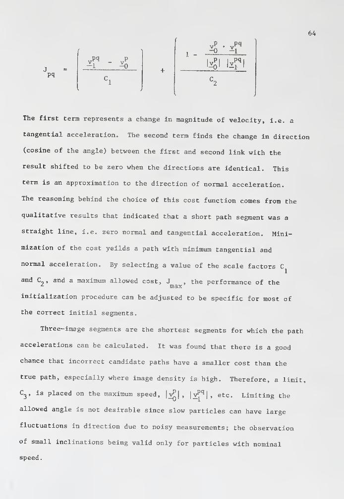
We can then write (while reverting to vector notation for the residuals)
Pr{aj^l5} - Pr{H|aj^} Pr{a^} = Pr{v^^.v^_J cq) ^^{v^^'^^-il^^o} Prtai^
Pr{a2|5} - Pr{E|a2} ^ria^} = PJ^^^sJ^,!.:^.!I ^l > P'^^:^2'^-ll '^O^ P'^t«2^
Pr{a3|H} = PriHla^} Pria^} = PrCv^i^v^.J cq) Pr{v^2'Vil '^q} PrU^}
Pr{a^|5} - Pr{H|a^} Pr{a^} = Pr{Vj^^,Vj^_^| ci) PrtVj^2'^-l ' ""l ^ ^""^^^
To interpret this, the quantities on the left are referred to as the a
posteriori probabilities of the decision state, i.e. the probability of
the decision state given the features. These are only proportional to the
right hand side because Pr (5) has been eliminated from the denominator.
(Recall that this is just a scale factor.) The Pr(ot ) term is the a
priori decision state probability and is conditioned by the likelihood
of the feature given the state, Pr(5|c^ ). Recall that the decision state,
a,, is the vector composed of all link class decisions. Then, for example,—
i
with a^^ = {cq, cq}, we have
PrCHJa^} = Pr{Vj^^,Vj^_^|co} P'^{:^2'^-ll*'0^
since features are assumed independent. The quantity Pr{_v,^ ,j;j.
^|cq} is
the joint probability of candidate residual v,^
and the last residual v, ^
given a class cq (false) link. As another example, consider
Here, Pr{}Vi»v, ,|ci} is the joint probability of the candidate residual
and the last residual given a true link to candidate image C^ . After
making a few observations, a useable relation will result. Terms like
48
Pr{v, ,v, ilcn} = Pr{c Ico} refer to the probability of the feature—kq -Tt-1 "^
Tvector £ = {v, ,v, ,} given a false link condition. It can be reasoned
•^ —kq -Hc-1
that an image with a confusing false link can occur anywhere in the
window with an equally likely chance. Therefore, any one particular
feature vector has a probability of occurrence that is equal to one
divided by the total number of possible feature vectors. (See Chapter V
for a specific example.) Terms such as Pr{^,|ci} are the probability of
a true link to the image ^ with feature vector C • Figure 3-5 shows
1 2an example for the case q = 2. Two candidate images, ^, and ^ are
found in the window around the prediction z,. Candidate residuals are
V and V, „. A past residual of v is assumed to have occurred at—kl —k2 —k-1
time k-1. The sketch shows contours of a possible residual joint prob-
ability Pr{v" >^T,_ikl^ ^ constants L , L-, or L^. If, for example,
V. ^= d, then the joint transition probabilities A. and A- are found, i.e.
^1 =^''^''kl' '^I'^l^
^2 " ^''^\2' '^'''l^
as shown. The joint probability shown is unimodal but, in general, no
constraints are placed on its form so it could be multi-modal. Since the
residual statistics are assumed stationary, it can be expected that this
quantity could be learned from examples of correct image path sequences.
Before discussing the learning aspect further, the a priori probabilities,
Pr{a^} need to be examined in more detail.
The decision state, a^. , was previously classified according to three
hypotheses: the path stops, continues normally, or branches. It can be
49
2. : prediction
1 2Ci^, £. : candidate images
V,,, v.^: candidate residuals
IMAGE PLANE CONFIGURATION
V. Candidate^ Residual
= constant
u
VlLast
Residual
EXAMPLE OF JOINT TRANSITION PROBABILITY
FIGURE 3-5
50
expected that the chances are much greater that the path will continue
normally rather than stop or branch if there are no missing images and
the image density is sufficiently small to limit the number of overlaps.
As shov\?n in Appendix A, the overlap expectation is a function of particleI
.
density and system resolution. The chance that a path stops is negligible
(if not near the edge of a frame) except in the case of data that were
input using the graphics tablet. For tablet data entry images are
easily omitted and will cause the performance to suffer. In essence,
the a priori probabilities define expectations of what the decision
results should be. They weight the calculations of the a posterior prob-
abilities and, hence, directly affect the selected decision state.
The a priori probabilities vary as the number of candidates changes.
When there are no candidate images, q = 0, it is assumed that the pathK.
stops. Therefore, PriHg} = 1.0. For the case of only one candidate,
it is assumed that the path will most likely continue, linking to the
candidate (Pr{Hi } = .99, PrlHg} = .01). For q = or 1, branching can-
not occur so Pr{H2} = 0. Wlien q = 2, branching can occur so Pr{H2}
is just the probability of image overlap calculated in Appendix A. These
probabilities were found to be negligible for the case of two or more
images. Therefore, when q = 2, decision state a, = {ci,ci} is highly
unlikely. (Thus branching is assumed negligible.) If q = 3, one stateK.
is (cicicj} which has a very small likelihood. Other states such as
{cjCjCq} or {ciCpCj} would have the same probability as a = {c^c^}. It
is clear from the analysis presented in Appendix A that the current data
available is a rather sparce situation since the chance of overlap and
51
confusion are so small. This Is good for the PFM because the expected
number of decisions to be made is small and reduce to picking the one
most likely link. It is important to remember that as the density or
lighting situation changes, the probabilities of the hypotheses, Hq, Hj,
and H2, will change. Returning to the example for q = 2. Define
P = Pr{5 Icq}, q = 1, 2, so (3) can be written
Pr{ajH} « (P^) Pr{Ho}
Pr{a^|5} « A,P„ Pr{Hi}-2'--' 10
Prfa^lH} cc p^Aj Pr{Hi}
2
Pr{a^|5} « h^A^ Pr{H2}
where A and A- are the probabilities Pr^Ail'^l^ ^^^ ^''^^L.jl^l^ • Now,
it is assumed that PriHg} and Pr{H2} are very small compared to Pr{Hi}.
Therefore, the decision amounts to a choice between states a^- and ot„.
Bayes minimum error rate decision rule (2) reduces to:
Choose a_ if A^ > A- and ot. otherwise.
When A^ and A„ are very small, the probabilities for a», a^_, and a. are
small allowing the possibility of 01 . Therefore, the decision rule becomes;
Choose a if P Pr{Ho} > Aj^PrCHj} and P^PrfHo) > A2Pr{Hi}
This just says that when neither link has a probability greater than the
chance of a confusing image being present, the path should stop (dacision
state a, ) • Finally, when A^ and A» are both large, state a, becomes
theoretically possible. The decision rule would be
52
choose a, if A,Pr{H9} > P ^"^^"l^—4 1-^0-
2
and
A-Pr{H2} > p Pi^^HlJ
2"
2
This completes the example. A decision can be made as to which is the
most probable state. It is evident that the a priori assumptions are
very important in the stop-path and branch decisions but do not enter
in the normal condition where one link of the candidate links is chosen.
Similar results can be obtained for other values of q .
^kLearning
. An important aspect of the PFM is the determination of the
residual transition probabilities. It has been shown that this reduces
to determining the joint probability of the feature vector given a true
link, Pr{_^|ci}. Used here is a nonparametric procedure of identifying
the feature probabilities. (See Duda and Hart, 1973.) To determine these
feature likelihoods, the PFM is given path examples that have been pre-
viously identified by manual effort, or alternatively, by previous output
(which has been verified by an operator) of the PFM. An identified image
path is a sequence of images that have true links. Therefore, no deci-
sion has to be made, the filter can be given the sequence as input. As
the filter follows this path a residual will be generated
-1' -2' ^3"--'^k-l' ^•
This sequence contains examples of residual transitions for true links.
By using several paths (the training sample), many example transitions
are generated. The residuals are quantified and the transitions v to—k-1
53
V, are counted to form a histogram of transition probability. There
are two histograms that result:
^'^Kq' Vl'^l^ ^°^ ^'^^\q' Vl'^l^-
These are used by the PFM to make decisions on new data as discussed pre-
viously in this section. The decisions made by the PFM are then dependent
on the training sample. As the characteristics of the training sample
change, the PFM's decisions will change and thereby adapt to the char-
acteristics of the flow being studied.
Control of the PFM
With the capability of making a decision as to the link classes, the
PFM can follow image paths. At each step, the decision state probabilities
can be calculated and the decision state with the largest probability is
chosen. The three possible results are simply the state hypotheses as
presented earlier. It is expected that the normal response will most
often be taken (i.e. only one link found; Hi). When Hq is decided, the
path can simply be stopped. When H2 is decided, branches have been identi-
fied. They can be saved for following after the primary path (the path
with largest link probability) has been found. Dealing with branches is
very difficult; many possible combinations of links occur. For example,
if a path branches and then comes back together or, in general, any case
where a path is split, there is a question as to whether this represents
the true case or is a result of confusion. The only real answer to such
a question is to do everything possible to avoid branches. It is worth-
while to introduce the term isolated path. This is a path whose link
54
state decisions were all for the case of q. = 1. That Is, no branch
decisions were necessary; the window around the estimate contained only
one image. This is what would be considered a "nice" path. If the
measurement noise is small enough and the estimator fairly accurate,
these paths are a reality. Data consisting of isolated paths would have
a high confidence level. Any other situations of confusion and overlap
would have a lower confidence level. As particle density is increased,
the possible confidence will decrease and more operator interventions
may be necessary to resolve confusing cases. The limit to the particle
density, then, is where the cases become so obscure that the operator
cannot be confident in his decision. The limit to the abilities of the
PFM to follow paths is clear. When the link state probabilities are
very close to each other (the decision boundaries) , the decision is not
obvious; the PFM is indecisive. However, for reasonable measurement
noise and density, the PFM control decisions are expected to be correct
more often than not. By monitoring the probabilities (likelihoods) of
the decisions made, an operator can be warned of possibly bad decisions
and poor performance.
Measuring Performance
Perhaps the most frustrating aspect of the particle following
problem is the inability to know precisely what images belong to the
same particle. This means that any measure of error or performance of
the PFM is subject to interpretation. Obviously isolated paths can be
quickly identified by a human observer as well as the PFM. But when
confusion occurs, the true image path is only conjecture. Both the
55
human and the PFM must make decisions, and both will make mistakes. The
determination of performance of the PFM becomes a relative comparison,
i.e. does the path found by the PFM agree or disagree with the human's
belief? The human, of course, has the ability of taking more factors
into account than the PFM. However, the PFM is expected to be more con-
sistent in applying its concept of what an image path is. If the PFM is
made more sophisticated, it would be expected that its decisions would
agree to more of an extent with the human. However, there is a trade-off.
If a semi-automatic procedure is used that has a good performance and
only a few links are wrong and need human intervention, it might be best
to avoid making a more costly and complicated PFM. This can only be
judged with a great deal of experience using the program. For the
present, the performance of the PFM is judged against results given by
Jackman. No procedures were developed to handle special cases so the
error rate is not artifically decreased. Nevertheless, the performance
is fairly good as will be shown in Chapter V. When automatic data
acquisition techniques are used and the variance of an image's location
is reduced (probably by an order of magnitude) , it can be expected that
the present PFM will provide satisfactory results. It is conceivable
that when errors are detected, the path in question can be discarded.
Alternatively, it can be kept if the choice is between two images that
would not alter the description of the flow field significantly. The
choice of how to deal with these "differences of opinion" allows the
experimenter to select his experimental accuracy and confidence. It
may be discomforting to know that the performance cannot be stated
56
quantitatively, but at least an acceptable level of confidence is
realizable.
Summary
The PFM has the task of identifying image paths (patterns) in the
data array S... . The approach taken here assumes that an initial path
segment has been identified which the PFM is to extend forward in time.
Referring to Figure 3-5, candidate images, ^, q = 1, 2, ..., q, are
found in a region (the window) around a prediction, z_ , of the location
of the next image of the particle being followed. A decision must be
made as to which candidate image(s) is (are) most likely the correct
image(s). To do this, the probability of the transition v, , to v,—k-1 -^tq
is assumed known. The images with the most likely transition prob-
abilities are selected as true links. If more than one image is selected,
branching occurs. The PFM continues following only one branch, saving
the remaining branches to be followed at a later time. If no images
pass the requirements, or no images are in the window, the path is halted.
The normal situation is for only one image to be selected with index q .
This defines the measurement, z, ^. A Kalman filter is used to generate
the prediction, and its residuals are used as features in the decision
process. The sequence z, ,k=k,k +1, ...,k +n -lis the—k o o o p
identified path, where k is the initial frame of the path and n is theo p
number of frames spanned by the path.
< xT
>-<:
3<x-f
57
i^ - <xt
s^
i
>-
2:oI—*
<_>UJQ
CJ>
3o UJa rvi
2: •—
<
I—i 00
(— LU=3 OO
T-——
—
< nT
*
^>r*
II
UJ o"COO UJO C33: =3:
oU
*h- XX UJUJ o
(_> UJUJ CO—J <tUJ s:00 1—
<
I
L
Jf ''^
I
cr
a.
»o>|#II
cr
+ 1
1
e
00 1—
csz-<3o—J—Iou.
UJ
•—
'
CO
ce UJ<j: cr
UJ •—
I
a: u.
§
oo-JCO
CHAPTER IV
PFM: INITIALIZATION AND IMPLEMENTATION
Presented in this chapter is a discussion of the procedures used
to implement the Particle Following Machine (PFM). The material pre-
sented is not vital to the understanding of results given in Chapter V,
but will aid in the comprehension of where the results came from.
Three logically separate routines are outlined: the initialization
program (INIT) , the Particle Following Program (PFP), and the learn-
ing program (LEARN). Listings of the source codes are given in
Appendix D. Before presenting the details of the programs, it is
necessary to present the background reasoning to the initialization
problem. The PFM, presented in Chapter III, assumes that an initial
segment has been identified and procedes to follow the image path
using its path concept. Finding initial segments must be done with
much less information and is therefore rather difficult. Once the
initialization problem has been presented, the discussion of the
programs is preceded with a short description of the data structures
used by the programs.
Initialization
The Initialization Problem . If the initialization of the particle
paths were simple, the whole problem could be reduced to a series of
initialization steps. However, the problem of finding initial path
sequences is not simple. Required here is a scheme that can take an
arbitrary image location and find its closest successors or predecessors
58
59
representing the path. This must be done without any knowledge of the
path's attributes. Especially important and lacking is any information
concerning the particle's velocity (speed and direction). The data
contains particles traveling at different speeds and many different
directions. The fact that there is a strong general velocity In the
X direction is useful, but as the turbulence increases, it becomes
less dominant. Difficult cases to consider here are the possible
backward motion of a slow particle due to measurement error and the
possible close proximity of a slow and fast particle. In the latter
case, the slow particle has a much higher spatial sampling frequency
that may possibly obscure the faster path whose spatial frequency is
much lower.
Considering this problem in terms of spatial sampling gives some
insight to the difficulties involved. The particles have different
velocities so when sampled at a constant time rate will travel different
directions and distances. Since, in the initialization problem, there is
no information available concerning the particle velocity, the problem
becomes one of identifying the spatial sampling rate of paths of arbi-
trary shape. To make matters much worse, large measurement noise
exists in data currently available making the spatial sampling rate
highly variable. If this were not the case, Fourier transform tech-
niques could be utilized to advantage. Here, spatial transforms of
the data would indicate strong sampling frequencies and directions which
could be identified through filtering. The fact that paths are not
straight causes some problems, but as discussed earlier, the paths
are roughly straight over five time samples allowing one to look for
60
straight line segments. With such a small number of points in the
assumed line, however, measurement error obscures any trend in
the spatial frequency.
The beauty of using spatial transforms is that they utilize all
possible information available in the initialization step. This in-
formation consists of knowing that in any region of the data array S,
there are straight lines that have different directions and different
spatial sampling rates. Therefore, the result of the initialization
step should be groupings of the images by path segments. The number of
groups are unknown, but each group contains up to a certain number of
images (the number of time samples considered in the region) whose
time indices are monotonically increasing. The reason for the unknown
number of groups is that the spatial dimension of the region under
consideration is arbitrary and hence may sever image paths leaving
a segment not starting at the time boundary of the region. This view
of the problem is that of a constrained clustering problem which could
also apply to particle following. The difference is that the particle
follower makes use of path history. Therefore, initialization is a
special case of the particle follower. That is, the probability of
an image in the next time sample connecting to one in the current
time is uniform; all images have equal chance. This is in essence
Jackman's initialization assumption. He then used a constant velocity
criterion to locate the next image. If only one image was located,
he assumed he had found the start of a path, otherwise he arbitrarily
chose one. This approach also returns to the problem of considering
all image path possibilities. As the image density increases, the
61
number of possible paths increases and the possibility of confusion
increases, thus making this approach far less desirable.
An Initialization Procedure . The final form of the initialization
program is an implementation of heuristic search procedures. A
particle in the first frame to be analyzed is chosen as the base or
reference. A window is constructed around this location with a size
sufficient to contain the next four images of the particle represented
by the reference image. All possible three-image paths are then found
and a cost calculated for each. The path with the smallest cost is
possibly a valid path. If other paths have costs within 10% of the
minimum cost, they are retained for further processing. Three- image
paths are not typically adequate for initial path segment identification;
there is too high a chance that three arbitrary images will have an
accidentally low cost. Therefore, a fourth and fifth frame of data
is considered. A new candidate path is formed by connecting each of
the low-cost paths identified in frames one through three to each image
in the window at frame four. The last three images of each candidate
are used to calculate a three-image path cost as previously described.
The cost from the first three and the last three images are summed
to make a cost for the four-image paths. Those paths with costs within
5% of the minimum are considered likely initial segments. Now, frame
five images are linked to the candidates. Again, the last three
images are used to calculate a cost which is added to the total cost
of the path calculated up to frame four. Finally, those paths having
costs within 3.3% of the minimum are selected as initial path segments
to be used as Input to the particle following program. The criteria
62
for closeness changes from 10% to 3.3% because the costs are being
added. This causes the total cost to Increase, so, by decreasing the
percentage, the criteria remains roughly the same. Note that this
technique does not guarantee that the paths found are the overall min-
imum cost paths because only three Images are used at a time. This
was done in lieu of using all possible five-image paths which would
be very time consuming and expensive.
To be more specific, we define the reference image position
(in frame k.)asr = (i,j). A region surrounding this point in
space and time (called a window) is defined as
Window Rw
1 ^ 1 < 1w wmin max
J ^ J ^ Jw wmin max
k < k < k +4o o
The size of the window is selected to include five samples of the
fastest particle. The qualitative observations discussed in Chapter II
indicate that images typically travel in the +u direction with small
inclinations to the v = axis. Allowing for the possibility of a
noisy, slow particle backing up, i is selected slightly less thanmin
i . Then i is set at roughly six times the maximum expectedmax
velocity. Finally, j and j are set to allow the fastest imagemax rain
to be inclined approximately twenty-five degrees up or down. With
the window boundaries fixed, the image data set can be searched
for all images within the window. The resulting list of images is
63
defined as the candidate image list. Assuming that there is a true
path segment among all possible paths that can be constructed from
the candidates, one approach would be to calculate the cost of each
path as a function of its five images. Then the minimum cost path
would be the path most likely to be the true path. In order to save
computation time, a slightly modified procedure is used.
A cost function is defined for any three-image path. This cost
function is a heuristic whose specification was guided by qualitative
observations as well as trial and error. Basically, the cost is designed
to be minimal for a straight, evenly sampled path with a spatial sampling
rate (absolute speed) that is reasonable.
Consider a window containing n images in frame k + 1, n„1 o 2
images in frame k +2, etc. Then, n, links connect the referenceo 1
image at r^ to _r. (images p in frame k + l,p = 1,2, . . . ,n|^) .
qEach of these links could connect to any of the n2 images x_2
in the third frame (time k + 2) making the total number of possible
three-image paths, n. x n„ . For each two-image link, a first dif-
ference is defined as
k to k + 1 : v^ = r? - 1^ Vo o — —1 — p
k + 1 to k +2: v^*^ = r^ - r^ Vo o —1—2 —1 pq
The first difference is a vector quantity that is a first approximation
to velocity. The cost function, J is then defined for each two-linkpq
(three- image) path segment using the reference image, image p and image q.
The form for the cost is
65
Extending the search to five images reduces the number of errors
even further. To accomplish this, the search procedure looks for low-
cost paths in the first three frames. Then, using frame four (k +3),
each of the path segments in the reduced candidate list, is extended
to all images r^, r = l,2,...,n^, and the first difference is found
from
^32 q,r
Then, the cost of the last three-image segments is calculated by
pqr
.qr .pq1 -
-1 -2
-pq .qr
where p and q are the image indices for the candidate paths and r is
the index for images in frame four. The cost, J , is added to thepqr
candidate costs, Jp^ , and the low cost paths are determined by finding
those paths whose costs are within 5% of the minimum. This procedure
is then repeated using the images r^, s = 1,2 n in frame five.
Here, the first difference is
rs s r^3 =^4-^3 r,s
and the cost becomes
qrs
I
rs- Iv^l
1 -
,rq'^ rsV • V-2 -3
where q and r are indices of images in the candidate paths and s is
the index of images in frame five. This cost is added to the candidate
costs to give a total five- image path cost for a given candidate path:
66
J = J + J + Jtot pq pqr qrs
Those paths whose overall cost is within 3.3% of the minlmun cost are
the final initial path segments and are used as input to the particle
following program. Chapter V shows the results of using this initial-
ization procedure and discusses some of the special problems encountered.
The Data
Since this work focused on the theory of particle following,
new experimental data was not taken from the flow apparatus. Instead,
the data analyzed by Jackman (1976) was utilized. This consisted of
55 frames of raw image locations as generated by manual entry via
the data tablet as well as the manually identified invertible paths.
This data was collected using the small prism for a flow with Re = 3500
at 20°C. A film rate of 25.7 frames per second was used to expose
Tri-X film through a 100mm lens fitted with a close-up attachment.
Images by Frame . Data, as entered via the tablet, consists of the
image locations in the film plane (i, j, k) . At these locations,
array S, (see Chapter II), has the value '1'. The image locations
were entered systematically, but not necessarily in any sorted order.
Therefore, this data was sorted by i value which allows somewhat faster
windowing. Each frame of data contains different numbers of images
which, for the present purposes, are best stored as a vector of all
images and addressed via an index to the first image of each frame.
Three vectors are then used to represent the frame-by-frame data:
NPART, KINDEX and DATA. (See Figure 4-1.) NPART and KINDEX must have
dimension at least as large as the number of frames needed. (Not all
67
^1 -^a ^2 h
KINDEX
Frame 1
Pointer
Frame 2
Pointer
Frame 3
Pointer
lwNVVV\V^
DATA
NDATA
# of imagesin Frame 1
# of imagesin Frame 2
FRAME- BY- FRAME DATA
FIGURE 4-1
# of imagesin Frame 3
ID START FRAME LENGTH
1l Ji ^o Jo T-j J1 ^1 '2 ^2 '3 ^3 •
•
IMAGE LIST
ID START FRAME LENGTH
\ Jj ^2 ^z ^3 ^^3
IMAGE LIST
INVERTIBLE PATH DATA
FIGURE 4-2
«yVAr^
68
frames are necessarily used.) DATA has dimension at least as large
as two times the number of images since each image location has an i
and j value. The numbers obtained from the tablet were integers but
when used by these programs, they were stored as real numbers. This
allows addressing of the data as a complex array equivalenced to the
array DATA. Then, when convenient, both i and j values of an image
may be retrieved by only one index. The frame-by-frame data were
rotated and translated to common axes and, without loss of generality,
the origin was set at the lower right hand corner of the tablet as
opposed to the image plane coordinates used in Chapter III. This
merely shifts the j values making them always positive. The portion
of this data set used by any program is currently stored in core which
simplifies the programming and speeds up execution.
Invertible Path Data. The second major data set consists of the in-
vertible paths identified by Jackman. These are the path sequences
Pp. Each sequence has a length, a start frame number and the image
locations. This data set is accessed sequentially, path by path and
is not saved in core. Its structure is shown in Figure 4-2. The
paths are not in any particular order, but each path has an identifier,
ID, that was assigned by Jackman. Conjugate paths were the only
paths put in the data set, but they were not necessarily located
next to each other. When comparing the output of the PFM to the
paths in this data set, it was necessary to build an index that located
a path by its first point. However, because this data was manually
identified and punched, many errors occurred (they were typically small
since gross errors were corrected) making it impossible to compare
69
the results automatically. In addition, the paths in this data set
include generated points that were used to fill in missing data points.
The PFP was not built to handle this case since new automatic data
entry procedures will not have this problem (Llndgren, 1977).
The Initialization Program
The FORTRAN program written to perform the initialization procedure
is outlined in Figure 4-3. The main program, INIT, primarily handles
the selection of a reference image, various counters, and outputting
of the results. Subroutine REDDAT establishes the data arrays contain-
ing the image locations, frame start pointers and frame lengths as
discussed previously. Options allow the selection of printing inter-
mediate steps, plotting the results and storing or recalling the data
in the directly usable form generated by REDDAT. Input data to INIT
also includes selection of the time and space window boundaries. Sub-
routine WINDOW searches the data for images in a specified window.
Data is required to have been sorted by i values which speeds up the
search significantly. Subroutine TRAK determines the minimum cost
paths. The FORTRAN source code is listed in Appendix D and contains
additional documentation of these routines.
The Particle Following Program
The implementation of the particle following machine is the
Particle Following Program (PFP). This routine takes the initial path
segments identified by routine INIT and attempts to follow them for
a specified number of frames. A simplified flow chart for the PFP
is given in Figure 4-4.
READ OPTIONS, INPUT DATA
READ IMAGE DATAFOR FRAMES ONE TO NTS
PLOT IMAGE DATA FORFRAMES N SO - NTS
SELECT A REFERENCE IMAGE
FIND ALL IMAGES IN WINDOWBASED ON REFERENCE
FIND MINIMUM PATH(S)FOR REFERENCE
NO
YES
WRITE RESULTS
PLOT PATH SEGMENTS
END
70
SUBROUTINES
(REDDAT)
(WINDOW)
(TRAK)
SIMPLIFIED FLOWCHART OF"INIT"
FIGURE 4-3
71
I READ OPTIONS
READ IMAGE DATAI
READ PROBABILITY MATRICES!
READ INITIAL SEGMENT |
I INITIALIZE FILTER |
UPDATE INITIAL VALUESSAVE DESIR
"^ WINDOW
D RESULTS
ESTIMATE
DECIDE WHICH IMAGETO USE
SAVE RESULTS
UPDATE ESTIMATEUSING NEW MEASUREMENT
SUBROUTINES
(PFPRD)
(LRNMAT)
(FILTER)
(UPDTE)
(WEST)
(DECIDE)
(UPDTE)
END
SIMPLIFIED FLOWCHART OF "PFP'
FIGURE 4-4
72
This program begins by reading the options which consist of
writing or recalling the image data in a directly useable form (as
in INIT), and writing intermediate results. Subroutine PFPRD is
functionally identical to Subroutine REDDAT used by INIT. However,
larger data arrays are specified since PFP needs at least as many
frames of data as images in the desired path. LRNMAT reads the joint
probability matrices used in the decision process. These matrices
are the output of the program LEARN which is discussed in the next
section.
After the preliminaries, an initial segment is read. This con-
sists of five sequential image locations assumed to start in frame
one. (Only paths starting in frame one were considered for the demon-
stration of the particle follower.) The path state is then initialized.
The location of the first image is assumed to be the path's estimated
location. The initial velocity is calculated from the first difference
of the first two images in the initial segment, and the acceleration is
assumed to be zero. These values specify the initial state ^ (-)
•
The initial covariance matrix is specified as
P (-) =
r 10
10
which reflects fairly large uncertainty in the initial position, less
for the initial velocity and even less for the initial acceleration.
Initialization of the filter in this manner forces the first two images
73
to be used and their resulting error to be zero. Other possibilities
exist such as forcing all five images in the initial segment to be
used and calculating an approximate initial state from them. By
utilizing only the first two images, some errors in the initial paths
can be eliminated, and some incorrect initial paths can be eliminated
entirely. (Recall that the initial paths are not guaranteed to be
correct.)
Once the initial estimates are fixed, the Kalman filter sub-
routine FILTER is initialized. This is a multiple entry routine which,
on initial call, sets the $, H, and R matrices used in the Kalman
filter equations. Entry UPDTE, calculates a new estimate using the
latest measurement, and entry EST, calculates the predicted state
(the estimated state prior to a measurement). Once the updated initial
state has been determined, PFP enters a loop that attempts to follow
the path as far as possible.
The following loop consists of making a prediction by calling EST,
windowing the estimate with WEST, choosing the next image with DECIDE,
and finally, updating the state estimate using the new image (measurement)
with UPDTE. Windowing the PFP is two-dimensional since only the images
surrounding the prediction, at the same time, are required. The actual
search for candidate images is the same as for subroutine WINDOW used by
INIT. Subroutine DECIDE, calculates the candidate residuals, and using
the joint probability matrices, selects the candidate image that would
produce the most probable error. A check is made to determine whether
the decision is isolated and a message is printed if it is not. In
addition, a simple check is performed to determine whether the
74
choice made was different from the minimum error choice (choosing the
image closest to the predicted location). If it was different, another
message is printed. Finally, if the probability of the chosen image
is less than the minimum allowed, DECIDE sets a flag to stop the PFP
from following the path further. After a candidate image has been
chosen for use as the next measurement, the UPDTE entry to the filter
routine is called to update the state estimate. The following-loop
continues until the path is stopped by subroutine DECIDE, or the speci-
fied number of images have been identified for the path. The results
are then printed and the next initial segment is used. After all
initial segments have been followed, PFP is finished. The PFP source
is given in Appendix D with additional documentation.
Program LEARN: Determination of the Joint Probabilities
Routine LEARN is very similar to PFP. it takes a given path
(identified by earlier manual effort) , and applies the Kalman filter.
The transitions of the residuals are quantified and counted, thereby
developing histograms of the joint probability to be used in PFP. A
simplified flow chart is given in Figure 4-5.
A path is read by the program and initial state estimates are
made in precisely the same manner as in PFP. The same rountine FILTER
is used to propagate the state estimate over time. After the path has
been "followed" (the measurements in this case are known beforehand),
the residuals are added into the probability histograms by routine SAVE.
After all the paths to be analyzed have been studied, the resulting
joint probability matrices are output. The source and additional
documentation for LEARN is given in Appendix D.
75
READ A path"]
INITIALIZE STATE ESTIMATE
INITIALIZE FILTER
UPDATE ESTIMATEWITH FIRST MEASUREMENT
CALCULATE PREDICTIONSAVE RESULTS
UPDATE PREDICTIONWITH NEW MEASUREMENT
YES
ENTER RESULTS INTO
PROBABILITY MATRICES
YES
WRITE RESULTS
END
SIMPLIFIED FLOWCHART OF "LEARN"
FIGURE 4-5
SUBROUTINE
(FILTER)
(UPDTE)
(EST)
(UPDTE)
(SAVE)
CHAPTER V
RESULTS OF PERFORMANCE TESTS
Initialization
Program INIT was used to find initial path segments composed of
five images with the first image in frame one. The data used was col-
lected by Jackman (1976). Identification of Initial path segments
is dependent on the values of parameters Cj^, C2 and C3 used to calculate
the cost of three-image segments. To observe how these parameters af-
fect the cost, consider a three-image segment (ij, jj), (±2, J2)» and
(io» Jq)- Define vector A as a vector from image one to two, and
vector B^ as a vector from image two to three. Then the cost function
may be written as
"^total - ^T"•
"^N
where
JN
B|
77
COST
"0.50 0.25 0.0 0.25 .0.50
iBJv-- IrtI iUNITS PER SWMPL£)xlO* 2
J-j-: COST OF TANGENTIAL ACCELERATION
t^NGLE COST
78A • B
(= cosine of the angle between A and B) for various values of|A| 111
C and C . As the parameters C and C increase, the cost of a specific
difference in speed or angle decreases.
This, in effect, decreases the cost of the vector velocity varia-
tion between A and B^. For the results given here, the parameter values
found to give best performance were as follows:
C = 40.
C = 1.0
C = 30.0
Recall that the last parameter, C , is a hard upper limit on A and B^-
The upper limit on cost, J , was arbitrarily set to one. Therefore,max
many combinations of J and J exist that produce costs less than J'T N max
Figure 5-2 shows the contours of J . The contour, J , = 1.0,^ total total
is the limit, so any point within this contour would represent an
allowed three-image segment.
Figures 5-3 and 5-4 show the initial path segments as found by
INIT. The locations of the symbols '1' through '5' represent locations
of images in frame one to five. (This figure is just the superposition
of the first five frames of data.) A proper path segment consists of
five sequentially numbered images. Figxire 5-3 shows data from the
"top" section of the frames, i.e. one stereo view. Table 5"! describes
labeled segments in these two figures. Important to note here, is that
the output of INIT contains several different kinds of errors. Most
errors are a result of data entry from the tablet. When using the
tablet for data entry, numerous images were accidentally omitted or
79
liTi «\'
7/ /'
/ / ,/-
; / /.1 I
I, \
\ \ VI, I \
\ \
\ o o o
\
\ \ \ -*
\ \ \ " "
\ \ \ cT J"
oCO
\
\ 1 1
ai'jNd Ni 3aioy3JdiQ•o ero- i!S"t
ijr • T _
83
entered twice. In addition, a failure of the tablet to correctly
locate an image could occur because of operator error. This caused
some image locations to be displaced to the left as seen in Figures
5-3 and 5-4. These errors are not considered in the overall perform-
ance because they are expected to have been eliminated by technique
modifications as discussed previously. The significant errors in
these results occur when the image density is high and incorrect initial
paths are selected. Some of the errors can be corrected by the particle
following program (see last section. Performance of the PFP). Another
error is not starting a path for an image in frame one. This usually
results from the cost of the path being too high and can be corrected
by increasing J . However, this must be done carefully because many
erroneous paths may also be allowed. The parameter values chosen re-
present a trade-off in this regard. Very few "good" images in frame
one were lost.
Performance of INIT . Table 5-2 contains the results of initialization
of frame-one images. The different types of errors that occur are
categorized by whether or not an image in frame one was "startedi"
i.e. an initial segment was found starting with a frame-one image.
An initial segment can have one or more incorrect members, be in
error because of a double entry of the image's location, or be the
result of an inadvertently added frame-one image. If an initial
path is not found for an image, there are a number of possible reasons.
The cost of a correct path may be too large, images may be missing or
inadvertently added, the tablet could have caused a displacement of an
image, or the correct path does not have five images in the field of view.
84
Except for the first of these errors, too high a cost, these errors
are a result of using the data tablet and are unavoidable. Of the
254 images in frame one, 47 were classified as images with unavoidable
data entry errors and were disregarded. Of the remaining 207 images,
148 were started correctly, 31 were started with at least the first
two images correct, 11 were started incorrectly (totally wrong) and
15 were not started because their cost was too high. These results
are expressed as percentages in Table 5-2. Note that initial segments
with the first two images correct are sufficient to start the PFP and
may possibly be correctable. Initial segments that are totally wrong
may be followed by the PFP but would be expected to be aborted as
short (up to five-image) paths since the chance of these inadvertent
paths being longer is very small.
TABLE 5-2
INITIALIZATION PERFORMANCE ON 207 FRAME-ONE II^GES
IMAGES STARTED
CORRECT FIVE-IMAGESEQUENCES
INCORRECT BUT WITHTHE FIRST TWO IMAGESCORRECT
TOTALLY WRONG
72%
15%
5%
CORRECT OR87% CORRECTABLE
IMAGES NOT STARTED
COST TOO HIGH 8%
85
Particle Following
Learning Results . Program LEARN generated the joint probabilities
as described in Chapter III from a training sample of fifty arbi-
trarily selected image paths that had been identified by Jackman. The
resulting probability distributions are dependent on the finite fading
memory parameters. Figures 5-5 through 5-3 show the distributions for
s = 1.0, 1.2, 1.5, and 2.0. Using other arbitrary groups of fifty
paths gives reasonably similar results. These graphs are interpreted
in the same manner as the example discussed in Chapter III. In general,
these results are fairly similar for the different values of s. As s
is increased, there is a slight change in Pr {v |Vi^_i} to change from
rV
IV
positively correlated to negatively correlated. The Priv |Vi^_il also
becomes negatively correlated. Some distributions are seen to be
multi-modal, but only slightly. All of the distributions have non-
zero means and show some dependence (correlation) . Checks were made
of the cross-correlations between u and v residuals and no significant
dependence was found. Furthermore, correlations were not found to be
significant between v, and v , v etc. Therefore, the assumptions~^^
~k-2 ~k-3
made in Chapter III about the residual appear reasonable.
The probabilities for the u and v transitions are seen to be dif-
ferent in character. One possible explanation for this comes from
considering the odd image shapes. Analysis of the tablet error in
Appendix C assumed images to be circular. As shown in Appendix A,
particle movement causes the images to be lengthened in the u direction.
Therefore, the variance of the u location of an image should be larger
than for the v location. This effect shows itself in the u residual
c:j
°i
oj
II
UJ
oo
00I
ooII
o
oo
00 •
86
yr\ rH
:,.m\\\\ v: III! i
I
On ''3-
1.1;
1 \- '^
I r 1
CL
Ij IJ iJIJ'
ou IJi
iunnr:,ji:j A ix:jn
II
CQcCCOoCl.
(T)
LOI
LO
CD
i I / / /"i^ \',;•
:• ,
I
I
'1. ^-.
I ',
,/
N
89
ooII
on
oo
IJG 1
II
h-zLU
5I
^ I
g I
o
OU IJ
I
/XL
-, o cr
:.i .;.///:r:^rCKsN\.\\,,,
/ / /
v^
X J
00 "LV fji.rn 1.10'
4
iHrii:i[s:ju a ixgi
Li-I
c.;i
oirrii
\ o
\\.
\ V
no '[n
oCVJ
II
1/1
CD
90
probability contours. There is seen to be more variance in the u
residual transitions than for the v residuals. This effect does reduce
the performance of the PFP. With an improved experimental technique
(Lindgren, 1977), in particular the use of a strobe lighting system,
the images will be more symmetric. The reduction of performance due
to this is discussed further in the last section of this chapter:
Performance of the PFP.
Performance of the PFP
The PFP was used to identify paths whose initial segments were
those determined by INIT (see Figures 5-3 and 5-4). The resulting
image paths were verified manually using the raw image data. Various
classifications of an identified image path can be made. A path can
be completely correct, starting with an image in frame one and contin-
uing until the image is out of the field of view. Alternatively, a
path can be correct but short, i.e. not include all images before the
image goes out of range. One reason for a path being short is that an
image is missing having been inadvertently omitted during data entry.
Various other reasons will also cause the path to be short. These
include exceptionally large errors in image location or unexpected
particle motion. It was found that short paths typically were dis-
continued because there were no images in the window, or the probabil-
ity of the link decision was too small, i.e. less than the probability
of the stop-path hypothesis. Short, correct paths, then, are not
extremely important errors since the data entry procedure can be
improved. Of more importance are the "jump" type paths. These paths
91
start correctly, but when confusion occurs, the Image path selected
shifts to another particle's image path. This error is very difficult
to detect since it originates from confusion. It is expected that
the experimenter would have to make the final decision on whether or
not an image path has jumped particles.
Finally, as discussed previously, the initialization procedure
does not guarantee correct initial path segments. These errors may
be classified by the number of incorrect images that the initial path
contains. The PFP uses only the first two images to initialize the
image state, the other three being useful only to help identify cor-
rect first and second images. Because of this, the PFP has the capa-
bility of finding the "correct" path even if errors exist in the initial
segment. The type of error that cannot typically be corrected occurs
when the first and/or second image is in error. For this case, the
initialization of the image state is incorrect. Initial paths with
this type of error tend to "cut-across" other correct paths. This
is only an accidental situation and it is found that if these erroneous
paths are followed, they are very short, (less than five images long).
Serious errors occur if the initial image is wrong and is linked to
another particle's image path, i.e. another type of jump situation.
This occurs mainly when the correct image path could not be started,
e.g. due to tablet error. The PFP was found to follow very few of
these paths. Table S-'S details the actual occurrence of these errors
for the data studied. It can be seen that over 80% are correct but
not necessarily full length. Only 6% of the paths had severe errors
where the path jumped to another particle's image path. The remaining
TABLE 5-3
PFP PERFORMANCE, s = 2.0
92
Completely Correct
Partially Correct, short
Image Missing
Other
Incorrect, short
Bad Initial Paths
Length < 4
4 < Length < 7
Length > 7
Duplicate Paths
33%
12%
37%
5%
11%
<1%
<1%
1%
82%
93
bad starts were all short and thus easily identifiable. The duplicate
paths resulted from one instance of a double entry for a frame-one
image and another where two initial paths were the same except for
the fifth image. (Recall that INIT will output initial paths that
have very nearly the same cost as was the case here.) Of the initial
paths that were considered "correctable" (first two images correct),
95% were in fact corrected while 5% (one occurrence) were not corrected.
The results also allowed the accuracy of the decision process to
be examined. There were 2363 decision states determined. These are
broken down by the number of images in the window as follows:
^y^ occurrence percentage
48 2
1 1054 44
2 848 36
3 295 13
4 101 4
5 17 1
There were no occurrences for q > 5. As can be seen, a large number of
decisions made were for the case q = 1 supporting the observation that
the data is fairly sparse. Of the decisions for q > 2 only 62 (5%)
were made counter to the minimum distance choice (choosing the closest
image to the prediction). Of importance here, is the fact that 80%
of these decisions were correct. Therefore, the decision rule used
was helpful in finding the correct decision state.
94
Finally, the isolation of the decisions was measured. Isolation
refers to the separation of the selected link probability from other
candidate links. When the probabilities are close, there may be less
confidence in the decision. Table 5'^ shows the distribution of
isolation. It is evident that most decisions were isolated by at
least 10%; 89% by at least an order of magnitude. In fact, of the
cases where the decision probabilities were within 10% of each other,
no mistakes were made. This does not mean that isolation of the
decision did not indicate where errors occurred, i.e. jumps. However,
these occurrences were rare.
TABLE 5-4
ISOLATION OF DECISIONS
Pr{ links not chosen)Pr{ chosen link}
1.0 > 1% ^ 0.9
0.9 >10% > 0.1
0.1 > 9% > 0.01
0.01 >80% > 0.0
CHAPTER VI
DISCUSSION AND CONCLUSIONS
It is evident from this work that following trace particles in a
turbulent flow is not a straightforward data acquisition and reduction
problem. Two major areas were studied: the system optical character-
istics and the procedures used to follow particle images from frame
to frame.
The optical system generates stereo views of the trace particles
and records their images on film. It was found that the pipe and prism
have an astigmatism that alters the shape of the image and moves the
true image location away from the image's center. Perspective causes
parallel vertical lines in the pipe to be nonparallel in the film
plane, and is the reason that a meridional ray analysis is only approx-
imate. These errors become important as the system's resolution improves.
The optimal data acquisition system would be one that produces very small
particle images with minimal perspective error. In practice, this is
not attainable and some measurement error will always exist. Small
image size is also necessary to reduce the probability of overlap in
the image plane. Confusion was presented as the probability that two
or more images occur in a small region in the film plane. This was cal-
culated from the ray trace results and found to be very dependent on
the particle density and lighting situation. Current experimental data
was seen to be fairly sparse with a small probability for confusion and
negligible chance of overlap.
95
96
A theoretical basis was developed for a particle following machine
using statistical decision theory and pattern recognition techniques.
A feature vector was made from the residual of a Kalman filter with
finite fading memory. It was modeled using learned residual tran-
sition probabilities of previously identified image paths. This, to-
gether with the confusion and overlap probabilities supplied sufficient
information for the use of a minimum error rate Bayes decision rule.
The particle following machine was demonstrated with a FORTRAN
implementation using previously collected data. It was found that the
performance was reduced primarily because of data tablet errors. Other
errors were due to confusion and are expected to occur for any data
entry procedure since they are directly dependent on particle density.
Therefore, to maintain the same level of performance with a higher
particle density, the region of the pipe that is Illuminated would have
to be reduced. The demonstration considered only the forward following
problem. A data reduction and analysis system for extensive production
use could apply these concepts as a core and have auxiliary programs
that handle data management economically. This would naturally lead to
a sophisticated semiautomatic procedure where the data can be verified
or corrected as necessary by an operator who can make decisions beyond
the capability of the particle follower. Until a better dynamic model
is developed for particle motion in turbulence, a fully automatic pro-
cedure is considered to be undesirable. Furthermore, the particle
following machine is designed to be adaptive and improve its performance.
This is accomplished by learning residual transition probabilities for
different flow situations. A lack of available data prevented a
97
demonstration of this. However, performance can be expected to be
good as long as the assumptions about the image motion remain valid.
These assumptions are quite general and basically require only that
the sample rate be adequate to allow paths to be approximated by straight
line segments over five samples.
Finally, an initialization procedure was developed using a heuristic
cost function. It was shown to have few severe errors because many
errors were correctable by the particle follower.
In conclusion, the machine learning approach to following trace
particles appears to be a viable technique that can perform at an
adequate confidence level.
APPENDIX A
ANALYSIS OF THE DATA ACQUISITION SYSTEM
The Data Acquisition System
Figure A-1 shows the (y,z) plane section of the pipe and prism
and defines coordinates used in the following description of the sys-
tem configuration. The right-handed coordinate system (x,y,z) is
centered in the pipe with x in the axial direction and z the vertical
axis. The pipe's centerline is aligned with the x axis; inside and
outside diameters of the pipe are R. and R„ respectively.
The Prism
The prism, used to generate two stereo views of the particles,
is mounted on the side of the pipe at the observation station with
its principal plane in the x = plane. Castor oil fills the region
between the pipe outer wall and the prism to match the refractive
properties of the pipe and prism. The refractive index of the plexi-
glass pipe is approximately 1.49 and that of the prism is 1.52.
Castor oil's refractive index of 1.477 is close enough that here,
the pipe and prism are considered as having only two refractive
surfaces; the pipe's inner wall and the prism surface closest
to the camera. For this description, the prism mounting is assumed
true, i.e. no misalignment. Therefore, the prism apex angle of 2Q
is bisected by the y axis at point C which is a distance h from the
origin. The prism has length L and height d (line CD). There are
only two pairs of refracting surfaces of interest in the configuration,
98
100
Surfaces with sides (AB, AC) form one effective prism with apex
angle ^ at A. This top section produces one stereo image which
ideally fills the upper half of the front image plane (see next
section). The second prism is formed by sides (AB, BC) and causes
the second view of the particles to be generated on the bottom half
of the front image plane. Even if there is camera misalignment
(a,3,Y,X^,Z^ ^ 0), the top and bottom images will be separated by
the image of the prism edge C.
Two small light sources are mounted on edge C to provide ref-
erence points on the film records. The particle image locations are
measured with respect to the reference points. This is adequate
unless the pan and tilt of the camera are significant. In the course
of the work, the error in using just two reference points was found
to be significant especially in the rotation correction. It should
be clear that any error in digitizing the reference point locations
(and there is some) will cause errors in all image locations in
that frame. The solution, of course, is to use enough reference
points to allow accurate empirical determination of the camera
location and direction. Duda and Hart (1973) present such a tech-
nique. It utilizes reference points of known locations to completely
determine the camera parameters. This is being incorporated in
future work (Lindgren, 1977).
The Camera
The camera is located by the position of the center of its
aperture (X^.Y^,Z^) and the direction of its optical axis specified
by the pan angle a and the tilt angle 3. (The camera could be located
101
by a point on its stand by using a second transformation of coordin-
ates.) The front image plane is a convenient way of representing the
image (film) plane. It is perpendicular to the optical axis at a
distance F' from the aperture (F' is the back, focal length BEL) and
rotated by an angle y about it. Images in the front image plane
are not inverted as in the film plane. If the camera is aligned
carefully for an experiment, a,6,Y,X , and Z will all be very small
and can be neglected. To use the assumption, as did Jackman, that
rays of light to the camera are parallel, the camera distance from
the pipe Y must be large. This, of course, requires camera lensesA
of long focal length whose field of view will cause the prism to
fill as much of a frame as possible. But long focal length lenses
typically do not focus at nearby objects, so a close-up lens or
extension tube is required. Extension tubes are preferred over
close-up lenses because they cause less degradation of the depth of
field than close-up lenses. However, close-up lenses are typically
corrected to give a flat image plane which is needed in precision
work. The trade-offs in the camera system have only been qualitatively
considered. The current camera system design being used is a result
of trial and error. Analyses of the pipe and prism optics performed
in this work are made using the assumption of a perfect camera since
it is assumed to have better optical quality than the pipe.
Effects of Particle Motion During Sampling
The camera also performs the time sampling function of the data
acquisition system, putting one sample on each frame of film. The
shutter is set to expose each frame for exactly one half the film
102
rate expressed in seconds per frame. (A film rate of 30 frames per
second has a shutter speed of 1/60 second.) The particle will move
during the exposure time an amount directly proportional to its
speed. To determine an approximate magnitude of this motion, con-
sider its average axial velocity,* n, as determined from the definition
of the Reynolds number,
TT D V ReRe = -^ or . TI = -5—
where D is the pipe diameter and v, the kinematic viscosity. Table A-la
shows the distance a particle would move in the shutter time assuming
it was traveling axially at constant velocity as a function of film
rate. It can be seen that for Re = 4000, and a film rate of 30, the
movement would be on the order of %mm. If a fully developed turbulent
flow is assumed, the maximum, u^^^, can be found by using the relation
(Schlichting, 1968, pp. 563-564)
u 2n2
(" + 1) (2n + 1)
where n has been experimentally determined. Table A- lb was generated
using n = 6 for Re = 4000, u = u/0.791. For this Reynolds number
and a film rate of 30, the motion increases approximately 30%, Of
course, these are average values so higher and lower actual velocities
are to be expected. As a particle approaches the wall, typically lower
In this section, u is a velocity component to be consistent withnotation in fluid turbulence.
TABLE A- la
APPROXIMATE PARTICLE MOVEMENT (MM) IN SHUTTER TIME(PJE = 4000)
103
RE UBARFILM RATE (FRAMES PER SEC)10 20 30 40 50
2000
104
velocities are encountered and a particle stuck on the wall will
have zero velocity. These results indicate particle motion is sig-
nificant so actually observed image streaking can be partially
explained when using a constant intensity light source. A fast
strobe synchronized to the camera shutter would eliminate this unde-
sirable characteristic. Planned future work has a strobe system
implemented (Lindgren, 1977)
Approximate Geometric Ray Trace
Optical systems have the interesting property of not being invertible.
That is, the source of a light ray that caused an image point cannot be
located by simply tracing a light ray from the image point back through
the optical system; the source could be located at any point on the ray.
To determine the position of a source, at least two rays are needed.
Each particle forms two images allowing its location to be determined
from the intersection of principal rays traced from the image positions
back through the optical system. Geometric ray tracing is used to
determine the system's projection transform. The actual three-dimensional
ray trace equations would be extremely difficult to obtain in a closed-
form analytic solution. As a first approximation, the meridional plane
(x = plane) ray trace was done by Johnson (1974) and Jackman (1976)
.
Johnson (1974) asstimed the rays converged on the film plane; Jackman (1976)
assumed they were parallel. Both developed the particle location as a function
of the image's position on the prism's outer refractive surfaces and assumed
these distances could be directly measured from the scaled film data.
One aspect not addressed by them was the equations referred to here
105
as the "Forward Equations." These relate a particle's three-dimensional
position to its film plane stereo images. The inverse of these equations
is referred to as the "Reverse Equations." The Forward Equations are
derived in Appendix B for the assumptions used by Jackman. For com-
pleteness, the Reverse Equations in a somewhat simplified form are also
derived.
The Forward Equations allow one to determine the region of the pipe
for which a particle will generate two stereo images on the film plane.
This region is defined by those locations that have intersecting rays
from any two points in the film plane. The regions of the pipe that can
be seen by only one prism face constitute a confusion factor since these
images will not have conjugate images, i.e. they will not occur in
stereo pairs and the data reduction programs need not consider them.
Figure A-2 shows these regions for the two prisms used in the experiment.
It can be seen that the larger prism has a significantly larger in-
vertible region making it better for studies of turbulence throughout
the pipe while the smaller prism is adequate for near wall studies.
Because of the noninvertible regions, the light used to illuminate
the pipe is restricted to only the regions of interest.
The rays in the pipe are seen to be nonparallel, meaning different
regions have different scales in the film plane and the resolution
will vary. The location of images in the film plane is of interest since
this is what is captured on film and forms the input to the digitizer
and particle follower. If certain regions are expected to have high
image densities, lower performance of the particle follower can be
expected because of confusion. Furthermore, since the rays are of
107
different lengths in the pipe (even when a shaped illumination is
used) the chance of particle overlap is changed since a longer ray
will have a higher probability of intersecting more than one particle.
Qualitative Observations of Images
Qualitative observations were made of particle images from enlarged
film data. Immediately apparent is the large size and noncircular shape
of the images. Elongation in the x-direction due to motion while the
shutter is open is expected considering results presented earlier in
this Appendix. The actual values are somewhat larger than anticipated
apparently due to the system's point spread function (PSF) . The PSF
is a measure of system's ability to image a point source as a point
image. Comparing the size of images of apparently still particles to
the actual particle size (approximately 60ijm) gives a spread factor of
five to ten. (This also depends on film characteristics and development.)
Thus elongation of the images is due to particle motion as well as the
PSF. Other optical effects are also observed. Comet-like shapes due
to coma and elongation in the x and y direction are observed . A
movement of an elongated particle image in the y direction creates a
rectangular image.
When viewing a calibration grid, other imperfections can be seen.
There is slight distortion causing straight lines not to image as
straight lines. The effect of perspective (foreshortening of closer
objects) can be seen by observing the tilt of the prism edges and
vertical calibration lines. These factors cause the meridional geo-
metric ray trace to be only approximate and indicate the need for a full,
three-dimensional ray trace that can be used to quantify these errors.
108
If these errors are significant, they can cause, among other things,
particle stereo images not to be directly above each other in the
film plane, hindering the identification of conjugate paths.
Geometric Ray Trace
Geometric ray tracing involves following a ray of specified origin
and direction through the optical system. Of interest here are the prin-
cipal rays; those rays that have a specified origin and pass through the
lens-apperture center. Finding these general three-dimensional principal
rays requires an iterative scheme that corrects an initial guess of
direction until convergence occurs, i.e. when the ray starts at the speci-
fied location and passes through the apperture center. It is interesting
to note that for a prism system this is not a trivial problem. In
prisms, internal reflection can easily occur making the ray take unex-
pected directions. This requires some special procedures to make
convergence possible. The ray trace programs were written in APL for
ease of implementation and use of interactive graphics capability.
Ray trace results were obtained for a grid of points on the y =
plane (shown in Figure A-3) using the large and small prism. The
unobscured principal rays of the points in the meridional plane (x = 0)
are shown for the large prism in Figure A-4. These results are quali-
tatively similar to the approximate prism equation results presented
earlier. The primary difference is that the rays converge less rapidly.
Figure A-5 shows the rays originating on the line x = +40 vertical line.
Comparing this result to the x = results shows very little difference.
However, a top view dramatically demonstrates the difference as shown
in Figure A-6. Here rays originating at x = 0, x = ±20, and x = ±40
no
X == 0.0 mmMERIDIONAL RAY TRACE: LARGE PRISM
FIGURE A-4
X = 40.0 mmOFF-AXIS RAY TRACE: LARGE PRISM
FIGURE A-5
Ill
PI PE PRISM
RAY TRACE TOP VIEW
FIGURE A-6
TOP OF
FILM PLANE
BOTTOM
PRINCIPAL RAYS FROM OBJECT GRIDINTERSECTING IMAGE PLANE
FIGURE A-7
112
are shown as viewed from the top. It can be seen that the x position
is not constant for these rays as they traverse the pipe. This demon-
strates that a major error in the approximate prism analysis is the
particle's x position since all rays were implicitly assumed parallel
to the meridional plane. Also, note that in the top view of the prism,
the off-axis rays are not directly on the top of one another. (The
rays merge to form the thick lines.) This effect means off-axis
vertical lines will be tilted in the image plane. Projecting the
entire grid of object points into the front image plane yields Figure A-7
.
The dots represent each grid point while the boarder represents the
frame boundary. Horizontal lines are nearly straight and parallel,
but vertical lines have a small slope when not in the meridional plane.
This error is very small when viewed by the eye but becomes significant
to the analysis programs. Assuming that the vertical dimension is
digitized with a resolution of 1000 points, the difference between the
X location of point A and B is roughly 10 points. For example, an
invertible path with one image path near the top of the image plane
and one image path near the top of the bottom-half of the image plane
would not have stereo image pairs with the same u locations, making
comparison to find conjugate paths slightly more complicated.
Figure A-8 shows the meridional ray trace for the small prism.
Again there is increased convergence, compared to the approximate analysis.
Significant differences in particle location result from using the
three-dimensional analysis.
From the meridional ray trace results, the lengths of the rays may
be found. To present this, the v axis (vertical in the front image
plane) is normalized to one for the top and bottom of the prism.
114
Figures A-9 and A-11 show ray lengths for the large and small prism
respectively. Each ray length has been normalized to the longest ray.
Note that the longest rays are found near the center of a prism face.
A connection between the ray length and film plane image density will
be made shortly. First, though, consider a typical ray. Intersections
of rays in the pipe from the two prism faces are invertible locations.
Therefore, where there are no intersections, images resulting from a
particle cannot be used making the image unnecessary. Unnecessary
images in the film plane lead to confusion. To measure the unnecessary
confusion, the ratio of the noninvertible section to the invertible
section of a ray is taken. This is shown for the large and small prism
in Figures A- 10 and A-12. Note that the large prism has approximately
30% confusion possible near the edges of the prism faces, while the
small prism approaches 75% near the center of the prism. These results
are for the case of full lighting. That is, the entire pipe was assumed
to be illuminated. By restricting the light, the unnecessary confusion
can be reduced considerably. Three different lighting schemes are
considered. As just mentioned, the full lighting situation illuminates
the entire pipe. A second situation is illumination of only half of
the pipe closest to the prism. A third alternative is to illuminate
a circular region near the wall. These three situations are depicted
in Figure A-13 as regions F (Full), H (Half) and C (Circular). Figure A-IA
shows the resulting unnecessary confusion.
For the large prism, not much is gained by using circular lighting,
but for the small prism, the unnecessary confusion is reduced considerably
near the center (v = axis) . Some increase in confusion does occur near
the wall whose images will be near the prism center (|v| < .5).
115
Rf^Y LENGTHS (LONGEST IS ONE)
1-00 0.50- 0.00 0.50
:_:__.-,_.y f^SIS XNORflALIZED)
LARGE PRISM RAY LENGTHS FOR FULL LIGHTING
FIGURE A-9
PERCENT UNNECESSARY CONFUSION,
SU.OO'
•<7.50
25.00
12.50
^1.00 0.50 0.00 0.50
C f^XIS (.NORmLIZED)
UNNECESSARY CONFUSION FOR LARGE PRISM WITH FULL LIGHTING
FIGURE A-10
Rf^Y LENGTHS (LONGEST IS ONE)
1.00 0.50 . 0.00 0.50
V f^XIS (NORMALI2ED )
SMALL PRISM RAY LENGTHS FOR FULL LIGHTING
FIGURE A-11
116
UNNECESSARY CONFUSION FOR SMALL PRISM WITH FULL LIGHTING
FIGURE A-12
118
UNNEC rOA/xlO* 2
4:.jOO ;, O.SO-;;,: 0.00 = 0.50
"""'fU. f^SIS (.NORM/^LIZEDf
LARGE PRISM
PERCENT UNNECESSf^RY CONFUSIOt^H'0'*~2
0.75- mLF
CIRCLE
1.00 0,50 0.00 0.50 V 1.00
U f^XIS XNORMAL IZED-)
SMALL PRISM
UNNECESSARY CONFUSION FOR HALF AND CIRCLE ILLUMINATION
FIGURE A-14
119
Overlap and Confusion . One very useful result that can be obtained from
the geometric ray trace is a measure of the probability of overlap and
confusion. These terms were defined in Chapter II. They may be obtained
by considering the probability that two or more images will occur in a
small area of the image plane. Define R (u,v) as a small region in the
image plane centered at (u,v). Particles in a volume, V , in the pipe,
if illuminated, will have images in R . The particles are assumed to
be distributed uniformly throughout the pipe volume. Let N particles
be in the total volume V of which V is a small part. Consider a simple
case N = 1. Then the probability that the particle is in V (and hence
has an image in R ) is simply V /V . Now take the case of N = 2. There
are three possible situations to consider. They are no particles
in V , one particle in V and two particles in V . Since the particles
are indistinguishable, there are two different ways that one particle
can be in V . Table A-2 gives the probabilities for each situation.
Each particle has the probability of V /V of being in V and hence has
TABLE A-2
PROBABILITY OF TWO PARTICLES OCCURRING IN V
CASE N = 2 WAYS OF PROBABILITYOCCURRING
h 2NO PARTICLES IN V^ 1 P^ = ( 1- - -)
V V
ONE PARTICLE IN V 2 P = 2(---) (1- --
)
V
TWO PARTICLES IN V 3 P = (rp-)
''o"-
''i^ ''2 = '
120
the probability (1 - V /V ) of not being in V The particles' locations
are independent, so their individual probabilities multiply to form the
probability of the overall result. The different situations are mutually
exclusive so the sum of the probabilities is equal to one.
Now, the general case is considered. Four events are of interest:
E : no particles in V
E : one particle in V
E : two particles in V
E : three particles in V
For a volume, V , in which there are N particles, the probabilities are
V V
P = Pr(E ) = N (-^) (1 - 77^)""^
T T
V VN T 2 T N-2
p^ = prCE^) = Q(~~)\i- ^r
V VN I 3 T N-3
P = Pr(E ) = (^(-i-)^(l- -^)"T T
NWhere ( ) represents the combination of N things taken r at a time.
Define particle density as
N
T
121
so the probabilities may be rewritten for N >> 1
P T
^ ~- (pvi> Po
'h a2 (^r> ^0
PV
^3 ~-
(-3r) ^0
Finally, let V become very large. Then,
pVP = lim (1- ~-)pV^ = e'P^T
T
-pVP^ == pV^ e '"''l
P2 ~- (—-)' e-P^l
P3 = (^)^ e-^^
Hence the probability of having no particles in V approaches one as V
goes to zero. As p gets very large the probability goes to one. The
parameter V is dependent on the problem being analyzed. For overlap,
V is the volume represented by a region R in the image plane in which
two particles cannot be resolved. Roughly, this can be approximated by
two times the diameter of an average image. Confusion occurs when the
particle follower has to make a choice between images. This depends on the
size of the window used (see Chapter III.) It is possible to use these
equations to study the effect of increased density on overlap and confusion.
122 .
Consider two regions in the image plane R and R . The area R is
the region used for overlap calculations, R is the region used for con-
fusion. The spot diagram analysis (presented in the next section)
shows that an image radius of S^mm is reasonable. Therefore R is
2 TT 2chosen as R^ = v(hM^) = -rrma . The region R„, used in the particle
U io C
following program, is forty units square, where a unit is equal to
2.022ram. Therefore, R = 0.77mm . The results of the ray trace can be
used to determine the volume represented by an area in the image plane.
This was done for a region near the meridional plane by using the formula
Volume in pipe _ LAArea in image plane 6
where L is the ray length, A is the average distance between two rays, in
the meridional plane, and 5 is the distance between the same two rays in
the image plane. The results for the two prisms are shown in Figure A-15
for different lighting conditions. These "volume sensitivities" are
3 2expressed as cm /mm , i.e. cubic centimeters in the pipe per square
millimeter in the image plane. For example, at v = ,5, each square
3millimeter of area in the image plane represents a volume of 0.25cm
in the pipe. This volume is the volume needed in the calculation of
the probabilities. It is then apparent that the probability of overlap
and confusion depends on the location in the image plane as well as
density.
To demonstrate the variations of P„ for confusion and overlap,
results for the small prism are shown in Figure A- 16. Cases for p = 1
3and p = 10 particles/cm are shown in full and half-light situations.
123
LARGE PRISM
U._W'J^9-.»,',. 1
0.00-1.00 0.50 0.00 0.50 1.00
SMALL PRISM
VOLUME SENSITIVITIES (cm^/nmi )
FIGURE A-15
125
The probability for overlap is always smaller than for confusion since
Rq < R^. Increasing the density dramatically increases the probability
of both. For example, for the half light situation P^ for confusion
increases from approximately 0.003 to 0.15 while P^ for overlap increases
from almost nothing to 0.02. Even though P^ is a function of the location
in the image plane, it is useful to consider the average probability.
Results for P^, P^, P^ and P^ are given for all cases in Table A-3
and A-4. These tables are of average probabilities and show their
variation with respect to lighting and density. Comparison of the
two tables shows that the two prisnegave very similar results. Current
experiments use half lighting and a density of about one. For the
small prism, P^ for confusion is .003 and P^ is negligible. Both
?2 and P^ are negligible for overlap. This could be considered a very
sparse situation. Increasing the density to 10 increases these prob-
abilities many orders of magnitude. The tables can be used to compare
different experiment designs. For example, a density of p = 5 in
half-light and p = 10 in circular light would be expected to have a
similar image plane characteristics and hence the particle follower would
have the same performance. Furthermore, to attain similar performance
at p = 10 that was obtained for p = 1 in half light, the windows R and
Rj would have to be reduced significantly to reduce P, , P and P .
The relationship between these probabilities and the particle follower
are developed in Chapter III. A short summary of their meaning will be
presented here. The probabilities refer to the likelihood of finding
zero, one, two or three particles in a specified region of the image plane.
128
With low density, the image plane is sparse and the only significant
probabilities are P and P . Therefore, if an estimate is made of
an image location and one image is found close by, it is most likely the
correct image. Chances are small of finding two images in the same
neighborhood. As density is increased, P increases, but P increases
more quickly to become of the same order as P . Therefore, the chance
of finding one image in a neighborhood is no longer dominant, the case
for having two images must be considered. At higher densities, P would
become important. Thus confusion (and similarly overlap) increases sig-
nificantly with density. To maintain a certain level of performance
in the particle follower, and hence a certain level of confidence,
these probabilities would have to be reduced to the low density levels.
To do this, the regions R and R would have to be made smaller which
requires decreasing the measurement error and improving the system's
resolution significantly.
Spot Diagrams
A spot diagram is used to indicate the intensity function in an
image plane for a point object. Geometric ray trace determines the
principal ray through the apperture center, but this contributes only
one spot to the image. A real image consists of all the rays of light
coming from the object point that can pass through the optics (i.e. not
be obscured). To determine the distribution of energy in the film plane,
a pencil of rays is generated starting at the object and centered around
the principal ray. By selecting the ray spacing properly, the pattern
of the rays in the image plane will indicate light intensity and hence
image shape. One distribution that is particularly useful is the
129
hexapolar array. This is shown in Figure A-17. Once each ray's
direction is set, it is traced through the optics and its intersection
with the image plane is noted. The entire array of unobscured spots
generated in this manner is termed a spot diagram.
Several object (particle) locations were chosen to display different
peculariarities of the images. Figure A-18 shows the object locations.
The size and shape of the resulting spot diagrams is dependent on the
focus, position and f number of the camera. The pencil of rays is
aberated by the pipe and prism and converged by the camera lens. For
the data presented here, a 100mm perfect lens was simulated which intro-
duced no additional error. The best focus (giving minimum image size)
for point A was found to be 132mm. This focal length was then used
for spot diagrams of the other points. Figure A-19 shows the sensitivi-
ty of the focus adjustment by showing the spot diagrams for focal
lengths of 131, and 133mm. The best focus is about 132mm shown in
Figure A-20. Notice that when the focus is too short, the image is
spread left and right. When the focus is too long, the image is
vertical. This is a typical artifact of astigmatism. There is no focal
point. The best focus is somewhere between two focal lines. Issues
are complicated by the apperture obscuring marginal rays. This causes
the off-center location of the principal rays with respect to the image.
(Note that the location of the principal ray is indicated by the bright
spot.) This means that there will always be measurement noise. If
a threshold is applied to the image intensity and the center of the
resulting shape used as the image center, some error will result. Of
• • •
• • • it • • •
• ••••• • u • •
• • • •
130
HEXAPOLAR ARRAY
FIGURE A-17
SIDEVIEW
TOPVIEW
OBJECT POINT LOCATIONS
FIGURE A-18
^ y
> y
V -iSis <.tin-<
131
0.60 0.20 0.2G 0.60
BFL = 131.0
BFL = 133.0
SENSITIVITY OF FOCUSING POINT A
FIGURE A-19
132
POINT A, BFL = 132.0
(^ wVIS (NfV
0.60 0.20 0.20
U ^^XIS (.MM)
POINT A' , BFL = 132.0
SPOT DIAGRAMS FOR POINT A AND A', BEST FOCUS
FIGURE A-20
133
course this will be dependent on image size and location. Images on
the order of ^smm (approximately focusecO have a maximum error of about
.05mm, or 2 units when digitized. If a sufficiently large f number
is not used, only a small number of the images will be in focus. Figure
A-21 demonstrates this affect. Shown is the image of an object at the
pipe origin. Observe that it is large and thus out of focus. The f
number used was an f:8. It would be necessary to increase this to
improve the image quality. Figures A-20, A-21 and A-22 show the spot
diagrams for the object points using best focus of image A. The main
information to be gleaned from the off-axis objects is that the images
have been flattened slightly and they have become nonsymmetric. There
is no perceivable coma so it is concluded that qualitative observations
of coma were due to the camera optics because of the low f number used.
Digitization of Film Data
The process of digitizing the 35mm film data has had much attention
(see Elkins et al.
, 1977 and Jackman, 1976). This is a very important pro-
cedure, for if not done properly, large measurement errors are incurred
which are partially systematic and partially random. Automatic digitization
is necessary for the analysis of large volumes of data but requires
precise and expensive hardware. Jackman 's data was digitized for exped-
iency using a semiautomated procedure on a graphics digitizing tablet
where the location of each image was entered manually. The digitization
error was a result of the operator's ignorance of the actual particle
location within the finite and elongated images. The images projected
on the tablet surface were on the order of one to five millimeters in
NOTE CHANGE IN SCALE134
POINT C
U riSIS-
d.40V; 0.40
POINT C
SPOT DIAGRAMS FOR POINT C AND C, BEST FOCUS SET FOR POINT A
FIGURE A-21
135
POINT B
t« _i jrjL^a tSl-ii
POINT B'
SPOT DIAGRAMS FOR POINTS B AND B ', BEST FOCUS ON A
FIGURE A-22
136
size and had many of the peculiarities discussed in the previous section.
The Least Significant Bit (LSB) in the tablet output represents 0.254iran
(.01 inch) meaning a typical particle image covered an area equivalent
to several bits of the output. The details of this analysis of tablet
error for circular images is given in the Appendix C where bit errors
are presented for assumed variances in the operator's ability to locate
the image's center correctly. This assumes the particle's center should
be located at the image's center which is not really the case here be-
cause of the aberations. Hence, the errors given should be considered
conservative. Typically, for one standard deviation of position error
equal to two bits (not uncommon in tablet error tests) , the chance of
being within two bits of the correct value is roughly 60%. While this
is a very simplistic model of the tablet error, it does indicate the
primary source of measurement noise found in Jackman's data. Because
of this, the tablet has been removed from consideration for future data
reduction (Lindgren, 1977).
Path Characteristics Using Orthogonal Projections
As discussed in Chapter II, qualitative observation disclosed that
particles followed smooth, slowly varying trajectories, moving principally
in the +x direction. Since the PFM sees only the projected, sampled
paths, it is important to understand the nature of the stereoscopic
projection. Therefore, for this analysis, paths are assumed continuous
and twice dif ferentiable. Since the actual projection of a path onto
the film plane is extremely nonlinear, for this analysis, the optics
are replaced by two orthogonal, linear projections onto planes whose
intersection forms the angle 2w (see Figure A-23)
.
138
To begin, an arbitrary particle path may be expressed parametrically
by its position vector
r(t) = x(t) i + y(t) 1 + z(t) k
Since a path is assumed continuous and differentiable, the results of
differential geometry can be app
summarized as
be applied immediately. These can be briefly
particlevelocity
drv(t) = ^= x(t)i + y(t)i+ z(t)k
and
d^rparticle ^(.^) ^ !L^ = 3i(t)i + y(t)j_ + 2(t)kacceleration — ^^
In terms of path length defined as
s(t) = i (r.r)'dt
we
and
dshave v(t) = ^ = (!•£)
v(t) = lv(t)|T
where
so
and
v(t)
-^|v(t)l
v. a
^ = s = = a-Tv
a^ = la(t) - a^Tl
N =a(t) - a^T
- - unit tangent vector
- - tangential acceleration
- - normal acceleration
- - unit normal vector
The tangential and normal accelerations are of interest because they
indicate the change in speed and angle of the particle's motion. Since
the particle paths were observed as being smooth with small curvature
139
and constant speed, it can be assumed the acceleration is small. In
fact, if the real particle path is assumed to be linear for small
portions, the normal acceleration for these sections would be zero.
It is then necessary to consider the effect that the projection has
on these quantities.
The two projection planes labeled II. , and n„ are defined to have
their intersection parallel to the x axis with the (x,z) plane bisecting
their included angle 2(jj. It should be noted that the value of oj is not
the same as the prism angle fi because of the refractive indices of the
pipe and prism. In fact, oj, is roughly the average angle of a line orthogonal
to all principal rays being imaged by the top part of the prism. Then
the line orthogonal to the bottom principal rays would be symmetric about y.
For the prism used, to is somewhat larger than Q. To form the projection,
the (x,y,z) coordinate system is rotated about the x axis by t"- w to
make the y axis orthogonal to 11. . If j ' and k' are used to denote the
transformed unit vectors j and k, we have
j^ = cos(tt/2 - u)j' - sin(iT/2 - w)k'
k = sin(Ti/2 - (d)j' + cos(Tr/2 - ci))k'
These relations are substituted into the position vector _r(t) and the
projection is formed by taking just the i^ and k' components. Thus for n.,
r'(t) = x(t)j^ + (-y(t)sin(TT/2-u)) + z(t)cos(Ti/2-a)) )k'
It can readily be seen that for the orthogonal projection, the i. component
is unchanged. The position, velocity, and acceleration of the projection
may be summarized as
140
r'(t) = x(t)i + (-y(t)C + z(t)S )k'— —CO 0)
—
v'(t) = i(t)i + (-y(t)C + z(t)S )k' (1)— —to (JJ
—
a'(t) = x(t)i + (-y(t)C + z(t)S )k'— —0) 0)
—
where C and S are used for cos((jo) and sin(a)) respectively. The origin, 0,
of the coordinate system (x,y,z) projects to 0' which is not on the y
axis. This is only an artifact of not having the projection plane contain
the X axis and causes no problems. From these relations, it can be seen
that the axial components of a path will project without alteration. How-
ever, the 2. Slid k^ components of the path's position, velocity, and accel-
eration are modified an amount dependent on the projection angle. Since
the prism angle is fi = Tr/4, for the prisms currently in use, oo > tt/4,
making S > C which means that equal y and z components will not beDO CO
equally represented in the projection; the z component having a slightly
larger influence. Hence, the system will be more sensitive to changes
in z than in y.
The projection onto 11 involves rotation of the coordinate system
by +C0 - tt/2 so the j^ and k unit vectors become
2 = cos(co - Tr/2)2" - sin(cj - TT/2)k"
k = sin(co - 7r/2)j_" - cos (to - TT/2)k"
for which the path motions become
r" = x(t)i + (y(t)C + z(t)S )k"— —to CO
—
v" = i(t)i + (y(t)C^ + z(t)S^)k" (2)
a" = k(t)i + (y(t)c^ + z(t)S^)k"
141
Again it is seen that the projection will favor the z component because
S > C . From the relations (1) and (2) some observations may be made
about the Ic' and the k" components. While both are dependent on y and z,
the y value always subtracts from the k.' projection, therefore if the k."
component adds to zero, the jk" component will be nonzero. Also, this
relationship does not change anywhere in the pipe so there are no positions
(or velocities or accelerations) that will not be seen by the stereo
projection. In addition, a velocity in the +y direction will always make
the stereo images move closer together, their being closest when the
particle is at a point on the pipe wall closest to the apex of the pro-
jection planes (y = R , x = 0) . For z motions, the images will always
move in the same direction. Hence, one way of expressing this is that
y motions cause projection image motions to be out of phase and z motions
cause projection images to move in phase.
Now we consider radial and circumferential motion that is better
described by cylindrical coordinates. We let
y(t) = R(t)cose(t)
z(t) = R(t)sine(t)
then r'(t) = x(t)2, - R(t)cos(e(t) - a))k'
and r"(t) = x(t)i - R(t)cos(e(t) - a))k"
Again, some interesting observations can be made. A circumferential
motion will only be in phase when |e| ^ 7r/2 - w, i.e. the region in the
pipe between planes going through the x axis and normal to the projection
planes. Radial motions will be out of phase in this region while both
will change phase when |e| < tt/2 - w. Johnson made similar qualitative
comments about how the projection relates to motion in the pipe which.
142
from this analysis, are seen to be limited to a region |e| ^ i^ - (jJ- Since
Jackman introduced a larger prism that has a substantial area beyond this
region, it is important to realize that the character of the relationship
between stereo images will change.
It is clear from (1) that for the assumptions used, straight lines
project into straight lines. It can also be shown that any motion in a
plane perpendicular to either projection will project into a line in that
projection but this is not very likely. Hence, any observed straight
lines in the projection are typically the result of straight particle
paths.
Now, we write the speed of a particle in the pipe as
|v'(t)| = (x^ + (-yC^ + iS^ )h
|v"(t)| = (i^ + ( yC + zS )^ )h
For typical flows, x is large compared to the y and z terms. This indi-
cates that the particle speed will be fairly uniform so when sampled at
a constant rate, the particle will travel roughly constant distances
between samples. This is not applicable near the wall since velocities
there are much lower than near the center.
Finally, the projected accelerations are considered. We can write
the tangential and normal components in the n projection as
T -
a = a' - a' tIN '- T-'
143
For the n^ projection, similar relations may be written. These relations,
if expanded, show that path accelerations project with the axial com-
ponents unchanged but with the vertical and horizontal components combining
the same way as for velocity.
To summarize, a path's two projections contain all of the original
information, leaving the axial components unchanged for either view but
form different combinations of the vertical and horizontal (or radial
and circumferential) components to generate the vertical projection com-
ponents. This combination is more sensitive to vertical components than
horizontal with the phase relation of the cartesian components always
fixed but dependent on location for radial and cylindrical motions.
Straight lines project as straight lines in both views meaning identifi-
cation of straight line stereo projection pairs implies a piecewise
linear three-dimensional path.
APPENDIX B
APPROXIMATE GEOMETRIC RAY TRACE
PRISM EQUATIONS
Considered here is the geometric optical analysis using the parallel
ray and symmetric particle location assumption with camera misalignment.
The notation used here is due to Johnson. Two cases are considered:
CASE I: Forward Problem :
Given location of P(X Y Z ), and parameters (N ,N ,N ,
P P P a' w' g'
f^,h,R,(t)), find W which is the location on the film planePi
axis W for a cord of the pipe's cross section at x = XP
*passing through p.
CASE II: Reverse-Problem (also considered by Johnson, 1974 and Jackman,1976):
Given the location of a particle's two images W ,W andPi P2
parameters (N ,N ,N ,f2,h,R,(|)) find the particle positiona W g
(X Y Z ) .
P P P
With the assumptions stated, the optics do not alter the particle's
X position and hence we can take a cross section of the system at x = X .
P
Since it is assumed that the pipe wall, the prism and the fluid filling
the space between them have the same index of refraction, only two
interfaces enter into consideration. For these, Snell's law may be
written
*Here, W is the vertical axis of the front image plane instead of v
as in Chapter III to emphasize these are approximate relations.
144
145
(1)
and N sin i„ = N sin Yt> N sin i^ = N sin y„a B g 'B a E g 'E
where the angles YjJjiS and i are measured with respect to the surface
normal at the point of intersection of the ray and the surface and
N ,N ,N are the indices of refraction for water, glass (prism-f luid-w g a
plastic combination) and air. The cartesian coordinates of the pipe
are y and z whose origin is at the pipe center. Other parameters are
the internal pipe radius R, the prism angle Q, the location of the prism
apex (h,0) and the vertical camera misalignment angle (|). (See Figure B-1.)
It is convenient to use both polar and cartesian relationships for the
points of interest. We let (r,6) be the polar coordinates of a point
with being measured CCW from the positive y axis. Then
CD : r = R or Y + Z^ = R^ (2)
PC : r cos( ^ -(^c+ ^q - ^ )^ = R sin y^
Z^-Z (3)
or Y^ = ^^""^^C"-
^C^C p
CB : r cos ( 6 - (-6„ - Q)) = R sin jD
Y -Y
or -5—^ = tan(6„ + Q )
AB : r cos( 6 " ( f " ^ )) = h sin Q
hor = tan Q.
B
(4)
(5)
Note also the relation
e^ + j =I
- 6g - J2 (6)
147CASE I
For this case, the ray passing through P and C is specified. If C
and C' are the points of intersection of this ray and the circle, then
any particle falling on CC' will be represented by point P on W. If
r is defined as the distance from to CC, then (3) becomesP
r cos( + "2 ~'^C
~^C^
"^ ^ ^^"'^'c
"^ '^
so
Yc = sin-^ ^ (7)
and by (1)
1N„ , N r
. -1 W . . -1 w p .„,= sm — sin Yc = sin -^f (8)
g g
It is assumed that the rays from the prism to the camera are parallel
(Jackman's approximation) and form an angle<i>with the Y axis. Then
ig = ^ - fi + 4. (9)
and by (1)
_ N -1 ^IT
6„ = sin r;- sin i_ = sin -— sin(-;7 - Q +<^) (10)B N B N 2
g g
Now (Y ,Z ) may be easily determined by intersecting the cartesianB B
forms of (4) and (5). By (4)
Yg = Y^ + (Zg-Z^) tan (5^+^^)
so (5) becomes
Zg = tan Q (h-Y^-(Zg-Z^) tan(6g+fi))
148
or
then
^h - Y^ -H Z^ tan(63+n)
^^^^
^ cot i^ + tan(6g+fi)
h-Y +Z^ tan(6 +fi)
Y = Y + {^—^ Z 1 tan(6g+f^) (12)
^ ^cot f2 + tan(6g+fi)
orh tan(6 +f2) + Y^ cotfi- Z^ tan(6g+n) cot fi
^^^2)
y = _^ cot fi + tan(6 +J^)
o
It can be seen that for P on the film plane
•
^ ^Z^ sin(fl-ci»
^^^^
p sin n^1
Finally note that
Y = R cos 9^C C
Z^= Rsin e^
(14)
(15)
where
g
The foregoing information is sufficient to determine the projection of
a particle on cord CC' to W through the top half of the prism.
Results for the lower half are quite analogous. It can be seen that
the system is symmetric by letting = - 6 and thus z = -z, and also
(j)=
-(J).Then
Yd = «i^ V
±v =-o-
- ^ -<PE 2
6e = sin~l ^asin v.^ - f^ -(J))
Ng
Ye = Yd cot f^ + Zj) cot Q tanCSg+fi) + h tan(6E+Q)
cot^ + tan(6g+fi)
7 - Yd + Zd tan(6E-W) - h
cotf^ + tan(6g+n)
^ ^ Ze sln(n+(|))
^2 sinfi
and
Yp = R cos e^
Zj) = -R sin Gjj
where Sn = - - 6^ - f^ - sin"l -JilE" 2 ^ NgR
CASE II
For this case we know Wp and Wp and will determine the relation
for their respective rays going through CP and DP. Then the location
(Yp,Zp) is the intersection of these rays. The resulting equations will
be in terms of the film plane coordinates of an image point and the ray
angles as opposed to Jackman's results which were in terms of the image
height at the prism and surface intersections. Some simplification results.
150We have inmediately from (13) and (5) (for W- >0)
1
Wp, sin Q
^ sin (n-(}>)
Yg - h - Zg cot fi (17)
Equations (9) and (10) remain the same and can be combined to give
N,, - 1 "aOg = sin ' Tg— cos (f2-()>)
N,g
Then (4) may be written for point B
so
rgcos (Og+fig+n) = R sin Jq
(18)
or
Jc = ^^" H? "^ Ob+'^b-^))
^C"
^^""^(I'^^^Bcos(6b-K2) - Zg sin(6g+J^)}
and substituting for Yg yields
JC = .-tn-lfh cos(6B+n) _ Zr cos(6b) ,
R R sin n ^
Then immediately from (1)
• -1 Ng.
YC = sxn i ^ sm j^.
or
Y - cin-M^? ^ cos(5b+^) Zb cos (6b) ,
N^ R R sin « ^
(19)
(20)
151
From (6)
'C - I -^B
- ^ - ^c<21>
With 6 and y^, the ray passing through PC is determined. An entirely
analogous result is obtained for the ray passing through PD for which
we have
w
and
^^" Jd = R
Z_, cos 6 ^E E
"E""' sin J2
h cos(6„+n) "„,._ ^"
I
(23)
Wp - s in Q
where Z„ =:
—
t r^:\E sin(f>f(t))
— 1 a
and 6 = sin -r- cos (f^fcfi) (24)it In
g
then ej^ =I
- 6^- fi - j^
We now intersect rays PC and PD. Since we desire P in terms of (Y ,Z )
P P
we use the cartesian form for the rays
Z -Z
PC: ^ = tan (6^ + y^)C p
Z -ZPD: :^ = tan (9 +
y^^)
D p
Solving for Z yields
Z = tan(e„+y_)Y + (Z - tan(e.+yjY„)p CCp L LOL
\ = -tan(e^+yj^)Yp + (Z^^ + ^^-^\W^^^
152
But Zq = ^ sin^c ' ^C " ^ ''"^
^C ' ^D" "^ ^^" % '
"^D" ''"^
^D
Then
R(-sine +tan(e 47 )cose_ + sine^+tan(0„+Y^)cose^)
P tan(e^+Y^) + tan(ejj+Yj^)
or
^ R(cos(ejj+Yjj)sin(Yj.) + cos (6^+7^) sin (y^))
P sin (e^+e^-HY^+Yj^)
and Z may be found fromP
^ = ^c -^^c - V ^^"^^c^^c^
or
Summary
Case I:
A given ray has the equation
r cos(9-a) = rP
n -1 ^1 ^ '^
where a = ep+Yr- " ^ ^°^ which y^ = sin "^ -^ so i^ = sin" -^^-^^ ^ ^ i, RC NR
g
and
^c = i - ^B - ^ - jc = I -^B
-" - -""'
ifig
for which the closest point to the origin is Y = r cos aP P
^P"
'^P^1" ^
(25)
Zp = R sin e^ - (R cos(e^)-Yp) tan(9^+Y^) (26)
We can then find point C ^^^
Y_ = R cos eC C
Z„ = R sin 9C C
and B
h tan(6 +n) + Y cotfi-Z tan(6 +n)cotnY = 5 L Q BB
cot ^ + tan(6„+fi)B
h-Y^+Z^tan(6g+n)Zg
cot n+ tan(6_+J2)B
-1 ^awhere 6^ = sin" ^ sin(^ - fi+cf))
g
Finally,
Zg sin (fi-tf))
Wp^ sin fl
For ray PDEP we have
_l r , N r
g
^D =2 - ^E " " - ^^" iff
g
^D = ^ ^°^^D' ^D = -^ ^^"
^D
h tan(6g+fi)+Yj^cot^Zjjtan(6j,+f2)cot fi
E~~ ~"
"
cot f^ + tan(6„+$7)E
-h-HYp+Zp tan(6^+fl)
hcot Q + tan (6 +J^)
E
Z_ sin(^4))W = -^p, sin Q
154
Summary
Case II: Given W and W (W > 0, W < 0)P2 Pi
Z„ =Wp sin Q.
s in ( fi- (j))
Wp™ sin Q
sin(m-<|))
-1 \ -1 "= sin ^ cos (f>-(}i), 6p = sin rr^ sin(f>f(j))
. -1= sin
g
h cos(6_+f^)D
N
R sin fi
'D
. -1sin
h cos(6g+fi) Zg cos(5g)
1N
Sin T-^ sin i„,N -^Cw
R sin
1^
w
= 7 - 6^ - f2 - j^,2 - "^E
- ^ - JD
Y = Rcos(ej^+Yp)sinY^ + cos(0^+Y^)sin(Yjj)
sin (e^+e^+Yc+Yp)
Z = R sin 9 - (R cos(0 ) - Y ) tan (9^+yJC 'C
APPENDIX C
TABLET DIGITIZER ERROR
One-Dimensional Case. Let the particle image be of finite size with its
center located in some region R^. The location of the center is uniformly
distributed in R^. We define the location of the image center as p. The
tablet pen is then used to encode the location of the particle. It is
assumed that the actual position encoded is normally distributed
about u with variance a . Region R^ is defined as the area of the tablet
surrounding point for which the tablet output will not change. Hence,
the boundaries of R^ are the digitization boundaries. If the pen's
location falls to the right of y sufficient to cross the boundary there
will be a one bit error. If it falls to the left, there will be a
minus one bit error, etc. (See Figure C-1.) We define a as the1
location of the boundaries. Then for a given y and a, the probability
of the pen's location x actually falling in region R. is
Pr{ X in R. } = Pr{ a.<x<a ,}1 1 1+1
^.1- ,o -t II
,e dt
/27 ^-^
We define
1 r"" 2-t /2P(x) =
Ie"^ " dt
Then
Pr{ X in R.} = P( ^iL_ ) _ ( .J,_)
155
156
IMAGE
ROBABILITYOF
LOCATION
02
DISTRIBUTION OF PEN LOCATION ABOUT DESIRED IMAGE LOCATION
FIGURE C-1
t
TWO DIMENSIONAL REGIONS
FIGURE C-2
>x
157
But M is a uniformly distributed random variable. We thus find the
expected value
a..,-y a.-yE{ Pr {x in R,}} = E {P(
^"^"^) - P( -i— )}
If the region width is Ax, then < y < Ax so
E{ Pr {x in R.}} =J
{ P( -^f^ ) " ?( "y" )}^ dp (1)
where (—) is the pdf of y over (0,Ax).
This integral can be easily evaluated with numerical integration.
We use y increment of Ay and use N steps so
A (a -y^ a.-Un a.,,-y, a.-y,
ECPrtx in R^}} - ^ (ln-f-2) - P(-V)( * 2lP(^^)-P(-V^)l
^ ... ^ 2ip(!i±t2ti, _ p,V!»=i>}H. p(fiti2S) . p(V!n
O o
where y. = jAy. Since Ax and o are parameters of this integration,
it is desirable to find their affect on the result. To clarify their
contribution we make the following change of variables
M = y/Ax then 0<M<1 dy =AxdM
Z = o/Ax
Note that we can let a = 0, then a = iAx and (1) becomeso 1
E{Pr{xinR^}} = |\p(it|::^) _ P(izM)jdM (2)
and we are left with only one parameter in the integration.
158
Two-Dimenslonal Case . For this case, the actual pen location (x,y)
is assumed to be normal bivariate distribution with means (m ,m ) andX y
2 2variances (a a ) . (The x and y statistics are assumed independent so
p=0.) The cdf is thena.-u b.-u1 X 1 y
Pr{x i a., y < b.} = 11 8(s,t) dsdt
. / ^s 1 -[s^+t^]/2where g(s,t) = -r— e ' ^ .
1+1 x 1+1 y
o ax y •'
Pr{a. < X < a.,T , b. < y ^ b_,} 1f
x r y / n , ,1+1 J> 3+1 = __
1^r y g(s,t)dsdt
^ XJ j y
a aX y
The regions of integration are shown in Figure C-2. Now, define
/2Tr •' -a
Since x and y are independent
Pr{a. £ X ^ a_,,b. i y < b.,,} = Pr {(x,y) in R..} =1 1+1 J
-^ j+1 ' '^' ij
a.,T-y a.-M b.. -p b.-yXX y y
We assume (y ,m ) to be uniformly distributed over R and can arbitrarilyX y
-^
o ^
set a =b =0. Let the tablet grid lines be the separator of regions for
which an (x,y) pen location in that region has the same tablet output.
(u ,U ) is assumed located in R and other regions are then defined byX y o ^ ^
R. .= {a.^T > X ^ a. , b.,, >. y ^ b.}
ij 1+1 1 ' j+1 ^J
160
Table C-1 shows the results for Z = 3 in the two-dimensional
case. The probabilities are given for the one-dimensional case.
The two-dimensional results come from the outer product of the one-
dimensional case. Here the maximum is located in the center region
but its probability is quite low. It can be seen that a significant
variance would be expected in the digitized data.
Table C-2 shows the cumulative results for different values in
the two-dimensional case. It can be seen that the probability of a
specified bit error typically peaks in value away from the center. In
fact, the central region has the least probability of occurrence. The
cumulative totals show that for instance, if Z = 3, the chance of being
within a 2-bit error in x and y is roughly 60%.
161
0<rcooocMOOcx3-*0ooooooooooooooooooooooooooo
CO
-a-mioovooir»iosj-^voooooooovo^a-OOOrHrHt-IOOOoooooooooOOOOOOOOO
CM
OOLOCNCNCyiCSIINlOOO
OOrHiHiHtHiHOOOOOOOOOOOOOOOOOOOO
uw
<
o
H
<zoMCOz
CO
ri
en
w
Ov£)CT\i^r~Kr~»a\0ea mom^.H<ru-iu-io uTiooocMfocNjoinas OOi-tiHrHiHiHOcu OOOOOOOO
COH
COIX]
aI
zoMo
-a- ro CMI I I
^ O tH (N fO
ZoMEH<HZM
(^M
aI
CM
egI
l^\OCM>>D-3-\DCMvOr^ooocMin-a-mcMOoov00row^v0irir00\00^iHi-l.-liHrHr-IOOOOOOOOOOooooooooo
iAc*1vD»3-sO<j-\OromCM\D(Ti-^ro-<fCTNvOCslr~.OrovDt-^vonor-.OiHiHrHrHiHHr-HOOOOOOOOOOOOOOOOOOO
r^\Orviv£i-.d-vDCMvOr^ooocgin<)-u-)CMOco\00roi0vomfoo\0OiHiHrH.HiHi-lrHOoooooooooOOOOOOOCDO
mmcMCMvOCMCMiOrOOOl^CSICMC3>CMCMmOOinoOiHroror-iiHOOmOOrH^iH,-l,HOOOOOOOOOOOcoddddcDodd
-a-iHu-ivDfOvDtnr-i<r>3-inioovoomm-<t<r\oooooooovo-*m oooi-ir-<,-Hooo
I ooooooooo
I
O^coc»rgcooo-*0OOOOOOOOOoooooooooddddddddd
<) 0-) CMI I I
iH O iH CM m -J-
12 JUCy 1977 INITIALIZATION PROGRAM
C**************»************** ********c
*
C INITIALIZATION PRO<»RAM *
C *<,*•**»****»***********************
LOGICAL*l PRINT.P1.IINTE6ER*2 KINOEX.NPARTINTEGER+2 IZERO. JZERO. NI* .NJ« . IRDUPT . I ROSVt » I WOP
T
INTEGEH*2 NTS . NTSO-. iPARTINTE<^R*2 PTHIND(3000>INTEGER*2 LO .LI »Lii»4_J .C4COMPLEX VDATA»St6(t>>DIMENSION Xt7).Y(7JCOMMON /DAT/ NPART ( foO i . K INUEX( 60 ) . VOATA ( 5000
)
COMMON /WORKl/ DUMM.yt2000>COMMON /CSTPRM/Cl .C^.C3COMMON /PIR/NLl ,NL2-rNL3.NLA.L0.Ll(201.L2(20).
W-3(20) .L4(20)C
READ (S.IOOOJ PRINT»PLT.IR04JPT. iROSVE. IWUPT.&NTSO.NTS.NI to,NJW,IPi.IP2
1000 F0RMAT(2L1 #311.613)READ (b.lOOl) C1,C2*C3
1001 F0RMAT(3F5«0) , ,„^• RITE (6.1002) PRINT.PLT.IRi>UPT .IRDSV£.I*OPT.
&NTS0.NTS.NIi<«NJW.Cl.C2,C31002 FORMAT ( • 1 • .// . lOX, iPART ICLE FOLLOWER*.
fc.« INITIALIZATION PROGRAM*.£,//,• PRINT OPTiONi '.LI./.6.« PLT OPT I ONI •.&Ll./.» IRDOPTi •.11./.£.• irdsve; '.ii*/.' iwopt; '.ii.//.&• start time = '.l^.'. END TIME = '.
&14./.* BINDOW PARAMETERS (I. J) = •»215.//.fc* COST PARMS = (Cl.C^d.Cj) = •.3F8.4)
CIF (.NOT.PLT) GO TO 10CALL PLaTS( -50. .21.)CALL FACTORt .012)CALL PLCT( 1 ..0. .-3)
10 CONTINUE
C READ IMAGE DATA FOR FIRST NTS FRAMESCALL RE0DAT(PRINT.NIS. IROOP T . I RUSVE
)
CIF (.NOT. PLT) GO TO 20
C PLOT IMAGES FOR FRAMES NTSO - NTSDO lb IFR = NTSO.NTBIB = KINOEXC IFR)/2IP = NPART ( IFR)DO 15 I = 1 .IP
CALL NUMBER(REAL(VUATA( I IMG) ) . A IMAG i VDA TA ( I IMG) ).
&5. .IFR.O.O .-1.1)15 CONTINUE20 CONTINUE
CNPATH =NABRT =IF (IPl.NE.O) GO TO 30
C USE INPUT RANGE IF NOT ZEROC DEFAULT IS TO CONSIDER ALL PARTICLES IN FRAME NTSO
IP2 = NPART(NTSO)IPl = 1
30 CONTINUE
C LOOP ON IMAGES IN FRAME NTSO (REFERENCE IMAGES)DO 40 IPART = IPl,iP2
164
165
12 JUCY 1977 INITIALIZATION PROGRAM
C COMPUTE INDEX LO TO VOATA FOR REFERENCE IMAGE IPARTUO = < l*KINDEX<NTS04/2i IPART - 1
C ( IZERO*JZERO) IS THE LOCATION OF THE REFERENCE IMAGEIZERO = REAL(VOATA14..0> i
J/ERO = AIMAG(VOATA^LOi )
IF (PRINT) kRITE (6-»1003> I PART .LO* I^IERO* JZERO1003 FORMAT (//•• IMAGE '.lb*'. INDEX == *,l^,
&• IZERO = '.IS*'. J£ERC = '.15)CC FIND ALL IMAGES IN MINOQtf
CALL MINOOW <PRINT.1MOPT«NTSO« IZER0«JZER0.N1W*NJM)CC FIND INITIAL PATHS FOR REFERENCE IMAGE
CALL TRAK < PRINT .NPLO . PTHI ND< 1 5*NPATHi « IPART
)
CC INCREMENT ABORT COUNTER IF NPLO =
IF (NPLO .EG. 0) NABRT = NABRT + 1
CC INCREMENT NUMBER OF INITIAL PATH SEGMENTS FOUND
NPATH = NPATH + NPlQCC END REFERENCE IMAGE LOUP
40 CONTINUECC WRITE RESULTS
WRITE (6.1004J NTS0*NTS1004 FORMAT CI*.//.' INITIAL PATH SEGMENTS'./.
&• FRAME '.IJ.* TU FRAME *tl3*//t&• NO. (XO.YO). (XI. ri). .•••«//)DO 60 IP = 1, NPATHDO 50 IT = 1.5SEGdTi = VDATA(PTH*NO( IT+< lP-1 i*5i )
50 CONTINUEWRITE (6.1005) IP.SEG
1005 FORMAT (• • . I 6 , 5 ( 2F5. *2X) )
60 CONTINUEWRITE (6.1006) NABKJ
10C6 FORMAT (•//»• UNABLE TO START •.I4,» IMAGES')C
IF (.NOT.PLT) GO TO VOC PLOT PATH SEGMENTS
X(6) = 0.X(7) = 1.y(6) = 0.Y<7) = 1.DO 80 IP = 1 .NPATHDO 70 1=1.5X(I) = HEAL( VOATA(PIHiND( I ( IP-1 )*b) ) )
Y(I) = AIMAG( VDATA(PTH1N0( !( IP-1 )*b) >
)
70 CONTINUE80 CALL LINE( X(l ) .Yd )«^5«1 .0.0)
CALL PLOT(0. 0.0. 0.999)90 CONTINUE
CSTOPEND
SUBROUTINE REDDAT (PRI NT .NTS.ROOPT . ISAVE
)
LOGICAL^l PRINTINTEGER4'2 K INDEX . NPART . IDUM. NT^INTEGER*2 RDOPT.ISAVtCOMMON /DAT/NPART(oOJ .KINaEX(60 ).DATA( 10000)COHMON /WORKl/IDUMd)
cC READ IMAGE DATA AND BUILD DATA. KINDEX. AND NPAKTC
WRITE (6.100)100 FORMAT (• DATA INPUT')
166
12 JULY 1977 INITIALIZATION PROGRAM
IF (ROOPT.EQ.l) GO TO 30C
WRITE (O.IOIJ101 FORMAT (• FROM UNIT 4. BUILD NPAKT , K 1 NOtX ,D AT A«
.
•/•• ITME NPART KINuEX')KINOEX(l) = 1
DC 20 K = l.NTSREAD (4.102) ITME.NeARTCK)
102 FORMAT i20I4)KINDEX<K+1) = KINOEK(K) + 2+NPARTCK)ISTRT = KINDEX(K)I STOP = KlNOEX(K-fl> - 1
WRITE (6.103* ITME.NPARTtK.) .KINDEX(K>103 FORMAT (• • .316)
NIM = 24'NPART(K}READ (4.102> ( IDUM(iVj • IV=1 .NI M)DO 10 IV = ISTRT. I^IQP
10 OATA(lVi = IDUM( I V-lSTRT-l-1 )
20 CONTINUEIF (ISAVE.EU.Oi RETDRNMRITE (6.104)
104 FORMAT (• NPART. KINOEX AND OATA SAVED ON UNIT 3*}WRITE (3) NPART. KINOEX. DATARETURN
C30 READ (3) NPART. KINDEX.DATA
WRITE (6.105)105 FORMAT (• FROM UNIT 3. READ NPART. K INDEX .DATA*
)
RETURNEND
SUBROUTINE WINDOW ( BRI NT . I OPT . NTSO. IZtRO . JZERO
.
SNIW.NJWiLOGlCAL+1 PRINTINTEGER*2 PRT . I ZERO. JZERO. Wl MX . WI MN . W JMX . W J MNINTEGLk*2 NTSO.NIW.NJW. I OPT, NPART .K INDEXINTEGER+2 LO.Ll .L2.L3 .L4COMMON /OAT/NPART(t>G).KINULX{60>.DATA( 10000)COMMON yPIR/NLl .NL2.NL3.NL4.L0.L1(20).L2(20).
fcL3(20) .L4<20)CC SWdROUTINE TO FIND PARTICLES IN WINDOWC FOR INIT, WINDOW IS THREE DIMENSIONALC lOPT = 1 WILL CAUSt LOCATIONS UF IMAGES IN THE Mfl NDOWC TO BE PRINTED ( DATA AS A REAL VECTOR)C NTSO IS THE START Til ME (FRAME NUMBER)C IZERO.JZERO IS THE LOCATION OF THE REFERENCE IMAGEC NIW AND NJW ARE THE SPATIAL PARAMETERS OF THE WINDOWC TIME BOUNDARIES ARt NTSO AND NTS = NTSO + ^t
CC INITIALIZE COUNTERS TO
NLl =NL2 =NL3 =NL4 =
CC SET WINDOW BOUNDARIES
WIMX = IZERO » .9*N4WWIMN = MIMX - NIWWJMX = JZERO + <NJWr-l)/2WJMN = JZERO - (NJW-l)/2IF (PRINT) WRITE (o»100> W IMX . W IMN . WJMX . WJMN
100 FORMAT (• WINDOKf BOUNDARIES UN I = '.215.e.*.ONJ=',2I5)
cC FIND IMAGES IN WINDOW
IF (lOPT.EQ.l) WRITE (6.101)101 FORMAT (• TIME INDEX X y«)
167
12 JULY 1977 INITIALIZATION PHOGRAM
CC LOOP FOR EACH FRAME (TIMEi
10 00 30 IT = 2.5ITME = NTSO IT - 1NPRT = NPARTdTME)ISTRT = KINDEX(ITMfcJI STOP = KINOEXl ITMt*-l>-2
CC PARTICLE LOOP
DO 25 PRT = ISTRT. iSTOP.2IF COATAiPRTi.LT.MIMNi GO TO 25IF (DATA(PRT>.GT.WIMX) GO TO 26IF (OATA(PRT«-l ) .LT.«JMN .OR.
& UATA(PRT^l) .GT.WJMX) GO TO 25C ONCE AT THIS POINT. PRT iS INOEX OF IMAGt IN «INt>OWC COMPUTE INOEX OF IMAGE FOR COMPLEX UATA VECTOR
LPRT = l+PRT/2IF (lOPT.EU.l) WRITE (6.102> IT .LPRT . DATA ( PRT )
,
tDATA(PKT+l
)
102 FORMAT <• • . 16. I8.2F6.0>C ADD PRT TO LIST OF PARTICLES FOR TIME I TME
GO TO ( 20.21.22.23.2''^) . IT20 CONTINUE21 NLl = NLl 1
Ll(NLl) = LPRTGO TO 25
iL2 NL2 = NL2 1
L2<NL2) = LPRTGO TO 25
23 NL3 = NL3 1
L3(NL3i = LPRT60 TO 25
24 NL4 = NL4 * 1
L4(NL4> = LPRT25 CONTINUE26 CONTINUE
C30 CONTINUE
CC THE L VECTORS CONTAIN THE LOCATION IN THE DATA VECTORC OF IMAGES IN THE telNUOlK. FOR THESE. THE DATAC VECTOR IS ADDRESSED AS A COMPLEX VARIABLE
RETURNEND
SUBROUTINE TRAK( PRINT . M3 .PTHINO . IPART
)
LOGICAL*! PRINTINTEGER*2 I PART . I ZERO . JZERUINTEGER*2 PATHl ,PAtH2 .PATH3 .LO .LI ,L2.L3.L^INTEGER*2 NPAR T . K INDEX .PT HI ND ( 1
)
INT£GER*2 I . J . K . L » MMi . MM2 » JP. KPREAL*4 MXCOSTCOMPLEX OATA.V3T»A.B.V0. VI. V2COMMON /«0RK1/V0( 100) .V1(100).V2(100).
frPATHK 100).PATH2( 100) .PATH3( 1 00 ) .OELV ( 2 00 ) .
fcDELVSl 100)COMMON /D AT /NPAR T (60) .KlNL>EX(60).UATA(t>000)COMMON /PIR/NLl . NL2 .NL3 .NL4 . LO . L 1 ( 20) «L2( 20)
.
&L3(20) •L4(20)DATA MXCOST/l.O/
CC SUBROUTINE TO FIND INITIAL PATHS FOR PARTICLE AT LCC M3 I S RETURNED AS ZERO IF INITIAL SEGMENTC COULD NOT BE FOUNDC
IF (PRINT) KiRlTE (6.1000) NLi . NL2 . NLJ .NL41000 FORMAT {• BEGIN TRACK. NLI = '.IJ.*. NL2 = •.
fclJ.*. NLJ = **13*** NL4 = ••13)
168
12 JULY 1977 INITIALIZATION PROGRAM
CC SET IZERO AND JZERO FOR USt IN MtiSSAGES
IZERO ~ R£Al.<OATA(i-ei >
JZERO = AIMA6(OATAC4.0) )
C CHECK FOR IMAGES IN MINOOM AT A4.L TIMESlABRT =1DELVS( l> = 0.IF (NLl«EQ«0»OR.NL2«£Q.0.QR«Nt.3.EQ«0
&»OR«NL.4.EQ.0i GO TO 80CC FIND INITIAL VELOCITIES
OO 10 I = 1 .NLl10 VO(I) = DATA(L1 ( I )i-OATA(LO)
IF (PRINT) MRITE (b«1001> (V0C1)«I = 1 . NL 1
}
1001 FORMAT (• INITIAL VELOCITIES ••/.&(5X. 10(F7«1 )il
CC COMPARE FIRST AND INITIAL VELOCITY
DO 20 J = 1 .NL200 20 I = l.NLlM = I -^ (J-l)*NClVKMi = OATA(L2( J) J-rDATAILK I ))
20 DELViMi = COST(V0 (IJ.VKMI >
IF (PRINT) WRITE (6«1C02) ( VI ( I ) • I =1 .M)1002 FORMAT (• VI < ./ • ( 5X. 1 0F7 • 1 )
)
IF (PRINT) MRITE (6*1003) ( DELV ( I ) . 1= 1 . M)1003 FORMAT (• DELV (£IRSI VELOCITY DIFFERENCE*.
&/*(5X.10(F7.1 ) ) )
CC FIND MINIMUM PATHS
M 1 • 1
CALL MINTST ( NLI«NLa tDELV* Ml .PATHl
)
IF (PRINT) MRITE (6*1004) (PATH 1 ( I ) • 1 = 1 .M 1
)
1004 FORMAT (• MINIMUM PATH(S) ARE ••(20 141)CC SAVE VELOCITY DIFFERENCE
DC 30 M = 1 .Ml30 DELVS(M) = OELV(PATHICM))
lAaRT = 2C IF OELVS(l) IS GREATER JHAN ALLOWED* ABORT
IF (OELVSd ) .GE.MXCQST) GQ TO 60CC FIND SECOND VELOCITY OICFERENCE
DO 40 K s 1 .NLSDO 40 J =: 1 .MlM = J > <K-1)«M1CALL DECODE (PATHl ( J) • I • JP .NLl
)
V2(M) = 0ATA(L3(K))^DATA<L2(JP)
)
40 DELV(M) = COST( VI (PATHK J) ) .V2(M) )
IF (PRINT) WRITE (6*1005) ( V2( I ) • 1= 1 • M)IF (PRINT) WRITE (o«1006) ( DELV ( I ) . 1= 1 . M)
IOCS FORMAT (• V2 • .^ . ( 5X, 1 OF 7. 1 )
)
1006 FORMAT (• DELV iZt^O VELOCITY DIFFERENCE*.&/.(5X.10(F7«l) ) )
CC FIND NE« MINIMUM PATHS
M 2 * 2CALL MINTST ( Ml *NL3*DEL V.M2.PATH2)IF (PRINT) WRITE (6*1007) (PATH2( I ) . 1=1 .M2)
1007 FORMAT (• MINIMUM PArH(S) AAE ••(2014))CC SAVE VELOCITY DIFFERENCES
DO 50 M = 1«M250 DELVS(M) = DELV(PATH2(M))
lABRT = 3IF (OELVS( D.GE.MXCOST) GO TO 80
CC FIND THIRD VELOCITY DIFficRENCE
DO 60 L = 1.NL4
169
12 JULY 1977 INiTiAL.IZAT.igiS CRO(*RAM
OO 50 K = 1.M2M = K (L-1>*M2CALL DECODE ( PATH2( Ki , J.KP . Ml
)
. ,V3T = DATA(L4(L) )-UATA(L3CKP)>
60 DELVtMi = C0ST(V2(PATH2(K.i J. V3T JIF (PRJNT> WRITE <6-rl008i ( OELV i 1 J , 1 = 1 , M)
1008 FORMAT (• OELV ( 3H0 VELOCITY DIFFERENCE'.b./*(5X.10(F7«l ) ) )
CC FIND MINIMUM PATHS
M3 - 3CALL MINTST ( M2*NL4«D£LV«M3«PATH3)IF (PRINTi WRITE (0,1009) (PATH3( I i . I = I .M3)
1009 FORMAT (• MINIMUM PATHiS) ARE ••(20I4i)lABRT = 4DELVS(l) = OELV(PATfci3( li)IF (DELV(PATH3(1 ) ).&E.MXCOSTi GO TO 60
CC DECODE FINAL PATH LIST, M3 PATHS IN PATH3
IF (PRINT) WRITE (t>. lOlOJ1010 FORMAT (• FINAL INITIAL PATH SEGMENT(S)»>
DO 70 M = I ,M3MP = 1 (M-1 >*5PTHINO(MP) = LOCALL DECODE ( PATH3( MJ •MM2. L. M2)CALL DECODE (PATH24 MM2 ) .MM 1 . K. M 1
)
CALL DECODE ( PATH 1 (MMl i . 1 , J . NL 1
)
PTHIND(MP+1) = LKIiPTHIND(MP +2) = L2(J.iPTHIND(MP+3) = L3(KJPTHlND(MP+4) = L4(LJWRITE (6.1011) OELV(PATH3(M) ). IPART.IZERO. JZERO
1011 FORMAT (• PATH STARTED^ COST = •.F7,2./.£• INDEX = •.15. 1. IZERO = '.IS.*. JZERO = '^IS)
70 CONTINUERETURN
C80 CONTINUE
C PROGRAM BRANCHES HERE IE INITIALIZATION ATTEMPT FAILSM3 =WRITE (6.1012) IPAKT.LO. IZERO. JZERO.
&NL1.NL2.NL3.NL41012 FORMAT (• »*»* IMA6E '.I^.* ABORTED. ••/•
fc' INDEX = •.Ui>.«, IZERO = '.Id.*. JZERO = • , 1 5.6/.« NL = •.I3<». NL2 = ••I3.*. NL3 = •.13.t» . NL4 = •
.
13)WRITE (6.1013) lABRT.DELVSd i
1013 FORMAT (• ABORT. CODE = •.12.£-•. DELVSd) = ••F7«ajRETURNEND
FUNCTION COST(A.B)COMPLEX A.BCOMMON /CSTPRM/Cl .C2.C3
CC FUNCTION TO COMPUTE COST OF 3 IMAGE PATHC A AND B ARE FIRST DIFFERENCE VECTORSC VDOT IS THEIR DOT PRODUCTC VMDIF IS A FUNCTION OF THEIR MAGNITUDE DIFFERENCEC CI. C2. AND C3 ARE SCALING FACTORSC
AMAG = CABS(A)BMAG = CABS(8)ABMAG = AMAG*BMAG
CC IF EITHER MAGNITUDE IS ^ERO. ASSIGN VDOT TO BE 1 SOC AS NOT TO ADD TO COST
170
12 JULY 1977 INITIALIZATION PROGRAM
VOOT =1.0IF (ABMAG.EQ.O) GO TO 10VOOT = (<REAU(A)*REAL(aj>*AIMAG(A)*AIMAG(B) i/ABMAG
10 VMOIF = ( ((BMAG-AMA&J/CD^fa)CC CALCULATE COST
COST = VMOIF ( ( (l-VOOTi/C2>«'»2)CC IF EITHER MAGNITUOt (APBROX. VEL> IS GREATER THAN C3
»
C FORCE COST TO BE VERY Hi GH AND PATH WILL BE ABORTEDIF < AMAG.GT.C3.0R.BMAG.GT.C3 ) CUST=10«RETURNEND
SUBROUTINE MINTST ( NMAX. VECT • INDEX . IDMI N
>
INTEGER*2 IDMlNdiDIMENSION VECT(NMAX)DATA OeL/0.1/
CC SUBROUTINE TO FIND LOWEST VALUES IN VECTC (WITHIN {OEL*MINIMUMJ OF MINIMUM VALUEJC VECT MUST BE POSITIUEC INDEX ON INPUT IS OJFFtReNCt NUMBER (1 2 OR 3
>
C INDEX ON OUTPUT IS ft*UMBtR OF MIN TERMS FOUNDC IDMIN LISTS INDICES OF MIN TERMS FOUNDCC FIND MINIMUM VALUEC
VMIN = VECTdiI DM I N ( 1 ) = 1
DO 10 I = l.NMAXIF ( VECT( I ) .GE.VMINJ GO TO 10IOMIN( 1 ) = I
VMIN = VECT (I )
10 CONTINUECC CHECK FOR ISOLATED MINIMUMC
VNEW = VECTilDMINdX) + <UEL*VECT ( I DM IN ( 1 ) ) /I NDEX >INDEX = 1
DO 20 1=1 .NMAXIF < VECTd ) .GE.VNEWi GO TO 20IF ( I.tU.IDMINt 1> ) GO TO 20INDEX = INDEX + 1
IDMINdNDEX) = I
20 CONTINUERETURNEND
CCcc
SUBROUTINE D£CODE<N*I , J.Nl
)
1NTEGER«2 N.I.J
C DECODE INDEX N (OUTPUT OF MINTST) INTO INDICES 1 AND JC OF MATRIX WITH Nl Uiiui?,OF MATRIX WITH Nl ROWS
J = 1 NX( .l+Nl
)
I = N - <J-1>»N1RETURNEND
171
15 JULY 197 7 PAHTICLh FULLOInER
C ***************** i^****i^:tittt*:ti*tt**:^*****V*********i* ****** **^^**C «C PARTICLE KjLLUIhINC PROGRAMC *c* **********************************************************
LOGICAL*! PRINT, PLTINTEGER +2 KI NDEX, NPART, AtJOft T # NX. N Y .NA^,NY2I NTEGEK*2 NX • « NJw , < RDuPT t IROb V t . NDUM ( 36
)
INTfcGER*2 NTS»NTSO.IPTH,IT.NLl .iStG( 10 ) .LIREAL*4 NU.KG.MATi .MAT2DIMENSION PTHESTfoO .iy> ,PlNIT<6.b) .StG(lO)COMPLEX VOATACOMMON /OAT/' NPART ( 60 J .X INDEX ( 60 ) » VDATA ( i 00 00 )
COMMON /PIR/NLl .LI (30) .Nl*. NJ*COMMON /KAL/XEST(6) .H(6»t)) .KG(o.^>.NU(^).Z(2)COMMON /LRN/MATl (21 «21 > .MAT^i ( 2 1 . 2 1 > . NX , N Y , N X2 . NY 2COMMON /»ORKl/IDUM(fcOO)COMMON /STAT/NNL( Hi .NDEC. NM I NU . I Sl_ Tu ( 4 )
EQUIVALENCE ( NNL ( 1 ) , NuUM( 1 ) )
DATA PINIT/10..6*0.»lC'..O*0..b. .0*0. .b. ,0*0. .1..&6*0. , 1 ./NI* = 20NJW = 20
CC READ PROGRAM OPTIONS AND CONTROLS
READ (5,1001i PRINT, IRUUPT , IHUSVE, I WOP1 .NTS1001 FORMAT
(
ILl ,31 1 , 13)WRITE (6,1002) PRINT, IKDGPT, IKOSVE, IWUPT. NTS
1002 FORMAT ( •1
• , // , I CX, • PAR T I CLt FOLLOWER '.&//»• PRINT opiiun: «.&Ll,/,« irdopt; '.ll,/,&• irdsve: '.ii,/.' iwupt: ".ii,£./ . • FOLLOW THROUGH FRAME ".13)
CC SET FINITE MEMORY COEF, (1 = NORMAL)
SFFM = 1,5NTSO = 1
CC INITIALIZE COUNTERS
DO 2 I = 1,362 NOUM( I ) =
CC LOAD IMAGE DATA INTO VUATA
CALL PFPRU(PR INT .NTS, IRUOPT, IRUSVL)CC READ JOINT PROBABILITY MATKICcS
CALL LRNMAT(PRINT)CC LOOP FOR EACH INITIAL PATH INPUT
DO 70 IPTH=1
•
ICOOCC READ INPUT CARD TO GET INITIAL SEGMENTC IN FORMAT START FRAME NU Mb tR , XO . YO , X 1 , Y 1 . , . .
READ (5, 1003,END=71 J ( SE o( I ) , SE o( 1 4^ 1 ) . I = 1 , 1 . 2 )
1003 FORMAT ( 6X . 5( 2F5. , 2X)
>
DO 1 I =1,101 ISEG( I > = SEG( I )
CC INITIALIZE KALMAN FILTER * I T H XO(-) AND PO(-)
XEST( I) - ISEG( 1 )
XEST(2) = ISEG(2)XEST(3> = ISEG(3)-iSEo( 1
)
XEST(4) = I SEG(4)-I bLot 2)XEST(5) =0.XEST(6) = 0.DO 10 1 = 1,6DO 10 J = 1,6
10 P( I ,J) - PI NIT ( I .J)
172
15 JULY 1977 PARTICLE FULUUWEK
C INITIALIZE KALMAN FILTER bUbRJUTINLCALL FILTER(1.0,9.0.9.0tSFFN, J
CC UPDATE X(-) AND P(-) WITH FIRST IMAoE LOCATION
Z( 1 ) = ISEG( 1
J
Z{2) = ISEG(2)PTHESTC 1,1 ) = Z( 1 )
PTHESTd.i:) = Z(2)PTH£ST(1.3) = 100.PTH£ST(1,4> = XEST(1>PTHESTd.b) = XEST(2i
CCALL UPiJTt
CC SAVE THE CURRENT STATE ESTIMATE X(+j,P(+)«NU
DO 20 I = 1.620 PTHESTi 1 .5+1) = XESKi)
PTHESTi 1.12) = NU( liPTHESTd.lJ) = NU(2JDO 21 1=1.6
21 PTH£ST{ 1, 13+1) = P(I.I)WRITE (6.1004) IPTH
1004 FORMAT ("l'.//.* START PATH •.14)CC START FOLLOWING LOOP
DO 40 n = 2. NTSCC ESTIMATE NEXT LOCATION OF PARTICLE
CALL ESTCC SAVE X(-)
PTHEST(IT.4) = XESKI)PTHEST(IT,5) = XEST(^)
CC CONSTRUCT WINDOW AROUND X(-)
CALL WEST( I T, XEST.PRINT. IWOPT)CC DECIDE WHICH. IF ANY. IMAGE SHOULD tit USED
CALL DECIDt{ I T , XEST . DPR OB. Z . NU , ABOR T , PR I NT
)
IF ( ABORT .NE.O ) GO TO 50C Z NOW CONTAINS NEXT I MAGt LOCATIONC SAVE THE IMAGE LOCATION
PTHEST ( IT.l ) = Z( 1 )
PTHESTl IT,2) = Zi^iPTHEST(IT.3) = 100.*DPROB
C1 N=ORMAT ION
I )
C
173
15 JULY 1977 PAKTICL-E FOLLUWtW
1007 FORMAT {• NO IMAOtb IN »lNDU*»,/>IF {ABORT. to. 2) WRITE (b.lOOa)
1008 FORMAT (• CUbT TUU HIGH*,/)C COMPARE: NE* IMAGE PATH WITH IlvJITIAL ScGMtNT
ISTRT = 5IF ( IT.LT.S) I STRT == I TDO 60 I = 1
,
ISTRTIF (ISEG(2*I-1) .EQ.PTHtSK I . 1
)
.AND.fc. ISEG{ 2*1 > .EQ.PTtlESTC i , 2) ) Go TO 60MRITE (6*1009) I
1009 FORMAT (• IMAGE •»i2,« DIFFERENT FROM INITIAL ,&• SEGMENT*
)
oO CONTINUEWRITE (o.lOlO) ISEG
1010 FORMAT (//.lOX, •
I
NITIAL ScGMLNT = •.5<2I6.2X))WRITE (6,1011) ( I ,(PTHtST( I , J) , J=l , 19 ) , I = LIT)
1011 FORMAT (//,• FINAL RESULTANT PATH •,/,bX,£•• ZX ZV PROB X(-) Y(-) •,£•» X(+) Y(4-.) VX(*) VY(+) AX(+) AY( + ) NoX N J Y ",&• Pll P22 P33 P44 Pijb Poo* ,
&/ •( 2X, 12* IX ,2F6.0,F8.3,^F7 .1.0F6.1,0Fb.l))CC END OF PATH LOOP
70 CONTINUE71 CONTINUE
CC WRITE OVERALL STATISTICS
WRITE (6,1012) NDEC»NMINU.NNL. ISLTD1012 FORMAT( •
1
•,///, • SUMMARY UF DECISION STATISTICS',&//,• NUMBER OF DECISIONS - •,112.&/,
•
NUMBER OF COUNTER Ml N DISTANCE DECISiUNS = •&I 12.&/,• COMPOUND DECISIONS TU lO: • , 1 1 ( / , 1 X , 1 1 2 ) ,
£.//,• ISOLATION OF DECISIONS:*,&/.10X,»1.00 > •,I12.» > 0.90',&/,10X,«0,90 > •,I12,« > O.IC,f,/. lOX, 'O.IO > '.II^.' > 0. 01 • ,/,10x.» 0.01 > ',112)STOPEND
SUBROUTINE PFPftO (PR I NT .NT S . RUUPT , I SA V ti )
INTEGER*2 K I NDE X , NPART , 1 UU M, NT
S
INT£GER*2 RDOPT.ISAVtLOGICAL*l PRINTCOMMON /DAT/NPART(oO) ,KIN3EX(60),DATA(20000>COMMON /WORKl/ IDUM(oOO)
CC READ IMAGE DATA AND BUILD DATA, KINDLX, AND NPAKTC SAME AS REDOAT USED IN PROGRAM LEARN tXCtPT COMMON SIZEC ADJUSTED FOR PROGRAM PF
P
CWRITE (6,100)
100 FORMAT (• DATA INPUT')IF (RDOPT.EQ.l) GO TO 30
CWRITE (6,101)
101 FORMAT (• FROM UN i T 4, bUILO NP AR T K I Nut X , DA T A • ,
.•.' I TME NPART KiNUEX')KINDEXI I ) = 1
DO 20 K = 1 .NTSREAD (4,102) ITME, NPART (K)
102 FORMAT (2014)KINDEX(K+1) = KINDfcX(K) 2*NPART(K)ISTRT = KINDEX(K)ISTOP = KINDEX(K.<-1) - 1
WRITE (6,103) I TML,NPART(r<. ) ,KINDLX(K)103 FORMAT ( • • ,316)
NIM = 2*NPART(K)
174
15 JULY 1977 PARTICLE FULLUWER
READ (4.102) ( IDUM( I V> « IV= 1 .NIM)DO 10 IV = ISTKT.ISIUP
10 OATA(IV) = IOUM( I V-I STKl+l )
20 CONTINUEIF (ISAVt.EQ.O) RETURNWRITE (6,104)
104 FORMAT (• NPART.KINUtX AND DATA SAVED ON UNIT 3»)*RITE (3) NPART.KINDEX .DAT ARETURN
C30 READ (3) NPART.KINDEX. DATA
RITE (b.lOb)105 FORMAT (• FROM UNIT J, RLAD NP AK T , K I NDLX . D AT A* )
RETURNEND
SUBROUTINE LRNMAT (PRINT)L0GICAL*1 PRINT .LAoEL (O0>INTEGE«*2 NX.NY.NX2.NY2REAl-*4 MAT1.MAT2COMMON /LRN/MAT 1(21 .21
)
.MAT2(21 »21 J.NX.NY ,NX2,NY2COMMON /*ORKl /IDUM(;dl ,21 >
CC THIS SUBROUTINE SETS THE CONDITIONAL PRObAoILITY MATRIXC
NX =21NY =21NX2 = K-NX/2NY2 = l+NY/2IF (PRINT) WRITE (6.1000) NX . NY .NX2 , NY^
1000 FORMAT (• NX « NY , NX2 . N Y2 = • . 4 I o , / )
CC READ MATRICES* LABEL
READ (5.1001) LAbEL1001 FORMAT (80A1
)
CC READ MATl - JOINT HISTOGRAM FJR U DlRECTIuN
READ (5.1002) ( ( lUUM ( i , J ) . J= 1 , NY ) , 1= 1 , NX
)
1002 FORMAT (3(713))CC NORMALIZE MATl
SUM = 0.0DO 20 I = 1. NXDO 20 J = 1 .NY
20 SUM = IDUMII.J) + SUMDO JO I = 1 .NXDO 30 J = 1 ,NY
30 MAT1(I,J) = IDUM( I , J )/SUMCC READ MAT2 - HISTOGRAM POR V DIRECTION
READ (5,1002) ( ( I DOM ( I . J ) . J= i , N Y ) , I = I , NX)C NORMALIZE MAT2
SUM = 0.0DO 40 1 = 1,NXDO 40 J = 1 ,NY
40 SUM = IDUM(I.J) + SUMDO 50 I = l.NXDO 50 J = 1 ,NY
50 MAT2(I.J) = IDUM( I , J)/i>UMCC IF (.NOT. PRINT) RETURN
999 CONTINUEWRITE (6.1003) NX.NY.LActLL
1003 FORMAT ( • 1 • ,/// , 1 Ox . • J O I NT PRObAblLlTY »,&«DISTR1BUTI0N MATRiCEb- NA = '.li,fc.«, NY = '.la.//,' • .dOAl,//, lOX, 'iviATl • ,/)DO 60 I = 1,NX
60 WRITE (6,10C4) ( MAT 1 ( i , -» ) , J= 1 .N Y )
175
15 JULY 197 7 PAkTICLfc KOt-LUWER
1004 FORMAT {10X,21F5.4>WRITE (6.1005)
1005 FORMAT ( // , 1 X , • MAT 2• , /
)
DO 70 I = 1,NX70 BIRITE (6.1004) (MAT2{ i . J). J=l .NY)
RETURNEND
SUBROUTINE FILTER ( oELT . RX . R Y , SFFM
*
D I MENS ION PHI<6.6)»H(2:.t)).K(2.2).SX(0).oP<e>,6>.SSP(6.0)REAL*4 NU.KGCOMMON /KAL/XE5T{b).P(t) .6) .KG(o.2).NU(2).iC;(2)
CC SUBROUTINE TO PERFORM TWt KALMAN LbTIMATtC OELT IS THE SAMPLE PtRIUO. RX AND RY THt MEAijUKLMdNTC COVARIANCE. THIS RUWTlNt HAS bttN »KiTT£N b Pt. CI f- I t ALL YC FOR PROGRAMS PFP AND LEARN SO 1 S NUT GENERAL.CC ON INITIAL ENTRY ESTABLibH CONSTANTS
SF = SFFMCC SET H AND PHI TO ZERO
DO 1 I = 1 .6DO 2 J = 1 .2
2 H{ J.I ) - 0.0DO 1 J = 1 . 6
1 PHI { I . J) = 0.0CC SET STATE TRANSITION MATRIX AND H
CC SET
STATE TRANSITION MAIRi
176
lb JULY 1977 PA-iTlCLC FUULUWER
40C APPL
42
00 40 KP{ I .K)DO 40 JP( 1 .K)Y F INI
T
IF ( SF .
DO 42 I
UU 42 JP( I .J)Rt TURN
= 1 ,6= 0.= 1 .6
= P( I , K ) + PHM 1
fc FAUINC. Mtliv,URVLO. 1 .0 ) RETURN= 1.6= 1 .6
= i>F*P( I , J )
» J) *SP(CUtF It
J .K)uLb IRLU (SF=1 fNUkMAL)
C THISCC CUMP
cC CALCC SP
IOCC F INI
1 10C CALC
120121
C CALC
1 JO
140
IbO
IbO
hNTRY USECTI D
UTE. NUNU( 1 ) -
NU(2 ) -
ULATt I
= INV(
H
SP( 2,2)SP( 1 ,2)SP(2 , 1
)
SP( 1 , 1)SX( 1 ) =DO 100DO 1 00iiP( I .J )
SH KALMUU 110DO 1 10K0( I .K )
DO 1 10KG( 1 .K
)
ESTIMAfJ 12 1
SX( I ) =OU 120SX( I ) =XEST( I )
UPDATEDO I JODO 130SP( 1 ,K)DO 1 JOSP( I .K)DO 140SP( I.I)DO 1 bODO 1 bOSSP( I . KDO 1 bOSSP( I ,KDO luODO 160P ( I , J)RE TURNEND
PDTEN COMPUTES UPUATE JF i_i>TlMATti Af lER MEASUREMENT
= Z - HX/:( 1 ) - xEsr{ 1
)
Z(2) - XEST(2)
NVERSE REQUIRED Fu-J K AL M AN ij A 1 N CALCULAIIUNPH + R )
- ( P ( 1 . 1 ) + R ( I , 1 ) )
- - P ( 1 , 2 )
= -P( 2, 1 )
= (P(2,2) F R(2,2))( SP ( I . 1 ) * SP t 2 . 2 ) ) - SP ( 1 . 2 ) SP I 2 . 1 )
1 = 1.2J = 1.2= SP( I . J )/bX( 1 )
AN CAIN CALC1 = 1.6K = 1,2= 0.
J = 1,2= KG(I,K) * Pll,J)*SP(J,K)
TE CORf<ECTED U Y ME A SURin MlNT ''^
I = 1.6.
J = 1.2SX( I ) + KG( £ , J ) *1NU( J)= XESK I ) + SX ( I )
D COVARIANCEI = 1.6K = i ,t,- 0.
J = 1.2= SP(I.K) - KL. ( I . J ) *H( J .N )
1 = 1.6= SP( I , I ) + 1 .
1 = 1.6K = 1 , fj
) = 0.J = 1.6) = SSP( I ,K)I = 1.6J = 1.6= ssp{ r . J )
bP( i , J ) *P( J .K )
cc
SUBR0U1 INL WES7( IT.XEoT.PRINI .lnvUPI )
LOGICAL +1 PR INT ,PLIINTFGER*2 IT.I'aUPT.NIa .NJ* .iJLl.Ll.NPAf^I.KINULXINTEGER * 2 PRT ,LPRT , I i>l R T .1 s lUP . i«l MX ,rt 1 MN,v< J Ma , *JMNU I MENS I ON XESK I )
COMMON /PI R/NLl .L 1 ( 30 ) . NI* . r-/Jrt
COMMON /Q AT/NPART ( UC) . M tNJ E A C 6 o ), U A T>V ( ^ 00 00 )
SUBROUTINE TU * I NDO* PRt_i>lLTi_0 IMAoc LOCATION
177
15 JULY 1977 PARTICuE FOLLOWER
C XtST(l>, XEST<2) IS LOCATION OF ESTIMATEC IT IS FRAME NUMBER (TIME)C IWOPT = 1 WILL PRINT CANUIOATE IMAGL LOCATIONSC NI W AND NJW ARE WINDOW PAKAMtTEkS (HAt_F LENGTHC AND WIDTH)CC INITIALIZE IMAGE COUNTER
NLl =CC SET ttOUNOAKIES
WIMX = XEST(l) + N(WWIMN = XEST{ 1 ) - NlwWJMX = XEST(2) + NJ*WJMN = XEST(2) - NJWIF (PWINT) WRITE (b-tlOOi * IMX . A I MN, W J MX t W JMN
100 FORMAT (• WlNDu* tiOUNDAklES ON I = 't^Ib,£.», ON J = •»2Ib)
cC FIND IMAGES IN WINDOW
IF (IWOPT. EQ.l) WRITE (6.101)101 FORMAT (• TIME INOEX X Y«>
IT ME = ITISTRT = KINOEX( ITMEiISTOP = KINDEX( ITME*1 > - 2
C PARTI <XE LOOPDO 10 PRT = ISTRT. ISTOP ,2IF (OATA(PRT> .LT .WIMN) GO TO 10IF (OATACPRT ) .GT .WIMX) GO TO 20IF (DATA(PRT«-1 ) .LT.wJMN .OR.
& 0ATA(PHT+1 ) .GT. kkJMX) GO TO 10C NOW PRT IS INDEX OF PARTICLE IN WINDOW
LPRT = l+PRT/2IF ( IwOPT.EO. 1 ) WRITE (6.102) I T. LPRT .D A T A( PRT )
.
&DATA(PRT+l
)
102 FORMAT (• • . 16. I8.2FO.0)C ADD PRT TO LIST OF PARTICLES FOR TIMEC THE L VECTOR CONTAINS THt LOCATION IN THE DATA VcCTOi< OFC IMAGES IN THE WINDOW. FOR THESE. THE DATA VECTOR ISC ADDRESSED AS A COMPLEX VARIABLE
NLl = NLl + I
LKNLl ) = LPRT10 CONTINUE20 CONTINUE
CRETURNEND
SUbROUTINE DECIDE ( I T • XEST .PMAX . ^ . NU. Ab OHT . P.-< I N T )
LOGICAL*l PRINT ,MUC. Nl SLINTEGER +2 I T. ABORT. Nil 1 ,L1 »NI W.NJWINTEGER*2 NX . NY . NX2. NY 2INTEGER*2 NPART.KINDEXREAL*4 NU( 1 ) . Z( 1
>
.XLST( 1 ) . NUC . PNUC . P 1 ESTREAL*4 MATl .MAT2DIMENSION PTHSTP(IO)COMPLEX DATACOMMON /UAT/NPART(oO) .K INU EX ( 60 ) » DAT A ( 1 OOOC )
COMMON /PIR/NL 1 ,H ( 30) .NI* .NJ*COMMON /LRN/MATl (21.^i).MAT<:(21.2l).NA,NY.NA2.NY^COMMON /WORKl/NUC( JO ,2) .PNUC (JO .2) .PIES T (JO
)
COMMON /STAT/NNL( 1 IJ .NULC.NMINU. i bL TO ( >* )
DATA Xi>F .YSF/.5. .5/DATA PTHSTP/IC*. 00002/
CC SUBROUTINE TO DECIDE WhiCn CANDIDATE IMAGE TO USEC IT IS THE FRAME NUMtiEK (TIME)C XEST IS ESTIMATE ( Pk Eu I C T I ON ) OF STATt VECTuHC PMAX IS PkOBAoILITY Ot- Rc;jAOuAC CHOSi-N
178
15 JULY 1977 PArtTICLt FLJLLUlnER
C NU IS THE LAST ERRORC Z IS THE LOCATION uF 1 Hfc MGSI PROBABLE NEXT IMAGEC ABORT =1 IF NO IMAGh IS LOCATEOC ABORT = 2 IF CCNUIT4UNAL PROBABILITY TOO LOWC (COST TOO HIGH)C PRINT = 1 FOR INTEKMtOlATE RESULTS PKINThOCC CLASSIFY REQUIRED DEClStUN
NNL(l + NLl) = NNL(1<-NL1) + 1
NDEC = NDLC 1
CIF (NLl.NE.OI GO TO 10
C ABORT IF NO IMAGES ARE IN rtlNOUWIF (PRINT) WRITE (6,1000) IT
1000 FORMAT (• NO IMAGED IN *INDOW, TIME = •14)ABORT = 1
RETURNC
10 CONTINUECC SET OLD NU (RESIDUAL) INDEX OF MaTI ANO MAT2
NUXOLD = NX2 «- NU(1J*XSFNUYOLO = NY2 + NU(2>*Yi>FIF (PRINT) WRITE (o.lOOl) NUXOLU, Nu YOLU
1001 FORMAT (• LAST NoX - •16.'. NUY = '.16)CC NUC ARE THE CANDIDATE ktSIUUA^S
DO 20 I = l.NLlNUC(I,l) - REAL(DATA(L1 (I ) )
) -XEST ( 1
)
20 NUC(I.2) = AIMAG(DArA(Ll( I ) J )-XEST( 2)IF (PRINT) WRITE (o.i002) < NuC ( I , 1 ) . i= 1 , NL 1 )
1002 FORMAT ( CANDIDATe NUX • « /, ( 1 CX. 1 GFl 0. 3 ) )
IF (PRINT) IfkRITE (b.lOOJ) ( NUC ( I . 2 ) . 1 = 1 . NL 1 )
1003 FORMAT (• CANDIDATE NUY • , /, ( 1 C X . 1OH . 5 ) )
CC FIND THE PROBABILITY OF cACH RESIDUAL FROM MAT
DO 3D I = l.NLlNUX = NX2 + NUC(I.1J*XSFNUY - NY2 + NUC(I,2i*YSFiF(NUX.LE.NX.AND.NUK,Gr,0. AND.
&NUY,LE«NY .AND.NUY.GJ ,0 J GO TO 31C SET PRCB TO ZERO FOR IMAGtS OUTSIDE OF MATI OR MAT2
IF (PRINT) WRITE (o,lC04) I.iMUXoNUY1004 FORMAT (• IMAGE •lJ»» ( • , I 3 , « . • . I J.
&•) OUTSIDE OF MAT')PNUCd ,1 ) = 0.0PNUC( I »2) =0.0GO TO 30
31 PNUC(I.l) = MATI (NUX»NUXUt-D)PNUCd. 2) = MAT2 (NUY .NUYOLD)
30 CONTINUEC
IF (PRINT) WRITE (O.100B> (PNUC ( I . 1 ) , I = 1 , No 1 }
10C5 FORMAT (• PROB NUX • . / . ( 1 C X, 1 OF 1 . 7 ) )
IF (PRINT) WRITE (o.lCOb) ( PNUC ( 1 . 2 ) . 1= 1 . NU
)
1006 FORMAT (• PROB NuY • . / . ( 1 OX . 1 OF 1 C . 7 )
)
CC SELECT LINK STATE WITH HlGHt-ST PROBABILITYC AT FIRST ASSUME NORMAL LINK SITUATIONC (ONLY ONE TRUE LINK)
I MAX = 1
PMAX = PNUC( 1 . 1 ) *PNOC( 1 .2)PTEST( 1 ) = PMAXIF (NLl.EG.l) GO Tu 41DO 40 I = 1 .NLlPTEST(l) - PNUC( I. 1 )*PNUC( I . 2)IF (PTEST( I
)
.LE.PMAX) GO TO 40IMAX = I
PMAX = Pr£ST( I
>
179
15 JULY 1977 PA^TICLi; FOLLUWtk
40 CONTINUE41 CONTINUE
IF (PRINT) WRITC (O.1007) ImmX . { PTE ST( I ) . I = 1 . NL 1)1007 FORMAT (» JOINT PKOU = P NUC ( i , 1 ) * PNUC t I , 2 J . ,
&txMAX = •. I3./,
(
lOx. lOH 10. 7)
)
CC CHECK FOR PATH STOP SlTUAIiUN
IF (PMAX.GT .PTHSTPtNL 1 ) ) oU TO aOIF (PRINT) WRITE (o.l009) IT.PMAX
1009 FORMAT (• ABORT AT TIME - ',I3.«, PMAX - •,F7.4)ABORT = 2RETURN
C50 CONTINUE
C SET Z TO Be THE I MACE Cl/HKt sPuNOi No TU PMAXZ(1J = REAL (DATA(L1( IMAX) )
)
Z(2) - AIMAG(UATA(L.l ( liMAX) ) i
ABORT -IF (NLl.EQ.l) RETURN
CC FOR NLl NOT 1, PERFORM flSlANCt ANU I:3ULATI0N (_Mt_CKS
SDIST = ( (NUC( IMAX, 1 )**2 )+NUC( I MAX. 2) **i;)DO 60 I = 1 . NLl
C SKIP FOR MOST PROBABLE iMAGtIF (I.tU.IMAX) GO TO oQMOC = .FALSE.NISL = .FALSE.
CC CHECK FOR OTHER CANDIDATES CLOSER TO PREDICTION
IF ( SOI ST.GE . ( (NUC( I , I ) *^ ) + NUL (1 .2)**2 ) ) MDC - ,TkULIF (MDC) NMIND = NMIND + 1
CC QUANTIFY AMOUNT OF ISOLATION
RATIO = PTESTI I )/PMAXIF ( RATIO.GT.0.0 1 ) GO TU 51
I I - 4GO TO 59
51 IF ( RATlO.GT.O.l ) GO Tu 52II = 3GO TO 59
52 IF (RATIO. GT. 0.9) GO 10 5311=2GO TO 59
53 I I = 1
NISL = .TRUE.59 ISLTD(Il) = ISLTDdi) + 1
IF ( ( .NOT.MDC ) .AND. . NOT .NI SL) GO TU oOC WRITE MESSAGES IF CRITcKlA MET
WRITE (6.1008) IT, NLl1008 FORMAT (• *NOTti T I Mt = '.lo.*, NLl = ".iJ)
IF (MDC) WRIT£(6, 101 1 ) DAT A ( L 1( I ) ) , NUC ( I , 1 ) . NUC ( I , 2
)
1011 FORMAT (• DtClSlON CUUNILK i-U N Dlol',&• CRITERIA FOR IMAGE ( ' . F7 . 1 , • , • ,F 7 . 1 ,
£.• ) WITH RESIDUAL ( • . Fs . 1 , ' » • , F 5 . 1 , • ) • )
IF (NISL) WRITE (6,1010) l) A T A I L 1 I I > ) , P7 c j1 ( i ) ,
&NUC{ I
,
1 ),NUC( 1,2
)
1010 FORMAT (• PrtAX NUT ISOLATED, PROtJ('.&F7. 1 , • , • ,F7.1 . • ) = •»F10.7,', KuSluUAL = ( • . F t) . 1 , ' , * ,
&F5 .1 , • ) • )
60 CONTINUERETURNEND
180
12 JUl-Y 1977 LEARN PROGRAM
CC PROGRAM LEARNC *
INTEGER*2 PATHXY(120JINTEGER*2 MAT1,MAT2REAL*4 NU.KGDIMENSION PTHEST(60 ir) •PINIT(6.0>COMMON /KAL/XEST(6>*P(b.o)*KG(t>*2i*NU(2)*Z(2)COMMON /LMAT/MATl (21 .21 J *MAT 2(2 1*21 ) . NX . N Y. NI N .NO UT
.
e.NX2,NY2DATA NX .NY • NX2 t NY2. M I N » NOUT/2 1 » 21.11. 11 .0.0/DATA MATl .MAT2/A41*0 .^KH+O/DATA PINIT/10.C.6*0« tlQmOtb*0, .t?..6«0. .5. .6*0. •!. .
&6*0. .1 ./CC PROGRAM TO GENERATE JOINT PROBABILITY MATRICESCC SET FINITE FADING MEMORy IcRM (=1 NORMAL KALMAN FILTER)
SFFM = 1.0CC BEGIN LOOP ON ALL PATHS TO BE USED
DO 40 IPTH = 1.50CC READ IMAGE PATH
REAO(4, 1001 .END=5CJ ITME.NIMAGENVAL = 2*NIMAGEREAO(4,10C0) ( PATHXy( I ) .PATHXY( I+l > .1 = 1. NVAL. 2)
1001 FORMAT (6X.2I6)1000 FORMAT (10(15*13))
CC INITIALIZE STATE AND COVARIANCE
XEST(l) = PATHXVdJXEST(2> = PATHXY(2)XEST(3J = PATHXY(3i-PATHXY( 1
)
XEST(4) = PATHXV(4)^PATHXY (2)XEST(5) = 0.XEST(6> = 0.DO 20 I = 1.6DO 20 J = 1.6
20 P(l .J) = P1NIT( I .J)CC INITIALIZE KALMAN FILTER SUBROUTINE
CALL FILTtRd .0.9.0r9.0 .SFFM)CC INITIAL VALUES OF X AND P ARE UPDATED TO INCORPORATEC THE FIRST Z
Z( 1 ) = PATHXY( 1
)
Z(2) = PATHXY(2)PTHEST(1.4) = XEST(l)PTHEST(1,5) = XEST(a)CALL UPOTt
C SAVE THESE RESULTS AS THE INITIAL X.P.ANO NUC INSERT INITIAL CONDITIONS IN PTHEST
DO 25 I = 1 .625 PTHEST( 1 .1+5) = XESJ(I)
PTHEST (1.12) = NU(1.)PTHESTd.lJ) = NU(2JDO 2b I = 1.6
26 PTHEST( 1. 1+13) = P(4.I)C LOCP TO CALCULATE FILTERED RESULTS
DO 35 IT = 2.N1MAGECC PREDICT NEXT STATE
CALL ESTC SAVE XO(-)
PTHEST (IT, 4) = XEST41)PTHEST(IT.5) = XESI/(2)
181
12 JULY 1977 LEARN PROCRAM
CC ENTtR NEW MEASUREMENT
^il) = PATMXY(2*I T-liZI2) = PATHXY(2*IT)PTHESTt IT .1 ) = Z(l>PTH£ST(IT.2) = Z<2iPTHEST(IT.3J = lO.tlO
CC CALL UPDATE PORTION OF FILTER
CALL UPOTtCC SAVE () RESULTS
DO 30 I = 1.6JO PTHEST( IT.I+5) = XEST(ii
PTHESTi IT.12> - NU(iiPTHESTi IT.13> = NU(2JDO 31 1=1,6
31 PTHE3T< IT, 13+1 ) = P< I , I
>
CC END FILTER LOOP
35 CONTINUECC WRITE RESULTS
WRITE (6,1002) IPTH.ITME1002 FORMAT (•
1
',///, lOX ,• RESUL TS FUR PATH ',14,&». START FRAME NUMoER = •,I4>WRITE (0.1003) ( I . (PTHbSTi I . J) . J=l . 19) . I = LIT)
1003 FORMAT (//,» FINAL RESULTANT PATH './.SX,&• ZX ZY PRUB X{-) Y(-) »,&• X( + ) Y{ + ) VX(4-) VYH-) AX(+) AY( +) NUX NU Y •,&• Pll P22 P33 P44 Pt>i> P6t.«,t,/,t2X.I2»lX.2F6.0.Fb.3,4F7.1,6Fe.l.6F5«l))
CC SAVE THE OCCURANCES OF NU
CALL SAVE (PTHtST,N4MAGE)CC END PATH LOOPC
50 CONTINUEC WRITE FINAL JOINT PROBABILITY MATRICES
WRITE (6,1004) NIN,NOUT1004 FORMAT (• 1 •./• .lOX. 'JUiNT PwUoAblLlTY FUNCTION ON '.16.
&• SAMPLES' ./,20X. 'NUMbER OF SAMPLES OUT OF RANOE = •,£•16./. lOX, 'MATRIX 1')WRITE (6,1005) ( (MATl ( i. J) • J = l .NX) , 1=1 .NX )
1005 FORMAT ( / , ( bX . 2 1 I 4) )
WRITE (0,1006)1006 FORMAT ( •
1' . // , 1 X , • MA TR IX 2')
WRITE (O,1201) ( (MATii( 1 . J) , J = l ,NY) .1 = 1 .NY)C
STOPEND
SUBROUTINE SAVE ( VAR , NVAR)INTtGER*2 MAT1,MAT2INTEGER VL(2)DIMENSION VAR(60,17)COMMON/LMAT/MAT 1(21«21).MAT2(21»21)*NX,NY.&MN,N0UT.NX2,NY2DATA lOLD, JOLO/g99, 999/DATA VL( 1 ) ,VL( 2)/'7,S/DATA XSF, YSF/.5. . 5/QUANTX(X) = NX2 + X*XSF(JUANTY(Y) = NY2 • Y»XSF
CC SUBROUTINE TO COMPLILE OCCuRANCES OF RESIDUALC TRANSITIONSC VAR IS DATA FOR ONE PATH AFTER IT HAS UttN FOLLOWED
182
12 JULY 1977 LtARN PROGRAM
C NVAR IS LhNGTH OF IRANSITION ^bRItSCC START WITH TRANSITION 4 SINCt FIRST TWO TRANSITIONSC WILL HAVE ZERO ERROR DUE TO CHOICE OF I NI T. COND.
N8 = 4C DETERMINE LAST RESIDUAL
I OLD = QUANTX<VAR(NB-1*VL( I )llJOLO = OUANTY(VAR(Ne-l •VL<2) >i
CC LOCP FOR ALL RESIDUALSC
10 DO 30 IT = NB.NVARI = QUANTX(VAR( IT*VI.( 1 )>>J = UUANTY(VAR{IT.Vfc.<2J J>IF( IABS( I > .LE.NX.AND.IABSC J) .Lt-.NY) GO TO 20NOUT = NOUT+1GO TO JO
20 NIN=NIN+1MATl(I.IOLO) = MAT14I , lOLD >+lMAT2(J.JOLD) = MAT2< J. J0L0)+1lOLD = I
JCLD = J30 CONTINUE
RETURNEND
BIBLIOGRAPHY
Binnie, A.M., and Phillips, O.M. , 1958, The Mean Velocity of SlightlyBuoyant and Heavy Particles in Turbulent Flow in a Pipe, J. FluidMech. , 4, pp 87-96.
Box, G.E.P., and Jenkins, G.M. , 1970, Time Series Analysis , Holden-Day, San Francisco.
Breton, David Lee, 1975, Lagrangian Aspects of Turbulent Transportin Pipe Flow, Doctoral Dissertation, University of Florida.
Bryson, Arthur E. and Ho, Yu-Chi, 1969, Applied Optimal Control,
Gin and Company, Waltham, Massachusetts.
Coles, D, , 1965, Transition in Circular Couvette Flow, J. FluidMech . , _21, pp 385-425.
Corino, E. R. and Brodkey, R.S., 1969, A Visual Investigation ofthe Wall Region in Turbulent Flow, J. Fluid Mech . , 37, pp 1-30.
Duda, Richard 0., and Hart, Peter, E. , 1973, Pattern Classificationand Scence Analysis , Wiley Interscience, New York.
Elkins, Rush E. Ill, Jackman, Gary R. , Johnson, Richard R. , Lindgren,E. Rune, and Yoo , Jae K. , 1977, Evaluation of StereoscopicTrace Particle Records of Turbulent Flow Fields, Rev. Sci .
Instrum . , 48 , 5, pp 57-65.
Page, A., and Townend, H.C.H., 1932, An Examination of TurbulentFlow with an Ultramicroscope, Proc. Roy. Soc . , A135 , 656.
Gelb, A., editor, 1974, Applied Optimal Estimation , MIT Press,Cambridge, Massachusetts.
Jackman, Gary R. , 1976, A Computerized Method of Evaluating TraceParticle Records of Turbulent Flow Fields, Doctoral Dissertation,University of Florida.
Jazwinski, Andrew H. , 1970, Stochastic Process and Filtering Theory,
Academic Press, New York.
Johnson, R.R. , 1974, Study on the Structure of Turbulent Shear inWall Near Layers, Doctoral Dissertation, University of Florida.,
183
184
Johnson, R.R. , Elkins, Rush E., Lindgren, E. Rune, and Yoo, Jae K.,1976, Experiments on the Structure of Turbulent Shear in PipeFlows of Water, Physics of Fluids , 19 , 9.
Kalman, R.E., 1960, A New Approach to Linear Filtering and PredictionProblems, J. Basic Eng - > 89D , pp. 33-45.
Kim, H.T., Kline, S.J., and Reynolds, W.C., 1971, The Production ofTurbulence Near a Smooth Wall in a Turbulent Boundary Layer,J. Fluid Mech . , 50, pp 133-160.
Kline, S.J., Reynolds, W.C., Schraub, F. and Runstadler, P.W. , 1967,The Structure of Turbulent Boundary Layers, J. Fluid Mech . , 30,
pp 741-773.
Lainiotis, Demetrious G., 1976, Guest Editor, Proceedings of the IEEE ,
Special Issue on Adaptive Systems, M_, 8, pp 1123-1125.
Lindgren, E. Rune, 1954, Some aspects of the change between laminarand turbulent flow of liquids in cylindrical tubes, Arkiv forFysik , ]_, pp 293-907.
Lindgren, E. Rune, 1957, The transition process and other phenomenain viscous flow, Arkiv for Fysik , 12 , pp 1-163.
Lindgren, E. Rune, 1959a, Liquid flow in tubes I, Arkiv for Fysik ,
15, pp 97-118.
Lindgren, E. Rune, 1959b, Liquid flow in tubes II, Arkiv for Fysik,
15, pp 503-518.
Lindgren, E. Rune, 1959c, Liquid flow in tubes III, Arkiv for Fysik ,
16, pp 101-111.
Lindgren, E. Rune, 1960a, Liquid flow in tubes IV, Arkiv for Fysik ,
18, pp 449-463.
Lindgren, E. Rune, 1960b, Liquid flow in tubes V, Arkiv for Fysik , 18 ,
pp 533-541.
Lindgren, E. Rune, 1962a, Liquid flow in tubes VI, Arkiv for Fysik ,
22, pp 503-514.
Lindgren, E. Rune, 1962b, Liquid flow in tubes VII, Arkiv for Fysik ,
23, pp 403-408.
Lindgren, E. Rune, 1963, Liquid flow in tubes VIII, Arkiv for Fysik ,
24, pp 269-282.
Lindgren, E. Rune, 1969, Propagation Velocity of Turbulent Slugs andStreaks in Transition Pipe Flow, Physics of Fluids , 12, pp 418-425.
185
Lindgren, E. Rune, 1977, personal connnunication.
Lindgren, E. Rune, and Chao, J.L. , 1969, Average Velocity Distributionof Turbulent Pipe with Emphasis on the Viscous Sublayer, Physicsof Fluids . 12, 2.
McAulay, R. J. , and Denlinger, E. , 1973, A Decision-Directed AdaptiveTracker, IEEE Trans, on Aerospace and Electronic Systems , AES-£,2, pp 229-236.
Miller, R.W. , 1971, Asymptotic Behavior of the Kalman Filter withExponential Aging, AIAA Journal , £, 3, pp 537-539.
Newell, A., and Simon, H. , 1972, Human Problem Solving , PrenticeHall, Englewood Cliffs, New Jersey.
Nilsson, N. , 1971, Problem Solving Methods in Artificial Intelligence ,
McGraw-Hill, New York.
Nychas, Stavros G. , Hershey, Harry C., and Brodkey, Robert S., 1973,A Visual Study of Turbulent Shear Flow, J. Fluid Mech . , 61, 513,pp 513-540.
Prandtl, L. , 1904, Veber Flussigkeitsbewegung bei sehr Kleiner Reibung,Verhandlungen D. Ill Intern, Mathe. Kongr. , Heidelberg, 484.
Prandtl, L. and Tietjens, 0., 1934, Applied Hydro- and Aero Mechanics ,
McGraw-Hill, New York. Reprinted by Dover, New York, 1957.
Price, Charles F. , 1968, An Analysis of the Divergence Problem in theKalman Filter, IEEE Trans, on Automatic Control , AC-13, 6,
pp 699-702.
Reynolds, C, 1883, An Experimental Investigation of the Circumstanceswhich Determine Whether the Motion of Water Shall be Direct orSinuous, and of the Law of Resistance in Parallel Channels,Phil. Trans. Roy. Soc . , 174A , 935.
Robinson, E.A. , 1967, Multichannel Time Series Analysis with DigitalComputer Programs , Holden-Day, San Francisco.
Sachs, J.E., and Sorenson, H.W. , 1971, Comment on "A Practical Non-diverging Filter:, AIAA Journal , 9_, 4, pp 767-768.
Schlichting, Hermann, 1968, Boundary Layer Theory , McGraw-Hill, New York.
Singer, Robert A., 1970, Estimating Optimal Tracking Performance forManned Maneuvering Targets, IEEE Trans, on Aerospace and ElectronicSystems , AES-6^, 4, pp 473-483.
186
Singer, Robert A., and Behnke, Kenneth W. , 1971, Real-Time TrackingFilter Evaluation and Selection for Tactical Applications, IEEE
Trans, on Aerospace and Electronic Systems , AES-_7, 1, pp 100-110.
Tarn, Tzyh John, and Zaborszky, John, 1970, A Practical, NondivergingFilter, AIAA Journal , 8^, 6, pp 1127-1133.
Tsypkin, Ya. Z. , 1971, Adaptation and Learning Automatic Systems,
Academic Press, New York.
Tsypkin, Ya. Z. , 1973, Foundations of the Theory of Learning Systems ,
Academic Press, New York.
Uhrig, Robert E., 1970, Random Noise Techniques in Nuclear ReactorSystems , Ronald Press, New York.
BIOGRAPHICAL SKETCH
Randel Allan Crowe was born on August 14, 1948, in Syracuse,
New York. Moving a number of times as his father's engineering
job required, meant attending public schools in Texas, New York, and
Florida. In high school he became intrigued with technical subjects
and had as a hobby building radio-controlled model airplanes. He
traveled around the United States with his parents and brother.
In 1966, he began his engineering endeavors at the University of
Florida while continuing his participation in marching band that he
had begun in elementary school. While earning Bachelor and Master
of Science in Engineering Science degrees in 1970 and 1972 respectively,
he participated in the activities of the local technical and honorary
societies and served in several elected positions. He is currently
an associate member of the Society of the Sigma Xi. The Florida Alpha
chapter of Tau Beta Pi humbled him with their Esprit de Corps Award.
For his master's work research topic, he studied hybrid linear shock
spectra generation. Graduate assistantships gave him valuable train-
ing and experience in a broad range of topics, including S0„ inhalation
in beagles, computer simulation of large fuzzy problems, and computer
augmentation of human creativity. He also worked part time as a com-
puter consultant responsible for data analysis on a large hydrodynamic
modeling project. The author's career goals are to continue studying
machine intelligence, developing and applying new concepts and devices
to complex problems. His current nontechnical interests include aquaria,
photography, and playing the piano for relaxation. He and his wife,
Pat, were married in the summer of 1975.
187
I certify that I have read this study and that in my opinionit conforms to acceptable standards of scholarly presentation andis fully adequate, in scope and quality, as a dissertation for thedegree of Doctor of Philosophy.
Gale E. Nevill, Jr., Chairman v
Professor of EngineeringSciences
I certify that I have read this study and that in my opinionit conforms to acceptable standards of scholarly presentation andis fully adequate, in scope and quality, as a dissertation for thedegree of Doctor of Philosophy,
Gene W. Hemp (/
Professor of EngineeringSciences
I certify that I have read this study and that in my opinionit conforms to acceptable standards of scholarly presentation andis fully adequate, in scope and quality, as a dissertation for thedegree of Doctor of Philosophy.
William H. Boykiny^Jr. /
Professor of EngineeringSciences
I certify that I have read this study and that in my opinionit conforms to acceptable standards of scholarly presentation andis fully adequate, in scope and quality, as a dissertation for thedegree of Doctor of Philosophy.
Ulrich H. Kurzweg ^yProfessor of Engineering
Sciences
I certify that I have read this study and that in my opinionit conforms to acceptable standards of scholarly presentation andis fully adequate, in scope and quality, as a dissertation for thedegree of Doctor of Philosophy.
CrUt/iAi VCharles V. ShafferProfessor of Electrical
Engineering
This dissertation was submitted to the Graduate Faculty of the Collegeof Engineering and to the Graduate Council, and was accepted as partialfulfillment of the requirements for the degree of Doctor of Philosophy.
August, 1977
Dean, College of Engineering
Dean, Graduate School