A manifesto for the equiﬁnality thesis - William … manifesto for the equiﬁnality thesis ......

DTD 5 ARTICLE IN PRESS

A manifesto for the equifinality thesis

Keith Beven*

Institute of Environmental & Natural Sciences, Lancaster University, Lancaster LA14YQ, UK

Abstract

This essay discusses some of the issues involved in the identification and predictions of hydrological models given some

calibration data. The reasons for the incompleteness of traditional calibration methods are discussed. The argument is made that

the potential for multiple acceptable models as representations of hydrological and other environmental systems (the

equifinality thesis) should be given more serious consideration than hitherto. It proposes some techniques for an extended

GLUE methodology to make it more rigorous and outlines some of the research issues still to be resolved.

q 2005 Published by Elsevier B.V.

Keywords: Equifinality; GLUE; Hydrological models; Observation error; Fuzzy measures; Uncertainty

1. Background

In a series of papers from Beven (1993) on, I have

made the case and examined the causes for an

approach to hydrological modelling based on a

concept of equifinality of models and parameter sets

in providing acceptable fits to observational data. The

Generalised Likelihood Uncertainty Estimation

(GLUE) methodology of Beven and Binley (1992)

which was developed out of the Hornberger–Spear–

Young (HSY) method of sensitivity analysis (White-

head and Young, 1979; Hornberger and Spear, 1981;

Young, 1983), has provided a means of model

evaluation and uncertainty estimation from this

perspective (see Beven et al., 2000; Beven and

Freer, 2001; Beven, 2001a for summaries of this

approach). In part, the origins of this concept lie in

0022-1694/$ - see front matter q 2005 Published by Elsevier B.V.

doi:10.1016/j.jhydrol.2005.07.007

* Corresponding author. Fax: C44 1524 593 985.

E-mail address: [email protected].

purely empirical studies that have found many models

giving good fits to data (e.g. Fig. 1; for other recent

examples in different areas of environmental model-

ling, see Zak et al., 1999; Brazier et al., 2000; Beven

and Freer, 2001a,b; Feyen et al., 2001; Mwakalila,

2001; Blazkova et al., 2002; Blazkova and Beven,

2002; Christiaens and Feyen, 2002; Freer and K,

2002; Martinez-Vilalta et al., 2002; Schulz and

Beven, 2003; Cameron et al., 2000; Romanowicz

and Beven, 1998; Schulz et al., 1999). An independent

example is provided by the results of Duan et al.

(1992) from the University of Arizona group,

although they have always rejected an approach

based on equifinality in favour of finding better

ways to find ‘optimal’ models, most recently in a

Pareto or Bayesian sense (e.g. Yapo et al., 1998;

Gupta, 1998; Thiemann et al., 2001; Vrugt et al.,

2003). Despite this empirical evidence, however,

many modellers are reluctant to adopt the idea of

equifinality in hydrological modelling (and it can,

indeed, always be avoided by concentrating on

Journal of Hydrology xx (2005) 1–19

www.elsevier.com/locate/jhydrol

http://www.elsevier.com/locate/jhydrol

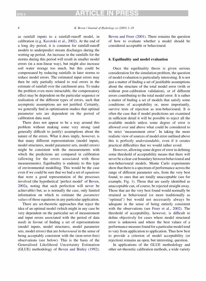
Fig. 1. Dotty plots (projections of points on a likelihood surface onto a single parameter axis) resulting from Monte Carlo realisations of

parameter sets for the MAGIC Long Term Soil Acidification and Water Quality Model (after Page et al., 2003). Only six out of 12 parameters

varied shown. Model evaluation based on joint fuzzy membership function as to whether modelled concentrations fall within acceptable limits

for several specific points in time.

K. Beven / Journal of Hydrology xx (2005) 1–192


the search for an ‘optimum’ but at the risk of avoiding

important issues of model acceptability and uncer-

tainty). This manifesto is an attempt to provide a

convincing case as to why it should be embraced in

future.

There is a very important issue of modelling

philosophy involved that might explain some of the

reluctance to accept the thesis. Science, including

hydrological science, is supposed to be an attempt to

work towards a single correct description of reality. It

is not supposed to conclude that there must be

multiple feasible descriptions of reality. The users of

research also do not (yet) expect such a conclusion

and might then interpret the resulting ambiguity of

predictions as a failure (or at least an undermining) of

the science. This issue has been addressed directly by

Beven (2002a) who shows that equifinality of

representations is not incompatible with a scientific

K. Beven / Journal of Hydrology xx (2005) 1–19 3


research program, including formal hypothesis test-

ing. In that paper, the modelling problem is presented

as a mapping of the landscape into a space of feasible

models (structures as well as parameter sets). The

uncertainty does not lie in the predictions within this

model space since the parameters in that space are

known (even for a space of stochastic model

structures). The dominant uncertainty lies in how to

map the real system into that space of feasible models

(Beven, 2000, 2001a). Mapping to an ‘optimal’ model

is equivalent to mapping to a single point in the model

space. Statistical evaluation of the covariance struc-

ture of parameters around that optimal model is

equivalent to mapping to a small contiguous region of

the model space. Mapping of Pareto optimal models is

equivalent to mapping to a front or surface in the

space of performance measures but which might be a

complex manifold with breaks and discontinuities

when mapped into in the model space. But, computer

intensive studies of responses across the model space

have shown that these mappings are too simplistic,

since they arbitrarily exclude many models that are

very nearly as good as the ‘optima’. For any

reasonably complex model, acceptably good fits are

commonly found much more widely than just in the

region of the ‘optimum’ or Pareto ‘optima’ (quotation

marks are used here because the apparent global

optimum may change significantly with changes in

calibration data, errors in input data or performance

measure).

This also brings attention to the problem of model

evaluation and the representation of model error. The

GLUE methodology has been commonly criticised

from a statistical inference viewpoint for using

subjective likelihood measures and not using a formal

representation of model error (e.g. Clarke, 1994;

Thiemann et al., 2001; and many different referees).

For ideal cases, this can mean that non-minimum error

variance (or non-maximum likelihood) solutions

might be accepted as good models, that the resulting

likelihoods do not provide the true probabilities of

predicting an output given the model, while the

parameter estimates might be biased by not taking the

correct structural model of the errors into account in

the likelihood measure. In fact, the GLUE method-

ology is general in that it can use ‘formally correct’

likelihood measures if this seems appropriate (see

Romanowicz et al., 1994; Romanowicz and Beven,

1996; and comments by Beven and Young, 2003), but

need not require that any single model is correct (and

correct here normally means not looking too closely at

some of the assumptions made about the real errors in

formulating the likelihood function, even if, in

principle, those assumptions can be validated).

The difference is again one of philosophy. It is

commonly forgotten that statistical inference methods

were originally developed for fitting distributions to

data in which the modelling errors can be treated as

measurement errors, assuming that the chosen

distributional form is correct. The approach is easily

extended to regression and other more complex

inference problems, but in each case, it is assumed

that the model structure is correct and that the model

errors can be treated as simple additive (or multi-

plicative if treated in log transform) measurement

errors (see the difficulties that this can lead to in the

discussion, for example, by Draper, 1995). Tech-

niques such as reversible jump Monte Carlo Markov

Chain methods have been developed to try to evaluate

and combine the predictions of many potential model

structures but in each case each individual model is

treated as if it were correct. The ‘measurement error’

terminology is still in use today in the calibration of

complex simulation models (e.g. Thiemann et al.,

2001 slip into this usage (p. 2525) even though

elsewhere they make clear the multiple sources of

error), despite the fact that input data errors, model

structural errors and other sources of error mean that

the model errors are often much larger than sensible

assumptions about measurement errors and despite

the evidence that there may not be a clear optimum in

the model space.

So what are the implications of taking an

alternative view, one in which it is accepted that the

hydrological model (and the error model) may not be

structurally correct and that there may not be a clear

optimal model, even when multiple performance

measures are considered? This situation is not rare

in hydrological modelling. It is commonplace. It

should, indeed, be expected because of the over-

parameterisation of hydrological models, particularly

distributed models, relative to the information content

of observational data available for calibration of

parameter values (even in research catchments). But

modellers rarely search for good models that are not

‘optimal’. Nor do they often search for reduced



dimensionality models that would provide equally

good predictions but which might be more robustly

estimated (e.g. Young, 2002). Nor do they often

consider the case where the ‘optimal’ model is not

really acceptable (see, for example, Freer and K,

2002); it is, after all, the best available.

This paper tries to address some of these problems

in the form of a manifesto for a future research

programme. It starts with a brief summary of the

causes of equifinality. It then considers the problem of

parameter and uncertainty estimation in the ideal case

of the perfect model. More realistic non-ideal cases

are then discussed, together with techniques for model

evaluation. The important issues of separation of

uncertainties and model order reduction are identified

as important for future research.

2. Equifinality, ambiguity, non-uniqueness,

ill-posedness and identifiability

The equifinality thesis is intended to focus

attention on the fact that there are many acceptable

representations that cannot be easily rejected and that

should be considered in assessing the uncertainty

associated with predictions. The concept owes a lot to

the HSY analysis of multiple behavioural models in

sensitivity analysis. The term equifinality has a long

history in geomorphology, indicating that similar

landforms might arise as a result of quite different sets

of processes and histories. Thus from the landform

alone, without additional evidence, it might be

difficult to identify the particular set of causes or to

differentiate different feasible causes (see discussion

in Beven, 1996). The term was also used in the text of

General Systems Theory of von Bertalanffy (1968)

and was adopted for the environmental modelling

context by Beven (1993). Implicit in this usage, is the

rejection of the assumption that a single correct

representation of the system can be found given the

normal limitations of characterisation data.

For any particular set of observations, of course,

some of those acceptable or behavioural models will

be better in terms of one or more performance

measures. The important point, however, is that

given the sources of error in the modelling process,

the behavioural models cannot easily be rejected as

feasible representations of the system given the level

of error in representing the system. In one sense, this

can be viewed as a problem of decidability between

feasible descriptions (hypotheses) of how the hydro-

logical system is working (Beven, 2002a).

Decidability between models in hypothesis testing

raises an interesting issue, however, linked to the

information content of calibration data. To be able to

represent different hypotheses about the processes of a

hydrological system, it is necessary to have represen-

tations or parameterisations of those processes. This is

why there has been a natural tendency for models to

grow in complexity. Additional complexity will

generally require additional numbers of parameters

to be defined, the values of which will require

calibration—but often without additional data being

collected with the aim of determining those values.

Thus, testing different hypotheses will tend to lead to

more overparameterisation and equifinality and it

should be expected that even if we could define the

mathematically ‘perfect’ model, it will still be subject

to equifinality if driven with non-error-free initial and

boundary conditions and compared with non-error-

free output measurements.

Environmental models are therefore mathemat-

ically ill-posed or ill-conditioned (Beck, 1987). The

information content available to define a modelling

problem does not allow a single or unambiguous

mathematical solution to the identification problem.

Non-uniqueness in model identification, particular for

models that are complex relative to the quantity and

quality of data available for model calibration, has

also been used widely to indicate that multiple models

might give equally acceptable fits to observational

data. It has been primarily used in the discussion of

the difficulties posed in parameter calibration for

response surfaces that show many local mimima, one

of which may be (marginally) the global optimum, at

least for that set of observations. Non-uniqueness

(also non-identifiability) has usually been seen as a

difficulty in finding the global optimal model and, by

implication, the true representation of the system. It

has not been viewed as an intrinsic characteristic of

the modelling process.

Ambiguity has also been used to reflect model

identification problems in a variety of ways. Beck and

Halfon (1991) refer to ambiguity in distinguishing

models identified on the same data set that have

overlapping prediction limits. It is used somewhat



differently by Zin (2002) to denote models for which

predictions made with different stochastic realisations

of the input data that cannot be distinguished

statistically. Ambiguity is perhaps a less contentious

word than equifinality but here the use of the latter is

intended to emphasise that, given the normal

limitations on the data for model evaluation, the

decidability problem may be greater than statistical

ambiguity between parameter sets but may also

extend to real differences in process explanation

when multiple model structures (or multiple function-

ality within a model structure) are considered.

Equifinality, ambiguity and non-uniqueness have

been discussed in this section with respect to the

identifiability of models, parameter values and sets of

parameter values. These terms are very often used in

this way by modellers. It is, however, worth noting

that there is another sense in which identifiability can

be used in respect of environmental systems, i.e.

whether the dominant modes of response of the

system are identifiable. Hydrological systems, for

example, often show relatively simple impulse

response characteristics that can often be surprisingly

well approximated by a linear transfer function (or

unit hydrograph), even if the system gain may be non-

stationary or non-linear and difficult to predict (but see

Young, 1998, 2001, 2003; Young et al., 2004;

Bashford et al., 2002; Young and Parkinson, 2002).

Where there is a dominant mode of response, it may

well be possible to identify it relatively unambigu-

ously. In one sense, the various parametric models

that can be used to represent that response, with all

their potential for equifinality and different process

interpretations, are just different attempts to simulate

the same response characteristics of the system. The

ambiguity lies not in the system itself, but only in

deciding about different representations of it (see for

example, the different explanations of ‘fractal’

residence time distributions in Kirchner et al., 2001).

3. Equifinality and the deconstruction of model

error

That is not to say that any model error is arising

totally from the different model representations of the

system (model structures and parameter sets). There is

a problem, in any modelling application, of trying to

understand the origins of the error between model

predictions of a variable and any observational data of

the same variable. The difficulty comes because there

are a variety of sources for the error but, at any given

time, only one measure of the deviation or residual

between prediction and observation at a site (i.e. the

‘model error’). Multiple observation sites or perform-

ance measures can, of course, produce conflicting

prediction errors (an improvement in one prediction

results in a deterioration in another). Thus, decon-

struction of the error into its source components is

difficult, particularly in cases common in hydrology

where the model is non-linear and different sources of

error may interact in a non-linear way to produce the

measured deviation Beven, 2004b,c). There are

obvious sources of error in the modelling process,

for example, the error associated with the model

inputs and boundary conditions, the error associated

with using an approximate model of the real

processes, and the error associated with the observed

variable itself.

There are also some less obvious sources of error,

such as the variable predicted by a model not being

the same quantity as that measured, even though they

might be referred to by the same name, because of

heterogeneity and scale effects, non-linearities or

measurement technique problems (the incommensur-

ability problem of Beven, 1989). A soil moisture

variable, for example, might be predicted as an

average over a model grid element several metres in

spatial extent and over a certain time step; the same

variable might be measured at a point in space and

time by a small gravimetric sample, or by time

domain reflectrometry integrating over a few tens of

cm, or by a cross-borehole radar or resistivity

technique, integrating over several metres. Only the

latter might be considered to approach the same

variable as predicted by the model, but may itself be

subject to a model inversion that involves additional

parameters in deriving an estimate of soil moisture

(see, for example, the discussion of instrument filters

by Cushman, 1986, though this is not easily applied in

non-linear cases).

In rainfall-runoff modelling, the predictions are

most usually compared with the measured discharges

at the outlet from a catchment area. This may be

considered to be the same variable as that predicted by

the model, although it may be subject to measurement



errors due to underflow or bypassing and rating curve

inaccuracies, especially at very high and very low

flows.

Since it is difficult to separate the sources of error

that contribute to model error, as noted above it is

often assumed to be adequately treated as a single

lumped additive variable in the form:

QðX; tÞZMðQ;X; tÞC3ðX; tÞ (1)

where Q(X, t) is a measured variable, such as

discharge, at point X and time t; M(Q, X, t) is the

prediction of that variable from the model with

parameter set Q; and 3(X, t) is the model error at

that point in space and time. Transformations of the

variables of Eq. (1) can also be used where this seems

more appropriate to constrain the modelling problem

to this form. Normal statistical inference then aims to

identify the parameter set Q that will be in some sense

optimal, normally by minimising the residual error

variance of a model of the model error, that might

include its own parameters for bias and autocorrela-

tion terms with the aim of making the residual error

iid. This additive form allows the full range of

statistical estimation techniques, including Bayesian

updating, to be used in model calibration. The

approach has been widely used in hydrological and

water resources applications, including flood fore-

casting involving data assimilation (e.g. Krzysztofo-

wicz, 2002; Young, 2002 and references therein);

groundwater modelling, including Bayesian aver-

aging of model structures (e.g. Neuman, 2003; Ye

et al., 2004); and rainfall-runoff modelling (e.g.

Kavetski et al., 2002; Vrugt et al., 2003).

In principle, the additive error assumptions that

underlies this form of uncertainty is particularly

valuable for two reasons: that it allows checking of

whether the actual errors conform to the assumptions

made about the structural model of the errors and that,

if this is so, then a true probability of predicting an

observation, conditional on the model can be

predicted. These advantages, however, may be

difficult to justify in many real applications where

poorly known input errors are processed through a

non-linear model subject to structural error and

equifinality (see Hall, 2003, for a brief review of a

more generalised mathematisation of uncertainty,

including discussion of fuzzy set methods and the

Dempster–Shafer theory of evidence). One impli-

cation of the limitations of the additive error model is

that it may actually be quite difficult to estimate the

true probability of predicting an observation, given

one or more models, except in ideal cases.

4. Ideal cases: theoretical estimation of uncertainty

There are many studies in the hydrological

literature, dating back to at least Ibbitt and O’Donnell

(1971) and continuing to at least Thiemann et al.

(2001), where the effects of errors of different types on

the identification of model parameters have been

studied based on hypothetical simulation where it is

known that the model is correct. This is the ideal case.

A model run is made, given a known input series and

known parameters, to produce a noise free set of

‘observations’. The input data and observations are

then corrupted by different assumed error models,

generally with simple Gaussian structure, and a

parameter identification technique is used to calibrate

themodel to seewhether the original parameters can be

recovered in the face of different types and levels of

corruption. Any concerns about the level of model

structural error can be neglected in such cases. The

argument is that any model identification procedure

should be shown towork for error corrupted ideal cases

so that the user can havemore faith in such a procedure

in actual applications. This argument depends, how-

ever, on the application in practice not being distorted

by model structural error (see Section 5).

If the errors are indeed Gaussian in nature, or can

be transformed to be, then the full power of statistical

likelihood theory can be used. The simplest assump-

tion, for the simulation of a single variable over a

number of time steps (T) is that the errors 3(t) are an

independent and identically distributed Gaussian

variable with zero mean and constant variance.

Then, the probability of predicting a value of Q(t)

given the model M(Q) based on the additive model of

Eq. (1) is given by:

LðQjMðQÞÞf ðs2eÞKT=2expðs2e =s

2oÞ (2)

where s2e is the variance of the error series, s2o is the

variance of the observations, and T is the number of

time steps.



The variance of the parameter estimates based on

this likelihood function can be obtained from

evaluating the Hessian of the log likelihood function

at the point where the variance of the error series is

minimised (or more generally where the log

likelihood is maximised). Note, however, that for

non-linear models this will not produce the same

result as evaluating (2) for every combination of

parameters and using the estimate of the local error

variance, even in the immediate region of the

optimum. In this case, a more direct evaluation of

the nature of the likelihood surface using Monte

Carlo, or Monte Carlo Markov Chain (MC2) sampling

techniques would be advantageous (e.g. Kuczera and

Parent, 1998; Vrugt et al., 2002).

For this ideal case, if the model fits the data very

well and the error variance is very small, the

likelihood function will be very peaked. This will be

especially so if the model fits well over a large number

of time steps (note the power of T/2 in Eq. (2)). The

resulting variance of the parameter estimates will be

very small. This arises out of the theory, regardless of

whether there are other model parameter sets that

produce error variances that are very nearly as small

elsewhere in the model space.

This is a consequence of the implicit assumption

that the optimal model is correct. In hypothetical ideal

cases this is clearly so; but it is not such a good

assumption in hydrological modelling of real catch-

ment, groundwater or water quality systems. Simple

assumptions about the error structures are convenient

in applying statistical theory but are not often borne

out by actual series of model errors which may show

changing bias, changing variance (heteroscedasticity),

changing skew, and changing correlation structures

under different hydrological conditions (and for

different parameter sets). It is known for linear

systems that ignoring such characteristics, or wrongly

specifying the structure of the error model, will lead to

bias in the estimates of parameter values. The same

will be the case for non-linear systems, but there is

then no guarantee that, for example, Gaussian errors

in model inputs will lead to an additive Gaussian error

model of the form of Eq. (1).

There are ways of dealing with complex error

structures within statistical likelihood theory; one is to

try and account for the nature of the structure by

making the model of the errors more complex.

For example, methods to estimate a model inadequacy

function have been proposed by Kennedy and

O’Hagen (2001) and to deal with heteroscedasticity

by transformation (e.g. Box and Cox, 1964). The aim

is to produce an error series that has a constant

variance and (relative) independence in time and

space to allow the various parameters and correction

terms to be more easily estimated.

In all these approaches, the implicit assumption

that the model is correct remains and leaves open the

possibility for the (non-physical) structural model of

the errors compensating for errors in the model

structure and from other sources (Beven, 2004c).

Other feasible models that provide acceptable

simulations are then commonly neglected. The

interest is only in efficiently identifying that true

model as some optimum in the space of feasible

models. This is understandable in the ideal case

because it is known that a ‘true’ model exists. It does

not necessarily follow that those other acceptable

models are not of interest in more realistic cases

where the possibility of model structural error may

undermine the assumption that the model is correct (or

more generally that the effects of model structural

error can be treated simply as a linear contribution to

the total model error of Eq. (1)).

5. Realistic cases: compensation of uncertainty

In more realistic cases, it is not possible to assume

that the model structure is correct nor is it possible to

separate the different sources of model uncertainty.

We can assess the series of total model errors in space

and time that results from the individual sources of

errors in conjunction with the effects of model

structural error. In fact, even the true measurement

error is independent of model structural error only for

the case where predicted variables and observed

variables are truly commensurate. If scale, non-

linearity and heterogeneity issues arise in comparing

predictions with measurements then the effective

measurement error may also interact with model

structural error.

There is then significant possibility for calibrated

parameter values to compensate for different types of

error, perhaps in complex ways. An obvious example

is where it is attempted to adjust an input series, such



as rainfall inputs to a rainfall-runoff model, in

calibration (e.g. Kavetski et al., 2002). At the end of

a long dry period, it is common for rainfall-runoff

models to underpredict stream discharges during the

wetting up period. An increase in the rainfalls for the

storms during this period will result in smaller model

errors (in a non-linear way), but might also increase

soil water storage too much, but this could be

compensated by reducing rainfalls in later storms to

reduce model errors. The estimated input errors may

then be only partially related to real errors in the

estimate of rainfall over the catchment area. To make

the problem even more intractable, the compensatory

effect may be dependent on the particular sequence or

realisation of the different types of errors, such that

asymptotic assumptions are not justified. Certainly,

we generally find in optimisation studies that optimal

parameter sets are dependent on the period of

calibration data used.

There does not appear to be a way around this

problem without making some very strong (and

generally difficult to justify) assumptions about the

nature of the errors. What it does imply, however, is

that many different representations (model inputs,

model structures, model parameter sets, model errors)

might be consistent with the measurements with

which the predictions are compared in calibration

(allowing for the errors associated with those

measurements). Equifinality is endemic to this type

of environmental modelling. This would be the case

even if we could be sure that we had a set of equations

that were a good representation of the processes

involved (the hypothetical ‘perfect model’ of Beven,

2002a, noting that such perfection will never be

achievable) but, as is normally the case, only limited

information on which to estimate the parameter

values of those equations in any particular application.

There are set-theoretic approaches that reject the

idea of an optimal model (which might in any case be

very dependent on the particular set of measurement

and input errors associated with the period of data

used) in favour of finding a set of representations

(model inputs, model structures, model parameter

sets, model errors) that are behavioural in the sense of

being acceptably consistent with the (non-error-free)

observations (see below). This is the basis of the

Generalised Likelihood Uncertainty Estimation

(GLUE) methodology of Beven and Binley (1992);

Beven and Freer (2001). There remains the question

of how to evaluate whether a model should be

considered acceptable or behavioural.

6. Equifinality and model evaluation

Once the equifinality thesis is given serious

consideration for the simulation problem, the question

of model evaluation is particularly interesting. It is not

just a matter of finding a set of justifiable assumptions

about the structure of the total model error (with or

without post-calibration validation), or of different

errors contributing to the total model error. It is rather

a matter of finding a set of models that satisfy some

conditions of acceptability or, more importantly,

survive tests of rejection as non-behavioural. It is

often the case that if model predictions are examined

in sufficient detail it will be possible to reject all the

available models unless some degree of error is

allowed over and above what could be considered to

be strict ‘measurement error’. In taking the more

realistic view of sources of model error outlined above

this is perfectly understandable, even if it creates

practical difficulties that we would rather avoid.

However, allowing some degree of error in defining

some threshold of acceptability means that there will

never be a clear-cut boundary between behavioural and

non-behavioural models. Monte Carlo experiments

show that there is a spectrum of performance across the

range of different parameter sets, from the very best

found, to ones that are totally unacceptable (see for

example, Fig. 1). Those that are easily identified as

unacceptable can, of course, be rejected straight away.

Those that are the very best found would normally be

retained as behavioural (or more traditionally as

‘optimal’) but would not necessarily always be

adequate in the sense of being entirely consistent

with the observations (see Freer et al., 2002). The

threshold of acceptability, however, is difficult to

define objectively for cases where model structural

error is unknown and where the best values of a

performancemeasure found for a particularmodel tend

to vary from application to application. Thus how best

to provide a criterion of model acceptability (or

rejection) remains an open, but interesting, question.

In applications of the GLUE methodology and

other set-theoretic calibration methods, a wide variety



of performance measures and rejection criteria have

been used in the past. All can be considered as a way

of mapping of the hydrological system of interest into

a model space (Beven, 2002a,b). Initially, the

mapping will be highly uncertain but as more

information about the system becomes available,

then it should be easier to identify those parts of the

model space that give behavioural simulations. The

approach is sufficiently general to subsume both

traditional optimisation (mapping to a single point in

the model space); stochastic identification (mapping

to a small region controlled by the identified

covariance structure); the equifinality thesis if all

behavioural model structures and parameter sets are

considered; and hypothesis testing or Bayesian

updating in refining the mapping (Beven, 2002a,b;

Beven and Young, 2003).

7. Set theoretic methods for model evaluation

Monte Carlo based set-theoretic methods for

model calibration and sensitivity analysis have been

used in a variety of disciplines for some 50 years. The

first use in geophysics was perhaps that of Press

(1968) where a model of the structure of the earth was

evaluated in the light of knowledge about 97

eigenperiods, travel times of compressional and

shear waves, and the mass and moment of inertia of

the earth. Parameters were selected randomly from

within specified ranges for 23 different depths, which

were then interpolated to 88 layers within a spherical

earth. Ranges of acceptability were set for the

predictions to match these observational data. These

were applied successively within a hierarchical

sampling scheme for the compressional, stress and

density parameters. Five million models were eval-

uated of which six passed all the tests (although of

those three were then eliminated as implausible

because of having a negligible density gradient in

the deep mantle). The ‘standard model’ of the time

was also rejected on these tests. Subjective choices

were made both of the sampling ranges for the

parameters and for the multiple limits of acceptability.

Those choices are made explicit, and are therefore

open to discussion (indeed, Press discusses an

additional constraint that might be evoked to refine

the results to a single model but notes that ‘while

reasonable, it is not founded in either theory or

experiment’, p. 5233).

Use of this type of Monte Carlo method in

hydrology and water quality modelling dates back

(at least) to the 1970s (Whitehead and Young, 1979;

Hornberger and Spear, 1981; Gardner and O’Neill,

1983; Young, 1983). In many studies, the set of

feasible models has been defined a priori and the

Monte Carlo realisations are then used as a means of

propagating prediction uncertainties in a non-linear

modelling context. The more interesting question,

however, is to let the available observations condition

the behavioural models, without making strong prior

assumptions about the parameter distributions or

feasible models. This was the essence of the

Generalised Sensitivity Analysis of Hornberger and

Spear (1981) which was based on assessing all the

model realisations into the set of behavioural models

and the set of non-behavioural models according to

some ranking of model performance. Such studies

rapidly found, however, that in many cases there will

be no clear demarcation between behavioural and

non-behavioural models and, in the case of Hornber-

ger et al. (1985), resort was made to declaring the top

30% as behavioural in a preliminary sensitivity

analysis.

Multiple measures, as in the Press (1968) study,

should help in this respect, if a behavioural model is

required to satisfy some prior limits of acceptability

(see also Hornberger and Spear, 1981). It is possible to

define multiple performance measures for a single

predicted variable such as discharge (sum of squared

errors, sum of absolute errors in peak discharge, sum

of squared log errors etc. see for example Parkin et al.,

1996) but more information will be added to the

conditioning process if a model can be evaluated with

respect to distributed observations or multiple

chemistry characteristics in water quality.

This does, however, also introduce additional

difficulties as soon as it is realised that local

observations might require local parameter values to

represent adequately the local responses unless

generous limits of acceptability are used to allow for

the difference in meaning between the prediction at a

point by a model using global parameter values (and

non-error free input data and model structures) and a

local observation. In distributed groundwater model-

ling, this type of model evaluation suggests that



equifinality is endemic to the problem (see Feyen et

al., 2001; Binley and Beven, 2003). Similarly, in

rainfall-runoff modelling, the use of distributed

observational information (disappointingly) does not

appear to help much in eliminating the equifinality

problem (see Lamb et al., 1998; Blazkova et al., 2002;

Blazkova and Beven, 2003; Christiaens and Feyen,

2002).

8. Extending the concept of the behavioural model

The concept of such set-theoretic model evaluation

is simple. Models that do not fall within the multiple

prior limits of acceptability should be rejected. This

allows the possibility of many feasible models

satisfying the limits of acceptability and being

accepted as behavioural. It also, however, allows the

possibility that none of the models tried will satisfy

the limits of acceptability. This was the case for the

distributed hydrological model in Parkin et al. (1996),

where all parameter sets failed 10 out of 13 limits of

acceptability, and for the application of TOPMODEL

reported in Freer et al., 2002. It was also the case for a

model of the algal dynamics in Lake Veluwe reported

in Van Straten and Keesman (1991). They had to

increase their limits of acceptability by 50% to obtain

any behavioural realisations of the simplest model

tried, ‘to accommodate the apparent structural error’

(p. 175) (their application may also have suffered

from incommensurability and input realisation

errors).

Thus, any model evaluation of this type needs to

take account of the multiple sources of model error

more explicitly. As noted above, this is difficult for

realistic cases. Simplifying the sources of error to

input errors, model structural errors and true

measurement errors is not sufficient because of the

potential for incommensurability between observed

and predicted variables. There is no general theory

available for doing this in non-linear dynamic cases.

Most modellers simply assume that they are the same

quantity, even where this is clearly not the case. Thus,

in assessing model acceptability it is really necessary

to decide on an appropriate level of ‘effective

observation error’ that takes account of such

differences. When defined in this way, the effective

observation error need not have zero mean or constant

variance, nor need it be Gaussian in nature,

particularly where there may be physical constraints

on the nature of that error. Once this as been done,

then it should be required that any behavioural model

should provide all its predictions within the range of

this effective observational error. Thus a model will

be classified as acceptable if:

QminðX; tÞ!MðQ;X; tÞ!QmaxðX; tÞ

for all QðX; tÞ(3)

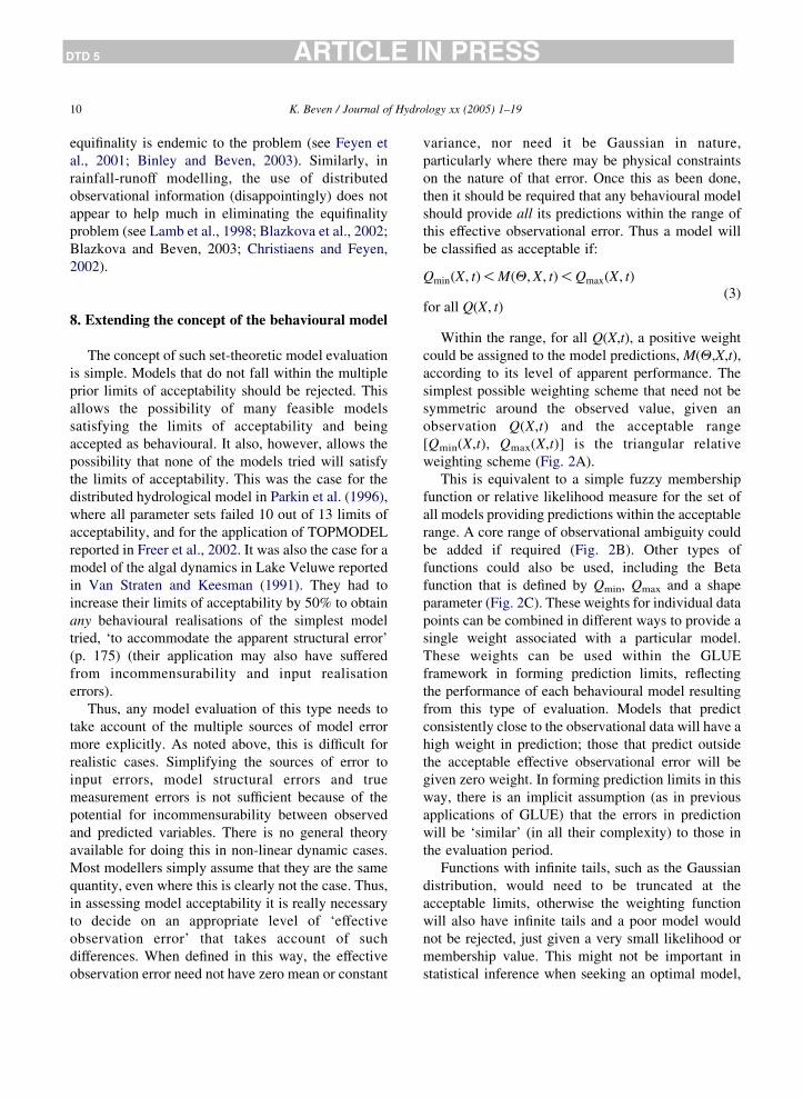
Within the range, for all Q(X,t), a positive weight

could be assigned to the model predictions, M(Q,X,t),

according to its level of apparent performance. The

simplest possible weighting scheme that need not be

symmetric around the observed value, given an

observation Q(X,t) and the acceptable range

[Qmin(X,t), Qmax(X,t)] is the triangular relative

weighting scheme (Fig. 2A).

This is equivalent to a simple fuzzy membership

function or relative likelihood measure for the set of

all models providing predictions within the acceptable

range. A core range of observational ambiguity could

be added if required (Fig. 2B). Other types of

functions could also be used, including the Beta

function that is defined by Qmin, Qmax and a shape

parameter (Fig. 2C). These weights for individual data

points can be combined in different ways to provide a

single weight associated with a particular model.

These weights can be used within the GLUE

framework in forming prediction limits, reflecting

the performance of each behavioural model resulting

from this type of evaluation. Models that predict

consistently close to the observational data will have a

high weight in prediction; those that predict outside

the acceptable effective observational error will be

given zero weight. In forming prediction limits in this

way, there is an implicit assumption (as in previous

applications of GLUE) that the errors in prediction

will be ‘similar’ (in all their complexity) to those in

the evaluation period.

Functions with infinite tails, such as the Gaussian

distribution, would need to be truncated at the

acceptable limits, otherwise the weighting function

will also have infinite tails and a poor model would

not be rejected, just given a very small likelihood or

membership value. This might not be important in

statistical inference when seeking an optimal model,

0

0.2

0.4

0.6

0.8

1

0

0.2

0.4

0.6

0.8

1

0

0.2

0.4

0.6

0.8

1

1.2 1.4 1.6 1.8 2 2.2

1.2 1.4 1.6 1.8 2 2.2

1.2 1.4 1.6 1.8 2 2.2

A

B

C

Fig. 2. Defining acceptable error around an observed value (vertical

line), with the observed value, Q, not central to the acceptable

range, Qmin to Qmax. (A) Triangular, with peak at observation. (B)

Trapezoidal, with inner core range of observational ambiguity. (C).

Beta distribution with defined range limits.



but it is important in this context when trying to set

limits for acceptable models. For those models that

meet the criteria of (3) and are then retained as

behavioural, all the methods for combining such

measures available from Fuzzy Set Theory are

available (e.g. Klir and Folger, 1988; Ross, 1995).

Other possibilities of taking account of the local

deviations between observed and predicted quantities

for the behavioural models, might also be used.

This methodology gives rise to some interesting

possibilities. If a model does not provide predictions

within the specified range, for any Q(X,t), then it

should be rejected as non-behavioural. Within this

framework there is no possibility of a representation

of model error being allowed to compensate for poor

model performance, even for the ‘optimal’ model. If

there is no model that proves to be behavioural then it

is an indication that there are conceptual, structural or

data errors (though it may still be difficult to decide

which is the most important). There is, perhaps, more

possibility of learning from the modelling process on

occasions when it proves necessary to reject all the

models tried.

This implies that consideration also has to be given

to input and boundary condition errors, since, as noted

before, even the ‘perfect’ model might not provide

behavioural predictions if it is driven with poor input

data error. Thus, it should be the combination of

input/boundary data realisation (within reasonable

bounds) and model parameter set that should be

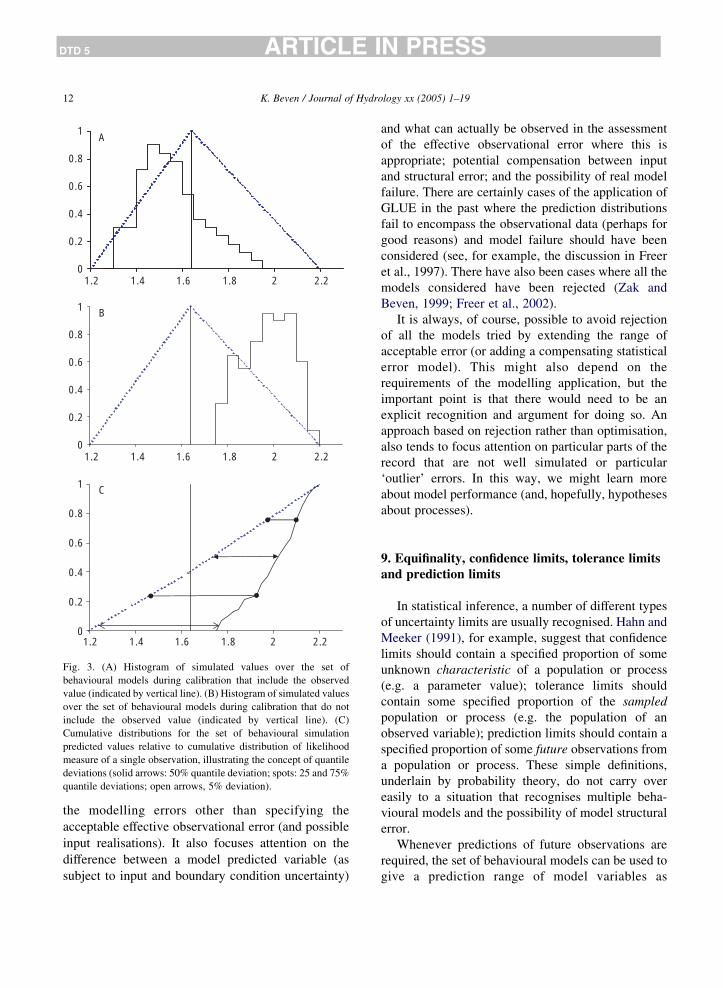
evaluated against the observational error. The result

will (hopefully) still be a set of behavioural models,

each associated with some likelihood weight

(Fig. 3A). Any compensation effect between an

input realisation (and initial and boundary conditions)

and model parameter set in achieving success in the

calibration period will then be implicitly included in

the set of behavioural models.

There is also the possibility that the behavioural

models defined in this way do not provide predictions

that span the range of the acceptable error around an

observation (Fig. 3B). The behavioural models might,

for example, provide simulations of an observed

variable Q(X,t) that all lie in the range Q(X,t) to

Qmax(X,t), or even just a small part of it. They are all

still acceptable, but are apparently biased. This

provides real information about the performance of

the model (and/or other sources of error) that can be

investigated and allowed for specifically at that site in

prediction (the information on the quantile deviations

of the behavioural models, as shown in Fig. 3C, can be

preserved, for example). Time series of these quantile

deviations might provide useful information on how

the model is performing across a range of predictions.

This seems to provide a very natural approach to

model calibration and evaluation, that avoids

making difficult assumptions about the nature of

A

B

C

0

0.2

0.4

0.6

0.8

1

1.2 1.4 1.6 1.8 2 2.2

0

0.2

0.4

0.6

0.8

1

1.2 1.4 1.6 1.8 2 2.2

0

0.2

0.4

0.6

0.8

1

1.2 1.4 1.6 1.8 2 2.2

Fig. 3. (A) Histogram of simulated values over the set of

behavioural models during calibration that include the observed

value (indicated by vertical line). (B) Histogram of simulated values

over the set of behavioural models during calibration that do not

include the observed value (indicated by vertical line). (C)

Cumulative distributions for the set of behavioural simulation

predicted values relative to cumulative distribution of likelihood

measure of a single observation, illustrating the concept of quantile

deviations (solid arrows: 50% quantile deviation; spots: 25 and 75%

quantile deviations; open arrows, 5% deviation).



the modelling errors other than specifying the

acceptable effective observational error (and possible

input realisations). It also focuses attention on the

difference between a model predicted variable (as

subject to input and boundary condition uncertainty)

and what can actually be observed in the assessment

of the effective observational error where this is

appropriate; potential compensation between input

and structural error; and the possibility of real model

failure. There are certainly cases of the application of

GLUE in the past where the prediction distributions

fail to encompass the observational data (perhaps for

good reasons) and model failure should have been

considered (see, for example, the discussion in Freer

et al., 1997). There have also been cases where all the

models considered have been rejected (Zak and

Beven, 1999; Freer et al., 2002).

It is always, of course, possible to avoid rejection

of all the models tried by extending the range of

acceptable error (or adding a compensating statistical

error model). This might also depend on the

requirements of the modelling application, but the

important point is that there would need to be an

explicit recognition and argument for doing so. An

approach based on rejection rather than optimisation,

also tends to focus attention on particular parts of the

record that are not well simulated or particular

‘outlier’ errors. In this way, we might learn more

about model performance (and, hopefully, hypotheses

about processes).

9. Equifinality, confidence limits, tolerance limitsand prediction limits

In statistical inference, a number of different types

of uncertainty limits are usually recognised. Hahn and

Meeker (1991), for example, suggest that confidence

limits should contain a specified proportion of some

unknown characteristic of a population or process

(e.g. a parameter value); tolerance limits should

contain some specified proportion of the sampled

population or process (e.g. the population of an

observed variable); prediction limits should contain a

specified proportion of some future observations from

a population or process. These simple definitions,

underlain by probability theory, do not carry over

easily to a situation that recognises multiple beha-

vioural models and the possibility of model structural

error.

Whenever predictions of future observations are

required, the set of behavioural models can be used to

give a prediction range of model variables as



conditioned on the process of model evaluation. The

fuzzy (possibilistic) or probabilistic weights associ-

ated with each model can be used to weight the

predictions to reflect how well that particular model

has performed in the past. The weights then control

the form of a cumulative density (possibility) function

for any predicted variable over the complete set of

behavioural models, from which any desired predic-

tion limits can be obtained. The weights can be

updated as new observations are used to refine the

model evaluation. This is the essence of the GLUE

methodology and of other set theoretic approaches to

model prediction (e.g. Beven and Freer, 2001).

Note, however, that while it is necessary to assume

that the behavioural models in calibration will also be

behavioural in prediction, this procedure only (at best)

gives the tolerance limits (in the calibration period) or

the prediction limits of the weighted simulations of

any variable. These prediction limits will be con-

ditional on the choice of limits of acceptability; the

choice of weighting function; the range of models

considered; any prior weights used in sampling

parameter sets; the treatment of input data error, etc.

All these components of estimating the uncertainty in

the predictions must, at least, be made explicit.

However, given the potential for input and model

structural errors, they will not guarantee that a

specified proportion of observations, either in cali-

bration or future predictions, will lie within the

tolerance or prediction limits (the aim, at least, of a

statistical approach to uncertainty). Nor is this

necessarily an aim in the proposed framework. In

fact, it would be quite possible for the tolerance limits

over all the behavioural models to contain not a single

observed value in the calibration period (as in

Fig. 3B), and yet for all of those models to still

remain behavioural in the sense of being within some

specified acceptable error limits for all observed

quantities. The same could clearly be true in

prediction of future observations, even if the

assumption that the models remain behavioural in

prediction is valid.

Similar considerations apply in respect of the

confidence limits for a parameter of the model. Again,

it is simple to calculate likelihood weighted marginal

distributions of any parameter over all the behavioural

models. The marginal distributions can have a useful

role in assessing the sensitivity of model outputs to

individual parameters (e.g. Hornberger and Spear,

1981; Young, 1983; Beven and Binley, 1992; Beven

and Freer, 2001). For each of those models, however,

it is the parameter set that results in acceptable

behaviour. It is quite possible to envisage a situation

in which a parameter set based on the modal value of

each of the parameter marginal distributions is not

itself behavioural (even if this might be an unlikely

scenario). Any confidence limits for individual

parameters derived from these marginal distributions

therefore cannot have the same meaning as in

traditional inference (in the same way that the use of

likelihood has been generalised within this frame-

work). Marginal parameter quantiles can, however, be

specified explicitly.

This account of the different uncertainty limits

raises a further issue in prediction as to how best to

take account of any information on deviations

between the behavioural model predictions and

observed quantities (as demonstrated in Fig. 3C).

One approach is the use of probabilistic weights

based on a formal likelihood function is then a

special case of this procedure for cases where

strong (normally Gaussian, with or without bias,

heteroscedasticity and autocorrelation) assumptions

about the error structure can be justified (see

Romanowicz et al., 1996, who used classical

likelihood measures within the GLUE framework).

The advantage of doing so is that a formal

likelihood function takes account of the residual

error in predicting an observed value given the

model. The difficulties in doing so are that it adds

error model parameters to be identified and that

there is no reason to expect that the structural

model of the errors should be Gaussian or the same

across all the behavioural models (albeit that these

are often used as convenient assumptions).

As noted above, an alternative approach based on

preserving calibration information on quantile devi-

ations of the behavioural models might be possible.

This can be done in a consistent way for any particular

observation by transforming the prediction quantiles

of the behavioural models to the fuzzy membership

function that defines model acceptability (Fig. 3C). In

prediction, it would then still be necessary to

understand how those deviations vary with different

conditions (magnitude and ordering of forcing events,

different prediction sites, etc.) in prediction. This is



the subject of current research, particularly for

deviations showing correlation in space and time.

There is a particular difficulty for cases where it is a

combination of an input realisation and parameter set

that gives a behavioural model. In prediction, it is then

easy to use the behavioural parameter sets to provide

likelihood weighted predictions as before, but the

input data might also be in error in the prediction

period. It will not be known a priori which input data

realisations will give good predictions with a

particular model parameter set, unless analysis of

results during the calibration period reveal some

strong interaction between the characteristics of an

input realisation and a behavioural parameter set.

Note, however, that this will be an issue in any

prediction problem for which an attempt is made to

allow for input data errors, especially if this is done on

a forcing event by event basis (e.g. Kavetski et al.,

2002).

10. Equifinality and model validation

Model validation is a subject fraught with both

practical and philosophical undertones (see Stephen-

son and Freeze, 1974; Konikow and Bredehoeft,

1992; Oreskes et al., 1994; Anderson and Bates, 2001;

Beven, 1993, 2001b, 2002a,b). The approach outlined

in the previous section also provides a natural

approach to model validation or confirmation, even

when faced with a set of behavioural models. All the

time that those models continue to provide predictions

within the range of the ‘effective observational error’

(allowing for input data errors) they will continue to

be validated in the sense of being behavioural. When

they do not, they will be rejected as non-behavioural.

There are clearly, however, a number of degrees of

freedom in this processes. Stephenson and Freeze

(1974) were perhaps the first in hydrology to point out

that the dependence of model predictions on input and

boundary condition data made strict model validation

impossible for models used deterministically, since

those data could never be known precisely. The same

holds within the methodology proposed here since

whether a model is retained as behavioural depends on

a realisation of input and boundary condition data.

There is also the question of defining the effective

observational error. The more error that is considered

allowable, the less likely it is that models will be

rejected. Clearly, the error limits that are used in any

particular study must be chosen on the basis of some

reasoning about both the observed and predicted

variables, rather than simply making the error limits

wide enough to ensure that some models are retained.

We do not, after all, learn all that much about the

representation of hydrological processes from models

that work; we do (or at least should) learn from when

we are forced to reject all the available models, even

taking account of errors in the process. Strict

falsification is not, however, so very useful when in

virtually all environmental modelling, there are good

reasons to reject models when they are examined in

detail (Beven, 2002a; Freer et al., 2002). What we can

say is that those models that survive successive

evaluations suitable for the application are associated

with increasing confirmation (even if not true

validation).

11. Equifinality and model spaces: sampling

efficiency issues

We have noted that acceptance of the equifinality

thesis implies that there will be the possibility of

different models from different parts of (a generally

high dimensional) model space that will provide

acceptable simulations, but that the success of a model

may depend on the input data sequence used. In one

sense, therefore the degrees of freedom in specifying

input data sequences will give rise to additional

dimensions in the model space.

There is therefore a real practical issue of the

equifinality thesis of sampling the model space to find

behavioural models (if they exist at all). Success in

this endeavour will be dependent on the structure of

where behavioural models are found in the space.

There is an analogy here with the problem of finding

an optimum model on a complex response surface in

the model space. The problems of finding a global

optimum, rather than local optima has long been

recognised and a variety of techniques have been

developed to do so successfully. The equifinality

thesis extends the problem: ideally we require a

methodology that both robustly and efficiently

identifies those (arbitrarily distributed) regions of

the parameter space containing behavioural models,



but with the additional dimension that success on

finding a behavioural model will depend on a

particular realisation of the input variables required

to drive the model.

As in any identification problem the search,

including modern MC2 methods and importance

sampling methods (see, for example, Cappe et al.,

2004), can be made much more efficient by making

strong assumptions about prior likelihoods for

individual parameters and about the shape of the

response surface. This seems a little problematic,

however, in many environmental modelling problems

when it may be very difficult to specify prior

distributions for effective values of parameters and

their covariation. In the GLUE methodology, the

normal (but not necessary) prior assumption has been

to specify a feasible range for each parameter, to

sample parameter values independently and uni-

formly within that range in forming parameter sets,

and to allow the evaluation of the likelihood

measure(s) to condition a posterior distribution of

behavioural parameter sets that reflects any inter-

action between parameters in producing behavioural

simulations. This is a simple, minimal assumption

approach, but one that will be very inefficient if the

distribution of behavioural models within the model

space is highly structured. It has the advantage that all

the samples from the model space can be considered

as independent, although this assumption is not

invariant with respect to scale transforms of individ-

ual parameter dimensions (e.g. from an arithmetic to a

log scale). It is also worth noting that where a model is

driven with different realisations of stochastically

varying inputs or parameter values, then each point in

the model space may be associated with a whole

distribution of model outcomes.

12. Equifinality and model spaces: refining

the search

There may be some possibilities of refining this

type of search. The CART approach of Spear et al.

(1994) for example, uses an initial set of sample

model runs to eliminate regions of the model space

where no behavioural models have been found from

further sampling. This could, of course, be dangerous

where the regions of behavioural models are small

with respect to the initial sampling density, though by

analogy with some simulating annealing, MC2 and

other forms of importance sampling methods, some

safeguards against missing some behavioural regions

could be ensured by reducing sampling density, rather

than totally eliminating sampling, in the apparently

non-behaviourly areas.

The only real answer to characterising complex

model spaces is, of course, to take more samples. Thus

current computational constraints may limit the

applicability of the equifinality thesis to a limited

range of models. Global circulation models, for

example, will certainly be subject to equifinality but

are still computationally constrained to the extent that

uncertainty in their predictions is essentially limited to

a comparison of a small number of deterministic

simulations (though see www.climateprediction.net).

In other cases, it is relatively easy to run billions of

sample models within a few days (Iorgulescu et al.,

2005). The more complex the model, and the longer

the run time, then the more constrained will be the

number of samples that will be practically feasible.

The question is when has a sufficient number of

samples been taken to obtain an adequate represen-

tation of the different behavioural model functional-

ities that might be useful in prediction. The answer

will vary according to the complexity of the model

space. What can be done is to examine the

convergence of the outputs from the process

(uncertainties in predicted variables or posterior

marginal parameter distributions if appropriate) as

more samples are added to test whether a sufficient

sample of behavioural models has been sampled.

This problem will become less important as

computer power increases, particularly since it is

often easy to implement this type of model space

sampling on cheap parallel processor machines. It

certainly seems clear that for the foreseeable future,

computer power will increase much more quickly

than any changes in modelling concepts in hydrology.

Thus we should expect that an increasing range of

models would be able to be subjected to this type of

analysis. Preliminary studies are already being carried

out, for example, with distributed hydrological

models such as SHE (Christiaens and Feyen, 2002;

Vazquez, 2003) and distributed groundwater models

(Feyen et al., 2001) albeit with reduced parameter

dimensions.

http://www.climateprediction.net



13. Conclusions

One reaction to the preceding discussion will

almost certainly be that the problems posed by

equifinality of models is a transitory problem that

will eventually go away as we learn more about

hydrological processes and the characteristics of

hydrological systems through improved measurement

techniques. It is not, therefore, a sufficiently serious

problem to warrant throwing away all the useful

statistical inference tools developed for model

calibration. Within a Bayesian framework, for

example, it should be much easier in future to provide

good prior distributions of parameter values (and

model structures for particular applications) that will

provide adequate constraints on the calibration

problem and predictive uncertainty.

For forecasting problems involving data assimila-

tion, with the requirement of implementing adaptive

algorithms and minimum variance predictions to allow

decision making in real time, I would agree. The aim

then is to produce optimal forecasts and an estimate of

their uncertainty rather than a realistic representation of

the system. However, for the simulation problem this is,

arguably, a delusion at a time when we cannot

demonstrate the validity of the water balance equation

for a catchment area by measurement without signifi-

cant uncertainty (Beven, 2001c). For the foreseeable

future, it would seem that if equifinality is to be avoided

then it would be avoided at the expense of imposing

artificial constraints on the modelling problem (such as

very strong prior assumptions about model structures,

parameter values and error structures). It is important to

note that the equifinality thesis should be viewed not as

simply a problem arising from the difficulty of

identifying parameter values but as the identification

of multiple functional hypotheses (the behavioural

models) about how the system is working (Beven,

2002a,b). Associating likelihood values with the

behavioural models, after an evaluation of model errors

in calibration, is then an expression of the degree of

belief in the feasible hypotheses. Rejection ofmodels as

non-behavioural is a refinement of the feasible hypoth-

eses in the model space (which can include multiple

model structures as well as parameter sets).

There remains the constraint that all the predictions

made are necessarily dependent on how well the

model structures considered represent the system

responses and the accuracy of the data with which

they are driven. Again, the only way of testing

whether a model (as functional hypothesis) is

adequate is by testing it. It is purely an empirical

result that in applications to real systems, with their

complexities and data limitations, such testing results

in apparent (or real) equifinality.

This analysis of the equifinality thesis has revealed

the need for further research in a number of important

areas.

† How to define ‘effective observational error’ for

cases where the observation and (non-linear)

predictions are not commensurable variables

(even if they have the same name).

† How to define limits of acceptability for model

predictions, depending on model applications.

† How to separate the effects of model input and

structural error and analyse the potential for

compensating errors between them.

† How to ensure efficiency in searching model

parameter spaces for behavioural models.

† How to allow for the potential deviations between

the range of acceptable observational error and

behavioural model predictions in calibration when

making simulations of new periods or sites.

† How to deal with the potential for input error in

simulation, when it may be particular realisations

of inputs that provide behavioural models in

calibration.

† How to use model dimensionality reduction to

reduce the potential for equifinality, particularly in

distributed modelling.

† How to present the resulting uncertainties as

conditional probabilities or possibilities to the

user of the predictions, together with an explicit

comprehensible account of the assumptions used.

† How to estimate changes in the behavioural

parameter sets as catchment characteristics change

into the future.

These include some difficult research problems, for

which it is hard to see a satisfactory resolution in

the near future (especially the last). Some are common

to traditional approaches to model calibration but

there is a clear difference in philosophy in the

concepts presented here (Baveye, 2004; Beven,

2002a, b; 2004a,c). This manifesto will perhaps not



persuade many modellers that there is an alternative

(more realistic) way to progress the science of

hydrology. The impossibility of separating out the

different sources of error in the modelling process

allows the difficulties of assessing model structural

error to be avoided, and traditional methods of

inference to remain attractive. However, this seems

naıve. We need better methods to address the model

structural error problem, or methods that reflect the

ultimate impossibility of unambiguously disaggregat-

ing different sources of error. A perspective from an

acceptance of the equifinality thesis is, at least, a start

in a promising direction.

Acknowledgements

The work on which this paper is based is supported

by NERC Long Term Grant NER/L/S/2001/00658. I

would like to thank both George Hornberger, Peter

Young and Lenny Smith for many fruitful discussions

on this topic over a long period, together with all the

colleagues and graduate students who have contrib-

uted to the practical applications of the equifinality

concept, especially Andy Binley, Sarka Blazkova,

Rich Brazier, David Cameron, Stewart Franks, Jim

Freer, Rob Lamb, Trevor Page, Pep Pinol, Renata

Romanowicz, Karsten Schulz and Susan Zak. That

certainly does not mean that any of them will

necessarily agree with the inferences that I have

drawn here.

References

Anderson, M G and Bates, P D (Eds.), Model Validation:

Perspectives in Hydrological Science, Wiley: Chichester, 2001.

Bashford, K., Beven, K.J., Young, P.C., 2002. Model structures,

observational data and robust, scale dependent parameterisa-

tions: explorations using a virtual hydrological reality, Hydrol.

Process. 16 (2), 293–312.

Baveye, P., 2004. Emergence of a new kind of relativism in

environmental modelling: a commentary. Proc. Roy. Soc. Lond.

A460, 2141–2146.

Beck, M.B., 1987. Water quality modelling: a review of the analysis

of uncertainty. Water Resources Research 23 (8), 1393–1442.

Beck, M B and Halfon, E, Uncertainty, identifiability and the

propagation of prediction errors: a case study of Lake Ontario, J.

Forecasting, 10, 135-162, 1991.

Beven, K.J., 1993. Prophecy, reality and uncertainty in distributed

hydrological modelling, Adv. Water Resourc. 16, 41–51.

Beven, K.J., Equifinality and Uncertainty in Geomorphological

Modelling, in B L Rhoads and C E Thorn (Eds.), The Scientific

Nature of Geomorphology, Wiley: Chichester, 289-313, 1996.

Beven, K.J., 2000. Uniqueness of place and process representations

in hydrological modelling. Hydrology and Earth System

Sciences 4 (2), 203–213.

Beven, K.J. Rainfall-runoff modelling: the primer, Wiley, Chiche-

ster, 2001a.

Beven, K.J., 2001b. How far can we go in distributed hydrological

modelling?, Hydrology and Earth System Sciences, 5(1), 1–12.

Beven, K.J., 2001c. On hypothesis testing in hydrology. Hydro-

logical Processes (HPToday) 15, 1655–1657.

Beven, K.J., 2002a. Towards a coherent philosophy for environ-

mentalmodelling,Proc. Roy. Soc. Lond., A460, 458, 2465–2484.

Beven, K.J., 2002b. Towards an alternative blueprint for a

physically-based digitally simulated hydrologic response mod-

elling system. Hydrol. Process., 186–206.

Beven, K.J., 2004a. Response to “Emergence of a new kind of

relativism in environmental modelling: a commentary”. Proc.

Roy. Soc. Lond. A460, 2147–2151.

Beven, K.J., 2004b. Does an interagency meeting in Washington

imply uncertainty? Hydrological Processes 18, 1747–1750.

Beven, K.J., On the concept of model structural error, Proceedings

of the International Workshop on Uncertainty and Precaution in

Environmental Modelling, Denmark, 2004c.

Beven, K.J. and Binley, A.M., 1992. The future of distributed

models: model calibration and uncertainty prediction, Hydro-

logical Processes, 6, 279–298.

Beven, K.J. and Freer, J., 2001a. Equifinality, data assimilation, and

uncertainty estimation in mechanistic modelling of complex

environmental systems, J. Hydrology, 249, 11–29.

Beven, K.J. and Freer, J., 2001b. A Dynamic TOPMODEL, Hydrol.

Process.,15(10), 1993–2011.

Beven, K.J., Freer J., Hankin, B. and Schulz, K. The use of

generalised likelihood measures for uncertainty estimation in

high order models of environmental systems. in Nonlinear and

Nonstationary Signal Processing, W J Fitzgerald, R L Smith, A

T Walden and P C Young (Eds). CUP, 115–151, 2000.

Beven, K.J., and Freer, J. 2001. Equifinality, data assimilation, and

uncertainty estimation in mechanistic modelling of complex

environmental systems, J. Hydrology, 249, 11–29.

Binley, A and Beven, K J, Vadose zone model uncertainty as

conditioned on geophysical data, Ground Water, 41(2), 119-

127, 2003.

Blazkova, S., Beven, K.J., Kulasova, A., 2002. On constraining

TOPMODEL hydrograph simulations using partial saturated

area information. Hydrol. Process. 16 (2), 441–458.

Blazkova, S and Beven, K J, Flood Frequency Estimation by

Continuous Simulation for a Catchment treated as Ungauged

(with Uncertainty), Water Resources Research, 38(8), doi:

10.1029/2001/WR000500, 2002.

Box, G E P and Cox, D R, An analysis of transformations (with

discussion), J. Roy. Stat. Soc., B26, 211-252, 1964.

Brazier, R.E., Beven, K.J., Freer, J., Rowan, J.S., 2000. Equifinality

and uncertainty in physically-based soil erosion models:



application of the GLUE methodology to WEPP, the Water

Erosion Prediction Project - for sites in the UK and USA, Earth

Surf. Process. Landf. 25, 825–845.

Cameron, D., Beven, K., Naden, P., 2000. Flood frequency

estimation under climate change (with uncertainty). Hydrology

and Earth System Sciences 4 (3), 393–405.

Cappe, O., Guillin, A., Marin, J.M., Robert, C.P., 2004. Population

Monte Carlo. J. Comp. Graph. Stats. 13, 907–929.

Christiaens K, Feyen J, Constraining soil hydraulic parameter and

output uncertainty of the distributed hydrological MIKE SHE

model using the GLUE framework, Hydrol. Process., 16 (2):

373-391, 2002.

Clarke, R T, Statistical Modelling in Hydrology, Wiley: Chichester,

1994.

Cushman, J.H., 1986. On measurement, scale and scaling, Water

Resources Research 22, 129–134.

Draper, D., 1995. Assessment and propagation of model

uncertainty. J. Roy. Stat. Soc. B37, 45–98.

Duan, Q., Soorooshian, S., Gupta, H.J., 1992. Effective and efficient

global optimisation for conceptual rainfall-runoff models.

Water. Resour. Res. 28, 1015–1031.

Feyen, L., Beven, K.J., De Smedt, F., Freer, J., 2001. Stochastic

capture zones delineated within the Generalised Likelihood

Uncertainty Estimation methodology: conditioning on head

observations. Water Resourc. Res. 37 (3), 625–638.

Freer, J., Beven, J.K., Ambroise, B., 1996. Bayesian estimation of

uncertainty in runoff prediction and the value of data: an

application of the GLUE approach. Water Resources Research

32 (7), 2161–2173.

Freer, J.E., Beven, N.E. Peters. Multivariate seasonal period model

rejection within the generalised likelihood uncertainty esti-

mation procedure. in Calibration of Watershed Models, edited

by Q. Duan, H. Gupta, S. Sorooshian, A.N. Rousseau, and R.

Turcotte, AGU Books, Washington, 69–87, 2002.

Gardner, R H and O’Neill, R V, Parameter uncertainty and model

predictions: a review of Monte Carlo results. In M B Beck and G

van Straten (Eds.) Uncertainty and Forecasting of Water

Quality, Springer-Verlag: Berlin, 245-257, 1983.

Gupta, H.V., Sorooshian, S., Yapo, P.O., 1998. Towards improved

calibration of hydrologic models: multiple and incommensur-

able measures of information, Water Resourc. Res. 34, 751–

763.

Hahn, G J and Meeker, W Q, Statistical Intervals, Wiley: New

York, 1991.

Hall, J W, Handling uncertainty in the hydroinformatic process, J.

Hydroinformatics, 5.4, 215-232, 2003.

Hornberger, G M and Spear, R C, An approach to the preliminary

analysis of environmental systems, J. Environmental Manage-

ment, 12, 7-18, 1981.

Ibbitt, R P and O’Donnell, T, Fitting methods for conceptual

catchment models, J. Hydraul. Div. ASCE, 97, 1331-1342,

1971.

Iorgulescu, I, Beven, K J and Musy, A, Data-based modelling of

runoff and chemical tracer concentrations in the Haute-Mentue

(Switzerland) Research Catchment, Hydrol. Process., 2005, in

press.

Kavetski, D, Franks, S W and Kuczera, G, Confronting input

uncertainty in environmental modelling, in Calibration of

Watershed Models, edited by Q. Duan, H. Gupta, S. Sorooshian,

A.N. Rousseau, and R. Turcotte, AGU Books, Washington, 49-

68, 2002.

Kennedy, M C and O’Hagan, A, Bayesian calibration of

mathematical models, J. Roy. Statist. Soc., D63 (3), 425-450,

2001.

Kirchner, J.W., Feng, X., Neal, C., 2001. Catchment-Scale

Advection and Dispersion as a Mechanism for Fractal Scaling

in Stream Tracer Concentrations. Journal of Hydrology 254,

82–101.

Klir, G and Folger, T, Fuzzy sets, uncertainty and information,

Prentice Hall: Englewood Cliffs, NJ, 1988.

Konikow, L F and Bredehoeft, J D, Groundwater models cannot be

validated?, Adv. Water Resourc., 15, 75-83, 1992.

Krzysztofowicz, R., 2002. Bayesian system for probabilistic river

stage forecasting. J. Hydrology 268, 16–40.

Kuczera, G and Parent, E, Monte Carlo assessment of parameter

uncertainty in conceptual catchment models: the Metropolis

algorithm, J. Hydrology, 211, 69-85, 1998.

Lamb, R., Beven, K.J., Myrabø, S., 1998. Use of spatially

distributed water table observations to constrain uncertainty in

a rainfall-runoff model. Advances in Water Resources 22 (4),

305–317.

Martınez-Vilalta, J., 2002. Pinol. J and Beven, K J, A hydraulic

model to predict drought-induced mortality in woody plants: an

application to climate change in the Mediterranean, Ecological

Modelling 155, 127–147.

Mwakalila, S., Campling, P., Feyen, J., Wyseure, G., Beven, K.J.,

2001. Application of a data-based mechanistic modelling

(DBM) approach for predicting runoff generation in semi-arid

regions, Hydrological Processes 15, 2281–2295.

Neuman, S.P., 2003, A comprehensive strategy of hydrogeologic

modelling an uncertainity analysis for nuclear facilities and

sites. NUREG/CR-6805. U.S. Nuclear Regulatory Commission,

Washington, DC 20555 (pdf available at http://www.nrc.gov/-

reading-rm/doc-collections/nuregs/contract/cr6805/).

Oreskes, N., Schrader-Frechette, K., Belitz, K., 1994. Verification,

validation and confirmation of numerical models in the earth

scicens, Science 263, 641–646.

Page, T., Beven, K.J., Freer, J., Jenkins, A., 2003. Investigating the

uncertainty in predicting responses to atmospheric deposition

using the Model of Acidification of Groundwater in Catchments

(MAGIC) within a Generalised Likelihood Uncertainty Esti-

mation (GLUE) framework, Water, Air, Soil Pollution 142, 71–

94.

Parkin, G., O’Donnell, G., Ewen, J., Bathurst, J.C., O’Connell, P.E.,

Lavabre, J., 1996. Validation of catchment models for

predicting land-use and climate change impacts. 2. Case study

for a Mediterranean catchment, J. Hydrol., 175, 595–613.

Press, F, 1968, Earth models obtained by Monte Carlo inversion, J.

Geophys. Res., 73, 5323–5234.

Romanowicz, R., K.J. Beven and J. Tawn, Evaluation of predictive

uncertainty in non-linear hydrological models using a Bayesian

approach, in V. Barnett and K.F. Turkman (Eds.) Statistics for



the Environment II. Water Related Issues, Wiley, 297-317,

1994.

Romanowicz, R., K.J. Beven and J. Tawn, Bayesian calibration of

flood inundation models, in M.G. Anderson, D.E.Walling and

P.D. Bates, (Eds.) Floodplain Processes, 333-360, 1996.

Romanowicz, R and Beven, K J, Dynamic real-time prediction of

flood inundation probabilities, Hydrol. Sci. J., 43(2), 181-196,

1998.

Ross, T J, Fuzzy Logic with Engineering Applications, McGraw-

Hill: New York, 1995.

Schulz, K., Beven, K., Huwe, B., 1999. Equifinality and the problem

of robust calibration in nitrogen budget simulations, Soil Sci.

Soc. Amer. J. 63 (6), 1934–1941.

Schulz, K., Beven, K., 2003. Towards simplified robust model

structures in land surface - atmosphere flux predictions. Hydrol.

Process. 17, 2259–2277.

Spear, R.C., Grieb, T.M., and Shang, N., 1994, Parameter

uncertainity and interaction in complex environmental models,

Water Resour. Res., 30, 3159–3170.

Stephenson, G R and Freeze, R A, Mathematical simulation of

subsurface flow contributions to snowmelt runoff, Reynolds

Creek, Idaho, Water Resources Research, 10(2), 284-298, 1974.

Thiemann, M., Trosset, M., Gupta, H., Sorooshian, S., 2001.

Bayesian recursive parameter estimation for hydrologic models,

Water Resourc. Res. 37 (10), 2521–2535.

Van Straten, G and Keesman, K J, Uncertainty propagation and

speculation in projective forecasts of environmental change, J.

Forecasting, 10, 163-190, 1991.

Vazquez, R, Assessment of the performance of physically based

distributed codes simulating medium size hydrological systems,

PhD Thesis, Katolieke Universiteit Leuven, Belgium (ISBN 90-

5682-416-3), 335pp, 2003.

von Bertalanffy, L., General Systems Theory, Braziller: New York,

1968.

Vrugt JA, Bouten W, Gupta, H V and Sorooshian S, Toward

improved identifiability of hydrologic model parameters: the

information content of experimental data, water Resour. Res.,

38(12), doi:10.1029/2001001118.

Vrugt, J A, Gupta, H V, Bouten, W and Sorooshian, S, 2003,

A shuffled complex evolution Metropolis algorithm for

optimization and uncertainty assessment of hydrologic

model parameters, Water Resour. Res., 39(8), doi:

10.1029/2002WR001642.

Whitehead, P G and Young, P C, Water quality in river systems:

Monte-Carlo analysis, Water Resources Research, 15, 451-459,

1979.

Yapo, P.O., Gupta, H., Sorooshian, S., 1998. Multi-objective global

optimisation for hydrologic models, J. Hydrol. 204, 83–97.

Young, P C, The validity and credibility of models for badly-defined

systems. In M B Beck and G van Straten (Eds.) Uncertainty and

Forecasting of Water Quality, Springer-Verlag: Berlin, 69-98,

1983.

Young, P C. Recursive estimation, forecasting and adaptive control.

In C.T. Leondes (Ed.), Control and Dynamic Systems: Advances

in Theory and Applications, Vol. 30, Academic Press: San

Diego, 119-166, 1990.

Young, P.C., 1998. Data-based mechanistic modelling of environ-

mental, ecological, economic and engineering systems,

Environmental Modelling and Software 13, 105–122.

Young, P C. Data-based mechanistic modelling and validation of

rainfall-flow processes, in Anderson, M G and Bates, P D (Eds),

Model Validation: Perspectives in Hydrological Science, Wiley,

Chichester, 117-161, 2001.

Young, P.C., 2002. Advances in Real Time Forecasting. Phil. Trans.

Roy. Soc. Lond. A360, 1430–1450.

Young, P C., Top-down and data-based mechanistic modelling of

rainfall-flow dynamics at the catchment scale, Hydrological

Processes, 17, 2195-2217, 2003..

Young, P C, Chotai, A and Beven, K J, 2004, Data-Based

Mechanistic Modelling and the Simplification of Environmental

Systems, in J. Wainwright and M. Mulligan (Eds.), Environ-

mental Modelling: Finding Simplicity in Complexity, Wiley,

Chichester, 371-388..

Young, P C and Parkinson, S, Simplicity out of complexity, in M B

Beck (Ed.), Environmental Foresight and Models: A Manifesto,

251-301, 2002.

Ye, M., Neuman, S.P., and Meyer, P.D., 2004, Maximum likelihood

Bayesian averaging of spatial variability models in unsaturated

fractured tuff, Water Resour. Res., 40, W05113, doi:

10.1029/2003WR002557.

Zak, S and Beven, K J, Equifinality, sensitivity and uncertainty in

the estimation of critical loads, Science of the Total

Environment, 236, 191-214, 1999.

Zin, I, Incertitudes et ambiguite dans la modelisation hydrologique,

These de Doctorat, Institut National Polytechnique de Grenoble,

Grenoble, France, 2002.

Date post:	11-Apr-2018
Category:	Documents
Upload:	truonghanh
View:	215 times
Download:	0 times

A manifesto for the equiﬁnality thesis - William … manifesto for the equiﬁnality thesis ......

Documents