A Marketing Game:Consumer Choice and the Ising Model

Matthew G. Reyesmgreyes@umich.edu

Abstract—In this paper we present an outline for a market-ing/consumer choice problem using graphical games and Markovrandom fields. We consider a simple marketing scenario and castit as a coordination game on a network. We consider Glauberdynamics for the strategy update dynamics and then considerthe corresponding equilibrium Ising distribution. The parametersof the network are the interaction and marketing strengths, theformer being the exponential parameters on statistics describingthe relative strategies of the players on the network, the latterbeing the exponential parameters applied to the strategies of theplayers, representing an external field. We discuss how marketersfor the two brands can estimate the network parameter from dataand thereby estimate not only the interaction strengths, but alsohis opponent’s marketing strength. Connecting an equilibriumGibbs distribution with the set of typical configurations, wediscuss how marketers can then use understanding of theinteraction and marketing strengths to select a new marketingstrength to help drive the current configuration into the typicalset for a new equilibrium Gibbs distribution. We briefly discussthe possible influence of phase transitions on this approach.

I. HIGH LEVEL PICTURE

There is intense and heightening interest in the mechanismsby and rates at which networks of interconnected individualsconverge to a sort of collective understanding or pattern intheir stated and confirmed opinions and preference [39], [30],[11], [35], [28]. Furthermore, social scientists would like toknow how to use such understanding to effect desired politicalor marketing goals1 [37], [14], among other concerns. Theabundance of available data, in terms of network structure asgleaned from Facebook, LinkedIn and Instagram, for example,as well as information on consumer purchases and preferences,as collected by outfits such as Target, Wal-Mart and Google,underlies this push to fathom and influence network behavior.The self-organization and adaptivity of such systems have beenaddressed from a range of scientific [20], [24], mathematical[10], [18], [28], and philosophical [2], [19] perspectives. Assuch there is much to be gained by casting the complexitiesof interesting social network problems onto the rigorous andgeneral foundation of such systems. Reference [40] providesa good introduction to the different lines of research into bothmodels of network behavior and algorithms for optimizingmarketing resources.

In this paper we consider a network of consumers engagedin coordination games with each other. We cast the network

1Formerly with The University of Michigan and MIT Lincoln Laboratory,the author is currently laying the groundwork for a marketing consultingbusiness based upon, among other things, analysis of social network data.Check the author’s LinkedIn page starting September 1, 2015 for more details.

dynamics in the framework of Gibbs (i.e., Markov) randomfields and, using this framework, outline a hypothetical gamethat marketers can use to influence the selection of preferencesacross the network. To be sure, Gibbs fields have beenconsidered for modeling interaction games by a number ofresearchers [8], [41], [28] and [35] has considered the selectionof optimal subsets of players to target to achieve a profit goal.What sets the focus of the present work apart from previousefforts is the emphasis on the typical set for the equilibriumGibbs distribution and drawing connections between patternsin typical sets for different equilibrium Gibbs distributionson the network and desired patterns of brand expressionthat indicate certain marketing or sales milestones. Then byparameterizing the original network game into an equilibriumGibbs distribution we can incorporate the marketing effortsfor the different companies into the model in the form ofan external field. Combining the influences of the socialnetwork and marketing efforts into a single model allowsus to better understand the combined effects of these forceson the evolution of norms and provides a more systematicapproach for marketers to select the allocation of resources.For example, while [35] introduced the marketer’s selectionof an optimal subset of players to whom to market, it doesnot take into account the influence that the marketer has onthe evolution of the equilibrium set of configurations. Whilethe contribution of this paper is more prose than proof, weaim to present an approach to combining both the modelingof network interactions with marketing efforts into a singlemodel and develop a story that provides a template for doingdata analytics. This paper is a first step toward that.

A. Social Network Interactions and Equilibrium Behavior

Game-theory is the study of strategic decision-making,where a strategy is an action, belief, or preference2 that anindividual makes or holds and in response to which receivesa measure of utility called a payoff. For instance, in thetwo-person, two-choice coordination game considered in thispaper, participants receive a higher payoff if they choose thesame strategy. This type of game applies to many real-worldsituations, for example, phone plans where callers receivediscounts when talking to other customers with the samecarrier. A pair of individuals is engaged in this game if theytalk on the phone with enough regularity to influence each

2For example, the purchase of a particular brand; the belief that a brandpossesses a certain property; or preference for one brand over others.

others’ decisions. Two people engaged in a game are said tobe neighbors in the network. Depending on the strengths ofstrengths of interaction between neighbors certain patterns willappear in the steady state steady-state configurations . This isbecause the combined effect of pairwise incentives impartsa pattern to the global choices made. For different marketingaims, certain patterns in strategy choices on the network couldrepresent a tipping point of sorts and is therefore soughtafter. As the preferences on a social network change withtime the pattern may change in ways that would be tootedious to catalog and too many in number, and uncertainin scope, to attempt any real understanding of or hope tohave any influence over. The notion of a physical systemwhose macroscopic behavior can be characterized through astatistical treatment of the complex microscopic interactionstherein is that of a Gibbs random field [13]. The idea is thatwe describe the network dynamics not by the specific decisionsat any one time, but rather by patterns in the configurations ofstrategies that tend to appear the most in the evolution of thedynamics. The rigorous treatment of Gibbs distributions arosefrom the introduction of the Ising model as an explanation forthe spontaneous magnetization of iron [20].

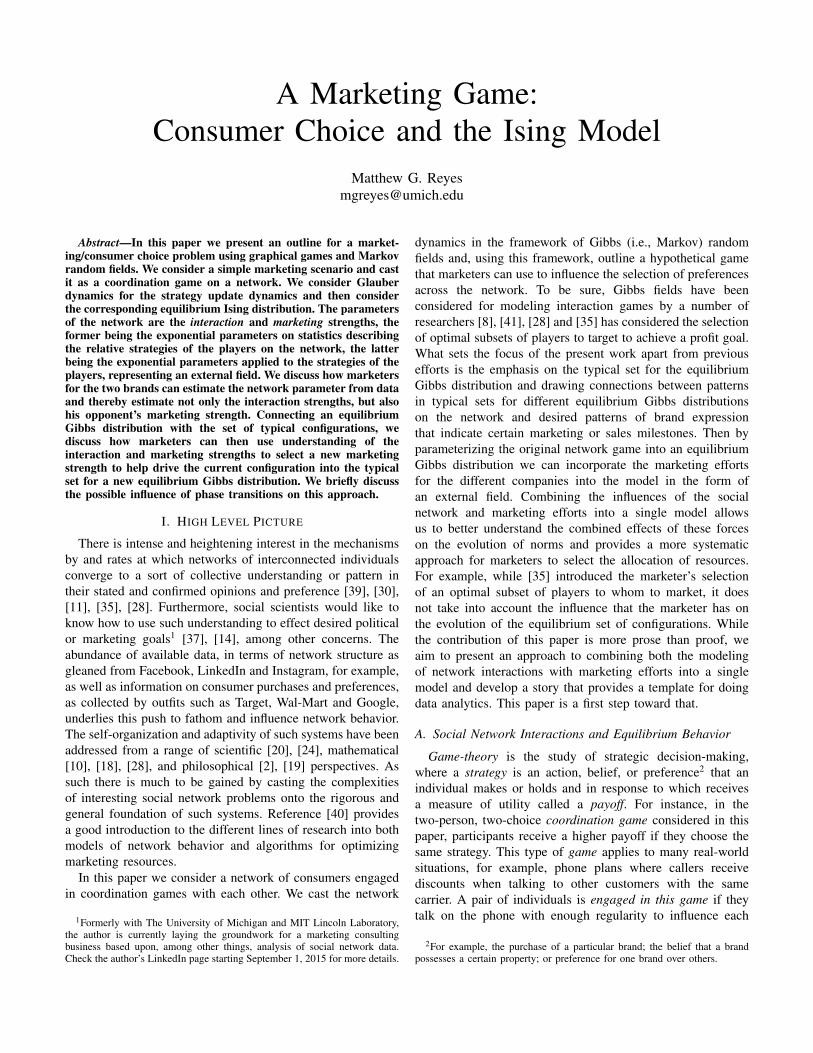
A key feature of a social network interaction that determinesthe influence of pairwise interactions on the emergence ofa global pattern in network choices is the topology of thenetwork. In other words, who’s connected to whom, wheretwo individuals are said to be connected if they are neighbors.Properties such as the number steps to go from one person tothe next, the presence of cycles and other substructures, andso on, are topological properties. Research has established thatsocial networks possess certain topological properties, suchas a degree distribution that follows a power law, termeda scale-free topology; as well as short average path lengthand high clustering coefficient [30], termed the Small Worldtopology [30]. Furthermore, it has been shown that socialnetworks consist of many small communities within which theties or connections are strong, with these small communitiesconnected through weaker ties [30], [11]. It has been arguedthat these topological properties are key in the propagation ofnorms through a social network [30], [11]. There are waysto generate both a scale-free topology, a small-world startingfrom a regular graph [30]. An example of both a 5 × 5 gridgraph and a small-world graph generated from it are shownin Figure 1 (a) and (b), respectively. For convenience, thisexamples shown in the paper will be on grid graphs.

In addition to the network topology, what determines thespread of a particular idea or preference for a particular brandare the dynamics on the network. The dynamics refer tothe influence of players’ strategies on those of other playersin the network. Two prominent types of dynamics modelsconsidered in the literature are cascade models which describeviral behavior where preferences percolate through a networkby probabilistically propagating from neighbor to neighbor[30], [26]; and local interaction game models, in whichindividuals update their preferences based on the preferencesof their neighbors and the respective games played between the

(a) (b) (c)

Fig. 1. (a) Original 5 × 5 grid graph; (b) New graph with edges re-wiredwith probability .5; and (c) A 5× 5 grid subgraph of an infinite graph.

neighbors [12], [41], [22]. Both cascade and local interactiongame models consider the time evolution of the configurationof strategies on the network. In [8], the connection is madebetween the temporal dynamics of local interaction games andGibbs distributions describing the equilibrium configurationsof strategies on the network.

There are two interesting phases to the dynamics on anetwork. The transient phase and the equilibrium phase. Withregard to the spread of a preference throughout the network,it is the transient phase that is the most interesting, in thatgives us an idea of how fast a preference will spread throughthe network before an equilibrium is reached. Considerablework has looked at the speed at which cascade models spreadthrough networks of different topologies [26], and the resultshave cast doubt [39] on the supposition that the adoptionof a brand by certain key influentials triggers a cascadeof preference for that brand. Furthermore, recent researchshows that the rates of convergence for local interaction gamemodels on various topologies are diametric to those undercascade models, suggesting that local interaction games maybe better suited to explain the spread of preference through anetwork [28]. In this paper we consider local interaction gameswith stochastic-response Glauber dynamics in which playersupdate their decisions randomly according to a probabilitydistributions that is log-linear in the payoff margins.

In this paper we are looking at the equilibrium Gibbsdistribution to which the Glauber dynamics converge. Byexpressing the payoff margin as the product of a statisticthat measures whether the strategies of two players agreeor disagree, and an exponential parameter which quantifiesthe strength of interaction between the two players, we cancast the network coordination game in the Gibbs/Glauberframework, which we will use in setting up the game thatmarketers can play, discussed in Section IV. Part of this gameinvolves estimating the interaction strengths on the network. Itis well-known that Gibbs distributions are maximum-entropydistributions over the space of strategy configurations, subjectto constraints on the expected values of the statistics. Thusone can collect data and derive a Gibbs distribution which isconsistent with the data but assumes no more about the randomevolution of the strategy configuration on the network.

An equilibrium Gibbs distribution is stationary in the sensethat, once equilibrium is reached, the distribution on the set

(a) (b) (c)

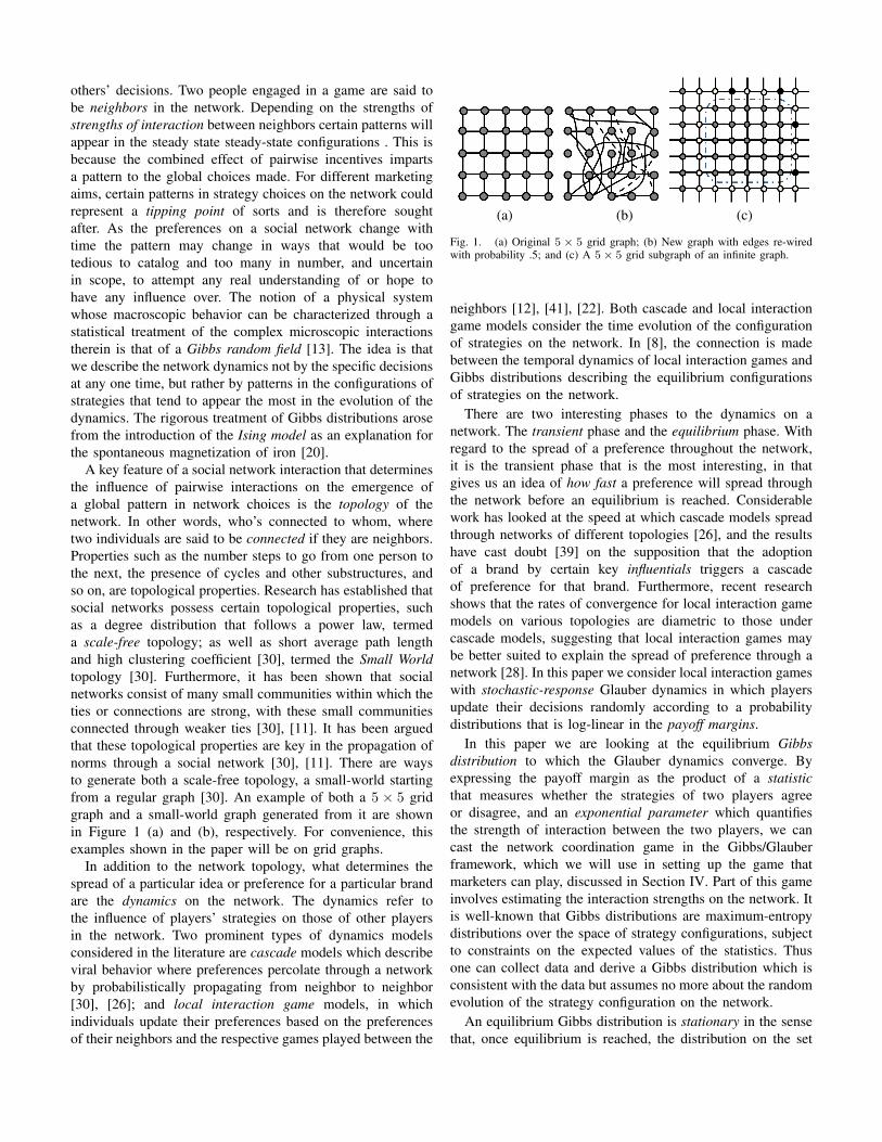
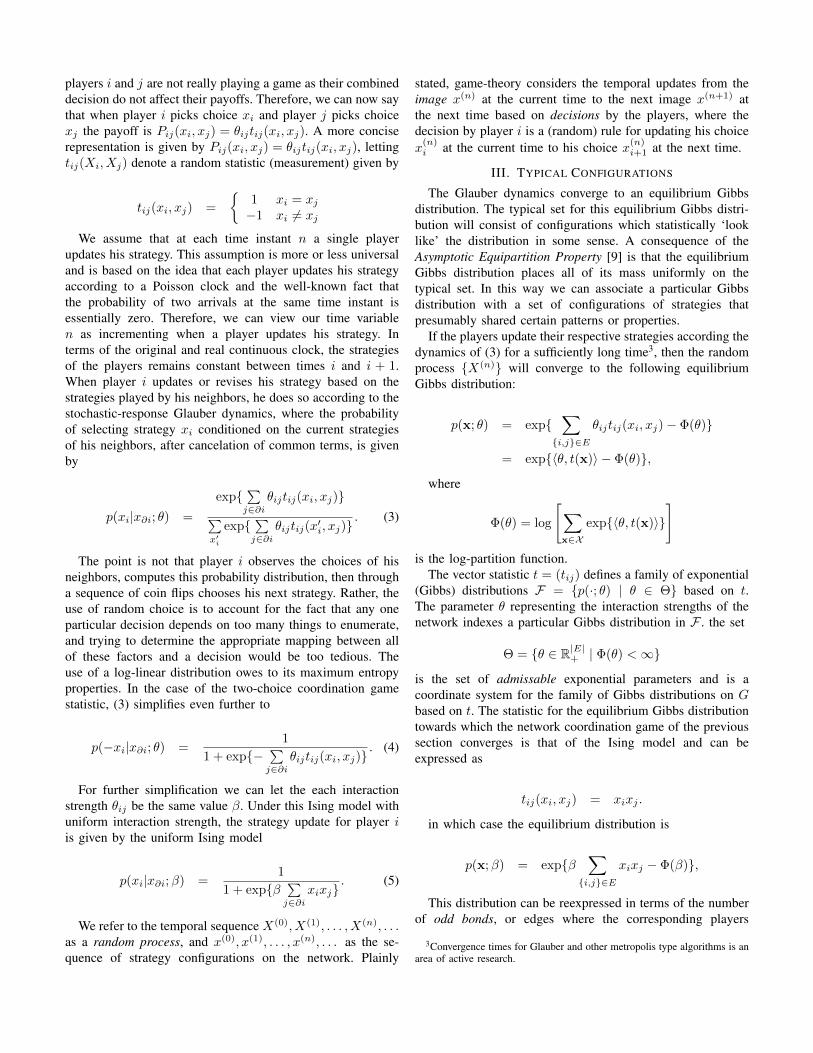
Fig. 2. Typical images from an Ising distribution on a 200× 200 4-pt. gridwith uniform interaction strength θ = (a) .4; (b) .44; and (c) .5.

of configurations is the same at each time. In general networkparameters will change with time [1]. Thus the idea presentedhere is a first step in a more complicated model where transientbehavior is accounted for. An equilibrium Gibbs distributionwill put nearly all of its mass roughly uniformly on a relativelysmall subset of configurations called the typical set [9]. InFigure 2 we can see typical images from the Ising distributions.Therefore we can associate to each set of interaction strengths,which are exponential parameters in the Gibbs distribution, aset of strategy configurations that ‘look like’ the distributionin terms of the particular statistic that represents the game. Forexample, Best-response dynamics is a limiting case of Glauberdynamics with infinite interaction strength. The typical set forthis extreme Gibbs distribution consists of the configurationwhere everyone chooses brand A and the configuration whereeveryone chooses brand B. However, Glauber dynamics ap-plied to one of these typical configurations will never reach theother typical configuration which is related to reasons givenin [28] for why Nash equilibria may not be a good way tounderstand network dynamics. This concept is related to phasetransitions in families of Gibbs distributions, will be discussedbriefly in Section V.

B. Gibbs Fields for Marketing Analytics

Beyond understanding the dynamics that contribute to thespread of preferences on a network, there is a desire to usethis understanding to promote the widespread preference for aparticular brand or idea [40], [23], [35]. This generally takesthe form of selecting which players in the network to targetwith marketing efforts. In [23], for example, cascade dynamicsare considered, while in [35] equilibrium Gibbs distributionsare considered. Thus our approach is aligned with [35] inthat we are casting it in the steady-state Gibbs frame workyet still includes the temporal dynamics through the Glauberspecification, and as such is similar to [23].

At a given time we want to select a correct group ofplayers to target with marketing efforts. In Section IV wepropose a game that marketers from competing companiescan play against each other to influence the expression ofbrand preferences on the network. To begin, add an externalfield to the Gibbs distribution to represent marketing strengthapplied to the certain players. An external biases the strategiesof the players [25]. Each of the two marketers will choosea subset of sites to apply their marketing strength upon.

The combined marketing strength at a site will be the sumof the marketing strengths for the two marketers. Where toapply marketing strength and to what extent depends on anumber of factors. For certain interaction strengths, more orless marketing strength may need to be applied to achieve adesired effect on the network. Moreover, if we could learn orestimate the marketing strength that our opponent is applying,this would also allow us to allocate marketing resources(near) optimally. Gibbs distributions are parameterized by dualcoordinate systems [3]. The first set of coordinate are theinteraction and marketing strengths. The second coordinatesystem is the set of expected statistics and expected strategieson the network. By collecting data in the form of sales infor-mation we can determine averages for the relevant statisticsand estimate the network parameters. This estimate will allowhim to make a (near) optimal choice in marketing strength thenext time.

A marketer may express his goals in terms sets of config-urations of strategies on the network that possess a desiredproperty. For instance, a uniform Ising model with a highenough interaction strength will produce typical images thathave giant monotone clusters of sites. Such clustering ofsites, interpreted in the current marketing scenario, wouldcorrespond to positive brand expression and is an exampleof a property that a marketer may seek. Each marketer couldthen define a subset of configurations that possess a favorableproperty with respect to his brand. This subset of configura-tions would then serve as a target set of configurations towardswhich they would like to drive the evolution of the typicalset for the random strategy process. If a marketer associatespatterns within typical sets of different Gibbs distributionswith such a desired set of configurations, by modifying thehis marketing strength he may be able to tip the market in hisfavor.

C. Infinite Networks and Multiple Equilibria

Though all networks are finite, it can helpful to illuminatethe behavior of a large network by considering the propertiesof an infinite network. In the case of Gibbs measures oninfinite networks, they are specified by (conditional) Gibbsdistributions on all finite subsets given all possible boundaryconfigurations. Any probability measure whose conditionalprobabilities agree with these conditional (Gibbs) distributionswill be called a Gibbs measure relative to the given specifi-cation [13]. A Gibbs measure is a macroscopic equilibriumdistribution over the set of strategies. It is sometimes thecase that there are multiple equilibrium Gibbs measures fora given specification. Each such equilibrium Gibbs measureis considered to be a distinct ‘mode’ of the random field. Aconvenient way of thinking about this is that nature choosesone of the modes at a time minus infinity, and subsequentlyeach configuration on the network is drawn from that chosenGibbs measure. We just do not know which mode was chosen.If there is only one mode for an equilibrium Gibbs distribution,then the random process that converged to that distributionis ergodic, which means empirical averages equal statistical

averages. If there are multiple modes, the dynamimcs are non-ergodic and we cannot estimate statistical probabilities fromdata [16].

For example the phenomenon of spontaneous magnetizationis an example of a phase transition. Even when there is noexternal magnetic field applied, a bar of iron will sponta-neously magnetize at a given temperature. When this happensthe distribution of atomic spins moves away from the fifty-fiftysplit and a large clustering of sites will have the same spin.We can think of this as the typical set splitting into subsetssuch that once the process is in one of the subsets of theseconfigurations, the process will not reach any of the othersubsets. In terms of the random process of evolving strategies,we say that two such typical sets do not communicate. We cansee typical images for a different values of the exponentialparameter for uniform Ising models in Figure 2. We can seethat as the exponential parameter is increased the sites becomegrouped together in larger and larger clusters, though theseclusters remain sufficiently far apart from one another. Oncethe exponential parameter reaches the critical value, solvedby Onsager in 1944, these smaller clusters merge with oneanother an form a giant cluster that extends throughout thenetwork. Essentially, the influence of the initial pattern ofstrategies in the network does not fade away and the particularequilibrium Gibbs measure observe is determined by both theinitial configuration and the Glauber dynamics that specify theGibbs measure.

The problem of multiple equilibria in networks of localinteraction games has been considered in the literature [8],[41], [12], [28]. Much analysis has centered on best-responsedynamics and associated Nash equilibria. A complaint of Nashequilibria is given in [28] because of the multiple equilibriaof the best-response dynamics. Best-response dynamics is alimiting example of Glauber dynamics in which all inter-action strengths on the network are infinite. In the absenceof an external field, best-response dynamics is non-ergodicand converging to one of multiple non-communicating anddegenerate typical sets. Our model includes marketing in theGibbs distribution so it will be interesting in the future to see ifapplying an external field influences the observed degeneracyof best-response dynamics. In either case, with regards to ourapproach, care will need to be taken in understanding theexistence of multiple ‘disjoint’ typical sets associated with agiven interaction and marketing strength, and in how to takeadvantage or or guard against any interesting consequences ofthe phase transition on the proposed game. We do not take upthis matter in the present paper, though we do introduce thenotion of a phase transition in Section V.

D. Outline of Paper

In Section II we define graphs and a network coordinationgame with Glauber dynamics. In Section III we discuss Gibbsdistributions and typical sets. In Section IV we introduce agame using an external field to represent marketing strengthand drive the typical set of an equilibrium Gibbs distributionto a new typical set possessing desired properties. In Section

V we discuss the presence of phase transitions and what thismay mean for the marketing game we have in mind, and inSection VI we discuss some experiments.

II. NETWORK COORDINATION GAME

Consider a set of sites V where a site corresponds to aperson in a social network, a network consisting of peo-ple whose neighbor relations are determined through directcontact through the telephone. We will first consider thecase where V is finite, the case where V is infinite willbe considered in Section V. A set of edges E consists ofpairs of adjacent players i and j, regarded as neighbors. Theobject G = (V,E) is a graph with sites or players V andundirected edges E. For each site i ∈ V , Ωi is the finitealphabet or strategy space for player i. Here, the strategyspace is the same Ωi = Ω = −1, 1 for all players i ∈ V .For concreteness, think of two phone carriers, the two valuesin Ω corresponding to the two carriers. Let xi = −1 indicatethat player i prefers or is a customer of the brand assigned −1,and likewise if xi = 1. Time will be taken to be discrete andwill be denoted by n, taking values in the sequence of non-negative integers 0, 1 . . . , n, . . .. For i ∈ V , X(n)

i denotesthe random strategy of player i, where x

(n)i is the actual

value assumed at time n. At time n, the collection of randomvariables X(n) = X(n)

i is a random field and x(n) = x(n)i

is the image or configuration on the network at time n.For i, j ∈ E, players i and j are engaged in a two-choice

coordination game. The payoff matrix for this game is Pij andis denoted by

Pij =

[aij bijbij aij

], (1)

where aij > bij indicates a higher payoff when the playersagree versus disagree. In this case Pij(xi, xj) indicates thepayoff when player i plays strategy xi and player j playsstrategy xj .

Consider the symmetric coordination game being playedbetween all pairs of nodes i and j, with i, j ∈ E. Foreach edge i, j ∈ E, the payoff matrix Pij from (1) canbe rewritten as

Pij =

[aij+bij

2 +aij−bij

2aij+bij

2 − aij−bij2

aij+bij2 − aij−bij

2aij+bij

2 +aij−bij

2

]

= pij +

[aij−bij

2 −aij−bij2

−aij−bij2aij−bij

2

]

= pij +

[θij −θij−θij θij

], (2)

Since a term of the payoff, pij , is constant over all imageson V , we can ignore it, since the interaction between playersi and j is in the margin between a guaranteed payoff and themaximum payoff. This is easy to see by considering the casethat a = b. Regardless of how large the value is, if the payoff isthe same no matter what strategies are played by i and j, then

players i and j are not really playing a game as their combineddecision do not affect their payoffs. Therefore, we can now saythat when player i picks choice xi and player j picks choicexj the payoff is Pij(xi, xj) = θijtij(xi, xj). A more conciserepresentation is given by Pij(xi, xj) = θijtij(xi, xj), lettingtij(Xi, Xj) denote a random statistic (measurement) given by

tij(xi, xj) =

1 xi = xj−1 xi 6= xj

We assume that at each time instant n a single playerupdates his strategy. This assumption is more or less universaland is based on the idea that each player updates his strategyaccording to a Poisson clock and the well-known fact thatthe probability of two arrivals at the same time instant isessentially zero. Therefore, we can view our time variablen as incrementing when a player updates his strategy. Interms of the original and real continuous clock, the strategiesof the players remains constant between times i and i + 1.When player i updates or revises his strategy based on thestrategies played by his neighbors, he does so according to thestochastic-response Glauber dynamics, where the probabilityof selecting strategy xi conditioned on the current strategiesof his neighbors, after cancelation of common terms, is givenby

p(xi|x∂i; θ) =

exp∑j∈∂i

θijtij(xi, xj)∑x′i

exp∑j∈∂i

θijtij(x′i, xj). (3)

The point is not that player i observes the choices of hisneighbors, computes this probability distribution, then througha sequence of coin flips chooses his next strategy. Rather, theuse of random choice is to account for the fact that any oneparticular decision depends on too many things to enumerate,and trying to determine the appropriate mapping between allof these factors and a decision would be too tedious. Theuse of a log-linear distribution owes to its maximum entropyproperties. In the case of the two-choice coordination gamestatistic, (3) simplifies even further to

p(−xi|x∂i; θ) =1

1 + exp−∑j∈∂i

θijtij(xi, xj). (4)

For further simplification we can let the each interactionstrength θij be the same value β. Under this Ising model withuniform interaction strength, the strategy update for player iis given by the uniform Ising model

p(xi|x∂i;β) =1

1 + expβ∑j∈∂i

xixj. (5)

We refer to the temporal sequence X(0), X(1), . . . , X(n), . . .as a random process, and x(0), x(1), . . . , x(n), . . . as the se-quence of strategy configurations on the network. Plainly

stated, game-theory considers the temporal updates from theimage x(n) at the current time to the next image x(n+1) atthe next time based on decisions by the players, where thedecision by player i is a (random) rule for updating his choicex

(n)i at the current time to his choice x(n)

i+1 at the next time.

III. TYPICAL CONFIGURATIONS

The Glauber dynamics converge to an equilibrium Gibbsdistribution. The typical set for this equilibrium Gibbs distri-bution will consist of configurations which statistically ‘looklike’ the distribution in some sense. A consequence of theAsymptotic Equipartition Property [9] is that the equilibriumGibbs distribution places all of its mass uniformly on thetypical set. In this way we can associate a particular Gibbsdistribution with a set of configurations of strategies thatpresumably shared certain patterns or properties.

If the players update their respective strategies according thedynamics of (3) for a sufficiently long time3, then the randomprocess X(n) will converge to the following equilibriumGibbs distribution:

p(x; θ) = exp∑i,j∈E

θijtij(xi, xj)− Φ(θ)

= exp〈θ, t(x)〉 − Φ(θ),

where

Φ(θ) = log

[∑x∈X

exp〈θ, t(x)〉

]is the log-partition function.

The vector statistic t = (tij) defines a family of exponential(Gibbs) distributions F = p(·; θ) | θ ∈ Θ based on t.The parameter θ representing the interaction strengths of thenetwork indexes a particular Gibbs distribution in F . the set

Θ = θ ∈ R|E|+ | Φ(θ) <∞

is the set of admissable exponential parameters and is acoordinate system for the family of Gibbs distributions on Gbased on t. The statistic for the equilibrium Gibbs distributiontowards which the network coordination game of the previoussection converges is that of the Ising model and can beexpressed as

tij(xi, xj) = xixj .

in which case the equilibrium distribution is

p(x;β) = expβ∑i,j∈E

xixj − Φ(β),

This distribution can be reexpressed in terms of the numberof odd bonds, or edges where the corresponding players

3Convergence times for Glauber and other metropolis type algorithms is anarea of active research.

disagree in their strategy. When the interaction strengths arenot uniform, odd and even bonds are weighted according tothe respective interaction strengths. For a stationary (equi-librium) distribution over the set of possible configurationsof strategies on a finite network, the equilibrium distributionactually places its mass roughly uniformly on a relativelysmall subset of configurations called the typical set. There aremultiple definitions of typicality. For example, weak or entropytypicality of a configuration is satisfied if the probability ofthe configuration under the stationary distribution is roughly2 to the negative logarithm of the entropy of the process, i.e..We denote the typical set as ΩT (θ). Typical configurationsfor the Ising model, and thus the network coordination gamethat it models can then be classified according to the numbersof odd bonds they possess. In this way it makes sense tothink of configurations ‘looking like’ a particular distributionor interaction strength. In Figure 2 we see typical image fromdifferent uniform interaction strength Ising models.

Moreover, the statistic for the Ising model has the propertythat for positive exponential parameters, any two componentsof the statistic tij and tkl have positive covariance. This wasshown by Griffiths [17] in the case of the Ising model. In [31],we termed this property positive correlation and have showed[31], [32], [33] that families of Gibbs distributions defined bya statistic having this property have certain monotonicity prop-erties. Looking at coordination game dynamics as a stochastic-response with interaction strength θ, it is clear that best-response dynamics that tend towards Nash equilibria is thelimiting case where θ =∞. The limiting assumption of best-response dynamics, then, may be appropriate for the dynamicswithin smaller communities, though when considering tiesbetween these small communities, it is likely too extreme.Conclusions from [28] make a compelling argument againstNash equilibria because the different equilibria are ratherdiverse. We believe that looking at a local interaction gameon a network in the Gibbs/Glauber framework permits focusnot on the extreme. This makes sense, because as θ → ∞,the mass of the equilibrium Gibbs distribution is on the all‘-1’s configuration and the all ‘+1’s configuration. Thus theconfigurations one would expect to be ‘drawn from’ thisdistribution will be close to a uniform configuration. That suchconfigurations are so diverse is explored later in Section V.As actual social networks consist of many small communitiesconnected by ‘strong ties’, with these small communitiesconnected to each other through ‘weak ties’, best-responsedynamics may be appropriate on small subsets of nodes but onthe larger scale, general Glauber dynamics is more compelling.

IV. MARKETING GAME:DRIVING THE EVOLUTION OF THE TYPICAL SET

In this section we introduce a game that two opposingmarketers, A and B, can engage in to influence brand ex-pression on the network. The version of the game that wepresent here is a simplified version of a more complicatedgame that can be played. Marketers A and B will applyexternal fields to select players in the network. The external

field represents marketing strength that influences the strategyupdate dynamics in addition to the interaction strengths thatrepresent the influence due to social affiliations. To do this weintroduce an identity statistic ti(·) for each player. Moreover,we look at the exponential parameter θ as now consistingof a portion θE corresponding to interaction strengths, anda portion θV corresponding to marketing strengths. The in-teraction strengths θE are assumed to be constant, but themarketing strengths θ(n)

V will be updated by marketers A andB and will thus be superscripted as such. The marketingstrength from player A at time n is denoted ψ

(n)V |A, and

likewise for player B and ψ(n)V |B . The total marketing strength

is θ(n)V = ψ

(n)V |A + ψ

(n)V |B . Without loss of generality we let

θA ≺ 0 and θB 0. Thus the marketing strength ψ(n)V |A

biases the strategies of the players to -1, whereas ψ(n)V |B biases

the strategies of the players to 1. When displaying updateequations for the players we will omit the time index forconvenience.

The Glauber dynamics for this situation are now

p(−xi|x∂i; θ) =1

1 + expθixi) +∑j∈∂i

θijxixj,

where we can think of θi has the payoff (cost) for agreeing(disagreeing) with the external field. These dynamics willconverge to the equilibrium distribution given by

p(x; θ) = exp∑i∈V

θixi +∑i,j∈E

θij ixj − Φ(θ),

and configurations will be typical for these interaction andmarketing strengths.

We assume that at time 0, the random process givenby the Glauber dynamics has converged to its equilib-rium distribution. As the sequence of network configurationsx(0), x(1), . . . , x(n−1) evolves marketers A and B collect acorresponding sequence of data x(0), x(1), . . . , x(n−1). The xare in general noisy versions of the true x. Noise could repre-sent missed collects due to limited resources, or corruption ofsignal due to channel error. Here we will consider the noiselesscase. While in general we would want to distinguish betweenx collected by marketer A versus x collected by marketer B,we will not do so here for simplicity. The data of interest is thesequence of statistics t(0) = t(x(0)), t(1) = t(x(1)), . . . , t(1) =t(x(n−1)). From this we compute the statistic

t(n) =1

n

m−1∑i=0

t(x(n−i)).

From this information the marketers would like to estimateθ(n), from which they have an estimate of the interactionstrengths θ(n)

E . This would also give them an estimate of themarketing strengths θ(n)

V . And since they know the value ofψV |A (ψV |B), they could estimate ψV |B (ψV |A).

(a) (b) (c)

(d) (e) (f)

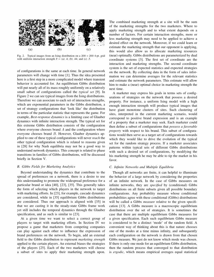
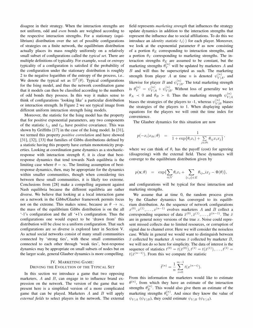
Fig. 3. Typical images from an Ising distribution on a 200 × 200 4-pt.grid with uniform interaction strength β = (a) .2; (b) .3; and (c) .4, and zeroexternal field; and with uniform interaction strength and marketing strengthα = .05 in (d), (e), and (f).

A. Parameter Estimation

For each θ ∈ Θ, the expected value of the statistic t is thevector Eθ [t] = µ, which is referred to as the moments of theMRF under θ. The set of all moments corresponding to MRFsbased on t is

M = µ ∈ R|E| | ∃θ ∈ Θ,Eθ[t] = µ.

If the components of t are affinely independent, the statisticis said to provide a minimal representation of F . In this case,it is well-known that the mapping p : Θ −→ F is one-to-one, in which case F is a statistical manifold with dualcoordinate systems Θ and M [3], [4]. This dual coordinatesystem provides, among other things, a method for estimatingthe exponential parameters from measured averages collectedfrom typical configurations. There are well-known algorithmsfor performing (approximating) these algorithms, dependingas it were on the topology of the network [3], [38].

We let θ|A(t(n)) be the parameter estimator for marketerA and likewise for θ|B(t(n)) and marketer B. Marketer Aforms the estimate θ(n)

|A = θ|A(t(n)) from the measurementst(n) of the configurations x(n−m+1), x(n−m+2), . . . , x(n). Hethen forms the estimate of θ(n) given the data and estimationalgorithm of marketer A and from this estimate of the totalinteraction and marketing strength, form an estimate

ψ(n)V |B = θ

(n)|A − ψ

(n)V |A

of his opponent’s marketing strength. Likewise, marketer Bestimates θ(n)

|B with his estimation algorithm, and from this

derives an estimate ψ(n)V |A. Since he knows ψ(n)

V |B , he under-stands not only the interaction strengths of the network, butwhere he and his opponent are investing their resources.

B. Desired Configurations

The idea is to connect this desired set of images with typicalsets for different values of the of the exponential parametersor interaction strengths. Then, we can look at subspaces of theparameter set Θ as indexing sets of configurations with certainstatistical properties and patterns. By finding a correspondencebetween the patterns of images in different typical sets andthe desired patterns for the expression of a particular brand,one can use knowledge of the interaction strengths to decidehow much marketing strength to apply in order to drive thecurrent typical set to a desired typical set. For example, inIsing models with no external field, there is a certain value,called the critical value, such that typical images containa ‘giant cluster’ of sites having the same strategy. Thus adesired set of configurations could defined in terms of a largemonotone cluster having some geometric properties of theimage representing significant representation on the network,for example. Then by drawing a connection between thisdesired set of patterns and the patterns depicted in typicalsets for different Gibbs distributions, we can identify possibleplaces where the addition of marketing strength could drivethe Glauber dynamics into a new typical expressing desiredproperties.

For instance, marketer A can define his set Ω∗A of desiredconfigurations as

Ω∗A =⋃

θ′∈ΘA

ΩT (θ′)

where

ΘA = θ ∈ Θ : ΩT (θ) ⊂ Ω∗A

is the set of interaction and marketing strengths such that theset of configurations with desired property for A contains thetypical set for these interaction and marketing strengths. This isjust an example of how one might relate elements to ΩT (θ) :θ ∈ Θ. An alternative definition of ΘA could be

ΘA = θ ∈ Θ : ΩT (θ) ⊃ Ω∗A

.In addition to considering containment based relationships,

we could define relationships based on proximity in somesense. For some distance function d : Ω × Ω −→ R+ onthe product space of configurations on the network, we coulduse

d(ΩT (θ),Ω∗A

)< ρ

as the membership criterion. The point is by connectingexponential parameters to typical sets of configurations thatare likely to possess desired properties, we can adjust themarketing strength applied in different regions.

C. Playing a Marketing Strength

With estimates θ(n)|A and θ(n)

|B and with recent data collects,marketers A and B now update their own strategies, which

are their respective marketing strengths. We assume that thedesired sets of configurations Ω∗A and Ω∗B are constant forthe entire game. Marketers A and B updating their marketingstrengths to ψ

(n+1)V |A and ψ

(n+1)V |B , respectively. At time n,

marketer A will chooses to ‘play’ marketing strength ψ(n)V |A,

and likewise, marketer B plays ψ(n)V |B . At the next time instant

n+1 players A and B choose new marketing strengths ψ(n+1)V |A

and ψ(n+1)V |B according to some functions

ψ(n+1)V |A = F

(x(n(m)), θ

(n)E|A, ψ

(n)V |B , ψ

(n)V |A,Ω

∗A

)and

ψ(n+1)V |A = F

(x(n(m)), θ

(n)E|B , ψ

(n)V |A, ψ

(n)V |B ,Ω

∗B

)that takes into account the most recent block of configurations,the estimated interaction strengths, the estimated marketingstrength for his opponent, and his known marketing strength.These functions may also depend on the respective desiredsets of configurations Ω∗A and Ω∗B .

If x(n) ∈ Ω∗A, then marketer can seek to buttress hisadvantage through appropriately updating (or maintaining) hismarketing strength. This may be accomplished, for instance,by moving the typical set ‘deeper into‘ the desired set Ω∗A. Ifx(n) 6∈ Ω∗A marketer A wants to choose a marketing strengthψ

(n+1)V |A that drives the typical set toward Ω∗A. For example,

marketer A may choose the target Gibbs distribution, i.e. thenext typical set, with a criterion such as

minθ′:(θ′)E=θE

maxx′∈ΩT (θ)

d(x(n), x′)

for some appropriately defined distance measure, for examplethe Earth Mover’s Distance [36]. In setting, though we do nothave in mind a database of images with which to compare thecurrent configuration x(n), but rather a way to determine fromx(n) how far it is from possessing the respective patterns ofdifferent typical sets.

V. PHASE TRANSITIONS AND ERGODIC COMPONENTS

Let V be infinite, for instance the sites being the set ofordered pairs of natural numbers, and again let E consist of allpairs of horizontally and vertically adjacent sites. Furthermore,let the players on the infinite network G = (V,E) updatetheir strategies according to the Glauber dynamics of (3) and(5). Let L be the set of all finite subsets of V . For Λ ∈ Land boundary configuration x∂Λ, the random process (X

(n)Λ )

converges to the (conditional) Gibbs distribution

p(xΛ|x∂Λ; θ) =expΨΛ(xΛ) + ΨΛ|∂Λ(xΛ, x∂Λ)

ZΛ|∂Λ(θ)

(6)

where ΨΛ(x) = 〈sΛ, tΛ(xΛ)〉 and ΨΛ|∂Λ(x) =〈sΛ,∂Λ, tΛ,∂Λ(xΛ, x∂Λ)〉.

Moreover,

(a) (b) (c)

(d) (e) (f)

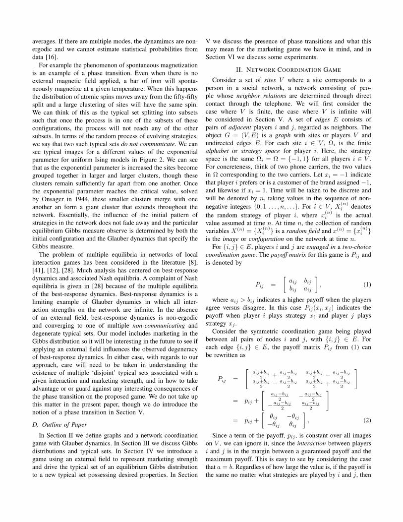
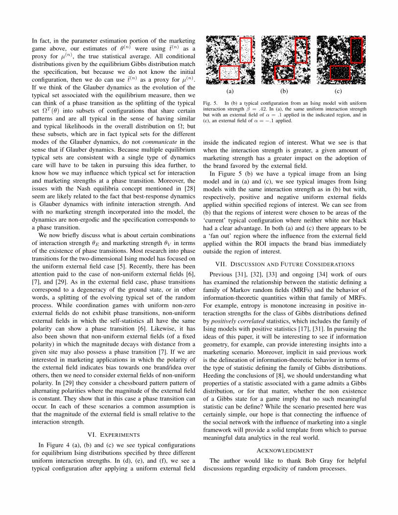
Fig. 4. In (a), (b), and (c) typical configurations from Ising models withuniform interaction strength β = .3, .4, and .5, respectively; In (d), (e), and(f), typical configurations from Ising models with the same uniform interactionstrengths as in (a), (b), and (c), but with a uniform external field of α = .05applied.

ZΛ|∂Λ(θ) =∑

xΛ∈ΩΛ

expΨΛ(x) + ΨΛ|∂Λ(x)

is the conditional partition function on Λ given the boundaryconfiguration xΛ. Likewise, the set

ΘΛ|∂Λ = s ∈ R|E|+ | ΦΛ|∂Λ(θ) <∞

is the set of admissable interaction strengths in Λ withboundary configuration x∂Λ, while FΛ|∂Λ = p(·; θ) | θ ∈ΘΛ|∂Λ is the family of conditional Gibbs distributions on Λwith boundary configuration x∂Λ, based on t. The collectionpΛ|∂Λ : Λ ∈ L of these conditional Gibbs distributions iscalled a specification, specifically a Gibbsian specification, inthat they specify the dependence type for a probability measureon the infinite random field Xi : i ∈ V . A probabilitymeasure on Xi : i ∈ V that agrees with the specificationpΛ|∂Λ : Λ ∈ L is called a Gibbs measure relative to thespecification [13]. Let G(θ, t) be the set of Gibbs measuresrelative to the specification given by the payoffs θ and thestatistic t. If |G(θ, t)| = 1 the Glauber dynamics are ergodic,while if |G(θ, t)| > 1, the dynamics are non-ergodic anda phase transition is said to occur. The equilibrium Gibbsmeasure is a discrete stationary random process and as suchis a mixture of stationary ergodic random processes [16], witheach mode of the process being a stationary ergodic process.This is referred to as the Ergodic Decomposition of discretestationary random processes [15], and we can think of thisdecomposition as being a decomposition of the space Ω of allstrategy configurations into subsets of configurations which aretypical sets for the different modes of the Glauber dynamics.

The presence of a phase transition will affect a marketer’sability to estimate θ(n) from data. If If |G(θ, t)| = 1 dynamicsare ergodic and sample averages t(n) equal statistical averages.

In fact, in the parameter estimation portion of the marketinggame above, our estimates of θ(n) were using t(n) as aproxy for µ(n), the true statistical average. All conditionaldistributions given by the equilibrium Gibbs distribution matchthe specification, but because we do not know the initialconfiguration, then we do can use t(n) as a proxy for µ(n).If we think of the Glauber dynamics as the evolution of thetypical set associated with the equilibrium measure, then wecan think of a phase transition as the splitting of the typicalset ΩT (θ) into subsets of configurations that share certainpatterns and are all typical in the sense of having similarand typical likelihoods in the overall distribution on Ω; butthese subsets, which are in fact typical sets for the differentmodes of the Glauber dynamics, do not communicate in thesense that if Glauber dynamics. Because multiple equilibriumtypical sets are consistent with a single type of dynamicscare will have to be taken in pursuing this idea further, toknow how we may influence which typical set for interactionand marketing strengths at a phase transition. Moreover, theissues with the Nash equilibria concept mentioned in [28]seem are likely related to the fact that best-response dynamicsis Glauber dynamics with infinite interaction strength. Andwith no marketing strength incorporated into the model, thedynamics are non-ergodic and the specification corresponds toa phase transition.

We now briefly discuss what is about certain combinationsof interaction strength θE and marketing strength θV in termsof the existence of phase transitions. Most research into phasetransitions for the two-dimensional Ising model has focused onthe uniform external field case [5]. Recently, there has beenattention paid to the case of non-uniform external fields [6],[7], and [29]. As in the external field case, phase transitionscorrespond to a degeneracy of the ground state, or in otherwords, a splitting of the evolving typical set of the randomprocess. While coordination games with uniform non-zeroexternal fields do not exhibit phase transitions, non-uniformexternal fields in which the self-statistics all have the samepolarity can show a phase transition [6]. Likewise, it hasalso been shown that non-uniform external fields (of a fixedpolarity) in which the magnitude decays with distance from agiven site may also possess a phase transition [7]. If we areinterested in marketing applications in which the polarity ofthe external field indicates bias towards one brand/idea overothers, then we need to consider external fields of non-uniformpolarity. In [29] they consider a chessboard pattern pattern ofalternating polarities where the magnitude of the external fieldis constant. They show that in this case a phase transition canoccur. In each of these scenarios a common assumption isthat the magnitude of the external field is small relative to theinteraction strength.

VI. EXPERIMENTS

In Figure 4 (a), (b) and (c) we see typical configurationsfor equilibrium Ising distributions specified by three differentuniform interaction strengths. In (d), (e), and (f), we see atypical configuration after applying a uniform external field

(a) (b) (c)

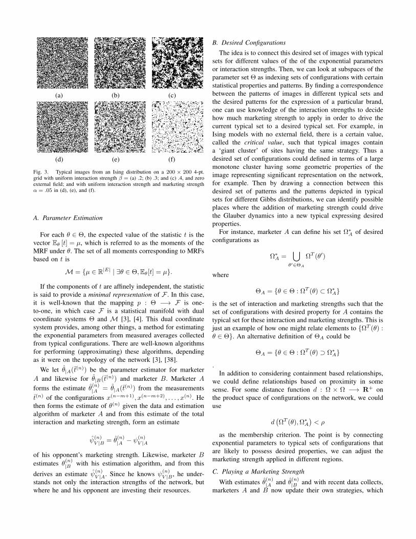
Fig. 5. In (b) a typical configuration from an Ising model with uniforminteraction strength β = .42. In (a), the same uniform interaction strengthbut with an external field of α = .1 applied in the indicated region, and in(c), an external field of α = −.1 applied.

inside the indicated region of interest. What we see is thatwhen the interaction strength is greater, a given amount ofmarketing strength has a greater impact on the adoption ofthe brand favored by the external field.

In Figure 5 (b) we have a typical image from an Isingmodel and in (a) and (c), we see typical images from Isingmodels with the same interaction strength as in (b) but with,respectively, positive and negative uniform external fieldsapplied within specified regions of interest. We can see from(b) that the regions of interest were chosen to be areas of the‘current’ typical configuration where neither white nor blackhad a clear advantage. In both (a) and (c) there appears to bea ‘fan out’ region where the influence from the external fieldapplied within the ROI impacts the brand bias immediatelyoutside the region of interest.

VII. DISCUSSION AND FUTURE CONSIDERATIONS

Previous [31], [32], [33] and ongoing [34] work of ourshas examined the relationship between the statistic defining afamily of Markov random fields (MRFs) and the behavior ofinformation-theoretic quantities within that family of MRFs.For example, entropy is monotone increasing in positive in-teraction strengths for the class of Gibbs distributions definedby positively correlated statistics, which includes the family ofIsing models with positive statistics [17], [31]. In pursuing theideas of this paper, it will be interesting to see if informationgeometry, for example, can provide interesting insights into amarketing scenario. Moreover, implicit in said previous workis the delineation of information-theoretic behavior in terms ofthe type of statistic defining the family of Gibbs distributions.Heeding the conclusions of [8], we should understanding whatproperties of a statistic associated with a game admits a Gibbsdistribution, or for that matter, whether the non existenceof a Gibbs state for a game imply that no such meaningfulstatistic can be define? While the scenario presented here wascertainly simple, our hope is that connecting the influence ofthe social network with the influence of marketing into a singleframework will provide a solid template from which to pursuemeaningful data analytics in the real world.

ACKNOWLEDGMENT

The author would like to thank Bob Gray for helpfuldiscussions regarding ergodicity of random processes.

REFERENCES

[1] A. Ahmed and E.P. Xing, “Recovering time-varying networks of depen-dencies in social and biological studies,” PNAS, July 21, 2009, vol. 106,no. 29.

[2] W.R. Ashby, “Principles of the Self-organizing System,”, Principles ofSelf-Organization: Transactions of the University of Illinois Symposium,1962, Pergamon Press: London, UK, pp. 255-278.

[3] S. Amari and H. Nagaoka, Methods of Information Geometry, OxfordUniversity Press, 2000.

[4] O.E. Barndorff-Nielson, Information and Exponential Families, Chich-ester, U.K.: Wiley, 1978.

[5] R.J. Baxter, Exactly Solved Models in Statistical Mechanics, New York:Academic, 1982.

[6] R. Bissacot and L. Cioletti, Phase Transition in Ferromagnetic IsingModels with Non-Uniform External Magnetic Fields, March 2010, arXiv.

[7] R. Bissacot, M. Cassandro, L. Cioletti, and E. Presutti, Phase Transitionsin Ferromagnetic Ising Models with spatially dependent magnetic fields,Aug. 2014, arXiv.

[8] L.E. Blume, The Statistical Mechanics of Strategic Interaction, Gamesand Economic Behavior, 5, pp. 387-424 (1993).

[9] T. Cover and J. Thomas, Elements of Information Theory, Wiley, 2005.[10] R.L. Dobrushin, “Gibbsian Random Fields For Lattice Systems with

Pairwise Interactions,” Academy of Sciences of the USSR, Translatedfrom Funktsional’nyi Analiz i Ego Prilozheniya, Vol. 2, No. 4, pp. 31-43, October-December 1968.

[11] D. Easly and J. Kleinberg, Neworks, Crowds, and Markets: ReasoningAbout a Highly Connected World, Cambridge University Press, 2010.

[12] G. Ellison, Learning, Local Interaction, and Coordination, Economet-rica, September 1993, vol. 61, no. 5.

[13] H.O. Georgii, “Gibbs Measures and Phase Transitions,” De Gruyter,New York, 1988.

[14] M. Gladwell, The Tipping Point, published by Little, Brown, andCompany.

[15] R.M. Gray and L.D. Davisson, “The Ergodic Decomposition of Sta-tionary Discrete Random Processes,” IEEE Transactions on InformationTheory, vol. IT-20, No. 5, September 1974.

[16] R.M. Gray, “Probability, Random Processes, and Ergodic Properties,”Springer-Verlag 2009.

[17] R.B. Griffiths, “Correlations in Ising Ferromagnets I.”, Jrnl. MathPhysics, 8 (478), 1967.

[18] G.R. Grimmett, “A Theorem About Random Fields,”, Bull. LondonMathematical Society, 5, 1973, pp. 81-84.

[19] F. Heylighen, “The Science of Self-Organization and Adaptivity,” FreeUniversity of Brussels, Belgium.

[20] E. Ising, “Beitrag sur Theorie des Ferromagnetismus”, Zeit. fur Physik,31 (253-258), 1925.

[21] E.T. Jaynes, Information Theory and Statistical Mechanics, The PhysicalReview, Vol 106, No 4, 620-630, May 1957.

[22] M. Kandori, H. Mailath, and F. Rob, Learning, mutation, and long runequilibria in games, Econometrica, 61:29-56.

[23] D. Kempe, J. Kleinberg, and E. Tardos, Maximizing the spread ofinfluence in a social network, Proceedings of the Ninth ACM SIGKDDInternational Confeence on Knowledge Discovery and Data Mining(KDD), 2003.

[24] R. Kikuchi, A Theory of Cooperative Phenomena, Physical Review, Vol.51, No. 6, 1950.

[25] R. Kinderman and J. Snell, Markov random fields and their applications,American Mathematical Society, vol. 1, 1980.

[26] J. Kleinberg, Cascading behavior in networks: Algorithmic and eco-nomic issues, Algorithmic Game Theory, eds N Nisan et al. (CambridgeUniversity Press, Cambridge, MA).

[27] P.V. Martin, J.A. Bonachela, and M.A. Munoz, Quenched disorderforbids discontinuous transitions in non-equilibrium low-dimensionalsystems, February 2014.

[28] A. Montanari and A. Saberi, ”The spread of innovations in socialnetworks,” PNAS, Nov. 2010.

[29] M.G. Navarrete, E. Pechersky, and A. Yambartsev, Phase transition inferromagnetic Ising model with a cell-board external field, November2014.

[30] M. Newman, A-L Barabasi, and D. J. Watts, The Structure and Dynamicsof Networks, The Princeton University Press, 2006.

[31] M. G. Reyes and D. L. Neuhoff, “Entropy Bounds for a Markov RandomSubfield,” ISIT 2009, Seoul, South Korea, July 2009.

[32] M. G. Reyes, ”Cutset processing and compression of Markov randomfields,” phd dissertation, University of Michigan, 2011.

[33] M. G. Reyes, “Covariance and Entropy in Markov Random Fields,” ITA2013, San Diego, Feb. 2013.

[34] M.G. Reyes and D.L. Neuhoff, “Monotonicity and Reduction in MarkovRandom Fields,” in preparation.

[35] M. Richardson and P. Domingos, Mining Knowledge-Sharing Sites forViral Marketing, Eigth Intl. Conf. on Knowledge Discovery and DataMining, 2002.

[36] Y. Rubner, C. Tomasi, and L. J. Guibas, A Metric for Distributions withApplications to Image Databases, Proceedings ICVV 1998: 59-66.

[37] T. Schelling, Micromotives and Macrobehavior, Norton 1978.[38] M. J. Wainwright and M. I. Jordan, Graphical models, exponential

families and variational inference, Technical Report 649, Sept. 2003.[39] D. Watss, Challenging the Influentials Hypothesis, Measuring Word of

Mouth, 3 pp:201-211.[40] J. Wortman, Viral Marketing and the Diffusion of Trends on Social

Networks, Technical Report MS-CIS-08-19, Department of ComputerScience, University of Pennsylvania, May 15, 2008.

[41] H. Peyton Young, The Evolution of Convention, Econometrica, Vol. 61,No. 1, Jan. 1993, pp. 57-84.