A Markov-Switching model of Taka/Rupee exchange rate: estimation and forecasting Raisa Shafiquddin Thesis Supervisor Dr. Syed Abul Basher A thesis presented for the degree of Masters of Social Science Department of Economics East West University Bangladesh 2016
Transcript
A Markov-Switching model of Taka/Rupee
exchange rate: estimation and forecasting
Raisa Shafiquddin
Thesis Supervisor Dr. Syed Abul Basher
A thesis presented for the degree of
Masters of Social Science
Department of Economics
East West University
Bangladesh
2016
Acknowledgement
I am thankful to almighty Allah for being merciful and gracious towards my endeavors. I am
eternally thankful to my loving parents and all my teachers, here at East West University and
elsewhere, who have been sources of immense inspiration and support all throughout my
academic journey. A special thanks to my thesis supervisor, Dr. Syed Abul Basher for giving
me the opportunity to explore the complex and intricate world of exchange rate economics.
This would not have been possible without his guidance and thorough supervision. Without
further ado, here I begin.
Copyright Statement
Student’s Permission
I hereby grant to East West University or its agents the right to archive and to make
available my Master’s thesis in all forms of media, now or hereafter known. I retain all
proprietary rights, such as patent rights. I also retain the right to use in future works
(such as articles or books) all or part of this thesis.
Name: Raisa Shafiquddin
Date:
Signature:
Supervisor’s Permission
I hereby grant to East West University or its agents the right to archive and to make
available the Master’s thesis of my student Raisa Shafiquddin, in all form of media,
now or hereafter known.
Raisa Shafiquddin retains all proprietary rights, such as patent rights and also retains
the right to use in future works (such as articles or books) all or part of this Master’s
Thesis.
Name: Dr. Syed Abul Basher
Date:
Signature:
Approval
Name: Raisa Shafiquddin
Degree: Master of Social Sciences in Economics
Title: A Markov switching model of Taka/Rupee exchange rate: estimation and forecasting
Examining Committee:
Dr. Syed Abul Basher
Thesis Supervisor
Chairperson, Department of Economics
Dr. A.K. Enamul Haque
Professor, Department of
Economics
Date Approved:
Thesis title: A Markov switching model of taka/rupee exchange rate: estimation and forecasting
Abstract: This study considers the validity of a (modified) monetary exchange rate model
between monthly Bangladeshi Taka and Indian Rupee exchange rate in a Markov-switching
framework. To reflect the beginning of the floating exchange rate regime by Bangladesh Bank,
the sample period spans from May 2003 to March 2016. Empirical results lend support for
Markov-switching model in capturing the long swings in the observed exchange rate. The
results also show that various monetary fundamentals (i.e., interest rate differential, inflation
rate differential, money growth differential, and trade balance) are statistically significant
determinants of Taka-Rupee exchange rate. It then conducts several out-of-sample forecasting
performances of the Markov-switching monetary model against a random walk model. A
rolling window Markov-switching model generates better forecasts than a random walk.
Policy implications of the results are also discussed.
Table of Contents 1. Introduction ......................................................................................................................................... 11
2. Literature Review ................................................................................................................................ 15
2.1 Structural models of exchange rate determination ................................................................... 15
2.2 Non-linear modeling of exchange rate and fundamentals ....................................................... 17
2.3 Developing and emerging country’s exchange rate series modeling and forecasting:
application of Markov Switch ............................................................................................................. 20
3. The theory ............................................................................................................................................ 21
3.2 Purchasing power parity (PPP) .................................................................................................... 22
3.3 Monetary theory of exchange rate determination ..................................................................... 24
4. Data ....................................................................................................................................................... 28
6.2 Stationarity test ............................................................................................................................... 41
6.3 Parameter estimates: Regime switching in variance only ...... Error! Bookmark not defined.
Abstract This study considers the validity of a (modified) monetary exchange rate model between
monthly Bangladeshi Taka and Indian Rupee exchange rate in a Markov-switching
framework. To reflect the beginning of the floating exchange rate regime by Bangladesh Bank,
the sample period spans from May 2003 to March 2016. Empirical results lend support for
Markov-switching model in capturing the long swings in the observed exchange rate. The
results also show that various monetary fundamentals (i.e., interest rate differential, inflation
rate differential, money growth differential, and trade balance) are statistically significant
determinants of Taka-Rupee exchange rate. It then conducts several out-of-sample forecasting
performances of the Markov-switching monetary model against a random walk model. A
rolling window Markov-switching model generates better forecasts than a random walk.
Policy implications of the results are also discussed.
1. Introduction
The study of exchange rate in international economics is a widely contested topic. An exchange
rate being the relative amount of one currency with respect to another can have diverse impact
on an economy and more so with rise of trade and transactions between nations (Nicita, 2013).
Simply put exchange rate functionality in an economy is like just another price variable that is
adjusted in the market through virtues of demand and supply and is subject to market shocks
being traded almost 24 hours a day at some end of the world. Given this fluctuating nature,
exchange rates are by general consensus hard to predict and therefore demonstrates little
connection with its fundamentals such as price differential, inflation and interest differential. In
other words, that would mean exchange rate today is the best guess for tomorrow’s rate or it has
the random walk characteristic.
If the statement above is indeed true then there might not be much use of economics or
economic models to forecast exchange rate. In fact, the difficulties in international
macroeconomics to forecast exchange rate with structural models has been documented as early
as the 80’s and is still an ongoing debate in this field. Meese and Rogoff (1983) was the first to
refute monetary exchange rate model and other monetary variables such as PPP and UIP on the
ground that it fails to predict the future path of exchange rate. The disconnect puzzle or the
Meese and Rogoff puzzle as commonly known in exchange rate literature serves as an empirical
evidence of poor out-of-sample forecasting performance of aforementioned linear exchange rate
models. Several other authors followed suit with similar empirical evidence (Chin and Meese
(1995); Meese and Rogoff (1988)). Regardless, the academic world deemed it too soon to draw
such conclusion about the validity of these models and the literature thus embarked on a long
journey to search a proper specification that would increase the predictive ability of the existing
theoretical models. Over the last two decades, there are some papers that emphasized on the
role of expectation on exchange rate variability while others focused on the importance of
selecting better predictors (e.g. Gournichas and Rey, 2007; Molodtsova and Papell, 2009) and
yet some others advocated the use of new test procedures (e.g. Clark and West, 2007).
Specific to monetary exchange rate model, analysis and debate ensue surrounding both short
run and long-run movements of the model. With the long-horizon predictive ability of the
monetary exchange rate model to some extent being established with the works of Mark (1995),
Mac Donald and Taylor (1994) in the last decade, short-run horizon, that is more significant in
terms of policy implication, has become the subject of exploration amongst researchers in
recent times. Can fundamentals explain and predict exchange rate in the short-run? To
investigate this particular question, the application of nonlinear time series models has been
useful. Frommel et. al (2005) particularly applies Markov switching approach to conduct
nonlinear modeling of fundamentals on US dollar exchange rates and find monetary
fundamentals to have sufficient amount of explanatory power in comparison to a linear model.
The authors in this study are driven by one key factor and that is, fundamentals are time varying
parameters and thus once modeled in a regime switching process, it can explain exchange rate
movements better as opposed to the constant coefficient estimates of linear models. Engel and
Hamilton (1989) was the first to apply MS model and invent the so called “stochastic segmented
trends” in exchange rate data.
This study is motivated by presence of nonlinearities in exchange rate data and the recent
success of Markov switch model in the context of exchange rate modeling. Empirically, the study
employs the Markov switching framework and investigates the impact of a set of monetary
fundamentals such as interest rate differential, inflation differential, money growth differential
on taka/rupee exchange rate during the period of May 2003-March 2016. The nominal exchange
rate of taka/rupee interests us as India is a key trading partner for Bangladesh. Another
interesting addition in our study is that we modify the standard monetary exchange rate model
by augmenting a trade balance variable in it to analyze its impact on exchange rate estimation
and prediction. The main motivation of using this variable in our model is the widening
discrepancy in trade figures between India and Bangladesh. In the recent decade, India has
emerged as the second most important destination of import for Bangladesh but Bangladesh’s
export to India is as low as 0.1% in the global import of India. Even though exports have shown
some growth in recent times, the bilateral trade deficit continues to soar (between FY2004-05
and FY2012-13, trade deficit has doubled from US$1882 million to US$ 4176 million)1. The
second issue of the study is to analyze if Markov switch model improves forecastability of the
traditional model against the benchmark of random walk specification. In this regard, we test
the null hypothesis of equal predictive ability between the competing models by conducting a
few out-of-sample forecasting tests via different forecasting windows such as static, dynamic,
rolling and recursive. To gauge forecast accuracy, we apply the statistical measures of
predictability such as mean square error (MSE) and mean average error (MAE) and assess the
statistical significance of the out-of-sample MSE/MAE of the forecasts generated by the models
using Diebold and Mariano (1995) test statistic.
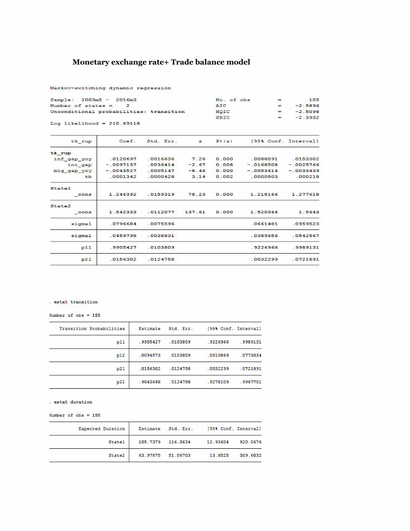
By applying 2-state Markov switching framework to monetary exchange rate model, we find
evidence of nonlinear relationship between monetary fundamentals and exchange rate as
demonstrated by the highly persistent appreciation and depreciation regimes. In particular, the
monetary fundamentals explain the behavior of Taka/Rupee exchange rate well as the
interpretation of coefficients render statistical significance for inflation differential, interest
differential, money growth differential and also for the non-monetary fundamental of trade
balance. In fact, the trade balance variable improves the fit of our model according to the regime
classification measure (RCM) values. The fundamentals used in the study are also in line with
the theory except for money growth differential, the coefficient of which shows a negative
relationship with exchange rate movement. Empirical evidence from the out-of-sample
forecasting exercise provides a mixed verdict. According to Diebold Mariano (DM) test statistic,
MS monetary model outperforms random walk for the one-month ahead forecast errors
1 The stylized facts on Bangladesh-India bilateral trade has been gathered from Rahman and Akhter (2016)
generated using a rolling window indicating predictive content of monetary fundamentals.. This
positive result, however, is not supported by the recursive window, the DM results for which are
statistically significant for the random walk model. On the other hand, static and dynamic
window mostly delivers insignificant MSE and MAE differences.
The study is organized as follows. In section 2, we discuss exchange rate modeling and
forecasting over the past 25 years with a focus on exchange rate series from a developing country
perspective. Section 3, 4 and 5 discusses the theory, data and methodology employed in this
study. In section 6, we estimate the Engel and Hamilton’s Markov switch model with monetary
fundamentals as exogenous variables and compare its forecast accuracy with the benchmark
model of random walk. Section 7 draws the conclusion.
2. Literature Review
2.1 Structural models of exchange rate determination
One of the earliest ways of exchange rate determination was the flow approach-the traditional
view that focused on demand and supply of trade flows in foreign exchange rate market.
However, with Bretton Woods summit’s decision to depart from fixed exchange rate system to
floating exchange rate, the flow approach soon lost its validity in the theoretical world and the
asset based models of the 1970’s such as PPP, UIRP, and monetary model became the more
predominant view to exchange rate determination. In addition, arrived different variants of the
monetary models such as the class of portfolio balance models2 of Hooper-Morton (1982) and
Frankel (1985), real differential model that each had monetary approach as a special case. These
structural models are based on the common, underlying assumption of rational expectation and
perfect capital mobility.
Modeling exchange rate with structural elements came under scrutiny with the advent of the
disconnect puzzle by Meese and Rogoff. Meese and Rogoff (1982) demonstrates how the
traditional asset based models fail to provide out of sample forecasts by root mean square
error(RMSE) criteria3 which lead the authors to conclude that there is considerable amount of
disconnect between exchange rate and macroeconomic fundamentals. The literature following
Meese and Rogoff is divided in opinion and progressed gradually through various attempts. As
Boughton (1988) specifically argues some of the empirical problems associated with the
monetary approach may be solvable by paying more attention to the specification of the
empirical relationships without calling into question the underlying monetary theory.
If it’s theory that must not be questioned, then much of the weight of the ongoing debate
surrounding structural model’s predictive ability shifts to methodological improvements. We
present some arguments of the debate in this section, not always in chronological order. For
example, Cheung, Chinn and Pascual (2005) tests the out-of-sample efficacy of some of the
2 These are the non-monetary class of asset-based models that assumes imperfect substitutability between domestic and foreign bonds by risk-averse agents 3 RMSE is a statistical criteria of measuring the difference between sample values and predicted values typically used to evaluate forecast accuracy
models of the nineties against benchmark model of random walk together with sticky price and
purchasing power parity using both error correction and first difference specification and finds
evidence of long-horizon predictability of exchange rate movement but not short-run. Similarly,
Mark (1995) uses Gaussian parametric and non-parametric estimate of the simple monetary
exchange rate model and finds random walk characterization at 1- and 4-quarter horizon but
long horizon predictability at 16 quarter. However, Killian (1999) modifies the bootstrap method
employed by Mark in a vector error correction framework and argues that because of presence
of nonlinearities in the data generating process, the bootstrap p-values of Mark’s long horizon
regression results are biased and thus mistakenly advocate long-horizon predictability of the
monetary model.
Mark and Sul (2001) implements panel specification in monetary model to mitigate previous
confounding results and examines if predictability of the model improves once cross-country
shocks are accounted for. The authors apply the specification on a panel of nineteen countries
with inferences being drawn from both asymptotic and bootstrap distribution and find that
exchange rates are co-integrated and with regard to forecastibility of the specification there
seems to be sufficient predictive power of monetary fundamentals in an out-of-sample
experiment generated from panel regression. Basher and Westerlund (2006) corroborate the
work of Mark and Sul (2001) and puts emphasis on the inference end of the test statistics
employed to panel data sets in the literature. By pooling parameters of both the forecasting
equation and the test statistics, the authors come to the conclusion of a larger power gain and
hence better exchange rate predictability of the monetary model than previous studies.
Besides monetary model and panel specification, other structural models that have seen modest
success at improving exchange rate forecast are external balance model by Gournichas and Rey
(2007) and Taylor rule fundamentals of Molodtsova and Papell (2008). Gournichas and Rey
(2007) uses ratio of net exports to net foreign assets as a trade balance variable to forecast one-
period-ahead forecasts of both trade and FDI-weighted exchange rate. The results of the study
render statistically significant test inferences of bootstrapped CW, DMW and ENC-NEW test
which are also robust to varying forecast window as reported in Rogoff and Stavrakeva (2008).
Molodtsova and Papell (2008) tests out-of-sample predictability of OECD countries currencies
(USD as the numeraire) in a Taylor rule specification with inflation gap, output gap and interest
rate as right hand side variables. The study provides evidence in favor of Taylor rule model that
yields higher forecast accuracy than random walk specification when inferences are made with
Clark-West procedure.
2.2 Non-linear modeling of exchange rate and fundamentals
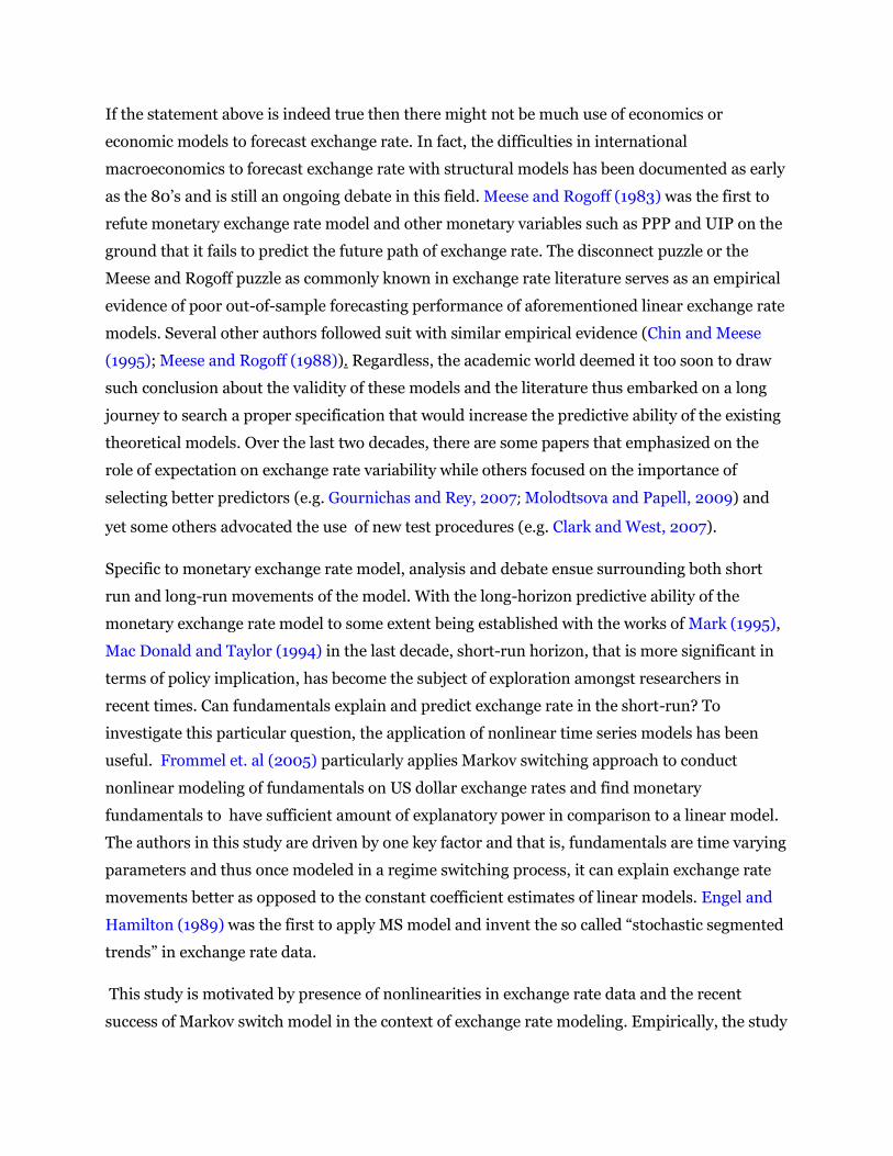
Figure1. Nonlinearities in exchange rate data
Figure 1. Stochastic segmented trends in dollar/mark, dollar/pound and dollar/franc exchange rates. Adapted from
"Long swings in the dollar: are they in the data and do markets know it" by C. Engel and J. D. Hamilton, 1990,
American Economic Review, 80, p. 690. Copyright 1990 by the American Economic Review.
Since late 80’s and early 90’s yet another body of academic literature emerged that aimed on
exploiting non-linearities4 in exchange rate process through Markov switching models- a
branch of statistical model that could capture “swings” or “segmented trends”, a typical
characteristic demonstrated by exchange rates after regime shift to floating exchange rate
system. It must be taken into account that the presence of non linearity in exchange rate data
was first detected by Hseih (1989)5. In the purview of non-linear models and its application on
exchange rate data, the aforementioned concept of long swings was first formalized by Engel
4 Non linearity in time series is a feature. It should be noted that there are distinct types of nonlinearity. According to Kaufmann et al. (2014), Markov switching dynamics are better for capturing “sudden” but “persistent” shocks as in developing countries and models such as ESTAR for large deviation from PPP as noticed in developed countries 5 Hseih (1989) employed Brock, Dechert and Scheinkman (BDS) test to establish nonlinear dependence in daily foreign exchange rates and thereby made comparison between types of nonlinearity.
and Hamilton (1990) with the particular application of Markov switch model on US dollar
exchange rate as depicted in Figure 1 above.
Amongst subsequent studies employing Markov Switch model, there exists some empirical
evidence in favor of nonlinear relationship between exchange rate and fundamentals albeit the
body of work to some extent is limited. In this regard, Cushman (2000) is an exception.
Beckmann and Czudaj (2014) methodologically improves Cushman’s results and considers a
multivariate framework for monetary exchange rate model for Canada/US exchange rate within
a MS-VECM6 framework to analyze how exchange rate adjusts to fundamental deviations and
the authors find empirical evidence of long-run relationship between exchange rate and
fundamentals. Frömmel, MacDonald, and Menkhoff (2005) studies Markov switching regime in
a monetary exchange rate model to explore which factors drive regime switches using Frankel’s
1979 variant of the model(MS-RID). The result shows evidence of nonlinear relationship
between monetary fundamentals and USD exchange rate of three currencies: Mark, Yen and
Pound Sterling. The time-varying coefficients of MS-RID are statistically significant while the
constant coefficients of RID model are not. More recently, Wu (2015) further corroborates the
modeling aspect of the studies cited above. While analyzing Asia Pacific country currencies he
incorporates time-varying transitional probabilities (TVTP)7 in the Markov switch model and
finds higher log-likelihood8 values for the model compared to a MS-RID. There is also evidence
of statistically significant variables in one of the regimes reconfirming economic fundamentals
are time varying. Grauwe and Vanteenkiste (2001) draws a distinction of the relationship
between exchange rate and fundamentals such as money supply, inflation and interest rate by
using monthly and quarterly data of both high and low inflation countries in a Markov switch-
autoregressive(MS-AR) framework. The results generate a certain pattern- high inflation
countries are marked by less frequent regime change while low inflation countries demonstrate
frequent structure break which lead the author to come to the conclusion that structural model
might work better for high inflation countries than low inflation countries.
Exchange rate forecasting has also sparked diverse results and opinions in the literature. The
predictability depends on multiple factors such as selection of key predictors(e.g. better
predictors for “appreciating” and “depreciating” regime), forecast horizon-one step or multi-
6 A vector error correction model augmented with Markov switching in mean and variance 7 An extension of the Markov switching model which allows the transition probabilities to vary subject to certain lagged observation 8Log-likelihood , a model selection criteria, that basically stands for log of the likelihood, that is, parameter estimates of a model that increase the occurrence of the data. Closer the log-likelihood value is to 1, better the fit of the model.
step, sample period, data frequency, forecast evaluation method and the methodology employed
(Rossi, 2013). Now, how effective is Markov switch, within a structural model framework, in
forecasting exchange rate? The answer is somewhat ambiguous. The literature is filled with
mixed evidence with some studies delivering positive forecasting performance while others
nodding in disagreement. Engel (1990)’s univariate process of exchange rate regime has been
well received in the exchange rate forecasting literature being the first of its kind in this field to
establish the nonlinear relationship between dollar/mark, dollar/exchange rate and its past
observation. However, it must also be noted that the study does not probe into the source of the
switch and it also received criticism in subsequent literature on its capacity to forecast. For
example, Engel (1994) ( wrong prediction- it shows depreciation of USD during early 80s when
it actually appreciated). Kaminsky (1993) emphasizes on the role of expectation and argues that
investors in the foreign exchange market are informed, so, other than taking into account past
observations of spot rate in the regime switching process as in Engel(1990), one must also focus
into announcements made by monetary policy authorities to better predict exchange rate path.
Markov switch/regime-switching process needs to incorporate such variables to predict better
and accurately. Kirikos (2011) compares forecasting ability of linear and nonlinear model and
finds random walk specification at short-horizon and linear structural model at long-horizon to
be more apt candidate of forecasting exchange rate. Dacoo and Satchell(1999) applies the basic
segmented trends model on DM/dollar exchange rate and analyzes as to why regime switching
model have not been able to provide satisfactory results in the previous literature. The authors
present an analytical discussion and argue that regime switching models can very easily have
higher MSE than RW model due to even slight regime misclassification error.
On a different note, Chen and Lee (2006) justify the use of Markov switch model to predict
exchange rate. By deriving a rational expectation model of exchange rate determination, the
authors show that exchange rate process is a state-dependent phenomenon, the states being
central bank’s intervention and central bank’s non-intervention.. In light of more recent
literature, Nikolsko and Prodan (2014) extends the study of Engel(1994) over a larger data set of
currencies of 12 OECD countries versus the dollar and reanalyzes forecastability of MS-RW
model using alternative test statistics/new test procedure and finds evidence of both short-
horizon and long-horizon predictability of the pure statistical model.
With regard to Markov switch testing the forecasting performance of monetary model, the study
of Frommel et. al (2005) is relevant again. The authors compare the forecasting ability of three
models using RMSE and MAE statistical measures, the three specifications being pure Markov
switch model, Markov switch model with fundamentals and the benchmark of random walk and
finds Markov switch with fundamentals with the best forecasting performance. At the same
time, the authors forecast over multi-periods of 1, 3 and 6 months and find over short-run,
random walk is the better model than Markov switch with fundamentals.
2.3 Developing and emerging country’s exchange rate series modeling and
forecasting: application of Markov Switch
In the previous subsections, we mostly discuss how exchange rate series have been modeled and
forecasted with respect to developed country currencies. In this section, we take upon the issue
keeping a focus on developing country currency analysis that has used the Markov switching
framework. For example, Chen (2006) use currencies from six developing countries such as
Indonesia, South Korea, Philippines, Thailand, Mexico and Turkey to establish the relationship
between interest rate and exchange rate volatility by segmenting the data into high volatility and
low volatility regime. The author finds that on increasing the interest rate, exchange rate
volatility exhibits a tendency to shift to high volatility regime and thus the authors conclude that
higher interest rate is not enough to safeguard exchange rate of these countries from a “crisis”
phase. Sinha and Kohli(2013) in their study tries to establish relationship between India’s
foreign exchange rate market and stock market on one hand and on the other tries to look at
how certain macroeconomic variables such as inflation differential, interest rate, current
account deficit. . Bakin, Anwer and Khan (2013) carries out a forecasting exercise on daily
Bangladeshi exchange rate series using various nonlinear models such as adaptive neuro fuzzy
inference system (ANFIS), MS-AR and and GARCH model. The study compares forecasting
performance of the aforementioned models through popular statistical measures such as MAPE
and RMSE and concludes that ANFIS model possesses the highest forecast accuracy out of all
three models. Shen and Chen (2006) apply Markov switching model on Taiwanese exchange
rate and draw a distinction between the segmented trends of developed and developing country
currencies- while developed economies have greater tendency to adhere to appreciation and
depreciation regime, developing countries demonstrate persistence in the appreciation regime.
3. The theory
In this section, we begin by discussing two parity or no-arbitrage conditions of exchange rate
determination in the goods and capital market, namely interest rate parity (IRP) and purchasing
power parity (PPP). Next, a theoretical dissection of the monetary exchange rate model is
undertaken-flexible, sticky price models are discussed with a focus on both the theoretical
interpretation and empirical advancement over time.
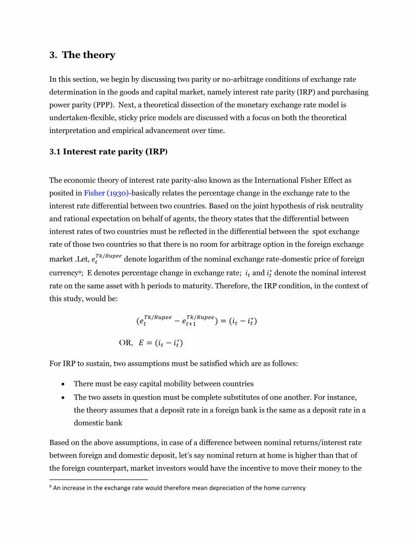
3.1 Interest rate parity (IRP)
The economic theory of interest rate parity-also known as the International Fisher Effect as
posited in Fisher (1930)-basically relates the percentage change in the exchange rate to the
interest rate differential between two countries. Based on the joint hypothesis of risk neutrality
and rational expectation on behalf of agents, the theory states that the differential between
interest rates of two countries must be reflected in the differential between the spot exchange
rate of those two countries so that there is no room for arbitrage option in the foreign exchange
market .Let, 𝑒𝑡𝑇𝑘/𝑅𝑢𝑝𝑒𝑒
denote logarithm of the nominal exchange rate-domestic price of foreign
currency9; E denotes percentage change in exchange rate; 𝑖𝑡 and 𝑖𝑡∗ denote the nominal interest
rate on the same asset with h periods to maturity. Therefore, the IRP condition, in the context of
this study, would be:
(𝑒𝑡𝑇𝑘/𝑅𝑢𝑝𝑒𝑒
− 𝑒𝑡+1𝑇𝑘/𝑅𝑢𝑝𝑒𝑒
) = (𝑖𝑡 − 𝑖𝑡∗)
OR, 𝐸 = (𝑖𝑡 − 𝑖𝑡∗)
For IRP to sustain, two assumptions must be satisfied which are as follows:
• There must be easy capital mobility between countries
• The two assets in question must be complete substitutes of one another. For instance,
the theory assumes that a deposit rate in a foreign bank is the same as a deposit rate in a
domestic bank
Based on the above assumptions, in case of a difference between nominal returns/interest rate
between foreign and domestic deposit, let’s say nominal return at home is higher than that of
the foreign counterpart, market investors would have the incentive to move their money to the
9 An increase in the exchange rate would therefore mean depreciation of the home currency
bank that pays higher nominal return. IRP, therefore, only exists when the expected nominal
rates are the same for domestic and foreign assets and hence, this parity condition is also
otherwise known as no-arbitrage condition. In the event there is any difference between the
nominal interest rates, the theory expects that an adjustment must occur through expected
appreciation or depreciation in the foreign or domestic currency. For instance, if domestic
interest rate is 5% and foreign interest rate is 3%, and then according to the theory, the investors
expect foreign currency to appreciate by 2% or by the same count, investors expect the domestic
currency to depreciate by 2%. Now to justify as to why domestic currency depreciate of the
country with the higher interest rate, let us consider the aggregate money demand model.
Money demand comes in to the picture as interest rate influences both individual and aggregate
money demand. According to aggregate money demand model, a higher interest rate, which
basically means the opportunity cost of holding money is higher, causes demand for money to
decrease which eventually makes the currency to depreciate.
Now, this equity between interest rate in different countries in the real world does not always
exist because of failure of the assumptions to hold or otherwise and thus allow traders to avail
arbitrage option position. Chinn and Meredith (2004) suggests that interest rate differentials
are “biased predictors” of exchange rate movements in the short run, thus, resulting in signs
opposite to what theory dictates over a short horizon of 12 months. The authors also note that
the theoretical linkage between interest rate differential and exchange rate movement is more
apparent over horizons of 5 years or 10 years.
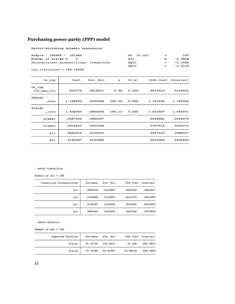
3.2 Purchasing power parity (PPP)
The parity theory of exchange rate, based on law of one price, allows one to estimate what the
exchange rate between two currencies would have to be in order for the exchange to be on par
with the purchasing power of the two countries' currencies over the same basket of good. There
are two different versions to the theory-popularized by Gustav Cassel-real exchange rate is
considered to be 1 in the absolute version and in the relative version there is no expected
movement in real exchange rate and changes in the exchange rate is equal to changes in relative
national price levels. Let p* be logarithm of price level in India; p be logarithm of price level in
Bangladesh; 𝑒′𝑡𝑇𝑘/𝑅𝑢𝑝𝑒𝑒
denote real exchange rate10;
10 Real exchange rate is nominal rate adjusted for price level
Absolute version of PPP 𝑒′𝑡𝑇𝑘/𝑅𝑢𝑝𝑒𝑒
= 𝑒𝑡𝑇𝑘/𝑅𝑢𝑝𝑒𝑒
(𝑝 − 𝑝 ∗)
Therefore, 𝑒𝑡𝑇𝑘/𝑅𝑢𝑝𝑒𝑒
= 𝑝 − 𝑝 ∗
Relative version of PPP ∆𝑒𝑡𝑇𝑘/𝑅𝑢𝑝𝑒𝑒
= ∆(𝑝 − 𝑝 ∗)
Or, ∆𝑒𝑡𝑇𝑘/𝑅𝑢𝑝𝑒𝑒
= (𝜋 − 𝜋 ∗)
To elaborate further, Cassel (1918) points out in simple terms that whatever a basket of goods
and service cost in one country, once converted to another currency, one should be able to
purchase same level of goods and services given a floating exchange rate system is prevalent in
both countries. For example, suppose there is increase in inflation in the domestic country due
to monetary disturbance and the domestic basket of good rise in price. If the nominal exchange
rate remains the same then this means that foreign residents can no longer buy the same level of
goods and services as their currency is undervalued with comparison to domestic currency and
the domestic currency on the same count is overvalued. In such a situation, according to PPP
theory, the nominal exchange rate must go through an adjustment process. With the domestic
currency being overvalued, it makes foreign goods cheaper which induces domestic residents to
buy goods from abroad. This increases the supply of domestic currency and at the same time
puts an upward pressure on demand for foreign currency which eventually causes foreign
currency to appreciate and domestic currency to depreciate as a mechanism to settle down to
PPP exchange rate.
One practical implication of PPP is the Big Mac index (Economist, 1986) which is basically used
to see if nominal exchange rate of a country is undervalued or overvalued compared to the price
of a Big Mac, a popular hamburger served at fast food chain MacDonald’s. Let’s say if the price
of a Big Mac in US is $4.7 while in China it is about 2.7 yen then we can say that yen is
undervalued and there is pressure on yen to appreciate in value to rise up to the PPP exchange
rate.
Data, however, rejects this hypothesis which leads us to the PPP puzzle postulated in Rogoff
(1996). On theoretical disposition, the fact that PPP deviates in the short run is inevitable given
the nature of international transaction that includes trade barriers such as tariffs and also
transaction cost. To put it in other words, there is a short-run deviation from PPP owing to
these factors. Therefore the PPP debate or the validity of the PPP hypothesis hinges more
around its long-run validity in the literature and thus the use of real exchange rate have been
more useful to economists. Nonlinear modeling of real exchange rate with smooth version of
threshold autoregressive11 resolves the PPP puzzle as can be seen in the work of Taylor, Peel and
Sarno(2001) who find real exchange rate data to be nonlinearly mean reverting and the half-life
to be much less, particularly under 3 years, thus, favoring PPP evidence in the long-run.
In the forecasting literature, the general consensus is that PPP forecasts well for long-horizon
not short horizon (Ching, Chinn and Pascual, 2005; Engel, Mark and West, 2007). However,
one strand of recent forecasting literature also gives positive implication for accounting for
smooth nonlinearities in nominal exchange rate data that result in PPP as a better exchange rate
predictor. For example, Suarez and Lopez (2010) employs smooth transition error correction
model (STEC)12 on panel data of nominal exchange rate and CPI levels and finds the model to
beat random walk specification at both short and long horizon and over different forecast
windows, implying robustness of the out-of-sample results. model for nominal exchange rate
forecasting. On a slightly different note, Bjornland and Hungnes (2006) stresses that
importance of interest rates in forecasting exchange is substantial- a structural model
combining both PPP fundamentals and interest rate differential beat random walk rate-out-of-
sample.
3.3 Monetary theory of exchange rate determination
The monetary approach to exchange rate determination, as the name suggests, puts emphasis
on the money market-through demand for and supply of money-as a way of determining
exchange rate. Central to a monetary model is the money demand function and three crucial
assumptions following the flexible version of the monetary approach (also known as Frenkel and
Bilson (1978) ) which are as follows:
11 According to Taylor and Taylor(2004), STAR models address the goods aggregation problem-as transaction costs are different for different goods, more and more thresholds will be breached and the speed of adjustment, as a result will also vary across goods 12 On the other hand, STEC model
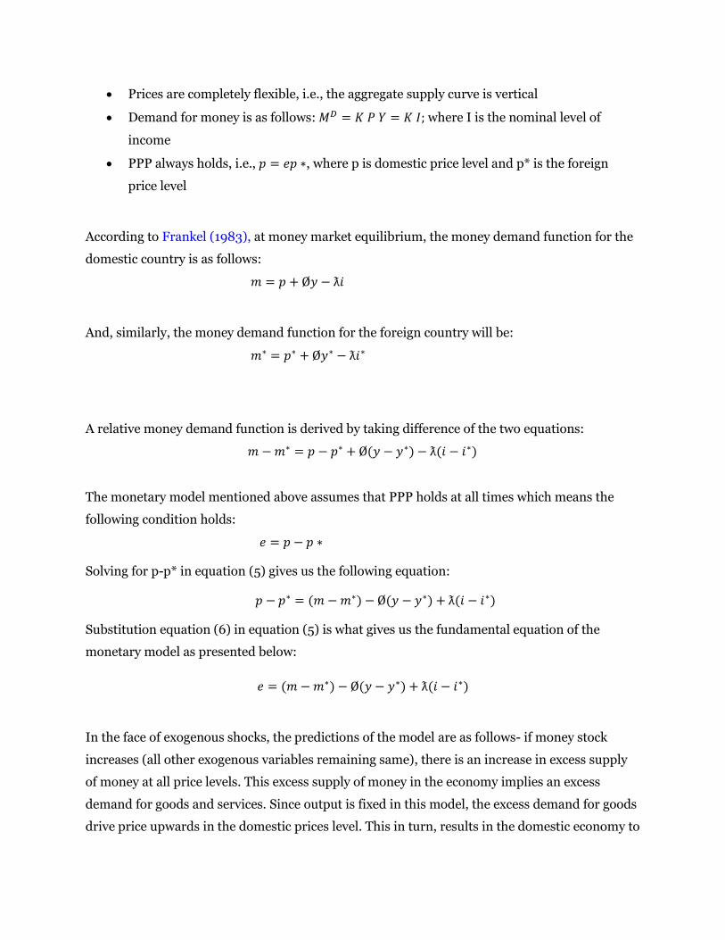
• Prices are completely flexible, i.e., the aggregate supply curve is vertical
• Demand for money is as follows: 𝑀𝐷 = 𝐾 𝑃 𝑌 = 𝐾 𝐼; where I is the nominal level of
income
• PPP always holds, i.e., 𝑝 = 𝑒𝑝 ∗, where p is domestic price level and p* is the foreign
price level
According to Frankel (1983), at money market equilibrium, the money demand function for the
domestic country is as follows:
𝑚 = 𝑝 + Ø𝑦 − ƛ𝑖
And, similarly, the money demand function for the foreign country will be:
𝑚∗ = 𝑝∗ + Ø𝑦∗ − ƛ𝑖∗
A relative money demand function is derived by taking difference of the two equations:
𝑚 − 𝑚∗ = 𝑝 − 𝑝∗ + Ø(𝑦 − 𝑦∗) − ƛ(𝑖 − 𝑖∗)
The monetary model mentioned above assumes that PPP holds at all times which means the
following condition holds:
𝑒 = 𝑝 − 𝑝 ∗
Solving for p-p* in equation (5) gives us the following equation:
𝑝 − 𝑝∗ = (𝑚 − 𝑚∗) − Ø(𝑦 − 𝑦∗) + ƛ(𝑖 − 𝑖∗)
Substitution equation (6) in equation (5) is what gives us the fundamental equation of the
monetary model as presented below:
𝑒 = (𝑚 − 𝑚∗) − Ø(𝑦 − 𝑦∗) + ƛ(𝑖 − 𝑖∗)
In the face of exogenous shocks, the predictions of the model are as follows- if money stock
increases (all other exogenous variables remaining same), there is an increase in excess supply
of money at all price levels. This excess supply of money in the economy implies an excess
demand for goods and services. Since output is fixed in this model, the excess demand for goods
drive price upwards in the domestic prices level. This in turn, results in the domestic economy to
become under competitive. So for PPP to hold, domestic currency must depreciate in terms of
the foreign currency.
Let us now consider the exogenous shock of an increase in the level of income. At 𝑝0, there is an
excess demand for money which implies an excess supply of goods and services. This leads to a
fall in the domestic price level and therefore the domestic economy becomes more competitive
and hence an appreciation of the currency is required so that PPP holds. From this we can
deduce that, in a monetary model, an increase in real income leads to an appreciation of the
domestic currency.
Lastly, an increase in price level will see an increase in the slope of the PPP curve. At the original
nominal exchange rate, the domestic economy becomes over competitive; hence the domestic
currency must appreciate. To summarize, according to monetary model prediction, a rise in the
foreign price level leads to an appreciation of the domestic currency and vice versa.
Simultaneously, if we relax the assumption of PPP but let UIP hold, which seemed to be the
scenario post floating regime leading to volatile nature in the exchange rate, we have the sticky
price version of the monetary model( aggregate supply curve is vertical) developed by
Dornbusch. This version assumes instead that prices are sticky in the short run and hence an
initial increase in interest rate (let’s say due to reduction of money supply in the economy)
would cause capital inflow that would result in appreciation13 of the nominal exchange rate. In
other words, the model predicts a negative coefficient for interest rate differential in the short-
run and a positive coefficient in the long-run where PPP hold.
Based on the monetary theory of exchange rate determination, the study applies the following
sticky-price variant of the monetary exchange rate model specification with a trade balance
variable augmented in it:
𝑒𝑡 = (𝑚 − 𝑚 ∗) + (𝑖 − 𝑖 ∗) + (𝜋 − 𝜋 ∗) + (𝑇𝐵)14
Where, 𝒆𝒕 is the log of Taka/Rupee exchange rate; asterisks denote variables for India;
(𝒎 − 𝒎 ∗)is the money supply differential; (𝒊 − 𝒊 ∗) is the interest rate differential and(𝝅 − 𝝅 ∗)
is the inflation differential between the two countries. A trade balance variable, 𝑻𝑩 is augmented
13 This appreciation of the exchange rate is termed as “overshooting” in the literature , an appreciation that is beyond the PPP level 14 The study does not consider any specific variant of the monetary models of exchange rate determination because of lack of monthly data on income for Bangladesh. However, the model can be considered close to the sticky price version of the monetary model as it uses inflation differential as one of the regressors
in the standard monetary exchange rate model to see if there’s any impact of the existing and
much debated trade imbalance between India and Bangladesh on the bilateral exchange rate of
Taka/Rupee. It should be noted that Hooper and Morton (1982) was the first to incorporate a
trade balance variable in the monetary exchange rate model but the authors did so with an
intention to use it as a broad substitute for stock of balances, what came to be known as the
portfolio balance determination of exchange rate in the literature. The study here uses trade
balance only as the difference between import and export between the two countries, not as a
relative change in trade balance, i.e., TB-TB* as used in Hooper and Morton (1982).
4. Data
In order to conduct the estimation, the study uses monthly data from May 2003 to March 2016
for India and Bangladesh International Financial Statistics (IFS) databsase. The time period is
chosen from May 2003 onwards to reflect the shift to floating exchange rate regime by
Bangladesh Bank on the same year. All the estimation is performed in statistical software
STATA.
The dependent variable, nominal exchange rate is quoted as units of domestic currency per
foreign currency, i.e., Bangladesh taka per Indian Rupee, and is made to undergo log
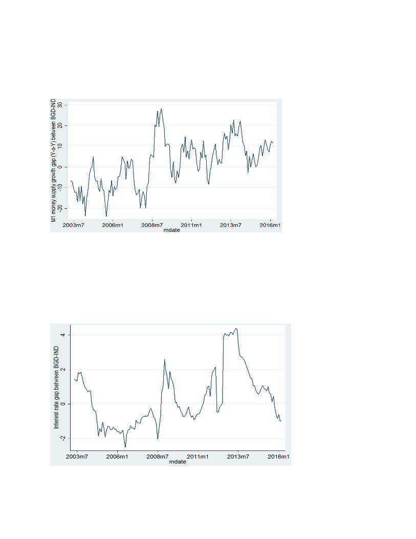
transformation and labeled as “ltk_rup”. Relative changes in monetary fundamentals such as
Indian money supply and Bangladeshi money supply, m1 and m2 (in million USD), are labeled
as “m1g_gap_yoy” and “m2g_gap_yoy” respectively and calculated as the percentage change
during the last twelve months in the domestic country against the percentage change in the last
twelve months in the foreign country and can be represented as follows:
∆𝑚𝑡 =𝑚𝑡
𝑑𝑜𝑚𝑒𝑠𝑡𝑖𝑐−𝑚𝑡−12𝑑𝑜𝑚𝑒𝑠𝑡𝑖𝑐
𝑚𝑡−12𝑑𝑜𝑚𝑒𝑠𝑡𝑖𝑐 −
𝑚𝑡𝑓𝑜𝑟𝑒𝑖𝑔𝑛
−𝑚𝑡−12𝑓𝑜𝑟𝑒𝑖𝑔𝑛
𝑚𝑡−12𝑓𝑜𝑟𝑒𝑖𝑔𝑛
15
The relative change in CPI inflation, labeled as “inf_gap_yoy” (in %) is also calculated in the
similar way as shown in the equation above. The variables are calculated this way to avoid any
seasonal effects at an annual lag in the data and thus ensure variance stability necessary to
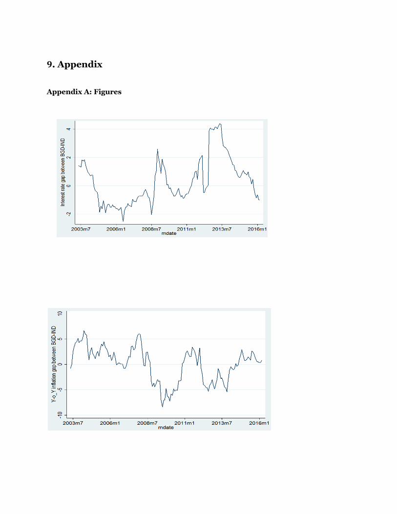
conduct the analysis. The interest rate gap, labeled as “int_gap”, is a growth variable in itself and
is simply calculated by taking the difference between Bangladesh Bank’s deposit rate and India’s
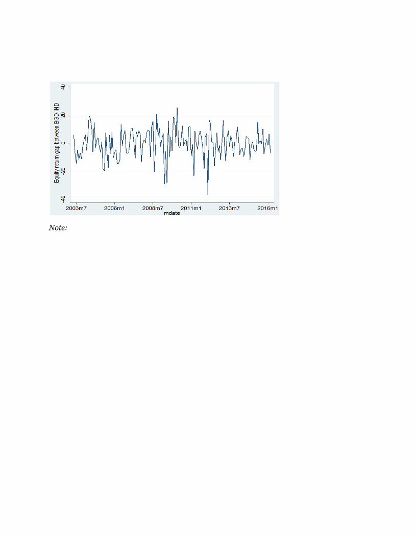
10-year government securities rate. An alternative to this variable is considered by taking the
difference between Bangladesh stock exchange (BSE) equity return and Indian Stock Exchange(
BSE) equity return, labeled as “eqret_gap”(in %).Finally, the trade balance variable augmented
in the framework is calculated as the difference between Bangladesh import to India (in million
USD) and Indian export to Bangladesh (in million USD) as recorded in Bangladesh’s current
account.
15 The month-on-month change of the same variables are calculated using a lag of one month: ∆𝑚𝑡 =
𝑚𝑡𝑑𝑜𝑚𝑒𝑠𝑡𝑖𝑐−𝑚𝑡−1
𝑑𝑜𝑚𝑒𝑠𝑡𝑖𝑐
𝑚𝑡−1𝑑𝑜𝑚𝑒𝑠𝑡𝑖𝑐 −
𝑚𝑡𝑓𝑜𝑟𝑒𝑖𝑔𝑛
−𝑚𝑡−1𝑓𝑜𝑟𝑒𝑖𝑔𝑛
𝑚𝑡−1𝑓𝑜𝑟𝑒𝑖𝑔𝑛
5. Methodology
5.1 Basic statistical issues in nonlinear time series analysis
We begin this section by establishing some of the salient features of non-linear time series and
into matters pertaining to detection of it and selection of appropriate test statistics. Next, we
move onto the second part of our methodology which entails a discussion of the Markov switch
model employed for our parameters. The third sub-section carries out a discussion of various
forecasting schemes, test procedures employed in this study to decide the better competing
model.
5.1.1 The notion of unit root
The term unit root is synonymous to non-stationary, a property that embodies a general
tendency of variables to increase over time. Statistically speaking, this would mean that the
mean, variance and covariance of the series are all time-dependent. In presence of unit root,
spurious regression, a term coined by Granger and Newbold (1974) becomes prevalent, i.e.,
there might not be any meaningful relationship between the regressor and the regressant but
estimates might still be highly statistically significant or vice versa. A simple example of non-
stationary time series is a random walk as in the following equation:
𝑦𝑡 = 𝜌𝑦𝑡−1 + 휀𝑡16
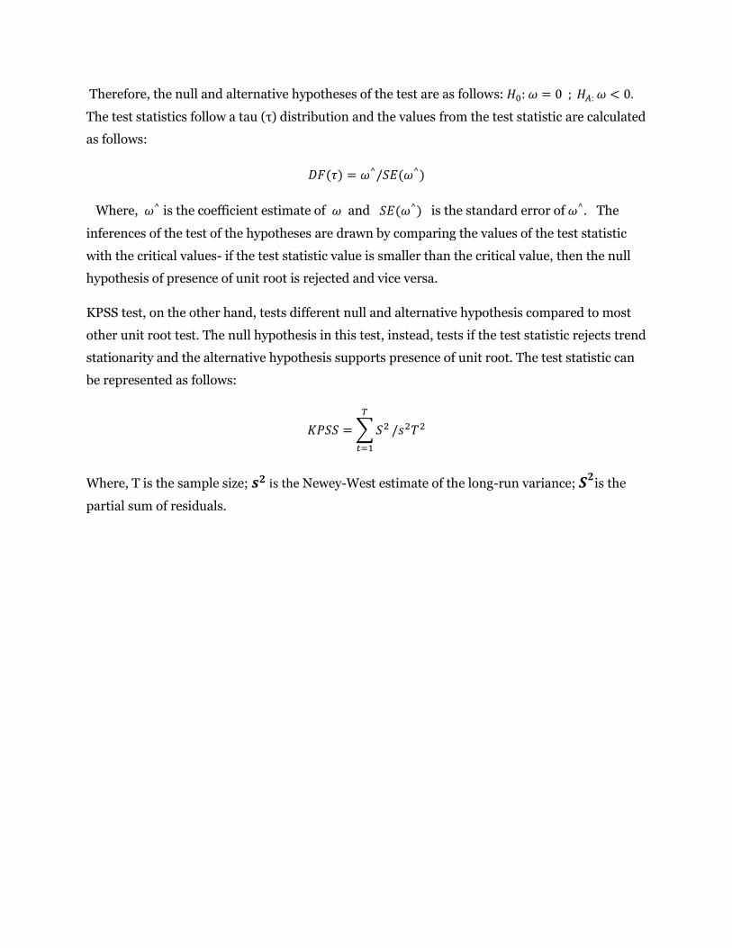
Unit root tests, therefore, test the following null hypothesis of ρ equal to 1 to alternative
hypothesis of ρ<1.Unit root in data is cured by taking first differences17 of the time series in case
of random walk without drift or pure random walk. The following equation for series 𝑦𝑡
illustrates difference stationary process:
∆𝑦𝑡= 𝑦𝑡 − 𝑦𝑡−1= 휀𝑡
16 Here et is a white noise error term with zero mean and constant variance, I.e. stationary
17 There can be instances where time series data requires second differencing or third differencing depending on the number of unit root present in the data, hence, a series is said to integrated to the order of 1,i.e., I(1) if it has been differenced once or integrated to the order of n, I(n), if differenced n times.
Certain types of time-series data might also be a trend stationary18 process. This is true for data
in which the mean is not constant but variance is and hence requires the deterministic trend to
be removed by the process of de-trending, i.e., subtraction of the mean of 𝑦𝑡 from 𝑦𝑡 . The
following equation represents a trend stationary process:
∆𝑦𝑡= 𝛽1 + 𝛽2𝑡= 휀𝑡
5.1.2 The notion of nonlinearity
To understand the idea of nonlinear process in time series, let us first consider what linear
adjustment could mean. Simply put a linear equation has variables raised to the power of one
and demonstrates constant coefficients. For example, consider a situation where investment is a
constant proportion of investment as in the following equation:
𝑖𝑡 = 𝛽(𝑐𝑡 − 𝑐𝑡−1)+𝑒𝑡
On other hand, non linear variables are variables that grow exponentially. Most time series
data exhibit nonlinear dynamics in its data generating process and perhaps they do so in a more
complex manner than the aforementioned examples of nonlinearity. Variables such as exchange
rate, stock prices have undergone structural changes and as a result have prompted researchers
to abandon typical linear difference equation models and drift towards the use of nonlinear
models to explain nonlinear behavior in time series. For example, Hamilton (1989) first used
nonlinear model to demonstrate the cyclical behavior of booms and bust in U.S. output growth.
Regime switching model is one class of nonlinear models where the particular value of the
dependent variable depends on the state of the system which is a state of dynamic equilibrium19.
To illustrate better, consider the role of certain economic variables such as unemployment rate-
during recession, unemployment rate is more likely to show upward adjustment than
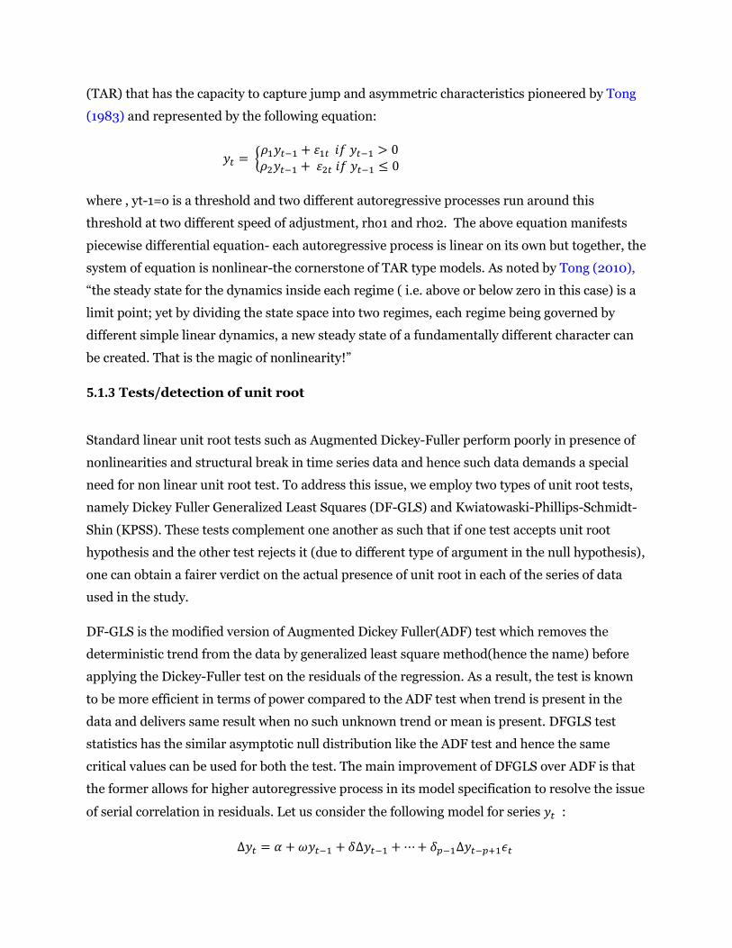
downward. The simplest example of a regime switching model is a threshold autoregressive
18 The distinction between a unit root process and a trend stationary process is that the former has non-mean reverting properties while the latter possess mean-reverting properties. Both are non-stationary processes. 19
(TAR) that has the capacity to capture jump and asymmetric characteristics pioneered by Tong
The model draws interesting and useful inferences about the transition probabilities and other
model parameters. For example, if probability of being a certain state is high or close to 1 then
that shows persistence on behalf of the data. The coefficient of mean, on the other hand, gives an
estimate of the trend of the data- a positive and a statistically significant mean represents
uptrend in the data or depreciation of exchange rate and a negative and a significant means a
downtrend in the data or appreciation of the exchange rate. The sigma gives inference about the
volatility shifts in the data.
To analyze the role of monetary fundamentals on exchange rate dynamics, we also include
fundamentals in our Markov switching model in mean and variance which can be represented as
follows:
𝑒𝑡 = µ𝑠𝑡+ 𝛽 Xt +𝜎𝑠𝑡
휀𝑡 휀𝑡∿𝑁(𝑜,1)
Where, 𝛽 is kept constant across the two states and represents a vector of exogenous variables
such as money differential, interest and inflation differential and trade balance.
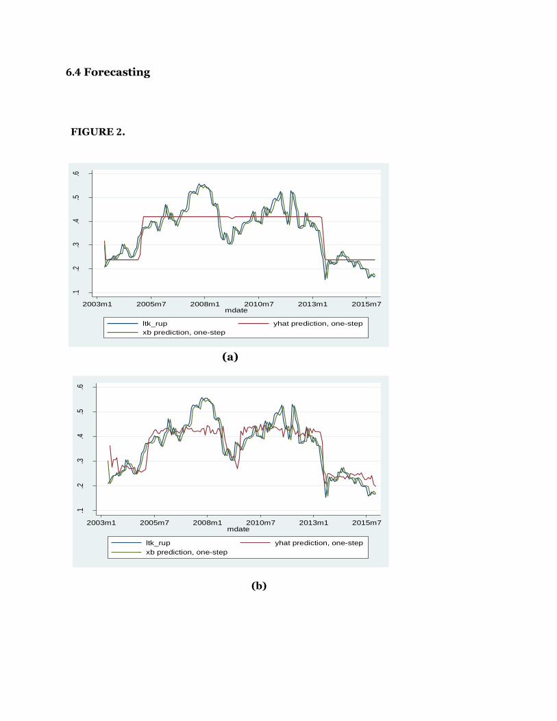
5.3 Forecasting
5.3.1 Key methodological factors in forecasting exchange rates
Other than selection of model and macroeconomic predictors, what’s equally important for a
successful exchange rate forecast is the choice of forecasting schemes, forecast horizon and the
evaluation methods to judge the forecast results. It’s this lack of robustness to aforementioned
criterion that makes exchange rate forecasting a daunting task. The literature on this end is
abundant with contradicting results and exchange rate forecasting is seen to vary over different
time periods and also vary depending on whether they are in-sample or out-of-sample. Rossi
(2013) notes that certain predictors forecast well in-sample while others forecast better out-of-
sample. The author further stresses the importance of forecast horizon, h, and that a predictor’s
predictive ability of exchange rate also depends on it. In Chin, Cheung and Pascual’s 1995 paper
we see that monetary fundamentals fail at making prediction at short-horizon, i.e., one-month-
ahead prediction, while Mark (1995) at the same time show evidence for monetary
fundamentals’ long-horizon predictability at 3 to 4 year horizon. Rossi (2013) also adds that
exchange rate forecasting is neither robust to the forecast sample or the out-of-sample forecast
period that is used for forecast evaluation. In this regard, the author cites the work of
Giacommini and Rossi(2010) who find that the forecastability of UIP and Taylor rule
fundamentals change over different out-of-sample periods with respect to a random walk
benchmark in each case.
The importance of the choice of a benchmark model was also emphasized by the author who
notes that the random walk without drift is the consistent benchmark model for exchange rate
forecasting all throughout the literature. The most common forecast methodologies used in the
literature are rolling and recursive forecast schemes. The rolling window size varies across
papers but typically ranges from 50 to 120 for monetary fundamentals. For evaluating forecast,
the three typical loss functions that are used are mean square error (MSE), root mean square
error (RMSE) and also mean average error (MAE). Alternatively, another forecast evaluation
tool is the direction of change statistic, a statistic that calculates the sign of change in forecast of
exchange rate (e.g. Engel (1994)). To assess the significance of forecast performance, the author
makes distinction between out-of-sample” absolute” and “relative”20 tests of forecast accuracy,
20 The relative tests of forecast accuracy in exchange rate literature refer to Diebold and Mariano, Clark and West and ENC-NEW test procedures etc.
noting that the former is useful for measurement of optimal forecast and the latter for the
purpose of evaluating which forecast is best among the competing models with RW as the
benchmark model.
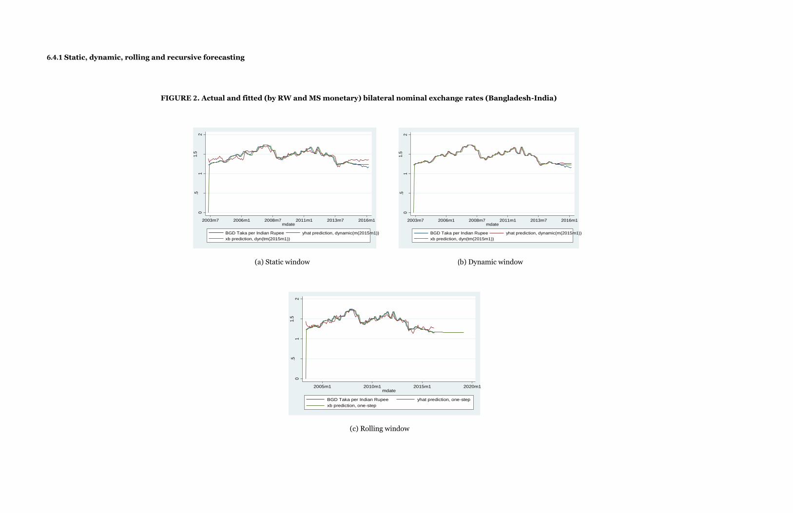
5.3.2 Forecasting schemes
Static vs. dynamic window
Static forecasting as the name suggests assumes that the world remains the same and makes use
of actual data to forecast out-of-estimation, one-step-ahead errors. This basically means that
once forecast errors are generated it can be compared with real world data , which is available to
the user, to judge the performance of the model. This type of forecasting is known as the ex-post
forecast. Assuming the world is static, the forecasting scheme does not include any lagged
dependent variable. Let us consider the concept in a linear regression framework:
𝑦𝑡 = 𝑋𝑡 𝛽𝑡 + 휀𝑡
Dynamic forecasting, on the other hand, is quite opposite to static forecasting in the sense that it
produces ex-ante forecast where actual values outside the estimation period are not available to
the modeler. Another way to distinguish it from static forecasting is the fact that it incorporates
a lagged dependent variable in its specification as follows:
𝑦𝑡 = 𝑋𝑡 𝛽𝑡 + 𝑦𝑡−1 + 휀𝑡
Rolling vs. recursive window
Rolling forecasting is conducted by using the most recent observation, say n, and thus
progressively moves forward over time, t. A simple representation of a rolling regression would
be as follows:
𝑦𝑡(𝑛) = 𝑋𝑡(𝑛) 𝛽𝑡(𝑛) + 휀𝑡(𝑛)
In a rolling window regression the most recent observations are used in a add-and- drop
manner. For example, if the in-sample portion21 is from 1998:01 to 2008:01 and the out-of-
sample portion is 2008:02 to 2016:01, then as a first step the model will estimate in-sample
using data from 1998:01 to 2008:01 to forecast 2008:02. Next, the forecasting model will drop
the first observation and add the recently projected value to re-estimate the model by using
observation from 1998:02 to 2008:02 to forecast 2008:03 and so on. It is because of this add
and drop process, rolling regression retains a fixed window of data each time to re-estimate the
model and predict future values.
Recursive approach instead uses an increasing window of data to predict future values and as
such makes use of all past observations. For example, given the same aforementioned in-sample
and out-of-sample periods, this approach will as a first step estimate the model in-sample by
using data from 1998:01 to 2008:01 to forecast 2008:02 and in the next step, it will re-estimate
model parameters from 1998:01 to 2008:02 to forecast 2008:03 and etc.
5.3.3 Forecast evaluation method
Through our comparison of forecast errors between the two competing models in, we address
one of our key research questions- do macroeconomic fundamentals, that are of great theoretical
interest to researchers, determine the future path of exchange rate or is the alternative of no
exchange rate predictability or a random walk model forecast is just as good or better. To this
end, we employ two loss functions and Diebold Mariano test statistics to derive the forecast
accuracy results.
Comparing statistical measure of forecast accuracy
Central to the idea of forecast accuracy measurement is a loss function, L (e). So basically, when
any forecast is produced one wishes to assess the expected loss associated with each of the
forecast- higher the loss, lower the accuracy and vice versa. Typically, forecast accuracy is
evaluated by using the one-step-ahead, out-of-sample forecast error22 and the sum of the
21 The first step to a successful forecasting is to divide the data into two segments- the “fitting segment” or the in-sample portion and the “forecasting segment” or the out-of-sample portion (Montgomery, Kulhaci and Jennings, 2008). 22 The distinction between residual and the forecast error is that the former is the difference between the observed and the fitted value ,i.e., it arises from the model-fitting process while the latter is the error made while forecasting the variable/variables of interest
squared forecast error23 is one such loss function that is widely used in the literature to gauge
statistical superiority of competitive models. It is represented as follows:
𝑀𝑆𝐸 = 𝜎𝑒(1)2 =
1
𝑛 ∑ [𝑒𝑡
𝑛𝑡=1 (1)]2
We also apply another loss function, namely MAE, to check robustness of our results across
different loss criteria. It can be represented as follows:
𝑀𝐴𝐸 =1
𝑛 ∑ [𝑒𝑡
𝑛𝑡=1 (1)]
Testing for equal predictive ability
To compare MSE’s across the two models, we simultaneously employ forecast evaluation
technique of testing for equal predictive ability between two forecasts by carrying out minimum
mean square forecast error test- also termed as the “MSE dominance” approach in the
literature- as a way of determining the predictive content of monetary fundamentals to exchange
rate. The head-to-head test of forecast accuracy measures of each of the model, based on a loss
differential function, is considered a better approach to forecast evaluation that uses MSE on a
stand-alone basis, according to empirical evidence.
In hypothesis testing terms, we are basically testing the following accuracy hypothesis (Diebold,
2007):
𝐸[𝐿(𝑒𝑡+ℎ,𝑡𝑀𝑆 )] = 𝐸[𝐿(𝑒𝑡+ℎ,𝑡
𝑅𝑊 )];
Against the alternative that the one or the other is better, i.e.,
𝐸[𝐿(𝑒𝑡+ℎ,𝑡𝑀𝑆 )] > 𝐸[𝐿(𝑒𝑡+ℎ,𝑡
𝑅𝑊 )] or, vice versa24
Equivalently, what the equal predictive ability hypotheses above tell us is that the expected loss
differential from the models is zero:
𝐸(𝑑𝑡) = 𝐸[𝐿(𝑒𝑡+ℎ,𝑡𝑀𝑆 ) − 𝐸[𝑙(𝑒𝑡+ℎ,𝑡
𝑅𝑊 )] = 0
23 By applying sum of the squared forecast error or MSE, one assumes a quadratic loss function of the form, 𝐿 = 𝑒2 24
The study uses Diebold and Mariano (1995) test statistic to compare predictive accuracy across
models. The DM test statistic is asymptotically normally distributed under the null hypothesis of
no difference in MSE or MAE. The inference from the test statistic is interpreted as follows: if
the DM test statistic falls outside the range of the critical values or are too extreme, the null
hypothesis of no difference will be rejected. That is, |DM|>𝑍𝛼/2, where 𝑍𝛼/2 is standard z-value
from standard normal table and 𝛼 refers to desired level of significance.
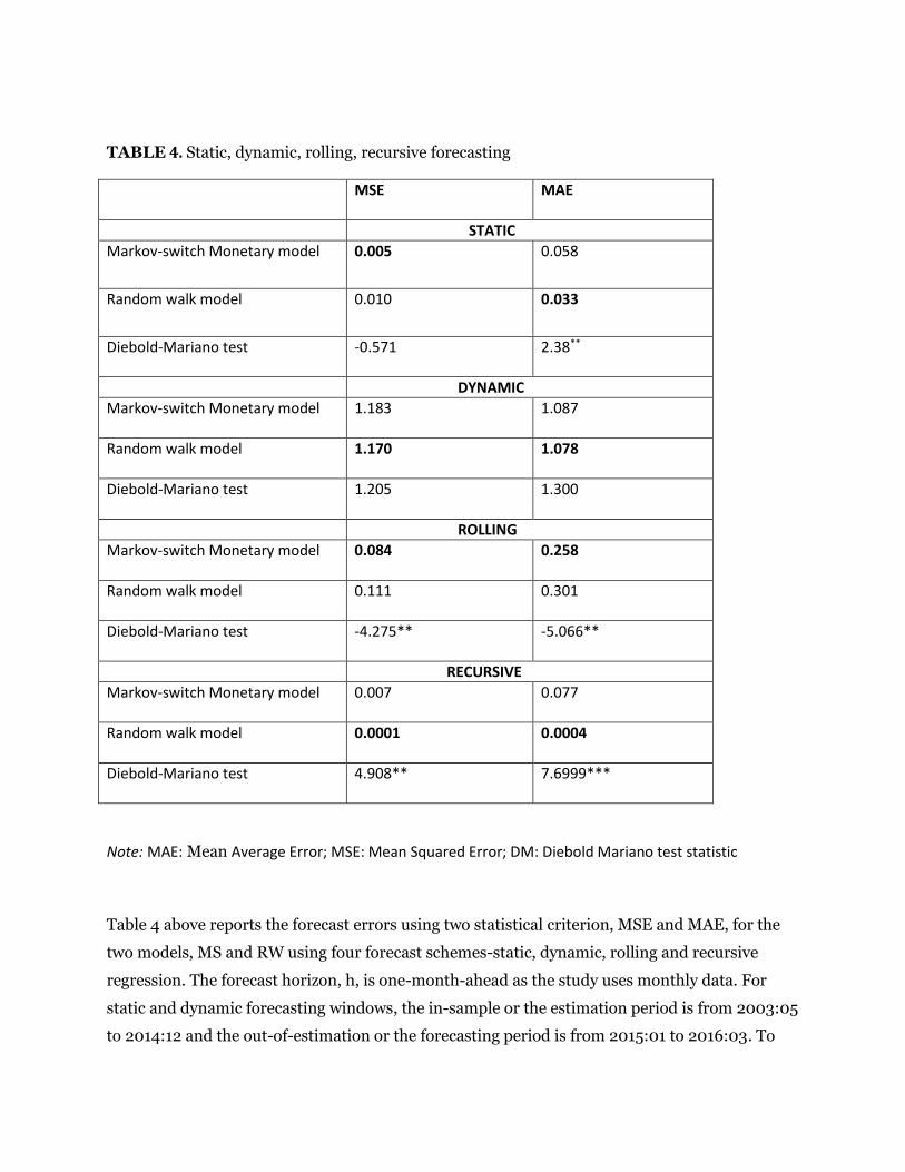
6. Results
6.1 Descriptive statistics
TABLE 1. Descriptive statistics
Mean Std. Dev CV Min Max
𝒆𝒕 1.44 0.15 0.11 1.15 1.74
𝝅𝒕 − 𝝅𝒕∗ 0.02 3.39 144.55 -8.43 6.68
𝒊𝒕 − 𝒊𝒕∗ 0.31 1.63 5.33 -2.51 4.39
𝒎𝟏𝒈𝒕 − 𝒎𝟏𝒈𝒕∗ 1.73 11.27 6.51 -23.83 28.39
𝒎𝟐𝒈𝒕 − 𝒎𝟐𝒈𝒕∗ 2.82 12.83 4.55 -21.87 34.13
𝒓𝒕 − 𝒓𝒕∗ -0.20 10.17 -51.35 -36.84 25.37
𝑻𝑩𝒕 (𝑼𝑺$) 263.12 141.64 0.54 103.17 657.92
Table 1 reports descriptive statistics for the following variables- 𝑒𝑡the monthly levels of
taka/rupee exchange rate and a set of fundamentals such as 𝜋𝑡 − 𝜋𝑡∗ , the percentage difference
between foreign and domestic CPI inflation; 𝑖𝑡 − 𝑖𝑡∗, the difference in domestic and foreign
interest rates; 𝑚1𝑔𝑡 − 𝑚1𝑔𝑡∗ , the percentage difference between domestic m1 money supply
growth and foreign m1 money growth; similarly, 𝑚2𝑔𝑡 − 𝑚2𝑔𝑡∗ , the difference between domestic
m2 money growth and foreign m2 money growth; 𝑟𝑡 − 𝑟𝑡∗ , the difference between domestic
stock exchange equity return and foreign stock exchange equity return; and the difference
between import and export trade figure with foreign country, 𝑇𝐵𝑡. The mean values for each of
the series are moderate but the mean value for 𝑇𝐵𝑡 is quite high. The standard deviation for 𝑒𝑡,
𝜋𝑡 − 𝜋𝑡∗, 𝑖𝑡 − 𝑖𝑡
∗ are somewhat close to unity and on the other hand, 𝑚1𝑔𝑡 − 𝑚1𝑔𝑡∗ , 𝑚2𝑔𝑡 −
𝑚2𝑔𝑡∗ , 𝑟𝑡 − 𝑟𝑡
∗, 𝑇𝐵𝑡 demonstrate very high standard deviation. The coefficient of variation (CV),
which is the ratio between standard deviation and the mean, indicate 𝜋𝑡 − 𝜋𝑡∗ and 𝑟𝑡 − 𝑟𝑡
∗ series
as highly volatile in terms of magnitude. The difference between min and max values, which is a
measure of variability, are different for each fundamental.
6.2 Stationarity test
TABLE 2. Unit root test
DF-GLS
KPSS
𝒆𝒕
-1.129
0.426**
𝝅𝒕 − 𝝅𝒕
∗ -2.482**
0.460**
𝒊𝒕 − 𝒊𝒕
∗ -1.771
0.127**
𝒎𝟏𝒈𝒕 − 𝒎𝟏𝒈𝒕
∗ -0.960
0.084**
𝒎𝟐𝒈𝒕 − 𝒎𝟐𝒈𝒕
∗ -1.343
0.072**
𝒓𝒕 − 𝒓𝒕
∗ -1.950
0.074**
𝑻𝑩𝒕 (𝑼𝑺$)
0.082
0.196
After sufficient adjustment and transformation of our raw data, we conduct unit root test on
each of our data series as stated in the Table 2. At first, we conduct Dickey-Fuller Generalised
Least Square (DF-GLS) test (without trend) by Elliot, Rothenburg and Stock(1992) up to 13
lags and find that most of our variables are non-stationary at 5% significance level except for
inflation rate differential(𝝅𝒕 − 𝝅𝒕∗). Hence, we also carry out Kwiatowski et. al (1992) KPSS
test (with constant only) and find out that almost all variables are statistically significant at
conventional levels of significance. However, trade balance (𝑻𝑩𝒕 (𝑼𝑺$) ) still remains a non-
stationary process which is why we use a logarithmic transformation of the series in our
analysis. In conclusion, by using inference from both of these tests, it can be deduced that all
our variables are stationary. For more evidence on variance stability see Appendix A.
6.3 Parameter estimates: Regime switching in variance only
TABLE 3. Parameter estimates for Markov switch model with variance switch