A Mathematical Model For Spaghetti Cooking with

Free Boundaries

Antonio Fasano

Dipartimento di Matematica “U. Dini”, University of FlorenceFirenze, Italy

Mario Primicerio

Dipartimento di Matematica “U. Dini”, University of FlorenceFirenze, Italy

Andrea Tesi

Dipartimento di Fisica, University of FlorenceFirenze, Italy

Abstract

We propose a mathematical model for the process of dry pasta cook-ing with specific reference to spaghetti. Pasta cooking is a two-stageprocess: water penetration followed by starch gelatinization. Differ-ently from the approach adopted so far in the technical literature, ourmodel includes free boundaries: the water penetration front and thegelatinization onset front representing a fast stage of the correspondingprocess. Behind the respective fronts water sorption and gelatinizationproceed according to some kinetics. The outer boundary is also movingand unknown as a consequence of swelling. Existence and uniquenessare proved and numerical simulations are presented.

1 Introduction.

The aim of cooking starch rich products (pasta, cereals, potatoes, etc.) isto convert starch to a digestible form through the so-called gelatinizationprocess. Starch is a polymer (C6H10O5)n whose chains come in two forms:amylose and amylopectin. Gelatinization involves the breakage of inter-molecular bonds and the aggregation of water molecules. Such a processrequires a sufficiently high temperature and also a sufficiently large mois-ture content. It is believed that the threshold temperature for gelatinizationis a linear function of the moisture content (see e.g. [4]). Of course this canbe true only within some moisture range, because the process does not take

1

place at all if not enough water is available. Therefore dry pasta has to bepenetrated by water before gelatinization starts. Water penetration occurseven at room temperature (although very slowly and with no gelatinization)and is greatly facilitated in boiling water. Cereals are even more compactand need longer soaking times ( [7], [4]). In the technical literature watersoaking has been described on the basis of a supposed similarity with theprocess of the penetration of solvents into glassy polymers. Accordingly, thegoverning equation for the water motion has been assumed to be a nonlineardiffusion equation with a diffusivity depending exponentially on the mois-ture concentration [6]. An alternative approach, still based on diffusion, hasbeen proposed in [1], where water diffusivity D is taken piecewise constant,with two different values: D0 in the non-gelatinized region, and γD0, γ > 1,in the gelatinized region. Our model for dry pasta cooking adopts a Darcyanmechanism for water transport and is based on the following observations:

1. Room temperature soaking leads to moderate volume increase.

2. In the normal cooking process the following stages can be observed:

i) A few seconds after immersion in boiling water spaghetti acquireenough flexibility to be slightly bent, so to be fully immersed inthe water. No visible volume change takes place in this early stage.Since dry spaghetti are rather brittle, it means either that somepenetration has occurred, in the sense that capillarity has drivenwater to saturate the material without modifying its very loworiginal porosity or the sudden raise of temperature has modifiedthe mechanical properties.

ii) During the following few minutes flexibility increases at a slowrate. Spaghetti are still breakable beyond some curvature. Moreprecisely, a relatively stiff unpenetrated core can be seen, whichis responsible for breaking. The core radius reduces progressively,until very good flexibility is reached more or less after half of thesuggested cooking time. This means that massive soaking hasprogressed significantly.

iii) During the cooking process cross sections exhibit the followingstructure: a whitish core, surrounded by a region of neutral colour,and an external annulus which looks softer and slightly yellow.The three regions are separated by visible interfaces. They canbe identified with the not yet soaked region (the core), the in-termediate region, with a moisture content below the gelatiniza-tion threshold (at the temperature of the boiling water, since theprocess is basically isothermal), and an external region in whichgelatinization is taking place. Such a structure is still visible atthe end of the cooking time, meaning that spaghetti ”al dente”are still far from full gelatinization.

2

3. Boiling potatoes is a different process, because the water utilized in thegelatinization is the one already present in the raw tuber. Thereforeno soaking is needed and gelatinization is triggered by the propagationof an isotherm (e.g. 75◦C).

4. Cooking fresh pasta is a different and much quicker process, whichis achieved in just a couple of minutes. For instance, the cookingtime corresponds approximately (not differently from potatoes) to thepropagation time of the 75◦C isotherm, meaning that the original wa-ter content is large enough for gelatinization to take place.

We may conclude thatA) in spaghetti cooking there is a significant delay between the onset of

soaking and the onset of gelatinization,B) a model including free boundaries is legitimate.

For this reason we will describe water penetration introducing a soakingfront, triggering some imbibitions kinetics. Air contained in dry pasta (lessthen 1% in volume) is not considered to affect any stage of the process. As wesaid, while the study of the thermal field is essential in the cooking of largerbodies, as potatoes or gnocchi, temperature can be considered uniform inspaghetti and equal to the boiling temperature, since the propagation time ofthe 75◦C isotherm for spaghetti of 1÷2 mm diameter and heat conductivityof 1.5 10−3cm2/sec is of the order of a few seconds.

Isotherm (◦C) Lasagna Spaghetti Gnocchi Potatoes

60 4.2 sec 2.2 sec 151 sec 604 sec

70 5.7 sec 2.9 sec 197 sec 790 sec

80 7.6 sec 3.7 sec 232 sec 930 sec

90 11 sec 5.0 sec 337 sec 1349 sec

Table 1: Isotherm penetration time for different geometries: plane (lasagna,half thickness 1 mm), cylindrical (spaghetti, radius 1 mm), spherical (gnoc-chi, radius 1 cm) and small potatoes (radius 2 cm).

Experimental evidence of a progressive gelatinization interface has beenreported in [5]. More references on penetration and gelatinization are [9],[3]. In the next section we describe a mathematical model for soaking andgelatinization, characterized by the presence of two interfaces: the waterpenetration front (carrying a discontinuity of the water content) and thesurface at which moisture reaches the threshold for gelatinization to occur.Since in our setting both imbibitions and gelatinization are seen as processesevolving along the trajectories of the solid starch particles, the introductionof a Lagrangian coordinate is very convenient. This is the aim of Section3. In Section 4 we will determine the behaviour of the soaking front at the

3

beginning of the process. The soaking process before the onset of gelatiniza-tion is studied in Section 5, where existence and uniqueness of the solutionis proved. The continuation of the solution in the presence of gelatiniza-tion is studied in Section 6. A numerical scheme for the computation ofthe penetration front is illustrated in Sect. 7. In Section 8 some numericalsimulations are presented and compared with the experimental data of [1]for spaghetti and for flat forms. The very good agreement with experimen-tal data confirms that the validity of our approach, which exhibits severaldifferences with respect to the previous literature, trying to be closer to thephysics of the phenomenon. The aim of the Appendix is to summarize theprocess in plane geometry, for which it is possible to perform an analysis ofthe soaking kinetics, leading to the choice of some basic parameters that hasbeen adopted also in the case of spaghetti. The plane case has an interestin itself, since it refers not only to pasta in the form of sheets (lasagna), butalso to other shapes (e.g. hollow cylinders) in which the thickness of thesample is much smaller than its radius of curvature.

2 The mathematical model.

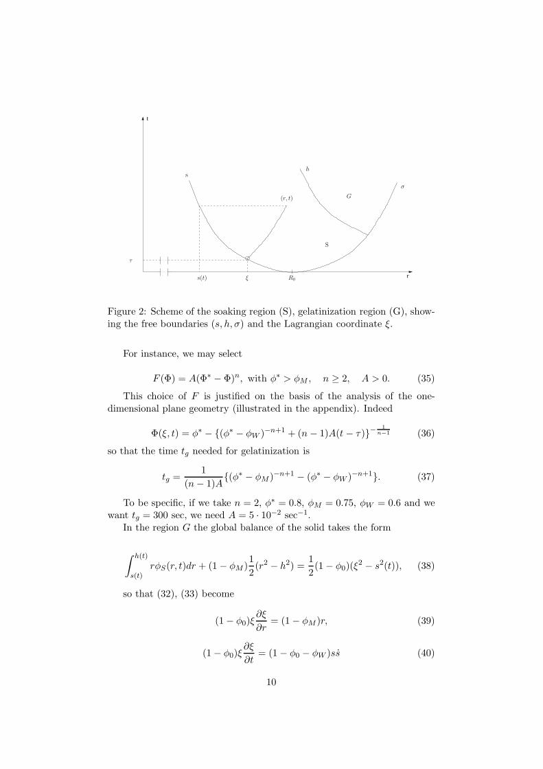
According to the discussion in the previous section, we start at time t = 0with a fully saturated domain 0 < r < R with porosity φ0 << 1; this pristineporosity is introduced for the sake of generality, in view of what said under2(ii), but it could be safely neglected, for practical purposes in the case ofdry pasta. The onset of the soaking process is immediate, while gelatiniza-tion will start only after the porosity has reached some critical value φM .Correspondingly, we have a soaking region S and a gelatinization region G.We consider just a cross section far enough from the ends, exploiting thefact that the ratio radius/length is very small for spaghetti.

2.1 The soaking process.

If we denote by φ the liquid volume fraction and by φS the solid volumefraction, we have that in the region S in which φ ∈ (φ0, φM )

φ + φS = 1. (1)

We describe soaking to be very fast during a first stage, accordinglydescribed as a penetration front accompanied by a jump of φ, then followedby a slower process.

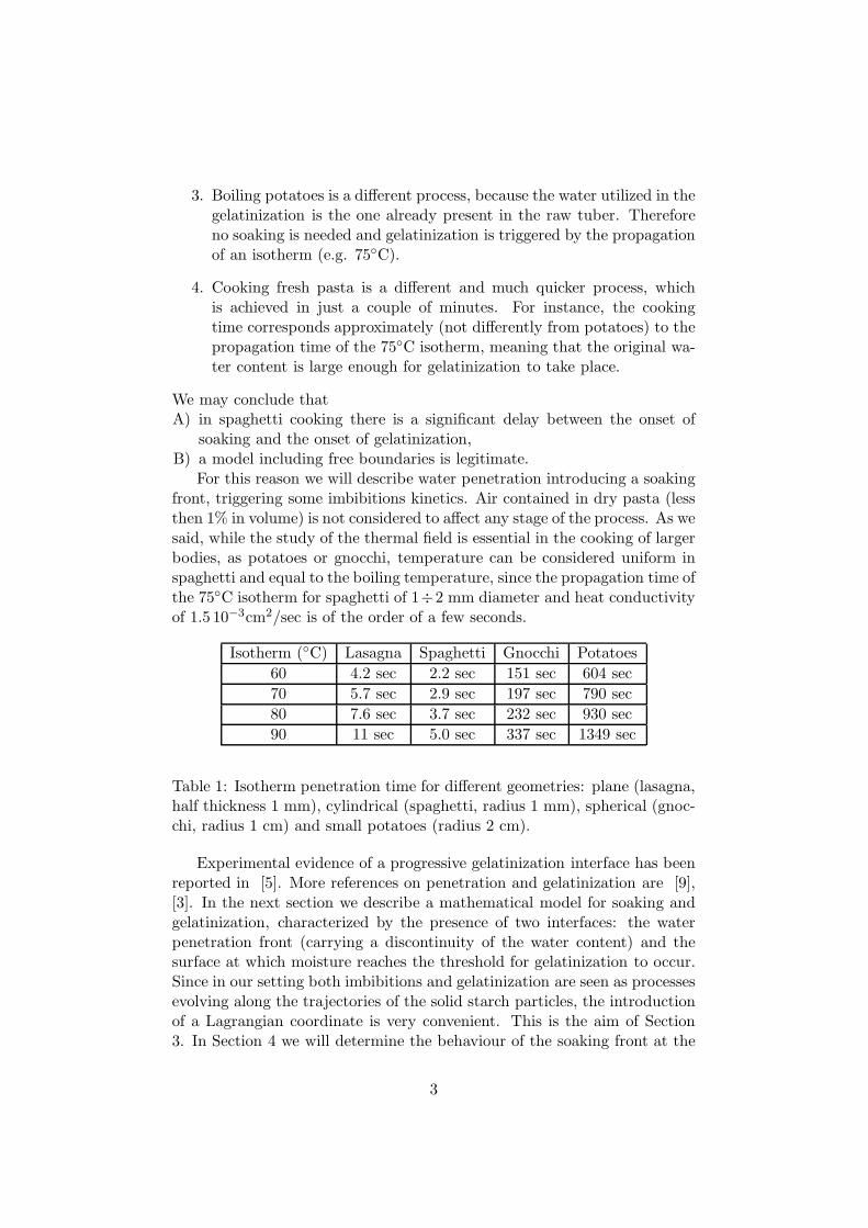
Before the onset of gelatinization, the region S is bounded between twounknown radii: the penetration front r = s(t), and the outer boundary,x = σ(t). The latter will be replaced by the S/G interface r = h(t), fromthe moment it appears (see Fig. 1).

4

Figure 1: Sketch of the geometry of the problem

Instead of using the nonlinear diffusion equation which in the literaturehas been mutuated from the penetration of solvents into glassy polymers,here we describe the residual soaking as a relaxation process, following thekinetics

φ = F (φ), (2)

where φ is the Lagrangian derivative along the motion of the solid particles(the region S moves due to the swelling) and F is positive continuous in [0, 1]and smooth for φ < φM , such that F ′(φ) < 0 for φ ∈ [0, φM ]. Of course Fdepends on the temperature but this is not important here. The selectionof the function F is very delicate. We will discuss some aspects related toit in the Appendix with reference to the problem in a plane geometry.

Denoting by u(r, t) the velocity of the solid particles and by v(r, t) thevelocity of the water, we write the mass balance equation for the two speciesin the region S:

∂φS

∂t+

1

r

∂

∂r(ruφS) = 0, (3)

∂φ

∂t+

1

r

∂

∂r(rvφ) = 0. (4)

Remembering (1) we deduce the global incompressibility condition

∂

∂r[r(uφS + vφ)] = 0. (5)

Now we rewrite (2) in the form

5

∂φ

∂t+ u

∂

∂r(φ) = F (φ), (6)

which, together with (1), (3) yields

φS1

r

∂

∂r(ru) = F (φ). (7)

Similarly we deduce

φ1

r

∂

∂r(rv) = −F (φ). (8)

Finally, Darcy’s law provides the equation for the motion of the waterrelative to the solid:

φ(v − u) = −κ(φ)∂p

∂r, (9)

where κ(φ) is he hydraulic conductivity (also depending on the tempera-ture), and p is pressure. We set the atmospheric pressure equal to zero, andwe impose the conditions

p(σ(t), t) = 0, (10)

p(s(t), t) = −p0, (11)

where p0 is the (temperature dependent) capillary pressure.At the penetration front we suppose that φ jumps from φ0 to a larger

value φW :

φ(s(t)+, t) = φW . (12)

Consistently with the experimental observation that gelatinization seemsto be substantially delayed with respect to soaking, we must assume thatφW is still well below the threshold φM making the onset of gelatinization.

The Rankine-Hugoniot condition associated to (3) reads

[φS ]s = [uφS ] ⇒ (φW − φ0)s(t) = −(1 − φW )u(s(t)+, t), (13)

relating the swelling velocity at the front with the front speed:

u(s(t), t) = −φW − φ0

1 − φWs(t). (14)

The analogous balance for the liquid gives

[φ]s = [vφ] ⇒ (φW − φ0)s(t) = φW v(s(t)+, t), (15)

6

or

v(s(t), t) =φW − φ0

φWs(t) (16)

(of course, if the pristine porosity φ0 is neglected, then the front is a materialsurface, i.e. it moves with the same speed as the water molecules).

We can now observe that the compound velocity φSu + φv evaluatedat the penetration front is zero. Thus (5) implies that it has to vanisheverywhere:

(1 − φ)u + φv = 0. (17)

The initial conditions for the fronts x = σ(t), x = s(t) are obviously

σ(0) = s(0) = R. (18)

Another obvious feature of the soaking model is that s < 0 (the conversewould require water desorption).

As we shall see in the next section (remark 2), the global mass balanceof the solid implies that the external surface moves with the speed u of thesolid particles.

2.2 Gelatinization

It is convenient to model gelatinization as a two-step process, like we havedone for soaking. A first stage fast enough to be considered concentratedat the boundary r = h(t), followed by a second stage evolving according tosome kinetics.

We neglect the possible volume change accompanying the water moleculesrearrangement, since the absence of swelling in boiled potatoes suggests thatgelatinization does not produce any appreciable density change. Since wa-ter is partly immobilized in the gelatinization process, we have to split thewater volume fraction into the sum φ+η of the free and bound components,respectively.

We must impose that

φ + η + φS = 1. (19)

We can write down the balance equation for free and bound water re-spectively

∂φ

∂t+

1

r

∂

∂r(rφv) = −δφS , (20)

∂η

∂t+

1

r

∂

∂r(rηu) = δφS , (21)

where δ represents the transfer rate φ → η per unit volume of the solid. Wemay assume that the process is governed by a known kinetics:

7

δ = G(η) (22)

with G(η) defined for η ∈ [η0, ηM ], positive and smooth for η < ηM , anddecreasing to zero as η → ηM . In our setting η0 is the jump experiencedby η at the interface r = h(t). Of course the model is flexible enough toexclude either the first stage (η0 = 0) or the second stage (η = ηM ). Theratio η/ηM can be considered as an index of gelatinization.

The interface r = h(t) is identified with the level set φ = φM . We remarkthat the continuity of φS across r = h(t) implies the continuity of u:

[φS ] = [u] = 0. (23)

From (19) we have

[φ] = −[η] = −η0, (24)

so the Rankine-Hugoniot condition for (20), gives1

− η0h = (φM − η0)v+ − φMv−. (25)

The r.h.s. of (25) is the difference between the free water fluxes on theright and on the left of the front, while the l.h.s. is the free water loss rateaccompanying the front displacement.

Having neglected any further swelling, we write φS = 0 in the gelatiniza-tion region, implying

φS = 1 − φM , h(t) ≤ r ≤ σ(t) (26)

and ∇ · u = 0, i.e.

ru(r, t) = h(t)u(h(t), t), h(t) ≤ r ≤ σ(t). (27)

Clearly (26) is equivalent to φ + η = φM and therefore the field φv + ηuis divergence free:

r(φv + ηu) = h(t){(φM − η0)v+ + η0u

+}= h(t){φM v− − η0(h − u+)}, h < r < σ, (28)

where we have used (25). Of course (φM − η0)v+ + η0u

+ is the total waterflux.

Darcy’s law has still the form (9) and continuity of pressure is imposedacross r = h(t).

Combining Darcy’s law with (28) (or (25)), we see that across r = h(t)

1From now on we use the obvious notation v± = v(s(t)±, t), u

± = u(s(t)±, t)

8

[

−κ∂p

∂r

]

= η0(u+ − h). (29)

Using the fact that φv + (η + φS)u is divergence free, we easily get, inaddition to (28):

r(φv + (η + φS)u) = −hη0{h − u+}, (30)

owing to the fact that φMv− + (1 − φM )u vanishes.

Remark 1. The problem with η0 = 0 is greatly simplified , since not onlyφS and u are continous across r = h(t), but also φ and v (and consequentlyalso the pressure gradient). In particular (30) provides

φv + (η + φS − 1)u = 0 ⇒ φ(v − u) + u = 0.

3 Describing the motion of solid particles: a La-

grangian coordinate

Let us denote by ξ the radial coordinate of the solid particles at time t = 0,i.e. prior to water penetration with swelling (soaking). This quantity playsthe role of a Lagrangian coordinate during the entire motion. The massconservation of the solid implies that for any (r, t) in the region S

∫ r

s(t)r′φS(r′, t)dr′ =

1

2(1 − φ0)(ξ

2 − s2(t)), s(t) < r < h(t). (31)

Remark 2. Setting r = σ(t) and ξ = R, (31) is shown to be equivalent tou|r=σ = σ.

We can differentiate w.r.t. r and t, obtaining:

(1 − φ0)ξ∂ξ

∂r= rφS , (32)

(1 − φ0)ξ∂ξ

∂t= −rφSu, (33)

compatible with ξ = 0.To the Lagrangian coordinate ξ we may also associate the time variable τ

(Fig. 2), corresponding to the time instant at wich the soaking front reachesthe location ξ:

s(τ) = ξ. (34)

We may transform the unknowns φ(r, t), φS(r, t) to Φ(ξ, t), ΦS(ξ, t), andthis facilitates the integration of equation (2).

9

t

r

s

S

(r, t)

h

G

σ

s(t) ξ R0

τ

Figure 2: Scheme of the soaking region (S), gelatinization region (G), show-ing the free boundaries (s, h, σ) and the Lagrangian coordinate ξ.

For instance, we may select

F (Φ) = A(Φ∗ − Φ)n, with φ∗ > φM , n ≥ 2, A > 0. (35)

This choice of F is justified on the basis of the analysis of the one-dimensional plane geometry (illustrated in the appendix). Indeed

Φ(ξ, t) = φ∗ − {(φ∗ − φW )−n+1 + (n − 1)A(t − τ)}−1

n−1 (36)

so that the time tg needed for gelatinization is

tg =1

(n − 1)A{(φ∗ − φM )−n+1 − (φ∗ − φW )−n+1}. (37)

To be specific, if we take n = 2, φ∗ = 0.8, φM = 0.75, φW = 0.6 and wewant tg = 300 sec, we need A = 5 · 10−2 sec−1.

In the region G the global balance of the solid takes the form

∫ h(t)

s(t)rφS(r, t)dr + (1 − φM )

1

2(r2 − h2) =

1

2(1 − φ0)(ξ

2 − s2(t)), (38)

so that (32), (33) become

(1 − φ0)ξ∂ξ

∂r= (1 − φM )r, (39)

(1 − φ0)ξ∂ξ

∂t= (1 − φ0 − φW )ss (40)

10

We remark that, from (27)

σ(t)σ(t) = h(t)u(h(t), t). (41)

t

tg

R0

Outer Surface

ξ = s(t)

ξ = h(t)

ξ

Figure 3: In the (ξ, t)plane the gelatinization front is just a translation ofthe water penetration front.

The time taken to complete the transition φW → φM is independent ofξ. Thus in the (ξ, t) plane the S/G interface ξ = h(t) is simply obtained bymeans of a time translation of ξ = s(t) by the amount tg (Fig.3):

ξ = h(t) = s(t − tg), t > tg. (42)

The velocity fields in the region S can be found once the function Φ(ξ, t)is known. Note that (32) guarantees that the mapping ξ → r is 1 : 1 foreach t. To find its inverse we can use (32), defining the function

Ψ(ξ, t) =

∫ R

ξ

1 − φ0

1 − Φ(ξ′, t)ξ′dξ′, (43)

which allows to derive from (32) that

r2 = σ2(t) − 2Ψ(ξ, t), t ≤ tg. (44)

At this point, we introduce the transforms U(ξ, t), V (ξ, t), P (ξ, t) ofu(r, t), v(r, t), p(r, t), respectively. Combining (9), (17) and (32), we deduce

U(ξ, t) = k(Φ)r(ξ, t)

ξ

1 − Φ

1 − φ0

∂P

∂ξ. (45)

11

The expression of U(ξ, t) can be found by integrating (7) and recalling(14):

U(ξ, t) =1

r(ξ, t)

{

−φW − φ0

1 − φWss +

∫ ξ

s(t)

(1 − φ0)ξ′

[1 − Φ(ξ′, t)]2F [Φ(ξ′, t)]dξ′

}

, (46)

so that (42) can be used to obtain the pressure field P (ξ, t), exploiting theboundary condition (11).

The fluid velocity field is simply

V (ξ, t) = −1 − Φ

ΦU. (47)

It is interesting to remark that the setting of the soaking model suggeststhat the velocity fields can be found without using Darcy’s law, whose roleseems to be reduced to the determination of the pressure field. In otherwords, pressure looks like to be automatically adjusted to fit the prescribedsoaking kinetics. Nevertheless, pressure is not just an optional quantity.Indeed the motion of the soaking front has still to be determined and to thisaim it is necessary to use the boundary condition (11), so that Darcy’s lawfully comes into play.

Returning to the original variables, the velocity field u(r, t) becomes

u(r, t) =1

r

{

−φW − φ0

φWss +

∫ r

s

r′

1 − φ(r′, t)F [φ(r′, t)]dr′

}

(48)

and we may write

p0 =

∫ σ(t)

s(t)

u(r, t)

k[φ(r, t)]dr, (49)

to be interpreted as a functional equation for s(t), since in turn the boundaryσ(t) is implicitly defined putting ξ = R in (31):

∫ σ(t)

s(t)r[1 − φ(ξ, t)]dr =

1

2(1 − φ0)(R

2 − s2(t)). (50)

Since 1 − φ < 1 − φ0, (50) has a unique solution σ(t) > R, ∀t > 0. Thesystem (49), (50) is more complicated than it looks, since we must rememberthat φ depends explicitly on the time τ , and through it on s. We remindthat it has to be used in the stage preceding gelatinization.

After the appearence of the region G, as we have seen, the relationshipbetween r and ξ is more complicated. On the basis of (38) and (31) wededuce that in G the inverse mapping ξ → r can be expressed as

σ2 − r2 =1 − φ0

1 − φM(R2 − ξ2), h(t) ≤ ξ ≤ R, (51)

12

where ξ = h(t) corresponds to r = h(t), namely

h(t)2 = R2 − 1 − φM

1 − φ0(σ2 − h2). (52)

For ξ < h, we have instead

h2 − r2 = 2

∫ h(t)

ξ

1 − φ0

1 − Φ(ξ′, t)ξ′dξ′, t > tg. (53)

As we have pointed out, the curve ξ = h(t) is nothing but ξ = s(t − tg)for t > tg. Thus (52) can be used as the formula giving h(t) in terms of σ(t)and of s(t − tg), for t > tg.

4 A-priori properties of the water penetration front

We can easily deduce the behaviour of s(t) and σ(t) for small t, takingthe approximation φ ∼ φW in (49) and (50). First of all we deduce theasymptotic relationship:

σ2(t) ≈ 1

1 − φW[(1 − φ0)R

2 − (φW − φ0)s(t)2], (54)

or, to the first order in σ − R or R − s,

σ − R ≈ φW − φ0

1 − φW(R − s). (55)

Clearly, since σ − s ≈ 1−φ0

1−φW(R − s), in order to satisfy (49), u must

exhibit a singularity of the order 1R−s , which in (48) can only be attributed

to s. Hence, if we want −s = ddt(R − s) to behave as (R − s)−1, we must

take the ansatz:

s(t) ≃ R(1 − α√

t) ⇒ σ(t) ≃ R

(

1 +φW − φ0

1 − φWα√

t

)

(56)

and we can keep just the singular term of u to perform the calculation in(49), obtaining the coefficient α:

α =

[

2k(φW )p0

(φW − φ0)(1 − φ0)

]1/2 1 − φW

R. (57)

The soaking processes is related to the efficiency of water transport,besides the intensity of the capillarity (expressed by p0). Indeed, couplingthe equations u = k∇p and div(u) = F/φS , we see that pressure satisfiesthe elliptic equation

13

div(k(φ)∇p) =F (φ)

1 − φ, s(t) < r < σ(t). (58)

Using the expression (14) of u on the soaking front, we get the Stefancondition

− φW − φ0

1 − φSs = k(φW )

∂p

∂r|r=s(t). (59)

The quantity

β = k(φW )∂p

∂r|r=s(t) (60)

can be calculated integrating twice (58) and imposing the two boundaryconditions for pressure:

β

∫ σ

s

dr

k(φ)= p0 −

∫ σ

s

1

k(φ)

(∫ r

s

r′F

1 − φdr′

)

dr, (61)

leading to the estimate

β <p0kmax

σ − s− Fmin

1 − φW

σ2 − s2 + s(σ − s)

6(62)

Using the inequalities (see (50))

(σ2 − s2)(1 − φM ) < (1 − φ0)(R2 − s2) < (σ2 − s2)(1 − φW ), (63)

it is possible to derive from (60), (62) a differential inequality for s.

5 Study of the water penetration stage

Going back to equation (2), we immediately realize that, introducing thefunction

Q(y) =

∫ y

φW

dz

F (z)(64)

we obtain the integral

Φ(ξ, t) = Z(t − τ(ξ)), (65)

with Z = Q−1, emphasising the dependence on the difference t − τ(ξ). Theuse of the Lagrangian variable ξ seems more natural if we want to studyequation (49). Once more, from (32)

dr =1 − φ0

1 − φ

ξ

r(ξ, t)dξ for fixed t,

14

and we can write (46) as

p0 =

∫ R

s(t)

U(ξ, t)

k(Φ(ξ, t))

1 − φ0

1 − Φ(ξ, t)

ξ

r(ξ, t)dξ, (66)

where U(ξ, t) is given by (46), Φ by (65) and r(ξ, t) by (43) and (44).Hence

p0 = −(1 − φ0)(φW − φ0)

1 − φWs(t)s(t)

∫ R

s(t)

ξdξ

r2k(Φ)(1 − Φ)+

+(1 − φ0)2

∫ R

s(t)

ξdξ

r2k(Φ)(1 − Φ)

∫ ξ

s(t)

ξ′

[1 − Φ(ξ′, t)]2F [Φ(ξ′, t)]dξ′.(67)

It is now convenient to use the transformation ξ = s(τ), ξ′ = s(τ ′):

p0 =(1 − φ0)(φW − φ0)

1 − φWs(t)s(t)

∫ t

0

s(τ)s(τ)dτ

r2k[Z(t − τ)][1 − Z(t − τ)]+

+ (1 − φ0)2

∫ t

0

{

s(τ)s(τ)dτ

r2k[Z(t − τ)][1 − Z(t − τ)]·

·∫ t

τ

s(τ ′)s(τ ′)

[1 − Z(t − τ ′)]2F [Z(t − τ ′)]dτ ′

}

dτ (68)

where (after the usual transformation in (44))

r2(s(τ), t) = σ2(t) + 2

∫ τ

0

1 − φ0

1 − Z(t − τ ′)s(τ ′)s(τ ′)dτ ′ (69)

and σ(t) is expressed through s(t) by means of

σ(t) = R +

∫ t

0U(R, τ)dτ, (70)

namely (see 46)

σ(t) = R +

∫ t

0

1

σ(τ)

{

−φW − φ0

1 − φWs(τ)s(τ)−

−∫ τ

0

(1 − φ0)s(τ′)s(τ ′)

[1 − Z(t − τ ′)]2F [Z(t − τ ′)]dτ ′

}

dτ, (71)

i.e. a nonlinear Volterra integral equation, with the product ss entering thekernel (which is weakly singular).

Therefore the r.h.s. of (68) can be regarded as an operator applied tothe product ss.

Now we prove the following

15

Theorem 5.1. The functional equation (68) has a unique solution s(t),continuously differentiable for t > 0 and continuous for t = 0.

Proof. Let us define

− ss√

t = Σ(t), (72)

and

B(t, τ ; Σ) =

∫ t

τ

Σ(τ ′)√τ ′

dτ ′

r2(s(τ ′), t)k[Z(t − τ ′)][1 − Z(t − τ ′)], (73)

where r2 is defined in terms of Σ via (69), (71), (72).We may rewrite equation (68), using the quantities above and inter-

changing the order of integration in the double integral:

p0 =(1 − φ0)(φW − φ0)

1 − φWΣ(t)

1√tB(t, 0;Σ) +

+ (1 − φ0)2

∫ t

0

Σ(τ)√τ

F [Z(t − τ)]

[1 − Z(t − τ)]2B(t, τ ; Σ)dτ (74)

We consider the set

S =

{

Ξ ∈ C[0, T ]| Ξ(0) =1

2αR2, 0 < µ0 ≤ Ξ ≤ µ1

}

, (75)

where T , µ0, µ1 are parameters to be chosen (more restrictions will beimposed in the course of the proof).

Taken Ξ ∈ S, we use it to compute B(t, τ ; Ξ), according to (73), with Ξreplacing Σ also in (69), (71), and we define the mapping M : Ξ 7−→ Σ bymeans of the Volterra equation

p0 =(1 − φ0)(φW − φ0)

1 − φWΣ(t)

1√tB(t, 0; Ξ) +

+ (1 − φ0)2

∫ t

0

Σ(τ)√τ

F [Z(t − τ)]

[1 − Z(t − τ)]2B(t, τ ; Ξ)dτ (76)

(whose solvability is immediately established by means of a contractive map-ping argument). Note that t−1/2B(t, 0; Ξ) is uniformly bounded for ξ ∈ S ifwe restrict T in such a way that r, as given by (69), is greater than a givenfraction of R, i.e. R/N with N > 1. For instance, a rough estimate of suchtime TN can be

R2

N2≤ R2 − 2

∫ TN

0

1 − φ0

1 − φM

µ1√τdτ,

16

hence

TN ≤[

R2

4µ1

(

1 − 1

N2

)

1 − φM

1 − φ0

]2

, (77)

implying that, for t ∈ (0, TN ),

1√tB(t, 0; Ξ) <

2µN2

R2kmin(1 − φM )=: BM . (78)

We can also say that t−1/2B(t, 0; Ξ) is uniformly bounded away fromzero, since

1√tB(t, 0; Ξ) >

µ0√t

∫ t

0

1

R2kmax

1√τdτ =

2µ0

R2kmax=: Bm. (79)

Coming back to equation (76), since both terms on the r.h.s. are positive,we can derive the following estimates:

Σ(t) <p0(1 − φW )

(1 − φ0)(φW − φ0)

R2kmax

2µ0, (80)

Σ(t) >p0(1 − φW )

(1 − φ0)(φW − φ0)

R2kmin(1 − φM )

2µ1N2− (1 − φ0)

2

1 − φMFmax2t sup

[0.T ]Σ(t)

(81)so we can possibly reduce T so to guarantee that Σ(t) is greater than a givenfraction of Σ(0).

Unfortunately, (80), (81) just say that Σ is bounded, but they are un-suitable to show that M maps S into itself.

Therefore, let us take the subset S ⊂ S in which we impose the furtherrequirement that Ξ is Lipschitz continuous in any interval [ε, T ], with ε > 0and Lipschitz constant L(ε), unbounded for ε → 0 and decreasing in ε.

Since we will prove that the limit Σ(t) → Σ(0) as t → 0+ is uniformfor Ξ in S, the structure we have given to S guarantees the existence of afixed point of the mapping M, using Schauder’s theorem in a suitable way,provided we prove that MS ⊂ S and that M is continuous in S w.r.t. thesup norm.

With this aim, and keeping in mind all the restrictions we have imposedon T , let us compute the difference Σ(t1) − Σ(t2), e.g. with t1 > t2. From(76), setting:

a = (1−φ0)(1−φW )φW −φ0

, F(Z) = F (Z)(1−Z)2

, ‖Σ‖ = sup(0,T ) Σ(τ)

K(Z) = [k(Z)(1 − Z)]−1, F∗ = supZ∈(0,φM ) |F ′|, K∗ = supZ∈(0,φM ) |K′|,

FM = supy∈(0,φM ) F (y), 0 < Bm = inf B√t

for any Ξ ∈ S,

17

we get

|Σ(t1) − Σ(t2)| ≤ ‖Σ‖∥

∥

∥

∥

1√t1

B(t2, 0; Ξ) − 1√t2

B(t2, 0; Ξ)

∥

∥

∥

∥

+

+a

Bm

∥

∥

∥

∥

∫ t2

0

Σ(τ)√τ

F ′(Z)[Z(t1 − τ) − Z(t2 − τ)]B(t1, τ ; Ξ)dτ

+

∫ t2

0F(Z(t2 − τ))[B(t1, τ ; Ξ) − B(t2, τ ; Ξ)]dτ

∥

∥

∥

∥

+

+a

Bm

∫ t2

t1

Σ(τ)√τF(Z(t1 − τ))B(t1, τ ; Ξ)dτ,

(82)

with t1 > t2 > ε.Using the estimates

|σ(t1) − σ(t2)| ≤µ1

R

φW − φ0

1 − φW

1

2√

t2(t1 − t2) (83)

(deducible from (71), for T sufficiently small)

|r2(s(τ), t1) − r2(s(τ), t2)| ≤ µ1φW − φ0

1 − φW

1√t2

(t1 − t2)+

+ 4(1 − φ0)µ11

(1 − φM )2FM (t1 − t2)

√τ ,

(84)

(deducible from (69)) we get the inequality

∣

∣

∣

∣

1√t1

B(t1, 0; Ξ) − 1√t2

B(t2, 0; Ξ)

∣

∣

∣

∣

≤ Cµ1t1 − t2

t2, t1 > t2 > ε, (85)

valid for T sufficiently small and a suitable constant C, independent on T ,µ1. The other terms in (82) are less important, due to the presence of theintegral, so we can say that

|Σ(t1) − Σ(t2)| ≤ C‖Σ‖µ1t1 − t2

t2, t1 > t2 > ε, (86)

for some other constant C.Now we can use the estimate (80) for ‖Σ‖ to derive the expression of

L(ε) in terms of µ1. The above estimate is too crude near the origin becauseit cumulates singularities that instead should cancel. Therefore the analysisnear t = 0 should be performed more carefully.

We are just interested in the lowest order of the increment. Let us addone more restriction to the set of functions Ξ, requiring that

|Ξ(t) − Ξ(0)| ≤ λ√

t, (87)

18

where λ must be established so that the same inequality is true for thefunction Σ(t) = MΞ.

The difference Σ(t)−Σ(0) can be evaluated directly from (76). We realiseimmediately that

Σ(t)1√tB(t, 0; Ξ) − Σ(0)C = O(t), (88)

where

C = limt→0

B√t

=2Σ(0)

R2k(φW )(1 − φW ).

Since we are interested in the√

t term only, we may say that

|Σ(t) − Σ(0)| ≈ 1

C

∣

∣

∣

∣

1√tB(t, 0; Ξ) − C

∣

∣

∣

∣

Σ(t). (89)

On the right hand side we may replace Σ(t) by Σ(0), once we havechecked that Σ(t) − Σ(0) = O(

√t).

Let us now compute:

∣

∣

∣

∣

1√tB(t, 0; Ξ) − C

∣

∣

∣

∣

=1√t

∣

∣

∣

∣

∫ t

0

1√τ

{

Ξ(τ)

r2k(Z)(1 − Z)− Ξ(0)

R2k(φW )(1 − φW )

}

dτ

∣

∣

∣

∣

≤

≤ Σ(0)√t

∫ t

0

1√τ

∣

∣

∣

∣

1

r2k(Z)(1 − Z)− 1

R2k(φW )(1 − φW )

∣

∣

∣

∣

dτ +

+λ√t

∫ t

0

dτ

r2k(Z)(1 − Z).

Neglecting some O(t) terms, the last member of the above inequality is

1

R2k(φW )(1 − φW )

{

Σ(0)√t

∫ t

0

1√t

|R2 − r2|R2

dτ + λ√

t

}

From (69) and (71) we see that

r2(s(t), t) − R2 = 2R

∫ t

0U(R, τ)dτ − 2

∫ t

0

1 − φ0

1 − Z

Ξ(τ ′

τ ′ dτ ′

with

∫ t

0U(R, τ)dτ = 2

Σ(0)

R

φW − φ0

1 − φW

√t + O(t).

Therefore after some algebra we obtain that

r2(s(t), t) − R2 = −4Σ(0)√

t + O(t).

19

Summing up the above results and remembering that

Σ(0)

C=

R2k(φW )(1 − φW )

2,

we reach the conclusion

|Σ(t) − Σ(0)| ≈{

4Σ(0)

R2+ λ

}√t

=

(

α +1

2λ

)√t. (90)

Therefore Σ(t) satisfies the same inequality (87) as Ξ(t) provided thatα + λ/2 ≤ λ, meaning that we have simply to choose λ ≥ 2α.

It is worth nothing that λ can now be selected independently of theother parameters entering the definition of the set S, thus providing uniformbounds for Ξ for some other interval Tλ. Since the O(t) terms depend onµ1, the length of this time interval may depend on µ1.

From what we have seen, we want in practice that λ√

Tλ > Cµ1Tλ, forsome C independent of µ1, implying that Tλ < (λ/Cµ1)

2. We may chooseµ1 = 2Σ(0) = αR2. Next, using the Lipschitz estimate we can look for atime T1 > Tλ such that over (Tλ, T1), Σ(t) has a further decrement less thanΣ(0): 3Σ(0)C1(T1 − Tλ)T−1

λ < Σ(0), for a suitable C1 independent of ‖Σ‖.Thus we find (T1 − Tλ)t−1

λ < (3C1)−1. Allowing a further decrement not

exceeding Σ(0), we can look for T2 such that 4Σ(0)C1(T2 − T1)T−11 < Σ(0),

i.e. (t2 − T1)T−11 < (4C1)

−1. Continuing this procedure, we may say thatΣ(t) < (n + 2)Σ(0) for t < Tn = Πn

j=3(1 + (jC1)−1)Tλ.

In this way, we may select µ1 and T (and consequently µ0 and L(ε)), i.e.all the parameters in the set S, so to guarantee that MS ⊂ S.

Let’s turn our attention to the continuity of M. This is easy, since from(69), (71), (73) (76) we obtain the estimate

‖Σ1 − Σ2‖ ≤ X√

T‖Ξ1 − Ξ2‖, (91)

where X is a constant depending on the parameters defining S. Thus M isnot only Lipschitz continous, but even contractive for T small enough.

Remark 3. Existence and uniqueness can be easily extended up to the timetg at which φ reaches ΦM and that we suppose to be such that s(tg) > 0.Indeed in practical cases gelatinization has to start much before water reachesthe axis.

6 Study of the gelification stage.

For the sake of brevity we confine to the case η0 = 0, characterized by thecontinuity of all quantities through the interface r = h(t).

20

Recalling (30), we see that the equation

k(φ)∂p

∂r= u

extends in the region G. Consequently, equation (49) is still valid.Concerning the link between σ(t) and s(t), we see from (42), (51) and

(53) that it can be written as

σ2(t) − s2(t) = 2

∫ R

s(t)

1 − φ0

1 − Φ(ξ, t)ξdξ, (92)

where

Φ(ξ, t) =

{

Φ(ξ, t), s(t) ≤ ξ ≤ h(t)

φM , h(t) ≤ ξ ≤ R.(93)

We recall that h(t) = s(t− tg), so that (92) really provides the mappings → σ.

The expression of the velocity field u(r, t) is

ru(r, t) = −φW − φ0

1 − φWss +

∫ r

s

r′

1 − φ(r′, t)F (φ(r′, t))dr′, s ≤ r ≤ h, (94)

as before, and

ru(r, t) = −φW − φ0

1 − φWss +

∫ h

s

r

1 − Φ(r, t)F (φ(r))dr, h ≤ r ≤ σ, (95)

owing to (27). Remembering (44), we have that (95) is also the expressionof σσ.

It is advantageous to use the Lagrangian variable ξ because the functionφ(r, t) has a simpler expression. We just have to modify the definition (65)of Φ(ξ, t) as follows,

Φ(ξ, t) =

{

Z(t − τ(ξ)), ξ ≤ h(t)

φM , ξ ≥ h(t).(96)

In this way we can write the explicit form of the functional equation forthe free boundary s(t) and we realise that it is formally identical to the oneof the soaking stage with the only change that Φ is defined as in (96) andF (Φ) is consequently frozen to zero in the gelatinization region.

Therefore the existence proof is very similar to the one illustrated indetail in sect. 5.

21

7 A numerical scheme

We recall that (56), (57) give a good representation of s(t), σ(t) for t <<α−2. Thus, we select a partition

(0, tg) = ∪N−1i=1 (ti, ti+1)

with t0 = 0, t1 << α−2, TN = tg, and we identify s(t), σ(t) with theirapproximations (56) in the first interval (0, t1), which we call s0(t), σ0(t):

s0(t) = R(1 − α√

t), σ0(t) = R

(

1 +φW − φ0

1 − φWα√

t

)

. (97)

According to (69), the corresponding O(√

t) approximation of ε2 for0 < τ < t < t1 is

r2 ≈ σ20(t) −

1 − φ0

1 − φW(R2 − s2

0(τ))

≈ R2

{

1 +rα

1 − φW[(φW − φ0)

√t − (1 − φ0)

√τ ]

}

,

(98)

where we have used the approximation Z ≈ φW .Before we proceed further, it is convenient to take nondimensional vari-

ables, rescaling lengths by R (r = rR, s = sR, σ = σR) and time by

t0 = α−2, so that α√

t =√

t, α√

τ =√

τ . We rescale k by kW = k(φW ) andwe introduce the nondimensional quantity

Θ = Aα−2 (99)

(note that Θ is the ratio between the time scale α−2 associated with thefront penetration and the time scale A−1 associated to the soaking kinetics).Moreover, we write

s(t)ds

dt= − S(t)

2√

t.

Remembering (57) we can now write the non-dimensional form of (68) inthe following form, where all tildes have been omitted to simplify notations:

1 =S(t)√

t

∫ t

0

1

r2

S(τ)

2√

τ

1

k[Z(t − τ)]

1 − φW

1 − Z(t − τ)dτ+

+ 2Θ1 − φ0

φW − φ0

∫ t

0

{

S(τ)

r√

τ

1

r2

1

k[Z(t − τ)]

1 − φW

1 − Z(t − τ)·

·∫ t

τ

S(τ ′)

2√

τ ′[φ∗ − Z(t − τ ′)]2

1 − φW

[1 − Z(t − τ)]2dτ ′

}

dτ

(100)

Note that we have specified n = 2 in (100).

22

In the new variable, starting from s0 = 1−√

t we define S0 = 1−√

t andwe may decide to approximate S(t) in (t1, t2) by the constant S1 obtainedfrom (100) taking t = t1, S(t) = S1 and keeping just the approximationO(

√t1):

S1 ≈ 1 +

(

1

2+ 2

φW − φ0

1 − φ0− 1 − φ0

2

)√t1, (101)

where we have used the nondimensional approximations

σ0(t) ≈ 1 +φW − φ0

1 − φW

√t, (102)

r2 ≈ 1 + 2φW − φ0

1 − φWt − 2

1 − φ0

1 − φW

√τ . (103)

We can proceed in a recursive way to derive a constant approximationfor S(t), that we call sn, in the interval (tn, tn+1).

To this end we need the non-dimensional version of (69), (71), namely(with a slight abuse of notation)

r2(τ, t) = σ2(t) − (1 − φ0)

∫ τ

0

S(τ ′)√τ ′

1

1 − Z(t − τ ′)dτ ′, (104)

σ = 1 +

∫ t

0

1

σ(τ)

{

φW − φ0

1 − φW

S(τ)

2√

τ+

+ Θ

∫ τ

0

1 − φ0

1 − Z

S(τ ′)

2√

τ ′

[φ∗ − Z(t − τ ′)]

1 − Z(t − τ ′)dτ ′

}

dτ

(105)

The recursive system for the determination of the triples (Sn, rn, σn) isthe following

1 = Sn

n−1∑

i=0

Si

r2i,n

1

ki

1 − φW

1 − Zi,n

√ti+1 −

√ti√

tn+

+ 2Θ1 − φ0

φW − φ0

n−1∑

i=0

Si

r2i,n

1

ki

1 − φW

1 − Zi,n(√

ti+1 −√

ti)·

·

n−1∑

j=i

Sj1 − φW

1 − Zj,n(φ∗ − Zj, n)2(

√

tj+1 −√

tj)

(106)

where Zi,n = Z(tn − ti),

r2i,n = σn − (1 − φ0)

i−1∑

j=0

Sj1

1 − Zj,n(√

tj+1 −√

tj), (107)

23

σn = 1 + (√

ti+1 −√

ti)

{

n−1∑

i0

Si

σi

φW − φ0

1 − φW(√

ti+1 −√

ti)+

+(1 − φ0)Θn−1∑

i=0

1

σi

i−1∑

j=0

Sj

1 − Zj,n

[φ∗ − Zj,n]2

1 − Zj,n(√

tj+1 −√

tj)

.

(108)

Once (106-108) has been solved, the approximations sn are obtained via

sn =

{

R2 − 2

n−1∑

i=0

Si(√

ti+1 −√

ti)

}

1

2

. (109)

8 Comparison with experiments

In [1] measures of total water intake are reported with reference to severaldifferent geometries.

Using the asymptotic analysis of Section 4, we deduce the total waterintake during the first stage of the process, during which the progressionof the water penetration front has the behaviour s(t) ≈ R − α

√t, we can

easily calculate the total water intake as a function of time. Indeed, from(56) we deduce a simple expression for σ(t), s(t). To be consistent with thisapproximation, we take φ ≈ φW and we just neglect the pristine porosity φ0

which is very small.The volume of water present in the sample at time t is π[σ2(t) − s2(t)].

Thus, taking into account (56), (57) (with φ0 = 0), the mass of wateruptaken per unit length, computed at the O(

√t) order, is

M(t) = 2πRρWα

1 − φW

√t, (110)

where ρW is the water density and α is given by (57).The same quantity, divided by the mass of pasta per unit length, i.e.

πρstarchR2, is plotted in Fig. 4, in which the experimental data from [1] areshown. The fitting of the coefficient

a = 2ρW

ρstarch

φW

R

α

1 − φW

by the least sqares method gives a = 0.048 sec−1/2.Taking φW = 0.35, ρW = 1g cm−3, ρstarch = 1.4g cm−3 (as in [6]),

and R = 0.07cm (as in [1]), this value of a corresponds to p0kW ≈ 7.6 ·10−6cm2sec−1, which in our scheme is the driving quantity.

We took advantage of the fact that in [1] there also the water intakeresults for plane geometry and we perform tha same data fitting procedure,

24

0 100 200 300 400 5000

0.2

0.4

0.6

0.8

1

1.2

1.4

Figure 4: Early stage of water penetration in cylindrical symmetry(spaghetti) vs. experimental data

0 200 400 600 800 10000

0.5

1

1.5

2

2.5

Figure 5: Early stage of water penetration in plane symmetry (lasagna) vs.experimental data

25

this time based on the formula (see the Appendix, formula (113), and con-sider that −σ ≈ φW

1−φWs)

M(t) = ρWφ

1 − φWα√

t, α = (1 − φW )

√

2p0kW

φW.

The quantity to be compared with the data is M(t)ρstarchL , L being the half

thickness of the sample (L = 0.025cm). The value identified for the coeffi-cient of

√t is a = 0.07sec−1/2, corresponding to p0kW = 1.5 · 10−6cm sec−1,

which is not much different from the previous one (see Fig. 4). Part of thediscrepancy could be attributed to the longitudinal expansion of spaghetti,which has been neglected here, but also to very small thickness of the flatpasta sample that has been used.

Appendix. Plane geometry and qualitative remarks

We deal briefly with the case of plane geometry with the main scope ofemphasizing the influence of some parameters on the soaking process, takingadvantage of the much simpler structure of the equations. The problemwith a plane geometry has a practical interest, as we pointed out in theintroduction.

Confining to the water invasion stage, we choose the space coordinatex so that the moisturised region is σ(t) < 0 < x < s(t), for t > 0, andσ(0) = s(0) = 0. We keep all other symbols used so far, and in particularthe form (35) of the function determining the soaking kinetics:

φ = A(φ∗ − φ)n, φ∗ ≥ φM , n > 0, A > 0. (111)

We want to examine the influence of the exponent n, here allowed to beany positive number.

The equation replacing (68) turns out to be

p0 =(1 − φ0)(φW − φ0)

1 − φWs(t)

∫ t

0

s(τ)

k[Z(t − τ)][1 − Z(t − τ)]dτ+

+ (1 − φ0)2A

∫ t

0

s(τ)

k[Z(t − τ)][1 − Z(t − τ)]

∫ t

τ

[φ∗ − Z(t − τ ′)]n

[1 − Z(t − τ ′)]2s(τ ′)dτ ′dτ,

(112)

which again gives a singular asymptotic behaviour for small time:

s(t) ≈ αt1

2 , α =

√

2(1 − φW )2k(φW )

(φW − φ0)(1 − φ0)p0 (113)

(see Fig. 5).

26

Equation (112) is much simpler than equation (68) because the latterinvolved also the function r(ξ, t) and consequently also σ(t). Therefore theargument used to prove existence for equation (68) applies to (112) too withgreat simplifications.

Numerical computations performed on (112) show that a non-monotonebehaviour for s(t) is possible for n ≤ 1. A possible inversion of the frontmotion, although not expected in practice, fits the physics of the model.Indeed we have assumed that, while water is driven in the medium by cap-illarity, it is also required to feed the imbibition process at each point. Theneed of water required by the latter may not be matched by the transportmechanism (which is Darcyan in our scheme). When this happens water canbe forced to invert its motion. Of course this is not the kind of behaviourwe expect for pasta cooking and we must select the parameter so to guar-antee monotonicity. A crucial parameter is the exponent n in the kineticsof imbibition. Taking n < 1 accelerates imbibition to the point that a frontregression can be induced.

In order to have an idea of how the selection of n influences the solutionwe can argues as follows. Put ω(t) = s(t) in (112) and suppose that ω(t)vanishes for the first time at some instant t > 0. If we differentiate (112)w.r.t. t and we take t = t, thanks to the fact ω(t) = 0 and ω(t) ≤ 0, weobtain

0 = Θ1 + Θ2,

where Θ1, Θ2 come from the differentiation of the first and of the secondterm on the r.h.s., respectively. It is easily seen that Θ1 ≤ 0, thanks toω(t) ≤ 0 and to ω(t) = 0 in t.

Therefore, if we want to contradict the assumption ω(t) = 0, we needΘ2 < 0.

Consider for simplicity the case k = constant . The computation of Θ2

leads to

kΘ2

(1 − φ0)2=

∫ t

0

ω(τ)

[1 − Ψ(t − τ ]2Ψ(t − τ)

∫ t

τ

[φ∗ − Ψ(t − τ ′)]n

[1 − Ψ(t − τ ′)]2ω(τ ′)dτ ′dτ+

+

∫ t

0

ω(τ)

[1 − Ψ(t − τ)]·

{

∫ t

τ

Ψ(t − τ ′)[φ∗ − Ψ(t − τ ′)]n−1

[1 − Ψ(t − τ ′)]3[

−n(1 − Ψ(t − τ ′) + 2(φ∗ − Ψ(t − τ ′)))]

dτ ′

}

dτ

(114)

This formula emphasizes that a necessary condition for Θ2 < 0 is that

n

2>

φ∗ − Z

1 − Z.

27

For Z ∈ (φW , φM ) we have

φ∗ − φM

1 − φM<

φ∗ − Z

1 − Z<

φ∗ − φW

1 − φW< 1.

Although this is not a conclusive argument, it suggests that acceptable valuesfor n are in the range n ≥ 2.

From (112) we can also obtain an indication of how the coefficient Ainfluences the solution. Setting ωA= ∂ω

∂A, by differentiation w.r.t. A we obtain

0 =φW − φ0

1 − φW

{

ωA(t)

∫ t

0

ω(τ)

k(Z)(1 − Z)dτ + ω(t)

∫ t

0

ωA(t)

k(Z)(1 − Z)dτ

}

+

+ (1 − φ0)

∫ t

0

ω(τ)

k(Z)(1 − Z)

{∫ t

τ

(φ∗ − Z)n

(1 − Z)2ω(τ ′)dτ ′+

+A

∫ t

τ

(φ∗ − Z)n

(1 − Z)2ωA(τ ′)dτ ′

}

dτ+

+ (1 − φ0)A

∫ t

0

ωA(τ)

k(Z)(1 − Z)

∫ t

τ

(φ∗ − Z)n

(1 − Z)2ω(τ ′)dτ ′dτ.

(115)

This is a linear integral equation in ωA, which allows to conclude thatωA < 0 as long as ω > 0.

The physical implication is that increasing the coefficient A (i.e. thatlocal imbibition rate) reduces the front speed. Indeed, as we said, the twoprocesses are in mutual competition.

In the same way it is possible to show the following. If we write k(Z) =k0k(Z) and we investigate the dependence of ω on k0, we conclude that ωincreases if k0 increases. The results agrees with physical intuition, sinceenhancing the water transport accelerates the front penetration.

References

[1] S. Cafieri, S. Chillo, M. Mastromatteo, N. Suriano and M. A. Del NobileA mathematical model to predict the effect of shape on pasta hydrationkinetic during cooking and overcooking, J. Cereal Science, (2008)

[2] E. Cocci, G. Sacchetti, M. Vallicelli and M. Dalla Rosa Spaghetticooking b microwave oven: cooking kinetics and product quality, J.Food Eng., 85 (2008), 537–546.

[3] S. E. Cunningham, W. A. M. Mcminn, T. R. A. Magee and P. S.Richardson Modelling water absorption of pasta during soaking, J.Food. Eng., 82 (2007), 600–607.

28

[4] M. J. Davey, K. A. Landman, M. J. McGuinness and H. N. Jin Math-ematical modelling of rice cooking and dissolution in beer production,AIChE Journal, 48(2002), 1811–1826.

[5] R. A. Grzybowski and B. J. Donnelly Starch gelatinization in cookedspaghetti, J. Food Science, 42 (1977), 1304–1315.

[6] M. J. McGuinness, C. P. Please, N. Fowkes, P. McGowan, L. Ryderand D. Forte Modelling the wetting and cooking of a single cereal grain,IMA J. Math. Appl. Business and Industry, 11 (2000), 49–70.

[7] A. G. F. Stapley, P. J. Fryer and L. F. Gladden Diffusion and reactionin whole wheat grains during boiling, AIChE Journal, 44 (1998), 1777–1789.

[8] A. K. Syarief, R. J. Gustafson and R. V. Morey Moisture diffusioncoefficients for yellow-dent corn components, Trans. ASAE, 30 (1987),522–528.

[9] Ch. Xue, N. Sakai and M. Fukuoka Use of microwave heating to controlthe degree of starch geletinization in noodles, J. Food. Eng., 87 (2007),357–362.

[10] Tain-Yi Zhang, A. S. Bakshi, R. J. Gustafson and D. B. Lund Finiteelement analysis of nonlinear water diffusion during rice soaking, J.Food Science, 49 (1984), 246–277.

29