Journal of

Marine Science and Engineering

Article

A Mesh Deformation Method for CFD-Based Hullform Optimization

Kwang-Leol Jeong 1 and Se-Min Jeong 2,*1 Research Center, NEXTfoam Co., Ltd., Seoul 08512, Korea; kl.jeong@nextfoam.co.kr2 Department of Naval Architecture and Ocean Engineering, Chosun University, Gwangju 61452, Korea* Correspondence: smjeong@chosun.ac.kr; Tel.: +82-62-230-7218

Received: 8 June 2020; Accepted: 24 June 2020; Published: 26 June 2020�����������������

Abstract: Computational fluid dynamics (CFD) is an effective tool for ship resistance predictionand hull form optimization. A three-dimensional volume mesh is essential for CFD simulation,and mesh generation requires much time and effort. Mesh deformation can reduce the time formesh generation and simulation. The radial basis function (RBF) and inverse distance weighted(IDW) methods are well-known mesh deformation methods. In this study, the two methods arecompared and a novel mesh deformation method for hull form optimization is proposed. For thecomparison, a circular cylinder polyhedral mesh was deformed to the National Advisory Committeefor Aeronautics (NACA) 0012 mesh. The results showed that the RBF method is faster than the IDWmethod, but the deformed mesh quality using the IDW method is better than that using the RBFmethod. Thus, the RBF method was modified to improve the deformed mesh quality. The centroidsof the boundary layer cells were added to the control points, and the displacements of the centroidswere calculated using the IDW method. The cells far from the ship were aligned to the free surface tominimize the numerical diffusion of the volume of fluid function. Therefore, the deformable regionwas limited by the deformed boundary, which reduced the time required for mesh deformation.To validate its applicability, the proposed method was applied for varying the bow shape of JapanBulk Carrier (JBC). The resistances were calculated with the deformed meshes. The calculation timewas reduced to approximately one-third using the result of the initial hull form as the initial condition.Thus, the proposed mesh deformation method is efficient and effective enough for CFD-based hullform optimization.

Keywords: mesh deformation; computational fluid dynamics (CFD); radial basis function (RBF)method; inverse distance weighted (IDW) method; hull form optimization

1. Introduction

Computational fluid dynamics (CFD) is one of the general tools for estimating the resistanceof a ship in calm water. Naval architects iterate the hull form variation, grid generation, and CFDcalculation to minimize the resistance. Even though the hull form variation is extremely localized andlow, the grid must be regenerated. Many shipbuilding and design companies are exerting efforts toautomate the procedure to reduce the time and cost. Moreover, many studies on CFD-based designoptimization have been conducted. An optimization algorithm to minimize the iterations is the mostimportant and the hull form variation method according to the design parameter is very essential.

Kim and Yang [1] applied two surface modification methods for hull form optimization. One wasbased on a radial basis function (RBF), while the other was based on a sectional area curve. Kim andYang’s [1] RBF method uses only 6 control points as design variables to minimize the resistance of KoreaResearch Institute for Ships and Ocean Engineering (KRISO) Container Ship (KCS) in three speeds.The resistance of the modified hull was evaluated using a method based on the Neumann–Michell

J. Mar. Sci. Eng. 2020, 8, 473; doi:10.3390/jmse8060473 www.mdpi.com/journal/jmse

J. Mar. Sci. Eng. 2020, 8, 473 2 of 13

theory, which uses only a surface mesh. Kim et al. [2] applied the same method used by Kim andYang [1] to improve the resistance and seakeeping performance of the US Navy surface combatant DavidTaylor Model Basin (DTMB) 5415. Mahmood and Huang [3] optimized a bulbous bow to minimizethe total resistance using a genetic algorithm. They used ANSYS FLUENT and GAMBIT (Ansys,In., Canonsburg, PA, USA) for resistance calculation and mesh generation, respectively. A GAMBITjournal file was created to automate the hull form variation and volume mesh generation in accordancewith the design parameters. Zhang et al. [4] proposed an improved particle swarm optimizationalgorithm, where Siemens STAR-CCM+ (Siemens Industry Software Ltd., Plano, TX, USA) was used forvolume mesh generation and resistance calculation. The hull form was varied using an arbitrary shapedeformation (ASD) technique proposed by Sun et al. [5]. The ASD technique is based on a B-splineand requires that the volume is set up outside the body with many control points and connections.

The volume mesh deforming method has been developed to simplify the optimization processand reduce the turnaround time as shown in Figure 1. Mesh deformation is much faster than gridgeneration, and the simulation with a deformed mesh uses the results of the original mesh as theinitial condition. Successive calculation also reduces the calculation time. Morris et al. [6] developeda mesh deformation method based on the RBF method. The control points of the RBF methodwere used as design parameters. The method was independent of both the flow solver and gridgenerator. Morris et al. [6] applied a method for optimizing airfoils with feasible sequential quadraticprogramming. They concluded that the method was extremely fast and efficient, and the deformedmesh quality was very high. Sieger et al. [7] compared the classical free-form deformation (FFD), directmanipulation FFD, and RBF methods with each other. They concluded that the RBF method was muchfaster and more precise than the other two methods. Luke et al. [8] proposed a mesh deformationmethod based on inverse distance weighted (IDW) interpolation. Their method interpolated thetranslational displacement and rotational displacement using the IDW method. The parallelization ofthe algorithm was also described. They showed that the non-orthogonality of the boundary layer ofthe deformed mesh using the IDW method is better than that by the RBF method if the rotation of thebody surface is high. He et al. [9] applied the IDW method to optimize an airfoil that starts with acircle. To show the robustness of the IDW method, a two-dimensional (2D) mesh for the circle wasdeformed to the mesh of NACA 0012. They concluded that the IDW method is better than the RBFmethod in terms of non-orthogonality of the boundary layer. TransFinite Interpolation (TFI) method isalso a popular and efficient method for structured grid. However, the TFI method is difficult to applyto polyhedral mesh because of the irregular distribution of mesh points [10].

In this paper, Section 2 introduces the RBF, IDW and improved RBF methods. To compare thequality and time for deformation, a polyhedral mesh for circular cylinder are deformed to the mesh forNACA 0012. The results show that the RBF method have problem with non-orthogonality in boundarylayer cell. The IDW method takes much longer time than that of the RBF method. The non-orthogonalityof the improved RBF method is as good as IDW method and the turnaround time is shorter thanany other methods. To check the applicability of the improved RBF method, the polyhedral mesh forJapan bulk carrier (JBC) resistance calculation is deformed and the mesh is calculated in Section 3.Because of the mesh topology is identical with the original mesh, the result of the original mesh isused as the initial condition of deformed mesh. Therefore, the time for solution converging is reducedby two-thirds.

J. Mar. Sci. Eng. 2020, 8, 473 3 of 13

J. Mar. Sci. Eng. 2020, 8, 473 2 of 14

Michell theory, which uses only a surface mesh. Kim et al. [2] applied the same method used by Kim and Yang [1] to improve the resistance and seakeeping performance of the US Navy surface combatant David Taylor Model Basin (DTMB) 5415. Mahmood and Huang [3] optimized a bulbous bow to minimize the total resistance using a genetic algorithm. They used ANSYS FLUENT and GAMBIT (Ansys, In., Canonsburg, PA, U.S.) for resistance calculation and mesh generation, respectively. A GAMBIT journal file was created to automate the hull form variation and volume mesh generation in accordance with the design parameters. Zhang et al. [4] proposed an improved particle swarm optimization algorithm, where Siemens STAR-CCM+ (Siemens Industry Software Ltd., Plano, TX, U.S.) was used for volume mesh generation and resistance calculation. The hull form was varied using an arbitrary shape deformation (ASD) technique proposed by Sun et al. [5]. The ASD technique is based on a B-spline and requires that the volume is set up outside the body with many control points and connections.

The volume mesh deforming method has been developed to simplify the optimization process and reduce the turnaround time as shown in Figure 1. Mesh deformation is much faster than grid generation, and the simulation with a deformed mesh uses the results of the original mesh as the initial condition. Successive calculation also reduces the calculation time. Morris et al. [6] developed a mesh deformation method based on the RBF method. The control points of the RBF method were used as design parameters. The method was independent of both the flow solver and grid generator. Morris et al. [6] applied a method for optimizing airfoils with feasible sequential quadratic programming. They concluded that the method was extremely fast and efficient, and the deformed mesh quality was very high. Sieger et al. [7] compared the classical free-form deformation (FFD), direct manipulation FFD, and RBF methods with each other. They concluded that the RBF method was much faster and more precise than the other two methods. Luke et al. [8] proposed a mesh deformation method based on inverse distance weighted (IDW) interpolation. Their method interpolated the translational displacement and rotational displacement using the IDW method. The parallelization of the algorithm was also described. They showed that the non-orthogonality of the boundary layer of the deformed mesh using the IDW method is better than that by the RBF method if the rotation of the body surface is high. He et al. [9] applied the IDW method to optimize an airfoil that starts with a circle. To show the robustness of the IDW method, a two-dimensional (2D) mesh for the circle was deformed to the mesh of NACA 0012. They concluded that the IDW method is better than the RBF method in terms of non-orthogonality of the boundary layer. TransFinite Interpolation (TFI) method is also a popular and efficient method for structured grid. However, the TFI method is difficult to apply to polyhedral mesh because of the irregular distribution of mesh points [10].

(a)

J. Mar. Sci. Eng. 2020, 8, 473 3 of 14

(b)

Figure 1. Procedure of computational fluid dynamics (CFD)-based optimization. (a) Re-meshing method. (b) Mesh deforming method.

In this paper, Section 2 introduces the RBF, IDW and improved RBF methods. To compare the quality and time for deformation, a polyhedral mesh for circular cylinder are deformed to the mesh for NACA 0012. The results show that the RBF method have problem with non-orthogonality in boundary layer cell. The IDW method takes much longer time than that of the RBF method. The non-orthogonality of the improved RBF method is as good as IDW method and the turnaround time is shorter than any other methods. To check the applicability of the improved RBF method, the polyhedral mesh for Japan bulk carrier (JBC) resistance calculation is deformed and the mesh is calculated in Section 3. Because of the mesh topology is identical with the original mesh, the result of the original mesh is used as the initial condition of deformed mesh. Therefore, the time for solution converging is reduced by two-thirds.

2. Mesh Deformation Methods

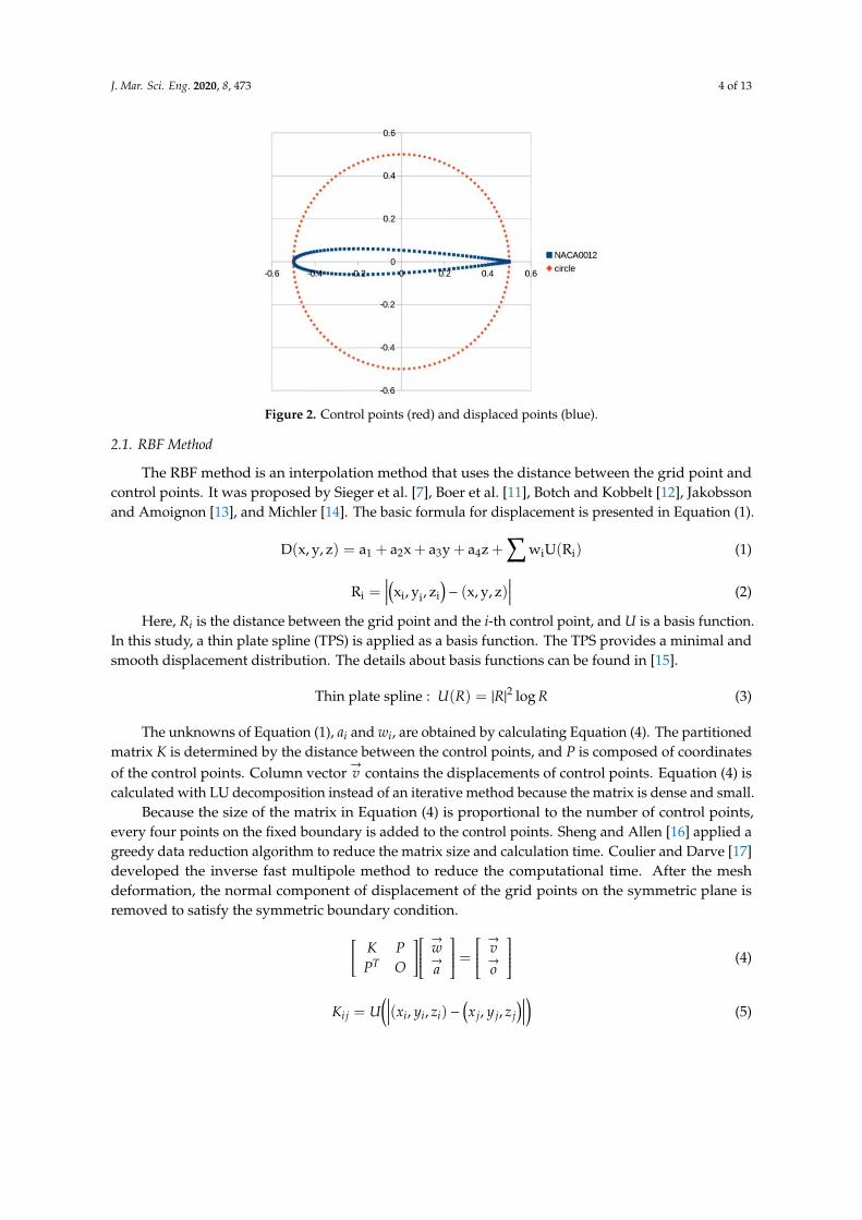
In this section, the RBF and IDW methods are introduced and compared. In addition, an improved RBF method to remedy its shortcomings is proposed. A mesh for a circular cylinder was deformed to the mesh of NACA 0012 using the RBF, IDW, and proposed methods. The red points in Figure 2 denote the control points on the surface of the circle and the blue ones indicate the displaced points on the surface of NACA 0012. The number of control points is 256 and the points move only in the vertical direction. The vertical movements make the normal vectors of the boundary faces rotate.

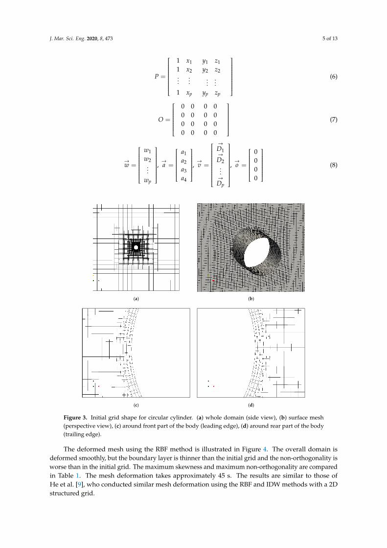
The initial grid for the circular cylinder is shown in Figure 3. The grid is a polyhedral mesh generated using snappyHexMesh, a standard built-in utility of OpenFOAM (The OpenFOAM Foundation Ltd., London, U.K.). The number of cells is 103,160 and the thickness of first boundary layer cell is 1% of the cylinder diameter. The top, bottom, right, and left boundaries were set as fixed boundary conditions. The front and back boundaries were set as symmetric boundary conditions. To satisfy the fixed boundary condition, the grid points of the fixed boundary were added to the control points. The displacements of the fixed boundary were set as zero.

Figure 1. Procedure of computational fluid dynamics (CFD)-based optimization. (a) Re-meshingmethod. (b) Mesh deforming method.

2. Mesh Deformation Methods

In this section, the RBF and IDW methods are introduced and compared. In addition, an improvedRBF method to remedy its shortcomings is proposed. A mesh for a circular cylinder was deformedto the mesh of NACA 0012 using the RBF, IDW, and proposed methods. The red points in Figure 2denote the control points on the surface of the circle and the blue ones indicate the displaced pointson the surface of NACA 0012. The number of control points is 256 and the points move only in thevertical direction. The vertical movements make the normal vectors of the boundary faces rotate.

The initial grid for the circular cylinder is shown in Figure 3. The grid is a polyhedral meshgenerated using snappyHexMesh, a standard built-in utility of OpenFOAM (The OpenFOAMFoundation Ltd., London, U.K.). The number of cells is 103,160 and the thickness of first boundarylayer cell is 1% of the cylinder diameter. The top, bottom, right, and left boundaries were set as fixedboundary conditions. The front and back boundaries were set as symmetric boundary conditions.To satisfy the fixed boundary condition, the grid points of the fixed boundary were added to the controlpoints. The displacements of the fixed boundary were set as zero.

J. Mar. Sci. Eng. 2020, 8, 473 4 of 13J. Mar. Sci. Eng. 2020, 8, 473 4 of 14

Figure 2. Control points (red) and displaced points (blue).

(a) (b)

(c) (d)

Figure 3. Initial grid shape for circular cylinder. (a) whole domain (side view), (b) surface mesh (perspective view), (c) around front part of the body (leading edge), (d) around rear part of the body (trailing edge).

Figure 2. Control points (red) and displaced points (blue).

2.1. RBF Method

The RBF method is an interpolation method that uses the distance between the grid point andcontrol points. It was proposed by Sieger et al. [7], Boer et al. [11], Botch and Kobbelt [12], Jakobssonand Amoignon [13], and Michler [14]. The basic formula for displacement is presented in Equation (1).

D(x, y, z) = a1 + a2x + a3y + a4z +∑

wiU(Ri) (1)

Ri =∣∣∣∣(xi, yi, zi

)− (x, y, z)

∣∣∣∣ (2)

Here, Ri is the distance between the grid point and the i-th control point, and U is a basis function.In this study, a thin plate spline (TPS) is applied as a basis function. The TPS provides a minimal andsmooth displacement distribution. The details about basis functions can be found in [15].

Thin plate spline : U(R) = |R|2 log R (3)

The unknowns of Equation (1), ai and wi, are obtained by calculating Equation (4). The partitionedmatrix K is determined by the distance between the control points, and P is composed of coordinatesof the control points. Column vector

→v contains the displacements of control points. Equation (4) is

calculated with LU decomposition instead of an iterative method because the matrix is dense and small.Because the size of the matrix in Equation (4) is proportional to the number of control points,

every four points on the fixed boundary is added to the control points. Sheng and Allen [16] applied agreedy data reduction algorithm to reduce the matrix size and calculation time. Coulier and Darve [17]developed the inverse fast multipole method to reduce the computational time. After the meshdeformation, the normal component of displacement of the grid points on the symmetric plane isremoved to satisfy the symmetric boundary condition.[

K PPT O

] →w→a = →v→o

(4)

Ki j = U(∣∣∣∣(xi, yi, zi) −

(x j, y j, z j

)∣∣∣∣) (5)

J. Mar. Sci. Eng. 2020, 8, 473 5 of 13

P =

1 x1 y1 z1

1 x2 y2 z2...

... ......

1 xp yp zp

(6)

O =

0 0 0 00 0 0 00 0 0 00 0 0 0

(7)

→w =

w1

w2...

wp

,→a =

a1

a2

a3

a4

,→v =

→

D1→

D2...→

Dp

,→o =

0000

(8)

J. Mar. Sci. Eng. 2020, 8, 473 4 of 14

Figure 2. Control points (red) and displaced points (blue).

(a) (b)

(c) (d)

Figure 3. Initial grid shape for circular cylinder. (a) whole domain (side view), (b) surface mesh (perspective view), (c) around front part of the body (leading edge), (d) around rear part of the body (trailing edge).

Figure 3. Initial grid shape for circular cylinder. (a) whole domain (side view), (b) surface mesh(perspective view), (c) around front part of the body (leading edge), (d) around rear part of the body(trailing edge).

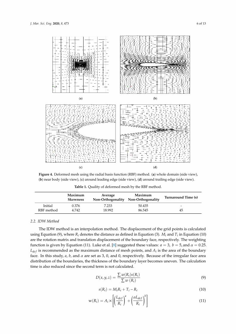
The deformed mesh using the RBF method is illustrated in Figure 4. The overall domain isdeformed smoothly, but the boundary layer is thinner than the initial grid and the non-orthogonality isworse than in the initial grid. The maximum skewness and maximum non-orthogonality are comparedin Table 1. The mesh deformation takes approximately 45 s. The results are similar to those ofHe et al. [9], who conducted similar mesh deformation using the RBF and IDW methods with a 2Dstructured grid.

J. Mar. Sci. Eng. 2020, 8, 473 6 of 13J. Mar. Sci. Eng. 2020, 8, 473 6 of 14

(a) (b)

(c) (d)

Figure 4. Deformed mesh using the radial basis function (RBF) method. (a) whole domain (side view), (b) near body (side view), (c) around leading edge (side view), (d) around trailing edge (side view).

Table 1. Quality of deformed mesh by the RBF method.

Maximum Skewness

Average Non-Orthogonality

Maximum Non-Orthogonality

Turnaround Time (s)

Initial 0.376 7.233 50.435 - RBF

method 4.742 18.992 86.545 45

2.2. IDW Method

The IDW method is an interpolation method. The displacement of the grid points is calculated using Equation (9), where 푅 denotes the distance as defined in Equation (3). 푀 and 푇 in Equation (10) are the rotation matrix and translation displacement of the boundary face, respectively. The weighting function is given by Equation (11). Luke et al. [8] suggested these values: 푎 = 3, 푏 =5, and 훼 = 0.25. 퐿 is recommended as the maximum distance of mesh points, and 퐴 is the area of the boundary face. In this study, 푎, 푏, and 훼 are set as 3, 0, and 0, respectively. Because of the irregular face area distribution of the boundaries, the thickness of the boundary layer becomes uneven. The calculation time is also reduced since the second term is not calculated.

Figure 4. Deformed mesh using the radial basis function (RBF) method. (a) whole domain (side view),(b) near body (side view), (c) around leading edge (side view), (d) around trailing edge (side view).

Table 1. Quality of deformed mesh by the RBF method.

MaximumSkewness

AverageNon-Orthogonality

MaximumNon-Orthogonality Turnaround Time (s)

Initial 0.376 7.233 50.435 -RBF method 4.742 18.992 86.545 45

2.2. IDW Method

The IDW method is an interpolation method. The displacement of the grid points is calculatedusing Equation (9), where Ri denotes the distance as defined in Equation (3). Mi and Ti in Equation (10)are the rotation matrix and translation displacement of the boundary face, respectively. The weightingfunction is given by Equation (11). Luke et al. [8] suggested these values: a = 3, b = 5, and α = 0.25.Lde f is recommended as the maximum distance of mesh points, and Ai is the area of the boundaryface. In this study, a, b, and α are set as 3, 0, and 0, respectively. Because of the irregular face areadistribution of the boundaries, the thickness of the boundary layer becomes uneven. The calculationtime is also reduced since the second term is not calculated.

D(x, y, z) =∑

w(Ri)s(Ri)∑w (Ri)

(9)

s(Ri) = MiRi + Ti −Ri (10)

w(Ri) = Ai ×

(Lde f

Ri

)a

+

(αLde f

Ri

)b (11)

J. Mar. Sci. Eng. 2020, 8, 473 7 of 13

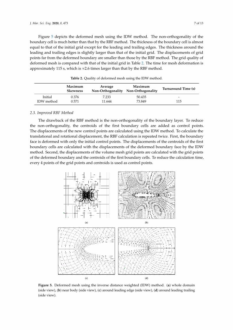
Figure 5 depicts the deformed mesh using the IDW method. The non-orthogonality of theboundary cell is much better than that by the RBF method. The thickness of the boundary cell is almostequal to that of the initial grid except for the leading and trailing edges. The thickness around theleading and trailing edges is slightly larger than that of the initial grid. The displacements of gridpoints far from the deformed boundary are smaller than those by the RBF method. The grid quality ofdeformed mesh is compared with that of the initial grid in Table 2. The time for mesh deformation isapproximately 115 s, which is ≈2.6 times larger than that by the RBF method.

Table 2. Quality of deformed mesh using the IDW method.

MaximumSkewness

AverageNon-Orthogonality

MaximumNon-Orthogonality Turnaround Time (s)

Initial 0.376 7.233 50.435 -IDW method 0.571 11.644 73.849 115

2.3. Improved RBF Method

The drawback of the RBF method is the non-orthogonality of the boundary layer. To reducethe non-orthogonality, the centroids of the first boundary cells are added as control points.The displacements of the new control points are calculated using the IDW method. To calculate thetranslational and rotational displacement, the RBF calculation is repeated twice. First, the boundaryface is deformed with only the initial control points. The displacements of the centroids of the firstboundary cells are calculated with the displacements of the deformed boundary face by the IDWmethod. Second, the displacements of the volume mesh grid points are calculated with the grid pointsof the deformed boundary and the centroids of the first boundary cells. To reduce the calculation time,every 4 points of the grid points and centroids is used as control points.

J. Mar. Sci. Eng. 2020, 8, 473 7 of 14

퐷(푥, 푦, 푧) =∑ 푤(푅 )푠(푅 )

∑ 푤 (푅 ) (9)

푠(푅 ) = 푀 푅 + 푇 − 푅 (10)

w(푅 ) = 퐴 ×퐿

푅+

훼퐿푅

(11)

Figure 5 depicts the deformed mesh using the IDW method. The non-orthogonality of the boundary cell is much better than that by the RBF method. The thickness of the boundary cell is almost equal to that of the initial grid except for the leading and trailing edges. The thickness around the leading and trailing edges is slightly larger than that of the initial grid. The displacements of grid points far from the deformed boundary are smaller than those by the RBF method. The grid quality of deformed mesh is compared with that of the initial grid in Table 2. The time for mesh deformation is approximately 115 s, which is ≈2.6 times larger than that by the RBF method.

(a) (b)

(c) (d)

Figure 5. Deformed mesh using the inverse distance weighted (IDW) method. (a) whole domain (side view), (b) near body (side view), (c) around leading edge (side view), (d) around leading trailing (side view).

Figure 5. Deformed mesh using the inverse distance weighted (IDW) method. (a) whole domain(side view), (b) near body (side view), (c) around leading edge (side view), (d) around leading trailing(side view).

J. Mar. Sci. Eng. 2020, 8, 473 8 of 13

It is difficult to apply both the RBF and IDW methods to problems involving the free surfacebecause the grid around the free surface has to be aligned to the free surface to minimize the numericaldiffusion of the volume of fluid function (VOF). Therefore, the deformable region must be limited.The cells around the deformed boundary are designated as deformable cells, while those outside of theregions are set as frozen cells. The faces sheared by the deformable and frozen cells are designated asfixed faces. The points on the fixed faces are added to the fixed control points.

Figure 6 displays the deformed mesh. The non-orthogonality of the boundary cell is better thanthose by the RBF and IDW methods. The thickness of the boundary cells around the leading andtrailing edges is well preserved. The cells in yellow circle are deformable cells.

J. Mar. Sci. Eng. 2020, 8, 473 8 of 14

Table 2. Quality of deformed mesh using the IDW method.

Maximum Skewness

Average Non-Orthogonality

Maximum Non-Orthogonality

Turnaround Time (s)

Initial 0.376 7.233 50.435 - IDW

method 0.571 11.644 73.849 115

2.3. Improved RBF Method

The drawback of the RBF method is the non-orthogonality of the boundary layer. To reduce the non-orthogonality, the centroids of the first boundary cells are added as control points. The displacements of the new control points are calculated using the IDW method. To calculate the translational and rotational displacement, the RBF calculation is repeated twice. First, the boundary face is deformed with only the initial control points. The displacements of the centroids of the first boundary cells are calculated with the displacements of the deformed boundary face by the IDW method. Second, the displacements of the volume mesh grid points are calculated with the grid points of the deformed boundary and the centroids of the first boundary cells. To reduce the calculation time, every 4 points of the grid points and centroids is used as control points.

It is difficult to apply both the RBF and IDW methods to problems involving the free surface because the grid around the free surface has to be aligned to the free surface to minimize the numerical diffusion of the volume of fluid function (VOF). Therefore, the deformable region must be limited. The cells around the deformed boundary are designated as deformable cells, while those outside of the regions are set as frozen cells. The faces sheared by the deformable and frozen cells are designated as fixed faces. The points on the fixed faces are added to the fixed control points.

Figure 6 displays the deformed mesh. The non-orthogonality of the boundary cell is better than those by the RBF and IDW methods. The thickness of the boundary cells around the leading and trailing edges is well preserved. The cells in yellow circle are deformable cells.

(a) (b)

J. Mar. Sci. Eng. 2020, 8, 473 9 of 14

(c) (d)

Figure 6. Deformed mesh using the RBF method with additional control points. (a) whole domain (side view), (b) near body (side view), (c) around leading edge (side view), (d) around trailing edge (side view).

The quality of the deformed mesh is compared with the initial mesh in Table 3. The deformed mesh quality using the proposed method is as good as that by the IDW method. Moreover, the proposed method is much faster than the others owing to the limited deformation region.

Table 3. Quality of the deformed mesh using the proposed method.

Maximum Skewness

Average Non-Orthogonality

Maximum Non-Orthogonality

Turnaround Time (s)

Initial 0.376 7.233 50.435 - Proposed method

0.782 12.141 74.920 13

3. Mesh Deformation for Hull Form Variation

The proposed mesh deformation method was applied to the mesh for ship resistance calculation to examine its applicability to CFD-based optimization. The ship used in the calculations is the JBC model. The scale ratio and the draft are 1:40 and 0.4125 m (16.5 m in full scale), respectively. The speed is 1.179 m/s (14.5 knots in the model).

The initial grid used for the JBC resistance calculation is illustrated in Figure 7. The number of cells is 2,402,361. The Y+ of first layer thickness is approximately 50 and the number of boundary layers is 4. The expansion ratio of the boundary layer is approximately 1.3. The running attitude of the ship is fixed as even keel condition. The simulation was conducted using interFoam, a standard solver of OpenFOAM. kOmegaSST and nutUSpaldingWallFunction were used as the turbulence model and wall function, respectively.

Figure 6. Deformed mesh using the RBF method with additional control points. (a) whole domain(side view), (b) near body (side view), (c) around leading edge (side view), (d) around trailing edge(side view).

The quality of the deformed mesh is compared with the initial mesh in Table 3. The deformedmesh quality using the proposed method is as good as that by the IDW method. Moreover, theproposed method is much faster than the others owing to the limited deformation region.

J. Mar. Sci. Eng. 2020, 8, 473 9 of 13

Table 3. Quality of the deformed mesh using the proposed method.

MaximumSkewness

AverageNon-Orthogonality

MaximumNon-Orthogonality Turnaround Time (s)

Initial 0.376 7.233 50.435 -Proposed method 0.782 12.141 74.920 13

3. Mesh Deformation for Hull Form Variation

The proposed mesh deformation method was applied to the mesh for ship resistance calculationto examine its applicability to CFD-based optimization. The ship used in the calculations is the JBCmodel. The scale ratio and the draft are 1:40 and 0.4125 m (16.5 m in full scale), respectively. The speedis 1.179 m/s (14.5 knots in the model).

The initial grid used for the JBC resistance calculation is illustrated in Figure 7. The number ofcells is 2,402,361. The Y+ of first layer thickness is approximately 50 and the number of boundarylayers is 4. The expansion ratio of the boundary layer is approximately 1.3. The running attitude of theship is fixed as even keel condition. The simulation was conducted using interFoam, a standard solverof OpenFOAM. kOmegaSST and nutUSpaldingWallFunction were used as the turbulence model andwall function, respectively.J. Mar. Sci. Eng. 2020, 8, 473 10 of 14

(a)

(b)

Figure 7. Grid shape for Japan bulk carrier (JBC) resistance calculation. (a) whole domain (side view), (b) surface mesh of fore body (side view).

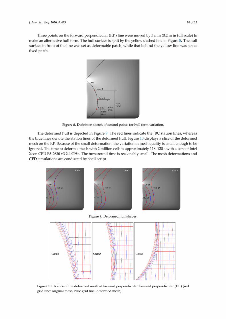
Three points on the forward perpendicular (F.P.) line were moved by 5 mm (0.2 m in full scale) to make an alternative hull form. The hull surface is split by the yellow dashed line in Figure 8. The hull surface in front of the line was set as deformable patch, while that behind the yellow line was set as fixed patch.

Figure 8. Definition sketch of control points for hull form variation.

Figure 7. Grid shape for Japan bulk carrier (JBC) resistance calculation. (a) whole domain (side view),(b) surface mesh of fore body (side view).

J. Mar. Sci. Eng. 2020, 8, 473 10 of 13

Three points on the forward perpendicular (F.P.) line were moved by 5 mm (0.2 m in full scale) tomake an alternative hull form. The hull surface is split by the yellow dashed line in Figure 8. The hullsurface in front of the line was set as deformable patch, while that behind the yellow line was set asfixed patch.

J. Mar. Sci. Eng. 2020, 8, 473 10 of 14

(a)

(b)

Figure 7. Grid shape for Japan bulk carrier (JBC) resistance calculation. (a) whole domain (side view), (b) surface mesh of fore body (side view).

Three points on the forward perpendicular (F.P.) line were moved by 5 mm (0.2 m in full scale) to make an alternative hull form. The hull surface is split by the yellow dashed line in Figure 8. The hull surface in front of the line was set as deformable patch, while that behind the yellow line was set as fixed patch.

Figure 8. Definition sketch of control points for hull form variation. Figure 8. Definition sketch of control points for hull form variation.

The deformed hull is depicted in Figure 9. The red lines indicate the JBC station lines, whereasthe blue lines denote the station lines of the deformed hull. Figure 10 displays a slice of the deformedmesh on the F.P. Because of the small deformation, the variation in mesh quality is small enough to beignored. The time to deform a mesh with 2 million cells is approximately 118–120 s with a core of IntelXeon CPU E5-2630 v3 2.4 GHz. The turnaround time is reasonably small. The mesh deformations andCFD simulations are conducted by shell script.

J. Mar. Sci. Eng. 2020, 8, 473 11 of 14

The deformed hull is depicted in Figure 9. The red lines indicate the JBC station lines, whereas the blue lines denote the station lines of the deformed hull. Figure 10 displays a slice of the deformed mesh on the F.P. Because of the small deformation, the variation in mesh quality is small enough to be ignored. The time to deform a mesh with 2 million cells is approximately 118–120 s with a core of Intel Xeon CPU E5-2630 v3 2.4 GHz. The turnaround time is reasonably small. The mesh deformations and CFD simulations are conducted by shell script.

Figure 9. Deformed hull shapes.

Figure 10. A slice of the deformed mesh at forward perpendicular forward perpendicular (F.P.) (red grid line: original mesh, blue grid line: deformed mesh).

The resistance histories of the JBC and deformed hulls are compared in Figure 11. The calculations of deformed hulls converged much faster than the JBC calculation because the result of the JBC calculation was used as the initial condition for the deformed hull resistance calculations. The calculation of the JBC resistance took approximately 60 s, whereas the calculation of deformed hulls took 20 s in flow time. The variations in the resistances are small because the hull form variation is small. The resistance coefficients are compared in Table 4.

Figure 9. Deformed hull shapes.

J. Mar. Sci. Eng. 2020, 8, 473 11 of 14

The deformed hull is depicted in Figure 9. The red lines indicate the JBC station lines, whereas the blue lines denote the station lines of the deformed hull. Figure 10 displays a slice of the deformed mesh on the F.P. Because of the small deformation, the variation in mesh quality is small enough to be ignored. The time to deform a mesh with 2 million cells is approximately 118–120 s with a core of Intel Xeon CPU E5-2630 v3 2.4 GHz. The turnaround time is reasonably small. The mesh deformations and CFD simulations are conducted by shell script.

Figure 9. Deformed hull shapes.

Figure 10. A slice of the deformed mesh at forward perpendicular forward perpendicular (F.P.) (red grid line: original mesh, blue grid line: deformed mesh).

The resistance histories of the JBC and deformed hulls are compared in Figure 11. The calculations of deformed hulls converged much faster than the JBC calculation because the result of the JBC calculation was used as the initial condition for the deformed hull resistance calculations. The calculation of the JBC resistance took approximately 60 s, whereas the calculation of deformed hulls took 20 s in flow time. The variations in the resistances are small because the hull form variation is small. The resistance coefficients are compared in Table 4.

Figure 10. A slice of the deformed mesh at forward perpendicular forward perpendicular (F.P.) (redgrid line: original mesh, blue grid line: deformed mesh).

J. Mar. Sci. Eng. 2020, 8, 473 11 of 13

The resistance histories of the JBC and deformed hulls are compared in Figure 11. The calculations ofdeformed hulls converged much faster than the JBC calculation because the result of the JBC calculationwas used as the initial condition for the deformed hull resistance calculations. The calculation of theJBC resistance took approximately 60 s, whereas the calculation of deformed hulls took 20 s in flowtime. The variations in the resistances are small because the hull form variation is small. The resistancecoefficients are compared in Table 4.

J. Mar. Sci. Eng. 2020, 8, 473 12 of 14

(a)

(b)

Figure 11. Comparisons of resistance convergence histories. (a) whole time, (b) zoomed.

Table 4. Comparison of resistances of the JBC and deformed hull.

JBC Case 1 Case 2 Case 3 Resistance coefficient 4.186×10-3 4.187×10-3 4.184×10-3 4.186×10-3

The pressure distributions and wave height contours are compared in Figures 12 and 13, respectively. It was found that the result of the initial hull form can be used as the initial condition for the deformed hull resistance calculation.

Figure 12. Comparison of pressure distributions around the bow (left: JBC only, right: JBC and deformed hull).

Figure 11. Comparisons of resistance convergence histories. (a) whole time, (b) zoomed.

Table 4. Comparison of resistances of the JBC and deformed hull.

JBC Case 1 Case 2 Case 3

Resistancecoefficient 4.186 × 10−3 4.187 × 10−3 4.184 × 10−3 4.186 × 10−3

The pressure distributions and wave height contours are compared in Figures 12 and 13,respectively. It was found that the result of the initial hull form can be used as the initial condition forthe deformed hull resistance calculation.

J. Mar. Sci. Eng. 2020, 8, 473 12 of 13

J. Mar. Sci. Eng. 2020, 8, 473 12 of 14

(a)

(b)

Figure 11. Comparisons of resistance convergence histories. (a) whole time, (b) zoomed.

Table 4. Comparison of resistances of the JBC and deformed hull.

JBC Case 1 Case 2 Case 3 Resistance coefficient 4.186×10-3 4.187×10-3 4.184×10-3 4.186×10-3

The pressure distributions and wave height contours are compared in Figures 12 and 13, respectively. It was found that the result of the initial hull form can be used as the initial condition for the deformed hull resistance calculation.

Figure 12. Comparison of pressure distributions around the bow (left: JBC only, right: JBC and deformed hull).

Figure 12. Comparison of pressure distributions around the bow (left: JBC only, right: JBC anddeformed hull).J. Mar. Sci. Eng. 2020, 8, 473 13 of 14

Figure 13. Comparison of wave height contour around the bow.

4. Conclusions

In this study, two methods for mesh deformation, namely, the RBF and IDW methods, were compared. Moreover, an improved RBF method was proposed for a largely deformed mesh. The RBF method was much faster than the IDW method, but the quality of the deformed mesh using the IDW method was better than that by the RBF method. The quality of the deformed mesh by the RBF method was improved by adding the centroids of boundary cells to the control points. The displacements of the centroids were calculated using the IDW method. The deformable region was limited for the problem involving the free surface. The limitation also reduced the calculation time.

The improved RBF method was applied to the mesh for the JBC resistance calculation to validate its applicability. The resistance was calculated by varying the bow shape with three control points. It took approximately 120 s for the mesh to deform, which is short enough to apply to practical problems. The calculation result of the initial hull form was used as the initial condition for the deformed hull form, which reduced the calculation time to approximately one-third of that of the initial hull form. Thus, the improved RBF method proposed in this study is effective and efficient for hull form variation.

In the future, the CFD-based hull form optimization will be conducted using the proposed mesh deformation method together with an optimization algorithm such as sequential quadratic programming or an adjoint variable method.

Author Contributions: Conceptualization, K.-L.J. and S.-M.J.; methodology, K.-L.J.; validation K.-L.J.; formal analysis, K.-L.J.; investigation, K.-L.J. and S.-M.J.; resources, K.-L.J. and S.-M.J.; writing—original draft preparation, K.-L.J. and S.-M.J.; writing—review and editing, S.-M.J.; visualization, K.-L.J.; supervision, K.-L.J. and S.-M.J.; and funding acquisition, S.-M.J. All authors have read and agreed to the published version of the manuscript.

Funding: This study was supported by a research fund from Chosun University (K207177004).

Conflicts of Interest: The authors declare no conflicts of interest.

References

1. Kim, H.; Yang, C.; Noblesse, F. Hull form optimization for reduced resistance and improved seakeeping via practical designed-oriented CFD tools. In Proceedings of the 2010 Conference on Grand Challenges in Modeling and Simulation, Ottawa, ON, Canada, 11–14 July 2010.

2. Kim, H.; Yang, C. A new surface modification approach for CFD-based hull form optimization. J. Hydrodyn. 2010, 22, 503–508.

Figure 13. Comparison of wave height contour around the bow.

4. Conclusions

In this study, two methods for mesh deformation, namely, the RBF and IDW methods, werecompared. Moreover, an improved RBF method was proposed for a largely deformed mesh. The RBFmethod was much faster than the IDW method, but the quality of the deformed mesh using the IDWmethod was better than that by the RBF method. The quality of the deformed mesh by the RBF methodwas improved by adding the centroids of boundary cells to the control points. The displacementsof the centroids were calculated using the IDW method. The deformable region was limited for theproblem involving the free surface. The limitation also reduced the calculation time.

The improved RBF method was applied to the mesh for the JBC resistance calculation to validate itsapplicability. The resistance was calculated by varying the bow shape with three control points. It tookapproximately 120 s for the mesh to deform, which is short enough to apply to practical problems.The calculation result of the initial hull form was used as the initial condition for the deformed hullform, which reduced the calculation time to approximately one-third of that of the initial hull form.Thus, the improved RBF method proposed in this study is effective and efficient for hull form variation.

In the future, the CFD-based hull form optimization will be conducted using the proposedmesh deformation method together with an optimization algorithm such as sequential quadraticprogramming or an adjoint variable method.

Author Contributions: Conceptualization, K.-L.J. and S.-M.J.; methodology, K.-L.J.; validation K.-L.J.; formalanalysis, K.-L.J.; investigation, K.-L.J. and S.-M.J.; resources, K.-L.J. and S.-M.J.; writing—original draft preparation,K.-L.J. and S.-M.J.; writing—review and editing, S.-M.J.; visualization, K.-L.J.; supervision, K.-L.J. and S.-M.J.; andfunding acquisition, S.-M.J. All authors have read and agreed to the published version of the manuscript.

Funding: This study was supported by a research fund from Chosun University (K207177004).

J. Mar. Sci. Eng. 2020, 8, 473 13 of 13

Conflicts of Interest: The authors declare no conflicts of interest.

References

1. Kim, H.; Yang, C.; Noblesse, F. Hull form optimization for reduced resistance and improved seakeepingvia practical designed-oriented CFD tools. In Proceedings of the 2010 Conference on Grand Challenges inModeling and Simulation, Ottawa, ON, Canada, 11–14 July 2010.

2. Kim, H.; Yang, C. A new surface modification approach for CFD-based hull form optimization. J. Hydrodyn.2010, 22, 503–508. [CrossRef]

3. Mahmood, S.; Huang, D. Computational fluid dynamics based bulbous bow optimization using a geneticalgorithm. J. Martine Sci. Appl. 2012, 11, 286–294. [CrossRef]

4. Zhang, S.; Zhang, B.; Tezdogan, T.; Xu, L.; Lai, Y. Computational fluid dynamics-based hull form optimizationusing approximation method. Eng. Appl. Comput. Fluid Mech. 2018, 12, 74–88. [CrossRef]

5. Sun, Z.X.; Song, J.J.; An, Y.R. Optimization of the head shape of the CRH3 high speed train. Sci. ChinaTechnol. Sci. 2010, 53, 3356–3364. [CrossRef]

6. Morris, A.M.; Allen, C.B.; Rendall, T.C.S. CFD-based optimization of aerofoils using radial basis functionsfor domain element parameterization and mesh deformation. Int. J. Numer. Meth. Fluids 2008, 58, 827–860.[CrossRef]

7. Sieger, D.; Menzel, S.; Botsch, M. On Shape Deformation Techniques for Simulation–Based Design Optimization,In New Challenge in Grid Generation and Adaptively for Scientific Computing; Springer Series: Cham, Switzerland,2015; pp. 281–303.

8. Luke, E.; Collins, E.; Blades, E. A fast mesh deformation method using explicit interpolation. J. Comput. Phys.2012, 231, 586–601. [CrossRef]

9. He, X.; Li, J.; Mader, C.A.; Yildirim, A.; Martins, J.R.R.A. Robust aerodynamic shape optimization-form acircle to an airfoil. Aerosp. Sci. Technol. 2019, 87, 48–61. [CrossRef]

10. Ding, L.; Lu, Z.; Guo, T. An efficient dynamic mesh generation method for complex multi-block structuredgrid. Adv. Appl. Math. Mech. 2014, 6, 120–134. [CrossRef]

11. Boer, A.; Van der Schoot, M.; Bijl, H. Mesh deformation based on radial basis function interpolation.Comput. Struct. 2007, 85, 784–795. [CrossRef]

12. Botch, M.; Kobbelt, L. Real-time shape editing using radial basis function. Comput. Graph. Forum 2005, 24,611–621. [CrossRef]

13. Jakobsson, S.; Amoignon, O. Mesh deformation using radial basis functions for gradient-based aerodynamicshape optimization. Comput. Fluids 2007, 36, 1119–1136. [CrossRef]

14. Michler, A.K. Aircraft control surface deflection using RBF-based mesh deformation. Int. J. Numer. Meth. Eng.2011, 88, 986–1007. [CrossRef]

15. Buhmann, M.D. Radial Basis Functions: Theory and Implementations; Cambridge University Press: Cambridge,UK, 2003; ISBN 978-0511040207.

16. Sheng, C.; Allen, C.B. Efficient mesh deformation using radial basis functions on unstructured meshes.AIAA J. 2013, 51, 707–720. [CrossRef]

17. Coulier, P.; Darve, E. Efficient mesh deformation based on radial basis function interpolation by means of theinverse fast multipole method. Comput. Methods Appl. Mech. Eng. 2016, 308, 286–309. [CrossRef]

© 2020 by the authors. Licensee MDPI, Basel, Switzerland. This article is an open accessarticle distributed under the terms and conditions of the Creative Commons Attribution(CC BY) license (http://creativecommons.org/licenses/by/4.0/).