Paper prepared for the conference on “Divorce in Cross-National Perspective: A European Research Network” European University Institute, Florence, Italy November 14 & 15, 2002 DRAFT A Meta-Analysis of German Research on Divorce Risks Michael Wagner and Bernd Weiß Research Institute for Sociology University of Cologne Greinstr. 2 50939 Cologne [email protected][email protected]
Transcript
Paper prepared for the conference on “Divorce in Cross-National Perspective: A European Research Network”
European University Institute, Florence, ItalyNovember 14 & 15, 2002
DRAFT
A Meta-Analysis of German Research on Divorce Risks
Michael Wagner
and
Bernd Weiß
Research Institute for SociologyUniversity of Cologne
The aim of the paper is to evaluate divorce studies in Germany and to apply meta-analytic techniques in order to summarize the results of this research. Literatureresearch identified 42 studies published between 1987 and 2001. These studies uselongitudinal data from seven projects and all studies estimate event history modelswith the divorce rate as dependent variable. In sum, they examine 399 different riskfactors and report 3730 effects. Results of the meta-analysis are threefold. First, thereare methodological problems in the field of meta-analysis that are not resolved in avery satisfactory way. Second, no theory of divorce has been tested in detail, rathersingle hypotheses have been examined which were derived from exchange ormicroeconomic theory. Third, divorce research can be improved by a more cumulativedesign which means that we need more studies conducting a replication of existingempirical findings.
1This research was supported by the German Science Foundation from July2000 to July 2001 (WA 1502/1-1). We thank Hans-Peter Blossfeld (Bamberg) forhelpful comments on an earlier version of the manuscript.
2
1 Problem1
During the past twenty years German sociology experienced a boom of divorcestudies. This development was mainly caused by methodological innovations thatenabled a reliable longitudinal assessment of marital histories, e.g. retrospectively inlife course research or prospectively in panel studies. The aim of this paper is toevaluate the studies on divorce risks in Germany. So many divorce risks have beenreported that it became unclear what we really know about the determinants of maritalinstability (Hartmann 1989; Dorbritz/Gärtner 1998). Which theories or hypotheseshave been confirmed by empirical findings? Is research undertaken cumulatively? Areempirical findings presented in such a way that their evaluation is possible?
The evaluation of empirical research is usually done by qualitative reviews. However,this kind of research synthesis shows various shortcomings. The two most seriousones result from non-systematical and incomplete literature research as well as froman inadequate integration and interpretation of diverging quantitative results(Wagner/Weiß 2001). In order to overcome these disadvantages, we apply meta-analytic methods. Besides primary and secondary research, this method stands for athird type of empirical social research. Meta-analysis is primarily concerned with thequantitative integration of published empirical findings (Glass 1976). However, itallows not only their integration but also the explanation of their heterogeneity.
Meta-analysis is rather unknown, especially in German sociology. Only Künzler (1994)and Engelhardt (2000) mention it, the latter as part of a survey of study designs indemography. Some others call their study a meta-analysis, as in fact they summarizecharacteristics of numerous publications, but without systematically investigatingquantitative results (Bretschneider 1997; Hartmann 1999). In other disciplines thansociology, like medical science, psychology and educational science, meta-analysishas gained much more popularity, in Germany as well as elsewhere. In psychology,the outcomes of a great number of studies that are interested in the success of certaintherapies have been summarized by meta-analyses. In medical science, the „EvidenceBased Medicine“ has already been institutionalized (Altman 2000; Petitti 2000; Suttonet al. 2000). Numerous handbooks and monographies on meta-analysis underline theimportance of this research area (Bortz/Olkin 1985; Hunter/Schmidt 1990;Lipsey/Wilson 2001; Rosenthal 1991; Schultz-Gambard 1987; Sutton et al. 2000).
3
2 Meta-analysis
To perform a meta-analysis does not differ much from other types of social research(Diekmann 1997; Schnell et al. 1995). We apply a five stage-model proposed byCooper (1982):
1. Problem/research question2. Literature research3. Data evaluation and coding4. Data analysis 5. Presentation of results
2.1 Literature ResearchThe population of our meta-analysis is defined as the totality of empirical studies fromGermany investigating marital stability and using the divorce rate as the dependentvariable. These studies use longitudinal data on marriages and partnerships. Before1990, only studies of West Germany, after 1990 studies of West and East Germanywere included.
A comprehensive literature research is necessary for any meta-analysis, including alltypes of publications and research reports. A detailed description of literature researchprocedures is given by Lipsey/Wilson (2001) and White (1994). In the present case,we started with a stock of 15 studies. Then a systematical search using several socialscience literature databases was undertaken (Family Studies Database, Popline,SSCI, SOLIS, FORIS, Sociological Abstracts, IHS, PsycINFO and PSYNDEX).References of publications were examined for further studies. The literature researchwas finished in spring 2001 (for details see Wagner/Weiß 2001; Weiß 2001).
Finally, 42 publications could be identified that matched the search criteria. They werepublished between 1987 and 2001. Half of all publications appeared before 1998.Many articles were published after 1997, because at this point of time the results ofthe Mannheim Research Project „Determinants of Divorces“ had been released.
In Germany, the relevant divorce studies use data samples from seven larger projectsof the Social Sciences. These are the Mannheim Research Project ‘Determinants ofDivorce’, the German Socio-Economic Panel, the Family Survey of the German YouthInstitute, the German Life History Study (Max Planck Institute for Human
2See the number of identification as it is found in the bibliography of the studiesthat have been included in the meta-analysis.
4
Development), the Family and Fertility Survey of Germany, the General Social Surveyof the Social Sciences and the Cologne Longitudinal Study of Gymnasium graduates.Most of the publications are taken from the Mannheim Research Project, followed bythe Family Survey (Table 1).
Table 1: Number of publications by year of publication and studyYear Study Total2
Determinants of Divorce` ; GSEP: German Socio-Economic Panel(DIW, Berlin); FS: Family Survey of the German Youth Institute (DJI, Munich); GLHS: German LifeHistory Study (MPI, Berlin); FFS: Family and Fertility Survey; GSS: General Social Survey of the SocialStudies; KLS: Cologne Longitudinal Study of Gymnasium Graduates.
2 Klein‘s (1999; No. 32 and 33) study has been counted twice, so the total number of publications hasbeen artificially increased by an additional publication.
Literature research revealed a number of anomalies. We ignored double publicationsof identical or nearly identical texts (cf. publication No. 232 and Diekmann/Klein 1993as well as publication No. 2 and Babka von Gostomski 1999). If a paper has beenpublished twice with substantial modifications this was counted as two publicationsand both went into the meta-analysis (cf. publications No. 7 and 34). Moreover, it ispossible that publications include empirical results which are based on two differentsamples. These publications have been registered as two independent cases (cf.publications No. 32 and 33).
5
Study
Publication A Publication B Publication C
Subgroup A Subgroup B
M odel A M odel B
Unit of analysis
Sampling unit
Divorce risk A
D ivo rce risk B
D ivo rce risk C
D ivorce risk D
E ffect size A
E ffect size B
E ffect size C
E ffect size D
E ffect size A
E ffect size B
E ffect size D
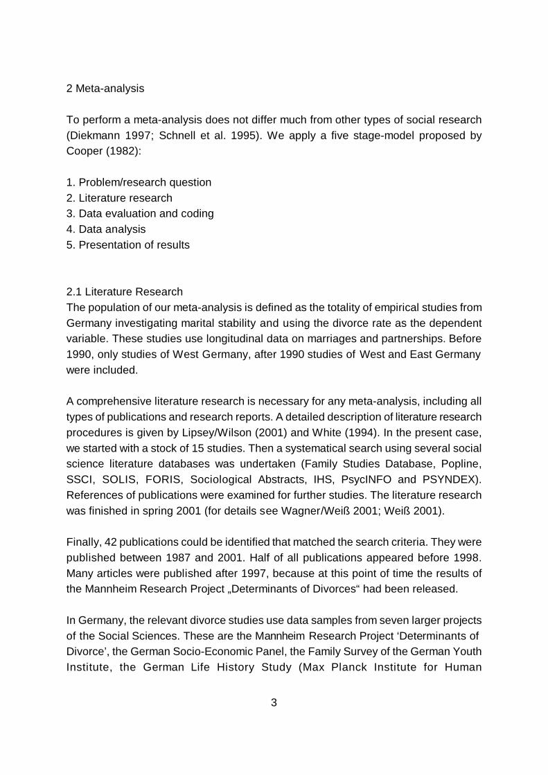
2.2 Levels of AnalysisWe distinguish between three basic concepts: study, publication and effect size.These concepts are ordered hierarchically (figure 1): ‘study’ is defined as the datasource or data sample, ‘publications’ report empirical results that are based onindividual studies, and an ‘effect size’ is a standardized research outcome which refersto statistics that capture the degree of association between variables (Hedges/Olkin1985). In our case, the only type of research outcomes are regression coefficients.
Figure 1: Levels of Meta-Analysis
In meta-analysis, single publications can be regarded as the sampling units andreported effect sizes can be regarded as the units of analysis. The state of researchcould be related to the study level.
It is important to note that empirical results might be valid only for specific subgroups.Sometimes, divorce risks are reported for West or for East Germany or for differentmarriage cohorts. Rather often for every single subgroup several event history modelsare estimated. Each of these models includes a different combination of covariates.
6
Consequently, the effect sizes do not only depend on the studies or on thecharacteristics of the underlying sample, but also on the particular subgroup and onthe particular specification of the model.
Altogether 3730 effects have been coded which have been reported for 399 variables -the determinantes of divorce. This huge number of variables results from the fact thatsome of them only differ with respect to value categorization or reference groups,although they measure the same theoretical concept. The variables and their effectshave been estimated in 515 models (Cox-model 71.3%; sickle model 11.8%;exponential model 9.7%; generalized log-logistic model 4.1%; remaining modelspecifications 3.1%). On an average, 7.2 covariate effects have been observed foreach model and 9.3 covariate effects were counted for each variable.
2.3 Collecting and Coding DataIt is not only justified to collect data on reported statistical results like singlecoefficients, levels of significance, or standard errors. As study characteristics mightaffect statistical results and therefore account for their heterogeneity, also studyvariables like type of institutional affiliation, type of financial support, or year of startand end of the project are of interest (Lipsey 1994; Lipsey/Wilson 2000).
In all publications divorce rates are analyzed by multivariate methods of event-analysis. However, each analysis is based on different variables. The theoretical andtechnical problem is to identify, to define and to sort this variety of variables and toassign effect sizes. It was necessary to develop a detailed schema which mergesvariables of the same meaning, operationalization and reference group. Based on 15divorce studies, a preleminary classification was developed. The categorizationschema broadly followed the ‘Thesaurus Social Sciences’ of the InformationszentrumSozialwissenschaften (1999) that uses eight categories: demography and other;marriage, family or kin and other networks; education; occupation; religion; nationality;spatial environment; property. Each of these categories was further divided intoseveral subgroups. Altogether, 399 codes had been assigned which means that weidentified 399 different determinants of divorce.
The hierarchical arrangement of data corresponds to a special type of data storageand data organization. Instead of storing data in an inappropriate rectangle matrix,which is done by MS-EXCEL or SPSS, we made use of a relational database. It allowsa more flexible use of data, and data retrieval account for different levels of analysis.A detailed description of data coding and data organization is given by Wagner/Weiß
7
(2001) and Weiß (2001). The statistical analyses have been realized by the software“R: A Language for Data Analysis and Graphics” (Ihaka/Gentleman 1996). Some ofthe already existing analysis functions could be taken over, in other cases theprogramming of new functions was necessary.
2.4 Data AnalysisData analysis is performed in four steps: preparation of data, integration of effectsizes, tests for homogeneity and detailed subgroup analysis. The outcome of effectsize integration is a set of different and pooled divorce factors. An analysis ofgraphical curves has not been realized (Weiß 2001). Integration will be done by usingtwo different methods: vote-counting and calculating mean effect sizes.
2.4.1 Vote-countingVote-counting is somewhere in between qualitative and quantitative review. It countssignificant positive, significant negative and non-significant effects. The modalcategory is regarded to be the best estimator concerning the direction of the effectbetween the independent and the dependent variable (Light/Smith 1971).
This method shows some serious statistical shortcomings (Fricke/Treinies 1985;Hedges/Olkin 1985; Wolf 1986). Additionally, Glass (1976) points out that vote-counting does not consider the magnitude of the correlation between two variables.
2.4.2 Estimation of mean effect sizesMany authors describe meta-analytical methods for pooling bivariate statistics (e.g.correlation coefficients, rank order correlations etc.) (Bortz/Döring 1995). Lessinformation exists on synthesizing regression coefficients from multivariate eventhistory models (cf. Greenland 1987). Many meta-analysts use such regressioncoefficients without giving any reasons (Karney/Bradbury 1995; Amato/Keith 1991;Amato 2001).
Another difficulty has to do with the aggregation of effect sizes that stem from modelsthat are differently specified. Coefficients from bivariate or multivariate methods differaccording to their magnitudes and standard errors. Following Lipsey/Wilson (2001),meta-analysis misses adequate procedures of multivariate result integration (e.g.factor analysis or multiple regression). Only very few authors discuss thismethodological problem (Amato 2001; Lipsey/Wilson 2001: 67 ff. and other meta-analyses cited in this book).
8
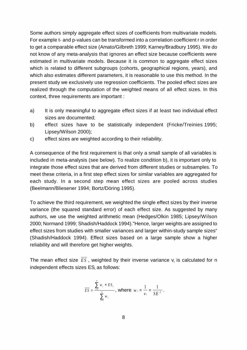
Some authors simply aggregate effect sizes of coefficients from multivariate models.For example t- and p-values can be transformed into a correlation coefficient r in orderto get a comparable effect size (Amato/Gilbreth 1999; Karney/Bradbury 1995). We donot know of any meta-analysis that ignores an effect size because coefficients wereestimated in multivariate models. Because it is common to aggregate effect sizeswhich is related to different subgroups (cohorts, geographical regions, years), andwhich also estimates different parameters, it is reasonable to use this method. In thepresent study we exclusively use regression coefficients. The pooled effect sizes arerealized through the computation of the weighted means of all effect sizes. In thiscontext, three requirements are important :
a) It is only meaningful to aggregate effect sizes if at least two individual effectsizes are documented;
b) effect sizes have to be statistically independent (Fricke/Treinies 1995;Lipsey/Wilson 2000);
c) effect sizes are weighted according to their reliability.
A consequence of the first requirement is that only a small sample of all variables isincluded in meta-analysis (see below). To realize condition b), it is important only tointegrate those effect sizes that are derived from different studies or subsamples. Tomeet these criteria, in a first step effect sizes for similar variables are aggregated foreach study. In a second step mean effect sizes are pooled across studies(Beelmann/Bliesener 1994; Bortz/Döring 1995).
To achieve the third requirement, we weighted the single effect sizes by their inversevariance (the squared standard error) of each effect size. As suggested by manyauthors, we use the weighted arithmetic mean (Hedges/Olkin 1985; Lipsey/Wilson2000; Normand 1999; Shadish/Haddock 1994).”Hence, larger weights are assigned toeffect sizes from studies with smaller variances and larger within-study sample sizes“(Shadish/Haddock 1994). Effect sizes based on a large sample show a higherreliability and will therefore get higher weights.
The mean effect size , weighted by their inverse variance vi is calculated for nE S
independent effects sizes ESi as follows:
, where .E S
w E S
w
i ii
n
ii
n=×
=
=
∑
∑1
1
wv S E
ii
= =1 1
2
9
The inverse variance vi is a weight assigned to the study and equals the inversesquared standard error (see appendix).
2.4.3 Effect size distributions Two distribution models of effect sizes have to be distinguished. The fixed effectsmodel assumes all effect sizes to come from one study population. It thus estimatesonly one population effect size and differences of effect sizes between studies areignored. The random effects model assumes the population parameters to berandomly distributed and located around a so-called “superpopulation”. The totalvariance of effect size estimates reflects both a study-within-variance and a study-between-variance (Shadish/Haddock 1994):
(see appendix) . v vi i* = +σθ
2
In the present case, the pooled effect sizes are expected to be heterogeneous,because the different effect sizes are based on different subgroups or modelspecifications (cf. above). Especially, the integration of partial coefficients is notsuccessfully solved. Coefficients from different models do not estimate the sameparameter. Therefore, we particularly make use of random effects models and expectresults of strong heterogeneity. We cannot address the question to what extentheterogeneity analyses could assess how the variety of model specifications affect themean effect size.
Homogeneity tests are applied to decide whether a distribution model with random orwith fixed effects is appropriate. In many cases these tests are based on the so-calledQ-statistic (cf. Hedges/Olkin 1985; Normand 1999; White 1999). We do not considerother homogeneity tests like for example the Likelihood Ratio Test (Hedges/Olkin1985). With k-1 degrees of freedom, the Q-statistic follows a Chi2 distribution with keffect sizes:
.Q w E S E Si i
i
k
= −=
∑ ( ) 2
1
If Q exceeds the critical value of the Chi2 distribution, the null hypothesis of ahomogeneous distribution has to be rejected. Hence, the distribution of effect sizeswould be assumed to be heterogeneous. It would be possible to conduct furtheranalyses that identify the determinants of heterogeneity. Those analyses are restricted
10
to large sample sizes and could therefore not be applied in the present study. Instead,we compute the weighting factor as the weighted average mean based on a randomeffects model.
2.4.4 Estimation of weightsSerious problems emerge if publications do not report sufficient information to conducta meta-analysis. This is especially true in case of missing standard errors of the effectsizes: only nine publications (21.4 percent of all publications) report standard errors ort-values. The remaining publications only offer information about significance levelsusing the well known ‘star symbolism’. To estimate the standard errors the giveninformation should be used at the best possible degree. Therefore, different estimationmethods can be found which basically refer to three different levels of information:
(1) At best, publications report exact information on standard errors, and the methodsdescribed in section 2.4.2. can be applied. Only effect sizes of the same type can beaggregated (
�- or � -coefficients). We decided to aggregate
�-coefficients. Hence, � -
coefficients had to be converted following �
=ln( � ) with SE=�
/t, where t= � /SE.
(2) The equation above can also be used if t-values are reported. There is nodifference between � - or
�-coefficients, because the computation of a t-value does not
depend on effect size types.
(3) As already stated, some publications only report intervals of significance levels,e.g. 0.01 < p < 0.05. In this case, the appropriate z-value can still be computed (thatis the upper bound of the interval) and we get SE=
�/Z.
We define effect sizes as non-significant if no significance levels are reported.Following Rosenthal (1991), we assign a p-value of 0.5 and the corresponding z-valueof 0.0 (one-tailed) as non-significant. In our case, a two-tailed question is given, sothat z is set to 0.67. The estimation of the standard error can only be done veryroughly. Another method is to set
�-coefficients to zero. It is not known which of the
two methods produces less errors.
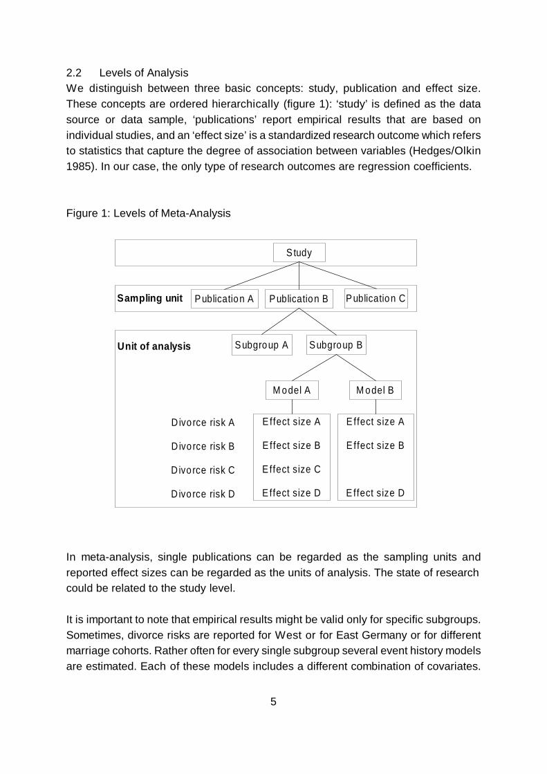
The whole decision process of finding an appropriate estimation procedure can bevisualized as a flowchart (figure 2). It also includes the so-called percent effects thatcan be computed from ( � -1) x 100.The figure shows the three already mentionedinformation levels which follow a hierarchical order. Within these three levels, it isimportant to distinguish between types of effect sizes in order to choose the
11
appropriate estimation method. To avoid confusion not all connections are shown(instead we use an encircled A).
12
S ta rt
S ta n d a rd e rr o r s (S E ) o r o th e ru se fu l s ta t is t ics fo r co m p u t in gwe ig h ts
In fo rm a tio n o ns ta n d a r d e rr o r s?
α-e ffe c t?
β-e ffe c t?
W h ich typ e o fe f fe c t?
% -e ffe c t?
S q u a re S E a n d we ig h t β' s
(1 ) t=α/S E(2 ) β= ln (α)(3 ) S E = β/t
(1 ) α=%/100+1(2 ) t=α /S E(3 ) β= ln (α)(4 ) S E = β/t
t -v a lu e s ?
α-e ffe c t?
β-e ffe c t?
% -e ffe c t?
(1 ) β= ln (α)(2 ) S E = β/t
(1 ) α=%/100+1(2) β= ln (α)(3 ) S E = β/t
S E = β/t
p - va lu e s?
α-e ffe c t?
β-e ffe c t?
% -e ffe c t?
(1 ) β= ln (α)(2 ) S E = β/z
(1 )α=%/100+1(2) β= ln (α)(3 ) S E =β/z
S E = β/z
W h ich typ e o fe f fe c t?
W h ich typ e o fe f fe c t?
A
A
A
A
A
Aye s
ye s
ye s
ye s
ye s
ye s
ye s
ye s
ye s
ye s
ye s
n o n o
ye sye s
n o
n o
n o
n o
n o
E n d
Figure 2: Flow chart of the process of estimating standard errors
3 Theories of marital stability and results of the meta-analysis
The results of the meta-analyses are presented in three steps. First, the sample isdescribed. Second, we report the results for the divorce risks in detail. Only those
13
variables are integrated that are related to a common theoretical concept that is anelement of a theory of marital stability. For that reason we shortly present the maintheories of marital stability.
3.1 Theories of marital stabilityBased on the theory of action, two approaches are primarly used for explaining maritalstability: exchange theory and microeconomic theory (cf. Engelhardt 2002). Exchangetheory has been founded by George C. Homans, Peter M. Blau, John W. Thibaut andHarold H. Kelly. It is assumed that actors achieve their aims through an exchange ofmaterial and immaterial resources where rewards are maximized and costs areminimized. The exchange of resources is regulated by norms of reciprocity and justicewhich enhance the progression of trust and commitment (Sabatelli/Shehan 1993).Exchange theory has been applied to marital stability by Levinger (1965, 1982) andLewis/Spanier (1979). It is hypothesized that marital stability depends on the quality ofrelationship, on the alternatives to the existing marriage, and on external socialbarriers which are opposed to divorce. Marital quality is attributed to social andpersonal resources, to satisfaction with the life style, and to rewards of spousalinteraction. In accordance with the microeconomic theory, several authors emphasizedmarital investments because they increase the costs for divorce. Couples break up ifthe quality of relationship falls below the aspiration level and if the expected gain fromalternatives (for example a relationship with another partner) exceeds the costs ofdivorce.
Based on the studies of Gary S. Becker, the microeconomic theory of the family suitsexchange theory in many aspects. Microeconomic theory of divorce assumes personsto organize their household in such a way that the utility of commodities is maximized.If the collective utility of marriage is less than the expected utility of the alternatives,the marriage will be divorced. Among other things, the rewards of marriage aredependent on the mode of division of labor, investments in marital capital, and the“partner-match”. If the marriage market would be perfect, partner would have noreason for leaving their spouses. Because micro-economic theory gives up the theneoclassical fiction of a perfect market, conceptions like search costs and subjectiveinsecurity are implemented into the theory. Search costs arise because individualsneed information about potential spouses. At the time of marriage not all qualities ofthe partners are known (Hill/Kopp 1995).
Newly, a framing model of marriage has been proposed by Esser (1999, 2002) whichcombines microeconomic theory and theories about subjective ‘ realities’ as they are
14
proposed by Schütz, Berger/Luckmann and Goffmann. ‘Marriage frames’ are relativelystable mental models of a marriage which offer basic orientations for the spouses. Theexistence of a frame of a “good marriage” is an important condition for maritalinvestments which in turn strengthen the frame. If the frame loses relevance caused byserious marital problems, the frame gets redefined in a kind of self-dynamic process.Now, the stability of marriage depends on the utility balances made up by the twopartners.
We consider the household economy to be the theory of divorce which was quotedmost often. In fact, only a crude rating of the theoretical orientations was possible. Butmicroeconomic theory has been accentuated in more than half of the publications,whereas exchange theory only in every tenth of all publications. In nearly 30% of allpublications, we could not identify a definite theoretical framework. Despite of manyauthors do not develop specific hypotheses, it seems to be obvious that Germandivorce research favors microeconomic theory.
3.2 Sample Only independent effect sizes should be synthesized in meta-analysis. As thepublications are rooted in seven single studies a maximum of seven effects pervariable can be integrated. Effect size were pooled if the corresponding effect wasreported at least in two cases.
As table 2 shows, 399 variables stem from 42 publications. For 336 variables only oneindependent effect size has been observed. We disregard these variables for tworeasons. First, the number of variables would have been oversized. Second, it isquestionable whether effects which have not been replicated are important(Karney/Bradbury 1995). For the remaining 63 variables, between two and fiveindependent effect sizes have been observed. Thus, no variable has been used eitherin all or in six of the seven studies. Out of the 63 variables with more than oneindependent effect size, 45 went into the meta-analysis. This reduction resulted fromthe fact that some variables had different reference categories, whereas othervariables had been aggregated to a more general variable. Also the gender variablewas sorted out as it is only useful for methodological reasons. The remaining 45variables “produced” 1550 effects which resulted in 136 independent effect sizes aftertheir aggregation at the study level.
15
Table 2: Divorce factors (in %) by number of independent effect sizes
Number of independenteffect sizes
1 2 3 4 5 6 7 Total
Divorce factors (in %)(n)
84,2(336)
9,3 (37)
3,3 (13)
2,3 (9)
1,0 (4)
0 0 100(399)
3.3 Integrated divorce risks
The results of the meta-analysis are presented in table 3. Variables have beengrouped according to theoretical concepts. These classifications are hypothetical andcannot always been justified in a satisfying way. Only very few of the publications weanalyzed included explicit arguments about the assignment of variables to theoreticalconstructs (for example Brüderl/Kalter 2001).
In addition to that, variable descriptions often are far from being optimal. Variables arenot described precisely in nearly one-third of the publications. Sometimes the meaningof variables is not clear, sometimes the categories of the variables are not at all or notcorrectly explained. In most of these cases, other publications are mentioned that aresupposed to offer more detailed information about the variables. Hence, we tried tofind missing variable information in other publications. Sometimes, data coding had tooperate with plausible assumptions about missing variable information.
Initially, calculations are made for all determinants of divorce applying a fixed effectsmodel. In case of heterogenous effect sizes, integrated effects are reported that arebased on a random effects model.
16
Table 3: Pooled divorce risks
Fixed effects model Random effects modelDivorce risk k n sig <0 0 >0 beta in % sig SE beta in % sig SE Range QPremarital information about the spousePremarital cohabitation 5 74 48 13 0 61 0,098 10,296 *** 0,010 0,138 14,798 0,097 1,341 168,21Duration of cohabitation 2 9 4 4 2 3 0,002 0,200 0,005 0,096 0,00Duration until start of relationship 2 8 7 8 0 0 -0,094 -8,972 *** 0,013 0,033 1,63Duration until common household 2 11 10 11 0 0 -0,022 -2,176 *** 0,004 -0,123 -11,574 0,113 0,227 154,19
Search costs Early marriage (marriage before 21) 4 31 28 0 0 31 0,647 90,980 *** 0,037 0,711 103,603 *** 0,099 0,353 16,61Child birth at time of marriage 3 10 8 8 0 2 -0,394 -32,565 *** 0,038 -0,454 -36,492 0,316 0,886 124,04Age at marriage 5 66 52 63 0 3 -0,011 -1,094 *** 0,001 -0,044 -4,305 ** 0,016 0,068 162,78Wife‘s age at marriage 5 87 73 81 1 5 -0,056 -5,446 *** 0,003 -0,070 -6,658 *** 0,011 0,056 49,45Husband‘s age at marriage 3 67 24 63 1 3 -0,019 -1,911 *** 0,002 -0,023 -2,274 *** 0,006 0,017 9,68Wife‘s age at start of relationship 2 5 3 3 0 2 -0,048 -4,687 *** 0,007 -0,031 -3,052 0,042 0,084 28,60Husband‘s age at start of relationship 2 5 2 4 0 1 -0,023 -2,274 *** 0,007 0,016 0,95
Tabelle 4 : Divorce risksDeterminant Code AnnotationPremarital informationabout the spousePremarital cohabitation d Spouses were living together for at least four months before
marriage. Some authors estimate effect sizes for ‚nonpremarital cohabitation‘ . Because of dummy coding, thisvariable has been multiplied by -1 and now represents theeffect size for „premarital cohabitation“.
Duration of cohabitation m Duration of cohabitation in yearsDuration unti l start ofrelationship
m Time between first aquantance and start of the relationshipin years
Duration until commonhousehold
m in years
Search costsEarly marriage (marriagebefore 21)
d At least one of the spouses is younger than 21 years at thetime of marriage.
Child birth at t ime ofmarriage
d
Age at marriage m in yearsWife‘s age at marriage m in yearsHusband‘s age at marriage m in yearsWife‘ s age at start ofrelationship
m in years
Husband‘s age at start ofrelationship
m in years
Marital investmentsBirth of first child d time dependent covariateBirth of second child d time dependent covariateBirth of third child d time dependent covariateCommon parenthood d Both spouses are biological parents for at least one of the
childrenNumber of children m In one out of four cases the variable is time dependent
codedPremarital birth d Birth of first child before marriageCommon home-ownershipof the spouses
d
Home-ownership d
External barriers Catholic d Respondent belongs to the catholic church at the time of
interviewNo. of church attendances m Frequency of church attendance is coded 1 (never) to 5
(weekly attendances)Church wedding dReform of divorce law d Coded as 1 if year of marriage is 1977 or 1978, otherwise 0.
Division of laborNot employed d The respondent was either not or never employed. To
increase the number of cases, the variable „employed“ wasadded and multiplied with the factor (-1). Employment wascoded either time dependently or time independently.
Determinant Code Annotation
20
Wife‘s employment d Wife is gainfully employed (partially time dependent)Husband‘s employment d Husband is gainfully employed (partially time dependent)
Social contextYear of marriage mLarge city d At time of marriage spouses live in a city with at least
100.000 inhabitantsSize of birthplace m Number of inhabitants of birthplaceMarriage in GDR d
HomogamyEducational homogamy d Equal educational level of both spousesWife is better educatedthan husband
d
Both catholic d At the time of interview both spouses belong to the catholicchurch
Wife older than husband d Wife is at least two years older than husband
Social and personalresourcesHigh level of father’seducation
d
Wife‘s education in years mHusband’s education inyears
m
Abitur d Respondent’s highest educational level is ‚Abitur‘ .Mittlere Reife V/H Resondent’s highest educational level is ‚Mittlere Reife‘ Educational level of wife:‚Abitur‘
d
Transmission of divorceriskDivorce of parents d At least one of the spouses experienced a divorce before
age of eighteenG r o w n u p w i t h o u tbiological parents
d
Grown up with only oneparent
d
Marriage experienceFirst marriage d Respondent’s first marriageRemarriage d At least one of the spouses experienced a remarriage
d: dummy-coding; m: metric variable; V/H: category of reference: Volks-/Hauptschule
21
First, we regard indicators of the level of information about the spouse beforemarriage: cohabitation, duration of cohabitation, duration of time between first contactand beginning of the relationship, duration of time until the start of a commonhousehold. Whereas the effects of cohabitation and of duration of cohabitation are notsignificant, the duration of the premarital relationship (whether the partners have acommon household or not) reduces the risk of divorce. Time duration between thedate of becoming acquainted and the beginning of a relationship is rather important.Each year reduces the divorce risk by about nine percent. It presumably does not onlymatter if ‘a marriage is on trial’, but also whether potential partners take their timebefore starting a partnership. Another explanation favours the idea of relationships,which took a long time to be established because social barriers against a partnershipexist. If partnerships are established despite of such barriers this would indicate aspecial ‘seriousness’ or an outstandingly promising ‘match’.
Second, we have indicators of costs for searching a partner: early marriage, age ofmarriage of interviewed person, age of marriage (husband or wife), age of beginninga relationship (husband or wife). It is quite open whether the ‘ forced marriage’ (childbirth at time of marriage, ‘Mussehe’) indicates search costs. All of these variables arenegatively related to the divorce rate. The higher the search costs, the more stable isthe marriage. Early marriages get separated very often. Every year of waiting time untilmarriage reduces the divorce risk by four percent. Wife’s age at marriage is moreimportant than husband’s age at marriage.
The third block of variables are assumed to indicate the amount of maritalinvestments. Marital investments increase the costs for divorce. On the one hand,integrated effect sizes are available for the variables birth of first child, birth of secondchild, birth of third child, common child, number of children and premarital child. Onthe other hand, the variables home-ownership and common home-ownership areincluded. The birth of a second or a third child does actually not affect the divorce risk.Only the birth of the first child affects the stability of marriage, although this effect isnot homogeneous. Thus effect sizes between the studies vary systematically. As theresults show, it is important that the child is a common child of both spouses. If notboth spouses are the parents of the child, the divorce risk is very high.
External barriers against divorce result from social norms that regulate the break up ofmarriages. The influence of the reform of the divorce law, affiliation to the catholicchurch, frequency of church visits, and the church wedding are related to the validityand internalization of these standards. It is almost certain that the affiliation to thecatholic church or a church wedding reduce the divorce risk. If the frequency of church
22
attendances is high, we find significant effects only for the model with fixed effects.However, these effects are not homogeneous. Moreover, the new divorce law resultedin a strong reduction of divorce rates during the years 1977/1978.
Also the division of household labor can be understood as a marital investment. Themore efficient the division of labor is, the higher are the gains of marriage. Admittedly,a positive effect of wife’s employment on the rate of divorce is only based on twostudies. We do not find significant influences of other variables like non-employmentor husband’s employment.
There are a number of variables which can be allocated in an unspecific way to thesocial context or more specific to marital alternatives: Living in a large city, size ofbirth place, marriage in GDR and year of marriage. The rate of divorce is significantlyhigher in large cities, even though the size of birth place is irrelevant. The integratedeffect of the year of marriage, which has been estimated in four studies, positivelyaffects the divorce rate under the assumption of a fixed effects model. However, thismodel is inadequate, obviously relevant differences in effect sizes exist between thestudies. According to the random effects model year of marriage is no longersignificant.
Similar results arise from comparing former East and West Germany. According toofficial statistics, the divorce rate of GDR exceeded that of the FRG. As our resultsshow, this fact is asserted if we follow a model with fixed effects. But a largerheterogeneity of results is ascertained as well, presumably because the effect of thisvariable strongly depends on control variables that are included into the specificmodels. We therefore have to assume a model with random effects, which showsdifferences between East and West to be statistically insignificant.
A number of different indicators capture the amount of social homogamy: wife olderthan husband, educational homogamy, a relatively high level of wife’s education, bothspouses being catholic. None of these variables significantly corresponds to the riskof divorce. Hence, no effect of social homogamy on marital stability could be identified.
Only a few measures of the social and economic resources of couples were available:We do have information about the level of education of husband and wife as well as ofthe father’s education. It was not possible to include measures of household orpersonal income into meta-analysis. Whereas the level of father’s education stronglyincreases the divorce risk, husband’s level of education is positively related to marital
23
stability. The educational level of the wife and the educational level which is notdifferentiated by gender show no significant effects.
Many times the hypothesis of the intergenerational transmission of divorce has beentested. It presumes a divorce of parents to reduce the marital stability of their children.So far, it is not completely clear why this association exists. For that reason it is notpossible to relate the stability of the parental marriage to a single theoretical construct.The transmission effect sizes have been integrated throughout five studies into astatistically significant mean effect size. The divorce risk increases up to 50% if theparental marriage had been separated. Other variables that measure whether theinterviewed persons grew up either without parents or with only one parent do notreach an integrated effect size which is different from zero.
Finally, also variables concerning the first or the second marriage are listedseparately, without a correspondence to a single theoretical construct. Assumably,these variables capture selection effects. Nevertheless, these variables aremeaningful in a statistical sense: the divorce risk of first marriages is about 25% lowerthan for marriages of a higher order.
4 Summary and discussion
The aim of this paper was to evaluate German divorce studies by means of meta-analytic methods. We discuss the results with respect to
1) the applicability of meta-analysis,2) the evaluation of the present state of research, 3) the quality of publications and methods of analyzing divorce risks.
The applicability of meta-analysis in divorce research is limited because of threeproblems: the comparability of bivariate and multivariate effects, the calculation ofappropriate weighting factors and the handling of publications whith incomplete data.
Some of these problems could be solved if the quality of research and of publicationswould be improved. Almost all of the evaluated studies present incomplete statisticaldata. Especially unfavourable is that bivariate effects and the standard errors of effectsizes often are not reported.
The present analyses has pointed out that the construction of independent variables
24
widely differs between authors. In this situation an integration of results is onlyachievable by a broader definition of categories. Nevertheless, in this case one mightrun into the risk of comparing apples and oranges. Such a procedure can only bejustified if ‘ fruits’ are an appropriate construct. But such theoretical integrativeprocedures could possibly also improve the present study. Different measures canalso be an advantage for meta-analysis: the benefit of a meta-analytical integrationresults out of the diversity of studies (Glass 1977). Different operationalizations orresearch contexts enhance the generalization level of the effect to be integrated(Drinkmann 1990).
One might object that the problem of comparing apples and oranges applies tointegrative reviews in general. The special advantage of a quantitative integrationcompared to a qualitative one is indeed to be found in the systematic and explicitprocedure. For instance, a quantitative review allows an analysis of study differencesand of their influence on meta-analytical results.
These points in mind one has to be careful when evaluating the state of research. Weare far away from an adequate testing of a theory of marital stability. Only selectedconstructs or single hypotheses from exchange or microeconomic theory have beenconsidered in empirical research. Our meta-analysis clearly shows that variablesinfluence the divorce risk that are related to search costs, marital investments andexternal barriers. The division of labor between spouses, social homogamy, and ownresources really do not affect the risk of divorce. In contrast, the transmissionhypothesis is clearly supported, and first marriages are more stable than marriages ofa higher order. However, it is in turn not very evident how these empirical associationscan be interpreted in the light of exchange or microeconomic theory.
Very few attempts have been undertaken to measure the opportunities of remarriagesor more general the alternatives to an existing marriage. These central hypotheticalconstructs that are part of all divorce theories were only measured in a very crude waythrough variables like year of marriage, size of place or marriage in the GDR or FRG.The effects of marriage cohort or of East/West marriage are very heterogenous.Obviously, effect sizes of these variables strongly depend on model specifications.
The quality of divorce research does not only show the already mentionedshortcomings. Research is hardly organized in a cumulative way. Replications are notreally done and much too often different variables and measures are used. Newstudies are carried out without relating them systematically to the results of alreadyexisting research. Meta-analysis should become part of the methodological canon in
25
sociology. This would be facilitated by an improvement of research and a higherquality of publications. If the future development of sociology will be similar to that inthe medical sciences or in psychology, the demand for meta-analyses will stronglyincrease also in sociology. As many studies from the US show, meta-analysis ispossible and necessary within sociology and the need for its application will increasethe more studies and publications on a certain topic are available.
26
References
Amato, P. R., 2001: Children of Divorce in the 1990s: An Update of the Amato andKeith (1991) Meta-Analysis. Journal of Family Psychology 15: 355–370.
Amato, P. R./Keith, B., 1991: Parental divorce and the well-being of children: Ameta-analysis. Psychological Bulletin 110: 26-46.
Altman, D. G., 2000: Statistics in medical journals: some recent trends. Statistics inMedicine 19: 3275–3289.
Babka von Gostomski, Ch., 1999: Die Rolle von Kindern bei Ehescheidungen. pp.203–229 in: T. Klein/J. Kopp (Eds.): Scheidungsursachen aus soziologischer Sicht.Würzburg: Ergon.
Beelmann, A./Bliesener, T., 1994: Aktuelle Probleme und Strategien der Metaanalyse.Psychologische Rundschau 45: 211 - 233.
Bortz, J./Döring, N., 1995: Forschungsmethoden und Evaluation. Berlin: Springer.
Bretschneider, M., 1997: Die Mitarbeiterbefragung in der Kommunalverwaltung. EineMethodenanalyse von Praxisbeispielen. Berlin: Deutsches Institut für Urbanistik.
Brüderl, J./Kalter, F., 2001: The Dissolution of Marriages: The Role of Information andMarital-Specific Capital. Journal of Mathematical Sociology. (forthcoming)
Cooper, H.M., 1982: Scientific Guidlines for Conducting Integrative ResearchReviews. Review of Educational Research 52: 291–302.
Cooper, H.M./Hedges, L.V. (Eds.), 1994: The Handbook of Research Synthesis. NewYork: Russel Sage Foundation.
Diekmann, A./Klein, T., 1993: Bestimmungsgründe des Ehescheidungsrisikos. pp.347–371 in: A. Diekmann/S. Weick (Eds.): Der Familienzyklus als sozialer Prozess.Bevölkerungssoziologische Untersuchungen mit den Methoden der Ereignisanalyse.Berlin: Duncker & Humblot.
Dorbritz, J./Gärtner, K., 1998: Bericht 1998 über die demographische Lage inDeutschland mit dem Teil B „Ehescheidungen – Trends in Deutschland und iminternationalen Vergleich". Zeitschrift für Bevölkerungswissenschaft 23: 373-458.
Drinkmann, A., 1990: Methodenkritische Untersuchungen zur Metaanalyse. Weinheim:Deutscher Studienverlag.
Engelhardt, H., 2000: Untersuchungsdesigns in der Bevölkerungswissenschaft. pp.524-561 in: U. Mueller/ B. Nauck/A. Diekmann (Eds.): Handbuch der DemographieVol. 1. Modelle und Methoden. Berlin: Springer.
Engelhardt, H., 2002: Zur Dynamik von Ehescheidungen. Theoretische undempirische Analysen. Berlin: Duncker & Humblot.
Esser, H., 1999: Heiratskohorten und die Instabilität von Ehen. pp. 260-288 in: J.Gerhards/R. Hitzler (Eds.): Eigenwilligkeit und Rationalität sozialer Prozesse.Opladen: Westdeutscher Verlag.
Esser, H., 2002: In guten wie in schlechten Tagen? Das Framing der Ehe und dasRisiko zur Scheidung. Kölner Zeitschrift für Soziologie und Sozialpsychologie 54: 27-63.
Fricke, R./Treinies, G., 1985: Einführung in die Metaanalyse. Bern: Huber.
Glass, G., 1976: Primary, Secondary and Meta-Analysis of Research. EducationalResearcher 5: 3-8.
Glass, G.V./McGaw, B./Smith, M., 1981: Meta-Analysis in Social Research. BeverlyHills: Sage.
Greenland, S., 1987: Quantitative Methods in the Review of Epidemiologic Literature.Epidemiologic Reviews 9: 1-30.
Hartmann, P. H., 1989: Warum dauern Ehen nicht ewig? Eine Untersuchung zumScheidungsrisiko und seinen Ursachen. Opladen: Westdeutscher Verlag.
Hartmann, P. H., 1999: Lebenssti l forschung: Darste l lung, Kr i t i k undWeiterentwicklung. Opladen: Leske + Budrich.
28
Hedges, L. V./Olkin, I., 1985: Statistical Methods for Meta-Analysis. Orlando:Academic Press.
Hill, P. B./Kopp, J., 1995: Familiensoziologie. Grundlagen und theoretischePerspektiven. Stuttgart: Teubner.
Hunter, J./Schmidt, F.L., 1990: Methods of Meta-Analysis. Correcting Error and Biasin Research Findings. Newbury Park: Sage.
Ihaka, R./Gentleman, R., 1996: R: A Language for Data Analysis and Graphics.Journal of Computational and Graphical Statistics 5: 299–314.
Karney, B.R./Bradbury, T.N., 1995: The Longitudinal Course of Marital Quality andStability: A Review of Theory, Method, and Research. Psychological Bulletin 118: 3-34.
Künzler, J., 1994: Familiale Arbeitsteilung. Die Beteiligung von Männern an derHausarbeit. Bielefeld: Kleine Verlag.
Levinger, G., 1965: Marital Cohesiveness and Dissolution: An Integrative Review.Journal of Marriage and the Family 27: 19-28.
Levinger, G., 1982: A Social Exchange View on the Dissolution of Pair Relationships.pp. 97-121 in: F. I. Nye (Eds.): Family Relationships. Rewards and Costs. BeverlyHills: Sage.
Lewis, R. A./Spanier, G.B., 1979: Theorizing About the Quality and Stability ofMarriage. pp. 268-294 in: W. R. Burr/R. Hill/F.I. Nye/I.L. Reiss (Eds.): ContemporaryTheories About the Family. General Theories/Theoretical Orientations. New York:Free Press.
Light, R. J./Smith, P.V., 1971: Accumulating Evidence: Procedures for ResolvingContradictions among Different Research Studies. Harvard Educational Review 41:429-471.
Lipsey, M.W., 1994: Identifying Potentially Interesting Variables and AnalysisOpportunities. pp. 111-123 in: H.M. Cooper/L. V. Hedges (Eds.): The handbook ofresearch synthesis. New York: Russel Sage Foundation.
29
Lipsey, M. W./Wilson, D.W., 2000: Practical Meta-Analysis. Thousand Oaks: Sage.
Normand, S.-L. T., 1999: Tutorial in Biostatistics. Meta-Analysis: Formulating,Evaluating, Combining, and Reporting. Statistics in Medicine 18: 321-359.
Petitti, D. B., 2000: Meta-Analysis, Decision Analysis, and Cost-EffectivenessAnalysis: Methods for Quantitative Synthesis in Medicine, 2. ed. New York, Oxford:Oxford University Press.
Rosenthal, R., 1991: Meta-Analytic Procedures for Social Research. Revised Edition.Newbury: Sage.
Sabatelli, R.M./Shehan, C., 1993: Exchange and resource theories. pp. 385-411 in: P.Boss/W. Doherty/R. LaRossa/W. Schumm/S. Steinmetz (Eds.): Sourcebook of familytheories and methods. A contextual approach. New York: Plenum.
Schnell, R./Hill, P.B./Esser, E., 1995: Methoden der empirischen Sozialforschung.München: Oldenbourg Verlag.
Shadish, W.R./Haddock, K.C., 1994: Combining Estimates of Effect Size. pp. 261-281in: H.M. Cooper/L.V. Hedges (Eds.): Handbook of Research Synthesis. New York:Russel Sage Foundation.
Sutton, A. J./Abrams, K.R./Jones, D.R./Sheldon, T.A./Song, F., 2000: Methods forMeta-analysis in Medical Research. Chichester: John Wiley & Sons.
Wagner, M./Weiß, B., 2001: Meta-Analyse in der Scheidungsforschung.Abschlussbericht für die Deutsche Forschungsmeinschaft. Forschungsinstitut fürSoziologie, Universität zu Köln.
Weiß, B., 2001: Scheidungsursachen in Deutschland: Eine Meta-Analyse.Magisterarbeit im Fach Soziologie. Seminar für Soziologie der Universität zu Köln.
White, H.D., 1994: Scientific Communication and Literature Retrieval. pp. 41-55 in: H.Cooper/L.V. Hedges (Eds.), 1994: The Handbook of Research Synthesis. New York:Russel Sage Foundation.
30
White, I.R., 1999: The Level of Alcohol Consumption at Which All-Cause Mortality IsLeast. Journal Clinical Epidemiology 52: 967-975.
3 Identification number of each publication can be found in square brackets.
31
Bibliographie der in die Meta-Analyse aufgenommenen Publikationen
Babka von Gostomski, Ch., 1998: Machen Kinder Ehen glücklich? Eine empirischeUntersuchung mit der Mannheimer Scheidungsstudie zum Einfluss von Kindern aufdas Ehescheidungsrisiko. Zeitschrift für Bevölkerungswissenschaft 23: 151-177. [2]3
Babka von Gostomski, Ch./Hartmann, J./Kopp, J., 1998: SoziostrukturelleBestimmungsgründe der Ehescheidung: Eine empirische Überprüfung einigerHypothesen der Familienforschung. Zeitschrift für Soziologie der Erziehung undSozialisation 18: 117-133. [1]
Beck, N./Hartmann, J., 1999: Die Wechselwirkung zwischen Erwerbstätigkeit derEhefrau und Ehestabilität unter der Berücksichtigung des sozialen Wandels. KölnerZeitschrift für Soziologie und Sozialpsychologie 51: 655-680. [20]
Blossfeld, H.-P./Hoem, J./De Rose, A./Rohwer, G., 1992: Education, Modernizationand Divorce: Differences in the Effect of Women' s Educational Attainment in Sweden,the Federal Republic of Germany and Italy. Florence: European University Institute. [3]
Braun, N./Engelhardt, H., 1998: Diffusionsprozesse und Ereignisdatenanalyse. KölnerZeitschrift für Soziologie und Sozialpsychologie 50: 263-282. [43]
Brüderl, J., 2000: The Dissolution of Matches: Theoretical and EmpiricalInvestigations. http://www.sowi.uni-mannheim.de/lehrstuehle/lessm/papers.htm (28.September 2000). [38]
Brüderl, J./Engelhardt, H., 1997: Trennung oder Scheidung? Einige methodologischeÜberlegungen zur Definition von Eheauflösungen. Soziale Welt 48: 277-289. [26]
Brüderl, J./Kalter, F., 2000: The Dissolution of Marriages: The Role of Information andMarital-Specific Capital.http://www.sowi.uni-mannheim.de/lehrstuehle/lessm/papers.htm (28. September2000). (first version) [37]
Brüderl, J./Diekmann, A./Engelhardt, H., 1997: Erhöht eine Probeehe dasScheidungsrisiko? Eine empirische Untersuchung mit dem Familiensurvey. KölnerZeitschrift für Soziologie und Sozialpsychologie 49: 205-222. [4]
32
Brüderl, J./Diekmann, A./Engelhardt, H., 1999: Premarital Cohabitation and MaritalStability in Western Germany.http://www.sowi.uni-mannheim.de/lehrstuehle/lessm/papers/kohab.pdf (28. September2000). [19]
B r ü d e r l , J . / D iekmann, A. /Enge lhard t , H. , 1999 : Ar te fak te i n d e rScheidungsursachenforschung? Eine Erwiderung auf einen Artikel von YaseminNiephaus. Kölner Zeitschrift für Soziologie und Sozialpsychologie 51: 744-753. [24]
Diefenbach, H., 1999: Geschichte wiederholt sich nicht!? Der Zusammenhang vonEhescheidung in der Eltern- und in der Kindgeneration. pp. 91-118 in: T. Klein/Kopp,J. (Eds.): Scheidungsursachen aus soziologischer Sicht. Würzburg: Ergon.[35]
Diekmann, A., 1987: Determinanten des Heiratsalters und des Scheidungsrisikos.Habilitation an der Universität München, München. [40]
Diekmann, A./Engelhardt, H., 1995: Die soziale Vererbung des Scheidungsrisikos:Eine empirische Untersuchung der Transmissionshypothese mit dem deutschenFamiliensurvey. Zeitschrift für Soziologie 24: 215-228. [5]
Diekmann, A./Engelhardt, H., 1999: The Social Inheritence of Divorce: Effects ofParent' s Family Type in Postwar Germany. American Sociological Review 64:783-793. [16]
Diekmann, A./Klein, T., 1991: Bestimmungsgründe des Ehescheidungsrisikos. Eineempirische Untersuchung mit den Daten des sozioökonomischen Panels. KölnerZeitschrift für Soziologie und Sozialpsychologie 43: 271-290. [23]
Engelhardt, H./Trappe, H./Dronkers, J., 1999: Differences in Family Policies and theIntergenerational Transmission of Divorce Risk: A Comparison between the formerGDR and FRG. Berlin: Max-Planck-Institut für Bildungsforschung. [6]
Esser, H., 1999: Heiratskohorten und die Instabilität von Ehen. pp. 260-288 in: J.Gerhards/R. Hitzler (Eds.): Eigenwilligkeit und Rationalität sozialer Prozesse.Opladen: Westdeutscher Verlag. [18]
Galler, H.P./Ott, N., 1989: Zur Bedeutung familienpolitischer Maßnahmen für dieFami l ienbi ldung - eine verhandlungstheoret ische Analyse fami l ia lerEntscheidungsprozesse. pp. 111-134 in: B. Felderer (Eds.): Bevölkerung undWirtschaft. Berlin: Duncker & Humblot. [21]
33
Hall, A., 1997: „Drum prüfe, wer sich ewig bindet“. Eine empirische Untersuchung zumEinfluss vorehelichen Zusammenlebens auf das Scheidungsrisiko. Zeitschrift fürSoziologie 26: 275-295. [7]
Hall, A., 1999: „Drum prüfe, wer sich ewig bindet“. Eine empirische Untersuchung zumEinfluss vorehelichen Zusammenlebens auf das Scheidungsrisiko. pp. 119-141 in: T.Klein/J. Kopp (Eds.): Scheidungsursachen aus soziologischer Sicht. Würzburg: Ergon.[34]
Hartmann, J., 1999: Soziale Einbettung und Ehestabilität. S. 233-253 in: T. Klein/J.Kopp (Hrsg.): Scheidungsursachen aus soziologischer Sicht. Würzburg: Ergon. [29]
Hartmann, J./Beck, N., 1999: Berufstätigkeit der Ehefrau und Ehescheidung. pp.179-201 in: T. Klein/J. Kopp (Eds.): Scheidungsursachen aus soziologischer Sicht.Würzburg: Ergon. [30]
Hellwig, O., 2001: Die „kleine Scheidung". Der posi t ive Einfluss vonPartnerschaftstrennungen vor der ersten Ehe auf die Scheidungsneigung in der erstenEhe. Zeitschrift für Bevölkerungswissenschaft 26: 67–84 . [46]
Hullen, G., 1998: Lebensverläufe in West- und Ostdeutschland. Opladen: Leske +Budrich. [44]
Hullen, G., 1998: Scheidungskinder – oder: Die Transmission des Scheidungsrisikos.Zeitschrift für Bevölkerungswissenschaft 23: 19-38. [17]
Kalter, F., 1999: „The Ties that Bind“ – Wohneigentum als ehespezifische Investition.pp. 255-271 in: T. Klein/J. Kopp (Eds.): Scheidungsursachen aus soziologischer Sicht.Würzburg: Ergon. [28]
Klein, T., 1992: Die Stabilität der zweiten Ehe: Besondere Risikopotentiale,Selektionseffekte und systematische Unterschiede. Zeitschrift für Familienforschung4: 221-237. [8]
Klein, T., 1994: Marriage Squeeze und Ehestabilität. Eine empirische Untersuchungmit den Daten des sozio-ökonomischen Panels. Zeitschrift für Familienforschung 6:177-196. [9]
Klein, T., 1995: Ehescheidung in der Bundesrepublik und der früheren DDR:Unterschiede und Gemeinsamkeiten. pp. 76–89 in: B. Nauck/N.F. Schneider/A. Tölke
34
(Eds.): Familie und Lebensverlauf im gesellschaftlichen Umbruch. Stuttgart: Enke. [10]
Klein, T., 1999: Der Einfluss vorehelichen Zusammenlebens auf die spätereEhestabilität. pp. 309-324 in: T. Klein/J. Kopp (Eds.): Scheidungsursachen aussoziologischer Sicht. Würzburg: Ergon. [32], [33]
Klein, T./Stauder, J., 1999: Der Einfluss ehelicher Arbeitsteilung auf die Ehestabilität.pp. 159-177 in: T. Klein/J. Kopp (Eds.): Scheidungsursachen aus soziologischer Sicht.Würzburg: Ergon. [31]
Klein, T./Niephaus, Y./Diefenbach, H./Kopp, J., 1996: Entwicklungsperspektiven vonElternschaft und ehelicher Stabilität in den neuen Bundesländern seit 1989. pp. 60-81in: W. Bien (Ed.): Familie an der Schwelle zum neuen Jahrtausend. Wandel undEntwicklung familialer Lebensformen. Opladen: Leske + Budrich. [39]
Klein, T./ Esser, H./ Babka von Gostomski, Ch./Hartmann, J./Jinschek, R./Keller, M./Kopp, J., 1997: Abschlussbericht des Forschungsprojektes „Determinanten derEhescheidung" 1995 bis 1997. Mannheim: Mannheimer Zentrum für europäischeSozialforschung. [41]
Kopp, J., 1997: Die Notwendigkeit von Paarinformationen: Empirische Ergebnisse derScheidungsforschung und ihre theoretische Begründung. pp. 57-84 in: J. Kopp (Ed.):Methodische Probleme der Familienforschung. Zu den praktischen Schwierigkeitenbei der Durchführung einer empirischen Untersuchung. Frankfurt/Main: Campus. [25]
Niephaus, Y., 1999: Der Einfluss vorehelichen Zusammenlebens auf die Ehestabilitätals methodisches Artefakt? Kölner Zeitschrift für Soziologie und Sozialpsychologie51: 124-139. [11]
Ott, N., 1992: Verlaufsanalysen zum Ehescheidungsrisiko. pp. 227-253 in: R. Hujer/H.Schneider/W. Zapf (Eds.): Herausforderungen an den Wohlfahrtsstaat im strukturellenWandel. Frankfurt/New York: Campus. [12]
Stauder, J., 2000: Eheliche Arbeitsteilung und Ehestabilität. Dissertation. Heidelberg.[22]
Wagner, M., 1991: Sozialstruktur und Ehestabilität. pp. 359-384 in: K. U. Mayer/J.
35
Allmendinger/J. Huinink (Eds.): Vom Regen in die Traufe: Frauen zwischen Beruf undFamilie. Frankfurt/Main: Campus. [13]
Wagner, M., 1993: Soziale Bedingungen des Ehescheidungsrisikos aus derPerspektive des Lebensverlaufs. pp. 372-393 in: A. Diekmann/S. Weick (Eds.): DerFamilienzyklus als sozialer Prozeß. Bevölkerungssoziologische Untersuchungen mitden Methoden der Ereignisanalyse. Berlin: Duncker & Humblot. [14]
Wagner, M., 1997: Scheidung in Ost- und Westdeutschland: Zum Verhältnis vonEhestabilität und Sozialstruktur. Frankfurt/Main: Campus. [15]
AppendixAs mentioned in section 2.4.2 it is necessary to use independent effect sizes forintegration. Therefore calculation of weighted means will be done in a two-stageprocess. At the second stage standard errors are computed as follows:
, with k number of studies.S Ew
E S
ii
k=
=∑
1
1
The between-studies variance (cf. section 2.4.3) is calculated as follows :2θσ