Page 1
A METHOD FOR EVALUATING THE EFFECTS OF STRESSES AND ROCK
STRENGTH ON FLUID FLOW ALONG THE SURFACES OF MECHANICAL
DISCONTINUITIES IN LOW PERMEABILITY ROCKS
BY
MILTON BOCK ENDERLIN
Bachelor of Science, 1977
Sonoma State University
Rohnert Park, California
Submitted to the Graduate Faculty of the
College of Science and Engineering
Texas Christian University
In partial fulfillment of the requirements for the degree of
MASTER OF SCIENCE
December, 2010
Page 2
Copyright by
Milton Bock Enderlin
2010
Page 3
ii
ACKNOWLEDGEMENTS
I would like to express sincere appreciation to my advisor and committee chairman, Dr.
Helge Alsleben, for his guidance, criticisms, support, incredible patience and good sense of
humor throughout this effort. I also wish to acknowledge the valuable contributions of the
other committee members, Dr. John Breyer and Dr. Chris Zahm. In addition, I would like to
thank Marvin Gearhart and the Gearhart Companies for providing the opportunity to make this
project possible. I am grateful to the management and staff of ConocoPhillips Rock Mechanics
Laboratories; in particular to Rico Ramos, David Chancellor and Teri Nichols.
Appreciation is due to Dr. Mark Zoback, Dr. Dan Moos, and Dr. Colleen Barton for
starting me down this adventure and providing support and inspiration along the way.
I would like to acknowledge the TCU geology faculty and staff for a great graduate
education. I have enjoyed my graduate experience at TCU.
I am thankful for the support of my daughters Ashley and Shelby and my father George
W. Enderlin.
My gratitude seems inadequate for the love and support of my wife Vicky, but I am
truly grateful nevertheless. I dedicate this thesis to her.
Page 4
iii
TABLE OF CONTENTS
ACKNOWLEDGEMENTS…..…………………………………………….………….……... ii
LIST OF FIGURES.………….………….………………………………………………….…. v
LIST OF TABLES.………………..…………………………………………….….………… vii
INTRODUCTION.………………………………………………………….…………………. 1
APPROACH AND BACKGROUND….………………………………………..………….…. 4
Definitions and Concepts.…………………………………………………………………… 4
Characterization of Rock Strength.……………………………………………………….…. 7
Characterization of Stress Magnitude and Direction.…………………..…………………. 12
Overburden (SV).…………………………..…………………………………………….. 12
Horizontal stresses (SH and Sh).…………………………………………………………. 14
Constraining the magnitudes of present-day horizontal stresses (SH and Sh).………...… 16
Setting the magnitude of Sh via classical methods.……………………………………… 18
Setting the magnitudes of SH and Sh utilizing related borehole failures and the Stress
Polygon.………………………………………………………………………………….. 19
Determining the direction of SH (SHaz).………………………………………………….. 21
Example 1………………………………..………………………………………………. 24
Example 2……………………………………….……………………………………….. 26
Normal and Shear Stress Magnitudes Acting on an Arbitrarily Oriented Planar
Mechanical Discontinuity………………….……………….……………………………… 26
Determination of normal and shear stress magnitudes………………….……………….. 29
Effect of normal stress on fluid flow along a planar mechanical discontinuity………..... 29
Effect of shear stress on fluid flow along a planar mechanical discontinuity………..….. 32
Page 5
iv
Summary………………………………………………………………..…………………. 35
LABORATORY FLOW EXPERIMENT………………………………………..…………… 37
Introduction…………………………………………………………………..……………. 37
Procedure………………………………………………………………………….……….. 37
Discussion……………………………………………………………………….………… 45
Implications………………………………………………………………….…………….. 53
Summary of Experiment and Future Direction…..…………………...…………………… 56
APPLICATION…………………………………………………………….………………… 57
Initial Information……………………………………………………….………………… 57
Initial Premises……………………………………………………………….……………. 58
Analysis Sequence………………………………………………………………...……….. 58
Fracture Summary…………………………………………………………………………. 64
Discussion: Interaction of Hydraulic Fracture Treatment with Natural Fractures……….... 64
CONCLUSIONS…………………………..…………………………………………………. 66
REFERENCES……………………………………………………………………………….. 67
APPENDICES……………………………………………………………...………………… 71
Appendix 1: Flow data plots………………………………………….…………………… 71
Appendix 2: Reference Charts…………………………………………………….………. 79
VITA
ABSTRACT
Page 6
v
LIST OF FIGURES
1. Correlation between bulk density (Rhob), compressional slowness (DTc), and
Shear slowness (DTs) with unconfined compressional strength (UCS in psi)
of clean sandstones, with matrix density of 2.65 g/cm3, fully saturated with brine at
normal pressure conditions. ……………………..……...………………….……...…………... 8
2. Triaxial compression test geometry and a plot of axial stress at failure for
a given confinement from three separate triaxial tests of companion samples……………..….10
3. Dimpler point penetrometer test……………………………………………………..….… 11
4. Correlation between the diameter of a dimple and UCS of the sample in psi……...…….. 13
5. Plot of SH versus Sh with the equality line and fault boundaries displayed………….…… 15
6. Dip section through a normal fault mechanical discontinuity…………..………………… 17
7. Contours of equal effective MaxHoop stress as mapped on the Stress Polygon…………. 20
8. Contour of zero effective MinHoop stress as mapped on the Stress Polygon……………. 22
9. Stress Polygon printed on clear plastic………………………………………………....…. 23
10. Determining SH and Sh magnitudes…...…….………………………………………...…. 25
11. Polygon with four rock strength contour lines and their UCS values plotted……............ 27
12. Arbitrary planar mechanical discontinuity surface spatially described by strike and
dip is placed in a stress field described by SV, SH, Sh, and SHaz………………....…...........…. 28
13. Illustration of air flow along the strike of a preexisting fracture in a cylindrical
sample encased within semitransparent jacket…………….………………...………….……. 38
14. Photograph of shear fractured sample within Teflon jacket……………….……….……. 39
15. Photograph of TerraTek 375 ton stiff loading system used for the experiment…………. 40
Page 7
vi
16. Stress strain record for the initial failure…….……………………………………..….…. 42
17a. Photograph of radial flow-through Hassler coreholder…………………………………. 43
17b. Photograph of radial flow-through Hassler coreholder positioned in the
triaxial compression loading configuration…………………………………………..………. 43
18. Data from flow test………………………………………………………………………. 44
19. Photograph of Berea sandstone Dimple test………………………………...………...…. 46
20. Stress Polygon representing the stress state within the stress cell…………...………..…. 48
21. Flow data with axial stress and calculated normal and shear stresses acting on the
fracture dipping at 69°………………..……………………………….....………………...…. 49
22. Correlation between UCS and Coefficient of Sliding Friction (μ)………………………. 51
23. Changing character of flow rate with time…………………………………….…...……. 52
24. Character of flow rate for hour 25…………………………………………...……..……. 54
25. Character of flow rate for hour 26…………………………………………...……..……. 54
26. Dimpler measurements on the T. P. Sims #2 well…………………………...……..……. 60
27. Stress Polygon for T. P. Sims #2 well………………….……………………………...…. 61
Page 8
vii
LIST OF TABLES
1. Common abbreviations used in text………………………………………….………….…. 2
2. Collection of selected UCS values…………………………………………..…….…...…. 11
3. Example 2 information…………..…………………………………...…………...…...…. 28
4. Normal and shear stresses (psi) acting on planes defined by dip and strike for
conditions outlined in Table 3……………………………………...……………..……..……. 30
5. Pressure (Pfr in psi) within a fault, fracture, crack, bedding plain surface required
to reactivate…………………………………………………………………...............………. 34
6. Results showing effective reactivation and effective normal stress derived from
Example 2 stress state………..…………………………………….…………...............….…. 36
7. Reactivation pressure for hour 25 stress conditions…………………………………...….. 49
8. Reactivation pressure for hour 24 stress conditions………………………………….…… 51
9. Normal and shear stresses (psi) acting on planes defined by dip and strike for
T. P. Sims #2 well at 7700 feet (2346.9 m) TVD………………………………………….…. 62
10. Reactivation pressure (Pfr in psi) calculated using a coefficient of sliding friction
of 0.73 (lower most left cell) and zero cohesion……...….…………………………...…….... 63
11. Results of taking the average of effective reactivation stress and the effective
normal stress derived from T.P. Sims #2 stress state………….......………..………...……… 63
12. For the reported natural fractures from the T. P. Sims #2 well, reactivation
pressure, average of the effective reactivation pressure and the effective normal
stresses………………………………………………………………………………………... 65
Page 9
1
INTRODUCTION
Structurally, rocks respond to changes in confining stress by compacting, fracturing,
faulting or folding. The consequence of an evolving stress and deformation history provides
the potential for the development of folds and mechanical discontinuities with differing
orientations. Chemical processes can alter rock cohesion and orientation-sensitive flow
characteristics (Laubach et al., 2004) particularly in carbonate rocks. Here, I will only consider
siliceous rocks that are strong (unconfined compressive strength, UCS >8000 psi (~55 MPa):
see Table 1 for common abbreviations), fairly homogeneous and have nearly cohesionless
mechanical discontinuities, such as fault, fractures, and bedding planes. I will address the
question of how the mechanical discontinuities are oriented with respect to contemporary stress
state and how that may encourage fluid flow along their surfaces.
One approach to answering this question is to first understand present-day state of
stress (S) in terms of overburden stress (SV), maximum horizontal stress (SH), minimum
horizontal stress (Sh), and pore pressure (Pp). If these properties, their orientation, and the
orientation of existing mechanical discontinuities are known, then normal and shear stresses on
these surfaces can be estimated. Typically, high normal stress discourages fluid flow (Bandis et
al., 1983; Gidley et al., 1989; Gutierrez et al., 2000). However, if the shear stress magnitude is
enough to overcome the product of the surface’s coefficient of sliding friction and normal
stress, the surface could fail in shear and slide, which is here referred to as reactivation.
Reactivation will tend to dilate the discontinuity by mis-matching asperities along the surface,
opening the discontinuity’s aperture and, thereby, encouraging the flow of fluids (Barton et al.,
1995; Gutierrez et al., 2000; Zoback, 2007). The following discussion will be limited to ultra-
Page 10
2
Table 1. Common abbreviations used in text.
A Atomic weight
AE Acoustic Emissions
Amax Largest aperture within a fracture
ARF Angle between the axial stress and plane which best described rock
failure
Bij Directional cosine term
BO Breakout
cm Centimeters
Co Cohesion
DP Pressure gradient
DTc Compressional slowness (micro seconds per foot, sec/ft)
DTs Shear slowness (micro seconds per foot, sec/ft)
E Young’s modulus
IFA Internal Friction Angle
Kf Permeability of a fracture
L Fracture length
LOT Leak off test
m Meter
MaxHoop Maximum hoop stress
mbfexl Slope of best fit extrapolated line on the plot of axial stress at failure and
confining stress
MD Measured depth
mL Milliliter
min Minute
MinHoop Minimum hoop stress
MPa Megapascal
n Viscosity
NF Normal fault
Pf, Pf Pressure within a fracture or fault
Pfr, Pfr Pressure within a fracture required for reactivation
Pi 3.1416
Pm, Pm Pressure exerted by drilling fluids
Pp, Pp Pore pressure
ppg Pounds per gallon
psi Pounds per square inch
PSSF Patchy stick-slip flow
Q Flow rate
RF Reverse fault
Rhob, Rhob Bulk density (grams per cubic centimeter, g/cm3)
avRhob Average bulk density
Rhog Grain density (grams per cubic centimeter, g/cm3)
S Stress
Sc’ Effective confining stress
Page 11
3
Table 1 (continued). Common abbreviations used in text.
SH, SH Maximum horizontal stress
SHaz, SHaz Azimuth of SH measured clockwise from north to the direction of SH
Sh, Sh Minimum horizontal stress
Sn Normal stress
Sn’ Effective normal stress
Ss Shear stress
SS Strike-slip fault
SV, SV Overburden stress
Sw Water saturation
S1, S2, S3 Principal stresses
S1, S2, S3 Principal stresses
TC Tensile crack
TVD True vertical depth
u (μ) Coefficient of sliding friction
UCS Unconfined Compressive Strength
US Ultimate Strength
v Poisson’s ratio
Vclay Volume clay
Vshale Volume shale
W Distance between two parallel plates, Fracture Width, Fracture Aperture
Z Atomic number
Page 12
4
low permeability rock, implying a low “leak-off” of fluids and pressure. In this way, a
difference can exist between the pressures in the rock matrix pores (Pp) and pressure within the
fracture plane (Pf) over the time frames of drilling, completion and production.
The methodology will be presented in three segments: approach and background, flow
experiment, and application. The objective of the flow experiment is to replicate the approach
in a laboratory setting whereas the application section provides a field example that shows the
usefulness of the approach.
APPROACH AND BACKGROUND
Definitions and Concepts:
Pressure and stress are forces per a unit area (e.g., pounds per square inch). Here, the
units of stress and pressure will be given in both English “oil field” and SI units (pounds per
square inch = psi, and megapascal = MPa, where 1MPa = 145.038 psi). When referring to the
change of stress and pressure with vertical depth (in feet = ft), the units of psi/ft and pounds per
gallon (ppg) will be used (1 psi/ft is ~19.25 ppg). Positive values are used to denote
compressive stress and shortening strain, whereas negative values denote tensional stress and
lengthening strain. The directionality of stress is represented by the combination of three
mutually orthogonal components; two of which reside in the horizontal plane, while the third is
vertical. The vertical stress component is SV, while the two components in the horizontal plane,
are the maximum (SH) and minimum (Sh) horizontal stresses. “Minimum” and “maximum”
refer to their relative magnitudes (SH > Sh), with no inference to how they may compare to SV.
The above stresses are related to the principal stresses (S1, S2, and S3 where S1 ≥ S2 ≥ S3),
which are also represented in a mutually orthogonal coordinate system. Following Anderson’s
Page 13
5
theory of faulting (Anderson, 1951), one of the three principal stresses will be vertical, pointing
to the center of the Earth. How S1, S2, and S3 are related to SV, SH, and Sh will be discussed in
detail later.
To describe the state of stress in the subsurface, four parameters need to be defined: the
magnitude of SV (which corresponds to the weight of the overburden), the magnitude of Sh, the
magnitude of SH, and the azimuth of SH (SHaz). To understand how the state of stress affects the
rock matrix, we must also know the magnitude of the pressure within the pores (the quotient of
pore volume and bulk volume is often referred to as “porosity”) of the rocks, since the effective
stress (S’) acting on the rock is equal to the total stress less its pore pressure (Pp) (Terzaghi,
1943).
Rocks find relief from tensional stress by opening perpendicular to the stress, forming a
mechanical discontinuity when they fail. Such opening failure is referred to as a Mode I
fracture. The formation of macroscopic Mode I fractures usually requires a free surface and at
least one of the three stress magnitudes to be practically equal to zero. Such conditions are
difficult to obtain in confining subsurface environments except in specific circumstances. With
confinement, one would expect the rock to fail macroscopically in shear before failing in Mode
I. However, high tensile stresses can be generated in compressional settings on a microscopic
scale at grain contacts known as “stress risers” and Mode I microfractures can develop
(Engelder et al., 1981).
Under compression, when the effective stress acting on the rock matrix exceeds the
compressional strength of the intact matrix, the relief response of the rock is to fail. The failure
style is a sliding motion to form a shear fracture or compacting to occupy a smaller volume, or
both. If the shear sliding is parallel to the fracture surface and perpendicular to the fracture
Page 14
6
front, the failure is referred to as Mode II. If, rather, the sliding motion is parallel to the
fracture surface and to the fracture front (in a scissor-like tearing), then the failure is referred to
as Mode III. With respect to the horizontal, the manner in which the rocks break and slide
depends on the stressing conditions, that is, the relative magnitudes of SV, SH, Sh and the
strength of the rock. If the rock contains a preexisting mechanical discontinuity, then the
manner of stress relief depends upon the discontinuity surface’s coefficient of sliding friction,
the stressing conditions and the orientation of the discontinuity with respect to SH.
Values of the coefficient of sliding friction are equivalent to the tangent of the angle of
repose. For natural materials at the surface, values ranges from 0.25 to 1 (“earth-on-earth”, dry
sand, clay, and mixed earth) while dry masonry and brickwork have values on the order of 0.6
to 0.7 (Kent, 1899). Byerlee (1978) compiled measurements of the coefficient of sliding
friction relating the normal stress to the shear stress at failure for an assortment of rocks under
different stress conditions and was able to fit the data with two straight lines. When the normal
stress is less than 29000 psi (200 MPa), the shear stress at failure is equal to 0.85 of the normal
stress. For normal stresses above 29000 psi (200 MPa) the shear stress at failure is equal to 0.6
of the normal stress plus 7250 psi (50 MPa). For general applications, Zoback (2007) suggests
a coefficient of sliding friction of ~0.6.
Viewing the stress-strength interaction from a strength point of view; the strength of the
intact rock (Moos, 2007) or the sliding friction and orientation (with respect to SH) of a pre-
existing mechanical discontinuity can control the magnitudes of the stresses (Moos and
Zoback, 1990; Zoback, 2007). That is, when the magnitude of divergence between stresses
acting on intact rock or a pre-existing mechanical discontinuity reaches the point of failure,
divergence can no longer increase. This limits the magnitudes of the diverging stresses and
Page 15
7
equilibrium between strength and stress is established. If the divergence begins to increase, the
rock simply moves, maintaining the equilibrium. In either case, the strength of intact rock or
the discontinuity is a very useful attribute to know.
When pressure pushes fluid through the rocks via pores and connecting pore throats, the ease
by which the fluid flows (permeability) is indexed in units of darcy (d), millidarcies (md),
microdarcies ( d), and nanodarcies ( d) such that 1 d = 1000 md = 1 x 10⁶
d = 1 x 10⁹ d.
The greater the permeability, the easier it is for fluid to flow at the same pressure gradient,
translating to a higher flow rate. For the following discussion, I will only deal with rock whose
matrix permeability is less than 1 d (0.001 md). Since the discussion here is limited to rocks
with permeability in the range of a microdarcy or less, it is important to note that microcracks
contribute greatly to what slight permeability exists (Ostensen, 1983).
Characterization of Rock Strength:
The strength of intact rock can be rated as the stress at which failure occurs when two
of the three stresses, along with the pore pressure, are zero (i.e. no confinement). In practice,
this condition is called the Unconfined Compressive Strength (UCS), and here it is indexed in
pounds per square inch (psi). We can relate the rate at which the rock gains strength with
confinement to the Internal Friction Angle (IFA) of the rock. The larger the IFA, the faster the
rock strength increases with confinement. UCS and IFA can be determined from laboratory
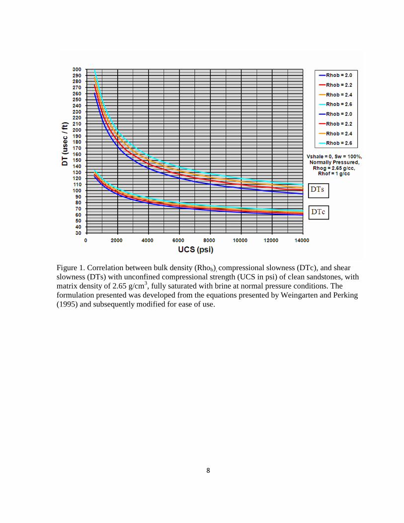
tests or estimated from well logs. Weingarten and Perkins (1995) presented useful correlations
of IFA and cohesion (Co) using acoustic slowness ( sec/ft) and bulk density (Rhob, g/cm3).
The correlations have been recast into a graphical expression (Figure 1) of UCS by
Page 16
8
Figure 1. Correlation between bulk density (Rhob), compressional slowness (DTc), and shear
slowness (DTs) with unconfined compressional strength (UCS in psi) of clean sandstones, with
matrix density of 2.65 g/cm3, fully saturated with brine at normal pressure conditions. The
formulation presented was developed from the equations presented by Weingarten and Perking
(1995) and subsequently modified for ease of use.
Page 17
9
. (Eq. 1)
To visualize the dependence of UCS on IFA, two times the trigonometric function in Equation
1 is displayed in Appendix 2 as “Cohesion to UCS Multiplier from Internal Friction Angle.”
In the laboratory, a convenient way to express the strength of rocks is to plot the axial
stress at failure on the ordinate, and confinement on the abscissa from two or more companion
samples subjected to triaxial compression test (Figure 2). A trend of increasing axial stress at
failure with increase in confinement is the normal response (Van der Pluijm and Marshak,
2004). As a reference regarding the span of UCS values, Table 2 presents a list of a few known
rock formations and associated UCS values.
Techniques such as indentation tests using a penetrometer with any one of assorted
point sizes and shapes, rebound “hammers” of various sizes with a wide range of impact
forces, and sonic devices with varying configurations are employed to determine rock strength.
One particularly useful point-stress penetrometer is a handheld micro-conical point indenter
referred to as the Dimpler (Figure 3). Its name refers to the small conical depression it creates
(Ramos et al., 2008). The shape and depth of the indentation are recorded by means of a dyed
conical tip that is impressed onto a compliant, removable tape affixed to the surface of interest.
In the case of core, the surface is first covered with compliant tape that is about a square inch
in size. The conical tip of the indenter is coated with a red dye and then forced, at a constant
axial stress, through the tape and into the sample creating a conical red depression (dimple) on
the tape. The combination of red dye and tape preserves a record of the dimple geometrical
attributes. The geometrical attributes (e.g. diameter and depth) depend on the rock UCS and
IFA (Ramos et al., 2008). The tape is then removed from the sample and placed on a flat
Page 18
10
Figure 2. Triaxial compression test geometry and a plot of axial stress at failure for a given
confinement from three separate triaxial tests of companion samples. Best fit line is projected
through the data points and extrapolated to the ordinate (zero confinement). The value at zero
confinement is referred to as the Unconfined Compressive Strength (UCS). The slope of the
best-fit extrapolated line (mbfexl) is related to the rock’s Internal Friction Angle (IFA) by
.
Page 19
11
Table 2: Collection of selected UCS values.
Rock UCS, psi, (~MPa) Source
Nevada Test Site tuff 1639 (11.3) Goodman, 1989
Cement (oilfield) ~100 (.68) to 6500 (44.8) Halliburton, 1978
Flaming Gorge shale 5100 (35.2) Goodman, 1989
Bedford limestone 7400 (51) Goodman, 1989
Berea sandstone 10700 (73.9) Goodman, 1989
Micaceous shale 10900 (75.2) Goodman, 1989
Barnett shale ~8000 (55.2) to 11000 (75.8) Enderlin, 2009, unpublished
Lockport dolomite 13100 (90.3) Goodman, 1989
James Lime (TX) ~7000 (48.3) to 15000 (103.4) Enderlin, 2009, unpublished
Nevada Test Site granite 20500 (141.4) Goodman, 1989
Navajo sandstone 31030 (214) Goodman, 1989
Solenhofen limestone 35500 (244.8) Goodman, 1989
Figure 3. Dimpler point penetrometer test.
Page 20
12
medium for archiving. The diameter of a dimple is measured with a graduated surface
magnifying glass. Correlation between dimple diameter and UCS from triaxial testing has been
established and is presented graphically in Figure 4 (Enderlin, 1998, unpublished).
Characterization of Stress Magnitude and Direction:
Overburden (SV):
In the approach presented, SV is the reference for SH and Sh. Therefore, SV needs to be
carefully determined. In most cases, SV is the stress exerted by the overburden above the point
of interest in the subsurface, and can be expressed as a function of the densities of earth
materials measured vertically from the surface to the point of interest. One approach is to sum
the log bulk density (Rhob, g/cm3) readings one depth increment at a time, between the surface
and the point of interest, then divide by the total number of depth increments used, obtaining
an average density value (avRhob) of the overburden. Multiplying the avRhob by 0.4335
psig/ftcm3 (14.7 psi stands 33.91 vertical feet of 1 g/cm
3 water) and the True Vertical Depth
(TVD, in feet) will yield an approximation of SV in psi. Care needs to be taken to ascertain that
the TVD log derived for the Measured Depth log (MD) is, in fact, equivalent in thickness and
density to the section directly above the point of interest. Another caveat is the nature of the
bulk density readings regarding the relationship between the “true density” and “calibrated
electron density” (apparent log density) as a function of the quotient of the atomic number (Z)
and atomic weight (A) (Schlumberger, 1972), where
(Eq. 2)
Page 21
13
Figure 4. Correlation between the diameter of a dimple, measured in “ticks,” (each tick is equal
to 0.005 of an inch) and the UCS of the sample in psi (Enderlin, 1998, unpublished).
Page 22
14
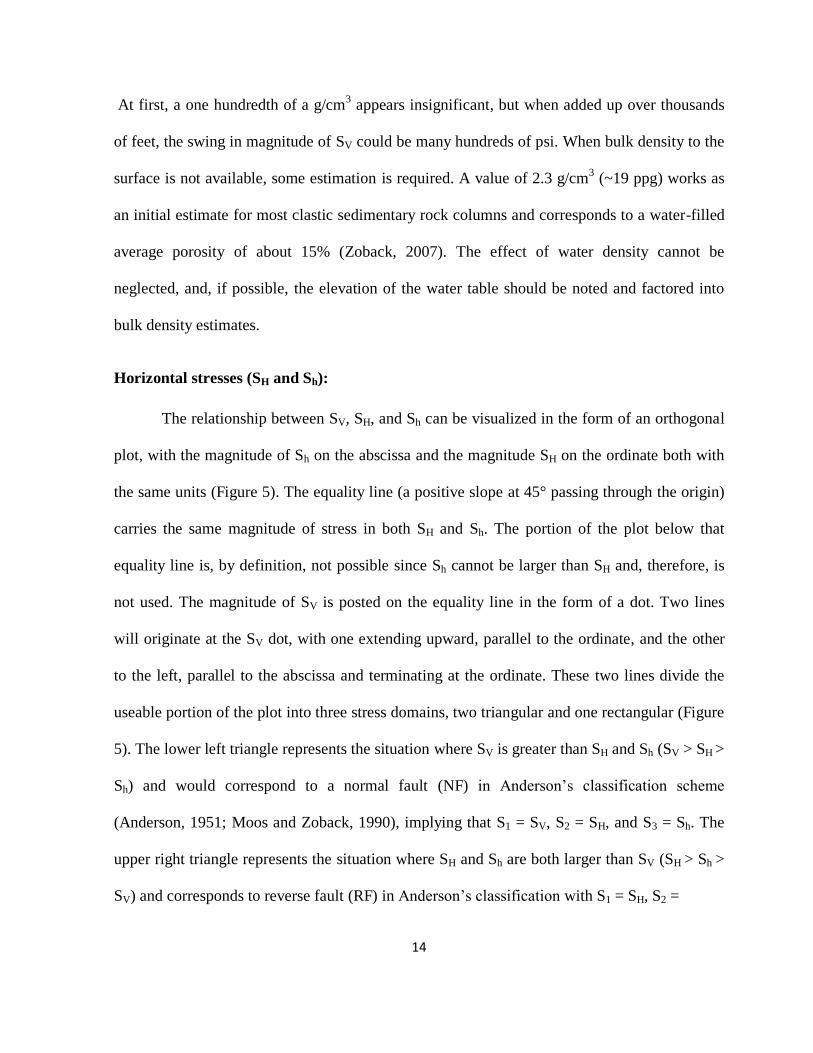
At first, a one hundredth of a g/cm3 appears insignificant, but when added up over thousands
of feet, the swing in magnitude of SV could be many hundreds of psi. When bulk density to the
surface is not available, some estimation is required. A value of 2.3 g/cm3 (~19 ppg) works as
an initial estimate for most clastic sedimentary rock columns and corresponds to a water-filled
average porosity of about 15% (Zoback, 2007). The effect of water density cannot be
neglected, and, if possible, the elevation of the water table should be noted and factored into
bulk density estimates.
Horizontal stresses (SH and Sh):
The relationship between SV, SH, and Sh can be visualized in the form of an orthogonal
plot, with the magnitude of Sh on the abscissa and the magnitude SH on the ordinate both with
the same units (Figure 5). The equality line (a positive slope at 45° passing through the origin)
carries the same magnitude of stress in both SH and Sh. The portion of the plot below that
equality line is, by definition, not possible since Sh cannot be larger than SH and, therefore, is
not used. The magnitude of SV is posted on the equality line in the form of a dot. Two lines
will originate at the SV dot, with one extending upward, parallel to the ordinate, and the other
to the left, parallel to the abscissa and terminating at the ordinate. These two lines divide the
useable portion of the plot into three stress domains, two triangular and one rectangular (Figure
5). The lower left triangle represents the situation where SV is greater than SH and Sh (SV > SH >
Sh) and would correspond to a normal fault (NF) in Anderson’s classification scheme
(Anderson, 1951; Moos and Zoback, 1990), implying that S1 = SV, S2 = SH, and S3 = Sh. The
upper right triangle represents the situation where SH and Sh are both larger than SV (SH > Sh >
SV) and corresponds to reverse fault (RF) in Anderson’s classification with S1 = SH, S2 =
Page 23
15
Figure 5. Plot of SH versus Sh with the equality line and fault boundaries displayed. The
location of SV on the equality line is the singularity of normal fault, strike-slip and reverse fault
stress domains as defined by Anderson (1951). Also presented are the appropriate association
with S1, S2, and S3.
Page 24
16
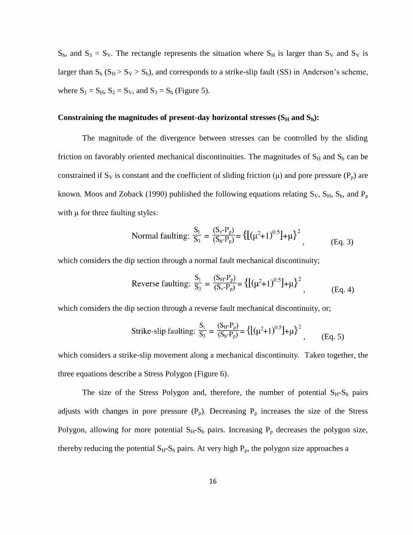
Sh, and S3 = SV. The rectangle represents the situation where SH is larger than SV and SV is
larger than Sh (SH > SV > Sh), and corresponds to a strike-slip fault (SS) in Anderson’s scheme,
where S1 = SH, S2 = SV, and S3 = Sh (Figure 5).
Constraining the magnitudes of present-day horizontal stresses (SH and Sh):
The magnitude of the divergence between stresses can be controlled by the sliding
friction on favorably oriented mechanical discontinuities. The magnitudes of SH and Sh can be
constrained if SV is constant and the coefficient of sliding friction (μ) and pore pressure (Pp) are
known. Moos and Zoback (1990) published the following equations relating SV, SH, Sh, and Pp
with μ for three faulting styles:
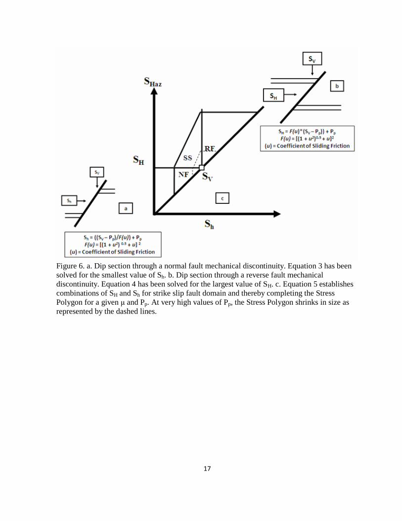
, (Eq. 3)
which considers the dip section through a normal fault mechanical discontinuity;
, (Eq. 4)
which considers the dip section through a reverse fault mechanical discontinuity, or;
, (Eq. 5)
which considers a strike-slip movement along a mechanical discontinuity. Taken together, the
three equations describe a Stress Polygon (Figure 6).
The size of the Stress Polygon and, therefore, the number of potential SH-Sh pairs
adjusts with changes in pore pressure (Pp). Decreasing Pp increases the size of the Stress
Polygon, allowing for more potential SH-Sh pairs. Increasing Pp decreases the polygon size,
thereby reducing the potential SH-Sh pairs. At very high Pp, the polygon size approaches a
Page 25
17
Figure 6. a. Dip section through a normal fault mechanical discontinuity. Equation 3 has been
solved for the smallest value of Sh. b. Dip section through a reverse fault mechanical
discontinuity. Equation 4 has been solved for the largest value of SH. c. Equation 5 establishes
combinations of SH and Sh for strike slip fault domain and thereby completing the Stress
Polygon for a given μ and Pp. At very high values of Pp, the Stress Polygon shrinks in size as
represented by the dashed lines.
Page 26
18
singularity (SV), where normal faults, strike-slip faults, and reverse faults can exist
simultaneously (Figure 6).
Setting the magnitudes of Sh via classical methods:
Based on Poisson’s ratio (v), SV, and Pp, Eaton (1969) suggested a technique for the
determination of Sh, where
. (Eq. 6)
This technique has been elaborated by Gretner (1981) and Cumella and Scheevel (2008), who
include the concept of strain and Young’s modulus in the formulation.
Another method for determining the value of Sh is to produce a Mode I tensile fracture
originating at the borehole wall by increasing the pressure within the borehole until the rock
fails. In this case, the borehole wall acts as the free surface and a Mode I fracture forms.
Analysis and interpretation of the pressure to initiate, propagate, and, once the pumping stops,
the closing of the fracture (“closure pressure”) can be used to evaluate the magnitude of Sh. All
these analyses assume that a Mode I fracture was induced and no reactivation of pre existing
mechanical discontinuities took place. The processes for inducing an assumed Mode I fracture
go by many names including Leak Off Test (LOT, performed between setting casing and
continued drilling), mini-fracture test, and fracture stimulation (Zoback, 2007). Unfortunately,
in most cases, the values of LOT and “closure pressure” are reported, but information about the
method of analysis or insights into the quality of the data are rarely available.
Page 27
19
Setting the magnitudes of SH and Sh utilizing stress related borehole failures and the
Stress Polygon:
A borehole can be viewed as a stress magnifier. The stresses supported by rock before
being removed by the bit are relocated and concentrated at the borehole wall. The concentrated
stresses around the borehole are referred to as “hoop” stresses. For a vertical, cylindrical
borehole, the magnitude of concentrated stress has been described by the Kirsch equations
(Kirsch, 1898; Jaeger and Cook, 1979). A simplified expression for the largest magnitude of
effective hoop (MaxHoop) stress concentration at the borehole wall is:
effective MaxHoop stress = 3SH – Sh - 2Pp - (Pm - Pp) (Eq. 7)
where Pm equals the stress exerted by the fluids in the borehole. For the smallest magnitude of
effective hoop (MinHoop), stress concentration at the borehole wall is:
effective MinHoop stress = 3Sh - SH - 2Pp - (Pm - Pp) (Eq. 8)
If Pp and Pm are held constant then the above relationships reduce to
effective MaxHoop stress = 3SH - Sh - Constant (Eq. 9)
and
effective MinHoop stress = 3Sh - SH - Constant (Eq. 10)
This implies that for every SH-Sh pair on the Stress Polygon, the value of effective MaxHoop
stress can be determined and contours of equal stress can be plotted on the Stress Polygon
(Figure 7). Where the effective MaxHoop stress exceeds the strength of the rock along the
borehole wall, the rock fails in shear and pieces of rock (cavings) fall into the borehole, thereby
enlarging the borehole size and leaving behind “breakouts”. Such borehole enlargements are
observable via open-hole logs, such as calipers, as a borehole diameter becomes larger than bit
size (Plumb and Hickman, 1985) and, depending on the vertical scale, as dark spots or stripes
Page 28
20
Figure 7. Contours of equal effective MaxHoop stress (in psi) as mapped on the Stress
Polygon. Potential SH – Sh combinations are restricted by the presence or absence of breakouts
for a rock that can just withstand 6000 psi (41.3 MPa) of stress before failing.
Page 29
21
on borehole image logs. For example, if a rock can withstand 6000 psi of stress before failure,
then observation of the presence or absence of breakouts partitions the possible SH-Sh pairs that
can exist at the 6000 psi contour line (Figure 7). If no breakouts are observed, then present-day
stress state is below the 6000 psi contour line. On the other hand, the existence of breakouts
indicates that the present-day stress state is above the 6000 psi contour line.
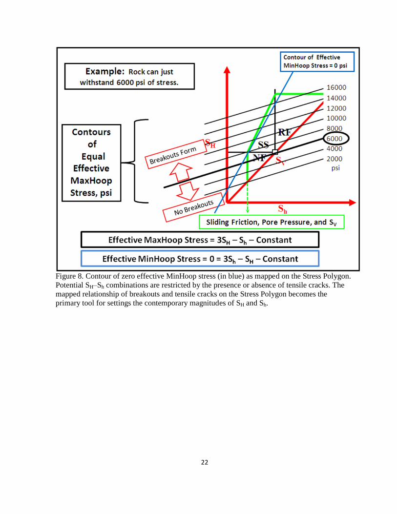
In the same manner, for every SH-Sh pair on the Stress Polygon, the value of effective
MinHoop stress can be determined and contours of equal stress can be constructed. If the
effective MinHoop stress exceeds the tensile strength of the rock, a Mode I tensile fracture may
develop. Since the span of tensile strength of rocks is much smaller than compressional
strength, only the 0 stress contour is plotted on the Stress Polygon (Figure 8). Just as with
breakouts, the presence or absence of tensile cracks partitions the possible SH-Sh pairs that exist
at the 0 psi contour line. Although the presence or absence of tensile cracks is best determined
by analysis of borehole image logs, inferences can be made from analysis of drilling data such
as “flow in – flow out”. If tensile cracks are not observed, then present-day stress state is to the
right of the 0 psi contour line. On the other hand, the existence of induced tensile fractures
suggests that present-day stress state is to the left of the 0 psi contour line (Figure 8).
Combining the effective MaxHoop stress with the effective MinHoop stress on the same Stress
Polygon is the primary tool for setting the magnitudes of SH and Sh (Figure 8).
Determining the direction of SH (SHaz):
One approach for resolving the direction of SH (SHaz) is to consider the Stress Polygon
in map view. In such a view, we assume SV to be vertical and the SH axis (ordinate) to be a
reference direction (Figure 9). Further, consider the boundaries of the Stress Polygon, less the
Page 30
22
Figure 8. Contour of zero effective MinHoop stress (in blue) as mapped on the Stress Polygon.
Potential SH–Sh combinations are restricted by the presence or absence of tensile cracks. The
mapped relationship of breakouts and tensile cracks on the Stress Polygon becomes the
primary tool for settings the contemporary magnitudes of SH and Sh.
Page 31
23
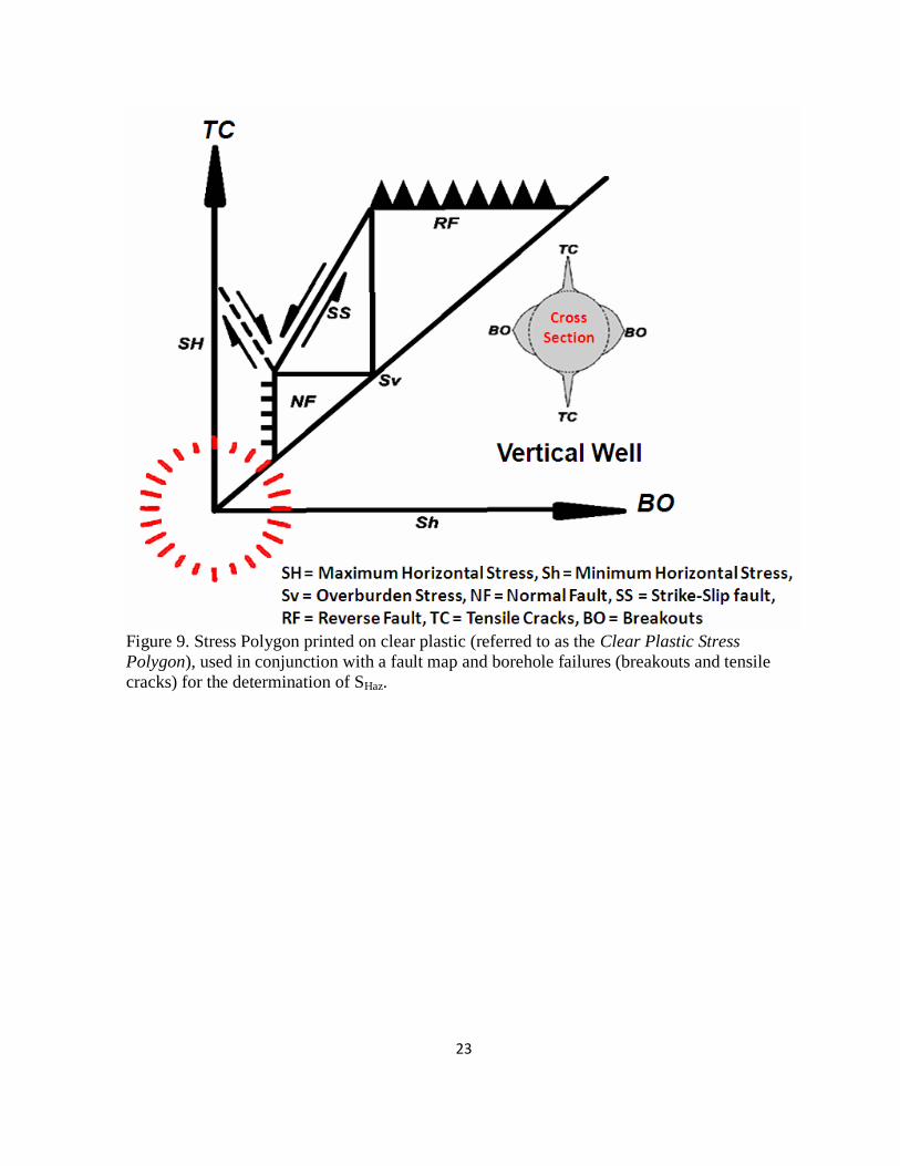
Figure 9. Stress Polygon printed on clear plastic (referred to as the Clear Plastic Stress
Polygon), used in conjunction with a fault map and borehole failures (breakouts and tensile
cracks) for the determination of SHaz.
Page 32
24
equality line, as the strike for the associated fault (normal fault = NF, strike-slip fault = SS, and
reverse fault = RF). Printing the Stress Polygon on a clear plastic sheet (referred to as a Clear
Plastic Stress Polygon) facilitates use with existing structure maps. Placing the Clear Plastic
Stress Polygon over a structure map of nearby active faults, so that the appropriate polygon
strike boundary is aligned parallel to the strike of the mapped faults, results in the SH axis
pointing in the direction (map coordinates) of SH. SHaz can be read directly with respect to
geographic north via the red angular index (Figure 9).
Another method for determining SHaz is to observe the heading of tensile cracks (TC)
and/or breakouts (BO) on an image log. If tensile cracks and breakouts are observed, then SHaz
is in the direction of tensile cracks and Sh in the direction of breakouts. The same orientation
relationship is noted on the cross section insert of Figure 9 and at the arrow end of both stress
axes.
To illustrate the quantitative aspects of the stress polygon two examples will be used.
The example 1 is a continuation of Figures 7 and 8 (unstated pore pressure, coefficient of
sliding friction (μ), SHaz and stress units) but includes a cartoon of borehole images. Example 2
extends the concepts with realistic values for all variables.
Example 1
For a vertical well, if breakouts and tensile cracks are found in a rock able to withstand
6000 psi, then present-day magnitudes of SH and Sh can be constrained (Figure 10). In this
case, the SH-Sh pair is above the 6000 psi (41.3 MPa) MaxHoop stress contour line and to the
left of the 0 psi MinHoop stress contour line and resides within the borders of the Stress
Page 33
25
Polygon as determined from sliding friction, pore pressure and SV. Experience indicates that
choosing the lower magnitudes for SH and Sh that accommodate the observation is a reasonable
Figure 10. Determining SH and Sh magnitudes (yellow ellipse) by observing (1) that a rock
capable of just withstanding 6000 psi (41.3 MPa) of stress before failing forming breakouts and
(2) tensile cracks have formed. The breakouts are recognized and orientation observed (with
respect to N, E, S, and W) in the uppermost of the two borehole image inserts on the left (the
two dark spots). The lower borehole image shows tensile fractures as dark irregular vertical
streaks. SH1 and Sh1 are the selected values of stress.
Page 34
26
first estimation of the stress state (yellow spot in the strike-slip domain on Figure 10). The
estimated values of SH1 and Sh1 may be thus selected. Since the breakouts in Figure 10 are east-
southeast to west-northwest trending and tensile cracks are trending north-northeast to south-
southwest, SHaz is oriented north-northeast to south-southwest. Hence, the characterization of
present-day state of stress is determined and SHaz is approximately 030° (N30°E). Since the
stress state resides in the strike-slip stress domain, then S1 = SH1, S2 = SV, and S3 = Sh1.
Example 2
For the following discussion on magnitudes of the normal stress and shear stress acting on an
arbitrarily oriented planar mechanical discontinuity, all appropriate variables need to be
assigned practical numeric values. To that end, Example 2 is offered and displayed as a Stress
Polygon (Figure 11). Compared to the Stress Polygon for Example 1 (Figure 10), the 6000
UCS psi (41.3 MPa) strength contour has moved down on the Stress Polygon. This is because
of the greater depth, mud weight (Pm), and pore pressure (Pp) values in this example. The
values at approximately 8000 ft (2438 m) True Vertical Depth (TVD) are posted in Table 3.
The orientation of the planar mechanical discontinuity can be described by its strike and dip.
Normal and Shear Stress Magnitudes Acting on an Arbitrarily Oriented Planar
Mechanical Discontinuity:
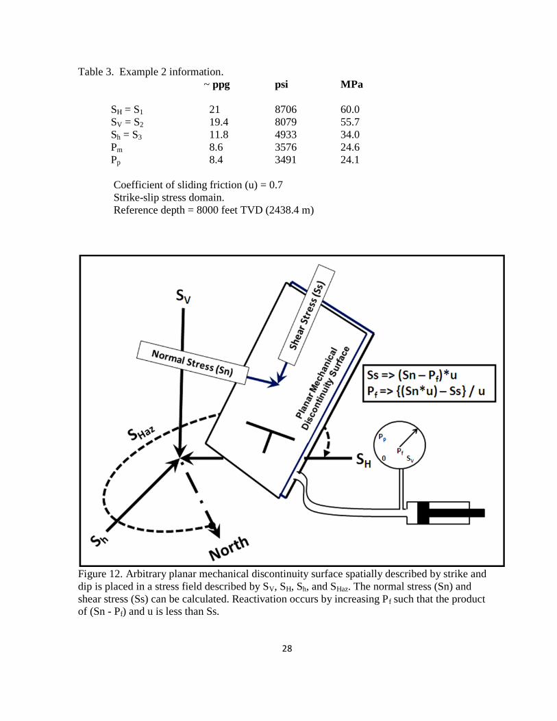
Having estimated the state of present-day stress (Table 3), the magnitudes of the normal
stress and shear stress acting on an arbitrarily oriented planar mechanical discontinuity can be
estimated (Figure 12).
Page 35
27
Figure 11. Stress Polygon with four rock strength contour lines and their UCS values plotted.
The yellow rock strength lines are positioned, for reference only, along the equality line, one
through SV (dark red dot), one half-way between SV and the lower left end of the equality line,
and last one halfway between SV and the upper right end of the equality line. The red line and
associated value box corresponds to the estimated rock strength of interest (6000 psi: 41.3
MPa). The blue dot marks the estimated present-day state of stress.
Page 36
28
Table 3. Example 2 information.
~ ppg psi MPa
SH = S1 21 8706 60.0
SV = S2 19.4 8079 55.7
Sh = S3 11.8 4933 34.0
Pm 8.6 3576 24.6
Pp 8.4 3491 24.1
Coefficient of sliding friction (u) = 0.7
Strike-slip stress domain.
Reference depth = 8000 feet TVD (2438.4 m)
Figure 12. Arbitrary planar mechanical discontinuity surface spatially described by strike and
dip is placed in a stress field described by SV, SH, Sh, and SHaz. The normal stress (Sn) and
shear stress (Ss) can be calculated. Reactivation occurs by increasing Pf such that the product of (Sn - Pf) and u is less than Ss.
Page 37
29
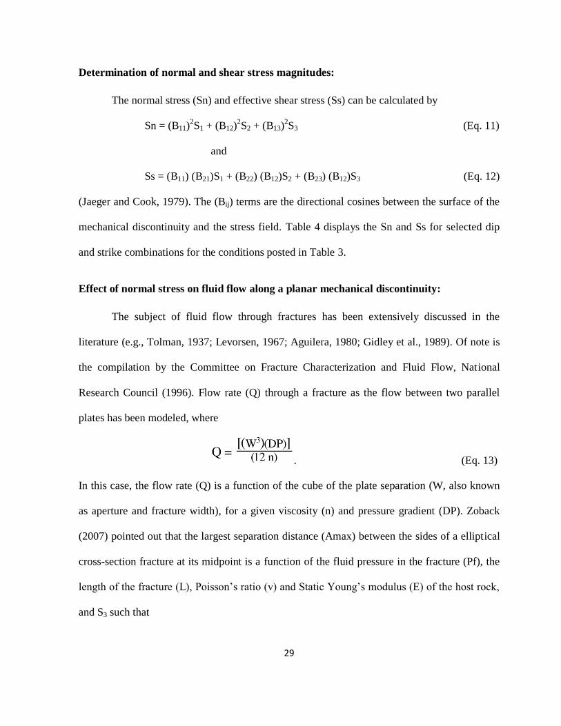
Determination of normal and shear stress magnitudes:
The normal stress (Sn) and effective shear stress (Ss) can be calculated by
Sn = (B11)2S1 + (B12)
2S2 + (B13)
2S3 (Eq. 11)
and
Ss = (B11) (B21)S1 + (B22) (B12)S2 + (B23) (B12)S3 (Eq. 12)
(Jaeger and Cook, 1979). The (Bij) terms are the directional cosines between the surface of the
mechanical discontinuity and the stress field. Table 4 displays the Sn and Ss for selected dip
and strike combinations for the conditions posted in Table 3.
Effect of normal stress on fluid flow along a planar mechanical discontinuity:
The subject of fluid flow through fractures has been extensively discussed in the
literature (e.g., Tolman, 1937; Levorsen, 1967; Aguilera, 1980; Gidley et al., 1989). Of note is
the compilation by the Committee on Fracture Characterization and Fluid Flow, National
Research Council (1996). Flow rate (Q) through a fracture as the flow between two parallel
plates has been modeled, where
. (Eq. 13)
In this case, the flow rate (Q) is a function of the cube of the plate separation (W, also known
as aperture and fracture width), for a given viscosity (n) and pressure gradient (DP). Zoback
(2007) pointed out that the largest separation distance (Amax) between the sides of a elliptical
cross-section fracture at its midpoint is a function of the fluid pressure in the fracture (Pf), the
length of the fracture (L), Poisson’s ratio (v) and Static Young’s modulus (E) of the host rock,
and S3 such that
Page 38
30
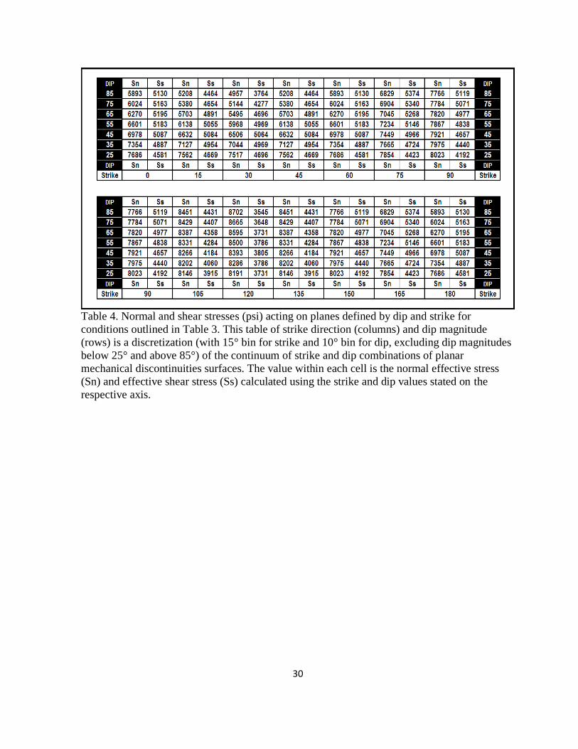
Table 4. Normal and shear stresses (psi) acting on planes defined by dip and strike for
conditions outlined in Table 3. This table of strike direction (columns) and dip magnitude
(rows) is a discretization (with 15° bin for strike and 10° bin for dip, excluding dip magnitudes
below 25° and above 85°) of the continuum of strike and dip combinations of planar
mechanical discontinuities surfaces. The value within each cell is the normal effective stress
(Sn) and effective shear stress (Ss) calculated using the strike and dip values stated on the
respective axis.
Page 39
31
. (Eq. 14)
This indicates the dependence of aperture on the magnitude of S3, which controls flow rate (Q)
as described by
. (Eq. 15)
Thus, the flow rate through a fracture responding to a pressure gradient will be proportional to
the cube of the product of fracture length (L) times the difference between the fluid pressure
(Pf) inside the fracture and S3. That is, the fluid pressure (Pf) inside the fracture is trying to
open the fracture, while S3 is trying to close the fracture.
Aguilera (1980) cast the flow through fractures in terms of permeability (Kf in Darcy)
as
Kf = (54 X 106) W
2, (Eq. 16)
where W (fracture width, fracture aperture) is in inches. Consequently, the flow rate through a
fracture is proportional to the cube of the aperture responding to S3 (Equation 13), where
fracture permeability is proportional to the square of the aperture responding to S3 (Equation
16). For reference, Aguilera (1980) pointed out that the average permeability, or “system
permeability,” of 13510 millidarcy (md) results when a 1 md rock with dimensions of one
cubic foot (1 ft3) contains three fractures each with an aperture of 0.01 of an inch. Fractures
make a great difference in system permeability. It is the fracture’s aperture, responding to
stress, that controls the magnitude of that difference.
Bandis et al. (1983) illustrated, through laboratory experiments, that fracture aperture is
controlled by stress normal to the fracture. Stress of 3000 psi (20.6 MPa) normal to a fracture
Page 40
32
surface will reduce the initial aperture by 40% with one stressing cycle. After three cycles of
stressing the aperture is reduced by approximately 60%. Gutierrez et al. (2000) completed a
series of laboratory experiments on shales and documented that stress of 1450 psi (10 MPa)
normal to a fracture surface will reduce the initial permeability by 90%. Stress can degrade
fracture permeability even if one places propping agents in the fracture aperture. Gidley et al.
(1984) demonstrated that a fracture packed with propping agents experienced a substantial loss
of permeability due to grain crushing, embedment, and subsequent development and migration
of fines when exposed to normal stress above 3000 psi (20.6 MPa) to 4000 psi (27.6 MPa). In
summary, normal effective stresses above 2000 psi (13.7 MPa) to 3000 psi (20.6 MPa) can
significantly discourage the ability of a fracture to allow fluids to flow along the surface.
Effect of shear stress on fluid flow along a planar mechanical discontinuity:
In a situation where the host rock permeability is much less than 0.001 md, the pressure
within the mechanical discontinuity (Pf) can be different than the pore pressure (Pp) of the host
rock (i.e., low leak off). A planar mechanical discontinuity oriented within a stress field
defined by SV, SH, Sh, and SHaz (as depicted in Figure 12), will fail in shear (Mode II or Mode
III) when the magnitude of the shear stress (Ss) is greater than the product of the coefficient of
sliding friction (μ) and the normal stress (Sn) less the pressure within the mechanical
discontinuity (Pf),
Ss > μ (Sn – Pf). (Eq. 17)
Such shear failure results in sliding along the surface and subsequent dilation (opening) due to
riding up on asperities positioned along the surface (Barton et al., 1985). Such a state of shear
failure is recognized as a “critically stressed” situation, although the term reactivation is
Page 41
33
preferred here. Barton et al. (1995) recognized that fluid flow is encouraged along reactivated
faults; a principle that was subsequently extended to fractures by Zoback (2007) and is
corroborated by personal experience.
Considering the relationship
Ss = μ (Sn – Pfr) (Eq. 18)
such that Pfr is the pressure within the mechanical discontinuity (not Pp) which will be
responsible for the initiation of reactivation. Solving for Pfr, the relationship
(Eq. 19)
is obtained. Therefore, for a given set of Sn, Ss, and μ, the Pfr can be calculated.
In the previous section, estimates of Sn and Ss were obtained for a surface described by
strike and dip. Following the same logic, one can now calculate Pfr for a given coefficient of
sliding friction (μ) for any strike-dip combination. Results of such calculations using
parameters of Example 2 (Table 3) are presented in Table 5 in the same discretized strike and
dip format as Table 4. In this case, the lowest value of Pfr occurs in two places, strike of 0° and
dip of 85°, and strike of 60° with dip of 85°. Thus, if fractures with these orientations exist,
they would be more apt to encourage fluid flow along their surfaces than other strike-dip
combinations.
Worth noting is the phenomenon that once a mechanical discontinuity has been
reactivated, the “fall-off” pressure response to the process of “deactivation” should not be
misconstrued as “closure pressure” associated with a value for Sh from a linear elastic Mode I
fracture. Couzens-Schultz and Chan (2010) present a field study demonstrating the potential
confusion.
Page 42
34
Table 5. The value in each cell represents the pressure (Pfr in psi) within a fault, fracture,
crack, bedding plane surface required to reactivate and fail in shear at the posted strike and dip
values. Values assume constant coefficient of sliding friction (u) of 0.7 (posted in the lower
most left cell) and zero cohesion. Color code is as follows: Yellow: Required pressure for
reactivate that is less than Sh.; Blue: Reactivate at pressures that are greater than Sh; Red:
Reactivation pressure less than mud pressure.
Page 43
35
Given the influence on fluid flow that stress normal to the discontinuity commands, the
effectiveness and preservation potential of shear-induced dilation along a discontinuity can be
evaluated by combining the reactivation pressure and the normal stress acting on that
discontinuity. Table 6 represents such a combination by taking the average of the effective,
reactivation pressure (removing the influence of pore pressure) and the effective normal
stresses as a function of strike and dip. Such a combination can shift the orientation of the most
likely for preservation from the orientation of the most likely for reactivation (Table 5).
Summary
I have presented a methodology for evaluating the potential for flow along the surfaces
of mechanical discontinuities (faults and fractures) as a function of reactivation. The approach
is to first describe the rock strength, then characterize the present-day stresses. Next, one
establishes the normal and shear stresses acting on surfaces of mechanical discontinuities that
are described spatially by strike and dip. This is followed by determining the pressure
magnitude within each surface required to initiate reactivation. Finally, one has to review the
magnitude of pressure sources such as pore pressure, drilling fluids, completion fluids, and
injection fluids with respect to the reactivation pressures. If any of the sources exceeds the
reactivation pressure for a particular strike and dip, then fractures in that orientation are prone
to reactivate and allow fluids to flow along their surfaces.
Page 44
36
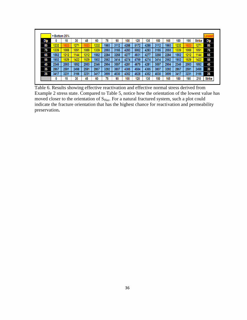
Table 6. Results showing effective reactivation and effective normal stress derived from
Example 2 stress state. Compared to Table 5, notice how the orientation of the lowest value has
moved closer to the orientation of SHaz. For a natural fractured system, such a plot could
indicate the fracture orientation that has the highest chance for reactivation and permeability
preservation.
Page 45
37
LABORATORY FLOW EXPERIMENT
Introduction:
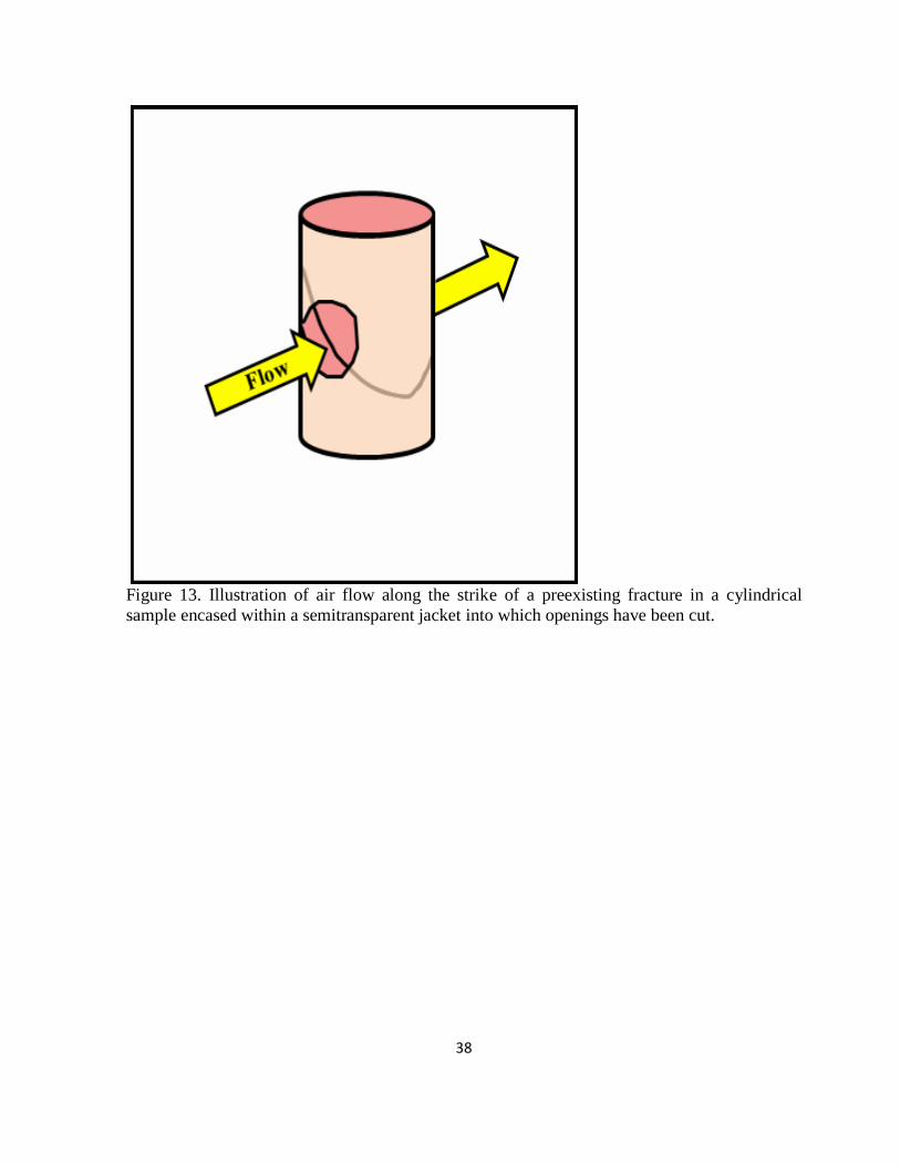
A series of experiments, which monitored the flow of dry air as a function of stress
along the strike of preexisting fractures in a cylindrical sample of Berea Sandstone (Figure 13)
were conducted at ConocoPhillips’ Rock Mechanics Laboratories in Bartlesville Oklahoma.
The object of the experiments was to set up a laboratory experiment which would emulate the
presented methodology and duplicate the field observations of Barton et al. (1995) that
associated fluid flow with reactivation along preexisting mechanical discontinuities. The flow
rate was monitored as the confining and axial stresses were increased through reactivation.
Procedure:
A cylindrical sample was extracted from a block of Berea Sandstone, which has a
permeability to air of approximately 300 millidarcy and a porosity of roughly 20%. After
trimming the ends square, the approximately 1 inch (2.54 cm) in diameter and 2 inches (5.08
cm) long sample was placed into a Teflon jacket (Figure 14). The sample was then positioned
in a cell so that confining stress could be applied and the sample pore pressure could be vented
to the atmosphere (drained test). Placing the confining cell in a stiff loading system (Figure
15), allowed application of axial stress and established the triaxial loading system.
Subsequently, the sample was subjected to an increase of axial stress from 1300 psi (9 MPa) to
13157 psi (90.7 MPa) at room temperature and a constant confining stress of 1000 psi (6.9
MPa). Applying axial stress of 13157 psi (90.7 MPa) just exceeded the strength of the rock
(Ultimate Strength) and induced failure, which resulted in the formation of a set of conjugate
Page 46
38
Figure 13. Illustration of air flow along the strike of a preexisting fracture in a cylindrical
sample encased within a semitransparent jacket into which openings have been cut.
Page 47
39
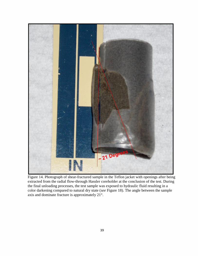
Figure 14. Photograph of shear-fractured sample in the Teflon jacket with openings after being
extracted from the radial flow-through Hassler coreholder at the conclusion of the test. During
the final unloading processes, the test sample was exposed to hydraulic fluid resulting in a
color darkening compared to natural dry state (see Figure 18). The angle between the sample
axis and dominate fracture is approximately 21°.
Page 48
40
Figure 15. TerraTek 375 ton stiff loading system used for the experiment.
Page 49
41
shear fractures (Figure 14). Throughout the experiment, stress and strain data were recorded
(Figure 16).
After failure, the rock sample was removed from the triaxial loading system. Two
openings, aligned along the strike of the induced fractures, were cut into the Teflon jacket
(Figure 14). The jacketed sample was placed in a radial flow-through Hassler coreholder
(Figure 17a) with the ports of the coreholder aligned with the openings in the Teflon jacket and
strike of the fracture. The sample was then repositioned in the triaxial loading system (Figure
17b). With a constant up-stream pressure of 56 psi (0.38 MPa), the flow rate of dry air at room
temperature was continually monitored with an Agilent AMD2000 digital flow meter as the air
passed through the radial flow-through Hassler coreholder and the fractured sample before
venting to the atmosphere. Under normal circumstances flow rate should have been recorded,
in milliliter per minute (mL/min), via a RS232 interface every 4.9 seconds throughout the 16
hour stressing. Unfortunately, a persistent problem would randomly halt the flow data from
being recorded and required a manual restart. As a result there are numerous intervals of
missing flow data (Figure 18).
Initially the confining stress on the sample was brought to 494 psi (3.4 MPa), while the
axial stress was increased to about 700 psi (4.8 MPa). Around hour 18.5 of system elapsed
time, the axial stress was increased, under strain control, at a rate of 0.1 % strain per hour and
continued at that rate for the next 10 hours except for a hold period between hour 22 and 23. At
hour 28.65, unloading started and continued to hour 34 (Figure 18).
Page 50
42
Figure 16. Stress strain record for the initial failure
Page 51
43
Figure 17a. Radial flow-through Hassler coreholder.
Figure 17b. Radial flow-through Hassler coreholder positioned in the
triaxial compression loading configuration.
Page 52
44
Figure 18.Data from flow test.
Page 53
45
Discussion:
In much the same manner that UCS can be calculated from cohesion and internal
friction angle (Eq. 1), UCS can also be estimated from a single triaxial test taken to failure
using the effective confinement (Sc’), which is confining stress less the pore pressure, Ultimate
Strength (US), and internal friction angle (IFA) in the following manner
(Eq. 20)
For reference, the last part of Equation 20
(
is presented in Appendix 2 as “Confinement Multiplier from Internal Fraction Angle”. The IFA
can be estimated from the angle that forms between the axial stress and the plane which best
describes the rock failure (ARF) such that
. (Eq. 21)
For the sample in the experiment, ARF is approximately 21° (Figure 14) resulting in an IFA
estimate of 48°. With US equal to 13157 psi (90.7 MPa) (Figure 16) and Sc’ approximately
1000 psi (6.9 MPa), a UCS of 6300 psi (43.4 MPa) is calculated. Dimple analyses of the
companion block of Berea Sandstone from which the test sample was extracted resulted in
dimple diameters of 6 ticks (Figure 19), which suggest a UCS of approximately 5500 psi (37.9
MPa) (Figure 4). These two UCS values are in reasonable agreement. Dimple analyses of the
test sample after the conclusion of the experiment resulted in dimple diameters of 10 ticks
(Figure 18), which correlate with an UCS of approximately 2100 psi (14.5 MPa) (Figure 4).
These measurements illustrate the effects of recently imbibed fluids, especially oil, on the
analyses.
Page 54
46
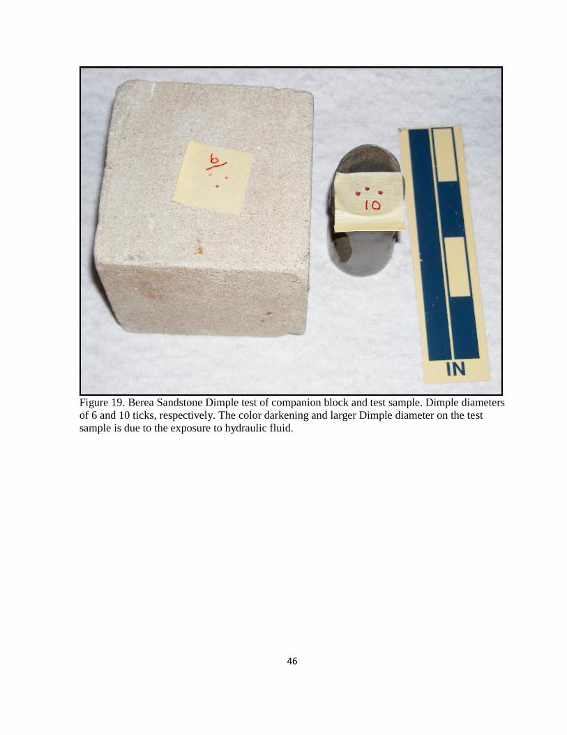
Figure 19. Berea Sandstone Dimple test of companion block and test sample. Dimple diameters
of 6 and 10 ticks, respectively. The color darkening and larger Dimple diameter on the test
sample is due to the exposure to hydraulic fluid.
Page 55
47
With the axial stress vertical, the confining stress is equal to the horizontal stresses (Sh
and SH). Furthermore, since the axial stress within the triaxial loading cell is greater than
confining stress, a normal fault condition persists. Since Sh and SH are the same, the stress state
of the sample within the cell lies on the equality line for the representative Stress Polygon
(Figure 20).
With ARF equal to 21° and the axial stress being vertical, the plane which best
describes the rock failure dips 69°. Using the method described earlier (see section “Normal
and Shear Stresses Magnitudes Acting on an Arbitrarily Oriented Planar Mechanical
Discontinuity”) applied confining and axial stresses (Figure 18) are used to calculate both the
normal (Sn) and shear (Ss) stresses acting on the plane dipping 69°. Reviewing the axial stress
and strain curves (Figure 18), the axial stress curve starts to flatten between hour 24.7 and hour
25.3. Such a marked change of slope of the axial stress in a strain controlled experiment
suggests slip movement (reactivation) along the fracture(s). Solving for coefficient of sliding
friction (μ) in Equation 18 renders
μ = Ss / (Sn – Pfr) (Eq. 22)
where Sn and Ss are the normal and shear stresses, respectively, acting on the fracture surface,
and Pfr is the pressure within the mechanical discontinuity. At low injection (flow) rates Pfr is
equal to pore pressure in a permeable rock. Using the normal and shear stress conditions for
hour 25 of the experiment (Figure 21) and a Pfr equal to 25 psi (0.17 MPa), a μ of
approximately 1.41 is obtained. Similar calculations for reactivation pressures can be
performed for all time increments of the experiment (Table 7). For example at hour 24 with a μ
Page 56
48
Figure 20. (a.) Stress Polygon representing the stress state within the stress cell at hour 25
using an anticipated μ of 0.6 derived from UCS (6300 psi) and Figure 21. In order to use the
analysis tools available, it was necessary to emulate the conditions within the stress cell as a
well drilled in an area that has a Sv gradient very close to 1 psi/ft and a pore pressure relative
close to zero. Note that the stress state (blue dot) is outside the polygon suggesting a non-
natural condition. Further note that the polygon is rather large due from the low pore pressure.
(b) In order to get the stress state close to the polygon boundary a μ of 1.41 is necessary, which
significantly increases the polygon. (c) Illustrates the Normal Fault section of (b) with the
stress states posted for hour 20 and 22 along with hour 25 to help visualize the change of stress
state through the first half of stressing cycle.
Page 57
49
Figure 21. Flow data with axial stress and calculated normal and shear stresses acting on the
fracture dipping at 69°.
Table 7. As in Table 5, this table reflects the reactivation pressure (psi) for hour 25 stress
conditions using a μ = 1.41. Since SH = Sh, directionality is lost and all strikes have the same
value. In the stress cell, the fracture is dipping approximately 69°, which is not directly posted,
the reactivation pressure resides between 90 psi (for 65° of dip) and 15 psi (for 75° of dip).
Performing the calculation using Equations 11, 12, and 19 for a dip of 69° results in a value of
25 psi (0.17 MPa)
Page 58
50
equal to 1.41 the reactivation pressure is 65 psi (0.45 MPa) (Table 8) which is 40 psi higher
that that a hour 25. Interestingly, a μ of 1.41 appears high for rock strength of 6300 psi UCS
where the expected values are in the range of μ equal to approximately to 0.6 (Figure 22). The
two-fold increase in the coefficient of sliding friction most likely reflects the combined
stiffening influence of the Teflon jacket, Hassler coreholder, and “end effects” on a relative
small test sample.
At the beginning of the loading sequence, at hour 19, the dry air flow rate (Figure 18,
21, 23, and Appendix 1) averaged approximately 0.37 mL/min, while the flow rate decreased
to approximately 0.28 mL/min near the end of the loading sequence at hour 34. During the
intervening fifteen hours, the flow rate decreased by 24% as 4.2% strain occurred. 4.2% strain
translates to 0.084 inch (0.2 cm) of displacement. The most abrupt decrease in flow rate
occurred at hour 26.
The character of the flow rate seems to be associated with strain and changes in shear
and normal stress acting on the fracture surfaces. Between hour 19 and hour 20, when the
normal stress acting on the fracture surface is greater than the shear stress, the flow rate
fluctuated symmetrically by plus or minus 0.09 mL/min around the average value of 0.37
mL/min, although the fluctuations appear to occur randomly with time (Figure 23a). Once the
shear and normal stress were about equal, between hour 20 and hour 21, the flow rate
fluctuated asymmetrically about 0.37 mL/min, with the majority of the excursions lower than
0.37 mL/min (Figure 23b). When the shear stress exceeded the normal stress at about hour 21,
the character of the flow rate changed to an organized cyclic pattern in which a single cycle
initially started with a relative rapid increase in flow rate followed by a slower apparently
semi-linear decline in flow rate (Figure 23c). Repetition of the cycle produced an asymmetric
Page 59
51
Table 8. Reactivation pressure (psi) for hour 24 stress conditions. For a dip of 69°, the
reactivation pressure is calculated to be approximately 65 psi (0.48 MPa).
Figure 22. Correlation between UCS and Coefficient of Sliding Friction (μ) derived from
incorporating the work of Byerlee (1978), Moos and Zoback (1990), and Zoback (2007) with
personal field experience (Enderlin, 1998, unpublished).
Page 60
52
Figure 23. Changing character of flow rate with time. a. hour 19, b. hour 20, and c. hour 21.
Page 61
53
saw-tooth pattern with time. The organization in the saw-tooth pattern became better defined
and the time between saw-tooth flow maximums started to increase with increasing difference
between the shear and normal stress. When the shear stress exceeded approximately 1000 psi
(6.9 MPa) at hour 21.5, the time differential between maximums continued to increase and
reached a maximum at onset of fracture surface sliding at hour 25 (Figure 24). Once sliding
begins (reactivation), the flow rate retains a saw-tooth character, but the average rate first
suddenly increases to an average of 0.43 mL/min at hour 25.6 (Figure 24) before rapidly
decreasing to an average of 0.3 mL/min near the beginning of hour 26 (Figure 25). The
decrease in flow rate at beginning of hour 26 seems significant as it precedes continued lower
flow rates, although the gaps in the data make this interpretation ambiguous. Between hour 24
and hour 26, 0.2% strain accumulated, presumably by slip along the fracture. Strain of 0.2%
translates to 0.004 inches (0.0049 cm) of sliding. For a rock with an average grain size of about
0.007 inches, it is unclear if 0.004 inches of sliding is enough to cause the generation of
sufficient volume of gouge to partially plug the flow paths and reduce the flow rate (Barton
and Choubey, 1977; Olsson. 1992,). Unfortunately, the flow data is sparse beyond hour 30
when the normal stress again exceeds the shear stress. However, by hour 33 the flow rate
averages a value of 0.28 mL/min again with random pattern but smaller positive and negative
fluctuations of 0.03 mL/min with time.
Implications:
The experiment needs to be viewed as preliminary and is only marginally applicable to
the overall goals of this study since the Berea Sandstone is not a low permeability rock. The
asymmetric saw-tooth flow rate pattern, however, is of interest since it consists of cycles of
rapidly increasing flow rates followed by a slower semi-linear decline in flow rate with time.
Page 62
54
Figure 24. Character of flow rate for hour 25.
Figure 25. Character of flow rate for hour 26.
Page 63
55
The dependence of the saw-tooth pattern development on relative magnitudes of shear and
normal stress may seem perplexing. It is possible that the shear stress acting on asperities along
the fracture surfaces is not evenly distributed. In that case, there are locations where some
asperities are experiencing practically no shear stress, while other asperities are stressed to near
failure. Furthermore, shear stress may act on asperities in a semi-uniaxial manner but with
some directional confinement due to the effective normal stress. The asperities that are stressed
to near failure experience dilatation via Mode I fracture or form proto-Mode II or Mode III
fractures through coalescing Griffith cracks, thereby increasing flow. As the stress increases,
asperities stressed to near failure will fail and the stress is shifted to neighboring asperities
creating a patch of cascading stick-slip like stressing and failures, producing, in time, a semi-
linear decay of the elevated flow rate that continues until equilibrium is restored. The cycles,
much like smaller and smaller aftershocks follow a large earthquake, result in a saw-tooth flow
pattern. The results are localized zones of patchy stick-slip flow (PSSF) that develop at stress
magnitudes that are lower (e.g., hour 21 in the experiment) than the magnitudes required for
the blocks on either side of the fracture surface to slip (complete reactivation) as apparently
happened at hour 25. Such a supposition suggests that the level of shear stress and confinement
on the asperities along a fracture surface is not uniform. The distribution of stress is likely
bounded at zero on the low end and by the ultimate strength at the other, assuming full triaxial
confinement. By definition the asperity is a rugged projection, implying numerous free
surfaces, thereby reducing any confining effects from its surroundings (i.e. nearly unconfined).
In that situation the normal stresses tend to reduce the fracture aperture and increase
confinement on the asperities in a direction normal to the fracture surface. Even in conditions
Page 64
56
of high normal stress, there are many other directions within the fracture plane that are
potentially free from confinement that could permit the development of PSSF zones within the
near surface volume. One might envision PSSF zones developing as a network along the
fracture surfaces.
Although the nature of the stress distribution on asperities remains enigmatic, it is
tempting to assume that a fracture surface in rocks of low UCS (below ~8000 psi; 55.1 MPa)
would find more asperities stressed to near failure than a rock of high UCS (above ~15000 psi;
68.9 MPa) for a given shear stress. Such a circumstance would imply that for the same shear
stress, fewer PSSF zones would occur in strong rocks compared to weaker rocks. If this
situation is partially true, it would suggest an elevated fluid flow rate along the fracture surface
of strong rocks requires a stress state that would induce reactivation (block movement). In
contrast, block movement is not necessary to achieve elevated fluid flow rate along fracture
surfaces in weak rocks and all that is required is that the stress state approaches reactivation.
Summary of Experiment and Future Direction:
The highest average flow rate (average just over 0.42 mL/min) occurs at hour 25.6
when blocks of the fracture surfaces initially slipped (reactivated). That being the case, the
objective of the laboratory experiment was met.
The next set of experiments needs to repeat the Berea Sandstone test. Once
repeatability is observed, following tests need to be conducted with strong very low
permeability rock samples. Strength increase, in some measure, may offset the stiffening
influence of the Teflon jacket and Hassler coreholder thereby achieving a more realistic
coefficient of sliding friction. If possible, the experimental instrumentation should also include
Acoustic Emissions (AE) measurements.
Page 65
57
APPLICATION
The following section applies the above methodology to observations from the Barnett
Shale derived from the T.P. Sims #2 well. The section consists of a concise step-by-step
analysis beginning with required information and premises and concluding with a particular
strike and dip combination that was apparently reactivated.
In 1990, Mitchell Energy drilled the near vertical T.P. Sims #2 well close to the county
line between Wise and Denton counties in north-central Texas. Much of the Barnett Shale
section was cored and stimulation diagnostic tests were performed. Most of the information
used here comes from three sources: 1) Lancaster et al. (1992) provided reservoir engineering,
core data, and basic fracture description; 2) Gale et al. (2007) presented fracture
characterization; 3) rock strength data presented here.
Initial Information:
a. Depth: approximately 7700 ft (2346.9 m) (Lancaster et al., 1992)
b. Vertical well (Lancaster et al., 1992)
c. Reservoir fluid: Gas (Lancaster et al., 1992)
d. Pore pressure: approximately 4000 psi (27.5 MPa) (approximately 0.52 psi/ft)
(Lancaster et al., 1992)
e. Average Rhob for Barnett: 2.55 (Lancaster et al., 1992)
f. Average compressional slowness (DTc) for Barnett: approximately 82 sec/ft
(Lancaster et al., 1992)
g. Average log porosity for Barnett: approximately 5% (Lancaster et al., 1992)
h. Average “crushed” core porosity approximately 6% (Lancaster et al., 1992)
Page 66
58
i. Average volume clay approximately 24% (Loucks and Ruppel, 2007)
j. Reservoir Temperature 190° F (87.8° C) (Lancaster et al., 1992)
k. Caliper log (Lancaster et al., 1992) through Barnett indicates a smooth “in-gauge”
borehole therefore suggests the absence of breakouts.
l. Natural fractures strike 105° and dip at 74° (Lancaster et al., 1992; Gale et al.,
2007)
m. Presence of some, not ubiquitous, drilling induced fractures (Lancaster et al., 1992;
Gale et al., 2007)
n. Orientation of SH (SHaz) approximately 60° (Gale et al., 2007)
Initial Premises:
a. Static mud weight: approximately 9.4 ppg with effective circulating density (ECD)
approximately 9.6 ppg
b. Average overburden density approximately 2.3 g/cm3 = 19.4 ppg
Analysis Sequence
1. Determination of rock strength from log measurements and dimpler testing.
a. Strength from logs:
(1) The presence of over-pressured gas needs to be accounted for in both
DTc (82 sec/ft) and Rhob (2.55 g/cm3) measurements. After the gas
has been replaced (Sw = 100%) with “brine” and reduced to
“normal” pressure results DTc = 73 sec/ft and Rhob = 2.56 g/cm3.
Page 67
59
(2) Using Figure 1 (sandstone, Vshale = 0 algorithm) yields an
Unconfined Compressive Strength (UCS) value of ~9000 psi (62
MPa). Since the Barnett shale is considered a mudstone, experience
has indicated that for Vshale = Vclay between 10% and 35%, the
UCS generally increases up to ~10% over the Vshale = 0 case
resulting in a UCS of ~ 10000 psi (68.9 MPa).
b. Dimple testing: Figure 3 illustrates the device and measurement procedure.
Figure 26 displays T.P. Sims #2 dimple measurements. Dimples between
4.7 and 5.1 “ticks” suggesting a UCS of ~9000 to 10000 psi (62 to 68.9
MPa) (Figure 4).
2. Estimating the Coefficient of Sliding Friction (μ):
a. Byerlee (1978) would suggest 0.85
b. Zoback (2007) would suggest approximately 0.6
c. Using UCS of 10000 psi (68.9 MPa) and Figure 22, a value of
approximately 0.73 is obtained.
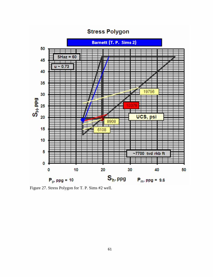
3. Stress estimation: Applying initializing information and premises to a Stress
Polygon at 7700 feet TVD (Figure 27), a stress state of SV = 19.4 ppg (7776 psi)
(53.6 MPa), SH = 19.1 ppg (7636 psi) (52.7 MPa), and Sh = 12.4 ppg (4964 psi)
(34.2 MPa) is obtained.
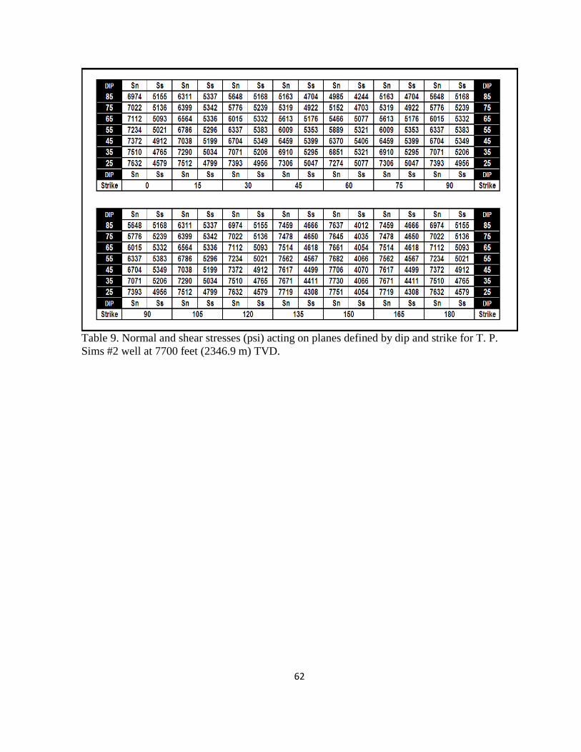
4. Evaluate reactivation:
a. Calculating normal stress (Sn) and shear stresses (Ss) (Table 9).
b. Calculating reactivation pressure (Pfr) (Table 10).
5. Combining reactivating pressure and normal stresses (Table 11).
Page 68
60
Figure 26. Dimpler measurements on the T. P. Sims #2 well. In the record above, dimples are
the small red dots generally located to the left of large red circles which enclose the posted
dimple diameter. The diameter of the dimples is measured with a surface magnifying glass
scaled in “ticks.” Field notes from Ruppel et al. (2008).
Page 69
61
Figure 27. Stress Polygon for T. P. Sims #2 well.
Page 70
62
Table 9. Normal and shear stresses (psi) acting on planes defined by dip and strike for T. P.
Sims #2 well at 7700 feet (2346.9 m) TVD.
Page 71
63
Table 10. For the conditions Sv = 7776 psi (53.6 MPa), SH = 7636 psi (52.7 MPa), and Sh =
4964 psi (34.2 MPa), the value within each cell (strike-dip combination) is the reactivation
pressure (Pfr in psi) calculated using a coefficient of sliding friction of 0.73 (lower most left
cell) and zero cohesion. Strike-dip combinations colored in yellow indicate that Pfr is less than
Sh, whereas the blue strike-dip combinations indicate that Pfr is above Sh. The gold colored cell
with red text is the lowest value presented.
Table 11. Results of taking the average of effective reactivation stress and the effective normal
stress derived from T.P. Sims #2 stress state.
Page 72
64
Fracture Summary
Table 12 is a summary of Tables 9, 10, and 11 for the reported natural fracture set in
the Barnett Shale that strike of 105° and dip of 74° (red ellipses). The estimated normal stress
is 6399 psi (44.1 MPa), the reactivation pressure is 4560 psi (31.4 MPa) and the average of the
effective reactivation pressure and the effective normal stresses is 1480 psi (10.2 MPa).
Discussion: Interactions of Hydraulic Fracture Treatment with Natural Fractures
Considering the T.P. Sims #2 stress situation and known natural fractures striking 105°
and dipping at approximately 75°, the estimated reactivation pressure is 4560 psi (31.4 MPa).
Such pressure is probably out of reach for most natural processes within the “oil field time
frame” (last few decades). However, this pressure is easily reached during hydraulic fracturing
operation (see Table 10, yellow colored cells), since the typical down-hole treating pressure is
equal to the sum of Sh (estimated at approximately 5000 psi or 34.5 MPa) and the net pressure
(net pressure approximately 1000 psi or 6.9 MPa; Lancaster et al., 1992). Such reactivation can
act to divert the fracturing fluids from the expected linear-elastic Mode I direction of 60° (SHaz)
to 105°. Since the orientation of the natural fracture is close to the yellow–blue transition on
Table 10, it can be easily imagined that a complicated “switching” back and forth between 60°
and 105° exists thereby creating a relatively wide corridor of a complex fracture network
compared to that of a linear-elastic Mode I fracture with a general orientation of approximately
60°.
Page 73
65
Table 12. For the reported natural fractures from the T. P. Sims #2 well with a strike of 105°
and a dip 74° (red ellipses) the estimated normal stress is 6399 psi (44.1 MPa) (a. Table 9), the
reactivation pressure is 4560 psi (31.4 MPa) (b. Table 10), and the average of the effective
reactivation pressure and the effective normal stresses is 1480 psi (10.2 MPa) (c. Table 11).
Page 74
66
CONCLUSIONS
1. Laboratory experiment and field observations indicate that fractures can be reactivated and
fail in shear. Such shear failure results in movement along the surface, subsequently
increases the ability of fluid to flow.
2. The method presented provides a means to quantitatively evaluate both shear and normal
stresses acting on a fracture.
3. The method presented provides a means to quantitatively evaluate the fracture reactivation
pressure.
4. Traditional “closure pressure” may or may not be equivalent in value to the minimum
horizontal stress (Sh).
5. The presented method provides insight into the interaction of hydraulic fracture treatments
with the reactivation of natural fractures in low permeability reservoirs.
Page 75
67
REFERENCES
Aguilera, R., 1980, Naturally Fractured Reservoirs. The Petroleum Publishing Company, 703
p.
Anderson, E.M., 1951, Dynamics of Faulting and Dike Formation With Application in Britain:
Oliver and Boyd, Edinburgh, 206 p.
Bandis, S.C., Lumsden, A.C., and Barton, N.R., 1983, Fundamentals of rock joint deformation:
Int. J. Rock Mech. Min. Sci. & Geomech., v. 20, no. 6, p. 249-268.
Barton, C.A., Zoback, M.D., and Moos, D., 1995, Fluid flow along potentially active faults in
crystalline rock: Geology, v. 23, p. 683-686.
Barton, N., Bandis, S.C., and Bakhtar, K., 1985, Strength, deformation and conductivity
coupling of rock joints: Int. J. Rock Mech. Min. Sci. & Geomech., v. 22, no. 3, p. 121-
140.
Byerlee, J.D., 1978, Friction of Rocks: Pure & Applied Geophysics, v. 116, p. 615-626.
Committee on Fracture Characterization and Fluid Flow, National Research Council, 1996,
Rock Fractures and Fluid Flow: Contemporary Understanding and Applications
Committee on Fracture Characterization and Fluid Flow, 586 p.
Couzens-Schultz, B.A. and Chan, A.W., 2010, An Alternative Leak-off Pressure Interpretation:
Journal of Structure Geology, v. 6, no. 13.
Page 76
68
Cumella, S.P., and Scheevel, J., 2008, The influence of stratigraphy and rock mechanics on
Mesaverde gas distribution, Pieance basin, Colorado: AAGP Hedberg Series, No. 3,
Understanding, exploring, and developing tight-gas sands, p. 137-155.
Eaton, B.A., 1969, Fracture gradient prediction and its application in oilfield operations:
Journal of Petroleum Technology, n. 246, p. 1353-1360.
Engelder, T., Geiser, P.A., and Alvarec, W., 1981, Role of pressure solution and dissolution in
geology: Penrose Conference Report, Geology, v. 9, p. 44-45.
Gale, J.F.W., Reed, R.M., and Holder, J., 2007, Natural fractures in the Barnett Shale and their
importance for hydraulic fracture treatments: AAPG Bulletin, v. 91 no. 4, p. 603-622.
Gidley, J.L., Holditch, S.A., Nierode, D.E., and Veatch, R.W., 1989, Recent advances in
hydraulic fracturing: Society of Petroleum Engineers, monograph v. 12, 452 p.
Goodman, R.E., 1989, Introduction to rock mechanics: John Wiley & son, New York, 220p.
Gretner, P.E., 1981, Pore pressure: Fundamentals, general ramifications, and implication for
structural geology (revised): AAPG Education Course Notes 4, 131p.
Gutierrez, M., Oino, L.E., and Nygard, R., 2000, Stress-dependent permeability of a de-
mineralised fracture in shale: Marine and Petroleum Geology v. 17, p. 895-907.
Halliburton, 1978, Halliburton Cementing Tables: Halliburton, Duncan, OK, 240 p.
Jaeger, J.C., and Cook, N.G., 1979, Fundamentals of rock mechanics, Chapman and Hall, New
York, 585 p.
Kent, W., 1899, Mechanical Engineer’s Pocket-Book: John Wiley & Sons, New York, 1119 p.
Kirsch, G., 1898, Die Theorie der Elastizität und die Bedürfnisse der Festigkeitslehre:
Zeitschrift des Vereines Deutscher Ingenieure, v. 42, p. 797-807.
Page 77
69
Lancaster, D.E., McKetta, S.F., Hill, R.E., Guidry, F.K., and Jochen, J.E., 1992, Reservoir
evaluation, completion techniques, and recent results from Barnett Shale development
in the Fort Worth Basin: SPE 24884.
Laubach, S.E., Olson, J.O., Gale, J.F.W., 2004, Are open fractures necessarily aligned with
maximum horizontal stress?: Earth and Planetary Science Letters, v. 222, p. 191-195.
Levorsen, A.I., 1967, Geology of Petroleum. W.H. Freeman and Company, San Francisco, 724
p.
Loucks, R.D., and Ruppel, S.J., 2007, Mississippian Barnett Shale: Lithofacies and
depositional setting of a deep-water shale-gas succession in the Fort Worth Basin,
Texas: AAPG Bulletin, v. 91 no. 4, p. 579-601.
Moos, D., 2007, Constraints on in situ stresses from strength of materials. SPE/AAPG/SEG
Workshop on Integrating Stresses and Pore Pressure Predictions for Exploration,
Drilling, and Production, Galveston, TX.
Moos, D. and Zoback, M.D., 1990, Utilization of observation of well bore failure to constrain
the orientation and magnitude of crustal stresses: application to continental deep sea
drilling project and ocean drilling program boreholes: J. Geophys. Res. v. 95, p. 9305-
9325.
Olsson, W.A., 1992, The effect of slip on the flow of fluids through a fracture. Geophysical
Research Letters, v. 19. no. 6, p.5 41-543
Ostensen, R.W., 1983, Microcracks Permeability in Tight Gas Sandstones: SPE Journal, v. 23,
no. 6, p. 919-927.
Page 78
70
Plumb, R.A. and Hickman, S.H., 1985, Stress-induced borehole elongation: A comparison
between the four-arm dipmeter and the borehole televiever in the Auburn geothermal
well: J. Geophys. Res. v. 90, p. 5513-5521.
Ramos, G.G., Chin, L.Y., Enderlin, M.B., 2008, Up-scaling of Rock Mechanical and
Petrophysical Properties from Grain Scale to Log Scale by Point-Stress and Wedge
Indentation Tests. 42nd U.S. Rock Mechanics Symposium, San Francisco, California.
U.S.A.
Ruppel, S.C., Loucks, R.G., and Gale, J.F.W., 2008, Barnett, Woodford, and Related
Mudrocks Succession in Texas Core and Outcrop: Bureau of Economic Geology,
Jackson School of Geosciences, University of Texas at Austin.
Schlumberger, 1972, Log interpretation: Volume I – Principles: Schlumberger Limited, New
York, 113 p.
Terzaghi, K., 1943, Theoretical soil mechanics: John Wiley, New York.
Tolman, C.F., 1937, Ground Water: McGraw-Hill, New York, 593 p.
Van der Pluijm, B.A., and Marshak, S., 2004, Earth Structure: an introduction to structural
geology and tectonics: W. W. Norton & Company, Inc., 656 p.
Warpinski, N.R. 2009, Integrating Microseismic Monitoring With Well completions Reservoir
Behavior, and Rock Mechanics: SPE 125239, SPE Tight Gas Completions Conference,
San Antonio, TX, 15-17 June 2009.
Weingarten, J.S. and Perkins, T.K., 1995, Prediction of sand production in gas wells: methods
and Gulf of Mexico case studies: SPE 24797.
Zoback, M.D., 2007, Reservoir Geomechanics: Cambridge University Press, 449 p.
Page 79
71
APPENDICES
Appendix 1: Flow data plots for each hour between hour 19 and 34.
Page 88
VITA
Personal Milton Bock Enderlin
Background Born June 21, 1945, San Angelo, TX
Son of George and Audrey Enderlin
Married to Victoria Travaglini, December 23, 1983
Education Bachelor of Science in Chemistry, 1977
Sonoma State University, Rohnert Park, CA
Bachelor of Science in Geology, 1977
Sonoma State University, Rohnert Park, CA
Master of Science in Geology, 2010
Texas Christian University, Fort Worth, TX
Experience Cryptographic System Specialist, 1966-1969
U.S. Air Force, Texas, Guam, Viet Nam
Intern Geologist, 1975-1976
California State Department of Water Resources, Rohnert Park, CA
Water Well Engineer’s Aide, 1976-1977
Sonoma County Water Agency, Rohnert Park, CA
Field Service Operations, 1977-1984: District Manager, General Field Engineer,
Regional Engineer, Dipmeter Specialist, Open hole Engineer,
Halliburton Logging Services
Development Program Coordinator, 1984-1987
Halliburton Logging Services, Fort Worth, TX
Manager Laboratory Petrophysics, 1987-1991
Halliburton Logging Services, Fort Worth, TX
Petrophysicist, 1991-2004
ConocoPhillips Petroleum Company, Bartlesville,OK
Structural Petrophysicist, 2004-2007
ConocoPhillips Petroleum Company, Houston, TX
Page 89
ABSTRACT
A METHOD FOR EVALUATING THE EFFECTS OF STRESSES AND ROCK STRENGTH
ON FLUID FLOW ALONG THE SURFACES OF MECHANICAL DISCONTINUITIES IN
LOW PERMEABILITY ROCKS
By Milton Bock Enderlin, M.S. 2010
Department of Geology
Texas Christian University
Dr. Helge Alsleben – Professor of Geology
Changing stress can affect the ability of fluid to flow along mechanical discontinuities
such as faults, fractures, or bedding planes. Stress can cause mechanical discontinuity to
reactivate in shear, resulting in an increase in fluid flow. The values for present-day horizontal
stress orientation and magnitude can be constrained from structural geology principles via
interpretation of mapped active features and wellbore information such as drilling history and
image logs. Stress magnitudes and orientation information is used to calculate the shear and
normal stress magnitudes acting on the mechanical discontinuities of all possible orientations.
Furthermore, the necessary magnitudes of fluid pressure within each mechanical discontinuity
that would be required to encourage shear failure reactivation are evaluated.
A laboratory experiment and an example from the Barnett Shale play are presented as an
application of the method. The Barnett example identifies likely orientations of pre-existing
fractures that could interact with fluids during hydraulic fracture stimulation.