Page 1
NASA Contractor Report 201601
z/ / .
A Method for Landing Gear Modelingand Simulation With ExperimentalValidation
James N. Daniels
George Washington UniversityJoint Institute for the Advancement of Hight Sdences
NASA Langley Research Center, Hampton, Virginia
Cooperative Agreement NCC1-208
June 1996
National Aeronautics and
Space Administration
Langley Research Center
Hampton, Virginia 23681-0001
https://ntrs.nasa.gov/search.jsp?R=19960049759 2018-06-03T14:36:40+00:00Z
Page 3
Abstract
An approach for modeling and simulating landing gear systems is presented.
Specifically, a nonlinear model of an A-6 Intruder Main Gear is developed, simulated,
and validated against static and dynamic test data. This model includes nonlinear effects
such as a polytropic gas law, velocity squared damping, a geometry governed model for
the discharge coefficients, stick-slip friction effects and a nonlinear tire spring and
damping model. An Adams-Moulton predictor corrector was used to integrate the
equations of motion until a discontinuity caused by a stick-slip friction model was
reached, at which point, a Runga-Kutta routine integrated past the discontinuity and
returned the problem solution back to the predictor corrector. Run times of this software
are around 2 minutes per 1 second of simulation under dynamic circumstances. To
validate the model, engineers at the Aircraft Landing Dynamics facilities at NASA
Langley Research Center installed one A-6 main gear on a drop carriage and used a
hydraulic shaker table to provide simulated runway inputs to the gear. Model parameters
were tuned to match one dynamic case. Other cases were then run with the updated
parameters and the results were in excellent agreement with the test data.
Page 5
Table of Contents
Abstract .................................................................................................................... i
Table of Contents .................................................................................................... iii
Nomenclature ........................................................................................................... v
List of Figures ....................................................................................................... viii
List of Tables ........................................................................................................... ix
Chapter 1: Introduction
1.1
1.2
1.3
1.4
1.5
Chapter 2:
2.1
2.2
2.3
2.4
Chapter 3:
3.1
3.2
3.3
3.4
3.5
Chapter 4:
4.1
4.2
4.3
Chapter 5:
5.1
5.2
Background ........................................................................................... 1
Objective ............................................................................................... 2
Literature Survey ................................................................................... 2
Research Significance ............................................................................ 5
Document Outline ................................................................................. 6
Problem Formulation
Initial Landing Gear Investigation ......................................................... 7
Nonlinear Model Development ............................................................. 9
Relation of Pressures to Stroke Position and Stroke Rate ................... 13
Summary ............................................................................................ 22
Numerical Analysis
Introduction ......................................................................................... 23
Model Integration ................................................................................ 23
Karnopp Friction Model ...................................................................... 26
Treatment of Discontinuities ............................................................... 28
Summary .. .......................................................................................... 29
Experimental Facility
Introduction ......................................................................................... 31
Test Equipment ................................................................................... 31
Summary ............................................................................................ 35
A-6 Experimental Parameter Determination
Introduction ......................................................................................... 36
Determination of Static Parameters ..................................................... 36
°°o
111
Page 6
5.3
5.4
5.5
Chapter 6:
Dynamic Testing ................................................................................. 45
Model Validation ................................................................................. 51
Summary ............................................................................................ 57
Conclusions
6.1 Conclusions .......................................................................................... 58
6.2 Future Research ................................................................................... 58
References .............................................................................................................. 60
Appendix A: Program Information and Listing
A.1 Program Set-Up ................................................................................. 63
A.2 Program Listing ................................................................................. 65
A.3 Sample Input Files ............................................................................. 83
A.4 Output Manipulation File ................................................................... 85
iv
Page 7
Nomenclature
As ........................ Genetic area for one snubber orifice (it2)
Cd ........................ Discharge coefficient of a flow through an orifice
Cas c ..................... Discharge coefficient of a snubber orifice during compression
Cas E ..................... Discharge coefficient of a snubber orifice during extension
Ct ......................... Tire damping coefficient 0bf*sec/ft)
C1/3 ...................... Redefinition of damping coefficient 0bf*seJ/it)
C_4 ...................... Redefinition of damping coefficient 0bf*sec2/ft)
Di, Ai ................... Diameter (ft) and area (ft a) of flow at point (i)
DL, A L.................. Diameter (ft) and area (ft a) of lower chamber
do, Ao ................... Variable diameter (it) and area (_) of main orifice
Dop ....................... Fixed diameter of orifice plate (It)
Dpi ....................... Diameter of piston shaft (f_)
Dpi_ ...................... Variable diameter of the metering pin (It)
DR, AR ................. Diameter (ft) and area (ita) ofrebotmd (or snubber) chamber
dsc, A_c ................ Diameter (it) and area (ita) of one snubber orifice during compression
_E, A E ................ Diameter (it) and area (ft 2) of one snubber orifice during extension
D., An .................. Diameter (ft) and area (fta) of upper chamber
El, E2, E3, E4 ........ Redefinition ofnonpressure terms in flow equations (ftS/(sec2*lbf))
f ........................... All friction in gear 0bf)
F i ......................... External force on body (i) (lbf)
Fow ....................... Variable friction due to moment created by offset wheel 0bf)
Fpeak ..................... Maximum sticking friction between two bodies 0bf)
F_ ......................... Relative force between bodies one and two 0bf)
fsc_ ....................... Constant friction due to seal tightness (lbf)
Fstick ..................... The force to stick the two bodies together (Ibf)
Ft ......................... Force transmitted through tire (lbf)
V
Page 8
g .......................... Gravitational acceleration (ft/sec 2)
Kt ......................... Tire stiffness (lbf/t_)
K1/3 ...................... Redefinition of spring stiffness term 0bf*ft _)
K2/4 ...................... Redefinition of spring stiffness term 0bf*ft'9
L .......................... Lift function on wing 0bf)
ma ........................ Moment arm of tire force acting on piston fit)
Mi ........................ Mass of body (i) (slug)
M L ....................... Piston Mass and Wheel/Tire Mass (slug)
Mo ....................... Moments about point O 0bf*ft)
M u ....................... Portion of Airplane Mass and Cylinder Mass (slug)
N ......................... Normal reactant force of cylinder wall on side of piston head 0bf)
P .......................... Pressure of a fluid at a point (psi)
Pi ......................... Pressure at point (i) in a fluid (psi)
PL ......................... Hydraulic pressure in lower chamber (psi)
Ps ......................... Hydraulic pressure in snubber chamber (psi)
Psi ........................ Pressure to which upper chamber is initially charged (psi)
Pu ......................... Pneumatic pressure in upper chamber (psi)
Q ......................... Volumetric flow rate of a fluid (t_/sec)
Qidea/ .................... Ideal flow through an orifice (ft-S/sec)
Qo ........................ Flow through the main orifice (fia/sec)
Qreal ..................... Real flow through an orifice (flZ/sec)
Qsc ....................... Flow through a snubber orifice during compression (ftZ/sec)
Qs E....................... Flow through a snubber orifice during extension (f_/sec)
stp ....................... Minimum separation between bearings when fully extended (ft)
U, U ................... Input position (ft) and velocity (ft/sec) from ground
V .......................... Velocity of a fluid at a point (ft/sec)
Vi ......................... Velocity at point (i) in a fluid (ft/sec)
V i......................... Velocity of body (i) (ft/sec)
vi
Page 9
Vr.........................Relativevelocity (ft/sec)betweenbodiesoneandtwo
1;'........................Timederivativeof relativevelocity(ft/sec2)
Wi........................Momentumof body (i) (slug*ft/sec)
........................Time derivativeof momentumof body(i) (lbf)
X,, ,_'o, X, .......... Wheel axle position (t_), velocity (ft/sec), and acceleration (ft/sec 2)
X_ ........................ Stroke remaining in strut (ft)
X, ........................ Stroking rate (it/sec)
X_i........................ Stroke position at which upper chamber is charged (ft)
X_,, .................... Fully extended stroke value (it)
Xwg, _'wt, X'_s ..... Wing/Gear position (it), velocity (it/see), and acceleration (ff/sec 2)
Z .......................... Height of a point in a fluid from some reference (it)
Zi ......................... Height at point (i) in a fluid fit)
1/3 ....................... Subscripts associated with compression
2/4 ....................... Subscripts associated with extension
Greek Symbols
13.......................... The ratio of orifice area over flow from area (ff/ft)
5 .......................... Velocity deadband near zero (ft/sec)
T .......................... Polytropic gas constant
_t .......................... Coefficient of friction between piston head and cylinder wall
v .......................... Specific weight of a fluid (slug/(it*sec2))
p .......................... Density of a fluid (slug/ft 3)
vii
Page 10
List of Figures
Figure 2-1:
Figure 2-2:
Figure 2-3:
Figure 2-4:
Figure 2-5:
Figure 2-6:
Figure 2-7:
Figure 3-1:
Figure 4-1:
Figure 4-2:
Figure 5-1:
Figure 5-2:
Figure 5-3:
Figure 5-4:
Figure 5-5:
Figure 5-6:
Figure 5-7:
Figure 5-8a:
Figure 5-8b:
Figure 5-8c:
Figure 5-8d:
Figure 5-9a:
Figure 5-9b:
Schematic of typical telescoping landing gear ...................................... 7
Schematic of a telescoping main landing gear ..................................... 11
Schematic of upper mass and main cylinder ...................................... 12
Schematic of lower mass .................................................................... 13
Control volume between piston and orifice plate .............................. 16
Control volume for the snubber chamber .......................................... 18
Schematic of gear for friction model development ............................. 21
Simple two mass system with slip stick friction .............................. 26
Schematic of experimental set up ...................................................... 32
Instrumented A-6 landing gear ........................................................... 34
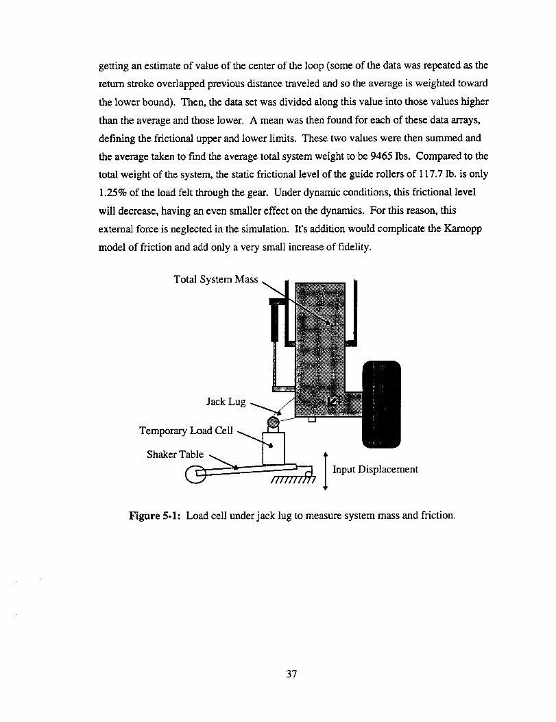
Load cell under jack lug to measure system mass and friction .......... 37
Total weight of the system and frictional hysteresis loop ................ 38
Weight of lower mass and frictional hysteresis loop ......................... 39
Experimental tire load-deflection curve ............................................. 40
Pressure-stroke curve and fitted analytical expression ...................... 42
Result of "pressure load" subtracted from axle load measurements.. 43
Zero centered frictional load data ...................................................... 44
Frequency response comparison of strut stroke to shaker input ..... 48
Frequency response comparison of upper mass position to
shaker input ...................................................................................... 49
Frequency response comparison of upper chamber pressure to
shaker input ...................................................................................... 50
Frequency response comparison of upper chamber pressure to
shaker input ...................................................................................... 50
Frequency response comparison of strut stroke to shaker input ..... 51
Frequency response comparison of upper mass position to
ooo
vul
Page 11
shaker input ...................................................................................... 52
Figure 5-9c: Frequency response comparison of upper chamber pressure to
shaker input ...................................................................................... 52
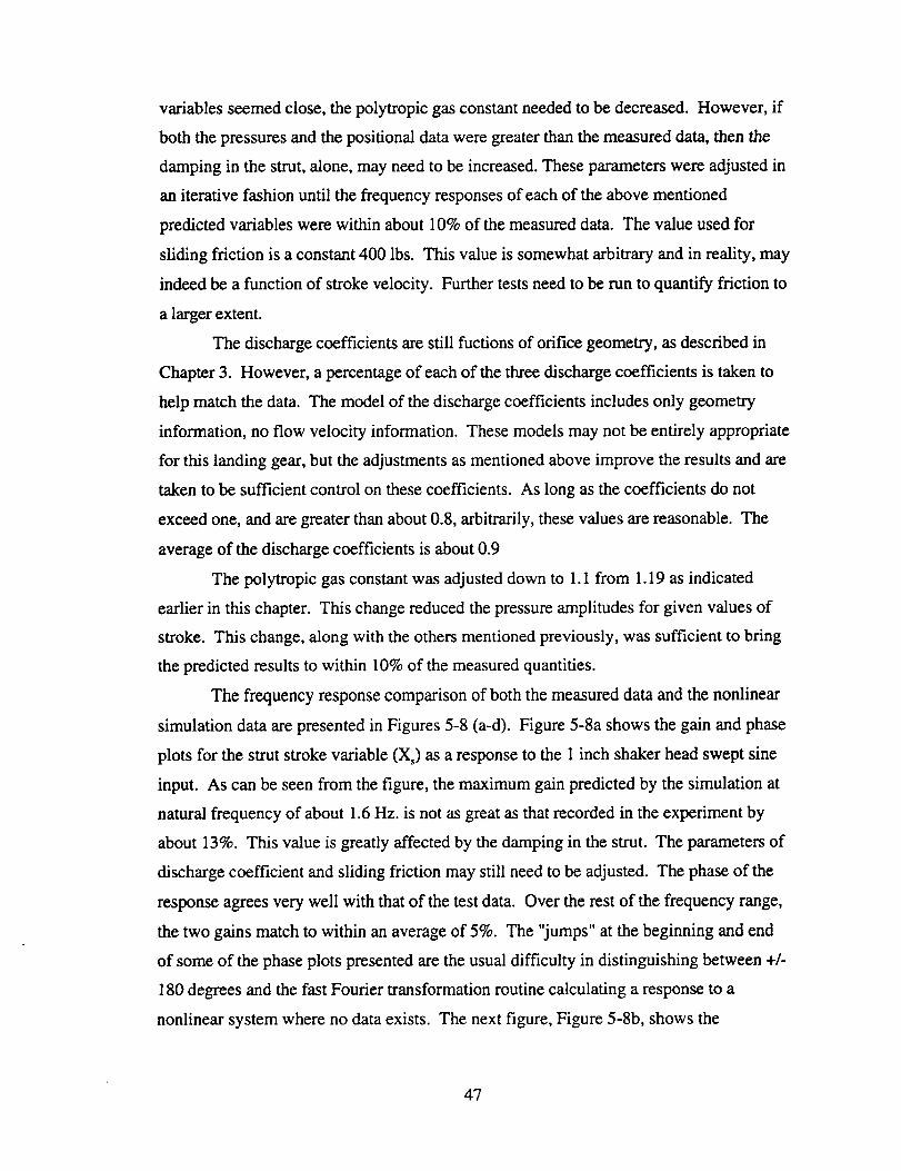
Figure 5-9d: Frequency response comparison of upper chamber pressure to
shaker input ...................................................................................... 53
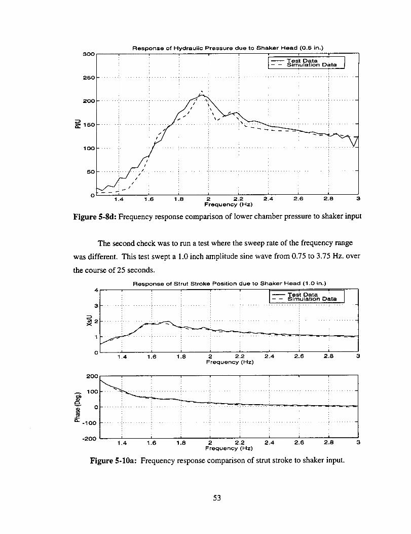
Figure 5-10a: Frequency response comparison of strut stroke to shaker input... 53
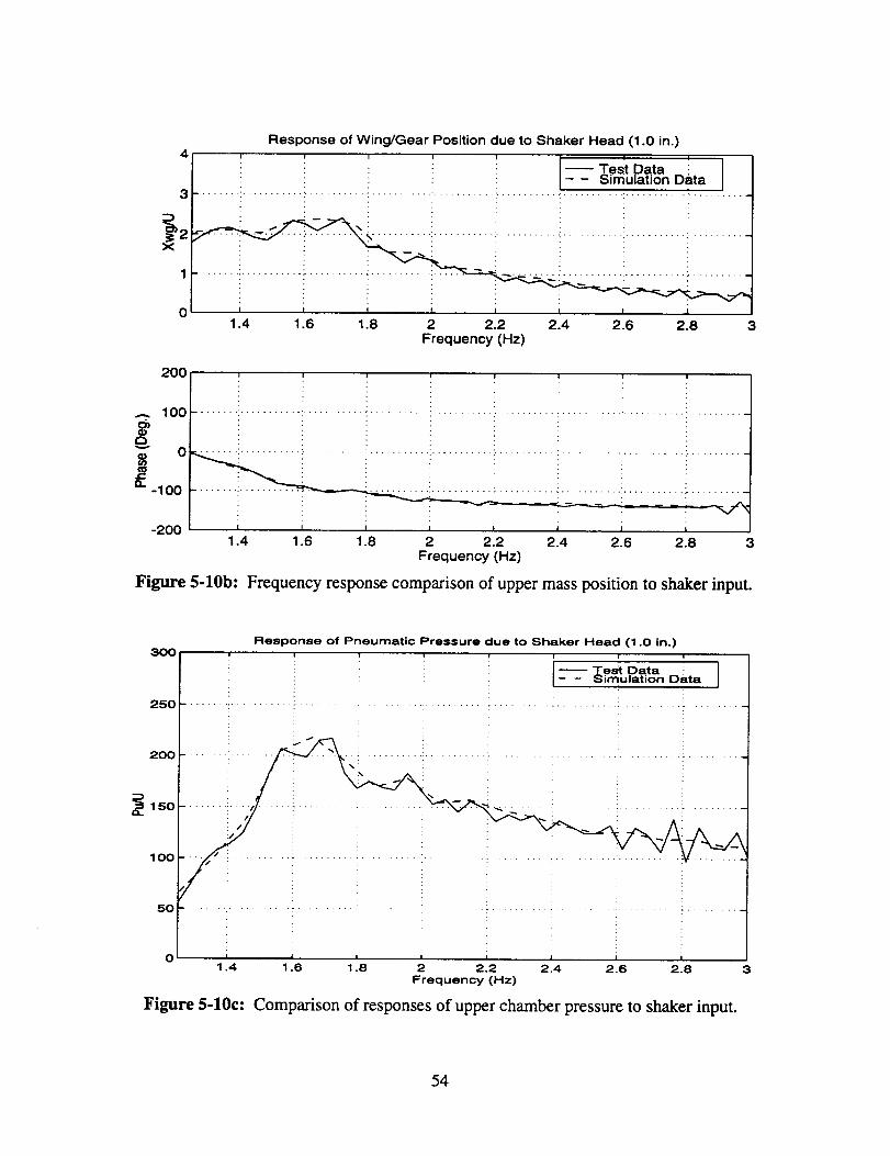
Figure 5-10b: Frequency response comparison of upper mass position to shaker
input ................................................................................................ 54
Figure 5-10c: Comparison of responses of upper chamber pressure to shaker
input ................................................................................................ 54
Figure 5-10d: Comparison of responses of lower champer pressure to shaker
input ............................................................................................... 55
Figure 5-1 la: Time history of strut position as gear encounters a step bump ..... 56
Figure 5-1 lb: Time history of Wing/Gear Position as gear encounters a step
bump .............................................................................................. 56
List of Tables
Table 4-1: Instrument guide on A-6 test specimen ............................................... 34
ix
Page 13
Chapter 1: Introduction
1.1 Background
In recent years, NASA and many aerospace companies have increased their
research focus on the High Speed Civil Transport (HSCT). The concept is to fly a
supersonic (mach 2.4) airplane to various places on the globe at an economical price for
both carrier and passenger use. Its overall appearance will be similar to that of the
Concorde, a current, expensive supersonic carder.
To make the HSCT more cost effective, much effort is being expended in the
design stage. One major problem encountered in its development is the trade-off between
structural rigidity and total weight. To this point, the structure of the fuselage and wings
has been designed for aerodynamic performance. In the early stages of design, however,
landing gear location and dynamic performance are rarely considered. Since the fuselage
on the HSCT is very long and slender, it is very sensitive to external, low frequency
disturbances, or vibrations. Therefore, a goal of the landing gear design is to reduce
disturbance transmission from the ground to the fuselage.
Computer simulations are being developed to study this disturbance transmission
problem. The task is to take information concerning gear dynamics, fuselage dynamics,
runway profile, and taxi speed, to develop a simulator for predicting aircraft ground
response. Simulation of landing gear dynamics has been the subject of much research for
many years. The military has long been interested in simulating gear response to
repaired, bomb-damaged runways. A great deal of effort has been applied to the problem
of determining how well to repair a runway to prevent landing gear failures. This effort
did not focus on changing the gear (i.e. to control the force transmission), but rather on
changing the runway repair specifications. Active control concepts may render landing
gears less sensitive to rough runways, decreasing the time needed to repair damaged
runways, and thus allowing quicker response of military missions.
Page 14
1.2 Objective
This document will present an approach for modeling and simulating landing gear
systems. Specifically, a nonlinear model of an A-6 Intruder Main Gear is developed,
simulated, and validated against test data. This model includes nonlinear effects such as a
polytropic gas model, velocity squared damping, a geometry governed model for the
discharge coefficients, stick-slip friction effects and a nonlinear tire spring and damping
model. To validate the model, engineers at the Aircraft Landing Dynamics Facility at
NASA Langley Research Center installed one A-6 main gear on a drop carriage and used
a hydraulic shaker table to provide simulated runway inputs to the gear. Model validation
used both quasi-static and dynamic tests. In summary, then, this research presents a
comprehensive mathematical formulation of landing gear systems, verifies the modeling
techniques with tests, and discusses approaches for further model correlation using the
test results.
1.3 Literature Survey
Concurrent and past work of this kind have been generally to predict taxi loads of
military aircraft over repaired, bomb-damaged runways. This work has led to extensive
modeling of military aircraft with the goal of determining minimum repair procedures to
runways to prevent gear failure on rollout. One major accomplishment of this research is
the HAVE BOUNCE _ simulation program. Using this program, the USAF has
simulated the dynamic response of many military aircraft over bomb damaged runways.
These simulations are validated with test data and are used to identify component
weaknesses and operational limits. Validation of these simulations is usually achieved
through the use of the Aircraft Ground Induced Loads Excitation (AGILE) 2 test facility at
Wright-Patterson Air Force Base. Simulations usually combine nonlinear coupled
differential equations of the landing gear with linear techniques describing the fuselage
structure to generate the total aircraft response. Each of these simulations is usually very
good, but each is also very tailored for the plane in question. In addition, the military is
concerned mainly with the problem of traversing repaired sections sequentially on a
runway. They have, therefore, limited the inputs to their models mainly to the various
classes of repairs.
2
Page 15
Another approach discussed in the literature uses data from tests to determine
parameters of a state space model for the landing gear and fuselage 3. These parameters
are included in a quasi-linear formulation through look-up tables. Depending on the exact
form of the model and the measurement capability, the results of this type of formulation
are fair to good in comparison to actual test data. This approach is good when test data is
easily accessible for parameter determination, and simulation computation time is limited.
Freymann 4 revisited an experiment by Ross and Edson 5 in which an actively controlled
servovalve is connected to a landing gear to augment damping in the system. Ross and
Edson 5 described an electronic controller and an actively controlled landing gear which
was found to significantly reduce forces sustained by an aircraft during takeoff, landing
impact and rollout. The results were obtained analytically through the use of a linearized
model of the equations of motion and confirmed experimentally. The servo-controller
was designed to maintain a certain command force level by porting flow into and out of
the landing gear. This approach to active control, however, is very expensive in terms of
weight and complexity. There, also, was no recourse developed in case of servo failure.
Their model included a linear tire spring, no tire damping, no metering pin and no
rebound chamber. However, they did include friction and velocity squared fluid
damping. Freymann extended this research by implementing this active control scheme
on a fighter aircraft and testing this aircraft's response to various frequency inputs. The
control system performed well in attenuating aircraft motions.
Much effort has been exerted by Stirling Dynamics 6"7in the field of simulation
and control. Their main simulation program includes many highly detailed models of the
various components of several types of landing gear. The program allows part selection
for individual gear types and outputs landing gear dynamic responses in terms of
positions, velocities, accelerations and angular equivalents for any pan of the gear or
fuselage which is selected as a node. Other outputs were subsystem force interactions.
Extensive validation has proven this to be a very accurate simulation tool. The complexity
of the model generally captured most dynamic effects seen in test data. This same
program was used to test an active orifice concept applied to the nose gear of a typical
transport plane. These results showed reduction of peak and root mean square values of
normal acceleration, especially in the nose and tail section of the plane. An active orifice
mechanism was not detailed, only an assumed behavior. This is a very good program for
Page 16
landinggeardesignandtestingof existinggearconfigurations.However,asimpler
model wouldallow thephysicsof thestrut,only, to bescrutinized,leadingperhapsto a
clearerunderstandingof landinggearbehavior.
Researchinto thebehaviorof asupersoniccarrierduringgroundoperationswas
performedby C.G. Mitchells. His theoreticalanalysisandtestexperiencewith the
Concordehasshownthatthesupersonictransportis moresensitiveto unevenrunways
thanthesubsonictransport.Resultsreportedin [8] show that much care must be taken to
minimize undercarriage stiffness and friction if problems of cockpit vibrations and
airframe and undercarriage fatigue were to be avoided.
Ramamoorthy 9 performed a parameter study on his model of an articulated
landing gear and found that changes in the discharge coefficient could alter the results
dramatically. No quantitative conclusions were made and no validation of the model was
performed. However, Wahl j° found that the coefficient can alter forces transmitted to the
fuselage by as much as 25% and that proper estimation of this parameter needs to be
based on both the Reynolds number and orifice geometry. A semi-empirical model
developed by Bell, Schlichting, Knudsen et. al. was used for this parameter. With this
model for the discharge coefficient, Wahi _°developed a landing gear model with two
degrees of freedom to investigate the optimization of the metering pin shape. The results
of this model compared well to flight and drop tests. Optimization of the metering pin,
for this particular case, showed some improvement in the force reduction. Once a
metering pin shape has been defined, it cannot change. An active orifice concept would
allow the damping characteristics of the gear to be continuously changed in reaction to
any input to reduce vibration transmission.
An optimization of many strut characteristics was performed by Li, Gou-zhu, and
Qing-zhi 1]. This paper described an optimization approach for landing gear design using
as design variables the initial pressure, initial air volume, and an artificial oil damping
coefficient (which in reality, is a function of the hydraulic and pneumatic areas as well as
the discharge coefficient and oil density). The objective function was the mean square
value of the fatigue power spectral density. Constraints were in the form of landing
impact energy, static compression ratio, maximum compression ratio and limits on the
damping coefficient. The results show a significant reduction in the accumulated fatigue
on the simulated Boeing 707. What the results fail to show, however, is whether the
4
Page 17
upperandlower limits onthedampingcoefficientsarephysicallyachievable.Thelimits
did not includeconsiderationsof geometryandrealisticdischargecoefficientvalues.
Doyle_2providesanexcellentliteraturesurveyonaircraftgrounddynamic
simulationtechniques.His reportcontainsa brief summaryof thecomputerprograms
written topredictthedynamicdisplacementsandforcesresultingfrom nonflightaircraft
operations.Thecapabilitiesof eachprogramandtheirlimitationsandnumerical
techniquesarecited.
1.4 ResearchSignificance
Thesignificanceof thematerialtreatedin thisresearchis thatit bringstogetherin
oneplaceacomprehensivedevelopmentof thetheoryof telescopinggear.This
documentcontainsthedevelopmentof theequationsof motionanddetailsthemore
standardpracticesof expressingthemin termsof physicallymeasurablequantities.The
modelhasonly two degreesof freedom,bothin theverticaldirection. In the investigation
of loadstransmittedinto thefuselage,though,this is themostimportantdirection. The
modelis fully nonlinearandincludessucheffectsasapolytropicgasmodel,avelocity
squareddampingterm,which includesa dischargecoefficientthatis afunctionof orifice
geometry,extensiondamping,stick-slipfriction in thegear,andnonlineartire model. All
parameterssuchaspolytropicgasconstant,orificegeometry,frictional quantities,etc.
appearexplicitly in theequations,andcanbeusedin asensitivityanalysis.Also,
optimizationof geargeometryandinitial chargepressuresandvolumesis easily
accomplishedusingthis model. In theend,controlconceptscanbe linkedto thismodel
for investigationof forcetransmissionreduction.
Thisresearchalsotreatsthesubjectof numericalintegrationof theequationsof
motion. Thestiff, nonlinear,anddiscontinuousbehaviorof theseequationsmakethisa
difficult problemto solvenumerically,andmanyconsiderationsweremadeto makeit
easier.Also, thisdocumentdetailsa seriesof testsandproceduresby whichto validate
themodel. Thisvalidationis bothstaticanddynamic. A frequencyresponsemethod
wasusedto updatetheparametersin themodelandothertypesof casesto validatethe
simulation.
Page 18
1.5 Document Outline
This document is divided into six chapters. After the introduction in Chapter 1,
Chapter 2, discusses the theoretical and mathematical development of the equations of
motion of a landing gear. Chapter 3 details the method in which these equations were
numerically implemented and some of the problems that were encountered. Chapter 4
discusses the equipment used in the experimental validation effort. The next chapter
describes the test procedures that were implemented to validate this simulation and some
statements about error control. Finally, Chapter 6 will discuss some future research and
experimental plans and presents some concluding remarks. Also included, in Appendix
A, is the FORTRAN program used to obtain the simulation results shown in this
document.
6
Page 19
Chapter 2: Problem Formulation
2.1 Initial Landing Gear Investigation
This chapter is intended to familiarize the reader with landing gear terminology
and to demonstrate a mathematical development of the equations of motion for a
telescoping landing gear. Figure 2-1 is intended to acquaint the reader with basic landing
gear components. It shows the simplified components of a telescoping, main landing
gear (as opposed to a nose gear).
1) Upper Mass (Fuselage)
2) Nitrogen Gas (Pneumatic Spring)
3) Outer Cylinder
4) Hydraulic Fluid
5) Orifice Plate
6) Metering Pin
7) Snubber Orifice
8) Snubber (Rebound) Chamber
9) Lower Piston
10) Tire
Figure 2-1: Schematic of typical telescoping main landing gear.
Page 20
Point1on thefigureis arigid bodyrepresentationof theaircraftfuselagethatthe
gearcarriesandis the interfacebetweentheplaneandthegear.Point2 is achamber
containingcompressednitrogenwhichservesasaspringthatcarriestheweightof the
planein groundoperations.Point3 refersto themain,uppercylinderwhichhousesthe
compressedgas,hydraulicfluid, andwithin whichthepistonslides.Thehydraulicfluid
is representedby theshadedarealocatedby point4. Point5 is theorificeplate. It is
essentiallyacircularplatewith aholein thecenterthroughwhichthehydraulicfluid
flowswhenthestrut is stroking. It, alongwith themeteringpin,point 6, controlsthe
dampingcharacteristicsof thegear.Themeteringpin is rigidly fixed to thepistonhead.
As the strut strokes, the changing size of the metering pin passes through the constant
hole in the orifice plate, causing a variable effective orifice diameter, i.e. variable fluid
damping. Nose gear on most planes have no metering pin. Point 7 locates one of many
rebound or snubber orifices (usually around 12, depending on the gear). These holes lead
into a small volume on the backside of the piston head (point 8) called the rebound or
snubber chamber. The purpose of the snubber is to provide damping when the strut
extends. The snubber orifices are variable in that they are dependent upon a slip ring that
either allows a large orifice in the compression stage or a smaller orifice in the extension
stage. Point 9 is the piston. It houses the metering pin and is also the rigid connection of
the wheel axle. Finally, point 10 is the tire. This element of the gear adds both spring and
damping characteristics to the overall performance of the gear, and is selected carefully
for various applications.
A study by Ross and Edson 5 of Hydraulic Research provided the initial
information for this research. They developed nonlinear equations for a simplified
telescoping landing gear. They then linearized the equations about the ground equilibrium
point and studied the effect of an active damping control scheme. The model they
developed did not include a metering pin or a rebound chamber. However, their model
included a servovalve to port fluid from one chamber (upper or lower) to the other to
control the gear damping response, precluding the usefulness of the snubber or metering
pin. This method of control requires high hydraulic pressures and large pumps and
plumbing to accomplish the task, making it difficult to implement. The report, however,
did conclude that active control gear can reduce the ground loads transmitted to the
fuselage. Their simulation was validated using experimental equipment and facilities of
8
Page 21
HydraulicResearch.Thelinearizedmodeldid not allowexplicit investigationof orifice
diametersandotherparameterscriticalin understandingthelandinggear'sdynamic
behavior.But, thesestudieswereconsideredinvestigativein natureandledto amore
completeunderstandingof someof thecomplexdynamicsof landinggear.
2.2 Nonlinear Model Development
To extend the work by Ross and Edson 5, this research discusses an independent
development of a mathematical model of a main landing gear with all the relevant
physical parameters included. The nonlinear equations of motion are developed for a
telescoping main gear. The analytical model used is a representation of an A-6 Intruder
main gear. This gear was chosen because facilities exist to test and characterize an A-6
gear for simulation validation. Specific details of the gear were taken from the technical
drawings supplied by the Grumman Company.
An initial model was developed that only included the air-spring above the fluid,
fluid dynamics through a fixed orifice, and a linear tire spring term. This simple model
allowed some trend comparison between the results of this model and the early results of
the linearized gear of Edson and Ross 5. A metering pin was then added to change the
main orifice effective diameter as a function of stroke. Another variation from Edson and
Ross was the addition of a snubber, or rebound chamber. This feature provides damping
while the gear is extending. Since this new model is to be validated with test data, some
attempt to quantify frictional effects was also made. The model includes constant seal
friction as well as a variable friction that is a function of stroke. In a further effort to be
realistic, a nonlinear tire model was added. This tire model has a spring rate that is a
function of tire deflection and damping proportional to compression rate. In the equations
developed below, the spring and damping coefficient are used as if they were constant.
The nonlinear characteristics of each of these terms is included in the equations of motion
that axe actually integrated.
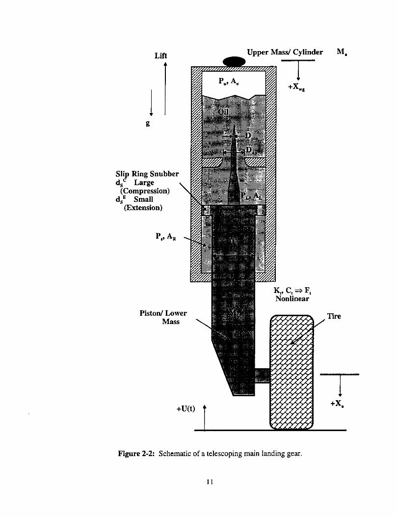
Figure 2-2 is a schematic of the gear used in the development of the equations of
motion. This schematic is representative of a general telescoping-type main landing gear.
It includes the aerodynamic lift on the plane, Lift, the upper mass (of the plane's fuselage)
and the mass of the main cylinder lumped together as a rigid mass, M_ and the mass of
the piston and the mass of the tire, also lumped together as M E. The inertial coordinate of
9
Page 22
theuppermassisXws.The zerovaluefor Xwsis whenthegearis fully extendedwith the
tire just touchingtheground. Fromthissamegearconfiguration,Xa,thecoordinateof
thelower mass,is takenaszeroattheaxleof thetire. Therefore,whenthegearis in
somecompressedstate,X, measuresthedeflectionof thetire whenthegroundinput,
U(t), iszero. In thecompressednitrogenchamber(uppercylinder)with crosssectional
areaof A_, the pressure is P.. Likewise, in the lower chamber with cross sectional area of
At., there is a pressure of Pt.. In the snubber chamber, with annulus area of A e, the
pressure is defined to be P.¢ The orifice plate has a hole of diameter D_, through which
the metering pin, with variable diameter Dpin moves. Fluid reaches the snubber chamber
through the orifices ds c and ds E, where the superscripts represent either the compression
mode or extension mode respectively. The diameter of the piston, Dpi, is used to calculate
A_. Simply subtract the area of the piston shaft from that of the lower cylinder to get A R.
The tire is also shown in Figure 2-2 with a distinction of pointing out that the tire spring
and damping coefficients, I_, and C t are nonlinear and contribute to the calculation of the
tire force F t.
10
Page 23
Li_ Upper Mass/Cylinder M_,
Slip Ring Snubber
ds c Large
(Compression)
ds E Small(Extension)
Ps, AR
Piston/Lower
Mass
Kt, Ct =_ F tNonlinear
The
+U(t)
Figure 2-2: Schematic of a telescoping main landing gear.
11
Page 24
Lift
TTTTTTP., A_
L!olyLiTT'r TTT
PL, AL
ARi PistOnDpi
I
_ ML
I
P_ _
I
+X_g
Figure 2-3: Schematic of upper mass and main cylinder
Figure 2-3 shows the forces acting on the upper mass. Balancing the forces on the upper
mass gives the following equation:
M.X_s = Mug- L- P_Ao - PL(AL -- ,4o)+ P_AR T f (2.1)
The term on the left hand side of Eq. (2.1) is the inertial motion term, g is the gravitational
acceleration, f is the friction present in the gear, and all other terms are as described
previously. This equation assumes that the fluid pressure in the upper cylinder is identical
to the pneumatic pressure. In this development, the variable Ao, the main orifice area,
reflects the fact that the metering pin is included, i.e. it is a variable cross-sectional area
depending on stroke.
12
Page 25
f kv
I
I" .......... =1
"A"........ _ 0 _ ........
I I
I I
r] Piston
I,
MLg F,
r .......... "I
I
!SAs
r" iI
Ps
I
I
I I
k )v
+ X a
Figure 2-4: Schematic of lower mass.
Figure 2-4 shows the forces acting on the piston. Summing the forces on the lower mass
(piston) the force balance equation is:
MeX . = Meg+ PL(AL-As)-_(AR-As)-Ft 4- f (2.2)
where the left hand side of Eq. (2.2) is the inertial motion of the lower mass and A Sis the
area of the snubber orifice. F, is the force that is transmitted through the tire from the
ground and has the form:
v,=x,(x,.+v)+C,(Xo+O)where the tire force is a function of a nonlinear tire stiffness and a damping force that is
composed of a damping coefficient that is proportional to the tire stiffness and the time rate
of change of the tire deflection.
2.3 Relation of Pressures to Stroke Position and Stroke Rate
The pressure terms in Eqs. (2.1) and (2.2) are as yet unknown and need to be
related to the positional variables Xws and X_ or their derivatives. The pressure of the
compressed nitrogen in the upper cylinder can be described by the polytropic gas law for a
closed system as:
13
Page 26
tx...-x:)(2.3)
where X, is the stroke available, given by:
X, =Xw,- X a (2.4)
with X_ as some initial length, P,j, the charge pressure at X,,, and 7, the polytropic gas
constant. X,,,_, is the maximum value to which the gear can be extended. This form of
representation of the pressure change is assumed to happen as a quasi-equilibrium
process 13. The significance of the polytropic gas constant is that it describes the type of
process that occurs. For example, if),= 0, the process would be isobaric, or constant
pressure. However, for an ideal gas, 7" 1, corresponding to an isothermal (constant-
temperature) process. If), is equal to the ratio of the specific heats of a gas, the process is
isentropic, or constant entropy. These cases are idealizations of particular processes. In real
situations though, the polytropic gas constant is not constant at all and is usually calculated
from pressure-stroke data. An average value is usually sufficient in application.
Equation (2.3) was defined in such a manner that P, will become very large when
X, is near Xm.,, i.e. the gear is nearly completely collapsed. This is a suitable
representation of the process, with only the polytropic gas constant 7 as an unknown.
The pressures (PL and P,) of the fluid in the lower cylinder and in the snubber are
related to the flow rates of the fluid into and out of those regions. The volumetric flow
rates through the orifice plate hole, Qo, and the snubber orifices, Qs, can be determined by
combining the continuity equation and Bemoulli's equation for fluids '4. Flow is always
from the higher pressure to the lower pressure. Bernoulli's equation for an incompressible
fluid states that along a streamline 'a,
P/a) + (1/2g)V 2 + Z = Constant (2.5)
where P is the pressure at some point, g is the gravitational acceleration, V is the velocity of
the flow, a) is the specific weight of the fluid which is equal to the fluid density (p)
multiplied by the gravitational acceleration (g), and Z is the height difference from some
zero reference. This equation assumes that the viscous effects within the fluid are
negligible, the flow to be steady and incompressible, and that the equation is applicable
along a streamline.
Equating Bemoulli's equation (Eq. (2.5)) at two points in the flow along the same
streamline yields:
14
Page 27
P1/19+ (1/2g)Vl2+ Z I = PJ_ + (1/2g)V2 2 + 7-,2 (2.6)
In the case of a landing gear, the potential distance between Z 1and 7_,2 can be neglected as
the distances involved are very small compared to the other terms. Equation (2.6) with the
continuity equation for incompressible fluids which states Q = AjV 1 = A2V 2 allows for the
solution of this equation in terms of one of the velocities. Assuming that P_ > P2, i.e. the
flow is from Pt to P2, then solve for V1 from the continuity equation as:
and substitute this velocity into Eq. (2.6) and solve for V2:
V2 = + .... _ (2.7)
When the flow reverses, i.e. P_ < P2, then the velocity at point 2 is described by the above
equation with the pressure terms switched and a negative sign on the square root. The ideal
volumetric flowrate (Q_t) for an incompressible fluid can be expressed as Q_ = A*V.
In a realistic flow situation though, there is a loss due to the Vena Contracta effect. This
loss is empirically quantified by a discharge coefficient (Ca), which represents the
percentage of the ideal flow that actually occurs. This coefficient, when multiplied by the
ideal flow, yields Q_l as:
Qre._l= CaQi_leal = ACdV (2.8)
Substituting Eq. (2.7) into Eq. (2.8) for velocity:
l/2Q"'t=ACd (D___kl41
P 1-_,D2 ) )
"-* > (2.9)
For the landing gear shown in Fig. 2-2, there are two flows that are of concern, the flow
through the orifice plate and the flow into and out of the snubber chamber. Define Qs c as
the flow rate into the snubber chamber in the compression mode, where the snubber orifice
area (A s) becomes As c, which allows larger flow. The flow rate through the snubber
orifice during the extension mode is defined as Qs E , and the area A s becomes As E, which
15
Page 28
only allowssmall,restrictedflow. In bothcases,theflow throughthemainorifice plateis
Qo.
r Qo, Pu
Q: PL,AL QEII
j--_ Piston --_ J T+X_-JQs c "Dpi Qs c --
p, _ p, ,AR
Figure 2-5: Control volume between piston and orifice plate.
Figure 2-5 shows the direction of fluid flow into and out of a control volume in the lower
chamber as a function of stroke mode (extension or compression). In relating the flow
rates to the pressures, defining a control volume as shown by the dashed line in Figure 2-5
is necessary. The stroke rate is defined as:
.,_, = _'.s - ,_'_ (2.10)
where the compression mode is given by ,_ > 0.0, and the extension mode by ,_', < 0.0.
The flow is assumed to be negative leaving the control volume, and is positive entering it.
For an incompressible fluid, the volumetric flow rates for compression and extension can
be written as:
Q,, + QC + AL.,_,. =0.0 (2.11)
during the compression mode, and:
Qo+ Qff + ALL = 0.0 (2.12)
during the extension mode. Equation (2.9) defined the general form of the equation for a
flow rate. Substituting the appropriate pressures, areas, and diameters into Eq. (2.9), the
flow rate through the orifice plate during the compression mode (when flow is out of the
control volume and PL > Pu and P,) can be written as:
16
Page 29
-AoC.I . 2- forP6 > _ (2.13)
where do is the effective diameter of the main orifice, D L is the diameter of the lower
chamber, and C a is the discharge coefficient of the main orifice. The flow through the
snubber orifices during this mode is described by:
QC = _AcC c /.( 2 p,for PL > P_ (2.14)
with ds c as the diameter of a snubber orifice, Dr. as described above, Cas c is the discharge
coefficient of the snubber orifice and As c is the effective area of the snubber orifice.
Similarly, for the extension mode, where flow is into the control volume (PL < Pu and Ps):
iI PQo=AoCa 7" .,'_-P_ forP. > PL (2.15)
p 1 _D,_) )
where the difference between this equation and Eq. (2.13) is that the pressure terms have
exchanged positions and the whole term is now positive. The flow rate through the
snubber orifices during the extension mode is given by:
II 2OJ=A C , -pL for P_ > PL (2.16)
where D R is the effective diameter of the annulus snubber chamber, ds E is the diameter of a
snubber orifice, As E is the effective area of the snubber orifices and Cas E is the discharge
coefficient of the snubber orifices in the extension mode. To simplify Eqs. (2.13), (2.14),
(2.15), and (2.16), let the non-pressure terms be redefined as:
17
Page 30
i>/l4 '
/Pl- _:)e_ =E,,
respectively. Substituting Eqs. (2.13) and (2.14) into Eq. (2.11) and Eqs. (2.15) and
(2.16) into Eq. (2.12) using this new notation, rewrite Eqs. (2.11) and (2.12) as:
-E_f-_L-P_-E2_L-P _ + AL,_', = 0.0
E._,qr-_ - PL +E4_-P L +At,_, = 0.0
for X, > 0.0
for X_ < 0.0
(2.1 la)
(2.12a)
"t" -I --
IdOlS C
ds
AR, P_, DR
t. ........
/N
¢/ Cylinder Wall
Figure 2-6: Control volume for the snubber chamber.
Additional information about the flow rate-pressure relationship can be gained by
studying a control volume in the snubber chamber as shown by the dashed line in Figure
2-6. The variables A Rand D Rin Fig. 2-6 are the rebound chamber annulus area and
18
Page 31
effectivediameterrespectively.Psis thepressurein thereboundchamberanddsc anddsE
arethediametersof thesnubberorificesin thecompressionmodeandextensionmode
respectively.In thecaseof compression,whereXs > 0.0 and Pt. > Ps,
Qsc + AR2 s = 0.0 (2.17)
Substituting the flow rate Qs c of Eq. (2.14) into Eq. (2.17) yields:
-ACcCas 7-dC, 4,_ _- P, * ARX, : 0.0
P 1 - I'lL-L
(2.17)
From previous notation of E i, this expression becomes:
-E2_ L - P_.+ AR_"_ = 0.0 (2.18)
Rearrange Eq. (2.18) to get an expression for the pressures in terms of the stroke rate as:
,_P-L-L- P_ = +AR _'s (2.19)e:
Substitute Eq. (2.19) into Eq. (2.1 la) and solve for the variable PL as:
(AL-ARI2EIIPL = P, +_ 2,_2 (2.20)
where P. is given in Eq. (2.3). Square both sides of Eq. (2.19) and solve for Ps as:
<:.:1)
Similarly, for the extension case with _'_ < 0.0:
_[AL--ARI2PL. = P. _, _ 2_,2 (2.22)
+ "'e 2: (2.23)
These known pressures [Eqs. (2.3), (2.20), (2.21), (2.22), (2.23)] can now be substituted
into Eqs. (2.1) and (2.2). Algebraic simplification of these equations leads to the
compression and extension cases in terms of readily measurable quantities as:
19
Page 32
M,,X,,.8 = M,,g - L + (AR - AL )P=i +
{I/ :AL-A,"}*i ="- ="-i i J_=_-=')=:+:
ML2. -" MLgJ¢.(AL _ ARIPsi( Xsi lT ._.
kx, J
_-_ (a,-a_/+('_a"' c',for the compression case, and:
M,f_,,.,g=M,,g-L+(A=-AL)P, _ +
{I ; ' l lIIkk _ ) a=::,-:
MLJ_,, = MLg+(AL-AR)P_i(--_, ) +X'ir
fI(AL--ARI2 (-_4Rf] -[AL-AR) 2 -A_)}X£ Fr fB e, - (A=-A:)_ e, (A_ = "_-+
(2.1 a)
(2.2a)
(2.1b)
(2.2b)
for the extension case. Introduce a new notation using subscripts to simplify the above
equations: "1" and "2" will be associated with compression (equation set (a)), and "3" and
"4" with extension (set (b)). With this change, the equations can be written in the form:
M_2,,= = M,,g- L + CI,3,4_,2 + Kj/3X, -r + f
MLX . = MLg+ C2/4,_', 2 + K2/4X= -r - F, ..T-f
(2.1c)
(2.2c)
where the coefficients of the stroke rate squared term are assigned the C/s, and the
coefficients of the stroke position term are the Ki's.
20
Page 33
Theonly unknowntermleft in theseequationsis friction. As mentioned
previously,friction in thisgearcomesmainly from two sources,friction dueto tightnessof
thesealand friction due to the offset wheel (moment). The seal friction is assumed to be a
maximum value statically and some function of velocity in the dynamic state. The
functional relationship between frictional force level and velocity could be determined
through testing. The friction due to the offset wheel is the result of the moment produced
by the nonaxially loaded piston within the cylinder.
stp
+Xws
I
+XaF,
Figure 2-7: Schematic of gear for friction model development.
It can be seen from Figure 2-7 that the force between the piston head and the cylinder, N, is
a result of the tire force, F t, applied at moment arm, ma, from the centerline of the piston.
The frictional force due to the offset wheel (Fow) is assumed to be of the form (refer to
Figure 2-7):
Fow=_N (2.24)
Where N is the normal force of the cylinder wall resisting the side of the piston head, and
_t is the coefficient of friction between the two parts. To find the unknown force N, sum
the moments about point O to zero to get:
EMo: Ftma - N(X S+ stp) = 0 (2.25)
Where stp is the minimum distance between the piston head and the lower seal when the
gear is fully extended. Rearrange Eq. (2.25) by isolating N, and then substitute N into Eq.
(2.24) to get an explicit form of Fow:
21
Page 34
ma* F,N=
x., - xo + stp
ma,F t
The total friction in the landing gear, f, in equations (2. lc) and (2.2c) is now assumed to be:
f = F,, + Fo, (2.26)
This development assumes that a proportionate part of the fuselage (half of the 80%
of the total weight that rests upon the main gear) is treated as a lump mass centered at the
centerline of the main upper cylinder. Also, this model takes into account only vertical
loads on the strut. The tire is modeled as a nonlinear spring and damper. This tire model
does not take into account spinning stiffness (because the test tire does not spin) or spin-up
drag. The fluid is assumed to be incompressible and all structural members are assumed
to be rigid, with each having only a vertical degree of freedom. These assumptions are
good only for straight-line taxiing over runway profiles and landing impact (spin-up drag
on the tire does not significantly effect the vertical loads on the strut). Any braking or
turning maneuvers are not covered in the development. The equations developed here are
the basis for a "rollout" simulation.
2.4 Summary
In this chapter, the nonlinear equations of motion were developed for a general,
telescoping main landing gear. These equations contain a pneumatic spring that is
determined based on the polytropic gas compression law, a hydraulic damping that is
proportional to the stroke rate squared, gravitational forces, lift, inputs from a runway, and
finally friction, which is composed of both a constant seal friction and a variable bearing
friction. These equations explicitly contain the empirical parameters of polytropic gas
constant, discharge coefficients for both the main orifice and the snubber orifices, and the
friction levels in the gear. These parameters are the only variables that appear in equations
(2.1) and (2.2) that cannot be directly measured.
Equations (2.1) and (2.2) are highly nonlinear and are discontinuous due to the
differing values of friction and discharge coefficient as a function of extension and
compression. Chapter 3 will discuss more about the nature of these equations and present
a method of solving these equations for gear displacements and velocities.
22
Page 35
Chapter 3: Numerical Analysis
3.1 Introduction
In Chapter 1, a brief history was given in regard to past and concurrent landing
gear research. In Chapter 2, the terminology associated with a landing gear was defined
and the equations of motion were developed. As seen in Chapter 2, the equations of
motion of the landing gear system are nonlinear, due to velocity squared damping,
polytropic spring rate, and friction. Many numerical routines exist to integrate nonlinear
equations. However, those given by Eqs. (2.1) and (2.2) require some special
consideration in that they are nonlinear, and discontinuous due mainly to friction, and
under some conditions, stiff. This chapter will discuss the problem of stiff equations and
discontinuities. It will detail the process undertaken to numerically integrate these types
of equations and present a final scheme that successfully solves the problem.
3.2 Model Integration
The linearized model as presented by Edson and Ross 5 indicated that landing gear
systems are stiff. In a system of two or more bodies, one type of "stiffness" in the
equations is a result of the difference in time scales of the dynamics between the various
bodies, or, in other words, there is at least one body whose solution time scale is much
smaller or larger than the others 15. The problem this causes for a numerical routine is that
the time steps attempted must be small enough to accurately track the progress of the
short time scale solution. These time steps can be orders of magnitude smaller than the
time step required to accurately predict the solution of the other masses. The integration
routine is therefore spending a lot of time tracking this fast solution while carrying other,
slower solutions along. Most common integration routines are based on forward Euler
schemes, known also as explicit integration routines. The problem of taking large time
steps with an explicit Euler integration routine, when a fast time scale is present in the
solution, is that the total solution may become unstable. However, a different type of
routine, called an implicit (or backward) Euler routine, is able to take larger time steps
when a fast time scale is present. These implicit routines are what are used to solve stiff
equations. The main difference between the two is that the explicit routine uses derivative
23
Page 36
informationatthepreviousstep to make the next step, whereas the implicit routine uses
derivative information at the attempted step to reach that step. This assures that the
implicit routine is stable, even for very large time steps, whereas the explicit routine is
not.
The equations of motion of the landing gear, as developed in Chapter 2 are
numerically stiff. The numerical stiffness in the landing gear case comes from a couple
of sources. Part of the stiffness is a consequence of the difference in time scales (about
30 times difference) between the lower mass, which, because of its smaller mass
compared to the upper mass, experiences very high accelerations, and the upper mass,
which is very large and has much lower accelerations. The other source of numerical
stiffness is introduced from the sliding friction model (Eq. 2.26). In the mathematical
model, as velocity changes sign, the friction essentially steps from one large value to the
negative of that value. In the original simulation, this was modeled as a discontinuous
process, assigning a negative sign to friction as velocity passed through zero. To
allieviate this discontinuity, a hyperbolic tangent was used as a continuous function to
cause friction to change sign. It has been specified that the sliding friction will go from
one value to the negative of that value in a velocity band around zero of about +/- 1 in/see.
This is a fix to the discontinuity problem, but introduces a new stiffness problem. The
rise time of this function is taken to reduce numerical stiffness while maintaining a
friction model that approaches reality.
Many numerical routines were investigated in an attempt to solve this problem of
stiff differential equations. It was found that a Runga-Kutta routine, with strict tolerances
could solve the problem, but the time of solution was unacceptable. After further
investigation, it was found that Eqs. (2.1) and (2.2), could be solved much more
efficiently with an implicit predictor corrector routine. A predictor corrector routine uses
a polynomial based on previous solution points to first extrapolate the solution to the next
time step (predictor) and then uses correction iterations to drive the error between the
predicted solution and the solution which satisfies the differential equation to within some
tolerance _6. It should be noticed that the predictor corrector routine needs some initial,
one-step integration method to accumulate the f'u'st few points upon which to build the
initial polynomial. For this landing gear case, a modified Adams-Moulton method was
used. The routine, DDR/V2.f, was written at the Los Alamos National Laboratory (by
24
Page 37
D. KahanerandC. Sutherland,9/24/85,availableat http://gams.nist.gov/).Theroutineis
designedto solven first orderordinarydifferentialequationsin statespaceform giventhe
initial conditions.Theprogramalsohasoptionsto allow thesolutionof bothstiff and
non-stiffdifferentialequations,aswell asanoptionto allowadynamicselectionof
stiffness.For stiff equations,it usesafifth orderpredictor-correctorandfor non-stiff
equations,it usesa twelfthorderpredictor-corrector.Theroutineis very flexible and
containschecksto ensureproperusage.Thisprogramalsohasmanyinput parameters
thatneedto beselectedwithcare,dependingupontheproblemto besolved. These
parametersincludethemaximumtime stepattemptedby theroutine,definedby the
differencebetweentheinitail timeandtherequestedfinal time(0.00025isused),avalue
of therequestedrelativeaccuracyin all solutioncomponents(1e-6 for thisproblem),the
smallestphysicallymeaningfulvaluefor thesolution(le-15), andthemodeof stiffness
solution(dynamicselection).Theparametersin thecurrentsimulationhavebeensetto
valuesthatseemto mostefficiently solvetheproblem.
As mentionedearlier,theproblemat handis alsodiscontinuous.Two reasons
existfor thisdiscontinuity.Thefirst occursin thedampingcoefficients,Ci'saspresented
in Eqs.(2.1c)and(2.2c). Thedampingcoefficientis afunctionof fluid density,p, gear
areasanddischargecoefficients,Cd'S,only. Thedischargecoefficientsareassumedto be
functionsof orifice geometry(diameter)only. This modelassumesthattheflow through
theorifice will be laminar(belowacertainReynoldsnumber).A representativeequation
for thedischargeequationsis given17to be:
C,t = 0.8fl 2 - 0.4813fl + 0.8448
In this model, 13is the ratio of the orifice diameter over the diameter of the chamber from
which the fluid is flowing. This model is for circular holes with rounded edges and was
selected as a first approximation to the actual, unknown, discharge coefficient. If the gear
is going from an extension to a compression mode, or vice versa, the value of the
diameter of the rebound chamber inlets change nearly instantaneously. This is due to a
slip ring in the physical gear that responds to the flow of the fluid and either chokes the
flow (extension) or slides to a position that allows easier flow (compression). The model
of this process is discontinuous. For compression, one value is used, and for extension,
another value of discharge coefficient is used. Even though this is a discontinuity, it is a
minor one. Since this discontinuity effects the calculation of a fluid damping coefficient
25
Page 38
thatgetsmultiplied by a velocitysquared(seeEqs.(2.lc) and(2.2c))term,andthis
discontinuityoccursat zerovelocity,theeffectof thisdiscontinuityon thesolutionis
small,andno furtherstepsweretakento smooththetransition.
Theseconddiscontinuitycomesfrom theeventof strutstickingor breakingloose.
Theeventof stiction,or thestickingtogetherof thetwopartsto moveasa rigid body,is
modeledin this simulation.Themethodfor implementingstictionfriction, asusedin the
simulation,wasdevelopedby Kamopp _s. This model treats near zero relative velocity
stick friction in a manner that does not introduce further numerical stiffness and does not
require reformulation of the equations of motion.
3.3 Karnopp Friction Model Is
This section deals with the manner in which a numerical integrator can handle the
task of integrating a model that includes a frictional model that allows sticking. Figure 3-
1 shows a two mass system in which W_, V1, M_, Fj are the momentum, velocity, mass
and applied force to the first mass. The same holds for the second mass. F r and V r are
the relative force and velocity between the two bodies.
E 1
Figure 3-1: Simple two mass system with stick-slip friction.
For this two mass system, take the momentum (W_) of each mass as the state vectors.
The state equations are then given as:
w,
%and the velocities can be solved from the momentum to be:
(3.1)
(3.2)
26
Page 39
v, = w___, (3.3)Ml
V2 = _ (3.4)
with V r - V_ - V r When the two masses are stuck together there should be no relative
velocity. Let F, = Fs,,ck, the force required to keep V, = 0. For the two masses to display
no relative motion through time, the time derivative of the relative velocity also needs to
be zero. This derivative is taken as:
v,=w, (3.5)MI M2
SubstituteEqs. (3.I)and (3.2)intoEq. (3.5)toget:
f,= (F_-F,) (F2+F,) (3.6)MI M2
Setting the Eq. (3.6) to zero and solving the resulting expression for F,, or Fsack, gives:
F_,,ck = M2 F_ M_ F2 (3.7)M,+M2 M,+M2
The logic of Kamopp's model states that if the absolute value of the relative velocity, IV, I,
is smaller than some defined quantity, 8, and if the absolute value of the difference
between applied forces, IF:F21, is less than the peak, sticking frictional force, Fv. _, then
the masses will stick together. Otherwise, slippage occurs and there is relative velocity
between the two masses, and friction can be any arbitrary function. For the case of a
landing gear, the equations of motion can be cast into a form in which momentum is the
state vector as:
W,= Mfi., = M.g- Z + C_:¢_- K,,3X:' - F.
_V 2 ,._ MIXa : Mig __ C2X ? Jr K214xs-_ _ Ft dp Fr
where, F, = +/- f. To use Kamopp's model, let:
FI = M.g- L + el2 _ + K1/.aX, -r
F2 = M,g+C_2_ 2 + K2/,X,-r-F_
This reassignment allows the Equations (2.1) and (2.2) to be written in the form:
:F,-F,_=5+F,
(2.1)
(2.2)
27
Page 40
afterwhichthesamelogic asabovecanbeapplied.
This modelusestherelativevelocityandtherelativeforceasthedecisionfactors
for sticking. If thevelocity is verycloseto zeroand the relative force is below a
preselected sticking frictional force, then the logic is to assign the frictional force such that
the relative acceleration is zero. This implies that the relative velocity remains constant, at
some small value, 8, which is unwanted. An addition to this model was to damp out this
small velocity. Coulomb damping was used to decrease the remaining velocity to zero
after the sticking condition is active. When slipping, the friction can be any arbitrary
function.
In considering how to model friction, two other models were also investigated _9.
One was called the "bristle model" in which a number of bristles, or springs, are defined
between the two relative surfaces. Each bristle has a stiffness and can be broken after a
certain amount of relative force has built up. As some bristles break, others are
established. The number of bristles established is a function of velocity. This model will
capture the effect of sticking, but is numerically inefficient. The other model is called the
"reset integrator model". This model is similar to the bristle model except that there is
only a single bond between the relative surfaces. Its advantage is that it also has a
mechanism for the frictional energy to damp out when the two bodies are sticking. This
model is much more efficient than the bristle model and compares well to the Karnopp
model. The Karnopp model was chosen because of its ease of implementation, its
realism in capturing the slip-stick phenomenon, and its numerical efficiency.
3.4 Treatment of Discontinuities
For the reasons due mainly to stick-slip friction, the simulation contains
discontinuities that need special treatment. The Adams-Moulton integration routine
incorporates a system of warnings and errors that allows the user to become aware of
some of the problems that the routine is having. One such warning to the user indicates
when DDRIV2 is attempting too many iterations, or reductions of time step, to get to the
next output time with the specified accuracy. This warning has been used to determine
when a discontinuity, either sticking or breaking-free, has been encountered. The
predictor-corrector routine is trying to fit the next point of at least a fifth order polynomial
to a comer in the solution history (the discontinuity). The calling program has been
28
Page 41
modifiedsothatwhenthis warningis activated,themainprogramswitchesto anerror
control,variable-step fourth order Runga-Kutta integration routine, RKF4.f (by S.
Baudendistel and G. Haigler, 4/1/83, available at http://gams.nist.gov/). This routine is an
explicit-type one step integrator and is based on Fehlberg's formulas. This program was
used to get past the discontinuity, at which point, the main program directs the predictor
corrector to continue the solution. The variable step feature of this R-K routine is useful
in error control. When passing the solutions from Adams-Moulton to R-K, and back
again, it was found that the error tolerance of each program needs to be near the same
order. Numerical errors in the form of instabilities were encountered when different
tolerances were used. The solution is unstable for a difference in specified tolerance of
three orders of magnitude, i.e. R-K tol. = le-3 and AIM tol. = le-6. For error tolerances
within two orders of magnitude, the over all solution was stable, but there were many
areas of local numerical instability. Finally, for R-K tolerances of le-5 and A/M
tolerances of le-6, the solution is well behaved, with only a few numerical problems
under stick-slip conditions. It was found that decreasing the R-K or A/M tolerance to le-
7 was a bad trade off between the time it takes to complete the run and the incremental
increase in numerical stability. When the gear breaks loose, the predictor corrector will
generally call Runga-Kutta once or twice, depending on how quickly the break-loose is.
The faster the break loose, the less it calls R-K. Adams-Moulton seems to have the most
problem when the gear goes from a relative motion state to the stuck state. This condition
will almost always trigger the R-K. When the gear experiences forces and velocities very
near the break-free point, i.e., it is in a continuous state of sticking and slipping, the run
times can become longer, as Rung-Kutta does more of the integration. Under the current
set of parameters, the run times for a fully dynamic case (no sticking) is about 25 seconds
real time per 1 second simulated time. When sticking and slipping are involved, the run
times are longer, about 2 minutes real time per 1 second simulated time.
3.5 Summary
In an effort to maintain model fidelity, the equations were left in their nonlinear
form rather than linearized. Such considerations as the stiffening effect of sliding friction
and the discontinuous behavior of stick-slip friction and discharge coefficients were also
factors in this decision. Therefore, numerical routines were found to handle this problem.
29
Page 42
A modifiedAdams-Moultonroutineintegratesthestiff, nonlinearequationsuntil a
discontinuityis encountered,asdetectedby theroutineattemptingto reducethetimestep
toomanytimeswithoutgettingto thenextstep,atwhichpoint, avariablestep,error
controlRunga-Kuttaintegratespastthediscontinuity,andthentheAdams-Moulton
continues the solution. Adjustment of the control parameters to the integration routine
has led to a more stable solution as well as reasonable run times. The next task is to
verify the model parameters with experimental data. Chapter 4 will detail the facility and
equipment used in the tests and Chapter 5 will present experimental results and discuss
their significance and usefulness in the validation process of the simulation, as well as
present dynamic comparisons between the updated model and test data.
30
Page 43
Chapter 4: Experimental Facility
4.1 Introduction
The equations of motion as developed in Chapter 2 are nonlinear, due to the
velocity squared damping term and the polytropic gas law assumption, and stiff and
discontinuous due to friction. As discussed in Chapter 3, however, a number of
numerical integration schemes were evaluated for use in this simulation. The final method
uses a predictor corrector and a Runga-Kutta scheme to solve the problem. This chapter
describes the experimental facility and equipment used to validate the simulation with
experimental data.
The objective of the testing was to determine the physical characteristics of the
A-6 gear and to use that information to adjust parameters and/or models in the
simulation. Quasi-static tests determined such quantities as masses, maximum static
frictional forces, load-stroke curve for the nitrogen spring, and tire load-deflection curve.
Dynamic tests were used to find dynamic levels of friction and values of orifice discharge
coefficients. Initial tests to validate the simulation software were performed at NASA
Langley Research Center. The particular equipment used was an instrumented A-6 main
landing gear and a mobile data acquisition system. The gear is mounted on a truss-like
drop carriage, which is constrained for vertical motion within a main, translational
carriage. The tire of the gear rests on a hydraulic shaker table which is controllable via
computer.
4.2 Test Equipment
As stated previously, an A-6 main landing gear was selected for these tests. This
gear was chosen for its availability. It and four other main gears were scrapped by the
Navy as part of the phasing out of the A-6 Intruder fleet. The landing gears are still in
operational condition and were acquired from NAVICP-PHILA, a Naval surplus yard, as
a gift toward research. The gear and a GoodYear USA 36X11 Type VII tire inflated to
120 psi was installed on the drop carriage so that it would be in the standard vertical
position, as shown if Figure 4-1. A connecting plate was fabricated to allow the normal
mounting of the gear to the plate, and the plate was then rigidly connected to the drop
carriage. The drop carriage is a truss-structure that weighs about 4.5 tons and allows the
31
Page 44
gear to be raised and lowered. The translational carriage weighs about 55 tons and rides
on horizontal tracks. It can be moved such that the landing gear tire is over concrete only
(for drop tests) or over the shaker table (for some static and many dynamic tests). The
mass of the drop carriage rests upon the landing gear. This mass simulates the rigid
portion of the aircraft mass carried by the gear. Once the gear is loaded, the shaker table
is used to input forces into the gear. Hydraulic lift cylinders, powered by a hydraulic
mule, are used to lift the drop carriage and unload the gear. Once the gear has been lifted,
the ability exists to lock the gear in that position with hydraulic valves.
(8)Guiderollers_ __ cap
Lift cylinder(1400 psi)
Translation
carriage
Im •Instrumented
A-6 gearShaker control
Mobile Data _ rack I IAquisition Inl _ I I Hydraulic mule
_._ .i Shaker •iTable
.-Servo and slave valves
tside
umpShaker
hydraulic pallet
Figure 4-1: Schematic of experimental set-up.
The hydraulic shaker table was built specifically for the task of examining the A-6
landing gear. It was built by TEAM Corporation to the specifications of NASA LaRC.
These specifications included the capability to perform a step bump of one inch in no
longer than 2 ms while bearing 12,000 Ibm. The shaker is also capable of simulating
32
Page 45
wave functions at user-selected frequencies with amplitudes of about 3.5 inches, at a
dynamic force level of at least 10,000 lbf., and for a duration of at least two cycles within
no more than a ten second period. The wave functions include: (1-cos), sine, a
trapezoidal bump with user-selected rise time, and a saw-tooth wave form. The shaker
can also be driven by a file containing runway elevation versus time data and, through
positional feedback to the controller, internally adjust the inputs to the shaker to
accomplish the input profile. The shaker is also capable of supporting variable static
loads of at least 12,000 Ibf and allows actuator movement of 6 inches. This shaker
package included a digital servo control system that operates from a PC computer. This
controller provides for user-selectable displacement, velocity, or acceleration actuation of
the shaker head. It is also capable of controlling the shaker to accomplish all of the built-
in waveforms and user selected profiles. This software also provides plots to show the
user-selected runway profiles/simulations versus the accomplished runway
profile/simulation.
The gear was instrumented to provide the necessary information for model
validation (see Fig. 4-2). There are two accelerometers, one placed at the upper mass and
the second one at the lower mass. Two potentiometers are also used, one to locate the
upper mass with respect to a fixed position on the translational carriage and one to
measure the relative position between the upper and lower masses of the gear. Two
pressure transducers are included in the instrumentation as a check of some of the basic
assumptions of the simulation (mainly that the fluid and the gas do not mix to any
significant degree after initial shaking). One is located just outside the charge port of the
upper cylinder, and the other is embedded in the piston head. Finally, there is a strain
gage on the wheel axle of the gear. This gage is calibrated to read the vertical load
through the strut and the bending moments induced by the tire.
Table 4-1 shows the instrument sensitivity and other detailed sensory information.
These instruments were selected to allow direct comparisons to the simulation results
developed from the equations of motion obtained in Chapter 2.
33
Page 46
SlideWire for UpperMassPositionUpperMassServo
Accelerometer
PressureTransducerfor Pneumatic
Pressure PressureTransducerforHydraulic Pressure
SlideWire forPistonLocationwith respecttoUooerMass
StrainGagefor AxleBending/Load
Lower MassServoAccelerometer
TemporaryLoadCell
®
LVDT for Shaker
/ Table Head Position
Figure 4-2: Instrumented A-6 landing gear.
Type Range Offset
Co
Sensitivity
C1
Upper Mass Position Slide Pot Wire, TCC 40 in. 28 in -10.48 in/volt
Strut Piston Position 16 in. -1.94 in 4.04 in/voltSlide Pot, Bourns
Pressure Transducer, KuliteLower Chamber Press. 2 ksi.
2 ksi.Upper Chamber Press.
-115.4 psi
-92.7 psiPressure Transducer, Kulite
865.75 psi/volt
834.80 psi/volt
Upper Mass Accel. Accelerometer, Kistler
Lower Mass Accel. Accelerometer, Kistler
Axle Load (bending)
Temp. Load Cell
Shaker Head Position
Engineering Units (EU)
Wire Strain Gage, MMT
BLH 20 klbs
LVDT, TEAM
= Co + C 1 *Voltage Reading
(+/-) 12 _'s
(+/-) 12g's162.2 klbs.
20 klbs.
(+/-) 3.89 in.
Table 4-1: Instrument guide on A-6 test specimen.
0
0
1050 lb
2.41 g/volt
2.40 g/volt6488.0 lb/mvolt
16 lb 3999.20 lb/volt
0 0.77 in/volt
34
Page 47
A mobiledataacquisitionsystemhasbeendevelopedto gather,manipulate,plot
andstoredatatakenfrom thetests.This systemis aroll-aroundrackthatallows 16
channels(expandable)of inputandincorporatesaLABVIEW interface.Datafrom two
channelscanbeplottedin realtime. At posttest,upto 16channelscanbeplottedversus
timesimultaneously,or anyselectedchannelcanbeplottedagainstanyotherchannel.
The systemhasauserdefinedacquisitionrateof between1Hz and3000Hz andhas
built-in userselecteddigital datafilters. Finally, thissystemallowsmanipulationof the
dataandwill storethedatain aMicrosoftEXCEL worksheetformat.
4.3 Summary
Theobjectof thetests,again,is to determinethephysicalcharacteristicsof theA-
6 testgearandusethatinformationto updatethesimulation.Theseteststo validatethe
simulationsoftwarewereperformedattheAircraft LandingDynamicsFacility in
building 1262at NASA LangleyResearchCenter.An instrumentedA-6 main landing
gearismountedonatruss-likedropcarriage,which isconstrainedto verticalmotion
within amain,translationalcarriage.Thetireof thegearrestsona hydraulicshakertable
which is controllablevia computer.A mobiledataacquisitionsystemrecordsand
manipulatesthedataincomingfromthetestset-up.Chapter5will explaintheprocedures
of eachtestandpresenttheresults,aswell asexplainhowtheresultsof eachtestareto be
incorporatedinto themodel.
35
Page 48
Chapter 5: A-6 Experimental Parameter Determination
5.1 Introduction
The previous chapters have defined the theoretical basis for modeling the landing
gear, the numerical analysis involved in solving the equations of motion, and finally the
test equipment used to determine some of the unknown parameters of the model. This
chapter is divided into two sections. The first section describes the procedures and results
of the tests to determine static values of some parameters like system masses, static
frictional levels, pressure-stroke curve, and tire load-deflection curve. The second section
describes the procedures for determining dynamic parameters in terms of discharge
coefficients and dynamic frictional levels, and tire damping. Adjustments to the statically
updated model are made using dynamic data and the final model is compared in
frequency space to test data.
5.2 Determination of Static Parameters
The f'u'st set of quasi-static tests were designed to define the masses of the system
and some static frictional loads. It was recognized early on that there may be external
forces acting on the upper mass due to the friction in the bearings of guide rollers on the
drop carriage. The first test was designed to measure the total system mass and to
measure the frictional level of the bearings. This test was a quasi-static test and was
performed as follows. The upper and lower mass were locked together to prevent relative
motion and the drop carriage was raised by the lift cylinders until the tire lost contact with
the shaker head. A load cell was then placed under the jack lug of the gear, shown in
Figure 5-1, and the drop carriage was lowered until the entire mass rested on the load cell.
Very slowly, the shaker head was manually raised and lowered for just over one cycle for
a total displacement of about six inches. During this time, load cell reading and upper
mass position were being recorded. The expected result was a hysteresis loop centered
around the weight of the system with the loop defining the positive and negative range of
maximum sticking friction in the carriage bearings. The test results are shown in Figure
5-2. The horizontal lines describing the means of friction and weight on the plot were
found by first, summing the entire load array and dividing by the number of points, thus
36
Page 49
gettinganestimateof valueof thecenterof theloop(someof thedatawasrepeatedasthe
returnstrokeoverlappedpreviousdistancetraveledandsotheaverageis weightedtoward
thelowerbound).Then,thedatasetwasdividedalongthisvalueinto thosevalueshigher
thantheaverageandthoselower. A meanwasthenfoundfor eachof thesedataarrays,
definingthefrictional upperandlower limits. Thesetwovalueswerethensummedand
theaveragetakento find theaveragetotalsystemweightto be9465lbs. Comparedto the
totalweightof thesystem,thestaticfrictional levelof theguiderollersof 117.7lb. is only
1.25%of theloadfelt throughthegear.Underdynamicconditions,this frictional level
will decrease,havinganevensmallereffecton thedynamics.For thisreason,this
externalforce isneglectedin thesimulation. It'sadditionwouldcomplicatetheKamopp
modelof friction andaddonly averysmallincreaseof fidelity.
Total SystemMass
JackLug
TemporaryLoadCell
ShakerTable
Figure 5-1:
I Input Displacement
Load cell under jack lug to measure system mass and friction.
37
Page 50
9700
9650
9600
9550
95ooo_
I1:9450
-o 94000._1
9350
9300
9250
92007
Weight of System and Friction in CarriageI I I
................................... F.d_ian = .+../-!!.7,7.1b .....................................
system Weight = 94651b......... t ........................................................................................
I I I
8 9 10 11 12 13Upper Mass Travel (in)
Figure 5-2: Total weight of the system and frictional hysteresis loop.
The next test dealt with finding the mass of the piston, the wheel and tire, and the
fluid inside the piston. For this test, the upper chamber was vented to the atmosphere so
that the air spring was taken from consideration. The load cell was under the jack lug as
in the first test and the gear started from the fully compressed position. The lift cylinders
were used to slowly raise the upper mass through about twelve inches of the gear's stroke
and returned it to the fully compressed state very slowly. The expected result of this test
was another hysteresis loop as found in the first test. However, the center of this loop
would be the lower mass weight and the boundaries would be the constant seal static
friction. Figure 5-3 displays the test results as measured in the lab, showing the weight
to be 318.4 lbs. and a frictional band of +/-115.7 lbs. The lines indicating the mean
weight and the mean values of friction were obtained in the same way as in the first test.
A check of the test accuracy was also performed. The wheel and piston of one of the
38
Page 51
extragearsandagallonandahalf of fluid weremeasuredona scale.Thetotal lower
massasmeasuredby thescalewas320lbs. Thisagreesverywell with thedatafoundin
thequasi-statictest.
500
45O
400
.ov
.c: 350"o
n-
O 300"0
o,
250
20O
150
Weight of Lower Mass and Seal Friction in Strut
Friction = +/-115.71b
_ Lower Mass Weight_= 318.41b _
Lower Limit = 202.61b
.__=_ . :, --. _ . _ . N.. .-_-.:"r ............
2 4 6 8 10 12Strut Stroke (in)
Figure 5-3: Weight of lower mass and frictional hysteresis loop.
14
The third experiment was also a quasi-static test. The goal of this test was to
obtain data concerning the tire load-deflection relationship. The gear was serviced by
checking the fluid amount and adding nitrogen to the upper chamber to get a static stroke
of about 2 inches above what is desired. The strut was then exercised through vigorous
shaking via input from the shaker table. A steady state was reached between the fluid and
the compressed gas, i.e. some of the gas volume was lost due to being dissolved into the
fluid, and the gear settled to near the desired static stroke. A procedure was developed
along these lines to try to predict what charge pressure to inject to a fully extended gear
that has not yet been shaken. It was found that if the goal of static stroke was 3.5 inches,
39
Page 52
for example, friction could cause the gear to stick at a static stroke value as high as 6.5
inches. With a little shaking, the gear could be settled again to 3.5 inches, indicating that
friction will significantly affect procedures in the quasi-static regime. The test started with
the gear fully extended and the tire above a platen which rested on the load cell. The lift
cylinders were used to slowly lower the gear until it came to equilibrium and then to raise
the gear again. As a means to get more data, the drop carriage was locked in position to
allow no upper mass displacement and the shaker head was used to further deflect the
tire. Two points of data were taken from this test. After some initial deflection, aircraft
tire spring behavior becomes essentially linear. The data set found from the continuous
test was combined with these two points. A third order polynomial was used to represent
the data to capture both the nonlinear behavior at initial compression and the linear
behavior around the operating point at 1.6 inches. Figure 5-4 shows the data and the
cubic fit.
2 x 10 4Fit of Tire Load-Deflection Data
1.8
1.6
1.4
_" 1.2
"0
0..I
_- 0.8
0.6
0.4
0.2
0-0.5
I I I I I
Tire Spring Force (F,O
...... F,k = -252(X. + U) 3 + 1397(X. + U) 2 + 4267(X. + U) + 130 '- i--_"
............ TI re inflalion P:essum] ; 2;psi ............................................ •"_" ••••-
0 0.5 1 1.5 2 2.5 3Tire Deflection (in)
Figure 5-4: Experimental tire load-deflection curve.
4O
Page 53
It maybenoticedin Figure5-4thatthetire loaddatadoesnotstartatzerowhentire
deflectioniszero. Thepositionaldataof tire deflectionfrom thecontinuousdatawas
calculatedfrom measuredquantities(Tire deflection= Xwg- Xs). Theinterceptof thedata
(usinganaveragethroughthehysteresis)is approximately-0.17inches.It is thoughtthat
combinedcalibrationerrorof theuppermass(Xwg)andstrutpositional(Xs)
measurements,aswell assomeflexurein thedropcarriagemayaccountfor this
discrepancy.
A final quasi-statictestwasperformedto gatherinformationconcerningthe
pressure-strokecurveandto helpcorrelatetheoffsetwheelfriction model. For this test,
theuppermasswaslockedinto its equilibriumpositionby usingtie downcablesto
preventmotionin theupwarddirectionwhile thelift cylinderspreventedmotionin the
downwarddirection. Theshakerheadwasthenmovedfrom thezeropoint to thefully
retractedposition,allowing thegearto strokeabout7.25inches.Two runsof this test
weremade.Thefirst controlledtheshakerheadto moveverticallyata slowrateof about
0.084in/sectill no furtherstrokewaspossiblewith theshakerhead(strokeof about2.8
in left on thegear).Thesecondtestuseda strokerateof about0.725in/sec. Thesetwo
testswereperformedto determinetheeffectof nitrogengasdissolvinginto thehydraulic
fluid andto determinesomeof theeffectvelocityhason frictional levels. It wasfound
(seeFigure5-5) that for afastercompressionrate,lessgasis dissolvedinto thefluid,
leavingmoregasin thechamber,causingtheair springto bestiffer. Thehysteresisin the
pressuremeasurementsrepresentstheamountof volumeof gaslost to or gainedfrom
the fluid. No plans are made to model this effect. However, the decision as to which
pressure curve to use as the model is made with the reasoning that stroke rates that are
results of runway inputs will be high. Therefore, the air curve found during the higher-
rate test was selected to represent the dynamic response of pressure to stroke. A curve
using the form of Eqn. (2.3) was used to fit this data. This calculated curve is also shown
on Figure 5-5. Two points in the extrapolated area of this curve were checked against test
data. The first point, at about 11.0 inches, agreed to within 1.6% of the test data and the
second point, at fully extended stroke, 15.09 inches, agreed to within 9.6%.
41
Page 54
Pressure-Stroke Curve for A-6 Landing Gear
800
700
/ \i.19
P, = 356.6[ 4.5 ]tx,)
¢.0EX
".1
8
t_
600
500
40O
300
2O0
100
0
-- Run 1 Duration: 6.2 seeRun 2 Duration; 56.5 see ...........
2 4 6 8 10 12 14 16Remaining Stroke (in)
Pressure-stroke curve and fitted analytical expression.Figure 5-5:
The folowing procedures were developed in an attempt to statically quantify
frictional effects. The result of this method was unclear and the final frictional model was
developed using dynamic test data. The approach to finding the analytical expression for
friction using static data is to use both the load data measured from the axle strain gage
and to calculate the "theoretical" load (or frictionless load) by using the nitrogen pressure
times the area it acts on. By subtracting these two data sets, the remaining loads are
friction induced. However, as described in the previous section, the pressure does not
follow a set rule because of the solubility of the gas into the fluid. It is therefore assumed
that the frictional loads should be symmetric with the zero load axis. Figure 5-6 shows
the result of subtracting the theoretical "pressure force" from the measured axle load. In
this plot, two data sets are represented. The first represents the load measurements that
were taken through a slow compression and extension around the 2.2 to 7.5 inch range.
42
Page 55
Thesecondrepresentsdatathatweretakenduringafastercompressionandextensionrate
througha strokerangefrom about5.0inchesto 15.0inches.Therearetwo majornotes
to makefrom thisplot. Thefirst is thepressureeffectasmentionedabove. It is believed
thatfrom onetimeto thenext,in aquasi-staticregime,thepressurecannotbeaccurately
predictedbecauseof thesolubilityeffect. So,eventhoughtheareais constant,the
pressurefor agivenstrokevalueis very transientunlessalongperiodof timeis allowed
for thegasandfluid to cometo equilibrium,or theprocessis donesorapidly asto allow
nomixing. This transienceof pressurecanexplainwhy thetwodatasetsin Figure5-6
arenotcenteredaroundzero.Thenextpointto noticefrom theplot is thedifferenceof
scalebetweenthetwo datasets.Thesettakenat amuchslowerrateshowsamuch
greaterfrictionalhysteresisloop,whereasin theotherset,wherethestrokeratewas
faster,thefrictional loop is thinner. This lendscredibility to thetheorythatslidingfriction
is afunctionof velocity. Statically,oneencountersthemaximumamountof friction
possible.As velocitydecreases,thefriction alsodecreases.Beyondsomevelocity value,
thefriction remainsessentiallyconstant.
Pressure Corrected Axle Load-Stroke Friction Data
5000,
v
o,
in/secSt ok;
4000 - ' Ra eData-t .........................
3000
2000 ....................................................... -.............. :...........................
1000 ............ _............... " ............. :.............. :.............. :.............. : ............
_ 0.725 in/sec Stroke Rate Data ::oii- 1000
-20002 4 6 8 10 12 14
Available Stroke(in)
Figure 5-6: Result of "pressure load" subtracted from axle load measurements.
16
43
Page 56
In light of these two points, and the assumption that friction be centered (or
symmetric) around zero, a process was developed to center the test data. A rough median
value of the two data sets in Figure 5-6 was found and those values were subtracted from
their respective data sets, resulting in Figure 5-7.
Corrected Axle Load-Stroke Friction Data2500
2000
1500
1000
50O
t-I
"o 0
o,-500 -
-1000 -
-1500 -
-2000 -
...................... _.............. :.............. :.............. :.............. i ............
.084 in/see Stroke Rate Data i
i i _ 0.725 in/see Stroke Rate Data
-2500 i2 4 6 8 10 12 14 16
Available Stroke(in)
Figure 5-7: Zero centered frictional load data.
The data, as seen in Figure 5-7, may seem to indicate a functional relationship with strut
stroke and velocity, but to draw any conclusions from this data, in light of how the
pressures are capable of change, would not be useful. In light of the uncertainty
associated with this quasistatic frictional information, a working model of friction was
developed using dynamic information only. The initial model for comparison against
dynamic data will contain the frictional model as developed in Chapter 2, and static
friction values of (arbitrarily) 1.3 times that of sliding friction.
44
Page 57
In summary, the system weight was found to be about 9465 lbs. and the lower
mass about 318 lbs., leaving the upper mass to be about 9147 lbs. A frictional level of
+/- 117 lbs. was found to exist in the guide rollers of the drop carriage, but in comparison
to 9147 lbs., this force is negligible. A static seal friction of roughly 115 lbs. was found
to exist in the strut. The friction due to the offset wheel was found possibly to be a
function of stroke and gear force, but the data is not clear enough to draw a firm
conclusion. The pressure-stroke curve was found to best characterize a rapidly
encountered stroke. Finally, the tire load-deflection curve was found to be represented
best by a cubic equation to capture both the nonlinear effects at initial compression and the
linear spring rate at normal operating deflections. These values and models, except those
noted, were implemented for comparison to test data in a dynamic regime.
5.3 Dynamic Testing
Many tests need to be performed to fully validate this landing gear model, such as
step bumps, ramp inputs, varying sinusoidal inputs, etc. The remaining unknowns, after
the static testing, are the tire damping coefficient, a dynamic polytropic gas constant, the
three discharge coefficients, levels of sliding friction, and criteria for when the strut breaks
free from the static friction and starts to slide, and when the strut sticks again. A
frequency response comparison between the test gear and the simulation of the gear to a
sinusoidal sweep from a runway input was used to determine these quantities. This
process is only to compare the gain amplitudes and phase shifts of varius parameters
given certain, specified inputs to this nonlinear system. This process should not be
confused with the typical frequency response used when dealing with linear systems.
The purpose of these tests was to make a comparison between the model, which has been
updated by the static data, and the test gear. These frequency response tests should
demonstrate precisely how the landing gear system responds to a frequency sweep of
given amplitudes. The variables under consideration, in comparing the two models, are
the gear positional variables and pressure values in both the upper and lower chambers.
The maximum, break away friction can also be observed by slowly increasing the
frequency of a given amplitude and noting the force levels present in the gear when the
strut starts to stroke. These variables considered in the frequency responses comparisons
are important to verify because of the intended use of the program. The simulation will
45
Page 58
beusedto evaluateanalyticallytheeffectof various active control concepts that will be
applied to the test set-up.
For this frequency sweep test, the gear starts at rest on the shaker head. It is then
shaken to allow the fluid and gas to come to equilibrium. The test used as an input a
swept sine wave from 0.75 to 3.75 hertz in the course of 40 seconds with an amplitude of
about 1.0 inch. The model parameters of sticking friction, sliding friction, tire damping,
discharge coefficients, and polytropic gas constant were adjusted such that the predicted
frequency response and the test data were within about 10% agreement in the positional
and pressure variables over the whole frequency range.
The method for setting the sticking friction was to observe the force level (above
the weight of the system) at which the strut started to stroke. This quantity is about 2700
Ibs. for the 1.0 inch amplitude case. The predicted slip time, as calculated by the
simulation, is very sensitive to this number. The criteria for the break-away friction level
may also be function of something other than purely force. From comparison with other
runs, such as step bumps and other amplitude sine waves, this number is not consistent
and may be a function of how long the strut has been stuck and how fast it was traveling
when it stuck, and potential and kinetic energies in the landing gear system. No attempt
was made to model these effects, and the constant value of 2690 lbs. was used in the
following results.
The tire damping in the model was adjusted such that the tire deflection predicted
by the simulation and the data recorded in the test before the strut started stroking
matched. The higher frequency tire mode was inspected in this region where only the tire
is bouncing and the damping was selected to match the phase of the tire as well as
possible.
The other parameters of sliding friction, discharge coefficients and polytropic gas
constant are coupled in that they all effect the stroke. The sliding friction and discharge
coefficients work to damp the stroke and the polytropic gas constant affects the stroke by
changing the curve of pressures as a function of stroke, making the spring stiffer or
softer. These parameters were selected by inspecting the dynamic behavior of the
variables of upper mass position (Xwg), strut stroke position (Xs), upper chamber, or
pneumatic pressure (Pu), and lower chamber, or hydraulic pressure (PL)" If, for example,
the predicted pressures were much larger than the measured pressures but the positional
46
Page 59
variablesseemedclose,thepolytropicgasconstantneededto bedecreased.However,if
boththepressuresandthepositionaldataweregreaterthanthemeasureddata,thenthe
dampingin thestrut,alone,mayneedto be increased.Theseparameterswereadjustedin
aniterativefashionuntil thefrequencyresponsesof eachof theabovementioned
predictedvariableswerewithin about10%of themeasureddata.Thevalueusedfor
slidingfriction is a constant 400 lbs. This value is somewhat arbitrary and in reality, may
indeed be a function of stroke velocity. Further tests need to be run to quantify friction to
a larger extent.
The discharge coefficients are still fuctions of orifice geometry, as described in
Chapter 3. However, a percentage of each of the three discharge coefficients is taken to
help match the data. The model of the discharge coefficients includes only geometry
information, no flow velocity information. These models may not be entirely appropriate
for this landing gear, but the adjustments as mentioned above improve the results and are
taken to be sufficient control on these coefficients. As long as the coefficients do not
exceed one, and are greater than about 0.8, arbitrarily, these values are reasonable. The
average of the discharge coefficients is about 0.9
The polytropic gas constant was adjusted down to 1.1 from 1.19 as indicated
earlier in this chapter. This change reduced the pressure amplitudes for given values of
stroke. This change, along with the others mentioned previously, was sufficient to bring
the predicted results to within 10% of the measured quantities.
The frequency response comparison of both the measured data and the nonlinear
simulation data are presented in Figures 5-8 (a-d). Figure 5-8a shows the gain and phase
plots for the strut stroke variable (X,) as a response to the 1 inch shaker head swept sine
input. As can be seen from the figure, the maximum gain predicted by the simulation at
natural frequency of about 1.6 Hz. is not as great as that recorded in the experiment by
about 13%. This value is greatly affected by the damping in the strut. The parameters of
discharge coefficient and sliding friction may still need to be adjusted. The phase of the
response agrees very well with that of the test data. Over the rest of the frequency range,
the two gains match to within an average of 5%. The "jumps" at the beginning and end
of some of the phase plots presented are the usual difficulty in distinguishing between +/-
180 degrees and the fast Fourier transformation routine calculating a response to a
nonlinear system where no data exists. The next figure, Figure 5-8b, shows the
47
Page 60
frequency response comparison of the upper mass position (X,s) with respect to the
shaker input. The gain plot shown here indicates that for higher frequencies, the upper
mass, as simulated, moves through larger amplitudes (about 14%) than the test gear.
One reason for this may be the frictional and discharge coefficients as mention above. If
the strut were allowed to stroke a little further each time, the upper mass amplitudes
would not be as large. The suggestion is to reduce the damping, to some small extent, in
the strut to accommodate this behavior. The phase of this predicted value is also slightly
in error. This may also improve with the suggested changes.
4Response of Strut Stroke Position due to Shaker Head (1.0 in.)
! !
Test Data a J- - Simulation D ta
x
1
0 I I I I
1.4 1.6 1.8 2 2.2 2.4 2.6 2.8 3Frequency (Hz)
/
__ t/ i i i i i i ! !
,-.,oot.1.4 1.6 1.8 2 2.2 2.4 2.6 2.8
Frequency (Hz)
Figure 5-8a: Frequency response comparison of strut stroke to shaker input.
3
48
Page 61
_2x
1
200
Response of Wing/Gear Position due to Shaker Head (1.0 in.)
' I ' l• --Tesit Data '• Simulation Data
....... " ........... "........... i ................................. : ........... " ...........I
......... :_ .......... .. :
1.4 1.6 1.8 2 2.2 2.4 2.6 2.8 3Frequency (Hz)
a
ffl
e-Q.
100 ....... • ........... ".............................................. i ........... " ......................
0
-100
-200 I i i t i i I1.4 1.6 1.8 2 2.2 2.4 2.6 2.8 3
Frequency (Hz)
Figure 5-8b: Frequency response comparison of upper mass position to shaker input.
Figure 5-8c shows the frequency response comparison of the pressure in the upper
chamber (Pu). For the pressure measurements, it is useful to compare amplitude gains
between the model and the actual measurements over a range of frequency inputs. The
upper chamber and lower chamber (see Figure 5-8d) pressures are both high by about
10% through all frequency ranges except near 1.6 Hz, the natural frequency of the gear.
Again, damping in the strut is the critical component in this comparison. It is noticed that
at natural frequency, where the strut would otherwise stroke more, the calculated pressure
is not larger than the measured pressure. This lower pressure value corresponds directly
to lower stroke values at this frequency. The damping limiting the stroke indicates that
the main orifice discharge coefficient may need to be a little larger, to allow more flow
through the orifice. This would allow larger stroke rate by decreasing the damping in the
49
Page 62
strut. The polytropic gas constant may also need to be decreased slightly to lower the
pressure amplitudes over the whole range of frequencies.
Response of Pneumatic Pressure due to Shaker Head (1.0 in.)3001 ! ' ,
r i _est p a,ta-- - _lmulauon Data
250 ................... _ ......................................................... : ....................
200 ................ _ .... " ii z _. i
150 "" "• i ........ : ,¢ ._. ...... ............ :..............
100
50-
0 i i i =1.4 1.6 1.8 2 2.2 2.4 2.6 2.8 3
Frequency (Hz)
Figure 5-8c: Frequency response comparison of upper chamber pressure to shaker input.
300
250
200
_150 ...... !/IZ,. "1
100
50
Response of H ,draulic Pressure due to Shaker Head (1.0 in.)
......................................................................................... .........
Test Data :Simulation Data
0 _..-_1. L L
1.4 1.6 1.8 2 2.2 2.4 2.6 2.8 3Frequency (Hz)
Figure 5-8d: Frequency response comparison of lower chamber pressure to shaker input
50
Page 63
Figure5-8dof thehydraulicpressureshowsaresponsesimilar to thatof thepneumatic
pressure.Thedifferencein amplitudes(pressure)betweenthehydraulicandpneumatic
drive themotionof thestrut.
5.4 Validation of Updated Model
The swept sine used in Section 5.3 is an extreme case for a landing gear to
encounter. The model parameters were selected such that the model predicted certain
measured quantities to within 10% for this one case. As a validation to the model
updates, several other tests were performed and the results were compared to the
predicted data. The first was a swept sine test over the same frequency range and with an
amplitude of about 0.5 inches, again over the course of 40 seconds. The results are
shown in Figures 5-9 (a-d). The reasons, as discussed in the previous section, to reduce
strut damping are apparent when looking at Figure 5-9a. Over the whole range of
frequencies, the response as predicted by the simulation is below that of the test data by
about 9%. With the exception of this one variable, however, the data and the predicted
values agree very well.
Response of Strut Stroke Position due to Shaker Head (0.5 in.)
4 , ,. ! I ]: _ Test Data 'Simulation Data
3 ........ :...................... _.......... ! .......... ; .......... : ..................................
: : !
"_ 2 ....... !................................... i ........... !........... .:..................................x
0 _m J i t m1.4 1.6 1.8 2 2.2 2.4 2.6 2.8 3
Frequency (Hz)
2OO
t--_t.
100
0
-100
-200 I I
1.4 1.6 1.8 2 2.2 2.4 2.6 2.8Frequency (Hz)
Figure 5-9a: Frequency response comparison of strut stroke to shaker input.
51
Page 64
4Response of Wing/Gear Position due to Shaker Head (0.5 in.)
3
_2x
1
200
i !
-- Te,tOata Isimulation D ta
..... i
I I I I I I
1.4 1.6 1.8 2 2.2 2.4 2.6 2.8Frequency (Hz)
3
.-. 100
0)
0
¢.-(1.
-100
-200 I I I ! I I
1.4 1.6 1.8 2 2.2 2.4 2.6 2.8 3Frequency (Hz)
Figure 5-9b: Frequency response comparison of upper mass position to shaker input.
Response of Pneumatic Pressure due to Shaker Head (0.5 in.)300
250
! I!
-- Test Data ISimulation Data I
200 ...................................... t _ .........................................................
150n : _ / i ........ _ ........... _" .........
! i i1 O0
i /i ! i i i50 ....... !......... z.! .......... i ........... i ........... ! .......... i ........... !......... i
i
i / i i
0 J J1.4 1.6 1.8 2 2.2 2.4 2.6 2.8 3
Frequency (Hz)
Figure 5-9c: Frequency response comparison of upper chamber pressure to shaker input.
52
Page 65
Response of Hydraulic Pressure due to Shaker Head (0.5 in.)3001 ' ' ' !
I ; I-- Test Data I
/ i I-- - Simulation Data Jr ,: i/
i /// :
0 I I1.4 1.6 1.8 2 2.2 2.4 2.6 2.8 3
Frequency (Hz)
Figure 5-8d: Frequency response comparison of lower chamber pressure to shaker input
The second check was to run a test where the sweep rate of the frequency range
was different. This test swept a 1.0 inch amplitude sine wave from 0.75 to 3.75 Hz. over
the course of 25 seconds.
4
3
x
1
O
Response of Strut Stroke Position due to Shaker Head (1.0 in.)
! ' 1Tesl Data "- - Simulation Data
1.4 1.6 1.8 2 2.2 2.4 2.6 2.8 3Frequency (Hz)
t_
200
100
0
-100
-200 i I i i
1.4 1.6 1.8 2 2.2 2.4 2.6 2.8Frequency (Hz)
Figure 5-10a: Frequency response comparison of strut stroke to shaker input.
3
53
Page 66
4
3
200
Response of Wing/Gear Position due to Shaker Head (1.0 in.)i i i
• -- Test Data Oa ]: Simulation ta
I I f I ! ; I
1.4 1.6 1.8 2 2.2 2.4 2.6 2.8
Frequency (Hz)
100 ........ :................................................................................................¢bQ:,
a=, 0
t,,'=Q.
-100
= , , i , i i1.4 1.6 1.8 2 2.2 2.4 2.6 2.8
Frequency (Hz)
-200
Figure 5-10b:
3
Frequency response comparison of upper mass position to shaker input.
300
250
Response of Pneumatic Pressure due to Shaker Head (1.0 in.)
' i ' '}: -- _est D_ta "-- -- _lmUlatlon D_,ta
!
i : i
200 ....... ::........ ""i .............,, ::....................... : .................. i :: ......... "
i _. : " : :150 ........ !.... ,': _ _.-_. ....... : ......... :........... ! ........: / -- _i i i
1 O0
50 ....... i......... : .............................. i ...... i ..................... : .........
i0 = i i = , j a
1.4 1.6 1.8 2 2.2 2.4 2.6 2.8Frequency (Hz)
Comparison of responses of upper chamber pressure to shaker input.Figure 5-10c:
3
54
Page 67
Response of H rdraulic Pressure due to Shaker Head (1.0 in.)300 , ,
I -- Test Data i- - Simulation Data
/250[- ....... :........ - • i._ t/_ _ "• I ........... i ........... i .......... i ........... ::........... _ ..........
/ ! ___/ "_: i ! i i ! !i \i i i i i i
_oo .......i..................... ).......... i........... i........... i ..........
_so ....... i," -. i _-: i '_ -
1 O0
.......,...........i i................................,..........i...........,...........i........../
01.4 1.6 1.8 2 2.2 2.4 2.6 2.8 3
Frequency (Hz)
Figure 5-10c: Comparison of responses of lower chamber pressure to shaker input.
As can be seen from Figures 5-9 and 5-10, the simulation predicts the response of the
measured values exceptionaly well (within 5%). The results to these past two tests,
where the amplitude and then the sweep rate were changed, indicate that the simulation
will accurately predict the physical variables of interest very well, for any of these types of
input. As a final check, a step bump case was run and Figures 5-11 (a and b) show the
results. It can be seen from Figure 5-11 a that the strut stroke is predicted within about
8% of the test data. However, the model does not correctly predict when the strut locks
up, as seen by the overshoot at around 1.25 seconds. This suggests that the criteria for
the strut to lock up must be improved. Otherwise, the simulation predicts the response
very well.
Figure 5-1 lb shows the response of the upper mass to the step bump. The
simulation predicted to within about 10% the values as recorded in the test data. The
oscillation that can be seen in the predicted data when the strut is locked is due to tire
bouncing. Since the test data does not show this behavior, the tire damping needs to be
increased.
55
Page 68
4.5
4
3.5
.=_v
.__ 3
"_ 2.5
o:
1.5
1
0.5
00
Figure 5-11a:
Stroke Remaining vs. Time
, _-- }Vleasured Stroke
.. -.--.._.redi_ed Stroke: .....................-- .tnput D Sp acement ..... i ................
t: _.: ........ _l iI_ " i
........ i .... ,:\._' ....... !.......... i "i .......... i .... '"I,, " " : .......... .".......... i .........
• _ _ : : ! 4_ : ,-li ;
Ub
i : "
i
0.5 1 1.5 2 2.5 3 3.5 4 4.5 5Time (sec)
Time history of strut position as gear encounters a step bump.
14
12
10A
o=._ 88
o_
t--o-
Wing/Gear Position vs. TimeI I I I
........ : ..... _ ..................... i.... /, -; "; ........
\:J
..................................... i.................... !.......... : .... i ..................
: I Measured Wing/Gear Position' _ .PCedic_ed .Wing/Gear Positi0h ......
input Displacement
6 ......... ........... ,.......... , .......... •.......... . .......... . .......... ............................
4
00
Figure 5-11b:
"I InPUt Displacement
I I I I
0.5 1.5 2 2.5 3 3.5 4 4.5 5Time (sec)
Time history of Wing/Gear Position as gear encounters a step bump.
56
Page 69
This sectionhasshownthattheparametersfoundby tuningthemodelto a 1.0
inch amplitudesinesweepfrom 0.75to 3.75Hz. in 40secondswerealsogoodfor other
cases,validatingthemodelfor other,moregeneraltypesof casesthatmaybe run.
5.5 Summary
In this chapter, the static parameters of the landing gear model such as system
mass, tire load-deflection curve and pressure-stroke curve, were found from various tests
performed at NASA Langley's Aircraft Landing Dynamics Facility. After the model had
been updated with static data, a sine sweep test was run and the parameters of the model
were, once again, updated to reflect the new knowledge of the system. Other tests were
run as a check of this set of parameters and it was found that the simulation predicted the
system response within the 10% range. Further changes of the model were suggested as
a way to further increase the accuracy of the model. In summary, then, a fully nonlinear
analytical model of a telescoping landing gear is presented here which has been tuned
with test data and validated with data and which has run times of about 3 minutes per
dynamic simulation second. For semi-static runs, times are much shorter, about 30
seconds real time per simulated second. This model may now be adjusted for further
accuracy or it may be used as is as a tool for evaluating the effect of applying various
active control schemes to the landing gear.
57
Page 70
Chapter 6: Concluding Remarks
6.1 Conclusions
The research presented in this document brings together in one place a
comprehensive development of the equations of motion, a discussion of the problems
associated with integrating the equations of motion, and describes a procedure to tune the
analytical model with test data. It was found that an implicit predictor-corrector routine
was very efficient, but a Runga-Kutta routine was needed to integrate across
discontinuities. The result of this research is a simulation tool of the A-6 Intruder main
landing gear which has been validated with both static and dynamic data. This model is a
contribution to the effort to study and correct vibrations that are transmitted through the
landing gear into the fuselage of a plane. This tool is to be used to simulate and evaluate
the effect of various active control schemes to reduce force or vibration transmission to
the fuselage. Simulations based on the development presented in this document currently
exist in the form of a FORTRAN program, a SIMULINK program and in a DADS
format. In conclusion, then, this simulation is a powerful tool that is the result of both
analytical and experimental efforts.
6.2 Future Research
This research has provided a tool which can be put to many uses. A couple of
areas of future research are suggested. The first is to complete the update of the model.
The model strut damping could be further tuned. A suggestion for this fine tuning is to
run sensitivity studies on the variables that directly affect the model damping. An
additional result may be that the friction associated with the guide roller bearings may
need to be simulated. This tuning is optional, though, as acceptable measures of
important parameters are currently being predicted. In addition, the stick-slip friction
model needs to be tuned. Not only do the criteria of when to stick and when to slip need
to be further defined, but the model that takes the dynamics from motion to the stuck
phase and back again needs to be smoothed. With this change, the Runga-Kutta may not
be needed at all, leaving only the Adams-Moulton, which has demonstrated excellent
efficiency in solving the continuous portions of the total solution history.
58
Page 71
Thesecondareaof futureresearchinvolvesactivelycontrolledlandinggear.As
statedin the introduction,theultimategoalof thisresearchis to contributeto theprocess
of alleviatingvibrationsin theHSCT. As asteptowardthat,this simulationis to beused
to evaluatevariouscontrolschemes.Threeapproachesto controlaircraftvibrationsusing
thelandinggearareproposed.Oneis anactiveorifice conceptwhichwouldallow the
landinggeardampingcharacteristicstobegreatlyalteredin responseto unacceptable
grounddisturbances.Thesecondis aforceactuatorplacedparallelto themainlanding
gearcylinderthatactsto activelyattenuaterelativemotion of thefuselageto theground.
A thirdconceptuseselectro-rheologicalfluids to activelycontrolthedamping
characteristicsof thelandinggear.Thisapproachmaycall for thereplacementof the
currentfluid in thecylinderorperhapsbeimplementedasaparalleldamper.The
dynamicsof thesevariousconceptsareto bemodeledandaddedto thevalidated
simulation.Control lawswill thenbeevaluatedonthebasisof reducingvibrationsin a
simulatedcockpit. Theseconceptsarebeingdevelopedby NASA engineersandareto be
testedata laterdate.
59
Page 72
References
1) Tony G. Gerardi and Dr. Levon Ninnetyan ,"Status of Computer Simulations of
USAF Aircraft and an Alternative Simulation Technique", AGARD CP-326,
April 1982.
2) R. Freymann and W. Johnson, "Simulation of Aircraft Taxi Testing on the AGILE
Shaker Test Facility", Second International Symposium on Aeroelasticity and
Structural Dynamics, sponsered by Deutsche Gesellschaft fur Luft- und Raumfahrt
e.V. in Aachen, W. Germany, April 1985.
3) R. Freymann, "An Experimental-Analytical Routine for the Dynamic Qualification
of Aircraft Operating on Rough Runway Surfaces", AGARD R-731, March
1987.
4) Raymond Freymann, "Actively Damped Landing Gear System", AGARD CP-
484, 1990.
5) Irving Ross, Ralph Edson, "An Electronic Control for an Electrohydraulic Active
Control Aircraft Landing Gear", NASA CR 3113, April 1979.
6) Alan Sheperd, Tyrone Catt, David Cowling, "The Simulation of Aircraft Landing
Gear Dynamics", 18th Congress of the International Council of the Aeronautical
Sciences, Beijing, People's Republic of China, Sept. 1992.
7) Tyronne Catt, David Cowling, Alan Sheperd, "Active Landing Gear Control for
Improved Ride Quality During Ground Roll", AGARD Smart Structures for
Aircraft and Spacecraft, Oct. 1992.
8) C.G. Mitchell, "Some Measured and Calculated Effects of Runway Unevenness
on a Supersonic Transport Aircraft", Symposium on Nonlinear Dynamics,
Loughborough University of Technology, England, March 1972.
60
Page 73
9) D. Yadav, R. P. Ramamoorthy, "Nonlinear Landing Gear Behavior at
Touchdown", Journal of Dynamic Systems, Measurement, and Control, Vol
113, December 1991.
10) Mahinder K. Wahi, "Oleopneumatic Shock Strut Dynamic Analysis and Its Real-
Time Simulation", J. Aircraft, Vol. 13, No. 4, April 1976.
11) Liu Li, Yang Guo-zhu, He Qing-zhi, "Optimization of Oleo-Pneumatic Shock
Absorber of Aircraft", Chinese Journal of Aeronautics, Vol 6, No. 2, May 1993.
12) George R. Doyle Jr., "A Review of Computer Simulations for Aircraft-Surface
Dynamics", J. Aircraft, Vol 23, No. 4, April 1986.
13) M. Moran, H. Shapiro, Fundamentals of Engineering Thermodynamics, John
Wiley & Sons, Inc., New York, 1988.
14) B. Munson, D. Young, T. Okiishi, Fundamentals of Fluid Mechanics, John
Wiley & Sons, Inc., New York, 1990.
15) W. Press, S. Teukolsky, W. Vetterling, B. Flannery, Numerical Recipes in C,
Cambridge University Press, 1992.
16) C. William Gear, Numerical Initial Value Problems in Ordinary Differential
Equations, Prentice-Hall, Inc., N.J., 1971.
17) R.W. Miller, Flow Measurement Engineering Handbook, McGraw-Hill Book
Company, 2nd ed.,1989.
18) Dean Karnopp, "Computer Simulation of Stick-Slip Friction in Mechanical
Dynamic Systems", Journal of Dynamic Systems, Measurement, and Control,
Vol. 107, March 1985.
61
Page 74
19) D. HaessigJr.,B. Friedland,"On theModelingandSimulationof Friction",
Journal of Dynamic Systems, Measurement, and Control, Vol. 113, Sept. 1991.
62
Page 75
Appendix A
A.1 Summary of Program
As part of this reasearch, a computer program, "gearfin.f' has been written to
numerically solve the equations of motion of landing gear in time. The notation used
throughout the appendix is consistant with that used in the FORTRAN program, not
that which is presented in the paper. Four states are used for the solution. These states
are Y(1) and Y(2), the position and velocity, respectively of the wing/gear interface, and
Y(3) and Y(4), the position and velocity, respectively, of the wheel axle. The program
uses the Adams/Moulton predictor/corrector numerical method, and a variable step
Runga-Kutta to get past discontinuities.
The program's setup is simple. There are four data files associated with it. The
first, "pin.dat", lets the user define the shape of the metering pin. The first entry is the
number of slope changes of the pin (n).
n lengths associated with the diameters.
the maximum stroke.
The next n entries are the n diameters. Then the
Lastly in this data file is the number defining
The next data file is called "piston.dat". This file is the entry point of the many
(12) piston/cylinder associated parameters. The inputs of this file are: Xsi, the initial
length at which the gear is charged, Pi, the initial charge pressure, y, the polytropic gas
constant, Du, the diameter of the upper chamber, DL, the diameter of the lower
chamber, D 1RC and D 1RE, the diameters of one snubber hole under compression and
extension conditions respectively, Dop, the diameter of the hole in the orifice plate, and
Dpis, the diameter of the piston shaft, Mu, the mass of the upper system, MI, and
FSMAX, the value of the maximum sticking friction of the piston seals.
The third file is called "ic.dat". This is a file of the initial conditions. Inputs are
the initial conditions of the four states in the order described above.
The last data file is a runway profile. Since various runways could be used, the
name of the file is left up to the user. The user needs to locate the "Read in Runway"
63
Page 76
sectionof this program and change the name. The first line of the input file should
contain the length (I) of the following data. The next element of the input file is the
vector: [TIME(I) ELEV(I) ELEVD(I)]. This file contains a time history of the height of
the runway in meters and piecewise continuous time rate of change of the height as the
wheel rolls along it. Therefore, any type of velocity or acceleration case may be
investigated.
This program has six subroutines associated with it. The first is the integration
routine "ddriv2.f'. The next is a routing called "F". Its function is to define the
derivative of the states at any time t. The third routine is called "METPIN". This
subroutine returns the current value of Dpin based on the current stroke and the input
data of pin.dat. The fourth is called "COEFF". In this subroutine, the C and K
coefficients of the landing gear equations are calculated using the input data from
"piston.dat", Dpin, and the stroke rate. The fifth is "RKF4.f', a fourth-order Runge-
Kutta variable step integration routine, when the program hits a discontinuity (as when
friction suddenly changes sign) it will automatically switch from the predictor corrector
(ddriv2.f) to Runge-Kutta (rkf4.f). The sixth routine is really a copy of "F", and is
called "FOUT". This routine is independent of the integration and can be called to record
the states by the user. The current data files are for the A-6 Intruder.
The current form of the program has many outputs. These outputs are selected
with the idea of validation of the model in mind. All output files are written in ASCII,
and have the form of an nX4 matrix, where n is the number of times along the interval
that the program writes the solutions. The first is "y.out". It contains the four states,
Y(1), Y(2), Y(3), Y(4). The second file, "tfaa.out", records the time, the value of friction
at each time, the accelerations, YDOT(2), and YDOT(4), of the two degrees of freedom.
The third file is used to check some numerical fitness. It is called "check.out". This file
writes the peak sticktion friction, the two forces that are subtracted to compare against
the stiction friction, and the relative velocity of the upper and lower masses. The
fourth file, "hydr.out", records the spring and damping coefficients of the functional
64
Page 77
equationsof motion. TheyarePu,P1,Ps,andQo, theupperpressure,lower presser,
snubberpressure,andflowratethroughthemain orifice respectively. Thefifth output
file, "tire.out", isusedto recordinput informationandtire coefficients. Thesevaluesare
U, UDOT, Kt, andCt. These output files are used in conjunction with a MATLAB m-
file "gdplta.m" and "resp.m" to calculate and plot many variables that are of interest.
The benefit of writing the program in a component form is that it makes the
program much more flexible. Conceivably, many different gear configurations could be
simulated, as long as they have the same basic setup. Also, this form of expressing the
parameters and equations is conducive to optimization studies of various parameters. It
is thought that studies will be performed to optimize the metering pin, perhaps the
snubber orifices and possibly other parameters.
This program was originally written to simulate touchdown, or drop test
conditions. However, it was expanded to include a rollout or taxi case in which a
runway profile is defined, with bumps at various locations.
A.2 Program Listing
C
C
C
C
C
C
C
C
C
C
C
C
C
C
C
C
PROGRAM GEARFIN
This program was developed as partial satisfaction of a
Masters of Science from George Washington University, Joint
Institute for the Advancement of Flight Sciences. Work was
done by James Daniels. 5/15/96.
A computer program, "gearfin.f' has been written to numerically solve
the equations of motion of landing gear in time. Four states are used
for the solution. These states are Y(1) and Y(2), the position and
velocity, respectively of the wing/gear interface, and Y(3) and Y(4),
the position and velocity, respectively, of the wheel axle. The
program uses the Adams/Moulton predictor/corrector numerical method,
and a variable step Runga-Kutta to get past problem discontinuities.
The program's setup is simple. There are four data files associated
with it. The first, "pin.dat", lets the user define the shape of the
metering pin. The first entry is the number of slope changes of the
65
Page 78
CCCCCCCCCCCCCCCCCCCCCCCCCCCCCCCCCCCCCCCCCCC
pin (n). The next n entries are the n diameters. Then the n lengths
associated with the diameters. Lastly in this data file is the number
defining the maximum stroke.
The next data file is called "piston.dat". This file is the entry
point of the many piston/cylinder associated parameters. The inputs of
this file are: Xsi, the initial length at which the gear is charged,
Pi, the initial charge pressure, gamma,the polytropic gas constant,
Du, the diameter of the upper chamber, DL, the diameter of the lower
chamber, D 1RC and D1 RE, the diameters of one snubber hole under
compression and extension conditions respectively, Dop, the diameter
of the hole in the orifice plate, and Dpis, the diameter of the piston
shaft, Mu,the mass of the upper system, MI, the lower mass, DF, the
percent of the maximum friction that is active dynamically, and FSMAX,
the value of the maximum sticking friction of the piston seals.
The third file is called "ic.dat". This is a file of the initial
conditions. Its inputs are the initial conditions of the four states
in the order described above.
The last data file is a runway profile. Since various runways could be
used, The name of the file is left up to the user. The user needs to
locate the "Read in Runway" section of this program and change the
name. Its inputs are: TIME(I), ELEV(I) and ELEVD(I). This file
contains a time history of the height of the runway in meters as the
wheel rolls along it. Therefore, any type of velocity or acceleration
case may be investigated.
This program has six subroutines associated with it. The first is
the integration routine "ddriv2.f". The next is a routing called "F".
Its function is to define the derivative of the states at any time t.
The third routine is called "METPIN". Its job is to return the current
value of Dpin based on the current stroke and the input data of
pin.dat. The fourth is called "COEFF". It calculates the C and K
coefficients of the landing gear equations using the input data from
"piston.dat", Dpin, and the stroke rate. The fifth is "RKF4.f", a
fourth-order Runge-Kutta variable step integration routine.
When the program hits a discontinuous spot (as when friction suddenly
changes sign) it will automatically switch from the predictor
corrector (ddriv2.f) to Runge-Kutta (rkf4.f). The sixth routine is
really a copy of "F", and is called "FOUT". This routine is independent
of the integration and can be called to record the states by the user.
66
Page 79
C The current data files are for the A-6 Intruder.
EXTERNAL F,COEFF,METPIN
C........ Variable Declaration .................
C .... Main---
DOUBLE PRECISION Y,YDOT,WORK, DT
DOUBLE PRECISION T,TOUT,EWT,EPS
DOUBLE PRECISION G,STP,TMIN
INTEGER NEQ,L,I,J,JJ
INTEGER MSTATE,MINT,LENW,IWORK,LOUT
INTEGER LENIW,N,NROOT,COUNT,NUMBR
C .... Subroutine F and FOUT ....
DOUBLE PRECISION CT,KT,LIFT,TEMP
DOUBLE PRECISION MU,GRAV,ML,U,UDOT,FRICT
DOUBLE PRECISION XS,FT,FC,MA
DOUBLE PRECISION DELTA,FR,MTIRE,FTC,FTK
DOUBLE PRECISION F1,F2,FSTICK,DEL
C --Define Type for Input Calculation--
DOUBLE PRECISION PIE,ELVU,ELVL,ELEV,TIME
DOUBLE PRECISION DISTL,DISTU,TAXISPD,DIS
DOUBLE PRECISION AA,BB,HGT,LE,A0,DD,X,ELEVD
INTEGER LN
C .... Subroutine METPIN ....
DOUBLE PRECISION PAR,DPIN,D,LNG
INTEGER NUM
C .... Subroutine COEFF ....
DOUBLE PRECISION PAR1,C,K,CON,ALS
DOUBLE PRECISION
DOUBLE PRECISION
DOUBLE PRECISION
DOUBLE PRECISION
DOR,AO,RHO,CD,AL,FLW
AOP,APIN,MEW,VEL,RD,BETA,C 1
ARC,ARE,CDE,CDC,E 1,E2,E3,E4,AR
BETAE,BETAC,AS
C .... Subroutine RKF4 ....
DOUBLE PRECISION
INTEGER MTH,IERR
TOL,PD,HMIN,HMAX,H,WK
67
Page 80
C .... DefineArray Size....PARAMETER (NEQ=4)DIMENSION Y(NEQ),YDOT(NEQ),WK(7*NEQ)
DIMENSION WORK(300),IWORK(30)
DIMENSION PAR 1(12),C(2),K(2)
DIMENSION PAR(20),D(10),LNG(10),FLW(4)
DIMENSION TIME(5000),ELEV(5000),ELEVD(5000)
COMMON/PARAM/PAR 1,PAR, STP,TIME,ELEV,ELEVD,NUM,LN
C .......... Read in Metering Pin Info ...............
OPEN(UNIT=4, STATUS=' OLD',FILE='pin. dat')
READ(4,*) NUM
DO I=I,2*NUM
READ(4,*) PAR(I)
END DO
READ(4,*) PAR(2*NUM+ I)
CLOSE(UNIT=4,STATUS='KEEP ')
C PAR(2*NUM+I)=[ D(N), L(N), XSMAX ]
C .......... Read in Piston Info for Coefficients ......
OPEN(UNIT=5,STATUS='OLD',FILE='piston.dat')
DO I=1,12
READ(5,*) PARI(I)
END DO
CLOSE(UNIT=5,STATUS='KEEP')
C PARl(13)=[ XSI,PI,YI,DU,DL,D1RC,D1RE,DOP,DPIS MU ML FSMAX ]
C ........ Read in Runway Profile .....................
C The data file is an ascii, three column file that
C contains time in the first column and runway height
C in meters in the second column and time derivative of
C runway height in third column.
OPEN(UNIT=6, STATUS ='UNKNOWN',FILE='r211. dat')
READ(6,*) LN
DO I=I,LN
READ(6,*) TIME(I), ELEV(I), ELEVD(I)
END DO
CLOSE(UNIT=6,STATUS='KEEP')
C ........ Define Height of Stop Block in cylinder ....STP=9.5/39.37
68
Page 81
C............ OpenOutputFiles......................C Thesevariablesarestrictly up to theuser. TheseC arethecurrentvariablesbeingrecorded.A MATLABC routine"gdplta.m"existsto plot theseparticularC variablesin acoherentway. It maybealteredbyC anyuser.C WRITE(11,790)CY(J),J=I,4)
OPEN(UNIT= 11,STATUS='UNKNOWN',FILE='y.out')C WRITE(12,790)T,FRICT,YDOT(2),YDOT(4)
OPEN(UNIT=12,STATUS='UNKNOWN',FILE='tfaa.out')C WRITE (13,790)FR,F1,F2,VEL
OPEN(UNIT=13,STATUS='UNKNOWN',FILE='check.out')C WRITE(14,790)(FLW(J),J=I,4)
OPEN(UNIT=14,STATUS='UNKNOWN',FILE='hydr.out')C WRITE(15,790)U,UDOT,KT,CT
OPEN(UNIT=15,STATUS='UNKNOWN',FILE='tire.out')C._. ................................................
C .... Landing or AM-2 Mat bump case or runway profile ....
LOUT=160000
DT=0.00025
C .... The amount of time one gets is = DT*LOUT
. ....................................
C Re-initialize the initial conditions.
DO I=I,NEQ
Y(I)=O.O
YDOT(I)=0.0
END DO
C Read initial Conditions
C Two files are available, "landic.dat" or "static.dat". The first
C startswith positional vector at zero and velocity vector at a given
C sink rate. The second starts with the position vector in its
C equilibrium position and the velocity vector set to zero.
OPEN(UNIT= 10,STATUS='OLD',FILE='r211 ic.dat')
READ(IO,*) (Y(1),I=1,4)
CLOSE(UNIT=10,STATUS='KEEP ')
T=0.0
N=NEQ
69
Page 82
CC
Call intocurrentmemorycurrentvalues
of all the states and their accelerations.
CALL F('N,T,Y,YDOT)
100 TOUT=0.0
C ........ Define DDRIV2 Parameters ...........
C See the leading introduction of DDRIV2.f for further
C explanation of these and other parameters.MSTATE=I
NROOT=0
EPS=I E-6
EWT=IE-15
MINT=3
LENW=300
LENIW=30
COUNT=0
C Loop entire process to get LOUT data points.C .............. .--. .........................................
DO L=I,LOUT
C Increment time step.
TOUT=DT*L
C
5
Call main integration routine.
CALL DDRIV2(N,T,Y,F,TOUT,MSTATE,NROOT,EPS,EWT,MINT,WORK,
LENW,IWORK,LENIW,G)
C Provide a visual check of the progress of the integration.
IF ((REAL(L)/2000.0) .EQ. INT(REAL(L)/2000.0)) THEN
WRITE (*,889) L
END IF
C .... Check for errors from DDRIV2.
C Error (3) or (-3) indicates too much work to ge to next
C time step. Time to switch to Runga-Kutta.
IF (MSTATE .EQ. 3 .OR. MSTATE .EQ. -3) THEN
C
C
Initiate backup integration method since DDRIV2 cannot
complete the next integration step.
70
Page 83
C........ RKF4 Parameters.........TOL=IE-5MTH=IHMIN = 1E- 15
HMAX=IE-2
H=HMAX
CALL F('N,T,Y,YDOT)
2 CALL
RKF4(NEQ,T,TOUT,Y,TOL,F,PD,MTH,HMIN,HMAX,H,WK,IERR)
C Check for error from R-K. (-1) indicates that the tolerances
C are not set up correctly for this problem.
IF (IERR .EQ.- 1) THEN
WRITE (*,889) IERR
TOL=IE-5
MTH=I
HMIN=IE-15
HMAX= 1E-2
H=HMAX
IERR=0
IF (COUNT .EQ. 500) GOTO 500
COUNT=COUNT+I
GOTO 2
ENDIF
IF (IERR .EQ. 0) THEN
MSTATE=I
GOTO 1
ENDIF
ENDIF
1 COUNT=O
C .... Define some filtering process to record data. Otherwise, data
C---files are VERY large.
IF ((REAL(T/DT)/40.0) .EQ. INT(REAL(T/DT)/40.0)) THEN
CALL FOUT(N,T,Y,YDOT)
END IF
C END THE L LOOP: i.e. Each integration step
END DO
889 FORMAT(I6)
500 CLOSE(UNIT=I 1,STATUS='KEEP')
CLOSE(UNIT= 12,STATUS='KEEP')
71
Page 84
CLO SECUNIT = 13,STATUS='KEEP')
CLOSE(UNIT=I 4,STATUS='KEEP')
CLOSE(UNIT= 15,STATUS='KEEP')
C--End of Main program.
END
C
C
C
C
C
C
Subroutines
w
C
C
C
C
C
SUBROUTINE F(N,T,Y,YDOT)
Subroutine F defines the functional form of Ydot(i)--....
Anything changed in this subroutine needs also to be changed
in the FOUT routine and vise versa.
EXTERNAL COEFF,METPIN
DOUBLE PRECISION Y,YDOT,T,CT,KT,LIFT,MU,GRAV
DOUBLE PRECISION ML,U,UDOT,FRICT,DPIN,TEMP
DOUBLE PRECISION XS,VEL,FT,FC,MA,DELTA,FR
DOUBLE PRECISION MTIRE,DEL,STP,F1,F2,FTC,FTK
DOUBLE PRECISION FSTICK,PAR,PAR1,C,K,FLW
--Define Type for Input Calculation--
DOUBLE PRECISION PIE,ELVU,ELVL,ELEV,TIME
DOUBLE PRECISION DISTL,DISTU,TAXISPD,DIS
DOUBLE PRECISION AA,BB,HGT,LE,A0,DD,X,ELEVD
INTEGER N,NUM,LN
PARAMETER (NEQ=4)
DIMENSION Y(NEQ),YDOT(NEQ),TIME(5000),ELEV(5000),ELEVD(5000)DIMENSION C(2),K(2),PAR(20),PARl(12),FLW(4)
72
Page 85
COMMON/PARAM/PAR 1,PAR,STP,TIME,ELEV,ELEVD,NUM,LN
MU=PARI(10)ML=PARI(11)XS=PAR(2*NUM+I)+Y(3)-Y(1)
CALL METPIN(Y,NUM,PAR,DPIN)
CALL COEFF(Y,PAR1,DPIN,XS,C,K,FLW)
CCC
C
C
CCCCCCCCCCCCCCC
.... Calculatethe inputU into thetire from runway....This sectiondefinesthegroundexcitationfor arunwayprofileinput case. It linearly interpolatesbetweenpointsof thedatafile.DO I=I,LN-1IF(T .GE.TIME(I).AND. T .LT. TIME(I+I)) THENELVL=ELEV(1)ELVU=ELEV(I+I)ELLD--ELEVD(1)ELUD=ELEVD(I+I)U=(ELVU-ELVL)*(T-TIME(I))/(TIME(I+ 1)-TIME(I))+ELVL
UDOT is dU/dT,leavingonly:UDOT=(ELUD-ELLD)*(T-TIME(I))/(TIME(I+I)-TIME(I))+ELLDENDIFEND DO
.... Define Input of AM2 RepairMat....TAXISPD=20.0*.5144444AA= 15.0"(.3048)BB= AA+4.0"(.3048)CC= BB+70.0"(.3048)DD= CC+4.0"(.3048)HGT= 1.5/39.37-. X=TAXISPD*T --X=TAXISPD*TIF (X .LT. AA .OR.X .GT. DD) THEN
U=0.0
UDOT=0.0
ELSEIF (X .GE. AA .AND. X .LE. BB) THEN
U=HGT*(X-AA)/(BB-AA)
UDOT=HGT*TAXISPD/(BB-AA)
73
Page 86
C
C
C
C
C
C
C
ELSEIF (X .GT. BB .AND. X .LT. CC) THEN
U=HGT
UDOT=0.0
ELSEIF (X .GE. CC .AND. X .LE. DD) THEN
U=-HGT*(X-CC)/(DD-CC)+HGT
UDOT=-HGT*TAXISPD/(DD-CC)
END IF
C .... Toggle for landing/runway input case. We want no input
C .... for landing case, but DO want bumps etc. for other cases.
C U=0.0
C UDOT=0.0
C .......... Tire Model as updated from Experimental Data ....
KT=(-252.0*(39.37*(Y(3)+U))**2.0+ 1397.0*(Y(3)+U)*39.37+4267.0)
* *(39.37*4.4482)
C .... Tire Damping model, as observed from test data---
MTIRE=ML
CT=5000.0
C ---Define the Tire Force (FT) ....
FTK=I.0*KT*(Y(3)+U) + 130.0"4.4482
FTC=CT*(I.0)*(Y(4)+UDOT)
IF ((Y(3)+U) .LT. 0.0)THEN
FTK=0.0
FTC=0.0
END IF
FT=FTC+FTK
C--o ................................
GRAV=9.81
C .... Lift Model ....
C LIFT=9.81 *MU
LIFT=0.0
VEL=Y(2)-Y(4)
C......... Defining relative forces before friction ....
FI=MU*GRAV-LIFT+C(1)*VEL**2.0+K(1)*(1.0/XS)**(PARI(3))
F2=ME*GRAV+C(2)*VEL**2.0+K(2)*(1.0/XS)**(PARI(3))-FT
C ....................................................
C ...... Add the KARNOPP friction Model to the accelerations.
74
Page 87
C --DEL is how closerelativevelocity needsto be to zeroto stick.DEL=.0009DELTA=ABS(F l-F2)
C Calculatethebearingfriction of thepistonin theC cylinder. FC is frictional coefficient,MA is momentarm.C FC = .05C MA = 10.5/39.37C TEMP=(FC*FT*MA/(ABS(Y(1)-Y(3)+STP))+PAR 1(12))*.75
C.... FutureFriction Model. Needsto be ironedout.-........C TEMP=(4000.0*EXP(-XS/(1.0*.0254))+1000.0"C * EXP(-ABS(VEL/0.05)))*4.44822C * *EXP(-ABS(VEL/0.05))C FRICT=-TANH(VEL/.008)*TEMPC..... Also part of futurefriction model.-.............C FR=1.0*(4000.0*EXP(-XS/(6.2*.0254))+1000.0*.4)*4.4482+PAR1(12)
C...... Frictiontogglefor finding initial conditions....TEMP=400.0FRICT=(-0.0-TANH(VEL/.008))*TEMP*4.4482FR=2689.0"4.44822
C FR=0.0C FRICT=0.0C .............
IF (DELTA .LT. FR .AND. ABS(VEL) .LT. DEL) THEN
C Case 1, Piston Sticks in Cylinder.
F 1=MU* GRAV-LIFT+K( 1)* (1.0/XS)* * (PAR 1(3))
F2=ML* GRAV+K(2)* ( 1.0/XS)* * (PAR 1(3))-FT
FSTICK=(ML*F1 - MU*F2)/(MU+ML)
YDOT(1)=Y(2)
YDOT(2)=FI/MU - FSTICK/MU
YDOT(3)=Y(4)
YDOT(4)=F2/ML + FSTICK/ML
ELSE
C Case 2, Relative Motion between Piston
C and Cylinder, with friction present.
YDOT(1)=Y(2)
YDOT(2)=F 1/MU + FRICT/MU
YDOT(3)=Y(4)
YDOT(4)=F2/ML - FRICT/ML
END IF
75
Page 88
C Case3, Thegearandtire leavetheground.IF ((Y(3)+U) .LT. 0.0 .AND. XS .GT.PAR(2*NUM+I)) THENYDOT(1)=Y(2)YDOT(2)--F1/MU - FSTICK/MU
YDOT(3)=Y(2)
YDOT(4)=F2/ML + FSTICK/ML
END IF
RETURN
STOP
END
C ............... SUBROUTINE METPIN ......................
SUBROUTINE METPIN(Y,NUM,PAR,DPIN)
C
C
C
This subroutine linearly interpolates in the D(n), diameter
army, and L(n), the length array to determine the diameter
of the metering pin, DPIN, at any stroke, XS.
DOUBLE PRECISION Y,PAR,DPIN,D,LNG,XS
INTEGER NUM,I
PARAMETER (NEQ=4)
DIMENSION Y(NEQ),PAR(20),D(10),LNG(10)
C PAR(2*N+I) = [ D(N),LNG(N),XSMAX ]
DO I=I,NUM
D(I)=PAR(I)
LNG(I)=PAR(NUM+I)
END DO
DPIN=D(NUM)
XS=PAR(2*NUM+ 1)-Y(1)+Y(3)
DO I=I,NUM-1
IF (XS .LT. LNG(I) .AND. XS .GT. LNG(I+I)) THEN
DPIN = D(I) + (D(I+ 1)-D(I))* (LNG (I)-XS)/(LNG(I)-LNG(I+ 1))
ENDIF
END DO
RETURN
END
C ................. SUBROUTINE COEFF .....................
76
Page 89
SUBROUTINE COEFF(Y,PAR1,DPIN,XS,C,K,FLW)
C
C
C
C
C
C
For a thourough understanding of this subroutine, look
in the thesis Chapter 2, Equations (1) and (2) as they
are presented at the end of the chapter, this subroutine
calculates the coefficients as they are defined in the paper.
These coefficients are only functions of geometry and flow
direction.
DOUBLE PRECISION Y,PAR1,C,K,CON,ALS
DOUBLE PRECISION DOR,AO,RHO,CD,AL,FLW
DOUBLE PRECISION DPIN,AOP,APIN,XS
DOUBLE PRECISION MEW,VEL,RD,BETA,C 1
DOUBLE PRECISION ARC,ARE,CDE,CDC,E 1,E2,E3,E4,AR
DOUBLE PRECISION BETAE,BETAC,AS
INTEGER N
PARAMETER (NEQ=4)
DIMENSION Y(NEQ),PAR1 (12),C(2),K(2),FLW(4)
C PAR1 (9)=[ XSI,PI,YI,DU,DL,D1RC,D1RE,DOP,DPIS,MU,ML FSMAX ]
C .... Calculate Various areas to be used ....
CON=.7853981
ARC=CON*PARI(6)**2.0
ARE=CON*PARI(7)**2.0
AL=CON*PAR 1(5)*'2.0
AS=AL- CON *PAR 1(9)* *2.0
AOP=CON*PAR1 (8)**2.0
APIN = CON*DPIN**2.0
AO=AOP-APIN
C Def'me a constant (C 1) to account for the annular
C nature of DOR. It is effectively SMALLER to
C the fluid. I'm not using this at the moment, but
C should the tests bare out the fact that something
C is not working quite right, this may be a parameter
C to tweak.
CI=I.0
DOR=C 1 * SQRT(AO/.7853981)
C RHO is fluid density. MEW is fluid viscosity.
RHO=912.0
77
Page 90
MEW=35.0*.001VEL--Y(2)-Y(4)
C RD is reynoldsnumber. An RD modelof thedischargeC coefficientmaywant to beusedin thefuture.
RD=RHO*ABS(VEL)*PARI(5)/MEWC ThevariousBETA's areratios of (fluid coming from D 1)/
C (fluid going through D2) => (D 1/D2)=Beta
BETA=nOR/PAR1 (5)
BETAC=PAR1 (6)/PAR1 (5)
BETAE=PAR 1(7)/(SQRT(AS/( 12.0".7853981 )))
C Therefore, the discharge coefficients are now only functions
C of geometry, not Reynold's number.
CD = 1.0*BETA**2.0 - .4813*BETA + .8448
CDC=.95*(.8*BETAC**2.0 - .4813*BETAC + .8448)
CDE=I.0*(.8*BETAE**2.0 - .4813*BETAE + .8448)
C COMPRESSION
IF (VEL .GT. 0.0 .OR. VEL .EQ. 0.0) THEN
C AR is the sum of the twelve areas that comprise the snubberC orifices.
AR=12.0*ARC
E l=AO*.95*CD*SQRT((2.0)/(RHO*(1.0-BETA**4.0)))
E2=AR*CDC* SQRT(2.0/(RHO*( 1.0-BETAC** 4.0)))
ALS=AL-AS
C(1)=((ALS/E1)**Z.0-(AS/EZ)**Z.0)*AS-(ALS/E1)**Z.0*(AL-AO)
C(2)=((AS/EZ)**Z.0-(ALS/E1)**Z.0)*(AS-AR)+(ALS/E1)**2.0*(AL-AR)K( 1)=(AS-AL)*PAR1 (2)*PAR 1( 1)**PAR1 (3)
K(2)=ALS*PARI(Z)*PAR1 (1)**PAR1(3)
C--As a bonus, the pressures and flow rates are also being calculated here.
PU=PAR 1(2)*(PAR 1( 1)/XS) * *PAR 1(3)
PL=PU+(((AL-AS)/E1)*VEL)**2.0
PS=PL-(AS*VEL/E2)**2.0
QO=-E 1 * SQRT(PL-PU)
C EXTENSION
ELSE
C AR is the sum of the twelve areas that comprise the snubberC orifices.
AR=I 2.0*ARE
E3--AO* 1.1 *CD*SQRT(2.0/(RHO*( 1.0-BETA**4.0)))
E4=AR*CDE* SQRT(2.0/(RHO*(1.0-BETAE**4.0)))
ALS=AL-AS
C(1)=(ALS/E3)** 2.0*(AL-AO)+((AS/E4)**2.0-(ALS/E3)**2.0)*AS
C(2)=((ALS/E3)**2.0-(AS/E4)**2.0)*(AS-AR)-(ALS/E3)**2.0*(AL_AR)
78
Page 91
K(1)=(AS-AL)*PARI(2)*PARI(1)**PARI(3)
K(2)=ALS*PAR1 (2)*PAR1 (1)**PAR 1(3)
C--As a bonus, the pressures and flow rates are also being calculated here.
PU=PAR1 (2)*(PAR1 (1)/XS)**PAR 1(3)
PL--PU-(((AL-AS)/E3)*VEL)**2.0
PS=PL+(AS*VEL/E4)**2.0
QO=E3*SQRT(PU-PL)
END IF
C--Put the pressures and flow rates into an array to pass
C--outward for recording.
FLW(1)=PU
FLW(2)=PL
FLW(3)=PS
FLW(4)=QO
RETURN
END
C.._.... ...................................................
SUBROUTINE FOUT(N,T,Y,YDOT)
C Subroutine FOUT is the same as F and comments match until the output.
C Anything changed in this subroutine needs also to be changed
C in the F routine and vise versa.
EXTERNAL COEFF,METPIN
C
DOUBLE PRECISION Y,YDOT,T,CT,KT,LIFT,MU,GRAV
DOUBLE PRECISION ML,U,UDOT,FRICT,DPIN,TEMP
DOUBLE PRECISION XS,VEL,FT,FC,MA,DELTA,FR
DOUBLE PRECISION MTIRE,DEL,STP,F 1,F2,FTC,FTK
DOUBLE PRECISION FSTICK,PAR,PAR1,C,K,FLW
--Define Type for Input Calculation--
DOUBLE PRECISION PIE,ELVU,ELVL,ELEV,TIME
DOUBLE PRECISION DISTL,DISTU,TAXISPD,DIS
DOUBLE PRECISION AA,BB,HGT,LE,A0,DD,X,ELEVD
INTEGER N,NUM,LN
PARAMETER (NEQ=4)
79
Page 92
DIMENSION Y(NEQ),YDOT(NEQ),TIME(5000),ELEV(5000),ELEVD(5000)DIMENSION C(2),K(2),PAR(E0),PAR1(12),FLW(4)
COMMON/PARAM/PAR 1,PAR,STP,TIME,ELEV,ELEVD,NUM,LN
MU=PARI(10)ME=PAR1(11)XS=PAR(2*NUM+I)+Y(3)-Y(1)
CALL METPIN(Y,NUM,PAR,DPIN)
CALL COEFF(Y,PAR1,DPIN,XS,C,K,FLW)
CCC
CCCCCCC
C
C
C
C
C
C
C
C
.... Calculate the input U into the tire from runway ....
This section defines the ground excitation for a runway profile
input case. It linearly interpolates between points of the data file.
DO I=I,LN- 1
IF(T .GE. TIME(I).AND. T .LT. TIME(I+I)) THEN
ELVL=ELEV(I)
ELVU=ELEV(I+ 1)
ELLD=ELEVD(I)
ELUD=ELEVD(I+I)
U=(ELVU-ELVL)*(T-TIME(I))/(TIME(I+ 1)-TIME(I))+ELVL
UDOT=(ELUD-ELLD)*(T-TIME(I))/(TIME(I+I)-TIME(I))+ELLDENDIF
END DO
.... Define Input of AM2 Repair Mat ....
TAXISPD=20.0*.5144444
AA= 15.0"(.3048)
BB= AA+4.0"(.3048)
CC = BB+70.0"(.3048)
DD= CC+4.0"(.3048)
HGT = 1.5/39.37
-- X--TAXISPD*T --
X=TAXISPD*T
IF (X .LT. AA .OR. X .GT. DD) THEN
U=0.0
UDOT=0.0
ELSEIF (X .GE. AA .AND. X .EL. BB) THEN
U=HGT * (X-AA)/(BB-AA)
80
Page 93
CC
C
C
C
C
C
C
C
UDOT=HGT*TAXISPD/(BB-AA)
ELSEIF (X .GT. BB .AND. X .LT. CC) THEN
U=HGT
UDOT=0.0
ELSEIF (X .GE. CC .AND. X .LE. DD) THEN
U=-HGT*(X-CC)/(DD-CC)+HGT
UDOT=-HGT*TAXISPD/(DD-CC)
END IF
C.... Toggle for landing/runway input case. We want no input
C .... for landing case, but DO want bumps etc. for other cases.
C U=0.0
C UDOT=0.0
C.......... Tire Model as updated from Experimental Data ....
KT=(-252.0"(39.37*(Y(3)+U))**2.0+ 1397.0*(Y(3)+U)*39.37+4267.0)
* *(39.37*4.4482)
C .... Tire Damping model, as observed from test data---
MTIRE=ML
CT=5000.0
C ---Define the Tire Force (FT) ....
FTK = 1.0*KT*(Y(3)+U) + 130.0*4.4482
FTC=CT*(1.0)*(Y(4)+UDOT)
IF ((Y(3)+U) .LT. 0.0) THEN
FTK=0.0
FTC=0.0
END IF
FT=FTC+FTK
C ..................................
GRAV=9.81
C .... Lift Model ....
C LIFT=9.81 *MU
LIFT=0.0
VEL=Y(2)-Y(4)
C ......... Defining relative forces before friction ....
FI=MU*GRAV-LIFT+C(1)*VEL**2.0+K(1)*(1.0/XS)**(PARI(3))
F2=ML*GRAV+C(2)*VEL**2.0+K(2)*(1.0/XS)**(PARI(3))-FT
C ....................................................
81
Page 94
C...... Add theKARNOPP friction Model to theaccelerations.
C --DEL is how close relative velocity needs to be to zero to stick.
DEL=.0009
DELTA=ABS(F l-F2)
C Calculate the bearing friction of the piston in the
C cylinder. FC is frictional coefficient, MA is moment arm.
C FC = .05
C MA = 10.5/39.37
C TEMP=(FC*FT*MA/(ABS(Y(1)-Y(3)+STP))+PARl(12))*.75
C .... Future Friction Model. Needs to be ironed out.- ........
C TEMP=(4000.0*EXP(-XS/(1.0*.0254))+ 1000.0"
C * EXP(-ABS(VEL/0.05)))*4.44822
C * *EXP(-ABS(VEL/0.05))
C FRICT=-TANH(VEL/.OO8)*TEMP
C ..... Also part of future friction model.- .............
C FR= 1.0*(4000.0*EXP(-XS/(6.2*.0254))+ 1000.0*.4)*4.4482+PAR1 (12)
C .... Friction toggle for finding initial conditions ....
TEMP=400.0
FRICT=(-0.0-TANH(VEL/.008))*TEMP*4.4482
FR=2740.0"4.44822
C FR=0.0
C FRICT=0.0
IF (DELTA .LT. FR .AND. ABS(VEL) .LT. DEL) THEN
C Case 1, Piston Sticks in Cylinder.
FI=MU*GRAV-LIFT+K(1)*(1.0/XS)**(PARI(3))
F2=ML * G RAV+K(2 )* ( 1.0/X S) * * (PAR 1(3)) -FT
FSTICK=(ML*F1 - MU*F2)/(MU+ML)
YDOT(1)=Y(2)
YDOT(2)=F1/MU- FSTICK/MU
YDOT(3)=Y(4)
YDOT(4)=F2/ML + FSTICK/ML
ELSE
C Case 2, Relative Motion between Piston
C and Cylinder, with friction present.
YDOT(1)=Y(2)
YDOT(2)=F1/MU + FRICT/MU
YDOT(3)=Y(4)
YDOT(4)=F2/ML - FRICT/ML
END IF
82
Page 95
C Case3, Thegearand tire leave the ground.
IF ((Y(3)+U).LT. 0.0 .AND. XS .GT. PAR(E*NUM+I)) THEN
YDOT(1)=Y(2)
YDOT(2)=F 1/MU - FSTICK/MU
YDOT(3)=Y(2)
YDOT(4)=F2/ML + FSTICK/ML
END IF
WRITE(11,790) (Y(J),J= 1,4)
WRITE(12,790) T,FRICT,YDOT(2),YDOT(4)
WRITE(13,790) FR,F 1,F2,VEL
WRITE(14,790) (FLW(J),J=I,4)
WRITE(15,790) U,UDOT,KT,CT
790 FORMAT(E 14.4,1X,E 14.4,1X,E 14.4,1X,E14.4)
60O
RETURN
CLOSE(UNIT=I 1,STATUS='KEEP ')
CLOSE(LrNIT= 12,STATUS='KEEP ')
CLOSE(UNIT= 13,STATUS='KEEP')
CLOSE(UNIT=14,STATUS='KEEP')
CLOSE(UNIT=I 5,STATUS='KEEP')
STOP
END
A.3 Sample Input Files
Pin.dat:
6
.0133604
.021844
.022352
.022352
.026162
.026162
0.4461
0.353314
0.277114
0.112014
0.035814
-0.0254
.383286
83
Page 96
This file describes a metering pin of an A-6 intruder. There are six slope changes on the
pin, and the diameters are listed from top of pin (not piston head end) to the piston end.
Following these six diameters are the six stroke lengths associated with each diameter.
Pis_n.dat:This filecontains the twelveparamete_ as describedin the program
summary section.
.0889
2571744.47
1.1
.1524
.1524
3.98781e-3
1.587503e-3
.0285877
.1397
4139.8841
145.1
511.5455
Ic.dat: This file contains the initial conditions of the state vector.
0.3164
0.0
0.04045
0.0
Test.dat: This file contains a sample runway. Only a few of the 1640 entries are shown.
1640
0.0000000e+00 -2.1399094e-02
2.5000000e-02
5.0000000e-02
7.5000000e-02
1.0000000e-01
1.2500000e-01
1.5000000e-01
etc.
-1.8608421e-02
-1.5748813e-02
-1.2598451e-02
-9.1933014e-03
-5.8510932e-03
-2.4309578e-03
2.7217370e-01
2.7906726e-01
2.8596082e-01
3.1503620e-01
3.4051494e-01
3.3422082e-01
3.4201354e-01
84
Page 97
A.4 Output Manipulation File
% This file loads, manipulates and plots the
% output data from the simulation. This is
% a MATLAB .m file and is consistant with
% MATLAB release 4.2c.
load y.out
load tfaa.out
load check.out
load hydr.out
load tire.out
t=tfaa(:,l);
fr----check(:, 1)*.2248089;
fl=check(:,2);
f2=check(:,3);
delta=.5*abs(fl -f2)*.2248089;
vel=check(:,4);
xsmax=.383286;
MU=4139.8841;
ML=145.1;
fwg=MU* (-tfaa(:,3)+9.81)*.2248;
ges=-ffaa(:,3);
s=date;
xwg=y(:, 1);
xa=y(:,3);
vwg=y(:,2);
va=y(:,4);
xs=(xsmax-(xwg-xa))*39.37;
kt=tire(:,2);
or=tire(:,3);
k--hydr(:, 1);
c l=hydr(:,3);
c2=hydr(:,4);
frict=tfaa(:,2);
u---tire(:,l);
relvel=(vwg-va)*3.28084;
pu=hydr(:, 1) * 1.450377e-4;
pl=hydr(:,2) * 1.450377e-4;
ps=hydr(:,3) * 1.450377e-4;
qo=hydr(:,4)* 264.172052;
85
Page 98
% Each of the following plots are
% optional. They are only a sample
% of the types of things that can be
% considered with the information
% available.
subplot(2,1,1),plot(t,ges,'y')
xlabelCl'ime (sec)')
ylabel('Awg (g)')
title('Wing/Gear Force vs. Time')
gtext(s)
subplot(2,1,2),plot(t,xs,t,u*39.37,'--')
xlabelCrime (sec)')
ylabel('Stroke Remaining (in)')
title('Stroke Remaining vs. Time')
gridlegend('-','Stroke','--','Input Displacement ')
%figure
%subplot(2,1,1), plot(t,relvel,'y')
%xlabel('Time (sec)')
%ylabel('Relative Vel. (_s)')
%title('Relative Velocity vs. Time')
%gtext(s)
%grid%subplot(2,1,2), plot(t,delta,'-',t,fr,'--')
°/_xlabel('Time (sec)')
%ylabel('Force (lbf)')
%title('Relative Force and Fr vs. Time')
%grid%legend('-','Fwg-Fa','--','Peak Friction Force')
%figure
%plot(t,pu)
%gtext(s)
%xlabel('Time (see)')
%ylabel('Pneumatic Press. (psi)')
%title('Nitrogen Pressure vs. Time')
%grid
86
Page 99
%figure%plot(t,pl)
%gtext(s)
%xlabel('Time (sec)')
%ylabel('Hydraulic Press. (psi)')
%title('Fluid Pressure above Piston vs. Time')
%grid
%figure
%plot(t,ps)
%gtext(s)
%xlabel('Time (sec)')
%ylabel('Hydraulic Press. (psi)')
%title(Tluid Pressure in Snubber vs. Time')
%grid
%figure
%plot(t,qo)
%gtext(s)%xlabel('Time (sec)')
%ylabel('Flow Rate (gal/s)')
%title('Flow through Main Orifice vs. Time')
%grid
87
Page 100
REPORT DOCUMENTATION PAGE FormApprovedOMB No. 0704-0188
_Pl_bl'¢mpomng _r(j_. for Ihm.c<_lect_. _ informalion_m estimatedto m_rape I hour per response, includ_ the time for rev_,Hng .m_tuc_rm, sere'thing existing data Iources,
H" m_Bn o_ m.lr_uo .m?sug_geslKmsfo¢ reoucmg thin bum_n, to Wm_mgton Headquarters Senncm, Dm for InformUmn Ol_ratmm and P,epoas, 121S J_/emon Davis_nwly, .'_ne ]zu4, Amngton. vA ZZ2QZ-430Z, and to the Offce o_ Management and Budge, PI_ Reduction Prelect (0704-0188), Washington, DC 20.503.
1. AGENCY USE ONLY (Leave b/ank) 2. HP.PORT DATE 3. REPORT TYPE AND DATES COVERED
June 1996 Contractor Report4. TITLE AND SUfii|TLE S. FUNDING NUMBC:RS
A Method for Landing Gear Modeling and Simulation with NCC1-208Experimental Validation WU 505-63-50-19
s. AUTHOR(S)
James N. Daniels
7. PERFORMINGORGANIZATIONNANE(S)ANDADORESS(F-S)George Washington UniversityJoint Institute for the Advancement of Flight SciencesMS 269, NASA LaRC
Hampton, VA 23681-0001
9. SPONSORING / MONITORING AGENCY NAME(S) AND ADORESS(ES)
National Aeronautics and Space AdministrationLangley Research CenterHampton, VA 23681-0001
8. PERFORMING ORGANIZATION
REPORT NUMBER
10. SPONSORING I MONITORING
AGENCY REPORT NUMBER
NASA CR-201601
11. SUPPLEMENTARY NOTES
Langley Technical Monitor. Lucas G. Horla (1-757-864-4352)
pf •".s_rma_.hon_u this, report .was o._cz'cdasa _.¢s_ hzpaxtial fulfillment ofthc .requiremc .nts for the Degree of Master_ctence, zne :>caooi ozP.agmccnag ano -,q4)pn_z_czcace, The George Washington University, June 1996.
12_ _HWsUTIO.!AV_L.AJ_UJTYSTATEMENT
Unclassified - Unlimited
Subject Category 05
Availability: NASA CASI, (301) 621-0390
12b. DISTRIBUTION COOE
13. /,._S-i'--HACT (Ma_dmum 200 words)
This document presents an approach for modeling and simulating landing gear systems. Specifically, anonlinear model of an A-6 Intruder Main Gear is developed, simulated, and validated against static anddynamic test data. This model includes nonlinear effects such as a polytropic gas model, velocitysquared damping, a geometry governed model for the discharge coefficients, stick-slip friction effectsand a nonlinear tire spring and damping model. An Adams-Moulton predictor corrector was used tointegrate the equations of motion until a discontinuity caused by a stick-slip friction model wasreached, at which point, a Rtmga-Kutta routine integrated past the discontinuity and returned theproblem solution back to the predictor corrector. Run times of this software are around 2 rains, per 1sec. of simulation under dynamic circumstances. To validate the model, engineers at the AircraftLanding Dynamics facilities at NASA Langley Research Center installed one A-6 main gear on a dropcarriage and used a hydraulic shaker table to provide simulated runway inputs to the gear. Modelparameters were tuned to produce excellent agreement for many cases.
14. SUBJECT TEF-d_
Landing gear, Simulation, Vibration
17. SECUre, _ CLASSFICATIONOF REPORT
Unclassified
NSN 7540-01-280-5500
18. SECU_iz _' CLASSIFICATION
OF THIS PAGE
Unlassified
19. SECURITY CLASSIFICATION
OF ABSTRACT
Unclassified
15. NUMBER OF PAGES
9"1
15. PRICE COOE
A0 5
20. LIMITATION OF ABSTRACT
StandanlForm_ (Rev.2-4_)Prmlc_bed by ANSI St¢IL Z31_ 18298-102