INTERNATIONAL JOURNAL FOR NUMERICAL METHODS IN FLUIDSInt. J. Numer. Meth. Fluids (2012)Published online in Wiley Online Library (wileyonlinelibrary.com/journal/nmf). DOI: 10.1002/fld.3722
A method to carry out shape optimization with a large number ofdesign variables
Nikhil Kumar, Anant Diwakar, Sandeep Kumar Attree and Sanjay Mittal*,†
Department of Aerospace Engineering, Indian Institute of Technology Kanpur, Kanpur, U.P. 208016, India
Aerodynamic shape optimization is on its way to becoming an integral part of the design process.Adjoint-based methods [1–5] are especially attractive, as the cost of computing the gradients or sen-sitivities is independent of the number of design variables. They have been utilized in diverse areassuch as aerospace [6–9], marine [10] and biomedical engineering [11]. Unlike some other methods,the adjoint-based methods lead to local optima within the design space. The initial guess for thedesign variables plays a vital role in driving the local optimum toward a global optimum. Srinathand Mittal [12] showed, via the lift maximization for an airfoil for the ReD 250 flow, that the objec-tive function exhibits an oscillatory nature with respect to the design variable(s) and may, therefore,be associated with multiple local optima. The optimizer converges to the closest local minima basedon the initial guess.
Design of high lift airfoils has received considerable attention in recent years because of its widerange of applications. Increased weight of payloads, short distance take-off and high altitude opera-tions have necessitated the use of high lift airfoil configurations. Unmanned air vehicles and microair vehicles operate at low Reynolds number. To maintain the required lift, it is desirable to use
*Correspondence to: Sanjay Mittal, Department of Aerospace Engineering, Indian Institute of Technology Kanpur,Kanpur, U.P. 208016, India.
airfoils with relatively large lift coefficient. Adjoint-based methods have also been used to designoptimal airfoils. The optimization can be carried out for different objectives, such as maximizationof lift, minimization of drag and maximization of aerodynamic efficiency. Srinath and Mittal [13]formulated and implemented a continuous adjoint-based method for shape optimization in steadylow Reynolds number flows. The method was validated successfully by solving test cases involvingflow past a bump modeled by one-half of the ellipse. The method was then utilized to design optimalairfoils at low Re [12]. It was shown that the choice of objective function plays a very significantrole in the outcome of the optimization process. Also, the optimal geometries are very sensitive toother parameters such as the operating angle of attack and Reynolds number. Srinath et al. [14]demonstrated the use of multipoint shape optimization to design airfoils that are optimal for a rangeof parameters. Shape optimization in the context of unsteady flows, at relatively larger Reynoldsnumber (104), was conducted by Srinath et al. [15, 16] and Diwakar et al. [17].
There have been other efforts in the past to design high performance airfoils. A description ofsome of the efforts can be found in the article by Srinath et al. [16]. Liebeck and Ormsbee [18]found the pressure distribution around an airfoil that can yield maximum lift and no flow separation.The airfoil profiles corresponding to these pressure distributions were determined using second-order airfoil theory. The analysis assumes the flow to be incompressible and utilizes boundary layertheory and calculus of variations. A maximum lift coefficient of 2.8, approximately, was obtainedfor Reynolds number between 5 and 10 million. The airfoils resulting from this study were highlycambered. Guided by this study, Liebeck [19] obtained an optimal velocity distribution over thesurface of the airfoil by using boundary layer theory and calculus of variation. An exact inversenonlinear airfoil theory was used to obtain the corresponding airfoils. The maximum lift coefficientobtained was 2.2. Selig and Guglielmo [20] designed the S1223 high lift airfoil for a Reynoldsnumber of 2� 105. The maximum lift coefficient for this airfoil, via wind tunnel testing, was foundto be 3.2. Cerra and Katz [21] designed a high lift airfoil for unmanned air vehicle application. Themaximum thickness to chord ratio of the airfoil is 24.5%, and it results in a lift coefficient of 3.2at an angle of attack of 5° and flap deflection of 10° for a Reynolds number of one million. Thelift-to-drag ratio for this airfoil is 80, approximately.
The objective of the present work is to address the situation when a relatively large number ofcontrol points are employed for designing optimal aerodynamic shapes. The effect of enriching thedesign space, via increased number of control points, on the optimization, in the context of steadyflows, was studied by Srinath and Mittal in an earlier work [12]. An increase in lift coefficient withan increase in number of control points was observed. Optimization methods that use the gradientof the objective function to estimate search direction lead to local optima. On one hand, a largernumber of design variables lead to a richer design space and an increased possibility of obtaining ashape with better performance. On the other hand, as the number of design variables is increased,there is an increased likelihood of the search settling to a local optimum and not a global one. Wepropose that the search for optimal design shape be carried out in a stepwise manner with increasingdesign variables in each step. In the first step, the optimization is carried out with relatively smallnumber of design variables. The resulting optimal shape is used as an initial guess for the next stepwith larger number of design variables. The process is repeated as often as required.
The idea is demonstrated via a model problem to design a high lift airfoil. The airfoil is parame-terized by a fourth-order non-uniform rational B-spline (NURBS) curve defined by control points.As a first step, the optimization cycle begins with a NACA0012 airfoil modeled with 13 controlpoints. The resulting shape is used for further optimization cycles by progressively increasingthe control points to 27, 39, 51 and 61. At each stage, an improved design is obtained. Optimalshapes are presented for two values of Reynolds numbers: 103 and 104. The angle of attack iskept constant at ˛ D 4°. It is also shown that computations with 61 control points, that beginwith a NACA0012 airfoil, lead to a relatively poor design. The flow and the adjoint equationsare solved by a stabilized finite element method based on streamline-upwind Petrov–Galerkin(SUPG) and pressure stabilized Petrov–Galerkin (PSPG), as described in the work by Tezduyar et al.[22] and later extended to solving adjoint equations for shape optimization [12–17]. The limited-memory Broyden–Fletcher–Goldfarb–Shanno algorithm is employed to minimize the objectivefunction [23].
SHAPE OPTIMIZATION WITH LARGE NUMBER OF DESIGN VARIABLES
2. GOVERNING EQUATIONS
2.1. Flow equations
Let � � Rnsd and .0,T / be the spatial and temporal domains, respectively, where nsd is the num-ber of space dimensions. Let � denote the boundary of �. The spatial and temporal coordinates aredenoted by x and t . The equations governing the flow of an incompressible fluid are as follows:
�
�@u
@tC u � ru
�� r � � D 0 on �� .0,T / (1)
r � uD 0 on �� .0,T /. (2)
Here, �, u and � are the density, velocity and stress tensor, respectively. The stress tensor is writtenas the sum of its isotropic and deviatoric parts:
� D �pI C T , T D 2��.u/, �.u/ D1
2
�ru C .ru/T
�,
where p, I and � are the pressure, identity tensor and coefficient of dynamic viscosity, respec-tively. The boundary conditions are either on the flow velocity or on the stress. Both, Dirichlet andNeumann type boundary conditions are accounted for:
uD g on �g (3)
n � � D h on �h. (4)
Here, n is the unit normal vector on the boundary, and � , �g and �h are its subsets. The boundaryis further decomposed into segments: �B, �U, �D and �S, which represent the surface of the bodyand upstream, downstream and lateral boundaries, respectively. A schematic of the problem setupalong with boundary conditions is shown in Figure 1.
Equations (1) and (2) are to be solved with an initial condition for the velocity field:
u.x, 0/ D u0 on �, (5)
where u0 is divergence free.The coefficients of drag and lift .Cd,Cl/ on the body are calculated using the following
expression:
.Cd,Cl/ D2
�U 2S
Z�B
�n d� . (6)
Figure 1. Schematic of the problem set-up: boundary conditions. �U, �D and �S are the upstream,downstream and lateral boundaries, respectively, and �B represents the surface of the body.
The time-averaged values of these coefficients are calculated as follows:
�Cd,Cl
�D
1
T
Z t0CT
t0
.Cd.t/,Cl.t///dt . (7)
Here, T is the duration of the time averaging. The averaging begins at t D t0, to allow the flow todevelop, so that the transient effect of the initial condition is eliminated.
2.2. The continuous adjoint approach
Let �B be the boundary segment whose shape is to be optimized. �B is defined by a set of shapeparameters ˇ D .ˇ1, : : : ,ˇm/. The optimization problem involves finding the shape parametersfor which the objective function Ic.U ,ˇ/ is minimized (or maximized) subject to the constraint<.U ,ˇ/ D 0, where < represents the flow Equations (1) and (2). The constrained problem is con-verted to an unconstrained one by augmenting the flow equations to the objective function using aset of Lagrange multipliers or adjoint variables ‰ D . u, p/.
I D Ic C
Z T
0
Z�
‰ �< d�. (8)
When the flow variables, U , exactly satisfy the flow Equations (1) and (2), the augmented objec-tive function (8) is exactly equal to the original one. The first variation of the augmented objectivefunction is given by the following:
ıI D@I
@UıU C
@I
@ˇıˇ C
@I
@‰ı‰ . (9)
Here, the variation of I with respect to the flow variables U , design parameters ˇ and the adjointvariables ‰ is given by the following expressions:
@I
@‰D
Z T
0
Z�
<.U ,ˇ/d�dt (10)
@I
@UD
@Ic
@UC
Z T
0
Z�
‰T@<
@Ud�dt
!(11)
@I
@ˇD
@Ic
@ˇC
Z T
0
Z�
‰T@<
@ˇd�dt
!. (12)
Optimality is achieved when the variation of the augmented objective function goes to zero, that is,ıI D 0. This occurs when the variation of I with respect to the flow variables U , design parametersˇ and adjoint variables ‰ goes to zero, independently. Satisfying the flow Equations (1) and (2)sets the variation of I with respect to ‰ to zero. The variation of I with respect to U , given byEquation (11), when set to zero, leads to the equations for the evolution of the adjoint variables andthe corresponding boundary conditions. The gradient, @I=@ˇ, given by Equation (12), is used toguide the optimization process toward the optimal shape parameters. Satisfying the flow and adjointequations leaves the augmented objective function as a function of only the design parameters. Thisimplies that the gradient for any number of design parameters can be obtained without solving forthe flow equations again. Hence, the cost of evaluating the gradients is independent of the numberof design parameters.
2.3. Adjoint equations
The equations and boundary conditions that are used to evaluate the adjoint variables are obtainedby setting the variation of the augmented objective function with respect to the flow variables, givenby Equation (11), to zero. The equations are as follows:
SHAPE OPTIMIZATION WITH LARGE NUMBER OF DESIGN VARIABLES
r � u D 0 on �� .0,T /, (14)
where � is similar to the stress tensor and is given by � D� pI C �Œr u C .r u/T�. Unlikethe equations that govern the flow (Equations (1) and (2)), the equations for the adjoint variables(Equations (13) and (14)) are linear and posed backward in time. The boundary conditions on theadjoint variables are as follows:
u D 0 on �U (15)
s D 0 on �D (16)
s1 D 0, u2 D 0 on �S (17)
�
Z T
0
Z�S
ı.� � n/ � u d� dt C@Ic
@uıu C
@Ic
@pıp D 0 on �B, (18)
where sD® uu� I p C �
�r uC .r u/
T�¯� n. The terminal condition on the adjoint velocity
is given by the following:
u.u,T / D 0 on �. (19)
3. FINITE ELEMENT FORMULATION
3.1. Flow equations
Consider the finite element discretization of � into subdomains�e , e D 1, : : : ,nel, where nel is thenumber of elements. The function spaces for the finite element trial and test functions are definedas follows:
Shu D°uhjuh 2 .H 1h/nsd ,uh
.D gh on �g
±(20)
Vhu D°whjwh 2 .H 1h/nsd ,wh
.D 0 on �g
±(21)
Shp D Vhp D°qhjqh 2H 1h
±. (22)
Here, H 1h.�/ D®�hj�h 2 C 0.�/,�hj�e 2 P 1, e D 1, 2, : : : ,nel
¯, and P 1 represents the first-
order polynomials. The stabilized finite element formulation of Equations (1) and (2) is as follows:Find uh 2 Shu and ph 2 Shp such that 8wh 2 Vhu , qh 2 Vhp .
Z�
wh � �
@uh
@tC uh �ruh
!d� C
Z�
.wh/ W � .ph,uh/ d�
C
Z�
qh r � uh d� C
nelXeD1
Z�e
1
�
�SUPG�u
h �rwh C PSPGrqh�
"�
@uh
@tC u �ru
!� r � �
#d�e
C
nelXeD1
Z�eLSICr �w
h�r � uh d�e D
Z�hwh � hh d� . (23)
The first three terms and the right-hand side of Equation (23) are due to the Galerkin formulationof the problem. The fourth and fifth terms that involve the element level integrals are the stabiliza-tion terms. These extra terms enhance the numerical stability of the basic Galerkin formulation.The terms with coefficients SUPG and PSPG are based on the SUPG (streamline upwind/Petrov–Galerkin) and PSPG (pressure stabilized Petrov–Galerkin) stabilization. A complete description of
these coefficients can be found in the article by Tezduyar et al. [22]. The fifth term in Equation (23)with coefficient LSIC is also a stabilization term. It is based on the least squares of the incompress-ibility constraint. This formulation permits the use of equal order interpolation functions for velocityand pressure. In the present work, linear basis functions are utilized for both velocity and pressure.The numerical integration is carried out using a three-point quadrature. The generalized trapezoidalrule (Crank–Nicholson method) is used for marching in time.
3.2. Adjoint equations
The spaces for the trial and test functions for the adjoint variables are defined as follows:
Sh u D° huj
hu 2 .H
1h/nsd , hu.D gh on �g
±Vh u D
°wh u jw
h u2 .H 1h/nsd ,wh u
.D 0 on �g
±Sh p D Vh p D
°qh p jq
h p2H 1h
±.
The stabilized finite element formulation of Equations (13) and (14) is as follows: Given uh andph satisfying Equations (1) and (2), find hu 2 Sh u and hp 2 Sh p such that 8wh u 2 Vh u and
qh p 2 Vh p .
Z�
wh u � �
�@ u
h
@tC .ruh/ � u
h � u �r u
!d�
C
Z�
�wh u
W �
� hp , u
hd� C
Z�
qh p r � uh d�
C
nelXeD1
Z�e
1
�
�SUPG.�
�ruh/ �wh u � �u
h �rwh u
C PSPGrq
h p
�
"�
�@ u
h
@tC .ruh/ � u
h � u �r u
!� r � �
� hp , u
h#
d�e
C
nelXeD1
Z�eLSICr �w
h u�r � u
h d�e D 0. (24)
As is carried out for the flow equations, the finite element formulation for the adjoint equations isbased on the SUPG and PSPG stabilizations. The stabilization coefficients, SUPG, PSPG and LSIC,are same as described in the previous section. They are computed on the basis of the flow variables(u,p).
4. IMPLEMENTATION DETAILS
The geometry to be optimized is parameterized via design variables. Fourth-order NURBS are uti-lized in the present study. The optimization cycle begins with a certain shape as an initial guess.The NACA0012 airfoil is used as the initial guess in the present study. To begin with, the geometryis approximated with a relatively small number of control points (13 in the present study). They-coordinate of the control points represents the design variables. The angle of attack is heldconstant for the entire study. This is achieved by fixing the locations for the leading and trailing edgeof the airfoil.
Optimal shapes may be obtained by forcing the flow to be steady, by simply dropping the unsteadyterm(s) in the equations governing the flow. However, the steady flow can be quite different than theactual unsteady flow. For example, the steady Re D 125 flow past a circular cylinder is associ-ated with a drag coefficient of 0.98. However, the steady flow is known to be linearly unstable andevolves to a fully developed unsteady flow with von Karman vortex shedding. The time-averaged
SHAPE OPTIMIZATION WITH LARGE NUMBER OF DESIGN VARIABLES
drag coefficient for this fully developed unsteady flow is 1.31. This is significantly larger than thedrag coefficient for the steady flow. The unsteady flow is qualitatively different than the steady flow.Therefore, the shape optimization for this class of flow is expected to yield more useful results if car-ried out with the unsteady flow. In any case, if the optimal shape is associated with a steady flow, thesolution to unsteady equations will lead us to it. In view of this, the shape optimization studies in thepresent work have utilized unsteady flows. We also note that the time-averaged lift coefficient for thefully developed unsteady flow is equivalent to computing the lift coefficient for the time-averagedflow. Computations for the unsteady flow past the airfoil are carried out for sufficient time so thatthe aerodynamic coefficients can be time-averaged for the fully developed unsteady solution. Theflow computations are followed by the computation of the adjoint variables. These are then utilizedto compute the gradient of the objective function, which in turn is used to find the modified locationof the control points. A new shape is generated from these computations that marks the beginningof a new iteration of the optimization procedure. The finite element mesh is modified, via a meshmoving scheme, to accommodate the new shape. More details of the optimization procedure andits implementation can be found in our earlier works [12, 13, 15]. A local optimum, correspondingto the design variables, their bounds and the initial guess, is obtained at the end of an optimiza-tion cycle. The optimal geometry resulting from 13 control points is utilized as an initial guess forthe optimization cycle with larger number of control points. The computations are repeated withprogressive increase in the number of design variables to exploit the richer design space available.Gradual increase in the number of design variables ensures that the optimization does not get stuckin a local optimum.
5. RESULTS
To demonstrate the proposed scheme, shape optimization is carried out for an airfoil to max-imize its time-averaged lift coefficient. The objective function for this situation is defined as
Ic D �.1=2/Cl2. The angle of attack is held at 4°. The Reynolds number, based on the chord
of the airfoil and free-stream speed of the flow, is Re D 103. Results are also presented for theReD 1� 104 flow. The finite element mesh used for the computations consists of a structured meshclose to the airfoil and an unstructured one in the remaining domain. The structured mesh enablesgood control on the spacing of the grid-points normal to the surface of the airfoil leading to adequatespatial resolution of the related flow structures. The unstructured mesh, generated via Delaunaytriangulation, provides the flexibility to accommodate relatively complex geometries. A close upview of a typical finite element mesh used for computations is shown in Figure 2. The mesh issimilar to that used in our earlier studies [12, 15].
5.1. Computations initiated with NACA0012 airfoil: effect of the number of control points
Computations for the shape optimization of an airfoil for maximum lift at Re D 103 and ˛ D 4°are carried out for three cases. In each case, the computations begin with the NACA0012 airfoil.
X
Y
Z
Figure 2. Close up view of a typical finite element mesh used for computations. Shown is the mesh arounda NACA0012 airfoil at ˛ D 4°. It consists of 44,804 nodes and 89,304 triangular elements, with 200 nodes
Table I. Optimal airfoils, for maximum lift, obtained with different numbers of control points for theRe D 1000 and ˛ D 4° flow when the optimization cycle is initiated with the NACA0012 airfoil for each
case: time-averaged aerodynamic coefficients.
Airfoil Cl Cd Cl/Cd Shape
NACA0012 0.207 0.124 1.67
13 control points 0.847 0.181 4.68
39 control points 0.275 0.123 2.23
61 control points 0.284 0.122 2.33
Also shown are the data for the NACA0012 airfoil.
The number of control points for the three cases are 13, 39 and 61, respectively. The optimal shape,and the corresponding time-averaged aerodynamic coefficients, obtained from the computations isshown in Table I. Compared with a NACA0012 airfoil, the optimal airfoil obtained with 13 controlpoints exhibits a 309.2% increase in lift. The optimal airfoil is associated with a large region of highsuction on the upper surface and a large region with close to stagnation pressure on the lower sur-face. More details on the flow can be found in our earlier article [15], where a study related to inversedesign of an airfoil for a desired lift coefficient has been presented. Table I shows that the optimalshapes obtained with 39 and 61 control points are not very encouraging. Although these optimalshapes are associated with marginally better aerodynamic performance relative to the NACA0012airfoil, they are no match to the performance of the optimal shape with 13 control points. This studyclearly demonstrates that a richer design space does not necessarily lead to a better design. This isbecause gradient-based methods, such as the one being used in this study, search for a local opti-mum; the variation of the objective function with design parameters, for a richer design space, ismost likely associated with more peaks and valleys.
5.2. Design of high lift airfoils with progressive increase in design space
5.2.1. Re D 1000. The optimal shape obtained with 13 control points is used as an initial guessfor the optimization cycle with 27 control points. The resulting shape is then utilized to obtain anoptimal shape with 39 control points. The process is continued for computations with 51 and 61control points. The effect of increasing the number of design variables on the shape optimization,for a steady flow, was presented by Srinath and Mittal [12]. Table II shows optimal airfoils obtainedwith different number of control points. A monotonic increase in the time-averaged value of the liftcoefficient, with increase in number of control points, is observed. Compared with the optimal airfoilwith 13 control points, the optimal airfoils with 39 and 61 control points lead to 28.5% and 60.1%higher lift. This is in sharp contrast with the situation observed in the study where computations areinitiated with NACA0012 airfoil. In that study, the best performance is observed with 13 controlpoints. It is observed from Table II that corrugations appear on the surface of the airfoil beyond acertain number of control points. These appear spontaneously in the sense that nothing special iscarried out in the optimization cycle in terms of specification of bounds for design variables or withthe initial guess. The corrugations on the upper surface of the airfoil increase with the increase inthe number of control points. Airfoils with corrugations have been investigated by other researchersin the past [24, 25]. However, we believe that this may be the first effort in which the corrugatedairfoils are realized as optimal design.
Table II shows that the airfoils with high values of lift coefficient are associated with seeminglyunconventional shapes. Srinath and Mittal [15] carried out an optimization study at ReD 1000 and˛ D 4° to obtain an airfoil with a desired time-averaged lift coefficient. The objective function forthis inverse problem is Ic D .1=2/.Cl � Cl0/
2, where Cl0 is the desired value of the time-averagedlift coefficient. The study was carried out for Cl0 D 0.25, 0.35, 0.5, 0.65 and 0.75. The airfoil surface
SHAPE OPTIMIZATION WITH LARGE NUMBER OF DESIGN VARIABLES
Table II. Re D 1000 and ˛ D 4° flow past the optimal airfoil: time-averaged lift and drag coefficients ofthe NACA0012 and optimal airfoils, for maximum lift, obtained with progressive increase in the number of
control points.
Airfoil Cl Cd Cl/Cd Shape
NACA0012 0.207 0.124 1.67
13 control points 0.847 0.181 4.68
27 control points 0.948 0.207 4.58
39 control points 1.088 0.237 4.59
51 control points 1.240 0.267 4.64
61 control points 1.356 0.305 4.45
was represented with 13 control points. The Cl for the NACA0012 airfoil at ˛ D 4° and ReD 1000is 0.2, approximately. As expected, the geometry obtained for Cl0 D 0.25 is very similar to theNACA0012 airfoil. However, significant departure from the NACA0012 airfoil geometry is seenfor higher values of Cl0. Starting from the base NACA0012 geometry, the increase in lift is firstobtained via modification of the fore section of the airfoil. This is followed by modification in theaft section on the lower surface. This shows that when an ambitious objective is posed, the optimizeris able to meet it but with shapes that seem unconventional.
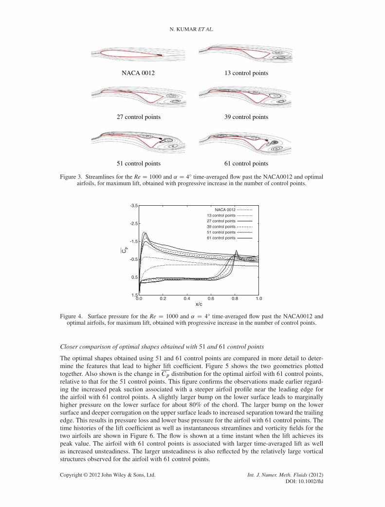
Time-averaged streamlines
Figure 3 shows the time-averaged streamlines for the flow past the optimal airfoils obtained withdifferent numbers of control points. Also shown in the figure is the flow for the NACA0012 airfoil.The flow, on the NACA0012 and the optimal shape obtained with 13 control points, stays attachedon the entire surface except for a small zone of recirculation toward the trailing edge. The optimalairfoil with 27 control points is associated with a corrugation and a recirculation zone on the uppersurface. An additional corrugation and recirculation zone is observed for the optimal airfoil with 39control points. With further increase in the number of control points, the corrugation closer to theleading edge moves upstream and the valley of the one closer to the trailing edge becomes deeper.
Time-averaged surface pressure distribution
To obtain further insight into the increased lift generated by the optimal airfoils with corrugations,the pressure distribution on the surface of the airfoil is studied. Figure 4 shows the Cp distributionfor optimal airfoil obtained with different numbers of control points. Compared with the NACA0012airfoil, all the optimal airfoils are associated with a significantly larger peak suction on the uppersurface and a larger region of higher pressure on the lower surface. The increased peak suction is aconsequence of a sharper nose with a slight droop. The higher pressure on the lower surface is dueto the large bump. These features lead to an overall increase in the time-averaged lift. As the numberof control points increase, the airfoil adapts to sharper nose, increased bump on the lower surfaceand larger corrugations on the upper surface. The increased corrugations lead to larger vortices thatadd to the suction on the upper surface. The increase in lift is accompanied with a reduction in basepressure that leads to an increase in the drag.
Figure 3. Streamlines for the Re D 1000 and ˛ D 4° time-averaged flow past the NACA0012 and optimalairfoils, for maximum lift, obtained with progressive increase in the number of control points.
-3.5
-2.5
-1.5
-0.5
0.5
1.50.0 0.2 0.4 0.6 0.8 1.0
Cp
x/c
NACA 001213 control points27 control points39 control points51 control points61 control points
Figure 4. Surface pressure for the Re D 1000 and ˛ D 4° time-averaged flow past the NACA0012 andoptimal airfoils, for maximum lift, obtained with progressive increase in the number of control points.
Closer comparison of optimal shapes obtained with 51 and 61 control points
The optimal shapes obtained using 51 and 61 control points are compared in more detail to deter-mine the features that lead to higher lift coefficient. Figure 5 shows the two geometries plottedtogether. Also shown is the change in Cp distribution for the optimal airfoil with 61 control points,relative to that for the 51 control points. This figure confirms the observations made earlier regard-ing the increased peak suction associated with a steeper airfoil profile near the leading edge forthe airfoil with 61 control points. A slightly larger bump on the lower surface leads to marginallyhigher pressure on the lower surface for about 80% of the chord. The larger bump on the lowersurface and deeper corrugation on the upper surface leads to increased separation toward the trailingedge. This results in pressure loss and lower base pressure for the airfoil with 61 control points. Thetime histories of the lift coefficient as well as instantaneous streamlines and vorticity fields for thetwo airfoils are shown in Figure 6. The flow is shown at a time instant when the lift achieves itspeak value. The airfoil with 61 control points is associated with larger time-averaged lift as wellas increased unsteadiness. The larger unsteadiness is also reflected by the relatively large vorticalstructures observed for the airfoil with 61 control points.
SHAPE OPTIMIZATION WITH LARGE NUMBER OF DESIGN VARIABLES
-0.4
-0.2
0.0
0.2
0.40.0 0.2 0.4 0.6 0.8 1.0
(Cp) 6
1 -
(C
p) 5
1
x/c
Lower surface
Upper surface
-0.20
-0.10
0.00
0.10
0.20
0.30
0.0 0.2 0.4 0.6 0.8 1.0
51 control points61 control points
(b)
(a)
Figure 5. Re D 1000 and ˛ D 4° flow past the optimal airfoils: (a) optimal airfoils, for maximum lift,obtained with progressive increase in the number of control points for 51 and 61 control points and (b) rel-ative change in the surface pressure coefficient for the time-averaged flow for the airfoil obtained with 61
control points with respect to the one obtained with 51 control points.
5.2.2. ReD 1�104. The proposed scheme is utilized to design high lift airfoils for the ReD 1�104
and ˛ D 4° flow with progressive increase in the number of control points. Table III lists the optimalairfoils along with their aerodynamic performance. The results for the NACA0012 are also included.Compared with the NACA0012 airfoil, the optimal airfoil with 13 control points generates 544%more time-averaged lift. Even though the optimal shape has a larger drag, the increase in lift is largeenough to lead to a very substantial increase in lift-to-drag ratio. This optimal airfoil, obtained with13 control points, is utilized as an initial guess for the optimization cycle with 27 control points. Thedesign leads to an increase in lift by 21%, approximately. The design with 39 control points leadsto a further increase in lift. This shape is associated with fairly large corrugations, especially on theupper surface. Computations with further increase in control points (51 and 61) did not lead to anychange in design. As is observed for ReD 1000, the optimal airfoils are associated with a relativelysharp leading edge. However, unlike the optimal airfoils for ReD 1000, the lower surface does notexhibit a bump toward the trailing edge.
Figure 7 shows the time-averaged streamlines for the NACA0012 and optimal airfoils obtainedwith different numbers of control points. The NACA0012 airfoil is associated with a recirculationzone near the trailing edge on the upper surface. The recirculation zone becomes stronger and movesupstream for the optimal airfoil obtained with 13 control points. A small region of secondary recir-culation is also observed on the upper surface at mid-chord, approximately. With 27 control points,a small valley appears on the upper surface of the airfoil, and the recirculation zone becomes evenlarger. Corrugations appear on the surface of the airfoil with 39 control points. These corrugationslead to stronger secondary recirculation zones. The vortical structures result in higher suction onthe upper surface of the airfoil. This is illustrated in Figure 8, which shows the variation of the
Figure 6. ReD 1000 and ˛ D 4° flow past the optimal airfoils, for maximum lift, obtained with progressiveincrease in the number of control points for 51 (left) and 61 (right) control points: (a) time histories of the liftcoefficient for the fully developed unsteady flow and instantaneous (b) streamlines and (c) vorticity fields.
The time instant at which the flow is shown corresponds to the maximum lift for the respective shapes.
Table III. ReD 1� 104 and ˛ D 4° flow past the optimal airfoil: time-averaged lift and drag coefficients ofthe NACA0012 and optimal airfoils, for maximum lift, obtained with progressive increase in the number of
control points.
Airfoil Cl Cd Cl/Cd Shape
NACA0012 0.159 0.050 3.18
13 control points 1.008 0.072 14.00
27 control points 1.217 0.080 15.21
39 control points 1.394 0.104 13.40
time-averaged pressure distribution on the airfoil surface. The pressure on the lower surface doesnot vary much with the increase in control points; the increase in lift is mostly due to the corrugationson the upper surface of the airfoil.
5.2.3. Mesh convergence. The optimal shape obtained for 13 control points at Re D 1 � 104 and˛ D 4° is verified via a mesh convergence study. We refer to the base mesh, with 44,804 nodesand 89,304 elements, as mesh M1. A more refined mesh, mesh M2, consisting of 74,953 nodes and
SHAPE OPTIMIZATION WITH LARGE NUMBER OF DESIGN VARIABLES
13 control pointsNACA 0012
27 control points 39 control points
Figure 7. Streamlines for the ReD 1�104 and ˛ D 4° time-averaged flow past the NACA0012 and optimalairfoils, for maximum lift, obtained with progressive increase in the number of control points.
-3.5
-2.5
-1.5
-0.5
0.5
1.50.0 0.2 0.4 0.6 0.8 1.0
Cp
x/c
NACA 001213 control points27 control points39 control points
Figure 8. Surface pressure for the Re D 1 � 104 and ˛ D 4° time-averaged flow past the NACA0012 andoptimal airfoils, for maximum lift, obtained with progressive increase in the number of control points.
0.00
0.04
0.08
0.12
0.16
-1 -0.9 -0.8 -0.7 -0.6 -0.5 -0.4 -0.3 -0.2 -0.1 0
y/c
x/c
mesh M1mesh M2
Figure 9. Optimal airfoils obtained for lift maximization at Re D 104 and ˛ D 4° with two different finiteelement meshes.
149,602 elements is used to verify the results obtained from the present computations. The optimalshape obtained with 13 control points, with mesh M1, is used as the initial condition for the shapeoptimization to be conducted with mesh M2. The objective is the maximization of time-averagedlift. It is observed that computations with both the meshes lead to the same optimal shape. The twoshapes are shown in Figure 9. Figure 10 shows the time histories of the aerodynamic coefficientswith the two meshes for the optimal shape obtained with the respective meshes. They are virtu-ally identical. The time-averaged aerodynamic coefficients are, therefore, also the same for boththe cases. This exercise demonstrates the adequacy of the mesh resolution in computing optimalaerodynamic shapes.
Figure 10. Shape optimization for lift maximization at Re D 104 and ˛ D 4°: time histories of the (a) liftand (b) drag coefficients for the optimal airfoil shapes obtained with two different finite element meshes.
6. CONCLUSION
A new method is proposed for conducting shape optimization with relatively large number of designvariables. The variation of the objective function with design parameters, for a richer design space, ismost likely associated with more peaks and valleys. As a result, gradient-based methods that searchfor a local optimum do not necessarily lead to a better design as the design space is enriched. Thishas been demonstrated via optimization for maximum lift for the Re D 1000 and ˛ D 4° flow. Theairfoil is represented by fourth-order NURBS, and the control points are used as design variables.When the optimization cycle begins with NACA0012 airfoil, the performance of the optimal airfoilsobtained with 39 and 61 control points are significantly worse than the one obtained with 13 controlpoints. It is, therefore, proposed that the optimization be carried out with progressive increase inthe number of design variables to exploit the richer design space available. Gradual increase in thenumber of design variables ensures that the optimization process does not get stuck in a local opti-mum that has worse aerodynamic performance. The idea is successfully demonstrated with gradualincrease in control points from 13 to 61. For each cycle of optimization, the initial geometry used isthe optimal shape obtained from the previous parameterization. Corrugations on the upper surface ofthe airfoil spontaneously appear as the number of control points are increased. It is to be noted thatthese corrugations cannot be sustained by lower order parameterization with fewer control points.The corrugated upper surface of the airfoil is responsible for the generation of vortical structuresthat lead to enhanced suction and increased lift. The method is also tested for designing a high liftairfoil for the ReD 1�104 flow. As is observed for the ReD 1000 flow, corrugations spontaneouslyappear for the optimal airfoil with relatively large number of control points. The computations showthat there is merit in further investigating airfoils with corrugations.
REFERENCES
1. Mohammadi B, Pironneauj O. Shape optimization in fluid mechanics. Annual Review of Fluid Mechanics 2004;36:255–279.
2. Giles MB, Pierce NA. An introduction to the adjoint approach to design. Flow, Turbulence and Combustion 2000;65:393–415.
SHAPE OPTIMIZATION WITH LARGE NUMBER OF DESIGN VARIABLES
3. Jameson A. Aerodynamic design via control theory. Journal of Scientific Computing 1988; 59:117–128.4. Anderson WK, Venkatakrishnan V. Aerodynamic design optimization on unstructured grids with a continuous
adjoint formulation. Computers and Fluids 1999; 28:443–480.5. Okumura H, Kawahara M. Shape optimization of a body located in incompressible Navier–Stokes flow based on
optimal control theory. Computer Modelling in Engineering and Sciences 2000; 1:71–77.6. Mohammadi B. Optimization of aerodynamic and acoustic performances of supersonic civil transports. International
Journal For Numerical Methods In Fluids 2004; 14:891–907.7. Reuthers J, Jameson A, Farmer J, Martinelli L, Saunders D. Aerodynamic shape optimization of complex aircraft
configurations via adjoint formulations, 1996. AIAA Paper 96–0094.8. Jameson A. Computational aerodynamics for aircraft design. Science 1989; 245:361–371.9. Nadarajah S, Soucy O, Balloch C. Sonic boom reduction via remote inverse adjoint approach, 2007. AIAA Paper
07–0056.10. Soto O, Lohner R, Yang C. An adjoint-based design methodology for CFD problems. International Journal of
Numerical Methods for Heat and Fluid Flow 2004; 14:734–759.11. Abraham F, Behr M, Heinkenschloss M. Shape optimization in steady blood flow: a numerical study of non-
Newtonian effects. Computer Methods in Biomechanics and Biomedical Engineering 2005; 8:127–137.12. Srinath DN, Mittal S. Optimal airfoil shapes for low Reynolds number flows. International Journal for Numerical
Methods in Fluids 2008; 61:355–381.13. Srinath DN, Mittal S. A stabilized finite element method for shape optimization in low Reynolds number flows.
International Journal for Numerical Methods in Fluids 2007; 54:1451–1471.14. Srinath DN, Mittal S, Manek V. Multi-point shape optimization of airfoils at low Reynolds numbers. Computer
Modelling in Engineering and Sciences 2009; 51:169–190.15. Srinath DN, Mittal S. An adjoint method for shape optimization in unsteady viscous flows. Journal of Computational
Physics 2010; 229:1994–2008.16. Srinath DN, Mittal S. Optimal aerodynamic design of airfoils in unsteady viscous flows. Computer Methods in
Applied Mechanics and Engineering 2010; 199:1976–1991.17. Diwakar A, Mittal S. Aerodynamic shape optimization of airfoils in unsteady flow. Computer Modelling in
Engineering and Sciences 2010; 69:61–89.18. Liebeck RH, Ormsbee AI. Optimization of airfoils for maximum lift. Journal of Aircraft 1970; 7:409–415.19. Liebeck RH. A class of airfoils designed for high lift in incompressible flow. Journal of Aircraft 1973; 10:610–617.20. Selig MS, Guglielmo JJ. High lift low Reynolds number airfoil design. Journal of Aircraft 1997; 34:72–79.21. Cerra DF, Katz J. Design of high lift, thick airfoil for unmanned aerial vehicle applications. Journal of Aircraft 2008;
45:1789–1793.22. Tezduyar TE, Mittal S, Ray SE, Shih R. Incompressible flow computations with stabilized bilinear and linear equal-
order-interpolation velocity-pressure elements. Computer Methods in Applied Mechanics and Engineering 1992;95:221–242.
23. Byrd RH, Lu P, Nocedal J, Zhu C. A limited memory algorithm for bound constrained optimization. SIAM Journalof Scientific Computing 1995; 16:1190–1208.
24. Vargas A, Mittal R, Dong H. A computational study of the aerodynamic performance of a dragonfly wing section ingliding flight. Bioinspiration and Biomimetics 2008; 3(026004):1–13.
25. Levy D-E, Seifert A. Simplified dragonfly airfoil aerodynamics at Reynolds numbers below 8000. Physics of Fluids2009; 21(071901):1–17.