1

A Mixed-Integer Linear Programming Model for Optimizing the Scheduling and Assignment of Tank Farm Operations Sebastian Terrazas-Morenoa, Ignacio E. Grossmanna*, John M. Wassickb aCarnegie Mellon University, 5000 Forbes Ave, Pittsburgh PA 15232, USA bThe Dow Chemical Company, 1776 Building, Midland, MI 48674, USA

Abstract

This paper presents a novel mixed-integer linear programming (MILP) formulation for

the Tank Farm Operation Problem (TFOP), which involves simultaneous scheduling of

continuous multi-product processing lines and the assignment of dedicated storage tanks

to finished products. These products are not allowed to mix in storage tanks. Therefore,

once an assignment is made, it has to be maintained until the end of the operating

horizon. Since all products processed by finishing lines have to go into the tank farm

before being shipped, there is the potential to run out of storage, ultimately impacting the

throughput of the finishing lines, a condition known as blocking. The objective of the

problem is to minimize blocking of the finished lines by obtaining an optimal schedule

and an optimal allocation of storage resources. The scheduling part of the model is based

on the Multi-operation Sequencing (MOS) model by Mouret et al., (2011). The

formulation is tested in three examples of different size and complexity. The possibility

of incorporating the MILP model into a decision support system in combination a

Discrete Event Simulation (DES) model of a tank farm is also discussed.

Keywords: Tank farm operation, production scheduling, tank assignment, multi-

operation sequencing.

Introduction

Chemical manufacturing sites ship finished products to customers using different modes

of transportation (MOT) such as railcars, tank trucks, and pipelines. These MOTs are

usually loaded from or connected to storage tanks. Consequently, all finished products

have to be fed from the process into the storage tanks before being shipped to customers.

This type of operation imposes the need for available storage space at all times in order to

2

avoid unnecessary shut-downs of the upstream chemical process. When these shutdowns

occur, they are said to be a result of storage tanks blocking the process. If the chemical

process produces several products and each one requires dedicated tanks, the product-

tank assignment and the processing schedule at the finishing lines determines how

efficiently the storage space is used. An inefficient assignment of tanks or processing

schedule can result in blocking the production of certain products, even when there is

plenty of available storage space in tanks assigned to other products.

In this paper, we consider a multiproduct manufacturing facility that includes finishing

lines connected to a number of storage tanks from which products are shipped to

customers using different modes of transportation (MOT). The tanks are dedicated to one

product, meaning that once a product is assigned to a tank, it cannot be used for another

product. Cleaning of tanks to store different products is not allowed. We are concerned

with finding the best possible assignment of products to dedicated storage tanks, and the

best processing schedule at the finishing lines in order to minimize the unallocated

production. For scheduling purposes, there is a set of production orders that requires the

processing of a certain amount of product in the finishing lines. Orders have a known

release date and all are due at the end of the time horizon. The release date corresponds to

the moment when a certain amount of an unfinished product becomes available for

processing in the finishing lines. These lines can process the order immediately and feed

the storage tanks, or delay the order for a while until there is available storage space. The

main decisions in this problem are the tank-product assignment and the scheduling of

processing orders. The set of storage tanks included in the production facility is

collectively known as a Tank Farm, and therefore, the problem outlined above is referred

to in this paper as the Tank Farm Operation Problem (TFOP).

The paper by Sharda and Vazquez (2009) illustrates the relevance of the tank farm

operation problem (TFOP) for the Dow Chemical company. The authors describe the

development of a Decision Support System to evaluate the operation of a tank farm at a

chemical production site in Freeport, TX. The system they propose is based on Discrete

Event Simulation (DES). In discrete event models the system changes states as events

3

occur and only when those events occur (ExtendSim, 2007). DES works by representing

the occurrence of an event by generating and passing items among the elements of the

simulation model. Cassandras et al. (1993), Banks et al. (2005), and ExtendSim (2007)

are useful references on Discrete Event Systems and Discrete Event Simulation. Sharda

and Vazquez (2009) evaluated the operation of a tank farm in a Dow Chemical site that

consists of more than 80 tanks for storing 60 product families, processed in 6 finishing

lines. Their simulation model captures complex operating constraints, such as the effect

of recycle lines on the simultaneous loading and unloading of tanks, operational logic

when dealing with delayed processing orders, and the stochastic nature and dynamics of

the operation of loading from tanks unto the different modes of transportation (MOT).

Since the approach is based on simulation, it is not intended for finding an optimal

resource allocation or production schedule; it is a tool for evaluating different storage

tank allocations for a given production schedule.

Other authors have used this type of DES as a support tool for operating a tank farm.

Chen et al. (2002) from the Mathematical Modeling Group at BASF provide another

example of a DES study of logistics in a chemical plant. The tank farm problem is also

relevant in crude refining operations. For instance, Stewart and Trierwiler (2005) carried

out a study of the tankage requirement in different operational scenarios for the Kuwait

National Petroleum Company. Their main tool is DES which they combine with Linear

Programming (LP). Chryssolouris et al. (2005) present an integrated simulation based

approach that manages scheduling, tank farm, inventory, and distillation operations in a

refinery. Their approach is based on generating random solutions within a given search

space and evaluating them using the simulation model.

Mathematical programming is another approach to the Tank Farm Operation Problem

(TFOP). Optimization methods can determine the best possible tank allocation and/or

production schedule within a given search space, as opposed to simulation tools that

require the allocation and schedule to be specified. The disadvantage of this approach is

that it requires operational constraints to be expressed as algebraic equations. Many of the

operational constraints of TFOP have to be simplified in order to express them with

4

algebraic equations for the optimization algorithms. Even with this limitation,

optimization approaches have been successfully used in problems related to storage tank

allocation and tank transfer scheduling. Hvattum et al. (2009) addressed the storage tank

allocation problem (TAP) in a maritime bulk shipping operation. A ship is equipped with

a set of storage tanks that are loaded and unloaded according to a scheduled route. This

problem has similar constraints as the tank farm operation problem we address in this

paper; each tank holds only one type of product and several tank-product assignments are

infeasible due to structural or safety constraints. The loads received and delivered at

different ports are similar to product loading and unloading to storage vessels in the tank

farm according to a production and shipping schedule. A Mixed-integer Linear

Programming (MILP) model is used to either test the feasibility of a shipping route, to

minimize tank cleanup time, or to maximize the vacant space in storage tanks. The main

difference between the TAP and the TFOP is that the TFOP deals with a continuous

production system, whereas the TAP deals with a limited number of discrete loading and

unloading events. The work by Ha et al. (2000) is a good example of a research topic

related with storage tank allocation, namely, the optimization of intermediate buffer

sizing and allocation in multi-product batch process systems. Ha et al. (2000) determine

the location, number, and size of storage tanks with the objective of minimizing the

makespan. As opposed to the Tank Farm Operation Problem (TFOP), storage vessels can

be shared by different types of batches. Vecchietti and Montagna (1998) address a similar

problem.

From the above review, we can conclude that Discrete Event Simulation (DES) is the

approach that has received the most attention for addressing the TFOP in process

industries. Mathematical optimization has been mostly aimed at related problems such as

buffer tank allocation in multiproduct batch scheduling, or to assignment problems such

as in the case of the tank allocation problem in maritime operations. Some authors (Zeng

and Yang, 2009; Chen et al., 2002) have correctly pointed out that the number of

variables and constraints, the operational complexity, and the stochastic nature of logistic

processes involved in tank farm management produce either intractable or oversimplified

mathematical optimization models. Zeng and Yang (2009) proposed integrating

5

simulation and optimization for solving the TFOP. Their argument is that an approximate

optimization model is sufficient for obtaining good solutions that can be evaluated using

the simulation model in a second step. They used neural networks and genetic algorithms

for the optimization module.

The objective of this paper is to present an optimization method based on mathematical

programming, namely Mixed-Integer Programming (MILP), for solving the TFOP. Our

model of the TFOP includes scheduling of orders that arrive to the finishing lines as well

as the optimal tank allocation. We use the description of the tank farm operation given by

Sharda and Vazquez (2009), and try to incorporate in our MILP model as much of the

operational details as possible. This paper does not include simulation by DES.

Nevertheless, we believe that the output of the optimization model we propose could be

evaluated, validated, and communicated using DES.

In the following sections of this paper we give a more detailed description of the tank

farm problem, state the optimization problem, discuss the mathematical model, and apply

the formulation to three case studies. We end this paper with a summary of our findings

and a discussion of possible future work.

Problem Statement

A downstream section of a chemical production facility includes a set M of continuous

finishing lines that represent the last step in the manufacturing of a set J of products,

along with a set K of storage tanks (the tank farm) from where the products are shipped

to the consumers. The shipping operation uses different modes of transportation, usually

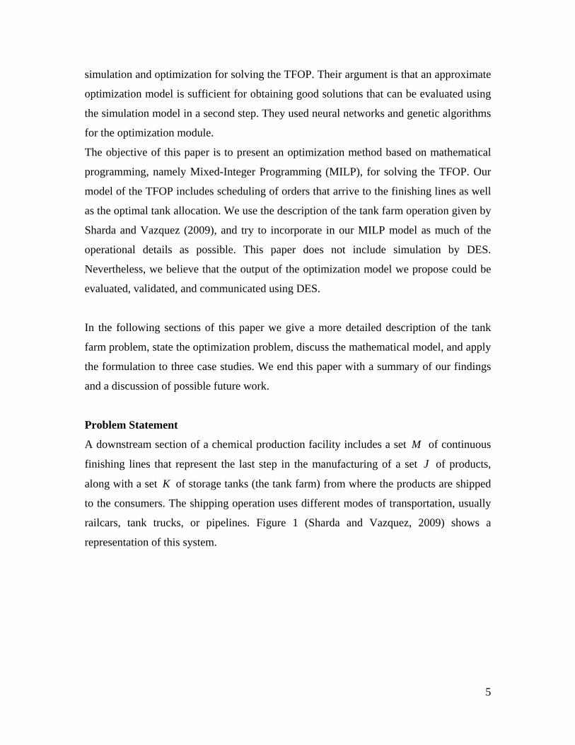
railcars, tank trucks, or pipelines. Figure 1 (Sharda and Vazquez, 2009) shows a

representation of this system.

6

Fig. 1 Downstream section of chemical production process

The processing step in lines Mm is carried out according to processing orders. A

processing order is generated when a batch of unfinished product from the upstream

chemical plant is ready to be processed by the finishing lines, which operate

continuously. The parameter jod , specifies the amount of product j to be produced

according to order o . Each order Oo has a release date ord that corresponds to the

moment when the unfinished product is available for processing in the finishing lines,

and when the corresponding production order gets generated. All orders are due at the

end of the operating horizon. If an order cannot be processed at its release date, its

production can be delayed as long as it can still meet the due date. The production rate of

each product Jj in line m , mjrate , , is a known deterministic parameter. After its

release date, ord , the order o is processed in the finishing lines and sent to storage in one

of the Kk tanks of the tank farm. At the beginning of the time horizon, some or all of

the tanks are empty. However, once a tank k has been allocated to store a product j , it

remains dedicated to this product throughout the operating horizon considered in this

paper. One of the biggest operational challenges of this problem is that an order cannot be

processed and transferred to a tank, unless there is available space in the tanks. When

transfer is not possible and the production order has to be delayed, it is said that tanks are

FinishingTrain

FinishingTrain

Product A Product A

Product B Product C

Railcar

Tank Truck

Railcar

Tank Truck

RailcarRailcar

Tank TruckTank Truck

Process Tanks

FinishingTrain

FinishingTrain

Product A Product A

Product B Product C

Railcar

Tank Truck

Railcar

Tank Truck

RailcarRailcar

Tank TruckTank Truck

Process Tanks

Upstream chemical process

7

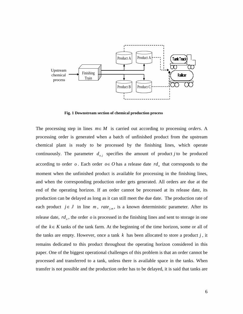
blocking the finishing lines. In this case the processing of orders in the finishing lines has

to be rescheduled.

Figure 2 is adapted from Sharda and Vazquez (2009); it shows the operational logic for

processing production orders and transferring finished product into storage tanks.

Fig. 2 Operational logic in tank farm simulation model

Since the time horizon is finite, blocking and delaying or orders ultimately results in

some orders that cannot be produced. Such unsatisfied orders generate unallocated

product at the end of the time horizon. The main decisions that this paper is concerned

with are the assignment of finished products to storage tanks, and the scheduling of

production orders.

There are a number of operational characteristics that make the management of an actual

tank farm a complex problem. The processing of certain products might not be possible

in every finishing line, and a product can only be transferred from a line to a tank if there

is piping or some other type of connection between them. Simultaneous loading and

unloading is prohibited for some tanks. Finally, shipping can be done using different

Start finishing process

Select tankdedicated to the product requested by the order

Load product from finishing train into tank

Hold until minimum quantity reached

Hold until tank is full or lot is complete

Unload product from tank

Record unsatisfied

quantity

All order quantity assigned

Start processing next order

Yes

No

Tank full/ order complete

Minimum quantity reached

Tank capacity reached

Tank capacity reached

All tanks searched

Release tank

All product unloaded

YesSimultaneous loading and unloading

NO Simultaneous loading and unloading

8

modes of transportation (MOTs), namely, railcars and tank trucks that are loaded in

batches at specified times that correspond to the arrival of available MOTs.

The problem can be summarized as follows:

Given are:

A finite time horizon

A set of finishing lines and their operational characteristics:

o Subset of products that can be processed in it

o Processing rate for each product

o Subset of tanks that the line is connected to, and to which it can transfer

material

A set of production orders with the following information:

o Product to be processed

o Quantity of product to be processed

o Release date

o A due date corresponding to the end of the operating horizon

A set of products

A set of storage tanks and their characteristics:

o Maximum capacity (volume or mass)

o Subset of products that are compatible with its operating conditions

o Frequency of unloading to MOT

o Rate of transfer to MOT during unloading

The simplifications with respect to realistic tank farm operation are as follows:

Unloading operations occur at the same time in all tanks. Otherwise, the

unloading of each tank at the end of each day could potentially require a priority

slot (defined later in the paper), and the problem size would increase

considerably.

Simultaneous loading and unloading of tanks is prohibited.

9

Modes of transportation operate in semi continuous mode only; there are no

continuous MOTs.

Changeover times are neglected for the scheduling.

The problem is to determine:

The assignment of products to dedicated storage tanks

The assignment of orders to finishing lines

The start and duration of the processing time for each order

The tank or tanks to which each order will be transferred to

Subject to:

Assignment constraints:

o One product per tank

o Maximum and minimum number of tanks for a product

o Physical and chemical compatibility of finished product and tank

conditions

o Constraints given by existing connections between finishing lines and

storage tanks

Mass balance constraints

o The rate of processing of an order is equal to the rate of transfer to storage

tanks

o Accumulation in storage tanks is equal to all transfers from lines minus all

quantity loaded to MOTs

Scheduling constraints

o No two orders can be processed simultaneously in the same line

o An order can only be processed after its release date

Tank operation constraints

o Simultaneous loading and unloading is not allowed for some tanks

o Unloading operations to MOTs occur with predetermined frequency

o Unloading operations to MOTs have a predetermined maximum duration

10

With the objective of:

Minimizing unallocated production that results from blocking finishing lines by

unavailability of storage space

Continuous time scheduling in the Tank Farm Operation Problem (TFOP)

The fact that production orders can be delayed, allows for optimization of the processing

schedule at the continuous finishing lines. An important characteristic of the finishing

process is that once an order has started, it has to be processed completely or the

unprocessed quantity has to be declared as unallocated product. This fact is a result of the

operational logic shown in Figure 2.

There are alternative models that can be used for scheduling continuous parallel

production lines. Since we are interested in the material balance in the storage tanks, we

need to consider the transfer of different products from several parallel finishing lines.

The simplest alternative to do so is to use a discrete time formulation. The state-task-

network (Kondili et al., 1993) and the resource-task-network (Pantelides, 1994) are the

most general discrete time formulations for batch processes. Since the process at hand is

single-stage and continuous, a much simpler formulation where at most one production

order can be assigned to each time interval and each line could be used. The transfer to

storage tanks would be equal to the processing rate, and the unloading of tanks to MOTs

could also be specified for some of the time intervals. The balance of the inventory tank

could be easily calculated at the end of each time interval. The drawback of this simple

discrete time formulation is that when a large number of time intervals are needed, the

problem may become intractable.

Continuous time scheduling models are now common since they can potentially decrease

the combinatorial complexity that results from discrete time models (Floudas and Lin,

2004). Erdirik-Dogan and Grossmann (2008) present a model for simultaneous planning

and scheduling of continuous parallel production lines that divides the operating horizon

into planning time periods. The inventory mass balance is calculated at the beginning and

11

at the end of each time period. A slot-based MILP scheduling problem in continuous time

is solved within each time period. This model has a very natural way for incorporating

sequence-dependent changeovers that has been extended by Lima et al. (2011) and

Kopanos et al. (2011) to consider production changeovers across time periods. Yet

another type of continuous time models relevant to the TFOP comes from the study of

tank transfer and crude oil scheduling problems in the refining industry (Furman et al.,

2007; Mouret et al., 2009; Mouret et al., 2011 ). Among these alternative models, we use

the Multi-operation Sequencing (MOS) model described by Mouret et. al (2011). In

Appendix A we discuss how the MOS model was chosen over some alternative

formulations.

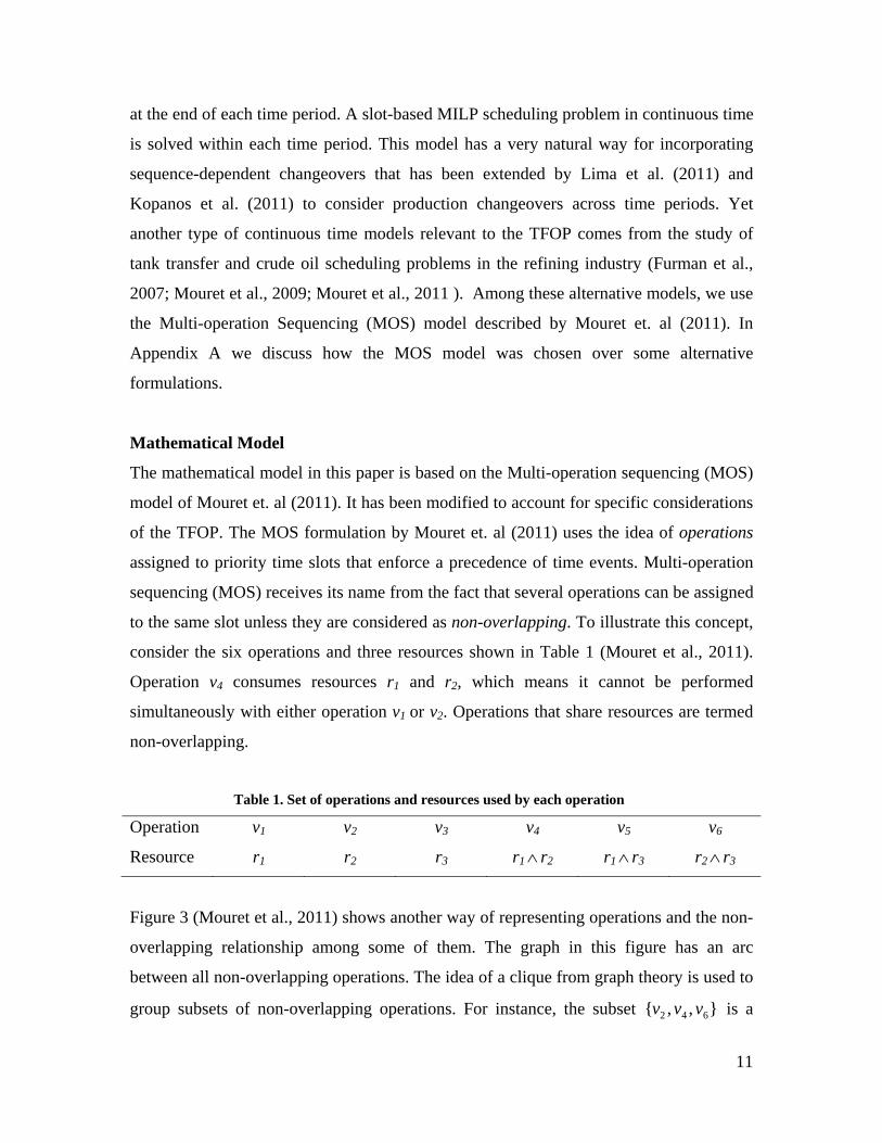
Mathematical Model

The mathematical model in this paper is based on the Multi-operation sequencing (MOS)

model of Mouret et. al (2011). It has been modified to account for specific considerations

of the TFOP. The MOS formulation by Mouret et. al (2011) uses the idea of operations

assigned to priority time slots that enforce a precedence of time events. Multi-operation

sequencing (MOS) receives its name from the fact that several operations can be assigned

to the same slot unless they are considered as non-overlapping. To illustrate this concept,

consider the six operations and three resources shown in Table 1 (Mouret et al., 2011).

Operation v4 consumes resources r1 and r2, which means it cannot be performed

simultaneously with either operation v1 or v2. Operations that share resources are termed

non-overlapping.

Table 1. Set of operations and resources used by each operation

Operation v1 v2 v3 v4 v5 v6

Resource r1 r2 r3 r1 r2 r1 r3 r2 r3

Figure 3 (Mouret et al., 2011) shows another way of representing operations and the non-

overlapping relationship among some of them. The graph in this figure has an arc

between all non-overlapping operations. The idea of a clique from graph theory is used to

group subsets of non-overlapping operations. For instance, the subset },,{ 642 vvv is a

12

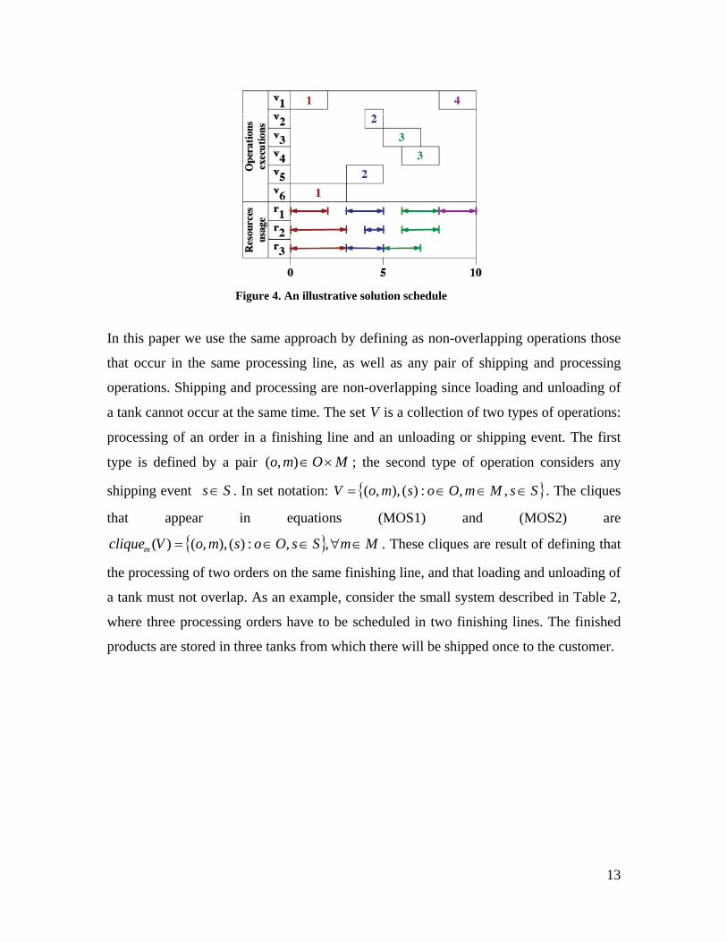
clique in the graph on Figure 3. Figure 4 (Mouret et al., 2011) shows a schedule with the

six operations in Table 1 that illustrates the idea of multi-operation sequencing (MOS)

and non-overlapping operations for a set of 4 priority time slots. For instance, note that

operations 1v and 6v are assigned to slot 1, while operations 2v and 5v are assigned to

slot 2. In general, let V be the set of operations, L the set of slots, ,vS the start of

operation Vv in slot L , ,vE the ending time, and ,vZ a binary equal to 1 if v is

assigned to . Then, the basic idea of the MOS model is summarized by the following

constraints:

1*

, Vv

vZ )(*, VcliqueVL (MOS1)

and

)1(*

,*

,*

, 221

Vv

vVv

vVv

v ZHSE )(*,,,, 2121 VcliqueVL , (MOS2)

where )(Vclique is formed by all subset of operations VV * such that any two

operation in *V must not overlap. For instance, all operations that use a common

resource would be part of a set )(* VcliqueV . Note that constraints (MOS1) states that

at most one operation v from a given subset of operations *V can be assigned to a slot

, while constraint (MOS2) enforces for all operations from the subset *V , that the end

time of slot 1 takes place before the start time of slot 2 if an assignment is made.

Figure 3. Non-overlapping graph

13

Figure 4. An illustrative solution schedule

In this paper we use the same approach by defining as non-overlapping operations those

that occur in the same processing line, as well as any pair of shipping and processing

operations. Shipping and processing are non-overlapping since loading and unloading of

a tank cannot occur at the same time. The set V is a collection of two types of operations:

processing of an order in a finishing line and an unloading or shipping event. The first

type is defined by a pair MOmo ),( ; the second type of operation considers any

shipping event Ss . In set notation: SsMmOosmoV ,,:)(),,( . The cliques

that appear in equations (MOS1) and (MOS2) are

MmSsOosmoVcliquem ,,:)(),,()( . These cliques are result of defining that

the processing of two orders on the same finishing line, and that loading and unloading of

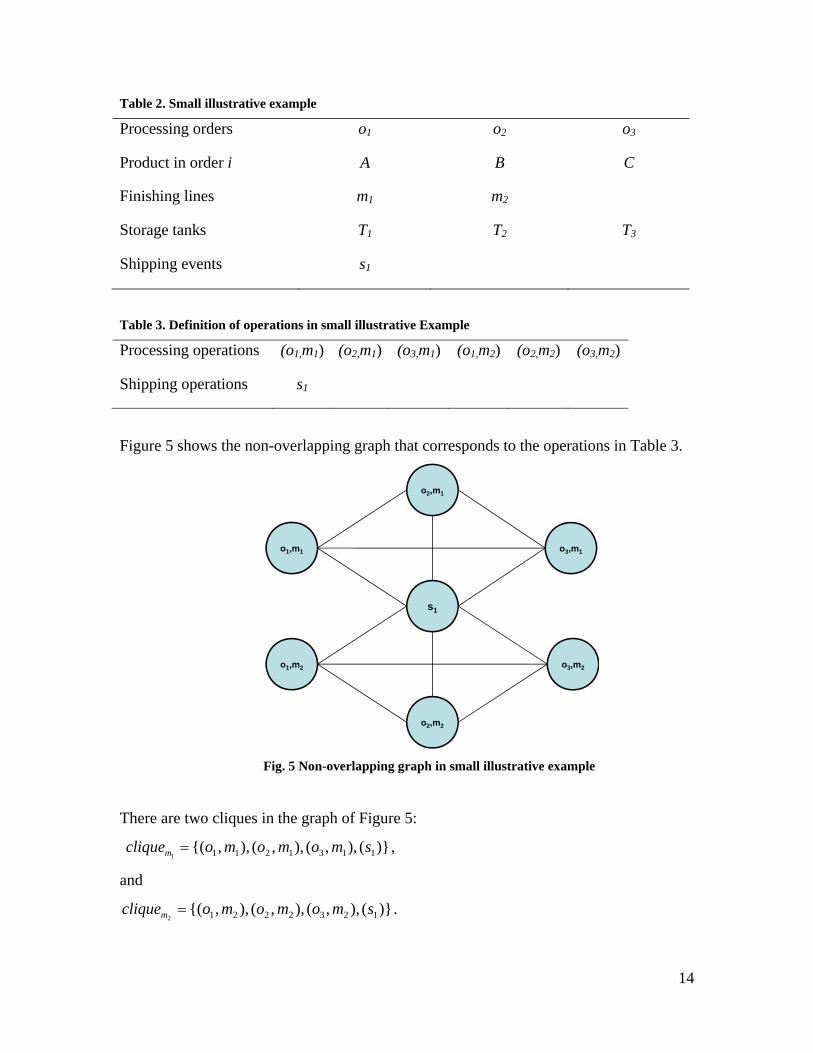
a tank must not overlap. As an example, consider the small system described in Table 2,

where three processing orders have to be scheduled in two finishing lines. The finished

products are stored in three tanks from which there will be shipped once to the customer.

14

Table 2. Small illustrative example

Processing orders o1 o2 o3

Product in order i A B C

Finishing lines m1 m2

Storage tanks T1 T2 T3

Shipping events s1

Table 3. Definition of operations in small illustrative Example

Processing operations (o1,m1) (o2,m1) (o3,m1) (o1,m2) (o2,m2) (o3,m2)

Shipping operations s1

Figure 5 shows the non-overlapping graph that corresponds to the operations in Table 3.

Fig. 5 Non-overlapping graph in small illustrative example

There are two cliques in the graph of Figure 5:

)}(),,(),,(),,{( 11312111smomomocliquem ,

and

)}(),,(),,(),,{( 12322212smomomocliquem .

o2,m2

o2,m1

o1,m2

s1

o3,m1

o3,m2

o1,m1

15

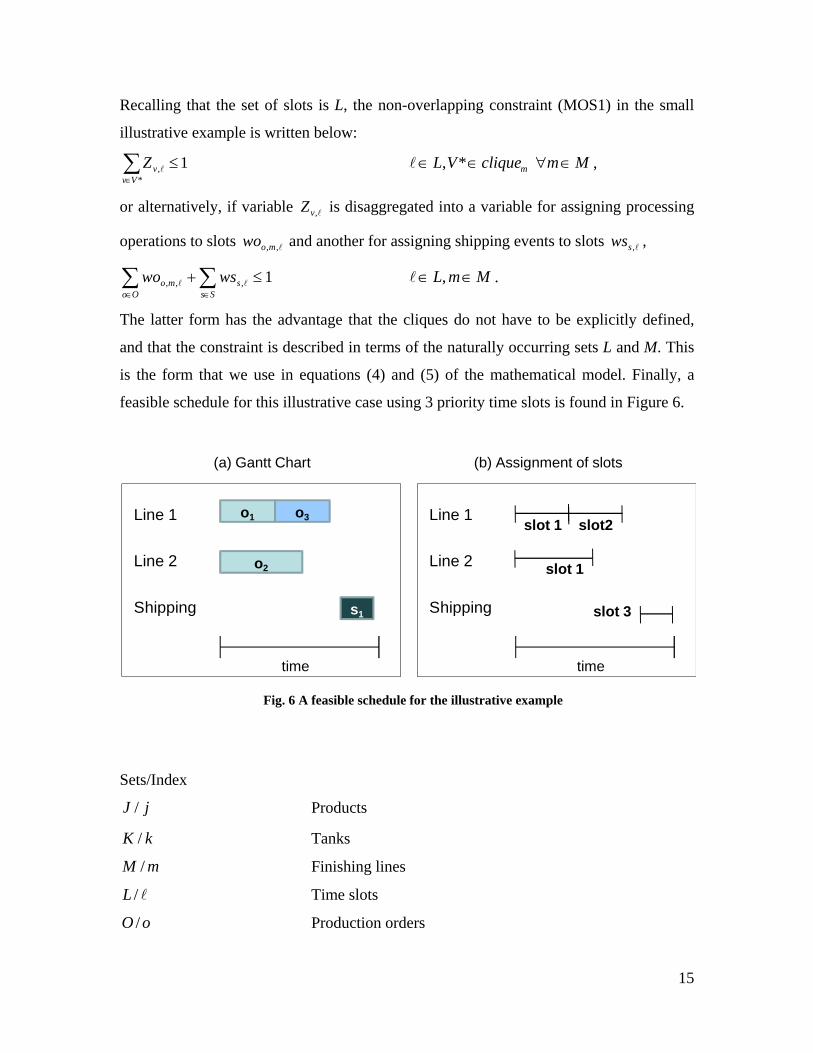
Recalling that the set of slots is L, the non-overlapping constraint (MOS1) in the small

illustrative example is written below:

1*

, Vv

vZ Mm cliqueVL m *, ,

or alternatively, if variable ,vZ is disaggregated into a variable for assigning processing

operations to slots ,,mowo and another for assigning shipping events to slots ,sws ,

1,,, Ss

sOo

mo wswo MmL , .

The latter form has the advantage that the cliques do not have to be explicitly defined,

and that the constraint is described in terms of the naturally occurring sets L and M. This

is the form that we use in equations (4) and (5) of the mathematical model. Finally, a

feasible schedule for this illustrative case using 3 priority time slots is found in Figure 6.

Fig. 6 A feasible schedule for the illustrative example

Sets/Index

jJ / Products

kK / Tanks

mM / Finishing lines

/L Time slots

oO / Production orders

Line 1

Line 2

Shipping

o1 o3

o2

s1

time

(a) Gantt Chart (b) Assignment of slots

Line 1

Line 2

Shipping

slot 1 slot2

slot 1

time

slot 3

16

sS / Shipping or unloading events

Variables

,,mowo binary variable to denote that order o is processed in line

m during slot

,sws binary variable to denote that unloading event s occurs in

slot

kjz , binary variable to denote that tank k is dedicated to

product j

inkmov ,,, quantity of material corresponding to processing order o

transferred to tank k from line m during slot

outksv ,, quantity of material shipped or unloaded from tank k

during unloading event s in slot

klv , inventory levels in tank k at the end of slot

,,mosto start time for processing order o in line m during slot

,ssts start time shipping event s in slot

,,modro duration of processing of order o in line m during slot

,sdrs duration of shipping event s in slot

,,moeo end time for processing order o in line m during slot

,ses end time of shipping event s in slot

ap total amount of finished product allocated to storage tanks

0ks initial inventory in tank k

Parameters

H length of time horizon

kv volume of tank k

17

jo,d amount of finished product j requested by processing

order o

jo, 1 if product j is requested in processing order o ; 0

otherwise

ord release date of processing order o

kjcmp , 1 if physical and chemical properties of product j are

compatible with the operating conditions of tank k; 0

otherwise

kltlc , 1 if any product can be transferred between line and tank

k; 0 otherwise

jmxk maximum number of tanks that can be assigned to product j

jmnk minimum number of tanks that must be assigned to product

j

mjrate , rate of production of product j in line m

jssh , shipping rate of product j in shipping event s

sshd maximum duration of shipping event s

sstime time when a shipping event s is allowed to start; the

maximum shipping event frequency is determined a priori,

according to logistics of modes of transportation

sshipwin time window during which unloading of tank into modes

transportation is allowed; the length of this shipping

window is predetermined by the logistics of the process

system

o Weighting parameter of order o according to its importance

in the production schedule

18

Objective function

The objective is to minimize the unallocated product. This objective is equivalent to

maximizing the amount of finished product that is allocated to the storage tanks during

the time horizon. The parameter o is included to give different weights to different

production orders. For instance, if an order is urgent it could have a large value of o .

For all the results in this paper we set Ooo ,1 .

Oo L Mm Kk

inkmoovap

,,, (obj)

Scheduling constraints

Equations (1a) and (1b) establish that the start time for the processing of order o in line

m at slot is zero if the order is not assigned to that line during that slot, or otherwise it

must be sometime after the release date and before the end of the horizon. Equation (1c)

is a constraint on the frequency of shipping events. This equation fixes the start of each

event s at slot to either zero or the predetermined shipping time sstime . In equation

(1d) the duration of the processing operation of order o in line m can only be non-zero if

has to been assigned to slot . The duration of a shipping event is either zero or less than

the predetermined maximum duration of shipping events, as established by equation (1e).

Equations (1f) and (1g) set the ending time of any slot to either zero if it is not assigned

to processing or shipping, or to less than the operating horizon. Equations (2a) and (2b)

establish that the ending time of any slot is equal to its starting time plus its duration.

Hwosto momo ,,,, MmLOo ,, (1a)

omomo rdwosto ,,,, MmLOo ,, (1b)

sss stimewssts ,, LSs , (1c)

Hwodro momo ,,,, MmLOo ,, (1d)

sss shipwinwsdrs ,, LSs , (1e)

Hwoeo momo ,,,, MmLOo ,, (1f)

Hwses ss ,, LSs , (1g)

19

momomo drostoeo ,,,,,, MmLOo ,, (2a)

,,, sss drsstses LSs , (2b)

It should be noted that the sum of all processing durations modro ,, for each order are

bounded by the sum of the product demands jodo , as will be specified later in constraint

(6).

By constraint (3a) an operation can be assigned at most once to any slot or finishing line;

by constraint (3b) each shipping event only takes place once.

1,, L Mm

mowo

Oo (3a)

1, L

sws

Ss (3b)

Constraint (4) enforces that no overlapping operations are assigned to the same slot. It

was described in more detail in the previous sections.

1,,, Ss

sOo

mo wswo MmL , (4)

According to the idea of priority slots (Mouret et al., 2009), slot 1 in equation (5) has a

higher priority than slot 2 in the sense that it takes place before or at the same time as

slot 2 . If two non-overlapping operations, such as processing on the same finishing line

or a shipping event and a processing operation, are assigned to 1 and 2 , then 2 must

start after the end of 1 . Equation (5) enforces this constraint. The duration of the

intermediate slots 21: is considered in order to strengthen this constraint

(Mouret et al., 2011).

)1(2222

2121

11

,,,,,,

,,,,,,,

smoSs

sOo

mo

Lms

Lmo

Sss

Oomo

wswoHstssto

drsdroeseo

MmL ,,,, 2121 (5)

20

Tank transfer constraint

Equations (6) and (7) allow the transfer of a finished product to storage tank k from line

m during slot , only if an order corresponding to that product is being processed, and if

the tank is assigned to this product (i.e. 1, kjz ) . In both constraints Jj

jod , is a valid

upper bound. Constraint (8) allows transfer between a line and a tank only if there is

feasible connection (e.g., a pipe) between them. Constraint (9) sets the maximum rate of

transfer to tanks equal to the rate of processing at the finishing lines. Equation (10) sets

the maximum amount that can be unloaded from a tank for a shipping event in a given

slot. The maximum rate of unloading is set by constraint (11)

Jj

jomoKk

inkmo dwov ,,,,,, MmLOo ,, (6)

)( ,,,,,

Jj

jokjin

kmo dzv KkMmLOo ,,, (7)

Jj

jomkin

kmo dtlcv ,,,,, KkMmLOo ,,, (8)

Jj

momjjoin

kmo droratev )( ,,,,,,, KkMmLOo ,,, (9)

ksout

ks vwsv ,,, KkLSs ,, (10)

,,,, sjsout

ks drsshv KkLSs ,, (11)

Material balance in storage tanks

The concept of priority slots 21, where,21 ˆ21 stet , allows the material

balance at each tank to be calculated as in constraint (12).

Ss

outks

Mm Oo

inkmok vvlv

11

1

11

1:

,,:

,,,, KkL , (12)

Constraint (13) limits the level of inventory to the capacity of tank k,

kk vlv , KkL , (13)

21

Tank assignment constraints

Equation (14) enforces the condition that at most one product can be assigned to each

dedicated tank. Constraint (15) establishes the minimum and maximum number of tanks

to which a product can be assigned. Constraint (16) allows an assignment only if the

chemical and physical properties of a product are compatible with the operating

conditions of a tank.

1, j

kjz Kk (14)

jk

kjj mxkzmnk , Jj (15)

kjkj cmpz ,, KkJj , (16)

Variable domain specifications

1,0,, mowo MmLOo ,, (17)

1,0, sws LSs , (18)

1,0, kjz KkJj , (19)

outks

inkmo vv ,,,,, , SsKkMmLOo ,,,, (20)

momomo eodrosto ,,,,,, ,, MmLOo ,, (21)

,,, ,, sss esdrssts LSs , (22)

klv , KkL , (23)

ap (24)

Example 1

In this example we wish to determine the optimal tank assignment and optimal schedule

for a system of five tanks and two finishing lines where three products are processed. We

have a set of production orders that arrive during an interval of two weeks. This set of

production orders is representative of the frequency of orders and the quantity ordered

during long term operation of the system. Thus, it can be used for optimally assigning

tanks to products. Tables 4 – 6 contain the data required for the optimization model. In

22

this example we consider that all products can be stored in all tanks, and that there is a

feasible connection between every line and every tank.

Table 4. Production orders in Example 1

Table 5. Production rate and tank capacities in Example 1

Table 6. Interval between shipping, duration of unloading, and unloading rate

The TFOP formulation described in the mathematical model section is used to solve

Example 1. After some pre-analysis, 6 priority time slots are postulated. The main idea is

that we need 4 slots to process the 8 orders in the 2 production lines, and, given the rates

of unloading of tanks, about 2 or 3 slots for shipping operations. Computational results

indicate that 6 priority slots yield the same solution as 7 but require less computational

time. The resulting Mixed-Integer Linear Programming (MILP) model has 195 binary

Order Product

Quantity 

[ton/hr]

Release date 

[hr]

1 A 105 0

2 C 69 0

3 C 35 48

4 B 98 72

5 A 110 96

6 B 56 168

7 C 102 216

8 B 90 264

Tank  

Interval 

[hr]

Duration 

[hr]

Transfer rate 

[ton/hr]

1 24 6 12.07

2 24 6 13.86

3 24 6 12.01

4 24 6 12.31

5 24 6 11.83

23

variables, 1,471 continuous variables, and 3,358 constraints. It was implemented in

GAMS version 23.6 for Windows and solved using CPLEX 12.2 with an Intel Core i7

CPU at 2.93 GHz, and 4.00 GB of RAM. A solution within 0.2% of the optimum was

found in 60 CPU seconds. The results are summarized in Table 7, and Figures 7 – 8. As

seen in Table 7, 1.4 ton of product B cannot be allocated.

Table 7. Allocated product for Example 1

Figure 7 shows the optimal product-tank assignment. The total production volume

specified by the production orders of Product B is the highest, and it is assigned the

largest total storage tank capacity. Product A has a larger production target than product

C, but product A is allotted less storage space. Figure 8 shows that the two production

orders of product A are scheduled at the beginning and end of the time horizon, allowing

for the complete unloading of the storage tank. This fact is observed in Figure 9(d). The

Gantt chart in Figure 8 shows how the scheduling of non-overlapping operations, such as

the processing operations in the same line, and processing and unloading operations are

never scheduled in the same slot. From this figure we can also confirm that the ordering

of the priority slots is maintained: every slot that has a lower numbering than a shipping

slot ends before the shipping starts.

Product

Ordered amount 

[ton]

Allocated  Quanity 

[ton]

A 215 215

B 244 242.6

C 206 206

Total 665 663.6

24

Fig 7. Optimal product-tank assignments in Example 1

Fig. 8 Gantt chart of optimal schedule in Example 1

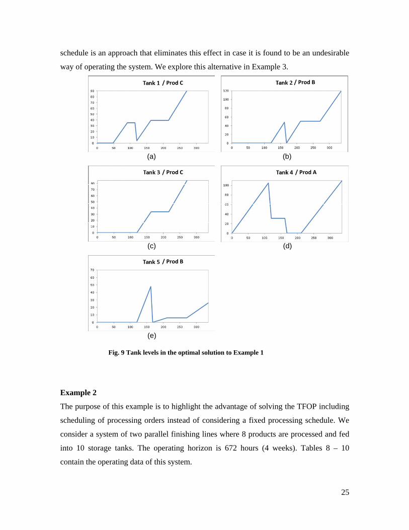
The plots of the tank levels in Figure 9 show a common pattern. Towards the end of the

operating horizon all tanks except number 5 are completely full. This result is a

combination of the objective function of the TFOP that requires a maximal amount of

product going into the tanks, and the finite operating horizon. In real-life operations a

shipping event would probably take place at the end of the time horizon. A cyclic

A

B

C

Tank 1

Tank 2

Tank 3

Tank 4

Tank 5

215ton

244ton

206ton

90ton

120ton

85ton

110ton

70ton

0 hrs 100 200 300 336 hrs

Line 1 order 1 order 2 order 7 order 8 Product A

Line 2 order 3 order 4 order 6 order 5 Product B

Product C

Shipping

Shipping

Line 1

slot 1 slot 3 slot 5 slot 6

Line 2

slot 1 slot 3 slot 5 slot 6

Shipping

slot 2 slot 4

0 hrs 100 200 300 336 hrs

25

schedule is an approach that eliminates this effect in case it is found to be an undesirable

way of operating the system. We explore this alternative in Example 3.

Fig. 9 Tank levels in the optimal solution to Example 1

Example 2

The purpose of this example is to highlight the advantage of solving the TFOP including

scheduling of processing orders instead of considering a fixed processing schedule. We

consider a system of two parallel finishing lines where 8 products are processed and fed

into 10 storage tanks. The operating horizon is 672 hours (4 weeks). Tables 8 – 10

contain the operating data of this system.

(a) (b)

(c) (d)

(e)

/ Prod C

/ Prod C

/ Prod B

/ Prod B

/ Prod A

26

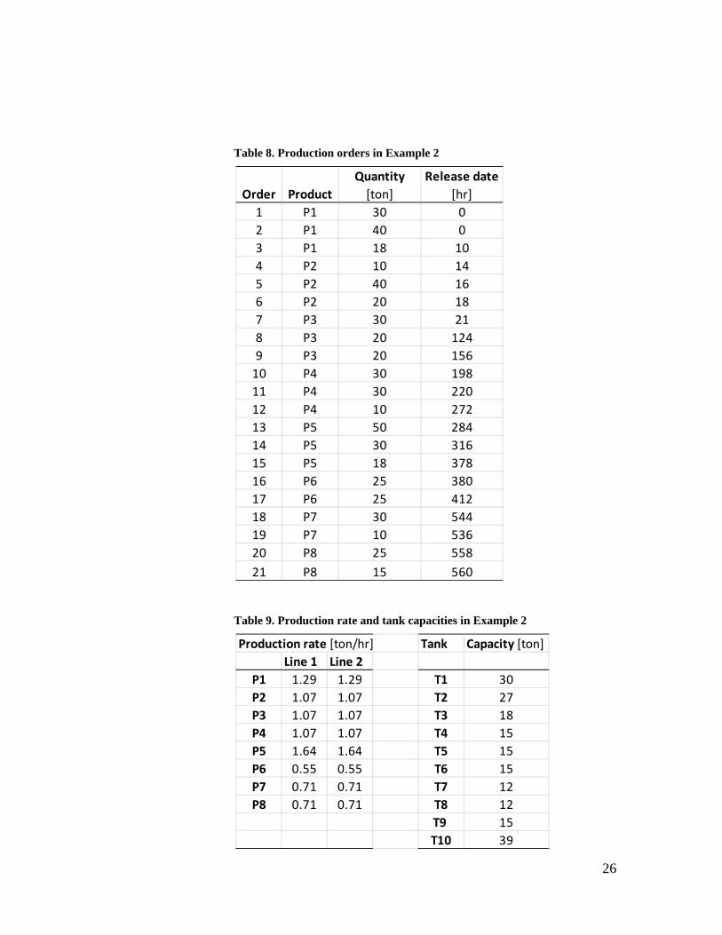
Table 8. Production orders in Example 2

Table 9. Production rate and tank capacities in Example 2

Order Product

Quantity 

[ton]

Release date 

[hr]

1 P1 30 0

2 P1 40 0

3 P1 18 10

4 P2 10 14

5 P2 40 16

6 P2 20 18

7 P3 30 21

8 P3 20 124

9 P3 20 156

10 P4 30 198

11 P4 30 220

12 P4 10 272

13 P5 50 284

14 P5 30 316

15 P5 18 378

16 P6 25 380

17 P6 25 412

18 P7 30 544

19 P7 10 536

20 P8 25 558

21 P8 15 560

Production rate [ton/hr] Tank Capacity [ton]

Line 1 Line 2

P1 1.29 1.29 T1 30

P2 1.07 1.07 T2 27

P3 1.07 1.07 T3 18

P4 1.07 1.07 T4 15

P5 1.64 1.64 T5 15

P6 0.55 0.55 T6 15

P7 0.71 0.71 T7 12

P8 0.71 0.71 T8 12

T9  15

T10 39

27

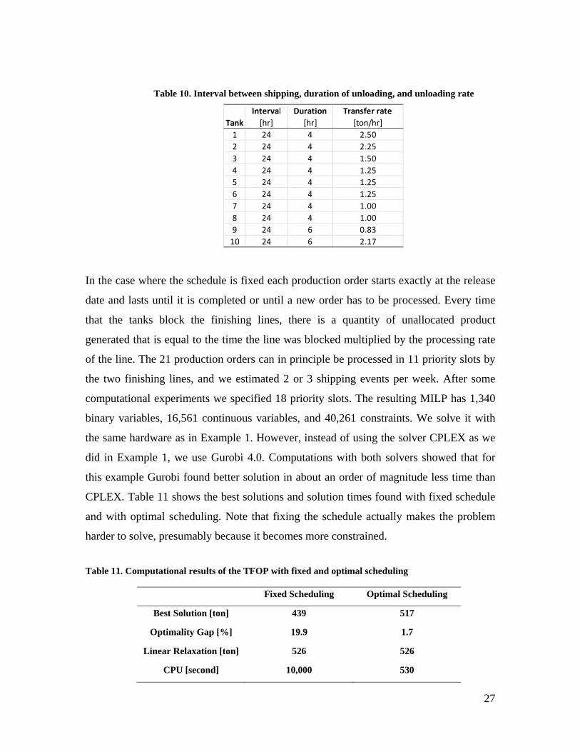
Table 10. Interval between shipping, duration of unloading, and unloading rate

In the case where the schedule is fixed each production order starts exactly at the release

date and lasts until it is completed or until a new order has to be processed. Every time

that the tanks block the finishing lines, there is a quantity of unallocated product

generated that is equal to the time the line was blocked multiplied by the processing rate

of the line. The 21 production orders can in principle be processed in 11 priority slots by

the two finishing lines, and we estimated 2 or 3 shipping events per week. After some

computational experiments we specified 18 priority slots. The resulting MILP has 1,340

binary variables, 16,561 continuous variables, and 40,261 constraints. We solve it with

the same hardware as in Example 1. However, instead of using the solver CPLEX as we

did in Example 1, we use Gurobi 4.0. Computations with both solvers showed that for

this example Gurobi found better solution in about an order of magnitude less time than

CPLEX. Table 11 shows the best solutions and solution times found with fixed schedule

and with optimal scheduling. Note that fixing the schedule actually makes the problem

harder to solve, presumably because it becomes more constrained.

Table 11. Computational results of the TFOP with fixed and optimal scheduling

Tank  

Interval 

[hr]

Duration 

[hr]

Transfer rate 

[ton/hr]

1 24 4 2.50

2 24 4 2.25

3 24 4 1.50

4 24 4 1.25

5 24 4 1.25

6 24 4 1.25

7 24 4 1.00

8 24 4 1.00

9 24 6 0.83

10 24 6 2.17

Fixed Scheduling Optimal Scheduling

Best Solution [ton] 439 517

Optimality Gap [%] 19.9 1.7

Linear Relaxation [ton] 526 526

CPU [second] 10,000 530

28

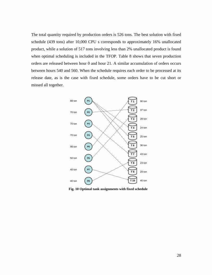
The total quantity required by production orders is 526 tons. The best solution with fixed

schedule (439 tons) after 10,000 CPU s corresponds to approximately 16% unallocated

product, while a solution of 517 tons involving less than 2% unallocated product is found

when optimal scheduling is included in the TFOP. Table 8 shows that seven production

orders are released between hour 0 and hour 21. A similar accumulation of orders occurs

between hours 540 and 560. When the schedule requires each order to be processed at its

release date, as is the case with fixed schedule, some orders have to be cut short or

missed all together.

Fig. 10 Optimal tank assignments with fixed schedule

P3

P5

P8

T 1

T 3

T 5

T 7

T 9

88 ton

P4

P7

P2

P6

P1

T 2

T 4

T 6

T 8

T 10

70 ton

70 ton

70 ton

98 ton

50 ton

40 ton

40 ton

90 ton

37 ton

28 ton

24 ton

25 ton

36 ton

43 ton

23 ton

29 ton

40 ton

29

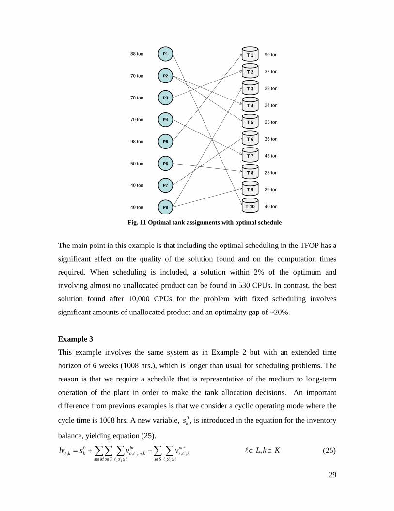
Fig. 11 Optimal tank assignments with optimal schedule

The main point in this example is that including the optimal scheduling in the TFOP has a

significant effect on the quality of the solution found and on the computation times

required. When scheduling is included, a solution within 2% of the optimum and

involving almost no unallocated product can be found in 530 CPUs. In contrast, the best

solution found after 10,000 CPUs for the problem with fixed scheduling involves

significant amounts of unallocated product and an optimality gap of ~20%.

Example 3

This example involves the same system as in Example 2 but with an extended time

horizon of 6 weeks (1008 hrs.), which is longer than usual for scheduling problems. The

reason is that we require a schedule that is representative of the medium to long-term

operation of the plant in order to make the tank allocation decisions. An important

difference from previous examples is that we consider a cyclic operating mode where the

cycle time is 1008 hrs. A new variable, 0ks , is introduced in the equation for the inventory

balance, yielding equation (25).

Ss

outks

Mm Oo

inkmokk vvslv

11

1

11

1:

,,:

,,,0

, KkL , (25)

P3

P5

P8

T 1

T 3

T 5

T 7

T 9

88 ton

P4

P7

P2

P6

P1

T 2

T 4

T 6

T 8

T 10

70 ton

70 ton

70 ton

98 ton

50 ton

40 ton

40 ton

90 ton

37 ton

28 ton

24 ton

25 ton

36 ton

43 ton

23 ton

29 ton

40 ton

30

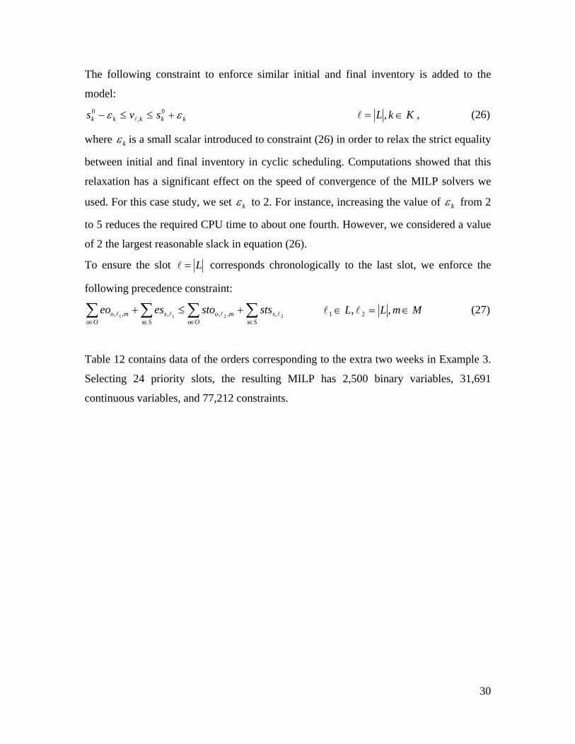
The following constraint to enforce similar initial and final inventory is added to the

model:

kkkkk svs 0,

0 KkL , , (26)

where k is a small scalar introduced to constraint (26) in order to relax the strict equality

between initial and final inventory in cyclic scheduling. Computations showed that this

relaxation has a significant effect on the speed of convergence of the MILP solvers we

used. For this case study, we set k to 2. For instance, increasing the value of k from 2

to 5 reduces the required CPU time to about one fourth. However, we considered a value

of 2 the largest reasonable slack in equation (26).

To ensure the slot L corresponds chronologically to the last slot, we enforce the

following precedence constraint:

Ss

sOo

moSs

sOo

mo stsstoeseo2211 ,,,,,, MmLL ,, 21 (27)

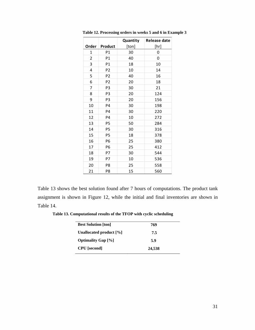
Table 12 contains data of the orders corresponding to the extra two weeks in Example 3.

Selecting 24 priority slots, the resulting MILP has 2,500 binary variables, 31,691

continuous variables, and 77,212 constraints.

31

Table 12. Processing orders in weeks 5 and 6 in Example 3

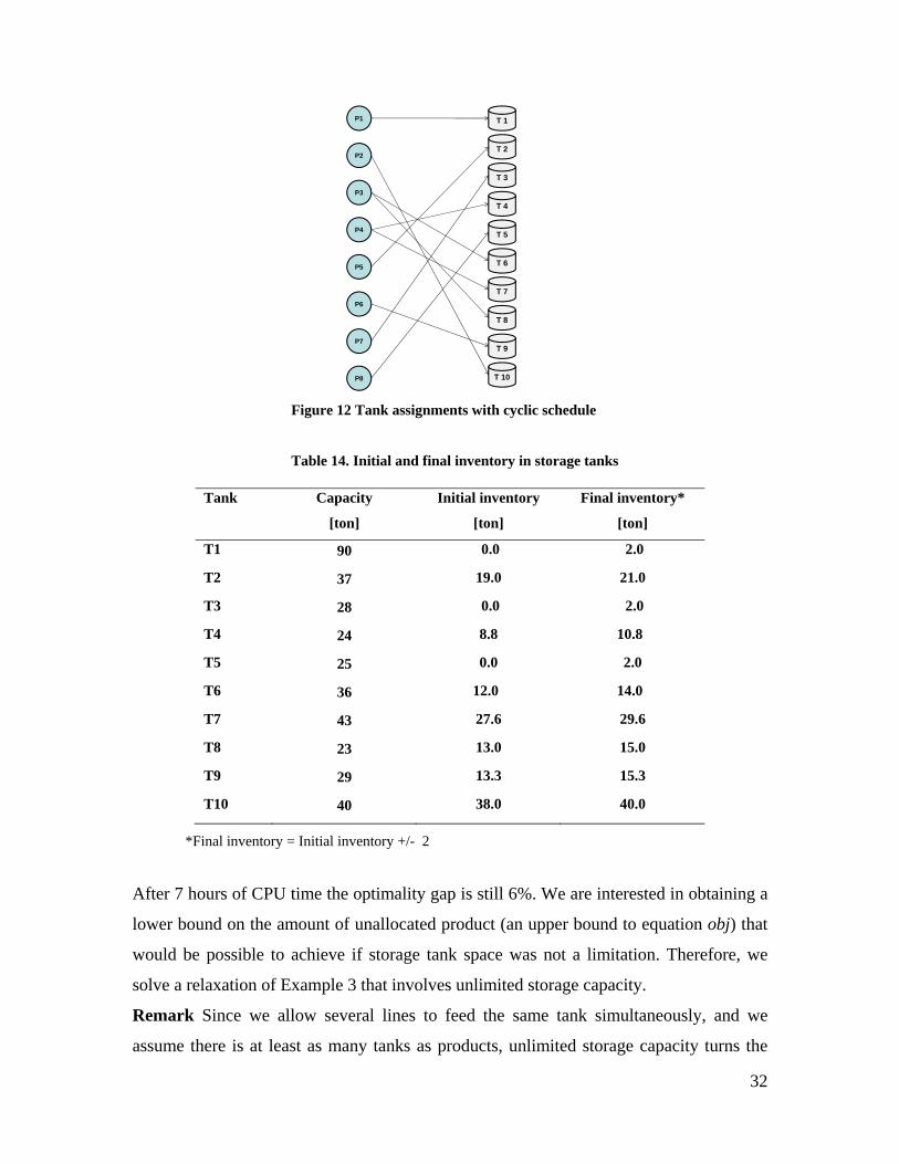
Table 13 shows the best solution found after 7 hours of computations. The product tank

assignment is shown in Figure 12, while the initial and final inventories are shown in

Table 14.

Table 13. Computational results of the TFOP with cyclic scheduling

Order Product

Quantity 

[ton]

Release date 

[hr]

1 P1 30 0

2 P1 40 0

3 P1 18 10

4 P2 10 14

5 P2 40 16

6 P2 20 18

7 P3 30 21

8 P3 20 124

9 P3 20 156

10 P4 30 198

11 P4 30 220

12 P4 10 272

13 P5 50 284

14 P5 30 316

15 P5 18 378

16 P6 25 380

17 P6 25 412

18 P7 30 544

19 P7 10 536

20 P8 25 558

21 P8 15 560

Best Solution [ton] 769

Unallocated product [%] 7.5

Optimality Gap [%] 5.9

CPU [second] 24,538

32

Figure 12 Tank assignments with cyclic schedule

Table 14. Initial and final inventory in storage tanks

*Final inventory = Initial inventory +/- 2

After 7 hours of CPU time the optimality gap is still 6%. We are interested in obtaining a

lower bound on the amount of unallocated product (an upper bound to equation obj) that

would be possible to achieve if storage tank space was not a limitation. Therefore, we

solve a relaxation of Example 3 that involves unlimited storage capacity.

Remark Since we allow several lines to feed the same tank simultaneously, and we

assume there is at least as many tanks as products, unlimited storage capacity turns the

P3

P5

P8

T 1

T 3

T 5

T 7

T 9

P4

P7

P2

P6

P1

T 2

T 4

T 6

T 8

T 10

Tank Capacity

[ton]

Initial inventory

[ton]

Final inventory*

[ton]

T1 90 0.0 2.0

T2 37 19.0 21.0

T3 28 0.0 2.0

T4 24 8.8 10.8

T5 25 0.0 2.0

T6 36 12.0 14.0

T7 43 27.6 29.6

T8 23 13.0 15.0

T9 29 13.3 15.3

T10 40 38.0 40.0

33

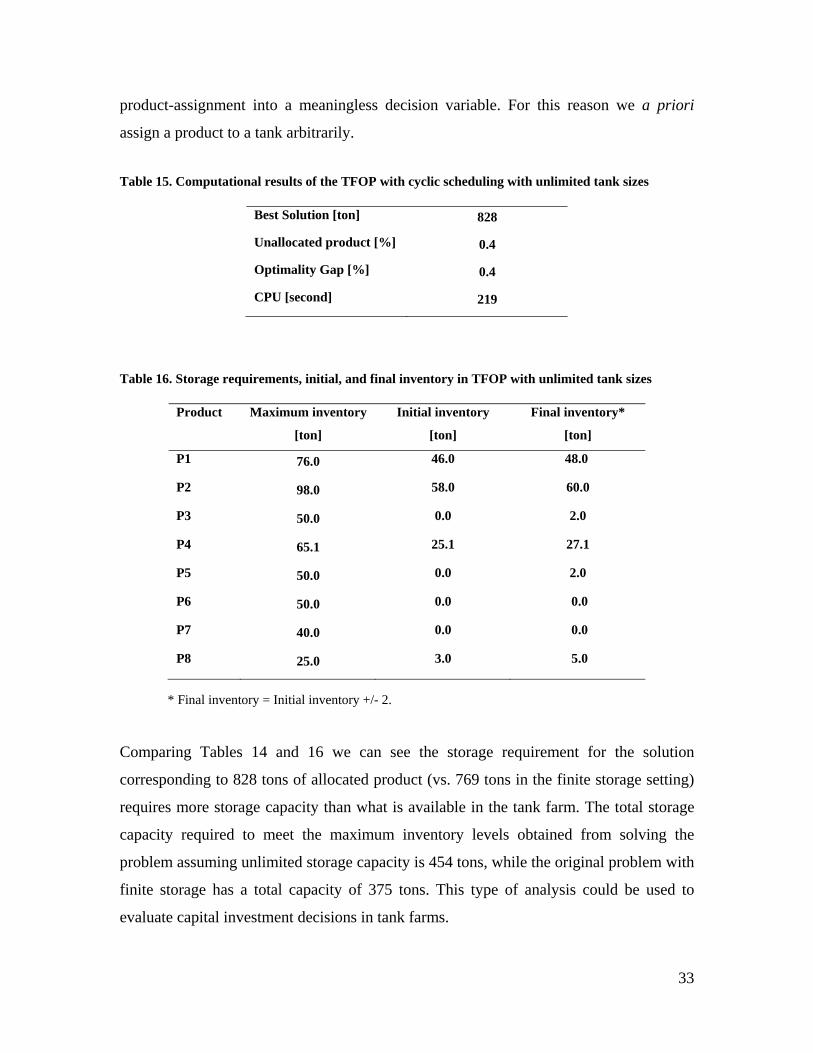
product-assignment into a meaningless decision variable. For this reason we a priori

assign a product to a tank arbitrarily.

Table 15. Computational results of the TFOP with cyclic scheduling with unlimited tank sizes

Table 16. Storage requirements, initial, and final inventory in TFOP with unlimited tank sizes

* Final inventory = Initial inventory +/- 2.

Comparing Tables 14 and 16 we can see the storage requirement for the solution

corresponding to 828 tons of allocated product (vs. 769 tons in the finite storage setting)

requires more storage capacity than what is available in the tank farm. The total storage

capacity required to meet the maximum inventory levels obtained from solving the

problem assuming unlimited storage capacity is 454 tons, while the original problem with

finite storage has a total capacity of 375 tons. This type of analysis could be used to

evaluate capital investment decisions in tank farms.

Best Solution [ton] 828

Unallocated product [%] 0.4

Optimality Gap [%] 0.4

CPU [second] 219

Product Maximum inventory

[ton]

Initial inventory

[ton]

Final inventory*

[ton]

P1 76.0 46.0 48.0

P2 98.0 58.0 60.0

P3 50.0 0.0 2.0

P4 65.1 25.1 27.1

P5 50.0 0.0 2.0

P6 50.0 0.0 0.0

P7 40.0 0.0 0.0

P8 25.0 3.0 5.0

34

Conclusions and future work

We have presented a novel MILP formulation for the Tank Farm Operation Problem

(TFOP) that integrates continuous production scheduling with storage resource allocation

when the storage vessels are dedicated tanks. One of the examples in this paper shows the

impact of including optimal scheduling in the TFOP, as opposed to assuming a fixed

schedule. Even though the scheduling part of the problem corresponds to an efficient

model for continuous-time scheduling based on the idea of Multi-operation Sequencing

(Mouret et al., 2011), the scheduling horizon that can be contemplated within reasonable

computational time is limited to a few weeks. For this reason a representative set of

production orders and release dates has to be chosen in order to obtain an efficient

product-assignment for medium to long-term operation. Alternatively, a cyclic schedule

can be assumed as we did in Example 3.

We envision our MILP formulation combined with Discrete Event Simulation like the

one in Sharda and Vazquez (2009) as part of a comprehensive decision support system.

Consequently, testing and integration with a simulation tool is a natural next step. In this

way the MILP capabilities of rigorous search among alternative could be combined with

the capability for representing complex operational issues of DES.

Acknowledgment

The authors acknowledge Naoko Akiya and Bikram Sharda for their contributions to

defining this problem. The authors are also grateful for the financial support provided by

the Dow Chemical Company.

References

Banks J., J.S. Carson II, B.L. Nelson, and D.M. Nicol (2005). Discrete event system simulations. 4th ed.

Prentice Hall International series in Industrial and Systems. Cassandras C.G. (1993). Discrete Event Systems: Modeling and Performance Analysis. Irwin Publ., 1993. Chen, E.J., M.L. Young, and P.L. Selikson (2002). A simulation study of logistic activities in a chemical

plant. Simulation Modeling practice and Theory, 10, 235 – 245. Chryssolouris G., N. Papakostas, and D. Mourtzis (2005). Refinery short-term scheduling with tank farm,

inventory and distillation management: An integrated simulation based approach. European Journal of Operational Research, 166, 812 – 827.

35

Erdirik-Dogan M. and I. E. Grossmann (2008). Simultaneous planning and scheduling of single-stage multiproduct continuous plants with parallel lines. Computers and Chemical Engineering, 32, 2664 – 2683.

Floudas C.A. and X. Lin (2004). Continuous-time versus discrete-time approaches for scheduling of chemical processes: a review. Computers and Chemical Engineering, 28, 2109 – 2129.

Furman, K.C., Z. Jia, and M.G. Ierapetritou (2007). A robust event-based continuous time formulation for tank transfer scheduling. Industrial and Engineering Chemistry Research, 46, 9126 – 9136.

Ha J., H. Chang, E. S. Lee, In. Lee, B.S. Lee, and G. Yi (2000). Intermediate storage tank operation strategies in the production scheduling of multi-product batch process. Computers and Chemical Engineering, 24, 1633 – 1640.

Hvattum, L.M., K. Fagerholt, V. A. Armentano (2009). Tank allocation problems in maritime bulk shipping. Computers and Operations Research, 36, 3051 – 3060.

Imagine That Inc. (2007). ExtendSim User Guide, Release 7. Kondili E., C.C. Pantelides, and R.W.H. Sargent (1993). A general algorithm for short-term scheduling of

batch operations-I. MILP formulation. Computers and Chemicals Engineering, 2, 211 – 227. Kopanos, G.M., L. Puigjaner, C. T. Maravelias (2011). Production planning and scheduling of parallel

continuous processes with product families. Industrial and Engineering Chemistry Research 50, 1369 – 1378.

Lima, R.M., I.E. Grossmann, and Y. Jiao (2011). Long-term scheduling of a single-unit multi-product continuous process to manufacture high performance glass. Computers and Chemical Engineering 35, 554 – 574.

Mouret S., I.E. Grossmann, and P. Pestiaux (2009). A novel priority-based continuous-time formulation for crude-oil scheduling problems. Industrial and Engineering Chemistry Research, 48, 8515 – 8528.

Mouret S., I.E. Grossmann, and P. Pestiaux (2011).Time representations and mathematical models for process scheduling problems. Computers and Chemical Engineering, 35, 1038 – 1063.

Pantelides, C.C. (1994). Unified frameworks for process planning and scheduling. In Foundations of computer-aided process operations. New York: CACHE publications, pp. 253 – 274.

Sharda B., and A. Vazquez (2009). Evaluating Capacity and Expansion Opportunities at Tank Farm: A Decision Support System using Discrete Event Simulation. Winter Simulation Conference 2009, 2218 – 2224.

Stewart M.D. and L.D. Trierwiler (2005). Simulating optimal tank farm design. PTQ magazine, Q2, 1 – 5. Vecchietti, A.R., J. Montagna (1998). Alternatives in the optimal allocation of intermediate storage tanks in

multiproduct batch plants. Computers and Chemical Engineering, 22(1), S801 – S804. Zeng Q. and Z. Yang (2009). Integrating simulation and optimization to schedule loading operations in

container terminals. Computers and Operations Research, 36, 1935 – 1944.

Appendix A

In this section we present the reasoning for choosing the MOS model over two alternative

scheduling formulations in discrete and continuous time. We base the selection of the

algorithm on the combinatorial complexity of the model measured by the number of

binary variables required in each model.

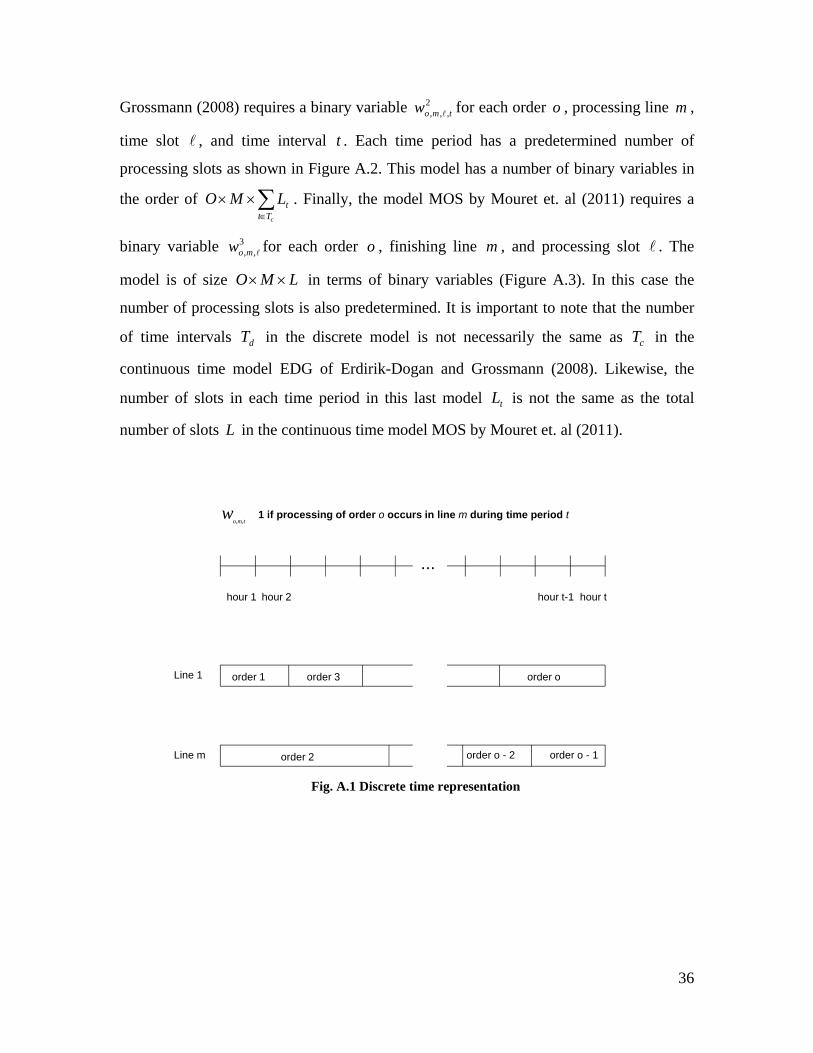
A discrete time model (DTM) requires binary variable 1,, dtmow to indicate the production

of order o in line m during time interval dt . The use of this variable is illustrated in

Figure A.1. The model is of order dTMO . The model EDG by Erdirik-Dogan and

36

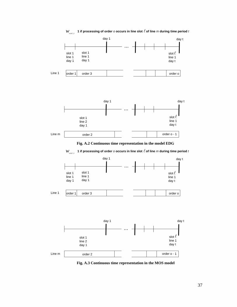
Grossmann (2008) requires a binary variable 2,,, tmow for each order o , processing line m ,

time slot , and time interval t . Each time period has a predetermined number of

processing slots as shown in Figure A.2. This model has a number of binary variables in

the order of

cTt

tLMO . Finally, the model MOS by Mouret et. al (2011) requires a

binary variable 3,, mow for each order o , finishing line m , and processing slot . The

model is of size LMO in terms of binary variables (Figure A.3). In this case the

number of processing slots is also predetermined. It is important to note that the number

of time intervals dT in the discrete model is not necessarily the same as cT in the

continuous time model EDG of Erdirik-Dogan and Grossmann (2008). Likewise, the

number of slots in each time period in this last model tL is not the same as the total

number of slots L in the continuous time model MOS by Mouret et. al (2011).

Fig. A.1 Discrete time representation

o,m,tw

Line 1

Line m

hour 1 hour 2 hour t-1 hour t

...

1 if processing of order o occurs in line m during time period t

order 2 order o - 2 order o - 1

order 1 order 3 order o

37

Fig. A.2 Continuous time representation in the model EDG

Fig. A.3 Continuous time representation in the MOS model

Line m order 2 order o - 1

Line 1 order 1 order 3 order o

to,m,w

,1 if processing of order o occurs in line slot of line m during time period t

day 1 day t

...slot 1line 1day 1

slot 1line 1day 1

slot line 1day t

day 1 day t

...

slot 1line 2day 1

slot line 1day t

Line m order 2 order o - 1

Line 1 order 1 order 3 order o

to,m,w

,1 if processing of order o occurs in line slot of line m during time period t

day 1 day t

...slot 1line 1day 1

slot 1line 1day 1

slot line 1day t

day 1 day t

...

slot 1line 2day 1

slot line 1day t

38

For a given problem with a certain number of orders O to be processed in a set L of

finishing lines, we can estimate the order of the number of binary variables required in

each model. To do so, we exploit certain operational conditions: (i) each order cannot be

split into two processing steps; it has to be completed once it is started, and (ii) shipping

or unloading of the tanks occurs regularly with intervals much smaller than the time

horizon, but larger than the required interval in discrete time optimization. The first

operational condition above allows us to postulate that the maximum number of slots in

the MOS model by Mouret et. al (2011) is at most equal to the number of orders. In the

model EDG by Erdirik-Dogan and Grossmann (2008) we should postulate a number of

processing slots for each time period equal to all the processing orders released before the

start time of the time period. Also, from the operational constraint (ii), we have to impose

that the time intervals cc Tt in the model EDG by Erdirik-Dogan and Grossmann (2008)

coincide with the shipping intervals in order to keep track of inventory levels in storage

tanks. Then, form operational characteristic (ii), we can establish that

dc tthorizon and cd TT .

The number of binary variables in each model is:

dTMODTM

ctTt

t TLMOLMOEDGd

, where tL is the average number of slots

in each time period.

OMOLMOMOS .

Since the number of orders and lines is the same in each model, it is enough to compare

the following quantities: dT , ct TL , and O .

To give a concrete reference to these magnitudes we specify that DTM uses intervals of 4

hours. This means that if the average time between releasing of orders is more than 4

hours then there will be more time intervals in the discrete time model than the total

number of orders. Thus OTd .

39

For the EDG model, we consider that each time interval is one day (unloading of tanks

occurs once a day). We also specify that each week a fixed number of new processing

orders are released. This specification means that a plot of orders released vs. time will be

linear, starting at 0 orders at time 0, and ending with O orders at the end of the time

horizon. Therefore, the average number of orders released per time interval is equal to

2

O. The average number of slots in each time interval in the EDG model can be set equal

to the average number of orders, that is 2

OLt . Then, if the scheduling horizon is more

than two days OT2

OTL cct .

Under this assumptions that resemble real operating conditions:

LMOMOSTMODTM d

and

LMOMOSTLMOEDG ct

We recognize that the number of binary variables is not always a reliable indicator of the

computational time required for a solving a scheduling model. The tightness of the linear

relaxation and the model structure are also important. However, we think that the number

of binary variables is a good indicator for selecting the scheduling model.