A Mixed Perfectly-Matched-Layer for TransientWave Simulations in Axisymmetric Elastic Media
S. Kucukcoban1 and L.F. Kallivokas2
Abstract: We are concerned with elastic wave simulations arising in elastic,semi-infinite, heterogeneous, three-dimensional media with a vertical axis of sym-metry through the coordinate origin. Specifically, we discuss the development of anew mixed displacement-stress formulation in PML-truncated axisymmetric mediafor forward elastic wave simulations. Typically, a perfectly-matched-layer (PML)is used to surround a truncated finite computational domain in order to attenu-ate outwardly propagating waves without reflections for all non-zero angles-of-incidence and frequencies. To date, standard formulations use split fields, wherethe displacement components are split into normal and parallel to the PML inter-face components. In this work, we favor unsplit schemes, primarily for the com-putational savings they afford when compared against split-field methods. We usecomplex-coordinate stretching in the frequency-domain, but retain both unsplit dis-placements and stresses as unknowns prior to inverting the stretched forms backinto the time-domain. We use a non-classical mixed finite element approach, andan extended Newmark-β scheme to integrate in time the resulting semi-discreteforms, which in addition to the standard terms, include a jerk or jolt term. Wereport on numerical simulations demonstrating the stability and efficacy of the ap-proach.
Problems requiring the simulation of waves in unbounded domains arise commonlyin many science and engineering disciplines. When domain discretization methods
1 Department of Civil, Architectural and Environmental Engineering, The University of Texas atAustin, 1 University Station, C1748, TX 78712, USA
2 Department of Civil, Architectural and Environmental Engineering, The University of Texas atAustin, 1 University Station, C1748, TX 78712, USA
are enlisted for the resolution of the wave motion, the only computationally mean-ingful strategy mandates truncation of the infinite or semi-infinite extent of theoriginally unbounded domain. Truncation, in turn, introduces artificial boundariesthat demand special treatment: the boundaries have to be either transparent to or ab-sorbent of outgoing waves, so that the finite domain of interest ends up mimickingthe physics of the originally infinite or semi-infinite domain.
Transparent conditions are, typically, conditions prescribed on the truncation sur-face, and allow for the passage of the waves without, ideally, any reflections fromthe truncation surface. Absorbing boundaries or layers require the construction ofa buffer zone within which the waves are forced to decay. The terms “transparent”and “absorbing” have been used interchangeably in the literature, together withsilent, non-reflecting, transmitting, etc, even though it seems reasonable to reserve“absorbing” for those truncation surface constructs where the wave motion is trulyabsorbed: this is the terminology we adopt herein. The literature on transparentconditions is considerable: a fairly comprehensive review of various developmentsup to about 1998 can be found in Tsynkov (1998). In short, transparent condi-tions can be roughly classified as local or non-local, with the locality referring tohow strongly coupled the motion is in both the temporal and spatial sense on thetruncation surface. Local conditions are usually less accurate, but computationallyfriendlier to implement, whereas non-local conditions, including exact conditionswhenever available, are more accurate, but computationally onerous. More impor-tantly though, most developments to date, whether pertaining to local or non-localconditions are not capable of handling material heterogeneity, and they are usuallypredicated upon the assumption of an exterior homogeneous host.
When material heterogeneity is present, and especially when one is interested indirect time-domain simulations, the only presently available approach is based onthe concept of Perfectly-Matched-Layers (PMLs), which is an absorbing layer ap-proach, pioneered by Bérenger (1994) for electromagnetics. The key idea is basedon enforcement of rapid wave attenuation within buffer zones surrounding the trun-cation surfaces, while allowing for reflection-less interfaces between the bufferzones and the computational domain of interest. The last fifteen years have seena wide range of applications of PMLs, including, for example, the linearized Eu-ler equations (Hu, 1996), the simulation of high-power microwaves (HPM) (Wang,Wang, and Zhang, 2006), Helmholtz equation (Turkel and Yefet, 1998; Harari andAlbocher, 2006), seismic wave propagation in poroelastic media (Zeng, He, andLiu, 2001), fluid-filled pressurized boreholes (Liu and Sinha, 2003), nonlinear andmatter waves (Farrell and Leonhardt, 2005), acoustics (Zampolli, Tesei, and Jensen,2007), etc. In this work, our focus is on elastodynamics, and in particular on the3D axisymmetric case (which reduces to a two-dimensional problem); however, to
Mixed Axisymmetric PML for Transient Elastodynamics 111
place our own development in context, we review chronologically related devel-opments in both elastodynamics and electromagnetics, the latter to the extent theyhave inspired developments in elastodynamics.
Bérenger’s (1994) original formulation was based on field-splitting, whereby thecontribution of the spatial derivatives of the primary field in each coordinate direc-tion was isolated, yielding two non-physical components for each field. Chew andWeedon (1994) reinterpreted the PML using a complex coordinate-stretching view-point, i.e., a mapping of the spatial coordinates onto the complex space via complexstretching functions. Chew and Liu (1996) were the first to extend the PML to elas-todynamics. At the same time, in Hastings, Schneider, and Broschat (1996), aPML for elastic waves was developed using displacement potentials in a velocity-stress finite-difference implementation. Later, Gedney (1996) proposed the re-interpretation of the PML as an artificial anisotropic material. The anisotropic PMLavoided field-splitting and, therefore, it was computationally more efficient whencompared to split-field PML developments. Kuzuoglu and Mittra (1996) proposedanother form of stretching functions, aiming at rendering the PML causal for tran-sient applications. Though their causality concern was later traced, by Teixeira andChew (1999), to an error in the application of Kramers-Krönig relationships, theproposed fix resulted in an innovative formulation, later referred to as complex-frequency-shifted PML (CFS-PML). However, the time-domain implementation ofthe CFS-PML proved to be onerous, since it entailed the resolution of convolu-tions. Roden and Gedney (2000b) suggested a recursive scheme for reducing thecomputational cost associated with the convolutional operations, and an efficientimplementation of the CFS-PML emerged in electromagnetics, henceforth referredto as convolution PML (CPML).
The generalization of PML formulations to coordinate systems other than cartesianis of importance for certain problems where the domain of interest is more naturallyassociated with a non-cartesian coordinate system. In electromagnetics, the carte-sian PML, based on the complex coordinate-stretching approach, was extended tocylindrical and spherical coordinates in (Teixeira and Chew, 1997a; Chew, Jin, andMichielssen, 1997; Teixeira and Chew, 1997b,c). As pointed out by Liu and He(1998), the straightforward extension of the original PML formulation to cylindri-cal coordinates was not reflection-less (thence the name quasi-PML in electromag-netics), but it was computationally less demanding when compared against otherimplementations of the PML in cylindrical coordinates. Next, Liu (1999) developedfor the first time a PML for elastodynamics in cylindrical and spherical coordinatesbased on split fields. The state-of-the-art in the development of PMLs (up to about2000) was presented by Teixeira and Chew (2000), including a generalization ofthe PML to cartesian, cylindrical, and spherical coordinates. Independently, Zhao
(2000) derived a PML for general curvilinear coordinates in a systematic manner.
Collino and Tsogka (2001) addressed heterogeneity and anisotropy showing nu-merically that the PML can efficiently handle both. In a formulation similar tothe one presented earlier by Chew and Liu (1996), Collino and Tsogka (2001) dis-cussed a velocity-stress split-field formulation implemented in a finite-difference(FD) time-domain setting. In Bécache, Joly, and Tsogka (2001), a mixed finite-element implementation of the velocity-stress formulation was presented in thecontext of a fictitious domain method. Komatitsch and Tromp (2003) introduceda new displacement-only split-field formulation, by splitting the displacement fieldinto four components, with the resulting system being either third-order in time,or second-order coupled with one first-order equation. In Bécache, Fauqueux, andJoly (2003), the authors discussed the PML’s stability, and the effect of anisotropy:whereas the PML was proved to be stable for any isotropic material, it is, in gen-eral, unstable for anisotropic applications (necessary conditions for stability in theform of material constant inequalities were provided).
Since split-field formulations result in substantial computational cost, there is clearneed for unsplit-field developments. Wang and Tang (2003) presented the first un-split finite-difference PML formulation for elastodynamics, extending the recursiveintegration method of the CPML from electromagnetics. However, the authors usedthe standard stretching functions rather than the CFS stretching functions associ-ated with the CPML. Recently, Drossaert and Giannopoulos (2007a) implementedthe CPML using the CFS stretching functions.
Festa and Nielsen (2003) demonstrated the efficacy of PML even for Rayleigh andinterface waves, where both were attenuated remarkably well. The findings of Ko-matitsch and Tromp (2003) further supported the efficiency of PML in absorbingsurface waves, however the authors showed degrading PML performance at graz-ing incidence. The poor performance of the regularly-stretched PML when wavesare incident at near-grazing angles was observed also by Drossaert and Giannopou-los (2007b,a), however, these peculiarities were not detected when CFS stretchingfunctions were used in the CPML implementation. Komatitsch and Martin (2007)and Martin, Komatitsch, and Gedney (2008) also confirmed the superior perfor-mance of the CPML implementation even at grazing incidence (the use of CFSstretching functions had already proved its effectiveness in electromagnetics (Ro-den and Gedney, 2000a; Bérenger, 2002b,a)). In a recent work, Meza-Fajardo andPapageorgiou (2008) proposed the adoption of stretching functions in all directions,i.e., not only along the direction normal to the PML interface, and have showed su-perior performance of their multi-axial PML (M-PML) when compared against theregularly stretched PML and the CPML.
Basu and Chopra (2003, 2004) developed a displacement-based unsplit-field PML
Mixed Axisymmetric PML for Transient Elastodynamics 113
for time-harmonic and transient elastodynamics using finite elements for the im-plementation. Though the authors formulated the unsplit-field PML following, ini-tially, a mixed displacement-stress approach, at the discrete level they gravitated to-wards displacement-based finite-elements, and proposed a complicated time-integ-ration scheme to integrate the resulting semi-discrete forms. Basu (2009) has at-tempted to improve the performance of the scheme, however the gain is still lim-ited due to the complexity of the displacement-based unsplit-field PML formulationin the time-domain. Cohen and Fauqueux (2005) reported a unique mixed finite-element formulation based on an original decomposition of the elasticity system asa first-order system, where the authors opted for decomposing the strain tensor intocomponents (as opposed to splitting the velocity/stress fields). Festa and Vilotte(2005) discussed a split-field velocity-stress PML formulation, originating from afirst-order (in time) decomposition.
In summary, the key PML developments for time-domain elastodynamics can beroughly grouped in four categories: split-field finite difference (Chew and Liu,1996; Hastings, Schneider, and Broschat, 1996; Liu, 1999; Collino and Tsogka,2001), split-field finite element (Bécache, Joly, and Tsogka, 2001; Komatitsch andTromp, 2003; Cohen and Fauqueux, 2005; Festa and Vilotte, 2005; Meza-Fajardoand Papageorgiou, 2008), unsplit-field finite difference (Wang and Tang, 2003;Drossaert and Giannopoulos, 2007b,a; Komatitsch and Martin, 2007), and unsplit-field finite element (Basu and Chopra, 2003, 2004; Basu, 2009). Thus far, too littleattention has been paid to unsplit-field PML formulations in transient elastodynam-ics, and to the best of our knowledge, none has been developed for the axisymmetriccase. This paper seeks to fill this gap by providing an unsplit-field axisymmetricPML for transient elastodynamics in a new mixed finite element setting. The mo-tivation derives from both geotechnical and geophysical applications: for example,non-destructive testing and evaluation of pavements is nowadays commonly per-formed using either stationary or moving loads that give rise to axisymmetric prob-lems. Similarly, in geophysical probing applications, the modeling of wave patternsaround boreholes is typically an axisymmetric problem. We favor finite elementsfor the ease by which they handle arbitrary geometries; we prefer unsplit-fields forthe ease by which new developments can be incorporated into existing codes, andfor the computational savings they afford when compared to split fields; finally,we favor a mixed method, whereby both displacements and stresses are retained asunknowns, since a single-field approach would greatly complicate time integration(through convolutions or other complexities).
Specifically, we are concerned with elastic wave simulations in semi-infinite, het-erogeneous but axisymmetric media, which typically arise in seismic and geophys-ical applications, geotechnical site characterization, and pavement design or as-
sessment problems. We discuss the development of a new, non-classical, mixeddisplacement-stress formulation in PML-truncated axisymmetric media for tran-sient elastic wave simulations that results in a semi-discrete form that contains ajerk or jolt term for the displacements. In section 2, we review the basic idea ofcomplex coordinate-stretching to place our own development in context; in sec-tion 3, we apply coordinate-stretching to the governing equations in the frequency-domain, and invert back in the time-domain to obtain the axisymmetric unsplit-fieldPML formulation. The details of the mixed finite element implementation are dis-cussed in section 4. In section 5, we report numerical simulations demonstratingthe stability and efficacy of the approach, and in section 6 we conclude with ourobservations.
2 Complex Coordinate-Stretching
The interpretation of the PML in the context of complex coordinate-stretching byChew and Weedon (1994) allowed for the PML’s wide adoption and refined de-velopment. The idea of complex coordinate-stretching is based on analytic con-tinuation of the solutions of wave equations (Teixeira and Chew, 2000), and isrealized via a mapping of the spatial coordinates onto the complex space via com-plex stretching functions. This is accomplished by a simple change of coordinatevariables from real to their complex stretched counterparts. The method is appliedin the frequency domain, and the resulting system of equations is inverted back intothe time-domain for transient applications.
2.1 Basic idea
Consider a PML of thickness LPML attached to the computational domain of inter-est, as depicted in Figure 1. Let s denote the coordinate variable defined along thedirection normal to the interface; the interface is located at so. The regular domainextends between 0≤ s < so, and the PML buffer zone occupies so < s≤ st . The keyidea is to replace the original coordinate s by a stretched coordinate s, wherever sappears in the wave motion governing equations; s is defined as
s =∫ s
0εs(s′,ω)ds′ = so +
∫ s
so
εs(s′,ω)ds′, (1)
where ω denotes circular frequency, and εs denotes a complex stretching functionin the direction of s. Though various forms of stretching functions have been pro-posed, here we adopt the most-widely used form of a stretching function due toits straightforward implementation and improved performance with low-frequency
Mixed Axisymmetric PML for Transient Elastodynamics 115
Regulardomain
PML
Outgoing wave
Attenuated
Reflected
LPMLL
s
ns
so st0
Figure 1: A PML-truncated computational domain in the direction of coordinates. The outgoing waves pass through the interface located at so without reflections,and decay exponentially with distance within the layer.
propagating waves. Accordingly
εs(s,ω) = αs(s)+βs(s)iω
, (2)
where αs and βs are commonly referred to as scaling (or stretching) and attenuationfunctions, respectively (both are real-valued). The real part of εs scales the coor-dinate s, and, thus, acts as a real-valued stretch, effectively resulting in artificialgeometric damping. However, the amount of attenuation imposed by the scalingfunction is not enough to attenuate the propagating waves. It is the imaginary partof εs that is responsible for the exponential decay of the propagating wave, once itenters the PML. In order not to alter the wave motion (or the governing equations)within the regular domain, αs(s) = 1 and βs(s) = 0 for 0≤ s < so. However, insidethe PML, αs(s) > 1 and βs(s) > 0, in order to attenuate both the evanescent andpropagating waves. At the interface, the continuity is satisfied by αs(so) = 1 andβs(so) = 0. The rate of decay within the PML is frequency-independent, since boththe scaling and attenuation functions do not depend on frequency. Although αs isusually taken as unity, values greater than unity within the PML could improve theattenuation of strong evanescent waves (Liu, 1999).
To introduce the stretched coordinate s in the governing equations, we make use ofthe fundamental theorem of calculus that suggests
dsds
=dds
∫ s
0εs(s′,ω)ds′ = εs(s,ω) ⇒ d
ds=
1εs(s,ω)
dds
. (3)
For notational simplicity, we, henceforth, drop the functional dependence of εs.
There is no rigorous methodology suggested in the literature for choosing the scal-ing and attenuation functions αs and βs, respectively, but the key idea is to havea profile varying smoothly with distance within the PML. To minimize reflec-tions, generally, either quadratic or linear profiles have been recommended (Chewand Liu (1996)), though, we have found linear profiles to result in sharp profiles,sharper than higher-order polynomials, thus exacting the mesh requirements withinthe PML. On the other hand, quadratic profiles have been broadly used in elasto-dynamics (Collino and Tsogka, 2001; Komatitsch and Tromp, 2003; Cohen andFauqueux, 2005; Festa and Vilotte, 2005). In general, the commonly adopted formof the attenuation profile can be cast, for arbitrary polynomial degree m, as
βs(s) =
0, 0≤ s≤ so,
βo
[(s−so)ns
LPML
]m, so < s < st ,
(4)
where βo is a user-chosen scalar parameter, m is the degree of the polynomial at-tenuation, and ns is the s− th component of the outward normal to the interfacebetween the PML and the regular domain. For εs to remain dimensionless, param-eter βo must have units of frequency. Based on one-dimensional wave propagationideas, βo can be shown to assume the form
βo =(m+1)cp
2LPMLlog(
1|R|
), (5)
where R is user-tunable reflection coefficient controlling the amount of reflectionsfrom the outer PML boundary that is typically set as fixed, and cp is the P-wave ve-locity (in general, a reference velocity). Once a polynomial degree is specified forthe attenuation profile, the strength of decay in the PML can be tuned by control-ling R. The scaling function (αs) controls the decay of evanescent waves and affectsthe performance of the PML. It is common practice to use similar profiles for bothscaling and attenuation functions. Since αs is required to be unity in the regulardomain, a form similar to the attenuation profile βs requires that αs be expressed as
αs(s) =
1, 0≤ s≤ so,
1+αo
[(s−so)ns
LPML
]m, so < s < st ,
(6)
where αo is, similar to βo, a user-chosen dimensionless scalar parameter. To avoidhaving two different tuning parameters, here, we employ a form similar to βo
αo =(m+1)b2LPML
log(
1|R|
), (7)
Mixed Axisymmetric PML for Transient Elastodynamics 117
where b is a characteristic length of the domain (e.g., element size). Upon substi-tution of αs and βs in (2), the stretched coordinate s in (1) becomes:
s =∫ s
0
(αs(s′)+
βs(s′)iω
)ds′ ⇒ s = αs +
βs
iω, (8)
where αs(s) and βs(s) denote the integrated quantities. In this work, we favorquadratic profiles (m = 2), even though higher-order profiles enforce more gradualattenuation within the PML. In summary,
αs(s) =
1, 0≤ s≤ so,
1+ 3b2LPML
log(
1|R|
)[(s−so)ns
LPML
]2, so < s < st ,
(9)
βs(s) =
0, 0≤ s≤ so,
3cp2LPML
log(
1|R|
)[(s−so)ns
LPML
]2, so < s < st .
(10)
Guided by the numerical experiments that appear later in this article, our experiencewith a variable αs parameter shows no significant improvement over a constant αs
of value 1 and we have thus used αs(s) = 1, 0 ≤ s < st . However, we note thatin the presence of strong evanescent waves there may be an advantage in using aspatially varying αs.
3 Axisymmetric unsplit-field PML
In coordinate-independent form, the propagation of linear elastic waves is governedby the equations of motion, the generalized Hooke’s law, and the kinematic condi-tions
divS T + f = ρu, (11)
S = C :E , (12)
E =12
[∇u+(∇u)T
], (13)
where S , E , and C are the stress, strain, and elasticity tensors, respectively. ρ
is the density of the elastic medium, u is the displacement vector, f is the loadvector, (:) denotes tensor inner product, and a dot (˙) denotes differentiation withrespect to time of the subtended function. For the axisymmetric problem of interestherein, the above equations must be recast in cylindrical coordinates (r,θ ,z), wherer denotes radial distance, θ is the polar angle, and z is vertical distance (along thedomain’s depth); to this end, the gradient of a vector v, and the divergence of atensor A are defined as
where i and j denote one of r,θ ,z, ei is the unit vector along the i-axis, repeatedindices imply summation, ⊗ denotes tensor product, and the scale factors in thecase of cylindrical coordinates reduce to hr = hz = 1, and hθ = r.
The PML formulation results from the application of complex coordinate-stretchingto the governing equations so that the resulting system governs the motion withinboth the regular and PML domains. To this end, equations (11-13) must be firstFourier-transformed, then stretched, and finally inverted back into the time-domainfor transient implementations. Within the regular domain, the stretched equationsreduce, by construction of the stretching function εs, to the original, undisturbed,system of governing equations.
3.1 Frequency-domain equations
Application of the Fourier transform to the equilibrium, constitutive, and kinematicequations (11-13) results in
divS T + f =−ω2ρu, (15)
S = C : E , (16)
E =12
[∇u+(∇u)T
], (17)
where we have assumed initially silent conditions for the displacement field, and acaret (ˆ) denotes the Fourier transform of the subtended function. Next, we applycomplex coordinate-stretching by making use of (1), (2), (8), and the definitions(14). Since the problem of interest here is axisymmetric, we apply the stretchingonly in the r and z coordinates, i.e., in directions normal to the interface betweenthe regular domain and PML, by replacing r and z with the stretched coordinates rand z. In unabridged notation the equilibrium equations become
∂ σrr
∂ r+
∂ σzr
∂ z+
σrr
r− σθθ
r+ fr =−ω
2ρ ur, (18)
∂ σrz
∂ r+
∂ σzz
∂ z+
σrz
r+ fz =−ω
2ρ uz, (19)
where σi j denotes the stress tensor component on the plane normal to i in the direc-tion of j (σi j = (S )i j). Using (3), the above equations can be expressed in termsof the unstretched coordinates as
1εr
∂ σrr
∂ r+
1εz
∂ σzr
∂ z+
σrr
r− σθθ
r+ fr =−ω
2ρ ur, (20)
1εr
∂ σrz
∂ r+
1εz
∂ σzz
∂ z+
σrz
r+ fz =−ω
2ρ uz. (21)
Mixed Axisymmetric PML for Transient Elastodynamics 119
Next, we multiply both sides by εrεzrr . Using again the definition of divergence
(14), the equations of equilibrium can be compactly recast as
div(S T
Λ
)+ εrεz
rr
f =−ω2ρεrεz
rr
u, (22)
where, after making use of (2) and (8), Λ is defined as
Λ =
εzrr 0 0
0 εrεz 00 0 εr
rr
=
αzαrr 0 00 αrαz 00 0 αrαr
r
+1
(iω)2
βrβzr 0 00 βrβz 00 0 βrβr
r
+
1iω
αzβr+βzαrr 0 00 αrβz +βrαz 00 0 αrβr+βrαr
r
= Λe +1
iωΛp +
1
(iω)2 Λw. (23)
In the above, subscripts “e” and “p” refer to attenuation functions associated withevanescent and propagating waves, respectively. We remark that in the regulardomain, Λe reduces to the identity tensor, whereas Λp and Λw vanish identically.After substituting (23) into (22), using (2) and (8), multiplying both sides by iω ,rearranging and grouping like-terms, there results
div(
iωS TΛe + S T
Λp +1
iωS T
Λw
)+ iωaf+bf+
ciω
f+d
(iω)2 f =
ρ[(iω)3au+(iω)2bu+ iωcu+du
], (24)
where
a =αrαzαr
r, b =
αrαzβr + αrαrβz +αzαrβr
r,
c =αrβrβz + αrβzβr +αzβrβr
r, d =
βrβrβz
r. (25)
We note that, within the regular domain, a ≡ 1,b ≡ 0,c ≡ 0,d ≡ 0, and since thebody forces f are non-vanishing only within the regular domain (f vanishes withinthe PML), (24) reduces further to:
Similarly, we apply complex coordinate-stretching to the kinematic equation (13),while also implicitly defining a new stretching tensor Λ; there results
E =12
(∇u)
1εr
0 00 r
r 00 0 1
εz
+
1εr
0 00 r
r 00 0 1
εz
(∇u)T
=12[(∇u)Λ+Λ
T (∇u)T ] .(27)
Next, we pre- and post-multiply (27) by iωΛ−T and Λ−1, respectively, to obtain
iωΛ−T E Λ
−1 =12
iω[Λ−T (∇u)+(∇u)T
Λ−1] , (28)
where
Λ−1 =
εr 0 00 r
r 00 0 εz
=
αr 0 00 αr
r 00 0 αz
+1
iω
βr 0 00 βr
r 00 0 βz
= Λe +1
iωΛp. (29)
Substituting (29) into (28), rearranging and grouping like-terms, yields
iωΛTe E Λe +Λ
Te E Λp +Λ
Tp E Λe +
1iω
ΛTp E Λp =
12[Λ
Tp (∇u)+(∇u)T
Λp]+
12
iω[Λ
Te (∇u)+(∇u)T
Λe]. (30)
Equations (26), (16), and (30), constitute the stretched form of the governing frequen-cy-domain equations.
3.2 Time-domain equations
By taking the inverse Fourier transform of (26), (16), and (30), there results
div[S T
Λe +S TΛp +
(∫ t
0S T dτ
)Λw
]+af = ρ
[a
...u +bu+ cu+du
], (31)
S = C : E , (32)
ΛTe E Λe +Λ
Te E Λp +Λ
TpE Λe +Λ
Tp
(∫ t
0E dτ
)Λp =
12[Λ
Tp (∇u)+(∇u)T
Λp]+
12[Λ
Te (∇u)+(∇u)T
Λe], (33)
where we used the following inverse Fourier transform property valid for any func-tion g(t) satisfying the usual requirements:
F−1[
g(ω)iω
]=∫ t
0g(τ)dτ, (34)
Mixed Axisymmetric PML for Transient Elastodynamics 121
where F−1 denotes the inverse Fourier operator1.
Notice that the equilibrium equation (31) implicates a jerk term for the displace-ments; to retain second-order derivatives as the highest derivatives in the formu-lation, we express the displacements in terms of the velocities, by introducing vas:
u(x, t) = v(x, t) =∫ t
0v(x,τ)dτ. (35)
Next, we define the following stress and strain memory (or history) tensor terms:
S(x, t) =∫ t
0S (x,τ)dτ, E(x, t) =
∫ t
0E (x,τ)dτ, (36)
which are such that
S(x, t) = S (x, t), S(x, t) = S (x, t), E(x, t) = E (x, t), E(x, t) = E (x, t). (37)
Substitution of (35), (36) and (37) into (31-33) leads to the time-domain equationsof our axisymmetric unsplit-field PML formulation
div(ST
Λe + STΛp +ST
Λw)+af = ρ (av+bv+ cv+dv) , (38)
S = C : E, (39)
ΛTe EΛe +Λ
Te EΛp +Λ
Tp EΛe +Λ
Tp EΛp =
12[Λ
Tp (∇v)+(∇v)T
Λp]+
12[Λ
Te (∇v)+(∇v)T
Λe]. (40)
4 Mixed finite element implementation
Owing to the complexity of (38-40), one could not conceivably reduce the set (38-40) to a single unknown field, as it is routinely done in interior displacement-basedelastodynamics problems where there is no PML involved. Here, we propose amixed method approach, whereby we retain both displacements and stresses (or,more appropriately, velocities and stress histories) as unknowns. To this end, weintroduce the constitutive law (39) into the kinematic condition (40), to arrive at
div(ST
Λe + STΛp +ST
Λw)+af = ρ (av+bv+ cv+dv) , (41)
ΛTe (D : S)Λe +Λ
Te (D : S)Λp +Λ
Tp (D : S)Λe +Λ
Tp (D :S)Λp =
12[Λ
Tp (∇v)+(∇v)T
Λp]+
12[Λ
Te (∇v)+(∇v)T
Λe], (42)
1 In general, F−1[
g(ω)iω
]=∫ t
0 g(τ)dτ−π g(0)δ (ω), but, it can be shown that since, by construction,the overall development excludes ω = 0, the inverse transform reduces to (34).
Figure 2: A PML-truncated axisymmetric semi-infinite homogeneous elastic do-main. (a) Three-dimensional model, (b) Computational model with the symmetryconditions introduced on the left-boundary.
where D denotes the compliance tensor (E = D :S). Consider next the half-spaceproblem depicted in Figure 2. Let ΩRD ∪ΩPML = Ω ⊂ ℜ3 denote the region oc-cupied by the elastic body (ΩRD)2, surrounded on its periphery and bottom by thePML buffer zone (ΩPML). Ω is bounded by Γ = ΓD∪ΓN , where ΓD∩ΓN = /0, andΓD ≡ ΓPML
D , ΓN = ΓRDN ∪ΓPML
N . Moreover, let J = (0,T ] denote the time intervalof interest. Then, we require that (41-42) hold in Ω× J, subject to the followingboundary and initial conditions:
We seek next the weak form, in the Galerkin sense, corresponding to the strongform (41-46). Since both displacements (or velocities) and stresses are retainedas independent unknowns, the resulting problem is mixed (Atluri, Gallagher, andZienkiewicz (1983)), as opposed to single-field problems. In a review of mixedproblems by Brezzi (1988), the author pointed out that there exist two possibleweak forms for treating a mixed problem, such as the one arising in elastodynamics;the two forms result in decidedly different regularity requirements for the approxi-mants. In the first form the regularity required for the stress approximants is higherthan that of the displacement approximants; this is the classic mixed method. This
2 RD stands for Regular Domain.
Mixed Axisymmetric PML for Transient Elastodynamics 123
form requires special finite elements, such as those first introduced by Raviart andThomas (1977) for second-order elliptic problems (RT elements). Later on, sev-eral other special mixed finite elements were introduced: by Johnson and Mercier(1978), by Brezzi, Douglas, and Marini (1985) (Brezzi-Douglas-Marini BDM), byArnold, Brezzi, and Fortin (1984) (MINI element), by Arnold, Brezzi, and Douglas(1984) (PEERS, plane elasticity element with reduced symmetry), etc.
On the other hand, in the second form, which differs from the first simply by anintegration by parts, the regularity requirements are somewhat reversed: the reg-ularity for the displacement approximants should be higher than that of the stressapproximants. The latter requirements are less onerous for implementation pur-poses, and do not require any special element types, such as the RT, BDM, etc. Inthis work, we favor this second, and largely unexplored, variational form. To thisend, we take inner products of the equilibrium equation (41), and the kinematicequation (42) with arbitrary weight functions w(x) and T(x), respectively, residingin appropriate admissible spaces, and then integrate over the entire computationaldomain Ω. In the first weak form that leads to the classic mixed method, integra-tion by parts is applied to the (weighted form of the) kinematic equation only. Bycontrast, in the second weak form, which we adopt herein, integration by parts isapplied to the (weighted form of the) equilibrium equation only. There results∫
Ω
∇w :(ST
Λe + STΛp +ST
Λw)
dΩ+∫
Ω
w ·ρ (av+bv+ cv+dv) dΩ =∫ΓN
w ·(ST
Λe + STΛp +ST
Λw)
n dΓ+∫
Ω
w ·af dΩ, (47)∫Ω
(D : S
):ΛeTΛ
Te dΩ+
∫Ω
(D : S
):(ΛeTΛ
Tp +ΛpTΛ
Te)
dΩ+∫Ω
(D :S) :ΛpTΛTp dΩ =
∫Ω
∇v :ΛpTsym dΩ+∫
Ω
∇v :ΛeTsym dΩ, (48)
where Tsym is the symmetric part of tensor T. We seek v ∈ H1(Ω)× J satisfyingv|
ΓPMLD
= 0, and S ∈ L 2(Ω)× J such that equation (48) holds for all w ∈ H1(Ω)satisfying w|ΓD = 0 and T ∈L 2(Ω). The functional spaces of relevance here aredefined, as usual, for scalar functions v, for vector functions v, and tensor functionsA , by
L2(Ω) =
v :∫
Ω
|v|2dx < ∞
, L 2(Ω) =
A : A ∈ (L2(Ω))3×3 , (49)
H1(Ω) =
v :∫
Ω
(|v|2 + |∇v|2
)dx < ∞
, H1(Ω) =
v : v ∈ (H1(Ω))2 . (50)
It is important to notice that the regularity required for the stresses is lower thanwhat is required of the displacements/velocities. Next, we seek approximate solu-
Notice that Λn and Λn denote the nth component of the diagonal matrices Λ and Λ,respectively.
The lowest-order time derivatives implicated in the semi-discrete form (53) are as-sociated with d, which, in turn, involve displacements, and time-integrals of thestress history terms. Thus, clearly, the form (53) is unconventional and calls for aspecialized time-integration scheme. To this end, we develop an extension to theclassical Newmark-β scheme, by, first, making use of the following finite differ-ence formulas describing the evolution of the corresponding quantities
dn+1 = dn +∆t dn +∆t2
2dn +
(16−α
)∆t3dn +α ∆t3dn+1, (59)
dn+1 = dn +∆t dn +(
12−β
)∆t2dn +β ∆t2dn+1, (60)
dn+1 = dn +(1− γ)∆t dn + γ ∆t dn+1, (61)
where ∆t denotes the time step, and subscripts (n) and (n + 1) denote current andnext time step, respectively (β , and γ are the usual Newmark-β parameters, and α
is a new Newmark-like parameter). For the linear acceleration method, (α,β ,γ)reduce to ( 1
24 , 16 , 1
2), whereas in the case of the constant (average) accelerationmethod, (α,β ,γ) reduce to ( 1
12 , 14 , 1
2). Next, after rewriting (53) for the (n + 1)-thtime step, and, subsequently, introducing (59-61), there result the following effec-tive system matrix Keff, and effective load vector Reffn+1
Keff dn+1 = Reffn+1, (62)
Mixed Axisymmetric PML for Transient Elastodynamics 127
where
Keff= M +C γ∆t+K β∆t2 +G α∆t3, (63)
Reffn+1 = Rn+1−C [dn +(1− γ)∆t dn
]−K
[dn +∆t dn +
(12−β
)∆t2dn
]−G
[dn +∆t dn +
∆t2
2dn +
(16−α
)∆t3dn
]. (64)
Equation (62) allows for the computation of the second-order terms at every (n+1)time step; lower-order terms for the same time step are then recoverable via (59-61).In the applications that follow we used the average acceleration scheme.
5 Numerical Results
To test the accuracy of our mixed unsplit-field PML formulation, we discuss nexttwo numerical experiments. The first pertains to a homogeneous half-space, where-as the second focuses on the effects of heterogeneity and involves a horizontally-layered system. For graphical presentation reasons, and without loss of generality,we have used low wave velocities to allow for clear wave front separation. In bothsimulations, we apply a distributed stress load on the surface, with a Ricker pulsetime signature. The pulse is defined as
Tp(t) =(0.25u2−0.5)e−0.25u2−13e−13.5
0.5+13e−13.5 for u = ωrt−3√
6, and 0≤ t ≤ 6√
6ωr
,
(65)
where ωr is the characteristic Ricker central circular frequency (= 2π fr) of thepulse. Here, we used fr = 4 Hz, and an amplitude of 10 Pa as depicted in Figure 3.
Beyond comparisons of time histories at select target locations, as a measure ofPML performance, we provide plots of time-dependent error relative to a referencesolution. To reproduce the semi-infinite extent of the unbounded domain on a com-putationally feasible scale, we compute (by using a displacement-based axisym-metric formulation) the response in an enlarged domain ΩED with fixed boundariesat a distance, such that the reflections from its fixed exterior boundaries do nottravel back to the computational domain of interest ΩRD within the specified timeinterval. We compare the responses only within the regular domain ΩRD (⊂ΩED).Introducing the time-dependent L2 norm of the displacement field over a domain Ω
Figure 3: Ricker pulse time history and its Fourier spectrum
we define a relative error metric in terms of L2 norms, normalized with respect tothe peak value of the displacement field norm at all times within the regular domainregion of the enlarged domain, as
As an added metric of the PML’s performance, we use the decay of the total energywithin the regular domain, along lines similar to the ones discussed by Komatitschand Martin (2007). The energy, injected to the domain via the loading, is carriedby waves that are absorbed and attenuated within the PML, and, thus, decay shouldbe expected if the PML is working properly. The total energy of the system as afunction of time is expressed as
Et(t) =12
∫Ω
ρ(x, t)[vT (x, t)v(x, t)
]dΩ+
12
∫Ω
[σ
T (x, t)ε(x, t)]
dΩ, (68)
where v, σ , and ε denote velocity, stress, and strain vectors, respectively. Again,the total energy is computed only within the regular domain ΩRD.
5.1 Homogeneous medium
We considered a homogeneous half-space with density ρ = 2200 kg/m3, shearwave velocity3 cs ' 5.81 m/s, and Poisson ratio ν = 0.2. We truncated the semi-infinite extent of the original domain arriving at a 10m × 10m two-dimensionalcomputational domain, through the introduction of a finite height (10m) cylindrical
3 The low velocity is by design to allow for the ready wave pattern identification in plots; realisticvelocities do not affect the quality of the results.
Mixed Axisymmetric PML for Transient Elastodynamics 129
Regular domain
PML
1m10m
10m
1m
Tp(t)sp1 sp2 sp3
sp4 sp5
sp6 sp7
r
z
Figure 4: A PML-truncated axisymmetric domain subjected to a stress disk load onits surface over the region (0m ≤ r ≤ 1m)
surface of 10m radius. Surrounding the truncation surface is a 1m-thick PML,as shown in Figure 4; the PML wraps around the cylindrical truncation surfaceand extends also to the bottom of the computational domain. Symmetry boundaryconditions were imposed along the axis of symmetry. Both the PML and the regulardomain were discretized by quadratic quadrilateral elements with an element sizeof 0.1m. The mesh in the vicinity of the loading was refined by using 0.025mquadratic quadrilateral elements to properly resolve the local load effects. Thediscretization resulted in a 10-cell-thick PML. The reflection coefficient R was setto 10−8. We used a time step of 0.002 seconds, and let the simulation run for 5seconds. The time histories of the displacements (ur,uz), and stresses (σrr, σθθ ,σzz, σrz) are sampled at seven locations (spi, i = 1 . . .7), as shown in Figure 4.
The displacement time histories at the various sampling points were comparedagainst the response obtained using an enlarged domain with fixed boundaries inlieu of the PMLs, and a classical displacement-based axisymmetric formulation.The enlarged domain’s size (40m × 40m) was defined such that, during the speci-fied time interval of interest (5 seconds), reflections from its fixed exterior bound-aries do not travel back and interfere with the wave motion in the computationaldomain of interest. Figure 5 depicts the comparison of the response time historiesfor uz at various spi points. As it can be seen the agreement is excellent. More-over, no numerical instabilities were observed during the total simulation time thatconsisted of 2500 time steps.
Figure 6 depicts snapshots of uz taken at two different times (t = 1.35,1.65 sec) for
Figure 5: Time histories of uz sampled within the regular domain and on the regulardomain-PML interface
Mixed Axisymmetric PML for Transient Elastodynamics 131
both the PML-truncated and the enlarged domain. The solid black lines in all thefigures on the left column delineate the regular domain-PML interface. The rightcolumn figures depict snapshots taken of the enlarged domain simulations. Thereinthe dashed lines denote where the PML interface would have been (there is noPML in this case), in order to ease the comparison between the two sets of figures.Notice the excellent agreement (in the visual norm) of the two snapshot sets. Noticealso the smoothness of the displacement contours along the regular domain-PMLinterface, betraying reflection-less PML behavior. Within the domain notice alsothe two distinct P- and S-wave trains: each wave train is marked by a tri-band,corresponding to the maxima and minima of the Ricker pulse. Figure 7 depictssnapshots (taken at two distinct times) of σzz for the PML-truncated domain; noticethat there are no reflections from the interface.
Figure 8 shows the response time histories of uz and σzz at a few sampling points.It is apparent from the figure that causality holds (sometimes a concern with PMLimplementations), and the response is free of spurious reflections. No numericalinstabilities are observed.
Next, we illustrate the performance of the PML via the error metrics defined ear-lier. Figure 9 depicts the time-dependent displacement norm comparison and thenormalized time-dependent relative error e(t) in percent. The efficacy and qualityof the PML is nicely corroborated by Figure 9(b) with a relative error that staysbelow 0.18% at all times.
To further test the quality of the obtained solutions, we record the energy withinthe regular domain as a function of time for different values of the reflection coef-ficient R, between R = 10−1 and 10−8. Figure 10 shows the energy decay plottedin standard (left), and semi-log scale (right). Shown on the same figure is a refer-ence energy decay corresponding to the enlarged domain (recall that this has beenobtained using an independent displacement-based formulation). There is a sharpascent of the energy until about 0.4s, which corresponds to the highest peak of theRicker pulse. By about t = 1.05s, the P-wave train has reached the bottom PML,with the first peak arriving at about t = 1.25s, and the major P-wave peak at aboutt = 1.35s. This is the point in time when the highest P-wave peaks reach the cylin-drical truncation surface as well, and it is marked on the energy decay plot by thebeginning of a sharp decline in the energy, as one would expect since the strongestwave motion has left the domain. By about t = 2.02s, the highest peak of the S-wave train has also reached the side and bottom PMLs (but not yet the domaincorner), and also contributes to another sharp decline, as evidenced in the figure bya change in the slope. At, approximately, t = 2.83s the last S-wave peak has leftthe domain in the vicinity of the domain corner, and by about t = 3s all motion hasseized within the domain –all of which are evident in the energy decay plot.
Figure 6: Comparison of uz snapshots between the PML-truncated (left column)and enlarged (right column) domains - homogeneous medium
Notice further that for almost all R values (except for R = 10−1) the performanceof our new mixed PML formulation matches the enlarged domain’s quite satisfac-torily. A closer look, using the semi-log scale, reveals that lower R values enforcemore rapid, and more accurate, decay, with R values less than about 10−6 drivingthe residual domain energy to about 10−8 or more than 5 orders of magnitude lessthan the peak domain energy.
Moreover, we let the simulation run for 40 seconds with a time step of 0.0002seconds. As is evident from Figure 11, no numerical instabilities were observedduring the total simulation time that consisted of 200,000 time steps.
Mixed Axisymmetric PML for Transient Elastodynamics 133
0 5 10
−10
−5
0
r (m)
z(m
)
−0.6
−0.4
−0.2
0
0.2
0.4
0.6
0.8
(a) σzz at t = 1.35 sec
0 5 10
−10
−5
0
r (m)
z(m
)
−0.6
−0.4
−0.2
0
0.2
0.4
0.6
0.8
(b) σzz at t = 1.65 sec
Figure 7: Snapshots of σzz for the PML-truncated domain - homogeneous medium
5.2 Heterogeneous medium
To illustrate the performance of PML in heterogeneous media, we consider a lay-ered profile. Using a time step of 0.002 sec, we let the simulations run for 8 sec-onds. As shown in Figure 12, we considered a 5m × 5m layered medium, sur-rounded by 1m-thick PML on its cylindrical surface and bottom. We define
cs(z) =∼ 2.90 m/s, for −2m≤ z≤ 0m,∼ 5.81 m/s, for −6m≤ z <−2m,
(69)
and the Poisson’s ratio is again ν = 0.2. The material interfaces were extendedhorizontally into the PML, thereby avoiding sudden material changes at the inter-face between the PML and the regular domain. The PML and the regular domainwere discretized by quadratic quadrilateral elements with an element size of 0.1m,whereas in the vicinity of the surface load we used elements of size 0.025m. Thereflection coefficient R was set to 10−8, and we again simulated the wave motionusing the PML formulation, as well as a displacement-based formulation for anenlarged domain with fixed exterior boundaries.
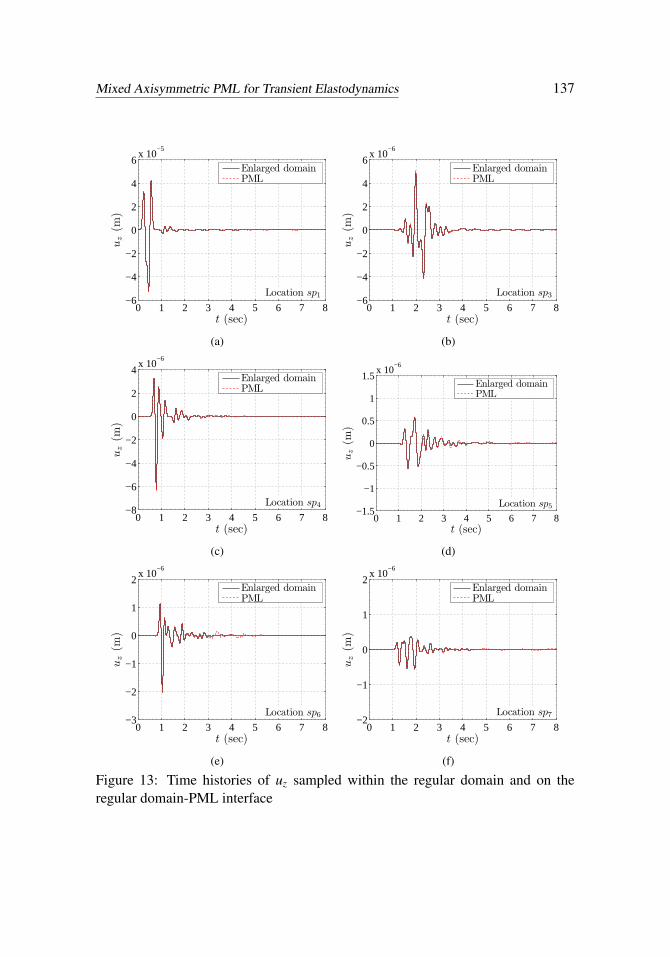
The displacement time histories at the various sampling points were comparedagainst the response obtained using an enlarged domain (40m × 40m). The en-larged domain’s size was defined such that, during the specified time interval ofinterest (8 seconds), reflections from its fixed exterior boundaries do not travelback and interfere with the wave motion in the computational domain of interest.Figure 13 depicts the comparison of the response time histories for uz at various spi
points. As it can be seen the agreement is impressive.
Figure 12: A PML-truncated axisymmetric domain subjected to a stress disk loadon its surface over the region (0m ≤ r ≤ 0.5m)
Figure 14 shows the snapshots of displacement uz taken at two different times (t =0.96s and 1.16s) for both the PML-truncated domain and the enlarged domain (40m× 40m). As before, we mark the PML-interface with dashed lines in the case of theenlarged domain to ease the visual comparison. The agreement is remarkable withno signs of instability or artificial reflections from the interface between the PMLand regular domain. It is interesting to note that the waves are trapped inside thetop layer due to the high-contrast (1 :2) of the material properties of the two layers.The effect of the layer interface is clearly visible in the snapshots at z =−2m .
Next, we quantify the performance of the PML via the error metrics defined ear-lier. Figure 15 depicts the time-dependent displacement norm comparison and thenormalized time-dependent relative error e(t) in percent. The quality of the PMLmanifests itself with a nicely decaying relative error shown in Figure 15(b).
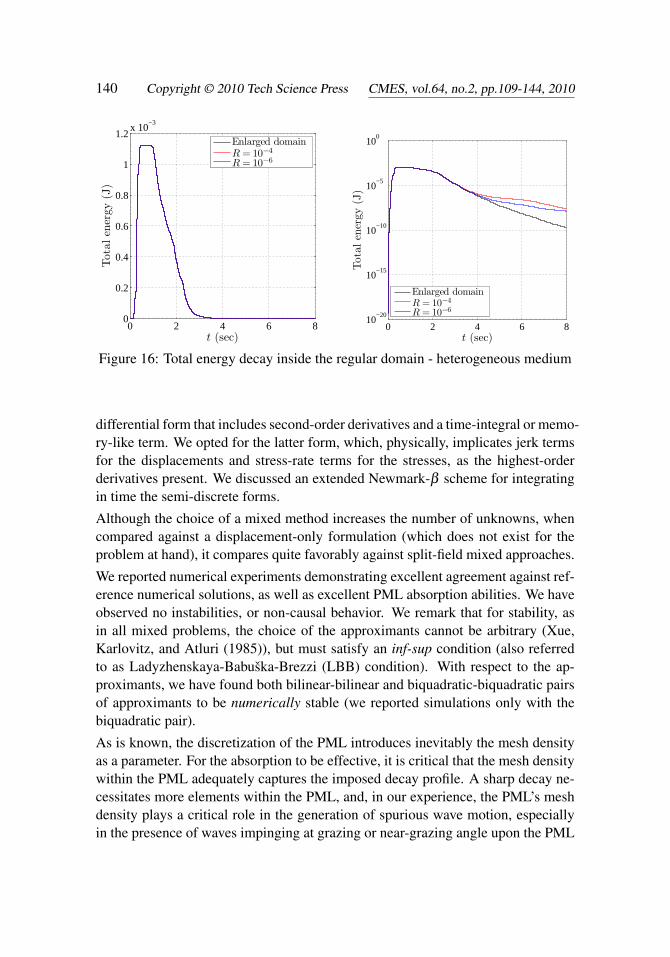
Lastly, Figure 16 depicts the energy decay within the layered medium: in this casethe decay is considerably more gradual than in the homogeneous case, since thereare multiple reflections off of the layer interface that travel back to the free surface,reflect at the free surface, travel downwards to the layer interface, partially reflectthere, travel back to the free surface, and so on and so forth. We explored fourdifferent reflection coefficient values (R = 10−2,10−4,10−6 and R = 10−8). Theobserved behavior is similar to the one discussed in the case of the homogeneoushost: overall, the PML performance is excellent, with no discernible reflections orinstabilities, even in the presence of heterogeneity.
Mixed Axisymmetric PML for Transient Elastodynamics 137
0 1 2 3 4 5 6 7 8−6
−4
−2
0
2
4
6x 10
−5
t (sec)
uz
(m)
Location sp1
Enlarged domainPML
(a)
0 1 2 3 4 5 6 7 8−6
−4
−2
0
2
4
6x 10
−6
t (sec)
uz
(m)
Location sp3
Enlarged domainPML
(b)
0 1 2 3 4 5 6 7 8−8
−6
−4
−2
0
2
4x 10
−6
t (sec)
uz
(m)
Location sp4
Enlarged domainPML
(c)
0 1 2 3 4 5 6 7 8−1.5
−1
−0.5
0
0.5
1
1.5x 10
−6
t (sec)
uz
(m)
Location sp5
Enlarged domainPML
(d)
0 1 2 3 4 5 6 7 8−3
−2
−1
0
1
2x 10
−6
t (sec)
uz
(m)
Location sp6
Enlarged domainPML
(e)
0 1 2 3 4 5 6 7 8−2
−1
0
1
2x 10
−6
t (sec)
uz
(m)
Location sp7
Enlarged domainPML
(f)
Figure 13: Time histories of uz sampled within the regular domain and on theregular domain-PML interface
Figure 14: Comparison of uz snapshots between the PML-truncated (left column)and enlarged (right column) domains - heterogeneous medium
We note that the efficacy of the discussed PML formulation does not depend onthe complexity of the heterogeneity (e.g., multi-layered, non-horizontal layer inter-faces, inclusions, etc). However, here we opted to report results for horizontallylayered media only, since these are the most physically meaningful when axisym-metric geometries are considered.
Finally, we remark that growth of spurious reflections has been reported by otherswhen waves impinge at grazing incidence at the PML-regular domain interface. Ithas also been often reported that the grazing incidence difficulty is associated withthe choice of the classical stretching function, which, by construction, is singularat zero frequency (this has been our choice herein as well). To overcome the sin-
Mixed Axisymmetric PML for Transient Elastodynamics 139
0 1 2 3 4 5 6 7 80
0.4
0.8
1.2x 10
−3
t (sec)
Dis
plac
emen
tfie
ldL
2no
rm
Enlarged domainPML-truncated domain
(a) Displacement field norm D(t;ΩRD)
0 1 2 3 4 5 6 7 80
0.5
1
1.5
2
2.5
3
t (sec)
Nor
mal
ized
L2
erro
r(%
)(b) Relative error e(t)
Figure 15: Error metrics for the heterogeneous domain (Example 2)
gularity, and possibly the perceived difficulty with the grazing angle incidence thathas been attributed to the frequency singularity, modified stretching functions havebeen proposed that are not singular at zero frequency (as discussed in the intro-duction, the CPML is the most notable example of such a development: see, forexample, Martin, Komatitsch, and Gedney (2008)). The CPML has been reportedto alleviate, but not eliminate the growth of spurious reflections (see, for example,the comparisons reported in Meza-Fajardo and Papageorgiou (2008)). To date, allreported studies are purely numerical, and a theoretical proof of the origin of thedifficulty remains elusive. It is not clear whether indeed the origin of the spuriousgrowth at grazing incidence is due to the choice of the stretching function; more-over, careful parameterization of the PML is also capable of alleviating the growth.In this article, we too are not addressing the grazing angle incidence issue, pendingdetailed studies that escape the scope of this communication.
6 Conclusions
We presented the development of a new mixed displacement-stress (or stress his-tory) formulation for forward elastic wave simulations in PML-truncated axisym-metric media. In particular, we used a regularly-stretched, unsplit-field PML, andretained both displacements and stress terms as unknowns to arrive at the mixedscheme. Upon the introduction of approximants, in the Galerkin sense, the re-sulting semi-discrete form can be cast as either third-order in time, or in an integro-
Figure 16: Total energy decay inside the regular domain - heterogeneous medium
differential form that includes second-order derivatives and a time-integral or memo-ry-like term. We opted for the latter form, which, physically, implicates jerk termsfor the displacements and stress-rate terms for the stresses, as the highest-orderderivatives present. We discussed an extended Newmark-β scheme for integratingin time the semi-discrete forms.
Although the choice of a mixed method increases the number of unknowns, whencompared against a displacement-only formulation (which does not exist for theproblem at hand), it compares quite favorably against split-field mixed approaches.
We reported numerical experiments demonstrating excellent agreement against ref-erence numerical solutions, as well as excellent PML absorption abilities. We haveobserved no instabilities, or non-causal behavior. We remark that for stability, asin all mixed problems, the choice of the approximants cannot be arbitrary (Xue,Karlovitz, and Atluri (1985)), but must satisfy an inf-sup condition (also referredto as Ladyzhenskaya-Babuška-Brezzi (LBB) condition). With respect to the ap-proximants, we have found both bilinear-bilinear and biquadratic-biquadratic pairsof approximants to be numerically stable (we reported simulations only with thebiquadratic pair).
As is known, the discretization of the PML introduces inevitably the mesh densityas a parameter. For the absorption to be effective, it is critical that the mesh densitywithin the PML adequately captures the imposed decay profile. A sharp decay ne-cessitates more elements within the PML, and, in our experience, the PML’s meshdensity plays a critical role in the generation of spurious wave motion, especiallyin the presence of waves impinging at grazing or near-grazing angle upon the PML
Mixed Axisymmetric PML for Transient Elastodynamics 141
interface. Although there exists an optimal set of PML parameters (amplitude andpower of decay polynomial) for a given mesh density4, we have found that, in gen-eral, one could expect reasonable performance by using a quadratic profile and areference velocity equal to the average P-wave velocity of the computational do-main.
The extension of the methodology reported herein to the three-dimensional caseis straightforward, and will be reported in future communications. While not ad-dressed herein, the choice of the PML parameters (reference velocity, mesh density,reflection coefficient, etc) is critical in presenting the wave motion with a smoothly-varying decay profile within the PML. A relatively smooth profile is necessary foravoiding spurious reflections that could pollute the solution in the interior. A thor-ough parametric study escapes the scope of the present article, but is necessary forproviding guidance on the parameter choices, and, in turn, for quality solutions.
Acknowledgement: Partial support for this work has been provided by theUS National Science Foundation under grant awards CMMI-0348484 and CMMI-0619078. The authors gratefully acknowledge this support.
References
Arnold, D. N.; Brezzi, F.; Douglas, J. (1984): PEERS: a new mixed finiteelement for plane elasticity. Japan J. Appl. Math, vol. 1, pp. 347–367.
Arnold, D. N.; Brezzi, F.; Fortin, M. (1984): A stable finite element for thestokes equations. Calcolo, vol. 21, pp. 337–344.
Atluri, S. N.; Gallagher, R. H.; Zienkiewicz, O. C. (1983): Hybrid & mixedfinite element methods. J. Wiley & Sons, Chichester.
Basu, U. (2009): Explicit finite element perfectly matched layer for transientthree-dimensional elastic waves. Int. J. Numer. Meth. Engng., vol. 77, pp. 151–176.
Basu, U.; Chopra, A. K. (2003): Perfectly matched layers for time-harmonicelastodynamics of unbounded domains: theory and finite-element implementation.Comput. Methods Appl. Mech. Engrg., vol. 192, pp. 1337–1375.
Basu, U.; Chopra, A. K. (2004): Perfectly matched layers for transient elas-todynamics of unbounded domains. Int. J. Numer. Meth. Engng., vol. 59, pp.1039–1074.
4 There is no simple process that could lead a priori to an optimal set of PML parameters; anoptimization-based process has been reported in Collino and Monk (1998).
Bécache, E.; Fauqueux, S.; Joly, P. (2003): Stability of perfectly matched layers,group velocities and anisotropic waves. Journal of Computational Physics, vol.188, pp. 399–433.
Bécache, E.; Joly, P.; Tsogka, C. (2001): Fictitious domains, mixed finite ele-ments and perfectly matched layers for 2D elastic wave propagation. J. Comput.Acoust., vol. 9, no. 3, pp. 1175–1202.
Bérenger, J.-P. (1994): A perfectly matched layer for the absorption of electro-magnetic waves. Journal of Computational Physics, vol. 114, pp. 185–200.
Bérenger, J.-P. (2002): Application of the CFS PML to the absorption of evanes-cent waves in waveguides. IEEE Microwave and Wireless Components Letters,vol. 12, no. 6, pp. 218–220.
Bérenger, J.-P. (2002): Numerical reflection from FDTD-PMLs: a comparisonof the split PML with the unsplit and CFS PMLs. IEEE Transactions on Antennasand Propagation, vol. 50, no. 3, pp. 258–265.
Brezzi, F. (1988): A survey of mixed finite element method. In Dwoyer, D.;Hussaini, M.; Voigt, R.(Eds): Finite Elements Theory and Application, pp. 34–49,New York. Springer-Verlag.
Brezzi, F.; Douglas, J.; Marini, L. D. (1985): Two families of mixed finiteelement methods for second order elliptic problems. Numer. Math., vol. 47, pp.217–235.
Chew, W. C.; Jin, J. M.; Michielssen, E. (1997): Complex coordinate systemas a generalized absorbing boundary condition. In Proc. 13th Annu. Rev. of Prog.Appl. Comp. Electromag., pp. 909–914, Monterey,CA. Vol. 2.
Chew, W. C.; Liu, Q. H. (1996): Perfectly matched layers for elastodynamics:a new absorbing boundary condition. Journal of Computational Acoustics, vol. 4,no. 4, pp. 341–359.
Chew, W. C.; Weedon, W. H. (1994): A 3D perfectly matched medium frommodified Maxwell’s equations with stretched coordinates. Micro. Opt. Tech. Lett.,vol. 7, pp. 599–604.
Cohen, G.; Fauqueux, S. (2005): Mixed spectral finite elements for the linearelasticity system in unbounded domains. SIAM J. Sci. Comput., vol. 26, no. 3, pp.864–884.
Collino, F.; Monk, P. B. (1998): Optimizing the perfectly matched layer. Comput.Methods Appl. Mech. Engrg., vol. 164, pp. 157–171.
Mixed Axisymmetric PML for Transient Elastodynamics 143
Collino, F.; Tsogka, C. (2001): Application of the perfectly matched absorb-ing layer model to the linear elastodynamic problem in anisotropic heterogeneousmedia. Geophysics, vol. 66, no. 1, pp. 294–307.
Drossaert, F. H.; Giannopoulos, A. (2007): Complex frequency shifted convo-lution PML for FDTD modelling of elastic waves. Wave Motion, vol. 44, no. 7-8,pp. 593–604.
Drossaert, F. H.; Giannopoulos, A. (2007): A nonsplit complex frequency-shifted PML based on recursive integration for FDTD modeling of elastic waves.Geophysics, vol. 72, no. 2, pp. T9–T17.
Farrell, C.; Leonhardt, U. (2005): The perfectly matched layer in numericalsimulations of nonlinear and matter waves. Journal of Optics B: Quantum andSemiclassical Optics, vol. 7, pp. 1–4.
Festa, G.; Nielsen, S. (2003): PML absorbing boundaries. Bulletin of theSeismological Society of America, vol. 93, no. 2, pp. 891–903.
Festa, G.; Vilotte, J.-P. (2005): The Newmark scheme as velocity-stress time-staggering: an efficient PML implementation for spectral element simulations ofelastodynamics. Geophys. J. Int., vol. 161, pp. 789–812.
Gedney, S. D. (1996): An anisotropic perfectly matched layer-absorbing mediumfor the truncation of FDTD lattices. IEEE Transactions on Antennas and Propa-gation, vol. 44, no. 12, pp. 1630–1639.
Harari, I.; Albocher, U. (2006): Studies of FE/PML for exterior problems oftime-harmonic elastic waves. Comput. Methods Appl. Mech. Engrg., vol. 195, pp.3854–3879.
Hastings, F. D.; Schneider, J. B.; Broschat, S. L. (1996): Application of theperfectly matched layer (PML) absorbing boundary condition to elastic wave prop-agation. J. Acoust. Soc. Am., vol. 100, no. 5, pp. 3061–3069.
Hu, F. Q. (1996): On absorbing boundary conditions for linearized Euler equa-tions by a perfectly matched layer. Journal of Computational Physics, vol. 129,pp. 201–219.
Johnson, C.; Mercier, B. (1978): Some equilibrium finite element methods fortwo-dimensional elasticity problems. Numer. Math., vol. 30, pp. 103–116.
Komatitsch, D.; Martin, R. (2007): An unsplit convolutional perfectly matchedlayer improved at grazing incidence for the seismic wave equation. Geophysics,vol. 72, no. 5, pp. SM155–SM167.
Komatitsch, D.; Tromp, J. (2003): A perfectly matched layer absorbing bound-ary condition for the second-order seismic wave equation. Geophysical JournalInternational, vol. 154, pp. 146–153.
Kuzuoglu, M.; Mittra, R. (1996): Frequency dependence of the constitutiveparameters of causal perfectly matched anisotropic absorbers. IEEE Microwaveand Guided Wave Letters, vol. 6, no. 12, pp. 447–449.
Liu, Q. H. (1999): Perfectly matched layers for elastic waves in cylindrical andspherical coordinates. J. Acoust. Soc. Am., vol. 105, no. 4, pp. 2075–2084.
Liu, Q. H.; He, J. Q. (1998): Quasi-PML for waves in cylindrical coordinates.Microwave and Optical Technology Letters, vol. 19, no. 2, pp. 107–111.
Liu, Q. H.; Sinha, B. K. (2003): A 3D cylindrical PML/FDTD method forelastic waves in fluid-filled pressurized boreholes in triaxially stressed formations.Geophysics, vol. 68, no. 5, pp. 1731–1743.
Martin, R.; Komatitsch, D.; Gedney, S. (2008): A variational formulationof a stabilized unsplit convolutional perfectly matched layer for the isotropic oranisotropic seismic wave equation. CMES: Computer Modeling in Engineering &Sciences, vol. 37, no. 3, pp. 274–304.
Meza-Fajardo, K. C.; Papageorgiou, A. S. (2008): A nonconvolutional, split-field, perfectly matched layer for wave propagation in isotropic and anisotropicelastic media: Stability analysis. Bulletin of the Seismological Society of America,vol. 98, no. 4, pp. 1811–1836.
Raviart, P. A.; Thomas, J. M. (1977): A mixed finite element method for secondorder elliptic problems. In Galligani, I.; Magenes, E.(Eds): Mathematical Aspectsof the Finite Element Method, Lecture Notes in Mathematics, volume 606, pp. 292–315, New York. Springer-Verlag.
Roden, J. A.; Gedney, S. D. (2000): Convolutional PML (CPML): an efficientFDTD implementation of the CFS-PML for arbitrary media. Microwave and Op-tical Technology Letters, vol. 27, no. 5, pp. 334–339.
Roden, J. A.; Gedney, S. D. (2000): An efficient FDTD implementation ofthe PML with CFS in general media. IEEE Antennas and Propagation SocietyInternational Symposium, vol. 3, pp. 1362–1265.
Teixeira, F. L.; Chew, W. C. (1997): Perfectly matched layer in cylindrical co-ordinates. In Antennas and Propagation Society International Symposium Digest,pp. 1908–1911, Montreal, Canada. IEEE. Vol. 3.
Teixeira, F. L.; Chew, W. C. (1997): PML-FDTD in cylindrical and sphericalgrids. IEEE Microwave and Guided Wave Letters, vol. 7, no. 9, pp. 285–287.
Mixed Axisymmetric PML for Transient Elastodynamics 145
Teixeira, F. L.; Chew, W. C. (1997): Systematic derivation of anisotropic PMLabsorbing media in cylindrical and spherical coordinates. IEEE Microwave andGuided Wave Letters, vol. 7, no. 11, pp. 371–373.
Teixeira, F. L.; Chew, W. C. (1999): On causality and dynamic stability ofperfectly matched layers for FDTD simulations. IEEE Transactions on MicrowaveTheory and Techniques, vol. 47, no. 6, pp. 775–785.
Teixeira, F. L.; Chew, W. C. (2000): Complex space approach to perfectlymatched layers: a review and some new developments. Int. J. Numer. Model., vol.13, pp. 441–455.
Tsynkov, S. V. (1998): Numerical solution of problems on unbounded domains. areview. Appl. Numer. Math., vol. 27, no. 4, pp. 465–532.
Turkel, E.; Yefet, A. (1998): Absorbing PML boundary layers for wave-likeequations. Applied Numerical Mathematics, vol. 27, pp. 533–557.
Wang, J.; Wang, Y.; Zhang, D. (2006): Truncation of open boundaries ofcylindrical waveguides in 2.5-dimensional problems by using the convolutionalperfectly matched layer. IEEE Transactions on Plasma Science, vol. 34, no. 3,pp. 681–690.
Xue, W.-M.; Karlovitz, L. A.; Atluri, S. N. (1985): On the existence and stabilityconditions for mixed-hybrid finite element solutions based on reissner’s variationalprinciple. J. of Solids and Structures, vol. 21, no. 1, pp. 97–116.
Zampolli, M.; Tesei, A.; Jensen, F. B. (2007): A computationally efficient finiteelement model with perfectly matched layers applied to scattering from axiallysymmetric objects. J. Acoust. Soc. Am., vol. 122, no. 3, pp. 1472–1485.
Zeng, Y.; He, J. Q.; Liu, Q. H. (2001): The application of the perfectly matchedlayer in numerical modeling of wave propagation in poroelastic media. Geo-physics, vol. 66, no. 4, pp. 1258–1266.
Zhao, L. (2000): The generalized theory of perfectly matched layers (GT-PML)in curvilinear co-ordinates. Int. J. Numer. Model., vol. 13, pp. 457–469.


![PropellersPropellers - Honda · PDF file01/2012 [D]3.a • Replacement propeller for BF2D ~ BF2.3D • Perfectly matched to ensure optimum performance Plastic Propeller (3 Blade)](https://static.documents.pub/doc/80x56/5a75e06e7f8b9a9c548ce157/propellerspropellers-honda-marine-012012-d3a-replacement-propeller.jpg)


