A MODEL FOR FLUID FLOW BETWEEN PARALLEL, CO-ROTATING ...

A MODEL FOR FLUID FLOW BETWEEN

PARALLEL, CO-ROTATING

ANNULAR DISKS

ThesisSubmitted to

Graduate Engineering and ResearchSchool of Engineering

UNIVERSITY OF DAYTON

In Partial Fulfillment of the Requirements forThe Degree

Master of Science in Mechanical Engineering

byefFrey Stuart Allen

University of DaytonDayton, Ohio

July, 1990

A MODEL FOR FLUID FLOW BETWEENPARALLEL, CO-ROTATING ANNUALAR DISKS

Approved by:

Kevin Hallinan, Ph.D.Advisory Committee, Chairman

/Z’Gary A. Th’iele, PhD.Associate Dean/DirectorGraduate Engineering and ResearchSchool of Engineering

Gordon A. Sargent, Ph.D.Dean, School of Engineering

Acknowledgements

I am deeply indebted to my family, friends, and associates for their support dur

ing the course of this work and my education. In particular, I would like to thank

Dr. John Schauer for getting me started on this project and for his continual guid

ance and support. And I greatly appreciate the faculty and staff of the mechanical

engineering department for their assistance and patience. I would also like to thank

Dr. Costandy Saba and Dr. Vinod Jam for providing me with the financial means to

pursue my master studies. An enormous debt of gratitude goes to my good friend

Frank Lung for his technical assistance and for his help in preparing this thesis. I

can not thank enough Dr. Kevin Hallinan who inherited the role of my thesis advisor.

Without his considerable time and effort I would have never finished. Finally, I would

especially thank my parents, Bryant and Carol, for their patience, understanding, and

support; to them I dedicate this work.

111

Abstract

A MODEL FOR FLUID FLOW BETWEENPARALLEL, CO-ROTATING ANNULAR DISKS

Allen, Jeffrey StuartUniversity of Dayton, 1990Advisor: Dr. Kevin Hallinan

A model for fluid flow between parallel, co-rotating annular disks is developedfrom conservation of mass and conservation of momentum principles. Through theassumption of fully-developed boundary layer flow a closed form solution is found forthe velocity components and the pressure. These solutions are then applied to theconservation of angular momentum principle from which a closed form solution forthe torque of the system is found.

The model can be used to analyze the fluid/disk system in either a pump ora turbine configuration. The only change necessary is a slight modification of theboundary conditions. The accuracy of the results in both cases improves as thedimensionless parameter R* increases. An R* on the order of or greater than 1indicates that viscous effects are important and the model appears to be very accuratein this range.

Other dimensionless parameters similar to R* appear in the development whichalso describe various aspects of the model. These parameters are discussed with respect to the force effects (momentum, Coriolis, centripetal, viscous, and pressure)that each describe. In addition, the performance of a turbine configuration is investigated with the model and the moment of momentum relationship developed fromthe model.

The results of this analysis appear to be promising for describing rotating viscousflows and justify further investigation.

Contents

Table of Contents vList of Figures viiiList of Tables ixNomenclature x

1 INTRODUCTION 11.1 Background 1

1.1.1 History 31.1.2 Model Geometry 3

1.2 Scope of Work 6

2 ANALYTICAL MODEL 92.1 Differential Equations of Motion 102.2 Velocity Profile 122.3 Solution to Continuity 152.4 The R—Constant 162.5 Solution to Momentum Equations 182.6 Summary 20

3 BOUNDARY CONDITIONS 213.1 Mass Flow Rate and Angular Velocity 213.2 Tangential Velocity and Angle of Tangency 24

4 CHARACTERISTICS PARAMETERS 284.1 Dimensionless Parameters y and Re6 294.2 .1? 294.3 Angular Velocity Constant, c 314.4 Rossby Number 324.5 Summary 33

5 PATHLINES5.1 Change In Angular Position of Fluid5.2 Pathlines And Relative Velocities 38

6 TORQUE AND POWER6.1 Conservation of Angular Momentum6.2 Torque6.3 Power

7 RESULTS AND DISCUSSION7.1 Model Verification7.2 System Performance7.3 Model Behavior7.4 Summary

8 CONCLUSION8.1 Summary of Model8.2 Recommendations

A Conservation of MassA.1 Reduction of ContinuityA.2 Solution for the Radial Velocity Component

B.3 Incorporating ContinuityB.3.1 r-momentumB.3.2 9-momentum

B.4 7 VS. Re6B.5 The R ConstantB.6 Summary

68

6871727373757777

79

808284

D Solution to r-MomentumD.1 IntegrationsD.2 Solution

8692

3535

41414447

4848505360

616162

656566

B Conservation of MomentumB.1 Reduction of the Navier-Stokes EquationsB.2 Velocity Profile Function

C Solution to 0-MomentumC.1 Homogeneous SolutionC.2 Particular SolutionC.3 Total Solution

85

E Conservation of Angular Momentum 94E.1 Rotating Control Volume . . . 94E.2 Conservation of Angular Momentum . . . . . . 97E.3 Solution to Moment of Momentum . . . . . . . 100

E.3.1 Surface Integral Evaluation . . . . . .. 103

E.3.2 Volume Integral Evaluation . . . . . .. 105

F Program Listing 108

G Data Files 129

vii

List of Figures

1.1 Basic Rotor Construction for System 21.2 Geometry of Model for Rotor 51.3 Fluid Element: Orientation, Forces, and Velocities 7

3.1 Directions of the Radial Velocity Component 233.2 Angle of Tangency 26

5.1 Incremental Change in Fluid Particle Position 375.2 Typical Pathline For Turbine Configuration 39

6.1 Control Volume Definition for System Model (N = 0) 43

7.1 Torque versus Angular Velocity for Various 6 517.2 Power versus Angular Velocity for Various S 547.3 Normalized Pressure for Various R 557.4 Pathlines for Various R* 577.5 R versus r* 587.6 V versus r* 59

E. 1 Rotating Control Volume Relative to Inertial Frame of Reference . . 95E.2 Control Volume Definition 102

viii

List of Tables

1.1 Coordinate and Velocity Components 4

1.2 Specifying Parameters for Rotor 6

2.1 )L—Coefficient Values 14

3.1 Determination of System Constants 27

7.1 System Specification for Figures 7.1 and 7.2 50

B.1 Typical Rotor and Fluid Parameters for Turbine Configuration . 76

D.1 Values of Functions Fm and Gm for Various m 89

ix

Nomenclature

Variables Functions

A cross-sectional area .F() velocity profile functiona constant for U(r) Fm,Gm factorial functionsb constant for (r) Sm(r) series functionc constant for V(r) V gradient functiond constant for P t incremental changeê unit vectorg body forcegc gravitational constant Subscriptshp horsepower

mass flow rate CAL. control volumem,n series indices i inner radiusN number of disks on rotor j vector indiceF pressure m series function indicatorP power o outer radiusr radial position r radial, or based on radiusR system constant z axialR Reynold’s number 6 based on half-disk spacingT torque 0 tangential

u,U radial velocityv,V absolute tangential velocity15 ,V relative tangential velocity Superscripts

,L volumew axial velocity dimensionlessz axial position

a angle of tangencyaspect ratio

S half-disk spacing,i axial position, z/SO angular postionw angular velocity of rotor

angular velocity of fluidA velocity profile constant

Chapter 1

INTRODUCTION

1.1 Background

The system under study consists of fluid flowing between parallel, co-rotating annular

disks. The rotor, or rotating assemblage, of the system is constructed by attaching

a stack of annular disks to a central shaft. Figure 1 illustrates the basic rotor con

figuration. This fluid-rotor system can operate either as a pump or as a turbine. In

both instances energy transfer between the fluid and the rotor occurs through viscous

effects. The operation of this system, as either as a pump or as a turbine, utilizes

shear stresses in the fluid at the disk face which are created by a velocity differen

tial between the fluid and the rotor. In the pump configuration, the velocity of the

disks at a given radius is greater than the tangential velocity of the fluid at that

radius; therefore, kinetic energy is transferred from the rotor to the fluid through vis

cous interaction at the disk face. In the turbine configuration, the disks are rotating

slower than the tangential velocity of the fluid for a given radius and kinetic energy

is transferred from the fluid to the rotor.

CHAPTER 1. INTRODUCTION

Figure 1.1: Basic Rotor Construction for System

CHAPTER 1. INTRODUCTION 3

1.1.1 History

The system under investigation in this study was first introduced in 1911 by Nikola

Tesla as a turbine. In 1913 he demonstrated the concept with a steam powered, eight

inch diameter turbine that developed over 200 horsepower[1,2]. A patent was issued

to Tesla for both the concept and the device[3,4], hence the name Tesla Turbine. The

turbine configuration is also referred to as the shear-torque turbine and the bladeless

turbine. Since Tesla’s original work the turbine has been more of a curiosity of

acadamia than a practical device; although it has been developed for use in dentist

drills. Some other applications that have been considered involve small propulsive

devices for expendable weapons, such as torpedoes[5].

The pump configuration has been developed much more extensively both practi

cally and analytically. This attention results from the long operating life this type of

pump would exihibit in harsh environments. With a no-slip condition at the fluid—disk

interface there would be less wear on components than found in typical pumps which

rely upon direct momentum exchange for inducing fluid motion. In other words, with

a typical pump the fluid impinges upon the rotor and this impingement accelerates

rotor wear; whereas, the pump configuration of the system under study does not have

this collision between the fluid and the rotor. This style of pump has been com

mercially developed for slurries or fluids containing solid objects that would damage

either conventional pumps or the objects being pumped. One such application is

in fisheries where this type of pump allows fish and rocks to pass through without

damage to the pump or fish.

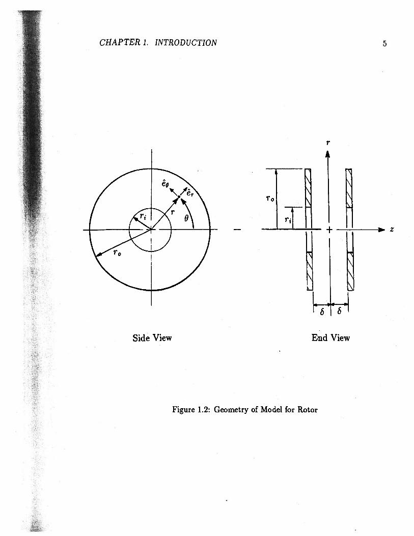
1.1.2 Model Geometry

Studying the performance of the device shown in Figure 1.1 requires that the inter

action between the fluid and the rotor be modelled. In general, when the interaction


Table 1.1: Coordinate and Velocity Components

Coordinate Component Velocityradial: r u

tangential: 6 vaxial: z w

between the fluid and the rotor is being discussed the term system will be used. Whenthe operation of this device, as a pump or as a turbine, is being discussed the termconfiguration will be used. The term model refers to the application of the equationsof motion to the two-disk system shown in Figure 1.2. The model can be used ineither a turbine configuration or a pump configuration.

Figure 1.2 illustrates the geometry of the rotor. A cylindrical coordinate systemwhere the z-axis coincides with the axis of rotation. The notation used for coordinatesand velocities is shown in Table 1.1.

Figure 1.2 illustrates the model geometry of the rotor. A single pair of disks willbe used to model the fluid-disk interface; for actual rotors the model results will bemultiplied by a coefficient corresponding to the number of disk pairs on the rotor:

ROTORc1= C(# of disks) * ROTORmodel.

If the disk faces are parallel to one another and the distance between the disksis constant over the radius of the rotor, then four parameters will completely specify the rotor geometry. These four parameters are outer radius, inner radius, diskspacing, and the number of disks. Table 1.2 defines the nomenclature used for theseparameters. The coefficient corresponding to the number of disks, N, is defined suchthat for a single pair of disks (the model geometry) N is equal to zero:

C(#ofdisks)=N+1.


r

e/

‘bill

Side View End View

Figure 1.2: Geometry of Model for Rotor


Table 1.2: Specifying Parameters for Rotor

Outer Radius: r0Inner Radius: r:

Half—Disk Spacing:Number of Disks: N

Therefore, the performance of ROTORuaj must equal the ROTOR,,ej perfor

mance for a system having only two disks.

Figure 1.3 illustrates the shear stresses on a fluid element in the turbine corifigu

ration. The shear stress in the radial direction is defined as r7 and the shear stress

in the tangential direction is defined as Tt. The shear stresses arise from the velocity

differential between the fluid and rotor and are the primary source of energy transfer

for this system. This study focuses on finding the velocity differential responsible for

the shear stresses.

1.2 Scope of Work

The goal of this study is to develop a procedure to predict the exchange in energy

between the fluid and the rotor for various fluid properties, rotor configurations, and

operating conditions. With the energy transfer known, the performance of the system

as either a pump or a turbine can be calculated. The procedure will be to determine

the velocity components of the fluid relative to the rotor and then to calculate the

torque resulting from the sum of the shear forces across the disk faces.

The emphasis of this study is on the development of a new model and not on

the use of the model. Several different rotor configurations and system operating

conditions are studied, but even the study of these few systems is far from complete.

The use of the model is concentrated on gaseous fluids in a turbine configuration since


Figure 1.3: Fluid Element: Orientation, Forces, and Velocities

suo4puo£iptrnoqaqrnare£aesso3usuetp

£pioatjjs!suuqinaoJStSstsJtreduindJoJP!JspadopApPPOW

‘11“°HiiUtRLuis 4CsS!tI$U!‘W!IeU!!10

NOLLDflcfOLLNIr?J2LLJVHO

Chapter 2

ANALYTICAL MODEL

This chapter highlights the model development detailed in Appendix A through D

and discusses various properties of the model and the behavior of specific terms

contained within the model equations. The analytical model will be developed from

general conservation principles; i.e. mass, momentum, and energy. The purpose

of this model is to predict fluid velocity components and pressures for various fluid

properties, rotor configurations, and operating conditions. In other words, given a

description of the system the analytical model will describe the behavior of the fluid

within the system. Once the velocity components are known the performance of the

system, either as a pump or turbine, can be determined.

The complete development of the analytical model is contained in Appendix A

through Appendix D. Appendix A describes the reduction of the continuity equation

and the solution for the radial velocity component of the fluid. Appenix B describes

the reduction of the momentum equations. In Appendix C the 0-momentum equation

is solved for the relative tangential velocity component, c. The pressure is found by

solving the r-momentum equation and is shown in Appendix D.

CHAPTER 2. ANALYTICAL MODEL 10

2.1 Differential Equations of Motion

Several approximations are imposed upon the general conservation principles in thedevelopment of the fluid model. The first approximation is isentropic flow. Sincethe temperature is constant throughout the flow there is no exchange in thermalenergy and the conservation of energy principle need not be used. Therefore, the fluidmodel may be described by thç differential forms of the conservation of mass and theconservation of momentum principles only. Expressed vectorially these principles are:

Conservation of Mass:

(2.1)

Conservation of Momentum:

. / — — — — -. 2-.u + u. V,j u = —VP + g + i’V u. (2.2)

Further approximations are applied to the mass and momentum conservation principles; such as incompressibility of the fluid which, with the assumption of isentropicflow, uncouples the governing Equations 2.1 and 2.2. Also, the flow is assumed tobe steady-state, and body forces are ignored. Another assumption is that of fully-developed boundary layer flow existing throughout the rotor. This is the worst assumption of the model and the appropriateness of this assumption will be discussedlater. Assuming fully-developed flow does, however, eliminate axial flow between thedisks. That is, the axial component, w, of the fluid velocity is zero. Therefore, thecharacteristics of the fluid velocity field, i, may be modelled using a velocity profilenormal to the boundary layer; i.e., in the axial direction. Using a velocity profile forthe flow effectively makes the field one-dimesional; however, the conservation equations are two dimensional in the coordinate system defined for the model shown inFigure 1.2. With these assumptions the conservation equations may now used to solvefor two components of the velocity and pressure (r and 9) at the centerline (z = 0)


of the model.

The velocity profile exists only for those components of the velocity relative to the

rotating disk face. But the conservation equations are only valid for velocities relative

to a non-rotating frame of reference. Therefore, to use the velocity profile in the

conservation equations the absolute velocities are referenced to the rotating coordinate

system. For the absolute radial velocity componenet, u, there is no change; the disk

surface is not moving relative to r. However, the tangential velocity component, v,

does change between rotating and stationary frames of reference. If we define v as

the tangential velocity component of the fluid relative to a fixed frame of reference

and € as the tangential velocity component relative to a rotating frame of reference;

i.e. the disk face, then the absolute tangential velocity, v, is a function of 3 such that•

v(r, 9) = f3(r, 9) + rw (2.3)

where w is the angular velocity of the rotor. The tangential velocity component

relative to the disk face, i3, will be referred to as the relative tangential velocity

throughout the rest of this study. By substituting Equation 2.3 into the conservation

relations (Equations 2.1 and 2.2) for v we can use the velocity proffle in modelling

the flow field. This transformation also introduces Coriolis and centripetal forces into

the convective term, (ii. ‘)ii, of the the conservation of momentum, Equation 2.2.

Now, assume that the flow characterisitics are independent of the angular position.

In other words, the velocity and pressure components are constant with respect to 0.

This assumption will have repurcussions in defininng the boundary conditions, later.

For nozzle directed flow in a turbine this assumption is not very precise. However,

for a pump this is generally an accurate estimate of the flow conditions. The velocity

components can now be expressed as the product of a radially dependent function at

z = 0 and a velocity profile function.

Applying these approximations to the conservation principles we can reduce Equa


tions 2.1 and 2.2 to the following forms:

continuity:ö(ru)

= 0, (2.4)

r—momentum:

I a i522 ldP (82u lOu u\

— (2gw) — (rw) = ——— + vI—+————I + vI—I\ Or rj p dr Or r Or r2 J \ t9z2j

(2.5)

8—momentum:

I 8€’ u€’\ (82,5 1O5 iY\ fOfi\

+ —) + (2uw) = ii + — — + V -j) (2.6)

2.2 Velocity Profile

If we define i = z/6 and the velocity proffle function as F(r1) then the velocity’

components of Equations 2.5 and 2.6 become

u(r,8) = U(r).F() (2.7)

and

ii(r,O) = c’(r)F(q) (2.8)

where U(r) and 7(r) are the centerline values (z = 0) of u and €3, respectively. The

seperation of variables for the velocities, u and €3, is possible through the assumption

of fully-developed boundary layer flow. Substituting the product function form of the

velocity components, Equations 2.7 and 2.8, into Equations 2.4, 2.5, and 2.6 produces

the following form of the differential equations of motion:


continuity:ld(rU)

— 0 29r dr —

r—momentum:

F2(i) (u—

— F(1) (2’w) — (rw2) =

—ldP Id2U ldU U’ vUPF(i7)d + ‘Th)lj2+d 2) + 52 dir72

‘ (2.10)

0—momentum:

F2(i) (uç+

+ FOi) (2Uw) =

I&V ldV 17\ rd2.F(,l)v.F(i) +

— + di72(2.11)

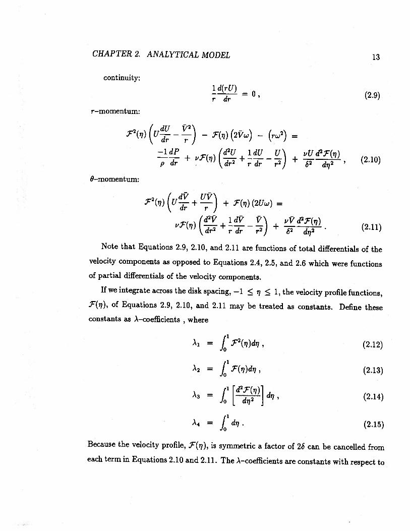
Note that Equations 2.9, 2.10, and 2.11 are functions of total differentials of thevelocity components as opposed to Equations 2.4, 2.5, and 2.6 which were functionsof partial differentials of the velocity components.

If we integrate across the disk spacing, —1 ‘i 1, the velocity profile functions,of Equations 2.9, 2.10, and 2.11 may be treated as constants. Define these

constants as A—coefficients , where

= £1F2(i7)dir1, (2.12)

A2 = j.F(i)d?, (2.13)

I d2F()= J [ drj2 ] dii (2.14)

A4= j

d,7. (2.15)

Because the velocity profile, is symmetric a factor of 25 can be cancelled from

each term in Equations 2.10 and 2.11. The A—coefficients are constants with respect to


Table 2.1: A—Coefficient Values

Laminar TurbulentA 8/15 7/9A2 2/3 7/8A3 —2 1/0: undefined

r; therefore, the characteristics of Equations 2.9, 2.10, and 2.11 remain unchanged for

different flow regimes. The behavior of these equations for a laminar velocity profile

is the same as for a turbulent velocity profile; only the value of the A—coefficients vary.

Let us examine the A—coefficients for two profiles. A power law is used to approx

imate a turbulent velocity profile:

= (1 — ,)1/7 (2.16)

and a laminar velocity profile is approximated as parabolic:

(2.17)

By substituting Equations 2.16 and 2.17 into Equations 2.12, 2.13, and 2.14 we can

compute the values of A1, A2, and A3. The comparison is shown in Table 2.1

In Table 2.1 we see that the convective coefficients, A1 and A2, approach 1 as

the flow becomes turbulent. This is due to A1 and A2 being the averages of the

convective effects in the velocity field. For instance, in slug flow both A1 and A2

would equal 1. TheA3—coefflcient acts on the viscous dissipation terms and is a

measure of the strain rate of the fluid at the wall. Unfortunately, the derivative

of the turbulent power law approximation, Equation 2.16, breaks down at the wall

= ±1) and results in an undefinedA3—coefficient. Therefore, some other measure

of the strain rate at the disk face, such as a Blausius relation, must be used to

determine A3. The power law approximation is, however, still valid for A1 and A2.


This study concentrates on the general behavior of fluid flow in parallel co-rotatingannular disks; subsequently, the exact values of the A—coefficients are not crucial. For

the purposes of this study the A—coefficients corresponding to a parabolic velocity

profile (laminar flow), Equation 2.17, will be used.

Now, substitute the A—coefficients into Equations 2.9, 2.10, and 2.11. A factor of26 is cancelled from each term. The equations of motion become;

continuity:

+ =0 (2.18)

r—momentum:

I dU V2’\ I’/ 2

— A22Vw) — rw =dr rj-ldP f&U ldU U’\ vU

+ A2v I —i- + ———- I + A3— (2.19)p dr \dr rdr rj 32

0—momentum:

+ A2(2Uu) = A2v(_+ “_)

+ A3!. (2.20)

2.3 Solution to Continuity

Examining Equation 2.18 we find that the radial velocity component at the centerline, U(r), is independent of the flow regime since there is no dependency uponthe A—coefficients. Thus, the radial velocity relationship is identical for laminar andturbulent flows. Solving Equation 2.18 (See Appendix A) for the radial velocity component results in:

U(r) = , (2.21)

where a is an undetermined constant dependent upon the boundary conditions. InEquation 2.21 we see that the radial velocity component is directly proportional tothe inverse of radial position; as the radius decreases the radial velocity increases.


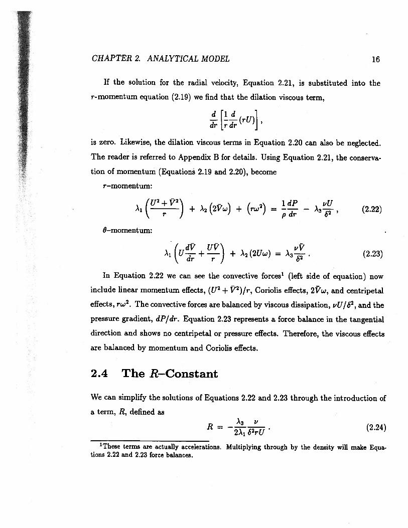
If the solution for the radial velocity, Equation 2.21, is substituted into the

r-momentum equation (2.19) we find that the dilation viscous term,

d ld-1(rU)

is zero. Likewise, the dilation viscous terms in Equation 2.20 can also be neglected.

The reader is referred to Appendix B for details. Using Equation 2.21, the conserva

tion of momentum (Equations 2.19 and 2.20), become

r—momentum:

(U2 + 172)

+ A2 (217w) + (rw2) =— A3--, (2.22)

0—momentum:

(u+) + A2 (2Uw) = (2.23)

In Equation 2.22 we can see the convective forces1 (left side of equation) now

include linear momentum effects, (U2 + 172)/r, Coriolis effects, 2Vw, and centripetal

effects, rw2. The convective forces are balanced by viscous dissipation, vU/62,and the

pressure gradient, dP/dr. Equation 2.23 represents a force balance in the tangential

direction and shows no centripetal or pressure effects. Therefore, the viscous effects

are balanced by momentum and Coriolis effects.

2.4 The R—Constant

We can simplify the solutions of Equations 2.22 and 2.23 through the introduction of

a term, R, defined as

R= )j152u (2.24)

1These terms are actually accelerations. Multiplying through by the density will make Equations 2.22 and 2.23 force balances.


Note that the units for Equation 2.24 are [1/length2]. Therefore, we can define a

dimensionless term, R*, such that

R = Rr2. (2.25)

Now, if we define the aspect ratio of the rotor, r/6, as ‘y, Equation 2.25 can be

rearranged asA ,.,2

———----—— 226

— 2A1Re,.

or

R— 227— 2A1Re8

where Re,. is the radial Reynold’s number:

Re,. = = (2.28)

and Re5 is the Reynold’s number based upon disk spacing:

Re5 = (2.29)

Therefore, R is a ratio of the rotor configuration to the viscous/momentum force

balance. Also, the radial Reynold’s number, Re,., is a constant for the system while

Re5 is dependent upon radial position.

Using the definition of R, Equation 2.24, we can rearrange the momentum equa

tions, 2.22 and 2.23, to

r—momentum:

= A1(U2 + 2)

+ A2 (2iw) + (rw2) +. A3 (!.cL), (2.30)

0-momentum:

+ (1+2Rr2)r + = 0. (2.31)


We found that the radial velocity component, U, could be solved explicitely fromcontinuity, Equation 2.18. From Equations 2.30 and 2.31 we see that the relative tangential velocity, V, can be explicitely solved from the conservation of 0—momentum,Equation 2.31, and the pressure can be explicitely solved for from Equation 2.30.

2.5 Solution to Momentum Equations

The solution for Equation 2.31 (See Appendix C) results in a power series expressionfor the relative tangential velocity:

c’(r)= bSm(R”) — c

(2.32)

where Sm(f) is a power series function of r,

Sm(R) = (—‘f).(2.33)

m=O m.

In Equation 2.32 the constant, b, is dependent upon the boundary conditions. Thesecond constant, c, is a function of angular velocity, w, and R:

c = !(). (2.34)

The solution for the pressure is obtained by substituting the expressions for the radial and relative tangential velocities, Equations 2.21 and 2.32, into the r—momentumrelation, Equation 2.30, and integrating with respect to r (See Appndix D). The solution for the pressure was simplified through the introduction of a convention forfactorial functions:

Fm = , (2.35)

and

Gm=0(m—n)!

= FnFm..n. (2.36)

Using these conventions the solution for the pressure becomes:


1P(r) =— { [a + (b — c)2]

1}

_Ai{(b2_2bc)Rlnr2} II00 R m+1

—{bR

O

[bGm2— 2CFm+21} III

—A1 {(c2— bc) Rlnr2} Iv

00 m+1

—A1 {bR,m . 1)

[_2CFm+i]}

+ {[w2]}. vi

_Ai{(a2)Rlnr2} VII

+ d (2.37)

The terms on the right side of Equation 2.37 are seperated with respect to the type

of force effect from which each term evolved. For example, the integration of the

convective term in Equation 2.30 results in terms I, II, and III. Summarizing the

grouping:

• I, II, and III are from convective effects, (U2 + f72) /r

• IV and V are from Coriolis effects, 2Vw

• VI is from centripetal effects, rw2

• VII is from viscous effects, (vU) /62

• d is an unknown constant of integration.


If we rearrange Equation 2.37 so as to group the terms by like powers of r a simpler

solution form is obtained.

1P(r) = —A1 {[a2 + (b— c)2j + Rlnr2]}

00 m+1

—A1 {[ 1)[bGm+2— 2c(m + 3)Fm+2]j}

+ [w9 !.. + d (2.38)

2.6 Summary

In this chapter the conservation equations are solved to find expressions for U, V,and P for fluid flow between parallel co-rotating annular disks. Equations 2.21, 2.32,

and 2.38 describe a model for fluid flow within a system configured either as a pump

or as a turbine. The constants in this set of equations (a, 6, c, R, and d) vary

with the operating conditions; i.e. boundary conditions. These constants will change

depending upon the configuration of the system, but the characteristic behavior of

the system is still described by the model.

Chapter 3

BOUNDARY CONDITIONS

In each of the solutions for U, V, and P there are constants which must be spec

ified in order to completely solve the system. These constants a, b, c, R, and d

are dependent upon the boundary conditions. The constants determine the type of

system; i.e. pump or turbine, but the solutions for the velocity and pressure, Equa

tions 2.21, 2.32, and 2.38, are always the same.

3.1 Mass Flow Rate and Angular Velocity

From Equation 2.21 we see that the radial velocity constant, a, will change sign upon

a change in the direction of the radial flow. If the flow is radially outward, as in a

pump configuration, the radial velocity is positive, hence a must be positive. In a

turbine configuration the flow is radially inward and a must be negative in order to

have a negative radial velocity. This sign change is illustrated in Figure 3.1. The

value of a can be determined by specifying the mass flow rate. By definition, the

mass flow rate is

th= J pii.dA. (3.1)

8v

For both the pump and turbine configurations Equation 3.1 reduces to

th = pAf1.n, (3.2)

21

CHAPTER 3. BOUNDARY CONDITIONS 22

where A is a cross-sectional area at given radius and ñ is the unit normal to the area.

This area is equal to the circumference multiplied by the disk spacing and by the

number of disk spaces. From this the mass flow rate can be written as

= p [(2rr) (26) (N + 1)] (Uê,. + ye9) . ,. . (3.3)

The term N in Equation 3.3, as defined earlier in Section 1.1.2, is equal to zero for

a single pair of disks. Substituting the solution for the radial velocity, U, (Equa

tion 2.21) into Equation 3.3 and rearranging we have

a— ±4(N+ 1)p6

(3.4)

Therefore, given the rotor configuration, fluid density, and the mass flow rate the

radial velocity component, U, of the fluid velcoity can be determined for any radial

position. Note that the correct sign must be assigned to a. For a turbine configuration

a is negative and for a pump configuration a is positive.

If we examine the definition of R given in Equation 2.24 we find that the rU

factor in the denominator may be replaced with the solution for the radial velocity

(Equation 2.21). Subsequently, the term R is a constant such that

(3.5)

Now, by specifying the rotor dimensions, the fluid density and viscosity, and the

mass flow rate, both the constant a and the constant R may be determined. With

the constant R known, the determination of the constant c (Equation 2.34) in the

solution of the relative tangential velocity, (Equation 2.32) can be accomplished by

specifying the angular velocity, w. Both R and c have a direct dependence upon a;

therefore, R and c will also vary in sign between a pump and a turbine configuration.


a>O a<o

Flow Radially Outward Flow Radially Inward

(Pump Configuration) (Turbine Configuration)

Figure 3.1: Directions of the Radial Velocity Component


3.2 Tangential Velocity and Angle of Tangency

The last two unknown constants, b of the relative tangential velocity solution (Equa

tion 2.32) and d of the pressure solution (Equation 2.38) can be specified by two

methods. The first method is to specify a static pressure at some radius and iterate

on the pressure solution (Equation 2.38) while varying b and d until the correct pres

sure and angular velocity are found. The second method is to specify a pressure and

a tangential velocity to solve for b and d seperately. The first method appears to be

the more desirable because there are fewer restrictions upon the system and because

of the difficulty in specifying an accurate tangential velocity. Unfortunately, in the

turbine configuration, the pressure drop across the disk has been found to be small

experimentally [8] and analytically. Also the solution for the pressure (Equation 2.38)

is only weakly dependent upon b. Therefore, the first method for determining b and

d may not be accurate.

The second technique requires that the value of b is known in order to determine

the value of d. To find b some tangential velocity at a fixed radius (i.e. outer) must

be specified. Given that a relative tangential velocity, , is known for some radius

then we can rearrange the solution for V (Equation 2.32) in terms of b:

rV+c(p*’’ 3.6)

‘ J

where Smfr) is defined in Equation 2.33.

For a pump configuration we can assume that the absolute tangential velocity at

the inner radius is zero. This results in a relative tangential velocity at the inner

radius equal to —r,w. Therefore, Equation 3.6 becomes:

b=

(3.7)

For a turbine configuration the specification of a relative tangential velocity for

Equation 3.6 is not as simple. In the specification of this V we must remember


that any dependence upon angular position has been eliminated. Any locally known

(e-dependent) tangential velocity must be distributed over the entire circumference

at the given radius. For example, in a turbine configuration we can experimentally

determine the tangential velocity of the fluid as it exhausts from the nozzle and enters

the rotor; however, using this value in Equation 3.6 will result in a value of b that is

too large. This problem can be overcome by coupling the tangential velocity to the

angle of incidence of the nozzle upon the rotor. This, in effect, relates the tangential

velocity at the outer radius to the mass flow rate which is a constant; i.e. independent

of 0. Figure 3.2 illustrates the angle, a, which is defined as the angle of tangency.

Given a, then the absolute tangential velocity at the outer radius can be specified in

terms of a and U0; the radial velocity at the outer radius:

U0(3.8)

tan a

The radial velocity, U0, can be determined from the mass flow rate and Equa

tions 2.21 and 3.4. Subtracting the surface velocity of the disk at the outer radius

from Equation 3.8 will give the relative tangential velocity at the outer radius. Sub

stituting this relative tangential velocity and the solution for U0 into Equation 3.6

gives a solution for b in the turbine configuration:

bc—r02w+a/tana

Q (J4“ 0

Equation 3.9 must be used cautiously! Because of the nature of the tangent function

a small change in a can produce very large changes in b. As a approaches ir/2

the tangent of a goes to zero which forces b to infinity. Subsequently, the relative

tangential velocity and, ultimately, the output torque of the turbine are strongly

effected by small variations in a.

The pressure constant, d, is now determined by specifying a static pressure at

some radius and solving for d in Equation 2.38. In a pump configuration the specified


+

Turbine Configuration

Figure 3.2: Angle of Tangency


Table 3.1: Determination of System Constants

Constant Pump Turbine

+rh —tha

47r(N+l)pt5 4ir(N+1)pô

bc_rt2w c_ro2:+a/tancz

A2W A2w

RA3 i’ A3 v2A1 öa 2A1 52a

d P1 — P(r1) P — P(r)

pressure is most likely at the inner radius. For a turbine configuration the specified

pressure could easily be at either the outer or inner radius.

Table 3.1 summarizes the specification of the system constants. With the spec

ification of the system constants the velocity and pressure can be calculated at any

position between the disks. The explicit relations for velocity and pressure allow for

very quick computations; even with the presence of a power series in the momentum

equations.

Chapter 4

CHARACTERISTICSPARAMETERS

In developing the model in Chapters 2 and 3 several characteristic parameters ap

peared. These are:

• the A—coefficients

• the aspect ratio, 7,

• the boundary layer Reynold’s number, Re6,

• the dimensionless R—constant, R*, and

• the angular velocity constant, c.

All of the above parameters are dimensionless with exception of c. The following

discussion of these parameters will focus on the relation between various types of

forces, or effects, that each parameter describes. The actual trends or values that

these parameters exhibit for specific systems will be discussed in Chapter 7. The

A—coefficients will not be discussed here since these parameters do not greatly effect

the behavior of the model. A thorough treatment of the A—coefficients is given in

Section 2 of Chapter 2.

28

CHAPTER 4. CHARACTERISTICS PARAMETERS 29

4.1 Dimensionless Parameters y and Re6

The local aspect ratio is defined as

7. (4.1)

For the type of system described in Chapter 1 the radius, r, is nearly always much

greater than the half-disk spacing, 6. In general, >> 1. In the development of the

model, fully-developed boundary layer flow is assumed. Therefore, 6 is equivalent to

the boundary layer thickness and the aspect ratio, y, is a measure of the size of the

rotor relative to the size of the fluid boundary layer. Therefore, ‘y is a scale of the

flow passage.

The Reynold’s number based upon the boundary layer thickness is defined as

Re5 = (4.2)

There is a second Reynold’s number, Rer, which also occurs naturally in the model

development. However, this Reynold’s number is based upon the radius and is not

as indicative of the flow regime as Re5.

Individually, these two parameters can only characterize a portion of the system.

The aspect ratio can describe the device, but not the flow. Similarly, the Reynold’s

number, Re5, can describe the flow but not the device. A combination of these two

parameters is needed.

4.2 R*

In Chapter 2 the conservation of momentum relation (Equation 2.6) is reduced to a

force balance between momentum, Coriolis, and viscous effects. This force balance

(Equation 2.23) is repeated here for convenience;

+)2U(2w) — )s () = 0. (4.3)


The first term is a momentum element, the second is a Coriolis element, and the third

is a viscous element. In order to solve for the relative tangential velocity, V, the term

R is introduced in Chapter 2 as;

R= _

62rU(4.4)

Comparing the definition of R to Equation 4.3 we find that R is the ratio of the

viscous coefficient to the momentum coefficient. Using R transforms Equation 4.3 to

dV , A2-i-- + 1 + Er2) + 2-w = 0. (4.5)

Al

Since R has units of 1/length2 a natural dimensionless form of R is

* 2 A3 i’iiR = Rr = ---r- (4.6)

2A1 0 U

Therefore, R is a dimensionless measure of viscous and momentum effects.

If the definitions of y and Re5 (Equations 4.1 and 4.2) are substituted into Equa

tion 4.6, then R* becomes

(4.7)

Using Equations 4.6 and 4.7 we find that R* is a relativistic measure of the system

and of the momentum forces:

flow passage viscous effects(4.8)

flow regime momentum effects

The magnitude of R* dictates the importance of the momentum and viscous effects

on the relative tangential velocity. If R << 1 then viscous effects are negligible1.

If R >> 1 then viscous effects are dominant. In Appendix B, both viscous and

momentum effects are found to be important for a typical turbine configuration;

resulting in an R* on the order of 1.

1The model is also negligible since fully-developed boundary layer flow is meaningless in aninviscid flow.


The effect that variations in the system has upon R can be examined in Equa

tion 4.6 by substituting the solution for the radial velocity (Equation 2.21) in for

U:= (49)

Now, if the mass flow rate boundary condition (Equation 3.4) is applied to Equaion 4.9

the R becomes

= —2ir () . (4.10)A1 m 6

Equation 4.10 shows that R* increases quadratically with r and decreases reciprocally

as S increases. In general, the radius of the system will be less than a foot (for a system

specified in English units of measure) while the half-disk spacing, 6, will be much less

than a foot (up to four orders of magnitude less). Therefore, R is more a.ffected

by disk spacing than radius. The relative effects between mass flow rate, rh, and

viscosity, , are less clear since these boundary conditions can vary greatly.

4.3 Angular Velocity Constant, c

The solution for 1’ from Equation 4.5 in Chapter 2 is

v = bSm(R*) —

11)r

where the constant, c is defined as

(4.12)

This constant relates the angular velocity of the rotor, w, to the relative tangential

velocity, V. In addition, c has units of length2/time which indicates that c is a.

diffusivity coefficient. Thus, c can be interpreted as the ratio of rotational (or kinetic)

energy to viscous dissipation. Equation 4.12 can be rewritten in terms of R resulting

in

c = (4.13)


Therefore, c describes a balance between the three effects present in Equation 4.3,

momentum, Coriolis, and viscous.

From Equation 4.11 the relative tangential velocity, V, can be shown to be pro

portional to c such that

(4.14)

Divide through by the local relative tangential velocity;

(4.15)

The dimesionless angular velocity term is defined as

= . (4.16)

Equation 4.16 is actually a dimensionless form of the Coriolis effect upon the relative

tangential velocity, cr. if Equation 4.11 is non-dimensionalized by the local relative

tangential velocity, the result is

1 = b*Sm(R*) — C , (4.17)

where b* is equal to b/rV and‘1 *“2 C —

418C —

) rV — ) R

4.4 Rossby Number

The dimensionless Coriolis term, w, defined in Equation 4.16 is equivalent to the

reciprocal of the R.ossby number2,R;

=(4.19)

The Rossby number is by definition a measure of the importance of Coriolis forces.

A description of the Rossby number is presented here from Batchelor[6]:

2Named in recognition of the Swedish meteorologist.


The extent to which the restoring effect of Coriolis forces restricts

the displacement of fluid evidently depends on the relative magnitudes of

Coriolis forces and other forces acting on the fluid; .. . If [V] is a represen

tative velocity magnitude (relative to rotating axis) and L is a measure of

the distance over which u varies appreciably, the ratio of the magnitudes

of the terms u Vu and 2fZ x u .. . is of order

V/MI.

When V/LIZ >> 1, Coriolis forces are likely to cause only a slight modifi

cation of the flow pattern; but when V/LIZ << 1, the tendency for Coriolis

forces to oppose any expansion in a lateral plane is likely to be dominant.

And in the intermediate case when V/LIZ is of the order of unity, an

interesting mixture of effects is to be expected,

Therefore, when w << 1 (R3 >> 1), Coriolis forces are negligible and when w >> 1

(R3 << 1), Coriolis forces are dominant.

Examining Equation 4.18 in the context of Batchelor’s description and through

the relationship expressed in 4.8 we find that c relates the three forces balanced by

Equation 4.3:*

_

(momentum) (Coriolis)c . . (4.20)(viscous)

4.5 Summary

The momentum force balance in the tangential direction between momentum, Con

ohs, and viscous forces is expressed in Equation 4.3. The relations between these

three forces are characterized through several unique parameters. The flow passage,

or device size, is described by the aspect ratio, ‘y. The flow regime within that passage

is described by the boundary layer Reynold’s number, Re6. The relation between the

.‘I.fJO9W1UtS1OJaaitp

usuoaqjcr‘ioAijnusspiosnuIpaipao‘‘iaqwnU

&qssoJ‘p£qpq1sapssuo;SJO1O31pJOtpuarsap‘ijpupurPq!P!SoJSflOS!A1pJOipuispueSioJmnuawouijoquis

S(V1VJSOLLSI1JJLOY1VHOfrLJYHO

Chapter 5

PATHLINES

5.1 Change In Angular Position of Fluid

From Equations 2.21 and 2.32 the velocity components of the fluid relative to the

rotor, U and c’, can be calculated for any radius. With the relative velocities known

the change in the position of a fluid particle can be determined.

In Figure 5.1 a fluid particle trajectory is shown for a portion of a rotor disk. The

radial positions for points P1 and P4 are the same; likewise for P3 and P2. Assuming

the fluid particle position is known at point F1, we wish to find the point P2 that lies

on the fluid particle trajectory. Since the radial position is a specified parameter in

the model, thevelocity components, U and V, are known for the radial positions P1

and P3. However, the fluid does not travel from P1 to F3, rather, it travels from P1

to P2. Therefore, the change in angular position, O, has to be determined. We can

find the time required for the fluid to move from P1 to P2 by examining the radial

change in velocity from P1 to P3. The average radial velocity between P1 and P3 is

defined as

Uavg = ; (5.1)

therefore, the time difference between P1 and P3 is

35

CHAPTER 5. PATHLINES 36

tIt

= (U1+U3)(5.2)

Since the velocity components and radial position are the same at P3 and F2, Equa

tion 5.2 expresses the time required for the fluid particle to travel from Pi to P2 in

terms of P1 to P3.

The relative angular velocity of the fluid, IZ, is determined by dividing the relative

tangential velocity, , by the radius;

(5.3)

Analogous to the average radial velocity, but working in the tangential direction,

the average angular velocity of the fluid between P1 and P4 is defined as

1avg = . (5.4)

Thus, the change in angular position between P1 and P4 is

= zt. (5.5)

As was the case with radial time differences, the O between P1 and P4 is the same

as the zO between P1 and P2.

The incremental change in angular position, M, can be expressed in terms of

known velocities and radial positions by substituting Equation 5.2 in for t and

rewriting fZavg in terms of P and r. The resulting expression for /.9 is

— (ri_—_r2’(r2V +56—

rr2 I ‘ U1 + U2 )Now, if the radial and angular positions of the initial point, F1, are known, the new

angular position, 92, for a specified r2 can be calculated from Equation 5.6.


P4

fluid particleentrance to rotor

V2

fluid particle trajectory

Figure 5.1: Incremental Change in Fluid Particle Position


5.2 Pathlines And Relative Velocities

Given an initial angular position (say, 00), then if the incremental radius is small

enough, a smooth succession of fluid element positions can be obtained resulting in

a pathline of a fluid particle. Figure 5.2 illustrates a typical pathline for a turbine

configuration. The disk is rotating at an angular velocity, w, in the direction shown.

Note that near the outer radius the fluid particle is moving in a tangential direction

opposite that of the rotation of the disk. In this situation the rotor velocity, r w is

greater than the tangential velocity of the fluid, V. Therefore, the relative tangential

velocity, V, is less than zero. In Figure 5.2, as the fluid travels radially inward, the

relative tangential velocity becomes less negative until a peak forms in the pathline.

At this position the relative tangential velocity is zero. Below this peak the relative

tangential velocity becomes positive.

Figure 5.2 is unique to the turbine configuration. In the outer radial region where

i is negative the system is acting as a pump; i.e. the rotor is imparting energy to the

fluid. Another way to look at this region is that the fluid is exacting a torque from

the rotor. In the inner radial region the rotor is exacting a torque from the fluid; the

system is acting as a turbine. Overall, the torque created by the fluid in the inner

region is greater than the torque absorbed by the fluid in the outer region. Thus, the

system as a whole performs like a turbine. This type of situation is unlikely for the

pump configuration. The initial relative tangential velocity, V, is generally less than

the speed of rotor at the entrance (inner radius) with the relative velocity becoming

less negative as the radial position increases and the fluid absorbs energy from the

rotor. Since there is no other source of energy than the rotating disks, the relative

velocity of the fluid can never be greater than the speed of the disk. Therefore, there

will be no peak in the pathline.

In addition to illustrating the fluid trajectory, the pathline gives an indication of


00

_1—

0

/ .1-v\\/

/\

II

+I

I/

//

//

/

—

Figure 5.2: Typical Pathline For Turbine Configuration


the energy transfer occurring between the fluid and the rotor. The latter concept of

a pathline is more appropriate since the boundary conditions and fluid velocities are

not dependent upon the angular position, 0. The fluid is defined to be entering the

disk simultaneously at all points on the circumference, this results in a pathline for

every point on the circumference. The single pathline shown in Figure 5.2 is actually

one of infinitely many, parallel pathlines on that disk.

Chapter 6

TORQUE AND POWER

This chapter utilizes the solution for fluid velocities and pressures within the system

determined in Chapter 2 and Chapter 3 for calculating the performance of the system.

In the pump configuration the performance is a work input, whereas in a turbine

configuration the performance is work gained. To determine the work for either case

both the angular velocity and the torque must be known. The angular velocity is

specified as a boundary condition (See Chapter 3). The torque may be determined

from the conservation of angular momentum.

6.1 Conservation of Angular Momentum

There are two approaches to determining the torque of this system. One is to define

the system as a control volume and apply conservation of angular momentum to that

control volume. The second is to sum the forces acting on a differential fluid element

(Figure 1.3) and integrate that sum over the volume of the system. For this study

the control volume approach will be used.

The control volume to which the conservation principle is applied is shown in

Figure 6.1. The control volume incloses the fluid located within the rotor, but does

not include the disks. Thus, the control volume has four sides; one side is the inner

radius of the rotor, another is the outer radius, and the remaining two sides are along

41

r

CHAPTER 6. TORQUE AND POWER 42

the disk face at i = ± 1. Also, the control volume rotates such that the relative

velocity between the control volume and the rotor is zero.

The general conservation principles are only valid for inertial systems. Since a

rotating control volume is non-inertial, the conservation of angular momentum must

be modified. In Appendix E the conservation of angular momentum for a rotating

system is shown to be

Tshaft + urfacec.. = J (rx €T) pd’,’ + (ix i) pi5’.dA

+ Jrx (6.1)

In Equation 6.1, ‘is a position vector of a particle within the control volume, ii is the

velocity of that particle, and T is torque. Both ‘ and € are relative to the rotating

control volume. The rotation of the control volume is described by . In Equation 6.1

the first two terms on the right are in the form for the general conservation of an

intensive property within an inertial control volume. In this instance the quantity

being conserved is angular momentum, p (i’x iT). However, the control volume in not

inertial so a correction in the form of the third term on the right of Equation 6.1

is required. This term contains a rate of change in angular momentum, p (3 x ), a

Coriolis force, p (2Z x v), and a centripetal force, p [Z x (cZ x

In applying Equation 6.1 to the control volume defined in Figure 6.1 the following

assumptions are made:

• steady, incompressible flow,

• no variations with respect to 0; (—) = 0,

• fully-developed boundary layer flow.

For the control volume defined there is no shaft work since no shaft crosses any surface


r

_

f

II

— c1r1

VAI+/ Cr” e

ru [SI...I

___________ _________________________ _________________________

/ :/ III

\_ I

— ..__J

6e •

Side View End View

Figure 6.1: Control Volume Definition for System Model (N = 0)


of the control volume. With these assumptions Equation 6.1 becomes

urfacec= J (ixi)p€.dA

8C.%.

+ Jrx[3xr+ xv+Zx(wxr)j pdV. (6.2)

6.2 Torque

The torque of the rotor shaft can be shown to be equal the torque on the surface of

the control volume. Therefore, the torque into or out of the system (as opposed to

into or out of the control volume) can be written in terms of Equation 6.2:

= J (‘x v) pv.dA8c..

.+ (6.3)

The position vector, i for the control volume is defined as

7’ = rê,. + Zz, (6.4)

and the velocity vector as

= ufr,z)ê,. + i3(r,z)êo. (6.5)

Recalling the coordinate system defined in Chapter 1 (See Figure 1.2) the rotation of

the control volume, , is described as

= (6.6)

From the assumption of fully-developed boundary layer flow the velocity components

may be written as the product of a centerline velocity (ij = 0) and a velocity profile

function, F(i7). The velocity vector, i, expressed in this manner is

iT = [U(r)e,. + V(r)êe] ..F(). (6.7)


Using Equations 6.4, 6.6, and 6.7 let us examine the surface integral of the moment

of momentum relation (Equation 6.3. The area vectors, dA, for each surface of the

control volume are

• dA1=dA1ê

• dA2=dA2ê

• dA.3 = —dA3ê

• dA4 = —dA4ê,.

Since there are no axial components for the velocity the dot product in the surface

integral becomes

. dA = .F(i) [U2dA2— U4dA4I. (6.8)

Evaluating the cross product, x i, results in

= r(,) [rVêz + 6 (Uêe — Vz)]. (6.9)

Substitute Equations 6.8 and 6.9 into the surface integral of Equation 6.3 and evaluate

the integral of surface areas 2 and 4 as shown in Figure 6.1:

Jac..(x IT) piJ.dA = p {41r6 [(r0U0)(rJ7) — (rU1) (ri)j j ;.2()} e (6.10)

In Chapter 2 the solution for the radial velocity, U, (Equation 2.21) results in a

constant, a, such that

a=Ur=U0r0U1r (6.11)

Also in Chapter 2, the integral of the square of the velocity profile, is defined

as (Equation 2.12). Therefore, the surface integral (Equation 6.10) becomes

J (IxvT)pY.dA = (47rpa) (r0 — r) (6.12)ac..


Now, examine the volume integral of the angular momentum in Equation 6.3.

First evaluate the cross product terms using Equations 6.4, 6.6, and 6.7:

= (_2.) ê9 , (6.13)

and

x (2 x ii) = 2 [(rU) + ö (Ve0 — Ur)j F(77) . (6.14)

Substitute Equations 6.13 and 6.14 into volume integral and integrating over 0 and

j x [ x f+ 2Z x € + Z x ( xj pdt=

di’ [)2 (4irpöa) (2rw)] ê. (6.15)

Equation 6.15 can be integrated over the radius to give

J. x [ x + 2 x i + x ( x] pdV = A2 (4irp6a) w (p02 — ,.2) è2. (6.16)

Subsequently, the conservation of angular momentum becomes

Tshaf = (4irpSa) {A1 (r0P — r) + A2w (p02—

p.2) } . (6.17)

In Chapter 3 the mass flow rate for the model (N = 0) is found to be

th = 4irpöa. (6.18)

The sign on the constant a depends upon the system configuration (pump or turbine).

For multiple pairs of disks Equation 6.18 is corrected by N

th = 4ir(N + 1)pa. (6.19)

Thus, the coefficient N + 1 also transforms the shaft torque of the model to a shaft

torque of a system.

In Chapter 1 the axis of rotation is defined to lie on the z-axis. Therefore,

Tshaft = . (6.20)


From the definition of c (Equation 2.34) the coefficient .X2w is found to equal A1cR.

The magnitude of the torque is now

T = —Arh [(roVe — rii’) + cR (r02 — ; (6.21)

where a negative T indicates work gained (turbine) and a positive T indicates work

required (pump).

6.3 Power

Note that V and c are the only functions of angular velocity, w, in Equation 6.21 and

both are first order functions. Therefore, the torque is a function of w such that as

the angular velocity increases the torque decreases linearly.

If the system is operating as a turbine then the torque is work out of the system.

In the pump configuration torque is work input. The power of the system is defined

as

P = Tw. (6.22)

In terms of horsepower,

‘Php= 63025

(6.23)

In Equation 6.23 the torque is specified in in — lb1 and the angular velocity is specified

in terms of rpm. Torque is a linear function of angular velocity and power (or work)

is a function of torque multiplied by angular velocity. Therefore, work is a quadratic

function of angular velocity. Through Equations 6.21 and 6.22 the overall performance

of the system can be studied.

Chapter 7

RESULTS AND DISCUSSION

The fluid-disk system introduced in Chapter 1 has been mathematically specified. A

model for fluid flow between co-rotating disks based upon conservation principles is

complete and from this model the work into or out of the system can be calculated

from conservation of angualar momentum relationships. In addition, several char

acteristic parameters have developed within the model. Now, the fluid-disk system

can be studied through performance (torque and power) and/or fluid flow behavior

(pathlines and characteristic parameters). The analysis in this chapter will be limited

to a turbine configuration of the system.

7.1 Model Verification

The most critical assumption made in developing this model is that of fully-developed

boundary layer flow. In actual fluid flow through a rotor the velocity profile will not

be constant, but will develop over some distance from the entrance point. If this

distance, or entrance length, is significant compared to the total length the fluid

traverses, then the fluid model calculations will be inaccurate. The total length the

fluid travels can be determined by the pathline. However, if the model is inaccurate,

so to the pathline. The transverse length the fluid travels can still be approximated

by the radial distance the fluid travels, r0 — r,; understanding that this distance will

48

CHAPTER 7. RESULTS AND DISCUSSION 49

always be less than the actual transverse length.

The entrance length is not so easily approximated. In studying turbulent source

flow between parallel, co-rotating disks Bakke, Kreider, and Kreith [7] determined

experimentally that the friction factor of their system approached that of a square

duct for relatively small disk spacings. Their analysis was for a pump configuration

with relatively large disk spacings relative to this study. The correlation of a friction

factor to that of a square duct occurs in systems with parameters closer to this study

(i.e. R* approaching 1). Although this correlation is for a pump configuration, it

is used in this study with the understanding that this is a rough estimate for the

entrance length calculation.

Now, assuming the flow develops similarly to that of flow in a square duct, the

Reynold’s number based on the hydraulic diameter of the duct is equivalent to the

boundary layer Reynold’s number, Re5. The expression for entrance length in a duct

given in White [8] is

0.04Re5 + 0.5. (7.1)

Substituting some typical values in for Re5 results in a range of possible entrance

lengths:

86 xj < 2006. (7.2)

An entrance length of 86 corresponds to an R* on the order of 1 or greater. An

entrance length of 2006 corresponds to an R on the order of 10—2. Using an outer

radius of 3 inches results in

.25 inches xl 9 inches. (7.3)

For very small R* fully-developed flow may never develop. Therefore, the assumption

of fully-developed boundary layer flow is improper for systems having small 1?. This

supports the conclusion made in Chapter 2 on the limitations of this model at small

R* due to the domination of momentum effects.


Table 7.1: System Specification for Figures 7.1 and 7.2

curve 8 in Re6 y

1 .015 382 200 -.98062 .0095 382 315.8 -1.54823 .0085 382 352.9 -1.73044 .0075 382 400 -1.96115 .0065 382 461.5 -2.2628

p: .25 lb/ft3 r0: 3 in ri2: -.75 lb/sj: .1224 .1041b/ft.s r1 : 1 in a: 15 deg

N: 50

For R* on the order of 1 the viscous effects are important and the model appears

to be well suited. Since the flow is nearly tangential at the outer radius an entrance

length of even 506 is negligible when flow along the pathline is considered.

7.2 System Performance

In Chapter 6 the conservation of momentum principle was applied to the system

using the model for fluid flow developed in Chapters 2 and 3. Since only the turbine

configuration is being analyzed, the sign convention for torque and power has been

reversed from that of Chapter 6 for easier analysis in this chapter. Work gained from

the fluid will be signified by a positive torque and power while work lost from the

fluid will be signified by a negative torque and power.

Figure 7.1 illustrates torque as a function of angular velocity for various half-disk

spacings, 6. The five numbered curves represent the same system with five different

half-disk spacings. As the S decreases the torque curve shifts upward, becoming

positive over a greater range of w. The corresponding variations in Re5, y, and R*


Q) 0

o aE— —2

1: .015”

IIlIIIII

2: .0095”3: .0085”4: .0075”

—45: 0065”

—5 . I I I I I

0 5 10 15 .20

Angular Velocity, 1000 rpm

Figure 7.1: Torque versus Angular Velocity for Various 6


for same S’s in Figure 7.1 are shown in Table 7.1. In Figure 7.1 the torque for a

given system is at a maximum when the rotor is stationary. As the angular velocity

increases the torque decreases linearly until a maximum w is obtained at zero torque.

If the angular velocity is increased further a torque must be supplied to the system; i.e.

a negative torque. The negative torques of Figure 7.1 result from specifying boundary

conditions that are infeasible for the system. Since both the angular velocity and the

mass flow rate are fixed, it is possible to specify an angular velocity which can not be

reached with the mass flow rate given. Therefore, torque must be supplied in order

to reach the specified w. The slope of the torque curve is dependent upon the mass

flow rate. As mass flow rate increases the slope of the torque also increases.

For a fixed mass flow rate the relation in Figure 7.1 moves upward into the positive

torque region at an increasing rate for a constant increase in the aspect ratio, y. For

example, the change in -y from lines 4 to 3 is same as that from lines 2 to 1, but the

torque line shift from 1 to 2 is greater than that from 4 to 3. This upward acceleration

of the torque line is due to the increase in relative velocities that occurs as -y increases.

As shown in Equation 6.21 the torque is a function of velocity squared. Therefore,

a linear increase in 7 produces a linear increase in the relative tangential velocity

which in turen produces a quadratic increase in the torque for any given w. This

increasing torque pattern continues until the model fails. As ‘y continues to increase

the given mass flow rate is forced through a reduced area; subsequently, the velocities

will eventually increase to supersonic at which point the model is no longer valid. An

interesting aspect of this velocity change is that although the aspect ratio increases

to where the velocities are supersonic, the boundary layer Reynold’s number, Re5,

remains constant (See Table 7.1).

Figure 7.2 illustrates the power curves for the same set of systems as Figure 7.1.

Since power, P is the product of torque and angular velocity the same type of patterns

illustrated in Figure 7.1 are seen in Figure 7.2. In addition to an increase in the


maximum obtainable angular velocity with an increase in ‘7, the w associated with

the peak power also increases.

7.3 Model Behavior

The variation in pressure across the disk has been virtually ignored to this point.

Although an expression for the pressure as a function of radius is developed in Chap

ter 2 (Equation 2.38), it has not yet been used. Analytically, the radial pressure

drop calculated for various turbine configurations has been very small (on the order

of a few p.s.i.) for all but a few extreme system configurations (such as supersonic

velocities). The small radial pressure drop has also been found experimentally by

Armstrong[9]

Figure 7.3 illustrates normalized pressure drop curves for various R*. When the

magnitude of R* is equal to 1 the normalized pressure has a downward curvature

(albeit slight) in the vicinity of the outer radius and an upward curvature in the

vicinity of the inner radius. For an R* of 1 viscous effects are slightly more impor

tant than momentum effects at the outer radius. As the radius decreases the local

R also decreases and the momentum effects become slightly more important than

viscous effects. Thus, a change occurs in the curvature of the normalized pressure.

As R* decreases the curvature becomes more pronounced and the imfiection point on

the curve moves towards the outer radius. This indicates that the momentum effects

are becoming more and more dominant. The inflection point very quickly becomes

attached to the outer radius as R* decreases. If R* were to become greater than 1

the inflection point would move towards the inner radius and the normalized pres

sure would have a pronounced downward curvature. Unfortunately, the data which

illustrated the effects of viscous domination for Figure 7.3 was lost and could not be

recovered in time for this thesis. If R* becomes very large or very small the curvature

ci)

0

0 10 15 20

Angular Velocity, 1000 rpm


0.5 -

0.4

0.3

0.25

0.14

0.03

—0.1

6 2—0.2

1: .015”

—0.3 2: .0095” 13: .0085”

—0 4 - 4: .0075”5: .0065”

—0.5

Figure 7.2: Power versus Angular Velocity for Various 6

r


R*•1.0

—25- 0.8

.1.)

— —1.0

0.6

___

- 0.4

f 0.2

I I •0.0

0.2 0.4 0.6 0.8 1.0

r

r0

Figure 7.3: Normalized Pressure for Various R


will become greater. A better depiction of viscous-momentum effects in the pressure

relation for R* on the order of 1 would possibly be a normalized pressure gradient in

which the inflection point would become a change in sign for the curve.

Figure 7.4 illustrattes how the pathline is effected by a change in R. At relatively

large R* thereis little or no negative relative velocity at the outer radius. The negative

relative tangential velocity, V, occurs in the region where the pathline is opposite

the direction of rotation (See Figure 5.2). As 1? decreases the dip of negative Vbecomes more pronounced and the point of zero relative tangential velocity move

radially inward. Another way to examine the effects of R* is with a parameter whose

variation will decrease R*. For example, if the half-disk spacing, 6, is increased, R will

decrease. In relation to pathlines, if the disk spacing is increased while maintaining

all other system parameters, then the mass flow rate has a larger area to flow through;

hence, the absolute velocities at the outer radius will decrease. Since the outer edge

velocity of the disks rw, is unchanged, the pathline will begin to move backwards

relative to the rotation as the relative tangential velocity of the fluid, V, becomes

negative. An interesting feature of Figure 7.4 is that although R* varies, the fluidpathlines all exit the rotor at the same angular position on the inner radius. This

indicates that the final change in angular position is a function of w and not of R*.

Since R* is a dimensionless function of r, it will vary over the radius of the disk.

Figure 7.5 illustrates the contours of R* over the radius of the disk. The negative

values of R* indicate a turbine configuration of the system. For a pump configuration

the contours are identical in magnitude, but the sign of R* is positive.

Figure 7.6 illustrates the variation in the relative tangential velocity, V, over the

radius of the disk for an increasing angular velocity, w. fr is a constant for this figure.

The interesting feature is the point of coalescence at approximately r/r0 = .45.

This point is apparently a function only of R*, but the exact relationship is still

undetermined.


W

0

75

R*

I I III I I 1111 II III I I I III I III I

240

Figure 7.4: Pathlines for Various R


0.0 O6 08

R*

Figure 7.5: R* versus r*


600

500

400

300

200-

100 -

0

—100

—200 — I I II I I I

0.2 0.4 0.6 0.8 1.0

Figure 7.6: c’ versus r


7.4 Summary

In conclusion, this chapter offers a brief overview of the use of the analytical model

in studying various systems. Much more work is required to fully understand the

behavior of this model. This is readily apparent in Figure 7.6.

Chapter 8

CONCLUSION

8.1 Summary of Model

For the two disk system described in Chapter 1 the fluid velocity components at the

centerline (r = 0) and the pressure are determined through conservation of mass and

conservation of momentum principles to be:

U(r) = (8.1)

ff(r)= — C

(8.2)

-P(r) = _,\i { [2 + (b — c)2} + Rlnr2] }°° m+1

{ [ 1)[bGm+2 — 2c(m + 3)Fm÷2]j }

[,2] + d; (8.3)

where

Sm(R*)=

61

CHAPTER 8. CONCLUSION 62

and

R* = Rr2= —A3-y

(8.4)2A1Re8

R= 2A1ö2a

(8.5)

(8.6)

Re8 = (8.7)

c = (8.8)

The performance of the system can be described by torque which is determined

from the conservation of angular momentum:

= —ritX1 [(r,1’o —r1c’i) + cR (r02 — ri2)j (8.9)

This set of equations can be applied to fluid flow within the system described in either

a pump configuration or a turbine configuration; only the boundary conditions vary.

Several dimensionless parameters appear in the development of the model and these

parameters describe the force balance relationships between various effects.

8.2 Recommendations

For an R on the order of or greater than 1 (viscous flows) the model appears to be an

appropriate solution. At this point it is premature to discuss the validity of the model

in detail since no experimental data is readily available for comparison and a great

deal of literature has yet to be reviewed. However, preliminary results are promising

and an experimental turbine has been built. This turbine will be made operational

CHAPTER 8. CONCLUSION 63

in order to gather experimental data. In addition, an in depth data base on available

literature in this area has been in progress and the information from other researchers

will be examined with respect to this model.

There are several areas which require immediate investigation. The first is an

examination of how stable a velocity profile is across the radius of the rotor. In other

words, when the velocity profile developes in the outer radial region, does it remain

the same shape for the duration of the flow? Also, the analysis on the dimensionless

parameters needs to be continued; particularly on w and c and the relationship that

these two have with R*. The performance of the system (as a turbine or a pump) can

be examined in greater detail by applying the first and second laws of thermodynamics

to the control volume defined in Chapter 6. This should give some insight into the

efficiency of various system configurations and the relationship between the viscous

losses and energy transfer between fluid and disks. An optimization study on the

torque with respect to the rotor parameters r0, r, and has been initiated and

appears to offer additional information on the nature of the relationship between

performance and the dimensionless parameters.

In general, this thesis concentrates on the development of the model. Analysis

with the model is far from complete and a great deal more work is needed both

analytically and experimentally.

Bibliography

[1] O’Neill, John, Prodigal Genius: The Life of Nikola Tesla, Ives, Washburn, Inc.1944, pp 218-228.

[2] Cheney, Margaret, TESLA: Man Out of Time, Dell Publishing Co., Inc., NY1981, pp 188-192, 198-200.

[3] Tesla, Nikola, Patent No. 1,061,142, Fluid Power, May 6, 1913.

[4] Tesla, Nikola, Patent No. 1,061,206, Turbine, May 6, 1913.

[5] Gottfredson, R.K., Torpedo Propulsion Systems, ASME Transactions: Journalof Engineering for Industry, Vol. 102, Feb. 1980, pp 85-90.

[6] Batchelor, G.K., An Introduction to Fluid Mechanics, Cambridge UniversityPress, 1967.

[7] Bakke, E., Kreider, J.F., Kreith, F. , Turbulent Source Flow Between ParallelStationary and Co-Rotating Disks, J. Fluid Mech. Vol. 58, part 2, (1973) pp209-231.

[8] White, Frank., Viscous Fluid Flow, McGraw-Hill, Inc., 1974.

[9] Armstrong, James H. An Investigation of the Performance of a Modified TeslaTurbine, M.S. Thesis, Georgia Institute of Technology, June 1952.

[10] Fox, Robert W., McDonald, Alan T.,Introduction to Fluid Mechanics, 3rd Ed.,John Wiley and Sons, NY 1985.

[11] Speigal, Murray R., Vector Analysis, Schaum’s Outline Series, McGraw-HillBook Company, 1959.

64

Appendix A

Conservation of Mass

A.1 Reduction of Continuity

The conservation of mass, or continuity, is expressed vectorially as

5 + = 0. (A.1)

For the system described in Chapter 1 the continuity expression is reduced through

the following assumptions:

• steady, incompressible flow,

• constant flow characteristics with respect to 0, .1 , and

• fully-developed boundary layer flow.

The first assumption eliminates density from the continuity relation (Equation A.1);

leaving

divii = 0. (A.2)

In cylindrical coordinates Equation A.2 appears as

18(ru) lot, Ow —

r Or rOO Oz

65

APPENDIX A. CONSERVATION OF MASS 66

The tangential velocity term in Equation A.3 is eliminated by the second assumption

of no 9 dependence and the axial velocity term is eliminated by the assumption of

fully-developed boundary layer flow (w = 0). Thus, the continuity relation becomes

solely a function of the radial velocity component, u, and radial position, r,

lu)= (A.4)

A.2 Solution for the Radial Velocity Component

Also from the assumption of fully-developed boundary layer flow, the velocity char

acteristics of the boundary layer (i.e., those velocity components relative to the disk

faces) can be approximated as a product function of a radially dependent function

and a velocity profile function normal to the flow direction. If we define i’ = z/6 and

the velocity profile as F(i), the velocity component u can be expressed as

u(r, ,j) = U(r)F(). (A.5)

The radially dependent function, U(r), is the magnitude of the velocity, u, at the

centerline (, = 0) of the velocity profile function, F(i).

Substituting Equation A.5 into the continuity relation of Equation A.4,

1O[rU(r)F()]— 0 A6

r Or —,

we find that the velocity profile function, F(ii), can be eliminated since it is not a

function of radius. Equation A.6 then becomes a first order differential equation

dU U (A.7)

which is easily solved. The result is a solution for the radial component of the fluid

velocity

U(r) = E, (A.8)

APPENDiX A. CONSERVATION OF MASS 67

where a is an constant dependent upon the boundary conditions. Equation A.8 is the

same for any assumed velocity profile, F(). Thus, the radial velocity is independent

of the flow regime; be it laminar or turbulent.

Appendix B

Conservation of Momentum

B.1 Reduction of the Navier-Stokes Equations

If we begin with the incompressible form of the Navier-Stokes equations for a New

tonian fluid,U+ (ii.)iZ = — P+vV2ir, (B.l)

and apply this relation to the system described in Chapter 1, then the following

approximations can be used to reduce Equation B.1:

1. steady, incompressible flow,

2. velocity and pressure indepedent of 6; j1 = 0,

3. fully-developed boundary layer flow, and

4. no body forces.

The first assumption eliminates the time dependence of the velocities. The second

assumption states that the characteristics of the flow are constant with respect to 0.

The velocity and pressure are, therefore, only functions of radial and axial positions.

The assumption of fully-developed boundary layer flow restricts these results to re1

atively thin disk spacings. If 6 becomes too large then the boundary layers growin

68

APPENDIX B. CONSERVATION OF MOMENTUM 69

off each disk face will not meet. This assumption eliminates axial flow between the

disks (w = 0); subsequently, the axial dependence of the velocity components can

be modelled as a velocity profile. Neglecting body forces in the fourth assumption

eliminates the inertial body forces; that is, the body forces due to gravity or other

events which are relative to an inertial frame of reference. Note that body forces

relative to the rotating frame of reference, such as Coriolis and Centripetal forces, are

not addressed by this assumption.

Applying these assumptions to Equation B. 1 and expanding this equation in the

cylindrical coordinate system defined in Chapter 1 we find that the conservation of

momentum becomes

Ou v2 lOP I82u lOu i’\ 02uu— — = ——— + vI—+————I + ii— (B.2)

Or r p Or Or2 r Or r2 j 8z2

0:uv (02v lOv v’ O2v

u— + — = i’I—+————I + v— (B.3)Or r \0r2 rOr r2J 0z2

z:

0 = (B.4)

From this reduction we find that the pressure is only a function of radial po

sition. Therefore, with the solution for the radial velocity component, u, known

(Appendix A), the solutions for the tangential velocity component, v, and the pres

sure, F, can be found independently. The tangential velocity component is found by

substituting the solution for the radial velocity component, u (Equation A.8), into

the 9-momentum equation (Equation B.3) and solving this differential relation for v.

The solution for the pressure is then calculated by substituting the solutions for u

and v into the r-momentum equation (Equation B.2).

The assumption of fully-developed boundary layer flow is valid only for those ve

locity components relative to the solid boundary, which in this case is the rotating disk


face. However, the conservation of momentum relation expressed in Equation B.1 is

valid only for velocity components relative to an inertial frame of reference. Therefore,

the velocity components in Equations B.2 and B.3 must be expressed as functions of

a velocity relative to the disk face so that assumption 3 may be used effectively. The

radial velocity component does not change with the change of reference frames; u is

the same if measured against a fixed frame of reference or if measured against the

disk face. However, the tangential velocity component, v, does vary with the change

in reference frames. If we define the tangential velocity relative to an inertial frame of

reference as v and the tangential velocity relative to the rotating frame of reference,

or disk face, as i, then

v=v+rw, (B.5)

where w is the angular velocity of the rotor. The tangential velocity component

relative to the rotor, Y, will be referred to as the relative tangential velocity and v will

be referred to as the absolute tangential velocity.

Substituting Equation B.5 into the momentum equations for the absolute tangen

tial velocity and expanding the velocity components results in

i52- 2 ldP (82u lôu 82u

u————2vw—rw = ———+vI—+—----——I+v--——, (B.6)r p dr \8r2 r or r2) .9z2

and

6:o UV 102v iO \ a2

u—+—+2tLw = vI—+-—-——1+v—. (B.7)Or r Or2 rOr r2j 8z2

Coriolis accelerations, 2uw and 2i5w, appear in both the radial and tangential di

rections. In addition, the radial direction also exhibits a centripetal acceleration, rw2.

There is no centripetal effects in the tangential direction.


B.2 Velocity Profile Function

From the assumption of fully-developed flow, the velocity components relative to the

disk face, u and €5, can be expressed as the product of a radially dependent function

and a velocity profile function normal to the boundary layer. Defining to be equal

to z/ and the velocity profile function to be .F(i), the velocity components become

u(r,q) = U(r)..T(i) , (B.8)

= V(r)F(i). (B.9)

Substituting Equations B.8 and B.9 into Equations B.6 and B.7 for the velocity

components transforms the momentum equations to ordinary differential equations:

(u—

— (2c’w) — (rw2) =

— + ( + —

+ (B.1O)

0:

(UL+

F2(i) + (2Uw) Y(,) =

fdV 1d1’ V\

____

v + —-a——

.F(1) +d1

(B.11)

Integrating Equations B.1O and B.11 over the disk spacing (—1 i 1) results

in the velocity profile functions, F(i), becoming constants.


Define those constant coefficients as

=(B.12)

A2= j ..(i7)di7, (B.13)

1 82F( )= 101 [ ] dq ,and (B.14)

A4 = Jd7i=1. (B.15)0

Approximating a laminar boundary layer with a parabolic velocity profile,

= 1 — 2 (B.16)

results in A—coefficients of A1 = 8/15, A2 = 2/3, and A3 = -2.

Substituting the A—coefficients into the integrated momentum equations and dividing out a 26 factor common to each term:

(u -- A2 (2Vw) - (rw2)

= idP\ dr rj pdr

IdU ldU U’ vU+ vA2--- + — -j) + A3--, (B.17)

0:

+A2(2Uw)=vA2(+‘_)

+ x3!. (B.18)

B.3 Incorporating Continuity

From the conservation of mass (See Appendix A) the radial velocity can be expressedin differential form as Equation A.7;

= U(B.19)dr

APPENDiX B. CONSERVATION OF MOMENTUM 73

or in the final form as Equation A.8;

U(r) = (B.20)

B.3.1 r-momentum

Substitute Equations B.19 and B.20 into the viscous dilation terms of the

r-momentum equation (Equation B.17) to obtain

&U ldU UB2dr2 +

r dr r2— ( 1)

Also, replace the derivative of U in the convective term of Equation B.17 with Equation B.19 and multiply through by a —1. This leaves the r-momentum equation as aderivative of pressure only:

(U2 + 2)

+ A2 (2Vw) + (rw2) =— A (). (B.22)

B.3.2 0-momentum

Now examine the 0-momentum equation (Equation B.18) with the solution for theradial velocity (Equation B.20) substituted in for U,

a fdV 7’\ I a \ f&V ldV \Ac+

+ A2 I\r) = vA2 +—

+ A3 . (B.23)

Dividing through Equation B.23 by vA2:

A1a fidc’ ‘\ a 12w\ f&’ ldV V’ A3,’2 1i’\——i-—-+-i + -i— = I—-+-——-I + ——1-ji . (B.24)A2vrdr rj v\r, \dr rdr rj A2P\r)Examining the a/v coefficient we find that this is equivalent to the Reynold’s

number based on disk radius;

(B.25)


and if we define the aspect ratio of the rotor (r/6) as 7 then Equation B.24 becomes

(ldV V’\ f2w\ (d2V ldV ‘\ A3 21”RerI+jI +RerI—J — I—j-+—-r-—-jI — —7 1-ji . (B.26)

A2 ar r j \ r / dr r ar r / A2 \T /

Equation B.26 can be rearranged to a standard form of a Bessel’s equation. How

ever, for this system, both Re and 7 are generally much greater than one. Assuming

that&V dV

then by an order of magnitude reduction we can neglect the viscous dilation terms

for the conservation of 8-momentum. Equation B.26 now becomes

I II III

A1 (1 d12 P’\ I2w\ A3 2(B.27)

—Re7t——+--j + Re7t—J — —7 VjJ =A2 \r dr i’ / \ i’ / A2 \ /

The three terms of Equation B.27 are descended from

u[8 1I. momentum flux, — I — (rv) I,

nOr j

II. Coriolis force, 2uw, and

82iIII. viscous dissipation,

Now divide through Equation B.27 by (AiRer)/(A2r). This results in a conser

vation of 0-momentum expressed in terms of an ordinary differential equation for

V:

+ — + 2-L = 0 (B.28)dr AiRerjr A1

The72/Re7 term can be rewritten in terms of another Reynold’s number:

2 2

Rer — 2 rU) — u) — Re6’


where Re5 is the Reynold’s number based on disk spacing. If the term ‘y/Res is

much greater than the A—coefficients or much less than the A—coefficients then Equa

tion B.28 becomes much easier to solve. The A—coefficients are all on the order of

one; however, the order of 7/Res is not known.

B.4 7 vs. Re6

In evaluating the order of magnitude of the7/Re6 coefficient there are three possi

bilities with regard to Equation B.28:

1. ._1_ << 1,Re5

2. —2--1,andRe5

_1_ >> 1.Re5

The first case (7/Res << 1) is unlikely for this system since case 1 would indicate

that viscous effects are negligible. The second and third cases are viable, though.

The magnitude of -j/Res can be determined by applying the boundary conditions

using general values of fluid and rotor parameters. The mass flow rate boundary

condition is

th = 4ir(N + l)p6rU (B.30)

which leads to an expression for Re5,

1Re5

= 4(N + 1) —) (B.31)

The radial Reynold’s number can also be expressed in this fashion:

1Rer

= 4ir(N + 1) —g) (B.32)


Table B.1: Typical Rotor and Fluid Parameters for Turbine Configuration

Rotor Fluid (air)

r 10_i ft p 10 to 10_2 ibm/ft36 iO to 10 ft ‘ lO5ibm/ft — sec

N 100 to 10_i

Using Equations B.31 and B.32 the three cases become

1. 4ir(N+1)7 << !f1,or, 41r(N+1)72 c<

2. 4ir(N+1)-y !!- ,or, 4ir(N+1>y2

3. 4r(N+1)7 >> ,or, 47r(N+1)-y2 >>

The values for the rotor and fluid parameters in the turbine configuration are

shown in Table B.1. Substituting these values into the three cases will yield limitations

on the mass flow rate:

1. th << 1O ibm/sec,

2. Ii iO ibm/sec , and

3. ,ii >> iO ibm/sec.

Let N equal 0 and study the three order of magnitude cases for the model instead

of the system. For this model the velocities must remain subsonic; therefore, the

radial velocity, U, is on the order of 102 ft/sec. Now, by examining Equation B.30

again we find

(4) . 10_2. i0. 10_i . 102 i0. (B.33)


This result corresponds to case 2, which is the most general of the three cases.

B.5 The R Constant

Returning to Equation B.28 we can rearrange the Reynold’s number term using the

relations described in B.29:

‘ 2(”1’ ‘1r B34Re5 — \2Al6a)

Now define a term R such that

(—A3•’\ 1’B3

— ‘i, 2X1 ) 62a

This term, R, is a constant for the system and has units of [1/length2];subsequently,

we can define a dimensionless quantity, R, by

= Rr2. (B.36)

The dimensionless quantity R, can also be written in terms of the aspect ratio, 7,and Reynold;s numbers, Re6 and Re,.:

—(—;k3’ 7 — (_A3’ 72

B37—

2A) Re5 — 2) Re,. ( . )

Thus, when viscous effects are dominant R* >> 1 and when both viscous and mo

mentum effects are important R* 1.

B.6 Summary

The conservation of momentum equations have been reduced to two ordinary differ

ential equation in terms of the relative tangential velocity and pressure. Using the

definition of R stated in B.35 the 0-momentum equation can be written as

+ ( + 2Rr) i + 2.!w = 0. (B.38)


The r-momentum equation (Equation B.22) can be rearranged to the form

ldP = (U2 + V2)

+ 2(2i’w) + (rw2) — A3(!) . (B.39)

These two relations can be solved seperately. Thus, with continuity and Equa

tions B.38 and B.39 the velocity and pressure of the fluid can be determined for

any point within the model.

Appendix C

Solution to 9-Momentum

From Appendix B we found that the behavior of the relative tangential velocity com

ponent of the fluid is described by the conservation of momentum in the 0-direction

(Equation B.38). The.results of Appendix B pertinent to the solution for the relative

tangential velocity, V, are repeated.

The resulting differential equation is

+ (1+2Rr2)Y.+2!w 0. (C.1)

The constant R is defined as

R— 2)i62a’ .2

and the term Rr2 as a dimensionless quantity, R*, which can be written in terms of

two different Reynold’s numbers:

ir — (3 — (3C3—

2A) Re6 2i) Rer

79

APPENDIX C. SOLUTION TO 0-MOMENTUM 80

C.1 Homogeneous Solution

Finding the solution for V begins with the homogeneous form of Equation C.1;

+ ( + 2Rr) = 0. (C.4)

Let the solution for the relative tangential velocity, V, take the form of an infinite

power series:

= r8 Ebmrm, (C.5)

where s is an undetermined exponent and the bm are constant coefficients. Differen

tiating Equation C.5 and substituting into Equation C.4 results in

{(s +m)bmrs+m_1] + ( + 2Rr) [Ebmra+ml = 0. (C.6)

Using term-wise addition Equation C.6 can be combined into a single series of the

form

bm [(s + m + l)r8+m_l + 2Rra+m+l] = 0. (C.7)

Now, expand the series several terms and collect like powers of r:

o = r’1[bo(s+1)]

+r3[bi(s+2)1

+ [b (2R) + b2 (s + 3)]

+ r2 [b1 (2R) -f b3 (s + 4)1

+r3[b2(2R) +b4(s+5)] + (C.8)


For the series to equal zero, each term in r from Equation C.8 must equal zero.

Since the radius, r, can vary, the coefficient for each power of r must equal zero:

r’: b(s+1) = 0

r’: bi(s+2) = 0

b0(2R) + 62(s+3) 0

r2: b1(2R) +b3(s+4) 0

r’3: 62 (2R) + b4 (s + 5) 0

r’44: 63 (2R) + 1S (s + 6) = 0

r’5: b4(2R) + 66(3+7) = 0

The odd coefficients in the power series

value of s into the even coefficients results in:

-4 ifbo O,thens = —1

.-.+ ifs = —1 ,then&1 = 0

- b2=(—2Rbo)/(s+3)

-4 ifb1=O,thenb3=O

— 64= (—2Rb2)/(s +5)

—4 ifb3=O,thenb5=O

- b6=(-2Rb4)/(s+7)

solution of V are zero. Substituting the

b2 = (2R)jj

= (-2R)62

= (-.-2R)2

6 — (—2R) — (—2R)36 — 6 04

— 6•4-2 b0 } (—2R)m2m(m)!

Tfl =

(—R)m= 63; m = 0,1,2,3,•• (C.9)m.

Now, redefine the unknown coefficient, b, as just b and define a function Fm SUCh

that

Fm = —. (C.10)m!

Therefore, the recursion formula for the 6m coefficients is:

1


The homogeneous solution for Equation C.4 is now

= (_Rr2)mFm. (C.1l)

Recalling the definition of R*, now define a series function, Sm, as

Sm = (R)mFm. (C.12)

Therefore,= bSm(R) (C.13)

C.2 Particular Solution

The particular form of Equation C.l includes the angular velocity term, 2A2w/A1,

which is a constant with respect to r;

+ ( + 2Rr) = —2-w. (CiA)

Assume the solution to Equation C.14 is of the form of a Laurent series:

= c1r’ + c2r0 + c3r1 , (C.15)

where the c-coefficents are unknown.

Similar to the homogeneous solution, differentiate Equation C.15 and substitute

into Equation CiA for and di,/dr;

[_cir_2 + c3] + ( + 2Rr) [cir + c2 + c3rhl = _2.!w. (C.16)

Expanding Equation C.16 and collecting like powers of r:


(2Rc3)r2 + (2Rc2)r’

+ (2c3 + 2Rci)r°

+ (c2)r’ + (—ci + ci)r’ = (_2w) r0. (C.17)

Equating the coefficients of like powers of r results in:

r+2: 2Rc3=O —+ c30

r+l: 2Rc2=O —‘ c2=O

r0: 2c3 + 2Rc1 = —2?w —+ c1 =

r1: C2 = 0

r2: —c1 +c1 = 0

Therefore, the particular solution depends only upon the c1 term;

= (_) r. (C.18)

Now, define a constant c such that

(C.19)

The particular solution becomes

(C.20)

(two)=

:s!reuy

‘u(oouoinb)uoirqosa1nidpu(jrjuo!enb)uo1noSflO9U3

-OUlOt{JOUITLSSt‘4‘2pOpA1UU?aA!1,I91103U0!flI0SL

UOTflIOSI°L

I1IflLLNJ’VOWOOLLNOLLfl7083xIaPJaJJV

Appendix D

Solution to r—Momentum

In Appendix B the r-momentum relation (Equation B.2) is reduced to

= (U2+ 2)

+ (2gw) + (:2) + 3 (),where the five terms are accelerations resulting from the following forces:

I. pressure,

II. momentum,

HI. Coriolis,

IV. centripetal, and

V. viscous.

The solutions for the radial and relative tangential velocity components are de

veloped in Appendix A and Appendix C, respectively. The results are repeated here

for convenience;a

(D.2)

85

APPENDIX D. SOLUTION TO R-MOMENTUM 86

and

V(r)= bSm(fr) — C

(D.3)

where a and b are unknown constants. The constant c is defined as

A2wc = --—. (D.4)

A1R

Other definitions from Appendix B are:

1’DR

— 2.X182a’.5

= Rr2, (D.6)

Fm = , (D.7)

Sm(R*) = E(—R’)mFm. (D.8)

D.1 Integrations

To solve for the pressure, P, substitute Equations D.2 and D.3 for the velocity com

ponents and integrate Equation D.1 with respect to r. Thus, Equation D.1 becomes

P(r) = J{II}dr + J{III}dr + J{IV}dr + J{V}dr. (D.9)

Integrating the viscous term {V} first:

J{V}dr =J3(!)dr

f fva\= JA3ç_)dr

52r

A3va rl= I—dr2 J r

A3va= 62

liar. (D.1O)


The coefficient, A3va/6, can be shown to be equivalent to —2A1a2R. Therefore, the

integral of the viscous term {V} is

J{V}cir = (_A1a2) Rlnr2 . (D.11)

Next, integrate the centripetal term {IV}:

J{IV}dr = J(rw2)dr = (W2)r (D.12)

The Coriolis term {IIIJ contains an infinite series, Sm(R*), which must be handled

through term-wise integration. Thus,

J{III}dr = JA2(2tlw)dr

= JA2(2){(_Rf2)Fm — ]dr

= A2(2w) [bE0(_R)mFmJr2m_ldr — cJdrj . (D.13)

Since the integration ofr2m—l will result in a coefficient of 1/2m, the series must be

expanded by one term before integrating in order to allow for the first element of the

series in which m equals zero. Equation D.13 now appears as

J{III}dr = 2w)2 {b(Jiczr + E(_R)mFmJr2m_ldr) — cJdr]

(D.14)

Completing the integrations and making a transformation on the series to bring the

intitial element back to zero results in Equation D.14 becoming

J{III}dr = 2w)2 [(b — c)lnr +

= 2w2[(b_c)1nr +

= 2wA2 [(b — c)lnr + bE(_R)m+1Fm+l2(1+l)1 15)

APPENDiX D. SQL UTION TO R-MOMENTUM 88

From the definition of c (Equation D.4), the A2w coefficient is found to equal A1cR.

With this substitution the integration of the Coriolis term {III} is

J {III}dr = —ii { (c — ôc) Rlnr2 — 2bR(_R )m+12(’1+11) } . (D.16)

The substitutions for the velocity components result in the momentum term {II}

transforming to

{II}=

= {+(bSm(R*)_c)2]

= -[(a2+c2) +b2Sm(R*)Sm(R*) — 2bCSm(R*)] . (D.17)

Before integrating the momentum term {H}, the double series, Sm(R*)Sm(Rj,

must be resolved. The double series,

Sm(R*)Sm(.R*) = [Y(_R*)mFmj [Y0(_R*)mFmj (1118)

can be combined into a single series through term-wise multiplication. Thus,

s s —

‘‘ [(_R.)O(_R.)m (_R.)O+l(_R.)m—l (_R)O+2(_R.)m—2

m m — [ + (O+1)!(m—1)! +m=O

D 19+ + (O+m)!(m—m)I j

which reduces to

SmSm=

E (_R*)m [ + (O+1)!m—1)! + (O+2)!(m—2)! + +(O+m)!(m_m)!1

. (D.20)


Table D.1: Values of Functions Fm and Gm for Various m

m Fm Gm

0 1 11 1 22 1/2 23 1/6 4/34 1/24 2/35 1/120 4/156 1/720 4/45

In order to simplify the subsequent calculations define a factorial function Gmsuch that

Gm = (O)!(m + (O+1)!m—1)! + (O+2)!m—2)! + + (O+m)!m—m)! • (D.21)

Equation D.21 can be reduced to the form of a finite series,

Gm= = EFJmn. (13.22)

The values of the factorial functions, Fm and Gm, for several m is given in Ta

ble D.1. The function Gm decreases much less rapidly than Fm as the series progresses.

Therefore, the infinite series containing Gm will require more summations than the

infinite series containing Fm in order to meet the same convergence criterion.

The two series functions of the momentum term {II} as written in Equation D.17

have the same form;

Sm(R*) = E(_R*)rnFm, (D.23)

and

Sm(R*)Sm(R*) = (_R*)mGm. (D.24)

APPENDIXD. SOLUTION TO R-MOMENTUM 90

Therefore, the momentum term {II} (Equation D.17) can be rewritten in terms of a

single series.

{II} = [(a2+c2) +b2E(_lr)mFm — 2bC(_R)mGm]

= {(a2+c2) + (_R*)m [b2Gm— 2bCFm]]

= ii { (a2 +c2) + y(-R)m [1)2Gm— 2bCFmj (r2m_3) } (1125)

As is the case for the Coriolis term {III} the series for the momentum term {II}

must be expanded before integration in order to avoid a singularity. In this case the

singularity would occur at m = 1 so the series needs to be expanded by at least two

terms. Equation D.25 becomes

{II} = i{(a2+c2). + (b2_2bc) + 2(1)2_bc) (_R)’_}

+ Aiy(_R)m [b2G— 2bCFm] (r2m_3)

= .i{[a2+(b_c)2j + 2(1)2_bc) (_R)l}

+1(_R)m [b2Gm— 2bCFmj (r2m_3)

. (D.26)


Using term-wise integration, the momentum term {II} can be integrated as

J{II}dr = I drI(U2+V2\

r )

= Ai{[a2+(b_c)2}Jdr + 2(b2_bc)(_R)Jdr}

+ A1 (R)m [b2Gm— 2bcFm jJr2’’_3dr

m=2

= Ai{[a2+(b_c)21Z. + 2(b2_bc)(-R)1nr}2r

r2(m_1)

+ E_Rm[b2Gm — 2bFmj2(m—1)m=2

= Ai{[a2+(b_c)21_.! — (b2_bc)Rlnr2}12r2 \

+)1(R) (_R)m_l [b2Gm— 2bcFm]

r2(m_1)

,n=2 2(m — 1)

=_xI{[a2+(b_c)21j + (b2_bc) Rlnr2}

(—Rj”-— A1R

2(m — 1)[b2Gm

— 2bCFm] (D.27)

Now, transform the series so that the initial element, m, is zero.

J{II}dr = _A1{ [a2+(b_c)2] + (b2_bc) RInr2}

00

(_Rjm+l— A1R [b2Gm+2 — 2bCF,n+21 . (D.28)

mo2(m+1)


D.2 Solution

Combining the integration of the momentum term {II}, the Coriolis term {III}, the

centripetal term {IV}, and the viscous term {V} results in a solution for the pressure:

1_i{[a2+(b_c)2]i+(b2_bc)R1nr2}

—P(r) = (_R*)m+l {II}

— { bRJ2(rn + 1)

[bGm+2 — 2CFm+2]}_A1{(c2

— bc) RInr2}

00 (_Rjm+l {III}—

2(m+1)[_2CFm÷i1}

{IV}

_A1{(a2) Rlnr2} {V}

+d(D.29)

where d is a constant of integration. Equation D.29 can be simplified by collecting

like powers of r. Also, the two series can be combined through term-wise addition.

The result is

P(r)=

_A1{ [a2+(b_c)2] + R1nr2) }00 (_R*)m+l

2(m+1)[bGm+2 — 2C(Fm+2+Fm+i)1}

+ [w2]. + d. (D.30)

Finally, the factorial functions, Fm, can be combined such that

Fm+2 + Fm+i = (m + 3)Fm+2. (D.31)

APPENDiX D. SOLUTION TO R-MOMENTUM 93

• Therefore, the solution for the pressure from the r-momentum equation is:

P(r) = _i { [a2 + (b — C)2] ( + R r2) }

—A1 { bR [bGm+2 — 2c(m + 3)Fm+2]}+ [w2] + d. (D.32)

Appendix E

Conservation of AngularMomenturn

E.1 Rotating Control Volume

An inertial control volume is on which is stationary or moves with a constant velocity

relative to a fixed frame of reference. The conservation principles are only valid

for inertial systems. For the system described in Chapter 1, the most convenient

control volume is defined as the fluid contained within the disks, but not the disks

themselves, with the control volume rotating at the same angular velocity as the

rotor. This control volume is non-inertial; therefore, the rotation must be accounted

for in the conservation principles.

Figure E.1 illustrates how the non-inertial control volume, of the rotating disks, is

related to an inertial frame of reference. The position vector R is the position of the

control volume relative to the inertial frame of reference. The position vector i is the

position of a fluid particle P relative to the rotating control volume. The position of

P relative to the inertial frame of reference is :

(E.1)

In order to clarify further development, a notation convention to distinguish be

94

[

APPENDIX E. CONSERVATION OF ANGULAR MOMENTUM

Figure E.1: Rotating Control Volume Relative to Inertial Frame of Reference

APPENDIX E. CONSERVATION OF ANGULAR MOMENTUM 96

tween the time derivative of the inertial and non-inertial systems is defined:

( = D ( ‘= Time Derivative Relative

\ I — Dt ‘ I — to the Inertial System2

d ( ‘— Time Derivative Relative

dt ‘s ) — to the Rotating System

The velocity of particle P relative to the inertial coordinate system is the time

derivative of the position vector ;

D(1) — D — D(1) D(r)E3

Dt —

+ r)— Dt

+Dt ‘ ( .)

which becomes-. -. D(r)Vp = V,.ei + Dt

(E.4)

is the velocity of the rotating control volume relative to the inertial frame of ref

erence. For the control volume described above the position vector R and the relative

velocity e1 are defined to be zero. In other words, the rotating frame of reference and

the stationary frame of reference are attached to the same spatial location. Therefore,

the position and velocity of particle P are

(E.5)

and

= . (E.6)

In Equations E.5 and E.6 both the magnitude and the direction of the position vector

are functions of time. For a cylindrical coordinate system is defined as

0= rêr + —êg + ze. (E.7)

Therefore, Equation E.6 is

-. V V Dr DêVp = = (rê) = + (E.8)

APPENDIX E. CONSERVATION OF ANG ULAR MOMENTUM 97

In Equation E.8 the i indice can be either the radial component r, the angular compo

nent 6, or the axial component z. The total derivative of r is the velocity of the fluid

particle P with respect to the rotating coordinate system (or the control volume).

The time derivative of the unit vectors can be shown to be the cross product of the

axis of rotation. (See references [11] or [10].) The time derivative operator relative

to the inertial frame of reference (Equation E.2) can be written with respect to the

rotating control volume as

( ) = ) +cZx( ),

where is the angular velocity of the control volume. Now, the absolute velocity of

a particle P within the control volume can be expressed as

-.

(E.10)

Using these conventions a relationship for the conservation of angular momentum will

be developed.

E.2 Conservation of Angular Momentum

The conservation of angular momentum states that for an inertial system the sum of

the torques acting the system equals the rate of change of angular momentum:

-. D -

Taystem = (H) , (E.ll)

where il is the angular momentum of the system and is defined as

ft = j (xi)pd. (E.12)

In Equation E.12 is the position vector of the particle relative to the fixed frame of

reference (See Figure E.1.) and i is the velocity of that particle relative to the fixed


frame of reference. Using Equations E.5 and E.6 the conservation of momentum can

be expressed as

2ystem = J ( X 1’) p d’. (E.13)

Since the integral is not time dependent Equation E.13 can be written as

ayatein= J ( x pdV + J (x) pd. (E.14)

From Equation E.6 the velocity i is equal to Dr/Dt which results in the first integral

on the right side of Equation E.14 becoming zero:

• Dr’ Dr -.

x=O. (E.15)

Also using Equation E.6 the cross product of the second integral on the right side of

Equation E.13 may be rewritten as

- DT . DIDr\(E.16)

Now, using the differential operator defined in Equation E.9, Equation E.16 can be

expressed as

DIDr\fXWj-_) =

Dfd —= rX+wXr

dfdi’ fd= X -l-WXf) +cZx+Zxr

dfd\ d / di’\= rx

f d Idi\ I dG3 \ I d?’\ / di\= rx

= . (E.17)


The velocity of a particle relative to the rotating control volume is dr’/dt and is

defined as i Using Equation E.17 the conservation of momentum relation (Equa

tion E.14) becomes

(E.18)

which can be broken into two integrals

Iystem= ( ‘< p

(E.19)

The first integral term on the right side of Equation E.19 can be simplified through

use of the chain rule and Equation E.15;

dii d dr= (rxv) — xv

d di’ di= (rxv) —

d. -.

= (rxii) — 0. (E.20)

Thus, Equation E.19 becomes

-. d -.

Tayatem = (r x ii) i d’

(E.21)

The first integral on the right side of Equation E.21 can be expanded again through

the use of Reynold’s Transport Theorem:

L (i x €) p d = ( x €T p d + j (‘ x i) pii. dA. (E.22)

APPENDiX E. CONSERVATION OF ANGULAR MOMENTUM 100

The total torque acting on the control volume can now be expressed as

-. 8 -.

Taystem = L X €1) p d’ + j ( X €‘) pu. dA

(E.23)

The sum of the torques acting on the system, can be broken down into

various types of effects;

Tayatem = Tauriacec4i + Tbody + Tshaftcij . (E.24)

For the system under study there are no torques due to body forces.

Therefore, using Equations E.22, E.23, and E.24 the conservation of momentum

for a rotating control volume can be expressed as

Tshitft + 2uriacec, = Jc(i x €“) p d’.’ + j (i x i) p€3. dA

+

(E.25)

E.3 Solution to Moment of Momentum

Figure E.2 shows two views of the rotating control volume. The left view is th control

volume looking at the face of one disk. The view on the right is an end view of the

disks. There are four surfaces on the control volume. The first surface {I} is on the

z = 6 disk face, the second surface {II} is on the outer radial edge, the third surface

{IH} is on the z = —6 disk face, and the fourth surface {IV} is on the inner radial

edge. The control volume contains the fluid for a single pair of disks; thus, the results

of analyzing this control volume are valid for the model described in Chapter 1.


In analyzing the control volume the following assumptions are applied:

• steady-state flow,

• steady rotation, = 0, and

• no variations with respect to 0.

With these assumptions the conservation of momentum relation (Equation E.25) can

be simplified to

TahaftC + Taurface = j (i X i) pi dA

+Jx[2(ZxvD+Zx(Zxr1pd.

(E.26)

The vector quantities of Equation E.26 are defined from Figure E.2 as

= rê,. + zê, (E.27)

= wê , and (E.28)

= ufr, z)ê,. + i5(r, z)ê9 + w(r, z)ê (E.29)

Also, fully-developed boundary layer flow is assumed. Therefore, w goes to zero and

the remaining velocity components may be separated into a radial dependent function

and an axial dependent function. i i is defined as z/.5 and the axial function as

then the velocity (Equation E.29) can be expressed as

ii = U(r).F(ii)êr + c’(r)F(77)e

= (U(r)e + V(i.)êe) .F(i7) (E.30)

In Equation E.30 the radial functions U and ‘ are the fluid velocity components at

= 0 and the axial function .F() is a velocity profile function.


rII

____ F--—4vi.Ifri

r0

__

i-_.eJ1j\

_

I

___________ _________________________ _________________________

UI Iv1

/ 71I ifl/ [/1’

/ III—/

1661

__It__

Side View End View

Figure E.2: Control Volume Definition

APPENDiX E. CONSERVATION OF ANGULAR MOMENTUM 103

E.3.1 Surface Integral Evaluation

With Equations E.27, E.28, and E.30 the cross product terms of Equation E.26 can

be evaluated. Examining the cross product quantity of the surface integral first:

( x = (rêr + ze) X (Ur + Vêe) F(i)

= (rêr + 6i7e) x (uer +

= (r’êz + Si1Uêg — öir) Y()

= (rc’ê2)F(i) + 8 (ue — c’e,.) ii.F(’i). (E.31)

Now, the infinitessimal area vectors, dA, for the four sides of the control volume in

Figure E.2 are defined as

dA1 = dA1ê, (E.32)

dA2 = dA2r, (E.33)

dA3 = —dA3e, (E.34)

dA4 = dA4r. (E.35)

Subsequently, the dot product of the surface integral becomes

i dA = (Ur + ce,) F(,) dA

= (U2dA2 — U4dA4) (E.36)

Equation E.36 shows that the surface integral of Equation E.26 can be seperated into

the integral over the outer radial surface and the integral over the inner radial surface.


Thus,

J (x€)pzi.dA= (E.37)

= J [(r2e)F(q) + 6 (U20 — êr) iF(’i)] U27(rj)dA28c2

— J [(r4V4êz)F( + (ue9 — V4r) I7F(7?)] U4.F(q)dA48C4

= { L2 [(r2U2ê)f2(,)] dA2

+ L [s (U22e0— U2V2e) ,i.F2(,i)j dA2}

— ‘° { L4 [(r4u4e)F2(,i)] dA4

— L4 [ (u42e9— U4r) iF()] dA4}

(E.38)

Examining the first integral over A2:

L. [(r2u2Vê) 2(,,)] dA2 = Jdzj2Wr2dO[(r2U2ê1)F(i)}

= SJd 2irr2[(r2U2e:)F2(,1)1

= 2ir6 [r2(r2U2ê)]J (E.39)

In Appendix B the integral from 0 to 1 of the velocity profile squared is defined

asA. Since .F(q) is an even function,

JF2()d = 2j1()d = 2A1.

Similarly, the function ,‘(q) is an odd function and

J2()d = 0. (E.41)


Therefore, Equation E.39 will become

J (fx iT)pi. dA = 4irp61(r22U2 —r42U4T4) ê. (E.42)8C

From the continuity equation in Appendix A, rU = a;

J (x v3’)pv5’.dA = 4irpSaAi (r2 — r4)ê. (E.43)

After substituting Equation E.43 into the moment of momentum relation, Equa

tion E.26 becomes

+ ‘tauriocec = 4irp6aA1 (rJ — r1) êz

(E.44)

E.3.2 Volume Integral Evaluation

Begin the evaluation of the volume integral term of Equation E.44 by substituting

Equations E.27, E.28, and E.30 into the cross product terms. The second cross

product term becomes

Z x = wè x (rê,. + öi7ê) = wrêe, (E.45)

— — 2 a

w x (w x r = we x (wreg) = —w rer, (E.46)

x x (c x = (rê,. + öqê2) x [_w2rêr] = —w2röqêg. (E.47)

And the first cross product term is

Lz x ii = we2 x (ue,. + Ve9)y = (ue.—

‘Cr) F(’i), (E.48)

fx [2 x vl = (rê7 + 6i1e2) x [w(ueg—

= 2rwUY()ê2 — 8iiwUF(ii)r + 5qw’F(,7)êe

= 2w [rUê + (c’e. — Ur)j F(i). (E.49)


Substituting Equation E.47 andE.49 into the volume integral;

=

= J {2w [rUe5 + o,, (‘eg — Ur)j F() — w2rS,iêz} pdeL

= Icy 2wp (rU)F(i7)ê5d + J 2wp6ij (7ê8 — ue7)F(1)d’

—

pw2r&êod. (E.50)

Now, evaluate the first volume integral on the right side of Equation E.50;

j2wp (rU)7(,7)ê5d,L

=dr

j2rdO J dz [2wp(rU)F(q)ê5]

rr0 r il 1

= J dr [2irr(2wp(rU))6J F(ii)d7ê5j . (E.51)Lj —1

Recall the definition of the integral of F(q)from Appendix B;

J_ Y(r)di = 2j’

.F(q)di = A2. (E.52)

Substituting this into Equation E.51 results in

2wp (rU)(ê5d= j’°

[4irp6(rU)rwA2]drê5

r0= 4irp6awA22J r drê5

= 4irp6awA2(r02 — rs2) ê,. (E.53)

With the use of the relationship described in Equation E.41 the second and third

volume integrals of Equation E.50 can be shown to be equal to zero.

Appendix F

Program Listing

This FORTRAN-77 program solves for the angular position, radial velocity, relative

tangential velocity, and pressure at fixed incremental radii for a given system in a

turbine configuration. In addition, the resulting torque of the system operating at

the specified angular velocity is given. The mass flow rate is entered in as negative

for inward flow; therefore, a torque output by the system will also be negative. Note,

if the angular velocity specified is greater than the system can support the torque

will appear to be positive indicating that torque is required as input to rotate at that

speed.

The program uses a parabolic velocity proffle to model laminar flow. The resulting

A—coefficients are:

• = 8/15,

• A2 = 2/3, and

• A3 = —2.

I

I&

108

I.

APPENDIX F. PROGRAM LISTING 109

CC DISKFLOWI.FORCC Program for determining fluid velocities and rotor performance forC flow between corotating, parallel annular disks as found in a TeslaC turbine or pump. The model is a closed form solution of theC Navier-Stokes equations with the assumptions of fully—developed,C incompressible, isotropic, laminar flow. Also, the assumption isC made that radial Reynold’s number LA/Nu] is much greater than unity.CCCC Jeff AllenC University of DaytonC April 10, 1990CCIMPLICIT DOUBLE PRECISION (A-H,0-Z)EXTERNAL FACTRL ,SFJ, SPIC , SFV , SFP

COMMON / GLOBAL / PI,GCCOMMON / FLUID / RHO,VMU,VNUCOMMON / ROTOR / RORI,DEL,NDCOMMON / SYSTEM / VMFR,ARAD,ADEG,WRAD,WRPM,POUTCOMMON / OUTPUT / PRO,TORQ,POWERCOMMON / EQNCONST I AB,C,D,RC

DOUBLE PRECISION FACTRLSFK,SFJ,SFV,SFPDOUBLE PRECISION RADVEL,TANVEL ,PRESSURECHARACTER FILENAME*12CC Define universal constants.

P1 = 3.1415927464GC = 32.174

C Input rotor parameters, fluid properties, and turbine parameters.

CALL INPUT

C Input data file name for output.


CALL FNAME (FILENAME)

C Calculate rotor performance and model constants.

CALL PERFORMANCE

C Print input data and velocity constants.

CALL SYSTENPRT(FILENAME)

C Calculate path lines, velocities, and pressures; then print.

CALL ROTORPRT (FILENAME)

C End of program.

ENDCC ****************** SUBROUTINES ***************************************CC ================== INPUTCSUBROUTINE INPUTCC Subroutine for input of rotor parameters, fluid properties, andC turbine operating parameters in specified dimensions.CC For TURBINE operation the fluid flows radial inward so the mass flowC rate should be entered as a negative value. Subsequently, the torqueC that is calculated is negative since it is counter to the directionC of rotation. The power is positive to indicate that work is gainedC from the system for the parameters entered.CC For PUMP operation the mass flow rate should be entered as a positiveC value. Also, the torque will be positive because it is in the sameC direction as the rotation. The power is negative to indicate thatC work must be supplied to the system.CCIMPLICIT DOUBLE PRECISION (A-NO-Z)


COMMON / GLOBAL / PI,GCCOMMON / FLUID / RHO,VMU,VNUCOMMON / ROTOR / RO,RI,DELNDCOMMON / SYSTEM I VMFR,AR.AD,ADEG,WRAD,WRPM,POUTCC Define the pressure at the inner radius - atmospheric [gauge or absolute].

POUT = 0.

C Read in rotor parameters.

WRITE(6, 600)READ(5,500) ROWRITE(6 ,601)READ(5,501) RIWRITE(6 .602)READ(5,502) DELWRITE (6,604)READ(5,504) ND

P.O = P.0/12.RI = P.1/12.DEL = DEL/12.

500 FORMAT(E12.0)501 FORKAT(E12.0)502 FORMAT(E12.0)504 FORKAT(112)

600 FORMAT(’ 1’ ,/‘ ‘,3X, ‘ROTOR PARAMETERS:’ ,/,$ I,’ ‘,SX,’Euter the outer radius of the disk [in]: ‘,$)

601 FORMAT(’ ‘,SX, ‘Enter the inner radius of the disk [in]: ‘,$)602 FORMAT(’ ‘,SX, ‘Enter the disk half-spacing [in]: ‘,S)604 FORNAT(’ ‘,SX, ‘Enter the number of disks on the rotor: ‘, )

C Read in the fluid properties.

WRITE(6 ,605)READ(5,505) RHO

WRITE(6 606)READ(5,506) VMU

APPENDiX F. PROGRAM LISTING 112

VNU = YMU/RHO

505 FORMAT(E12.O)506 FORI1AT(E12.0)

605 FORMAT(/,’ ‘,3X, ‘FLUID PROPERTIES:>,?,& I,’ ‘,5X,’Enter fluid density [ibm/ft3]: ‘,$)

606 FORNAT(’ ‘,5X’Enter fluid viscosity [ibm/ft-a): ‘,$)

C Read in the operating parameters.

WRITE(6 ,607)READ(5,507) VRPNwRrrE(6 >608)KEAD(5,508) VMFRWRITE(6 ,615)READ(5,515) ADEG

WRAD PI*WRPM/30.

ARAD = PI*ADEG/180.

507 FORMAT(E12.0)508 FORNAT(E12.0)515 FORNAT(E12.0)

607 FORMAT(/,’ ‘,3X,’OPERILTING PARAMETERS:’,?,& I’ ‘.,5X,’Enter the angular velocity [rpm]: ‘,$)

608 FORMAT(’ ‘,SX, ‘Enter mass flow rate [ibm/a): ‘,$)615 FORMAT(’ ‘,5X, ‘Enter the angle of tangency [deg]: ‘,$)

RETURNENDCC ====s====== FNAMECSUBROUTINE FNAME (FILENAME)

C This subroutine asks the user for the name of the data file forf C storing the output.

CCIMPLICIT DOUBLE PRECISION (A-HO-z)

iI-


CHARACTER USRINPT*80,NAME*8 , EXT*4 , FILENAME* 12 ,ANSWERe 1LOGICAL CHECK

CC Input the file name.

1000 WRITE(6,620)READ(5, ‘(A)’) USRINPT

620 FORMAT(/,’ ‘,SX’FILE NAME: ‘,/,& I,’ ‘,5X ‘Enter name of output file yb extension: ‘1$)

C Find the end of the file name.

1=13=0DO WHILE (I .LE. 8)

IF (USRINPT(I:I) .ME. ‘ ‘) THEN3=3+1

END IF1=1+1

END DO

C Assign letters to FILENAME and add extension.

R.EAD(USRINPT(1:8),’(A8)’) NAMEEXT = ‘.DAT’FILENAME = NAME(1:J)//EXT

C Check to see if file already exists.

INQUIRE (FILE=FILENAME , EXIST=CHECK)

IF (CHECK) THENWRITE(6 ,621)READ(5,’(A)’) USRINPTREAD(USRINPT(1:1),’(Al)’) ANSWERIF ((ANSWER .NE. ‘Y’) .AND. (ANSWER .NE. ‘y’) ) THEN

GOTO 1000END IF

END IF

1.


621 FORMAT(I/.’ ‘,SX,’The output file already exists.’,& I’ ‘,SX’Do you wish to write another version [yIn]: ‘,$)

RETURNENDCC ================== PERFORMANCE ================================

CSUBROUTINE PERFORMANCE

C This subroutine calculates the constants for the model as well asC the torque and power for the system.CCIMPLICIT DOUBLE PRECISION (A—H,o—z)EXTERNAL FACTRL,SFJ,SFK,SFV,SFP

COMMON / GLOBAL / PI,GCCOMMON / FLUID / RMO,VMUVNUCOMMON / ROTOR / RO,RI,DEL,NDCOMMON / SYSTEM / VMFR , AP.AD , ADEG ,WP.AD , WRPM ,POUTCOMMON / OUTPUT / PRO,TORQ,POWERCOMMON / EQNCONST / A,B,C,D,RC

DOUBLE PRECISION FACTRL,SFK,SFJ,SFV,SFPCC Calculate the radial velocity integration constant, A.

A = VI1FR/(4.*PI*(ND.1)*DEL*RHO)

C Calculate radial viscosity constant, RC, and the angular constant, C.

RC = (15.18.)*VNU/(DEL*DEL*A)

c = (5./4.)*(wRAD/RC)

C Calculate the tangential velocity integration constant, B.

VOA DABS( (A/RO)/DTAN(ARAD) )VO = VOA - RO*WRAD

BNUN = VO*RO + C


ICODE = 100CALL SERIES(SFV,RO ,BDEN,IERR,NSUMS)IF (IERR .EQ. 1) THEN

CALL ER.RCODE(ICODE)END IF

B = BNUM/BDEN

C Calculate the pressure integration constant, D, at the inner radius.

PTRI = PRESSURE(RI)D = POUT - PTRI

C Calculate the torque Eft-ib!) and power output flip].

CALL TORQUE(TORQ)

POWER = -WRAD*TORQ/550.

CRETURNENDCC === STSTEMPRTCSUBROUTINE SYSTEMPRT C OUTFILE)CC This subroutine prints the system parameters (rotor and turbine)C used in the evaluation of the rotor design.CCIMPLICIT DOUBLE PRECISION (A-HO-Z)EXTERNAL FACTRLSFJ,SFK,SFV,SFP

COMMON / GLOBAL / PI,GCCOMMON / FLUID / REO,VMU,VNUCOMMON / ROTOR / RO,RI,DEL,NDCOMMON / SYSTEM / VMFR,ARADADEG,WP.AD,WRPM,POUTCOMMON / OUTPUT / PRO,TORQ,POWERCOMMON / EQNCONST / A,B,C,D,RC


CHARACTER OUTFILE* 12CC Open output file.

OPEN (UNIT=2 FILE=OUTFILE,STATUS= ‘NEW’)

C Print file name and origin.

WRITE(6,645) OTJTFILEWRITE (2,645) OUTFILE

C Print fluid properties.

WRITE (6,647)WRITE(6,648) P.HO,VNU,VNU

WRITE (2,647)WRITE (2,648) RHO VMU , VNU

C Print rotor parameters.

WRITE(6 ,649)WRITE(6,650) RO*12. ,B.I*12. ,DEL*12. ,1n

WRITE(2 ,649)WRITE(2,650) RO*12. ,RI*12. ,DEL*12. ,ND

C Print turbine parameters.

ADEG 180.*ARAD/PI

P0 = PRESSURE(RO)+D

WRITE(6 ,654)WRITE(6,655) ADEG,VNFR,PO/144. ,POTJT/144.

WRITE(2 ,654)WRITE(2,655) ADEGVMFR,PO/144. ,POUT/144.

C Print performance characteristics.

WRITE(6 ,656)WRITE(6,657) WRAD,WRPM,TORQ*12,POWER


wRI’rE(2, 656)warrE(2,657) WRAD,WRPM,TORQ*12,POWER

C Print values of constants.

WRITE (6,658)wRrrE(6,659) A,B,C,RC,D/144.

WRITE(2 ,658)WRITE(2,659) A,BC,RC,D/144.

C FORMAT statements.

645 FORNAT(’l’,///,’ ‘,9X,A12)647 FORNAT(///, ‘ ‘ ,9X, ================ FLUID ‘

& , =U=================

648 FORMAT(’ ‘,14X,’ Density [lbm/ft3]:’,1X,E12.5,/,& 15X’ Viscosity Elbm/ft-s] : ‘ ,1XE12.5,/,& 15X,’Kin.Viscosity Eft2/s]:’,LX,E12.5,/)

649 FORMAT(/I/, ‘ ,9X, ===================== ROTOR ==

a ‘=================== ,/)660 FORMAT(’ ‘,14X,’ Outer Radius [inJ:’,1X,F12.5/,

& 15X,’ Inner Radius tin]:’ ,1X,F12.5/,& 151,’ Disk Spacing [in]:’,1XF12.5,/,& 151,’ Number of Disks:’,1X,112,/)

654 FOPMAT(//I, , , ,9X, ‘========= TURBINE =‘

a ,===================== /)

655 FORMAT(’ ‘,14X,’ Tangency Angle [deg]:’,1X,E12.5,/,& 15X,’Mass Flow Rate [lbm/s]:’,1X,E12.5/,a isx,’ Outer Pressure tpsig]:’,1X,E12.5/a 15X,’ Inner Pressure tpsig]:’,1X,E12.5,/)

656 R14,’ ‘,9X, ================== PERFORMANCE’,a , =================,

657 FORMAT(’ ‘,14X, ‘Angular Velocity E1/s] :‘ ,1X,E12.5/,& 151,’ trpmJ:’,1X,E12.5/,a isx,’ Torque [in—lbf]:’.,1X,E12.5,/,a 151,’ Power thp]:’,1X,E12.5,/)


658 FORNAT(///’ ‘,SX,’========= ===== CONSTANTS ‘,

& ,

659 FORNAT(’ ‘,14X,’ A [ft2/s]:’,1X,E12.5,/,& 15X,’ B [ft2/s]:’,1X,E12.5,/,& 15X,’ C Eft2/s]:’,1X,E12.5,/,& 15X,’ P.c [1/ft2]:’,1X,E12.5,/,& 15X,’ D Epsi]:’,1X,E12.5,/)

CRETURNENDCC ssROTORPRTCSUBROUTINE ROTORPRT (OUTFILE)CC This subroutine prints the fluid pathliues, velocities, and pressures

C at various radii.CCIMPLICIT DOUBLE PRECISION (A-H,O-Z)EXTERNAL FACTRL,SF.J,SFIC,SFV,SFP

COMMON / GLOBAL / PIGCCOMMON / FLUID / RHO,VMU,VNUCOMMON / ROTOR / RO,RI,DEL,NDCOMMON / SYSTEM / VMFR,ARAD,ADEG,WRAD,WRPM,POUTCOMMON / OUTPUT / PRO,TORQ,POWERCOMMON / EQNCONST / A,B,C,D,RC

DOUBLE PRECISION XR(100) ,XT(100),U(100),V(100),P(100)DOUBLE PRECISION R1,P2,U1,U2,V1V2,DXR,DT,DXT

INTEGER NINTCHARACTER OUTFILE* 1.2C -

WRITE(6 ,685) OUTFILEWRITE(2,685) OUTFILE

NINT = 20DXR = CR0 - RI)/NINT

I


I=1R RODO WHILE (I .LE. NINT+l)

XR(I) = RU(I) = RADVEL(R)V(I) = TANVEL(R)PCI) = PRESSURE(R) + DR = R - DXR1=1+1

END DO

XT(l) = 0.1=1DO WHILE (I .LE. NINT)

Ri = XR(I)R2 = XR(I+l)Ui U(I)U2 = U(I+i)vi = V(I)V2 V(I+i)CALL THETA(R1,U1 ,Vi ,R2,U2V2,DTDXT)XT(I+i) XT(I) - DXT1=1+1

END DO

1=1DO WHILE (I .LE. NINT+i)

WRITE(6,686) XR(I)*12. ,XT(I)*i80./PIU(I),V(I),P(I)/144.WRITE(2,686) XR(I)*12. ,XT(I)*180./PI,U(I),v(I)P(I)/i44.1=1+1

END DO

C Close the data file.

CLOSE (UNIT=2)

C FORMAT statements.

685 FORI1AT(’i’,’ ‘,9XAi2,////,’ ‘,

& 9X, ===========,‘======== ‘ INTERNAL CONDITIONS ‘

& I ========I I ===========I I ========= I //lOX,’ R (in) ‘,2X,’ Theta (deg)’,2X,’ U (ft/s)


& 2X,’ Vbar (ft/s)’,2X,’ P (psig) ‘,/,& lOX,’ ,2X,’ ,21,’& 2X,’ ‘,2X,’

686 FORNAT(’ ‘,9X,F12.5,2X,F12.3,2X,E12.S,2X,E12.S,2XE12.5)

RETURNENDCC ===t============== SERIESCSUBROUTINE SERIES (SF ,PAR, VAL , IERR,NSUI4)CC This subroutine sums a function SF(PAR,M) from M 0 to NMAX or untilC the convergence criterion is met.CC SF : Series Function being evaluated at each increment N.C PAR : PARameter being passed to the function.C VAL := VALue of the summed series.C NSUN : Number of SUMmations made.C IERA : Integer ERRor code set during the summation.C lEER = 0 : Normal completion.C IERP. = 1. : The maximum number of additions was madeC without passing the convergence criterion.CC The convergence criterion is for the last term calculated to be lessC than current total, VAL, multiplied by some constant, EPSLON.CCIMPLICIT DOUBLE PRECISION (A-H,O-Z)INTEGER lEER, ,M , MMAX , NSUM,ITESTDOUBLE PRECISION SF,PAR,VAL,EPSLON,TERNCC Set up limits.

EPSLON = .0001MMAX 50lEER = 0ITEST = 0

C Initialize variables.


VAL = 0.TERM = 0.N0

C Add function tems.

DO WHILE (ITEST .EQ. 0)

TERM = SF(PARIM)VAL = VAL + TERM

IF (ABS(TERM) .LT. ABS(EPSLON*VAL)) THENITEST=1IERR = 0

ENDIF

IF (N . GT. MMAX) THENITEST = 1IERR = 1

ENDIF

MM+1

END DO

NSUN N - 2

RETURN

ENDCC == ======== ERRCODE ===========================================

CSUBROUTINE ERRCODE (ICODE)

INTEGER ICODE

WRITE(6,690) ICODE690 FORNAT(////,’ ‘,9X, ‘****a*****’ ,

, ‘**********‘ 1/

&& lOX, ‘* CONVERGENCE ERROR: ‘,14,


&&& 1Ox,,**********, ,‘**********‘ ,‘**********‘,

, ‘**********‘ ,////)

RETURN

ENDCC ********e***ee**** SERIES FUNCTIONS ************e*e*******************

CC This part of the program contains the functional parts of theC inifinite series for the relative tangential velocity and the pressure.CC FACTRL(M) : 11C SF3 : Series Function JmC SFK : Series Function KmC SPY : Series Function forC SFP : Series Function forCC SPY FUNCTI ONCDOUBLE PRECISION FUNCTION SFV(R,M)CC This is a recurring function that is summed from 0 to infinity. ItC is used in the evaluation of the relative tangential velocity and theC torque.CC K := Radius at which the function is being evaluated.C N : Current summation point in series.CCIMPLICIT DOUBLE PRECISION (A-HO-Z)

COMMON / EQNCONST / AB,CDRC

INTEGER MNC

SPY = ((-RC)**M) * SFJ(M) * (R**N)

&

1/N!1/N’ * 1/CM—N)!

V : (-R)N * 3m * r2MP : f(R,JmKm,r)

N = 2*M


ENDCC S ===== SFP FUNCTION ==S==========S=======================

CDOUSLE PRECISION FUNCTION SFP(R,N)CC The infinite series portion of the pressure formulation.CC R := Radius the function is being evaluated at.C N : Current summation point in series.CCIMPLICIT DOUBLE PRECISION (A-HO-Z)

COMMON / EQNCONST / A,B,C,DRC

INTEGER 14,14C

L=N+2N14+ 1

SFP1 C (—RC*R*R)**N )/(2.*N)

SFP2 = B*SFK(L) - 2.4’C*(M+3)*SFJ(L)

SFP = SFP1 * SFP2

ENDCC == SF3 FUNCTI ONCDOUBLE PRECISION FUNCTION SF3(M)CIMPLICIT DOUBLE PRECISION (A-HO-z)

INTEGER 14C

SF3 = 1./FACTRL(M)


ENDCC == SFK FUNCTION ===================s=====

CDOUBLE PRECISION FUNCTION SFKOI)CIMPLICIT DOUBLE PRECISION (A-H,O-Z)

INTEGER M,NC

N =0SFKODO WHILE (N .LE. N)

SFK = SFK + (1./FACJ(N))*(1./FACTj(M-N))N =N+1

END DO

ENDCC == ======= FACTRL FUNCTI ON =====================c=============

CDOUBLE PRECISION FUNCTION FACTRL(I)CINTEGER 1,3C

FACTRL = 13=1DO WHILE (3 .LE. I)

FACThL FACTRL*33=3+ 1

END DO

ENDCC ****************** FLUID MODEL ***

CC = ====== RADVELCDOUBLE PRECISION FUNCTION RADVEL(R)C

I.


C This function evaluates the radial velocity at a given radius.CCIMPLICIT DOUBLE PRECISION (A-H,O-Z)

COMMON / EQNCONST / A,B,C,D,RCC

RADVEL = AIR

ENDCC == ==== TANVELCDOUBLE PRECISION FUNCTION TANVEL(R)CC This function evaluates the tangential velocity relative to theC rotating disk ata given radius.CCIMPLICIT DOUBLE PRECISION (A-H,O-z)EXTERNAL FACTRL,SFJ,SFK,SFV,SFP

COMMON I EQNCONST / A,B,C,DRC

DOUBLE PRECISION VSC

ICODE 500CALL SERIES(SFV,R,VSIIERRNSUMS)IF (ICODE .EQ. 1) THEN

CALL ERRCODE(ICODE)ENDIF

TANVEL (B*VS - C)/R

ENDCC PRESSURE =======:

CDOUBLE PRECISION FUNCTION PRESSURE(R)C


C This function evaluates the pressure at a given radius.CCIMPLICIT DOUBLE PRECISION (A-H,O-Z)EXTERNAL FACTRL,SFJ,SFK,SFVSFP

COMMON / GLOBAL / PI,GCCOMMON / FLUID / RHO,VMUVNUCOMMON / SYSTEM / VMFRARAD,ADEG,WRAD,WRPM,POUTCOMMON / EQNCONST / A,B,C,DRC

DOUBLE PRECISION P1,P2P3,P4P5,P6C

P1 = RHO/GC

P2 -(8./15.)

P3 = AlA + (B-C)*(B-C)

p4 = •5**R + RC*DLOG(R*R)

ICODE 600CALL SERIES(SFP ,R,P5,IERR,NSUMS)IF (lEER .EQ. 1) THEN

CALL ERRCODE(ICODE)ENDIF

P6 = .5*(WRAJ)*R)*(wpjD*R)

PRESSURE = Pj*( P2*( P3*P4 + B*RC*P5 ) + P6 )

ENDCC ====s= TORQUE =s===

CSUBR3UTINE TORQUE (TORJC)CC This subroutine evaluates the total rotor torque.CCIMPLICIT DOUBLE PRECISION (A-HO-Z)


EXTERNAL FACTRL ,SFJ, SFK , SFV, SF?

COMMON / GLOBAL / PI,GCCOMMON / ROTOR / RO,RI,DEL,NDCOMMON / SYSTEM / VMFR,ARAD,ADEG,WPAD,WPIPMPOUTCOMMON I EQNCONST / A,BC,D,RC

DOUBLE PRECISION TI. ,T2 ,TORKC

TI. = (8./15.)*(VMFR/GC)

‘JO = TANVEL(RO)VI = TANVEL(RI)

T2 = (RO*RO - RI*RI)/2.

TORK T1*( RO*VO - RI*VI + 2*RC*C*T2 )

ENDC.C ================ THETA ===========

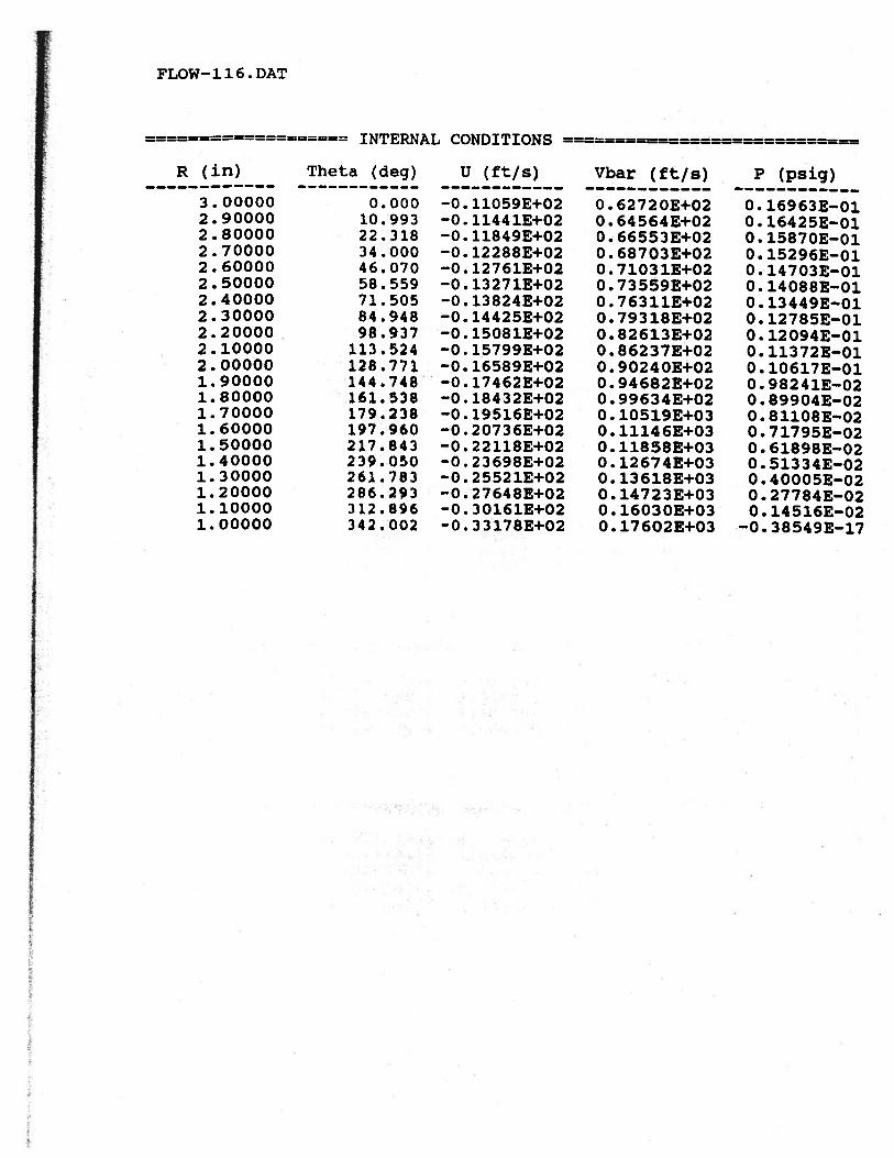
CSUBROUTINE THETA(R1 ,U1 ,V1 ,R2,U2,V2,DTIHE,DTIIETA)CC This subroutine calculates the angular position at each radialC position.CCIMPLICIT DOUBLE PRECISION (A-H, O-Z)

DOUBLE PRECISION RI. ,R2,U1 ,U2,Vi ,V2DTIME,DTHETAC

DTIME = 2.*(R1 - R2)I(U1 + U2)

DTHETA = C (Ri - R2)/(Ri*R2) ).( (R2*Vi + Ri*V2)/(Ui + U2) )

RETtWJIENDCC EOP

Appendix G

Data Files

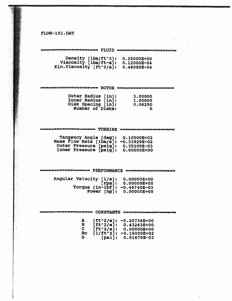
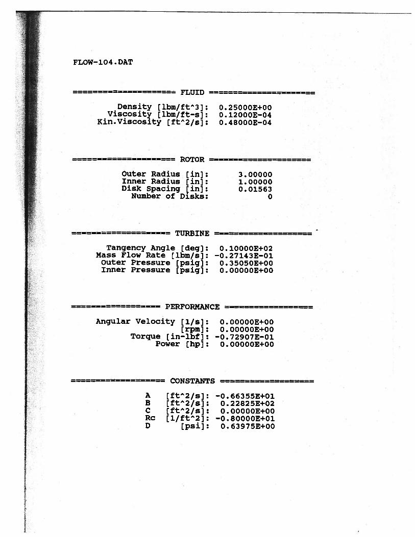
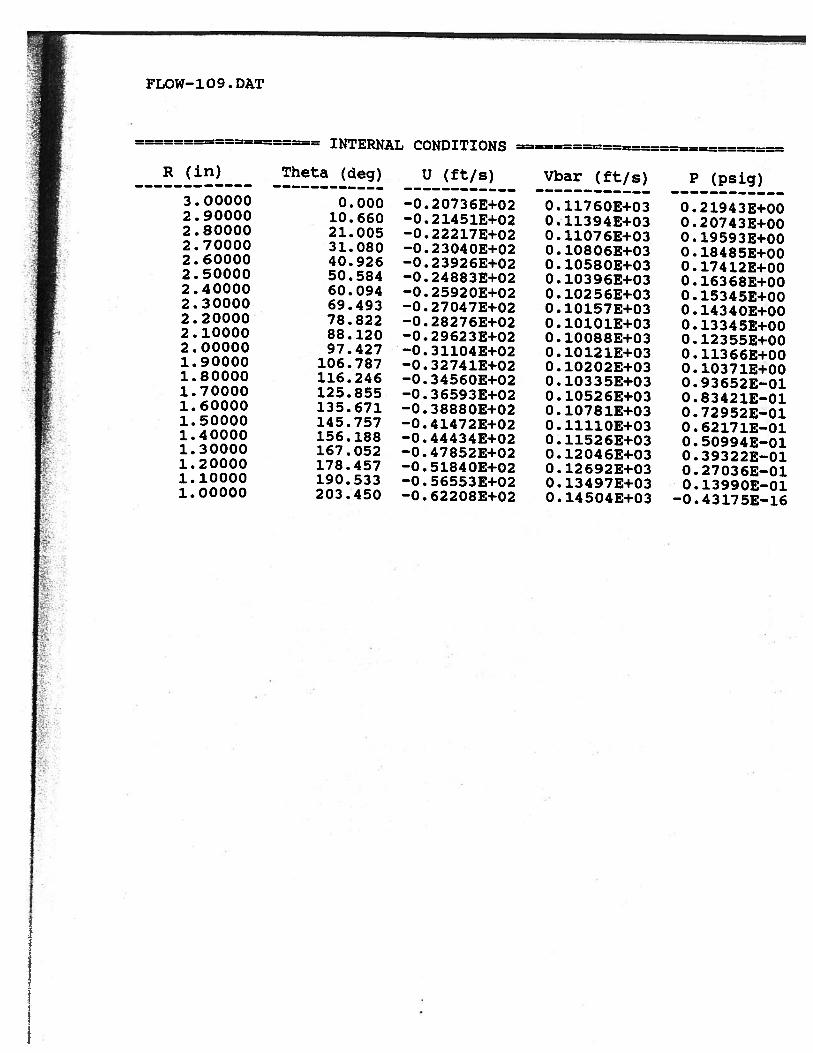
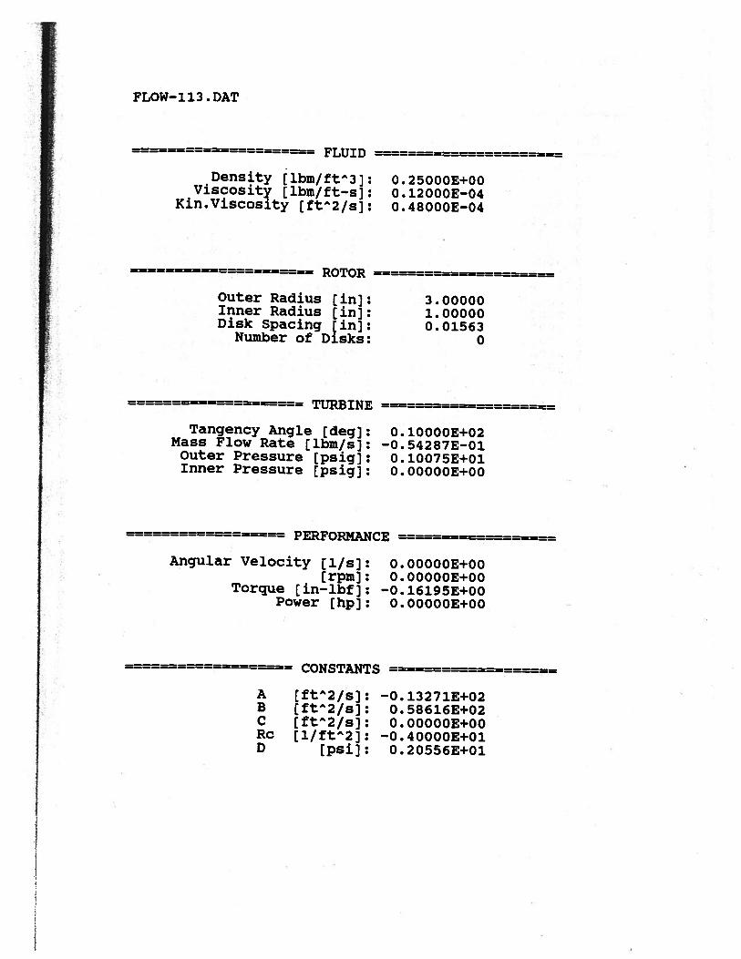
The following pages contain data ifies that were produced by the program listed inAppendix F. What is contained in this appendix is a small sampling of the data filesthat were produced, but this appendix does contain the majority of the data used inthe analysis presented in Chapter 7.

129

FLOW- 100. DAT

:======= FLUID

Density [lbm/ft’3):ViscositV [lbm/ft-s]:

Kin.Viscosity [ft’2/s]:

0.25000E+0O0. 12000E—040. 48000E—04

ROTOR

Outer Radius [in]:Inner Radius [in]:Disk Spacing cm]:

Number of Disks:

:==== TURBINE

Tangency Angle [deg]:Mass Flow Rate [lbm/s]:Outer Pressure [psig]:Inner Pressure [psig]:

3.000001.000000. 06250

0

0.10000E+02—0. 67858E—02

0. 13691E—020.00000E+0O

PERFORMANCE

Angular Velocity [us]:[rpm]:

Torque [in—lbf]:Power [lip]:

0.00000E+00O • 00000E+00

—0.113 92E—02O.00000E+00

CONSTANTS

ABCRcD

[ftA2/s]:[ft’2/s]:

[ft2/s):[1/ft’2]:

[psi]:

—0. 41472E+000. 14265E+010. 00000E+00

—0. 80000E+010. 24990E—02

FLOW- 100. DAT

INTERNAL CONDITIONS

II

I

R (in)

3. 000002.900002.800002.700002. 600002.500002. 400002.300002. 200002. 100002.000001. 900001. 800001. 700001. 600001. 500001. 400001. 300001. 200001. 100001. 00000

Theta (deg)

0.00010. 83821. 70032.61343. 60354.70065. 93477. 33988. 951

100. 810112.963125. 459138. 357151. 725165. 641180. 196195. 503211.695228. 941247. 448267.486

U (ft/s)

—0. 16589E4-01—0. 17161E+01—0. 17774E+01—0. 18432E+01—0. 19141E+01—0. 19906E+01—0.20736E+01—0. 21637E+01—0 • 22621E+01—0. 23698E+01—0.24883E+01—0. 26193E+01—0. 27648E+01—0. 29274E+01—0. 31104E+01—0. 33177E+01—0. 35547E+01—0.38282E+01—0. 41472E+01—0. 45242E+01—0. 49766E+01

Vbar (ft/s)

0. 94079E+010. 94185E+Olf0. 94508E+010. 95059E+01.0 .95851E+02.0. 96900E+010. 98227E+010 .99856E+010. 10182E+020. 10415E+02ô;10689E+020. 11011E+o20.. 11386E+020.1182 4E+020. 12334E+020. 12932E+020.13634E+020.144 64E+02.0.15454E+020.16644E+02

P (psig)

• 0.13691E—020.13 L3OE—020.12570E—020.12008E—ö2

• 0.11443E—02.0. 10874E—O20.10299E—020.97161E—030.91228E—03

• 0.85171E—030. 78967E—030.72588E—030.66004E—03•0.59179E—030.52073E—03

• 0.44637E-030.368 15E—O30.28537E—030 .19718E—030. 10251E—03

0. 18096E+02 —0. 24093E—18

FLOW-lOl .DAT

FLUID

Density [lbm/ftA3]:Viscosity [lbm/ft—s]:

Kin.Viscosity [ftA2/s]:

ROTOR

0. 25000E+000. L2000E—040.48000E—04

Outer Radius [in):Inner Radius [in):Disk Spacing cm):

Number of Disks:

3.000001.000000.06250

0

Tangency Angle [deg):Mass Flow Rate [lbm/s]:Outer Pressure [psig]:Inner Pressure [psig):

0. 10000E+02—0. 33929E—02

0. 35109E—030.00000E+00

PERFORMANCE

Angular Velocity [1/si:[rpm]:

Torque [in-lbf):Power [lip]:

0. 00000E+0O0. 00000E+00

—0.46740E—030.00000E+00

CONSTANTS

TURBINE

A [ft’2/s): —0.20736E+00B £ftA2/s): 0.43263E+00C [ftA2/s): 0.00000E+O0Rc [l/ftA2]: —0.16000E+02D [psi): O.51679E—03

I

FLOW-lOl. DAT

INTERNAL CONDITIONS

R (in)

3. 000002.900002.800002. 700002. 600002. 500002.400002. 300002. 200002. 100002. 000001.900001. 800001.700001. 600001.500001. 400001.300001. 200001.100001.00000

Theta (deg)

0.00010. 66021. 00531. 08040. 92650. 58460. 09469.49378. 82288. 12097.427

106. 787116. 246125. 855135. 671145. 757156. 188167.052178. 457190. 533203. 450

U (ft/s)

—0. 82944E+00—0. 85804E+00—0.888 69E+00—0. 92160E+00—0. 95705E+00—0.9953 3E+00—0. 10368E+01—0. 10819E+O1—0. 11311E+01—0. 11849E+01—0.12442E+01—0. 13096E+01—0. 13824E+01—0. 14637E+01—0. 15552E+01—0. 16589E+01—0. 17774E+01—0. 19 14 1E+01—0.207 36E+01.—0. 22621E+01—0. 24883E+01

Vbar (ft/s)

0. 47040E+010. 45574E+010.443 05E+010. 43223E+010. 42318E+010. 41586E+010. 41023E+010. 40629E+010. 40404E+O10.403 54E+010. 40484E+010. 40808E+010. 41340E+010. 42102E+010. 43123E+010.44441E+010. 46105E+010. 48184E+010. 50770E+010. 53987E+010. 58017E+01

P (psig)

0. 35109E—030. 33188E—030. 31348E—030. 29576E—030.27859E—030. 26188E—030. 24553E—030. 22944E—030.213 52E—030. 19769E—030. 18186E—030.16594E—030. 14984E—030. 13347E—030 • 11672E—030. 99474E—040.8159 1E—040.629 15E—04O • 432 57E—040. 22384E—04

—0 • 60233E—19

I

FLOW-102 .DAT

FLUX D ==============

Density [lbm/ft’3]: 0.25000E+00Viscosity [lbm/ft—s): 0.12000E—04

Kin.Viscosity [ft’2/s]: 0.48000E—04

============= ROTOR

Outer Radius [in]: 3.00000Inner Radius [in): 1.00000Disk Spacing in): 0.03125

Number of Disks: 0

TURBINE

Tangency Angle [deg): O.10000E+02Mass Flow Rate [lbm/s): —0.13572E—OiOuter Pressure [psig): 0.21906E—0iInner Pressure [psig): 0.00000E+00

PERFORMANCE ==

Angular Velocity [ifs): 0.00000E+00[rpm]: 0.00000E+00

Torque [in—lbf]: —0.91134E—02Power [lip): 0.00000E+00

CONSTANTS

A [ft’2/s): —0.i6589E+OiB [ft”2/s): 0.57062E+OiC [ft’2/s]: 0.00000E+00Rc [1/ftA2): —0.80000E+OiD [psi]: O.39984E—0i

FLOW-102 .DAT

INTERNAL CONDITIONS

R (in)

3 . 000002.900002.800002 • 700002 • 600002.500002 • 400002 . 300002. 200002.100002.000001. 900001. 800001. 700001. 600001. 500001. 400001. 300001. 200001.100001. 00000

Theta (deg)

0.00010. 83821. 70032. 61343 • 60454.70065. 93477. 33988. 951

100. 810112.963125. 459138. 358151. 725165. 641180. 196195. 503211.696228. 941247.448267.486

U (ft/s)

—0.663 55E+01—0.68643E+01—0. 71095E+01—0. 73728E+01—0. 76564E+01—0.7962 6E+01—0. 82944E+01—0. 86550E+01—0. 90484E+01—0. 94793E+01—0. 99533E+01—0 • 10477E+02—0. 11059E+02—0. 11710E+02—0. 12442E+02—0. 13271E+02—0. 14219E+02—0.153 13E+02—0.16589E+02—O • 18097E+02—0 • 19907E+02

Vbar (ft/c)

0. 37632E+020. 37674E+020.378 03E+020. 38024E+020. 38340E+020. 38760E+020.39291E+020.39943E+020. 40727E+020 • 4 1659E+020. 42757E+020. 44043E+020. 45544E+020. 47294E+020.493 37E+020. 51728E+020. 54537E+020. 57858E+020.618 15E+020. 66578E+020.72387E+02

P (psig)

0 • 21906E—010. 21008E—010. 20112E—010. 19213E—010.183 1OE—O10. 17399E—010.16479E—010. 15546E—010. 14597E—010 • 13628E—010. 12635E—010 • 11614E—010 • 10561E—010. 94688E—020. 83317E—020. 71420E—020. 58904E—020. 45659E—020. 31548E—020. 16402E—02

—0. 46259E—17

FLOW-103 .DAT

FLUID

Density [lbm/ftA3):Viscosity [lbm/ft-s):

Kin.Viscosity [ftA2/s):

ROTOR

0. 25000E+000. 12000E—040. 48000E—04

Outer Radius [in):Inner Radius [in):Disk Spacing tin):

Number of Disks:

3.000001. 000000.02083

0

Tangency Angle [deg):Mass Flow Rate [lbm/s):Outer Pressure [psig):Inner Pressure [psig):

0.10000E+02—0. 20358E—0l

0. 11090E+000 • 00000E+00

PERFORMANCE

Angular Velocity [us):[rpm):

Torque [in-lbf):Power [lip):

0.00000E+000. 00000E+00

—0.30758E—010. 00000E+00

CONSTANTS

ABCRcD

[ft’2/s):[ft’2/s):[ftA2/s):[l/ftA2):

[psi):

—0 • 373 25E+0l0.12839E+020. 00000E+0O

—0. 80000E+010. 20242E+00

TuRBINE

FLOW-103 .DAT

INTERNAL CONDITIONS

R (in)

3. 000002.900002.800002.700002. 600002. 500002.400002.300002.200002.100002. 000001. 900001. 800001. 700001. 600001. 500001. 400001. 3 00001. 2 00001. 100001.00000

Theta (deg)

0.00010. 83821. 70032.61343. 60454.70065. 93477. 33988. 951

100. 810112.963125. 459138. 358151. 725165. 641180. 196195. 503211. 696228. 941247. 448267.486

U (ft/s)

—0.1493 OE+02—0. 15445E+02—0. 15996E+02—0.16589E+02—0. 17227E+02—0. 17916E+02—0. 18662E+02—0. 19474E+02—0. 20359E+02—0. 21328E+02—0. 22395E+02—0. 23574E+02—0. 24883E+02—0. 26347E+02—0. 27994E+02—0.29860E+02—0. 31993E+02—0. 34454E+02—O.37325E+02—0. 40718E+02—0. 44790E+02

Vbar (ft/s)

0. 84672E+020.847 67E+020. 85057E+020. 85553E+020. 86266E+020.872 11E+020.88405E+020.8987 1E+020. 91636E+020.937 34E+020.962 04E+020. 99097E+020. 10247E+030. 10641E+030.111O1E+030. 11639E+030. 12271E+030. 13018E+030. 13908E+030. 14980E+03O • 16287E+03

P (psig)

0. 1109 OE+000.1063 6E+000. 10181E+000.972 65E—010. 92692E—010.88084E—010.83425E—010. 78701E—010 • 73895E—010. 68989E—010. 63964E—010.587 97E—010. 53464E—010. 47936E—010. 42179E—010. 36156E—010. 29820E—010. 23115E—010. 15971E—O10. 83034E—02

—0. 24672E—16

FLOW-104 .DAT

FLUID

Density [lbm/ftA3):Viscosity [lbiu/ft-s):

Kin.Viscosity [ft’2/s]:

ROTOR

0. 25000E+O00. 12000E—040.48000E—04

Outer Radius [in):Inner Radius tin):Disk Spacing in):

Number of Disks:

3. 000001.000000. 01563

0

Tangency Angle [deg):Mass Flow Rate [lbm/s):

Outer Pressure [psig):Inner Pressure [psig]:

0.10000E+02—0. 27143E—01

0 • 35050E+000.00000E+00

PERFORMANCE


Torque [in—lbf]:Power [hp]:

0. 00000E+00O.00000E+00

—0.72907E—010. 00000E+00

CONSTANTS

{

I

ABCRcD

[ft’2/s):[ftA2/s):[ftA2/s):[1/ftA2]:

[psi):

—0. 66355E+010. 22825E+020. 00000E+00

—0. 80000E+010. 63975E+00

TURBINE

FLOW-104 .DAT

INTERNAL CONDITIONS

R (in)

3 . 000002 . 900002 . 800002 . 700002. 600002 . 500002 . 400002 . 300002.200002. 100002 • 000001. 900001. 800001. 700001. 600001. 500001. 400001.300001. 200001.100001. 00000

Theta (deg)

0.00010. 83821. 70032.61343. 60454. 70065. 93477. 33988. 951

100. 811112.963125. 459138. 358151. 725165.641180. 196195. 503211. 696228.941247. 448267.487

U (ft/s)

—0. 26542E+02—0. 27457E+02—0.284 38E+02—0.2949 1E+02—0. 30626E+02—0. 31851E+02—0. 33178E+02—0. 34620E+02—0. 36194E+02—0. 37917E+02—0. 39813E+02—0. 41909E+02—0.442 37E+02—0. 46839E+02—0.49766E+02—0. 53084E+02—0. 56876E+02—0. 61251E+02—0. 66355E+02—0. 72388E+02—0.79626E+02

Vbar (ft/s)

O.15053E+030.1507 OE+030.1512 1E+030. 15209E+030. 15336E+030.15504E+030.157 16E+030.15977E+030. 16291E+030. 16664E+030. 17103E+030. 17617E+030. 18218E+030. 18918E+030. 19735E+030. 20691E+030. 21815E+030. 23143E+030.2472 6E+030.2663 1E+030. 28955E+03

P (psig)

0. 35050E+O00. 33614E+000. 32178E+O00. 30740E+0O0. 29295E+O00. 27839E+OO0. 26367E+0O0. 24874E+0O0. 23355E+000. 21804E+0O0. 20216E+000. 18583E+000. 16897E+000. 15150E+OO0.1333 1E+0O0.11427E+000.94247 E— 010.73055E—O10. 50478E—010.26243E—O1

—0. 74015E—16

FLOW-105 .DAT

FLUID

Density [lbm/ftA3]:Viscosit( [lbm/ft-s]:


ROTOR

0. 25000E+000. 12000E—040. 48000E—04

Outer Radius (in]:Inner Radius (in]:Disk Spacing cm]:

Number of Disks:

TURBINE

3 • 000001. 000000. 01250

0

Tangency Angle [deg):Mass Flow Rate [lbm/s]:Outer Pressure (psig):Inner Pressure (psig):

0.10000E+02—0.33929E—010.8557 1E+000. 00000E+00

PERFORMANCE

Angular Velocity [ifs]:[rpm):

Torque [in-lbf]:Power [hp):

0.00000E+000.00000E+0O

—0. 14240E+000.00000E+00

CONSTANTS

I

ABCRaD

[ftA2/s):[ft’2/s]:[ft’2/s):[1/ft”2):

[psi):

—0. 10368E+02O • 35664E+020.00000E+00

—O . B0000E+0i0. 15619E+01

FLOw-105. DAT

INTERNAL CONDITIONS

R (in)

3. 000002. 900002.800002.700002. 600002. 500002. 400002.300002. 200002. 100002 . 000001. 900001. 800001. 700001.600001.500001. 400001. 3 00001. 200001.100001. 00000

Theta (deg)

0.00010. 83821. 70032. 61343. 60454.70065. 93477. 33988. 951

100. 810112.963125. 459138. 358151. 725165. 641180. 196195. 503211. 696228. 941247.448267. 486

U (ft/s)

—0. 41472E+02—0. 42902E+02—0. 44434E+02—0. 46080E+02—0. 47852E+02—0. 49766E+02—0. 51840E+02—0. 54094E+02—0. 56553E+02—0.5924 6E+02—0. 62208E+02—0. 65482E+02—0. 69120E+02—0.73 186E+02—0. 77760E+02—0. 82944E+02—0. 88869E+02—0.95705E+02—0. 10368E+03—0. 11311E+03—0. 12442E+03

Vbar (ft/s)

0. 23520E+030. 23546E+030. 23627E+030.23765E+030.23963E+030. 24225E+030. 24557E+030. 24964E+030. 25455E+030. 26037E+030. 26723E+030. 27527E+030 • 28465E+030. 29559E+030. 30836E+030.32330E+030. 34086E+030. 36161E+030. 38634E+030.41611E+030. 45242E+03

P (psig)

0.8557 1E+OO0. 82064E+Ô00. 78561E+000. 75050E+O00. 71522E+000. 67966E+000. 64371E+000. 60726E+000. 57018E-I-O00. 53232E+000.49355E+000.453 68E+O00. 41253E+000. 36987E+000. 32546E+00O • 27898E+000. 23009E+0O0. 1783 6E+000. 12324E+000. 64069E—01

—0. 22204E—15

FLOW-106 .DAT

:========= FLUID

Density [lbm/ftA3):Viscosity [ibm/ft—s]:


ROTOR

0. 25000E+OO0. 12000E—04o . 48000E—04

Outer Radius [in]:Inner Radius [in):Disk Spacing tin]:

Number of Disks:

TURBINE

3. 000001. 000000. 03125

0

Tangency Angle [deg]:Mass Flow Rate [ibm/si:Outer Pressure [psig]:Inner Pressure (psig):

0. 10000E+02—0 • 678 58E-020.5617 5E—020.00000E+00

PERFORMANCE

Angular Velocity [1/s):[rpm]:

Torque [in-ibf]:Power [hp):

0.00000E+000. 00000E+00

—0. 37392E—O20.00000E+00

CONSTANTS

I

I

ABCRcD

[ftA2/s]:

[ft’2/s]:[ft’2/s):[l/ft’2):

[psi]:

—0.82944E+000.173 05E+O10. 00000E+OO

—0. 16000E+020. 82687E—02

FLOW—106 .DAT

INTERNAL CONDITIONS

R (in)

3 . 000002 . 900002 . 800002.700002 . 600002 . 500002 .400002 .300002 . 200002. 100002 . 000001. 900001. 800001. 700001. 600001. 500001.400001. 300001. 200001. 100001. 00000

Theta (deg)

0.00010. 66021. 00531. 08040. 92650. 58460. 09469.49378. 82288.12097. 427

106. 787116.246125. 855135. 671145. 757156. 188167.052178. 457190. 533203.450

U (ft/s)

—0. 33178E+01—0.3432 2E+0I.—0. 35547E+01—0. 36864E+01—0. 38282E+01—0. 39813E+01—0. 41472E+01—0. 43275E+0I.—0. 45242E+01—0. 47397E+01—0. 49766E+01—0. 52386E+01—0. 55296E+01—0. 58549E+01—0.622 08E+01—0.663 55E+01—0. 71095E+01—0. 76564E+01—0. 82944E+01—0. 90484E+01—0.9953 3E+01

Vbar (ft/s)

0.188 16E+020. 18230E+020. 17722E+020. 17289E+020. 16927E+020. 16634E+020. 16409E+020. 16252E+020. 16162E+020.1614 1E+020. 16194E+020.163 23E+020. 1653 6E+020. 16841E+020.17249E+020. 17776E+020. 18442E+020. 19274E+020. 20308E+020. 21595E+020. 23207E+02

P (psig)

0.56175E—020. 53102E—020. 50157E—020. 47321E—020 • 44575E—020. 41901E—020. 39284E—020.367 1OE—020. 34163E—020. 31630E—020. 29097E—020. 26550E—020. 23975E—020. 21356E—020. 18676E—020.159 16E—020. 13055E—020 • 10066E—020 • 692 12E—030. 35814E—03

—0. 96374E—18

FLOW-107 .DAT

FLUID

Density [lbm/ftA3]:Viscosity [lbm/ft-s]:


ROTOR

0. 25000E+00o . 12000E—04o . 48000E—04

Outer Radius [in]:Inner Radius [in):Disk Spacing tin]:

Number of Disks:

3. 000001. 000000.02083

0

Tangency Angle [deg):Mass Flow Rate [lbin/s):Outer Pressure [psig):Inner Pressure [psig]:

0.10000E+02—0.10179E—010. 28439E—010. 00000E+00

PERFORMANCE

Angular Velocity [1/8]:[rpm):

Torque [in-lbf]:Power [hp]:

0. 00000E+000. 00000E+00

—0. 12620E—010. 00000E+00

CONSTANTS

ABCRcD

[ft*2/s):[ftA2/s):[ftA2/s):[l/ftA2):

[psi):

—0.18662E+0l0. 38937E+0l0.00000E+00

—0. 16000E+020. 41860E—0l

TURBINE

FLOW-107 .DAT

INTERNAL CONDITIONS

R (in)

3 . 000002 . 900002.800002.700002 . 600002.500002. 400002. 300002.200002 . 100002. 000001.900001. 800001. 700001. 600001. 500001.400001. 300001. 200001. 100001. 00000

Theta (deg)

0.00010. 66021. 00531. 08040. 92650. 58460. 09469.49378.82288. 12097. 427

106. 787116. 246125. 855135. 671145. 757156. 188167.052178. 457190. 533203.450

U (ft/s)

—0. 74650E+01—0. 77224E+01—0.79982E+01—0.82944E+01—0. 86134E+01—0. 89580E+01—0. 93312E+01—0. 97369E+01—0. 10180E+02—0. 10664E+02—0. 11197E+02—0. 11787E+02—0. 12442E+02—0. 13173E+02—0. 13997E+02—0. 14930E+02—0. 15996E+02—0.172 27E+02—0. 18662E+02—0. 20359E+02—0. 22395E+02

Vbar (ft/s)

0.423 36E+020. 41017E+020. 39875E+020.389 OOE+020.38086E+020.374 27E+020. 36921E+020. 36566E+020.363 64E+020.363 18E+020. 36436E+020. 36727E+020. 37206E+020. 37892E+020.388 11E+020. 39997E+020. 41495E+020.43366E+020.45693E+020 • 48589E+020.522 15E+02

P (psig)

0. 28439E—010. 26883E—010. 25392E—010. 23956E—010. 22566E—010. 21213E—010. 19888E—010.18584E—010. 17295E—010. 16013E—010. 14730E—010.1344 1E—Ol0. 12137E—010.108 11E—Ol0. 94546E—020 • 80574E—020. 66089E—020. 50962E—020. 35039E—020. 18131E—02

—0 • 53969E—17

FLOW-108 .DAT

FLtJID

Density [lbm/ftA3]:Viscosity [lbzn/ft—s):


ROTOR

0. 25000E+000. 12000E—040. 48000E—04

Outer Radius [in):Inner Radius [in]:Disk Spacing tin]:

Number of Disks:

TURBINE

3.000001. 000000. 01563

0


0. 10000E+02—0. 13572E—01

0. 89880E—O10.00000E+00

PERFORMANCE


Torque [in-lbf):Power [hp):

O.00000E+000. 00000E+00

—O • 29913E—010.00000E+00

CONSTANTS

A [ft’2/s]: —0.33178E+01B [ft2/s): 0.69221E+01C [ft”2/s): O.00000E+00Rc [1/ft2): —O.16000E+02D [psi): 0.13230E+00

I

FLOW—108 .DAT

INTERNAL CONDITIONS

R (in)

3 . 000002.900002.800002 . 700002 . 600002 . 500002.400002.300002 . 200002 . 100002 • 000001. 900001. 800001. 700001. 600001. 500001. 400001. 300001. 200001. 10000

Theta (deg)

0.00010. 66021. 00531. 08040. 92650. 58460. 09469. 49378. 82288. 12097. 427

106. 787116. 246125. 855135. 671145. 757156. 188167.052178. 457190. 533

U (ft/s)

—0.1327 1E+02—0. 13729E+02—0.142 19E+02—0. 14746E+02—0.153 13E+02—0. 15925E+02—0.16589E+02—0. 17310E+02—0. 18097E+02—0. 18959E+02—0.19907E+02—0. 20954E+02—0. 22118E+02—0.2342 OE+02—0. 24883E+02—0. 26542E+02—0. 28438E+02—0.3062 6E+02—0. 33178E+02—0. 36194E+02

Vbar (ft/s)

0. 75264E+020.729 19E+02O . 70889E+020. 69156E+020.677 09E+020.6653 8E+020.6563 8E+020.65007E+020. 64647E+020. 64566E+020.64775E+020. 65293E+020. 66144E+020. 67364E+020. 68997E+020. 71105E+020. 73768E+02O . 77095E+020.8123 1E+020. 86380E+02

P (psig)

0.89880E—O10.84963E—010.802 52E—O2.0.757 14E—010. 71320E—O10 • 67042E—010. 62855E—010. 58736E—010. 54660E—010.50608E—010. 46555E—O10. 42480E—010.383 60E—010. 34169E—O10. 29881E—O10. 25465E—010. 20887E—O10. 16106E—010. 11074E—O10 • 573 03E—02

1. 00000 203.450 —0.39813E+02 0.92827E+02 —0.12336E—16

FLOW-109 .DAT

FLUID

Density [lbm/ftA3]:Viscosit’ [ibm/ft-B]:


ROTOR

0. 25000E+000. 12000E—040. 48000E—04

Outer Radius [in]:Inner Radius [in]:Disk Spacing tin):

Number of Disks:

3. 000001.000000. 01250

0

Tangency Angle [deg]:Mass Flow Rate [lbin/s):Outer Pressure [psig):Inner Pressure [psig]:

0. 10000E+02—0. 16965E—01

0. 21943E+000.00000E+00

PERFORMANCE

Angular Velocity [us):[rpm]:

Torque [in-lbf]:Power [lip):

O.00000E+000. 00000E+00

—0. 58424E—010. 00000E+00

CONSTANTS

TURBINE

A [ft’2/s]: —0.51840E+01B [ftA2/s): 0.10816E+02C [ft”2/s): 0.00000E+0ORc [1/ftA2]: —0.16000E+02D [psi): 0.32299E+00

I

FLOW-109 .DAT

INTERNAL CONDITIONS

R (in)

3. 000002. 900002. 800002. 700002.600002. 500002.400002. 300002. 200002. 100002. 000001. 900001. 800001. 700001. 600001. 500001. 400001.300001. 200001. 100001.00000

Theta (deg)

0.00010. 66021. 00531.08040. 92650. 58460. 09469. 49378. 82288. 12097. 427

106. 787116.246125. 855135. 671145. 757156. 188167. 052178. 457190. 533203.450

U (ft/s)

—0.20736E+02—0. 21451E+02—0. 22217E+02—0. 23040E+02—0.2392 6E+02—O.24883E+02—0. 25920E+02—0. 27047E+02—0. 28276E+02—0. 29623E+02—0. 31104E+02—0. 32741E+02—0. 34560E+02—0. 36593E+02—0. 38880E+02—0. 41472E+02—0.44434E+02—0. 47852E+02—0.5184 OE+02—O.56553E+02—0 • 62208E+02

Vbar (ft/s)

0. 11760E+030. 11394E+030.1107 6E+030. 10806E+030. 10580E+030. 10396E+030. 10256E+030. 10157E+030. 1O1O1E+03O.10088E+030.1012 1E+030.102 02E+030. 10335E+030.1052 6E+030. 10781E+030. 1111OE+030.1152 6E+030. 12046E+030. 12692E+030. 13497E+030. 14504E+03

P (psig)

0. 21943E+000. 20743E+000. 19593E+000. 18485E+000.174 12E+000.163 68E+000.153 45E+000.14340E+000. 13345E+000. 12355E+000. 11366E+000.1037 1E+000. 93652E—010.8342 1E—Ol0. 72952E—010. 62171E—010. 50994E—010. 39322E—010. 27036E—010. 13990E—01

—0 • 43175E—16

FLOW-hO .DAT

FLUID

Density [lbm/ftA3):Viscosity [lbm/ft-s):


ROTOR

0. 25000E+000. 12000E—040.48000E—04

Outer Radius [in):Inner Radius (in):Disk Spacing tin):

Number of Disks:

3.000001.000000.06250

0

Tangency Angle (deg]:Mass Flow Rate tlbm/s):Outer Pressure (psig]:Inner Pressure [psig):

0.10000E+02—0. 13572E—010. 39354E—020. 00000E+00

PERFORMANCE

Angular Velocity [ifs):(rpm):


0.00000E+000. 00000E+O0

—0. 25305E—020.00000E+00

CONSTANTS

ABCRcD

[ft’2/s]:[ft’2/s):[ft’2fs):[lfftA2]:

[psi):

—0. 82944E+000. 36635E+010. 00000E+00

—0. 40000E+010.80298E—02

TURBINE

FLOW—lb .DAT

INTERNAL CONDITIONS

R (in)

3 . 000002.900002.800002.700002 . 600002 . 500002.400002.300002.200002. 100002.000001. 900001. 800001.700001. 600001. 500001. 400001. 300001. 200001. 100001. 00000

Theta (deg)

0.00010. 92922. 06033.41945. 03256. 92869.13981. 70294. 658

108. 053121. 940136. 379151. 442167.209183. 778201. 265219.807239. 577260. 783283. 694308. 653

U (ft/s)

—0. 33178E+01—O • 34322E+01—0. 35547E+01—0 • 36864E+01—0. 38282E+01—0.398 13E+01—0. 41472E+01—0.43275E+01—0.45242E+01—0. 47397E+01—0. 49766E+01—0.52386E+01—0. 55296E+01—0. 58549E+01—0. 62208E+01—0. 66355E+01—0. 71095E+01—0.76564E+01—0.82944E+01—0.90484E+01—0.9953 3E+01

Vbar (ft/s)

0.188 16E+020. 19148E+020. 19521E+020. 19937E+020. 20401E+020.209 19E+020. 21496E+020. 22139E+020.22858E+020. 23662E+020. 24564E+020. 25578E+020. 26723E+020. 28021E+020. 29501E+020. 31198E+020. 33158E+020. 35442E+020. 38130E+020.41331E+020.452 OOE+02

P (psig)

0. 39354E—02O.37961E—020. 36543E—020. 35097E—020. 33618E—020. 32104E—020. 30549E—020. 28949E—020.27299E—020. 25592E—020.23823E—020. 21982E—020. 20062E—020. 18051E—020. 15937E—020. 13706E—020.1134 OE—02o • 88163E—030 • 61093E—030. 31850E—03

—0. 77099E—18

FLOW-ill .DAT

FI.1UID

Density [lbni/ft’3):Viscosity [lbm/ft-s):


ROTOR

0. 25000E+000. 12000E—040. 48000E—04


Number of Disks:

3. 000001.000000. 03125

0

Tangency Angle [deg):Mass Flow Rate [lbrn/s):Outer Pressure [psig):Inner Pressure (psig):

0.10000E+02—0. 27143E—010. 62966E—010. 00000E+00

PERFORMANCE

Angular Velocity [us]:(rpm):


O.00000E+000 • 00000E+00

—0. 20244E—010.00000E+00

CONSTANTS

ABCRcD

[ftA2/s]:tftA2/s]:[ft’2/s]:f1/ftA2):

[psi]:

—0.33178E+0l0 • 14654E+020. 00000E+00

—0. 40000E+Ol0. 12848E+00

TURBINE

FLOW-ill .DAT

INTERNAL CONDITIONS

R (in)

3. 000002 . 900002 . 800002.700002. 600002.500002.400002.300002.200002 . 100002. 000001.900001.800001. 700001.600001. 500001.400001.300001. 200001.100001.00000

Theta (deg)

0.00010. 92922. 06033. 41945. 03256. 92869.13981. 70294. 658

108.053121.940136. 379151.442167. 209183.778201. 265219.807239. 577260. 783283. 694308.653

U (ft/s)

—0. 13271E+02—0. 13729E+02—0. 142 19E+02—0.1474 6E+02—0.153 13E+02—0. 15925E+02—0.16589E+02—0.173 1OE+02—0. 18097E+02—0. 18959E+02—0.199 07E+02—0. 20954E+02—0. 22118E+02—0.234 19E+02—0.24883E+02—0. 26542E+02—0. 28438E+02—0. 30625E+02—0. 33178E+02—0. 36194E+02—0. 39813E+02

Vbar (ft/s)

0.752 64E+020. 76593E+020. 78083E+020.797 47E+020. 81604E+020. 83674E+020. 85982E+020.88557E+020.914 32E+020. 94649E+020.982 56E+020.102 31E+030.10689E+030. 11209E+030.118 OOE+030. 12479E+030.132 63E+030. 14177E+030.152 52E+030. 16532E+030. 18080E+03

P (psig)

0.62966E—010.60738E—010. 58469E—010. 56155—010. 53789E—010. 51366E—010.4887 8Er,010.463 18E—010. 43678E—O10. 40948E—010. 38116E-010. 35172E—010. 32099E—010. 28882E—10. 25500E.b10 • 21930E—010. 18143E—010. 14106E—010. 97749E—020. 50960E—02

—0 • 12336E—16

FLOW-112 .DAT

FLUID

Density [lbm/ftA3]: 0.25000E+00Viscosity [lbm/ft—s): 0.12000E—04

Kin.Viscosity [ft’2/s): 0.48000E—04

ROTOR

Outer Radius [in]: 3.00000Inner Radius [in]: 1.00000Disk Spacing cm]: 0.02083

Number of Disks: 0

TURBINE

Tangency Angle [deg): 0.10000E+02Mass Flow Rate [lbm/s): —0.40715E—01Outer Pressure [psig]: 0.31876E+00Inner Pressure [psig): 0.00000E+00

PERFORMANCE

Angular Velocity [us]: 0.00000E+00[rpm]: 0.00000E+00

Torque [in—lbf): —0.68323E—01Power [hp): 0.00000E+00

CONSTANTS ==========

A [ft’2/s): —0.74650E+01B fft2/s]: 0.32971E+02C [ft’2/s): 0.00000E+00Rc [1/ft2): —0.40000E+01D [psi]: O.65042E+00

FLOW-112 .DAT

INTERNAL CONDITIONS

R (in)

3 • 000002. 900002. 800002. 700002. 600002.500002. 400002. 300002. 200002. 100002. 000001.900001.800001. 700001.600001.500001.400001.300001. 200001. 100001. 00000

Theta (deg)

0.00010. 92922.06033.41945. 03256. 92869.13981. 70294.658

108.053121.940136. 379151. 442167.209183.778201. 265219.807239.577260. 783283.694308.653

U (ft/s)

—0. 29860E+02—0. 30890E+02—0. 31993E+02—0. 33178E+02—0.34454E+02—0. 35832E+02—0. 37325E+02—0.38948E+02—0.407 18E+02—0. 42657E+02—0.44790E+02—0. 47147E+02—0 • 497 66E+02—0. 52694E+02—0. 55987E+02—0.5972 OE+02—0. 63985E+02—0. 68907E+02—0. 74650E+02—0.81436E+02—0 • 89580E+02

Vbar (ft/s)

0. 16934E+030.1723 3E+030. 17569E+030.1794 3E+030. 18361E+030. 18827E+030. 19346E+030. 19925E+030.2057 2E+030. 21296E+030. 22108E+030. 23020E+030. 24051E+030.252 19E+030. 26551E+030. 28078E+030.29842E+030. 31898E+030.343 17E+030. 37198E+030. 40680E+03

P (psig)

0. 31876E+000. 30749E+000. 29600E+000.28429E+000.2723 1E+000. 26004E+000. 24745E+000. 23449E+000. 22112E+000. 20730E+0O0. 19296E+000. 17806E+O00. 16250E+000. 14621E+000. 12909E+000. 11102E+000. 91851E—O10. 71412E—010.49486E—010. 25799E—01

—0.863 51E—16

FLOW—113 .DAT

FLUID

Density [lbm/ftA3):Viscosity [lbm/ft-s]:

Kin.Viscosity tftA2/s]:

ROTOR

0. 25000E+000. 12000E—040. 48000E—04


Number of Disks:

TURBINE

3.000001. 000000. 01563

0

Tangency Angle [deg]:Mass Flow Rate [lbm/s):Outer Pressure [psig):Inner Pressure [psig):

0.10000E+02—0.54287E—01

O.10075E+010. 00000E+00

PERFORMANCE

Angular Velocity [us]:[rpm):


0. 00000E+000. 00000E+00

—0. 16195E+00o . 00000E+00

CONSTANTS

ABCRcD

[ftA2/s):[ft’2/s]:[ft’2/s):[1/ftA2]:

[psi):

—0.1327 1E+020. 58616E+020. 00000E+00

—0. 40000E+010. 20556E+01

FLOW-113 .DAT

INTERNAL CONDITIONS

R (in)

3. 000002. 900002. 800002 . 700002. 600002. 500002. 400002.300002.200002. 100002. 000001. 900001.800001. 700001. 600001. 500001. 400001. 300001. 200001.100001.00000

Theta (deg)

0.00010. 92922. 06033. 41945. 03256. 92869. 13981. 70294. 658

108. 053121. 940136. 379151.442167.209183.778201.265219.807239. 577260.783283. 694308.653

U (ft/s)

—0. 53084E+02—0.549 15E+02—0. 56876E+02—0.58982E+02—0.612 51E+02—0. 63701E+02—0. 66355E+02—0. 69240E+02—0. 72387E+02—0. 75835E+02—0 • 79626E+02—0. 83817E+02—0.88474E+02—0. 93678E+02—0. 99533E+02—0. 10617E+03—0.113 75E+03—0. 12250E+03—0.1327 1E+03—0.14477E+03—0.1592 5E+03

Vbar (ft/s)

0. 30106E+030. 30637E+030. 31233E+030. 31899E+030. 32642E+030.33470E+030 • 34393E+030. 35423E+030. 36573E+030. 37860E+030. 39302E+030. 40925E+030. 42757E+030.44834E+030.47202E+030.499 17E+030. 53053E+030. 56707E+030. 61008E+030.6613 OE+030. 72320E+03

P (psig)

0. 10075E+O10. 97181E+000. 93551E+000 • 89848E+000. 86063E+000. 82185E+OO0 • 78205E+000. 74109E+0O0. 69885E1-000. 65516E+0O0. 60986E+0O0.56275E+000 • 513 58E+OO0.462 1OE+0O0. 40800E+0OO • 35088E+000.29029E+OO0. 22570E+000. 15640E+000. 81536E—01

—0, 19737E—15

FLOW-114 .DAT

FLUID

Density [lbm/ftA3):Viscosity [lbm/ft-s]:


ROTOR

o . 25000E+000. 12000E—040.48000E—04

Outer Radius [in]:Inner Radius [in):Disk Spacing cm]:

Number of Disks:

TURBINE

3. 000001. 000000. 01250

0


0. 10000E+02—0. 67858E—010. 24596E+010.00000E+0O

PERFORMANCE

Angular Velocity [us):[rpm]:

Torque [in-lbf):Power [hp]:

0 • 00000E+000 • 00000E+00

—0.3163 1E+O00. 00000E+00

CONSTANTS

ABCRcD

tftA2/s]:[ft’2/s]:[ft’2/s):[1/ftA2]:

[psi):

—0. 20736E+020. 91587E+020.00000E+0O

—0.40000E+010.5018 6E+01

FLOW-114 .DAT

INTERNAL CONDITIONS

R (in)

3. 000002. 900002 . 800002 . 700002. 600002 . 500002.400002.300002.200002. 100002. 000001. 900001. 800001. 700001.600001. 500001. 400001.300001. 200001.100001.00000

Theta (deg)

0.00010. 92922.06033.41945. 03256. 92869. 13981. 70294 .658

108.053121. 940136. 379151. 442167. 209183.778201. 2652 19.807239.577260.783283.694308.653

U (ft/s)

—0. 82944E+02—0. 85804E+02—0. 88869E+02—0. 92160E+02—0.957 05E+02—0. 99533E+02—0. 10368E+03—0. 10819E+03—0.113 11E+03—0. 11849E+03—0. 12442E+03—0. 13096E+03—0. 13824E+03—0. 14637E+03—0. 15552E+03—0. 16589E+03—0. 17774E+03—0. 19141E+03—0. 20736E+03—0.22621E+03—0. 24883E+03

Vbar (ft/s)

0.4704 OE+030.4787 1E+030.488 02E+030. 49842E+030. 51002E+030. 52296E+030. 53739E+030.553 48E4-030. 57145E+030. 59156E+030.614 1OE+030. 63946E+030.668 08E+030. 70053E+030.737 52E+030.77995E+030.8289 5E+030. 88605E+030.953 24E+030.103 33E+040.113 OOE+04

P (psig)

0. 24596E+010. 23726E+010.2284 OE+010. 21936E+O10. 21011E+010. 20065E+010.19093E+O10. 18093E+O10. 17062E+010. 15995E+O10. 14889E+010. L3739E+O10. 12539E+010.112 82E+010.99608E+000. 85663E+000. 70873E+000. 55102E+000. 38183E+000. 19906E+00

—0.49343E—15

FLOW-015 .DAT

======—====——========= FLUID

Density [lbm/ftA3): 0.25000E+00Viscosity [lbm/ft—s): O.12000E—04

Kin.Viscosity (ft’2/s): 0.48000E—04

ROTOR

Outer Radius [in): 3.00000Inner Radius [in]: 1.00000Disk Spacing tin]: 0.01042

Number of Disks: 0

TURBINE

Tangency Angle [deg]: O.10000E+02Mass Flow Rate [lbm/s): —0.81430E—01Outer Pressure [psig): 0.51002E+O1Inner Pressure [psig): O.00000E+00

PERFORMANCE

Angular Velocity [us): O.00000E+00[rpm): 0.00000E+00

Torque [in—lbf): —O.54657E+00Power [hp]: 0.00000E+00

CONSTANTS

A [ft’2/s): —O.29860E+02B [ft’2/s): 0.13188E+03C [ftA2/s): 0.00000E+00Rc [1/ftA2): —0.40000E+01D [psi]: O.10407E+02

FLOW-O 15 .DAT

INTERNAL CONDITIONS

R (in)

3.000002 . 900002 . 800002. 700002. 600002. 500002. 400002. 300002. 200002. 100002. 000001. 900001.800001. 700001.600001. 500001. 400001.300001. 200001.100001.00000

Theta (deg)

0.00010. 92922.06033.41945. 03256. 92869.13981. 70294. 658

108.053121. 940136. 379151.442167. 209183. 778201. 265219. 807239. 577260. 783283.694308. 653

U (ft/s)

—0. 11944E+03—0. 12356E+03—0. 12797E+03—0 • 13271E+03—0. 13781E+03—0. 14333E+03—0. 14930E4-03—0. 15579E+03—0. 16287E+03—0. 17063E+03—0. 17916E+03—0. 18859E+03—0. 19906E+03—0. 21077E+03—0. 22395E+03—0. 23888E+03—0. 25594E+03—0. 27563E+03—0. 29860E+03—0. 32574E+03—0. 35832E+03

Vbar (ft/s)

0.677 37E+030.6893 3E+030. 70274E+030. 71772E+030.73443E+030.753 06E+030.773 84E+030.797 O1E+030. 82289E+030. 85183E+030.884 30E+030 • 92081E+030.962 03E+030. 10088E+040. 10620E+040.112 31E+040.119 37E+040.127 59E+040.13727E+040.14879E+040. 16272E+04

P (psig)

O.51002E+010. 49197E+010.473 60E+010. 45485E+O10. 43569E+010 • 41606E+010. 39591E+010.37517E+010. 35379E+010. 33167E+010. 30874E+O1.0.28489E+010. 26000E+010. 23394E+010. 20654E+O10. 17763E+010. 14696E+010 • 11426E+010 • 79176E+O00 • 41277E+00

—0. 11842E—14

FLOW- 116. DAT

FIt3ID

Density (lbm/ftA3):Viscosity [lbm/ft-s]:


ROTOR

o • 25000E+0O0. 12000E—040. 48000E—04

Outer Radius [in]:Inner Radius [in):Disk Spacing tin):

Number of Disks:

3.000001. 000000. 06250

0

Tangency Angle [deg):Mass Flow Rate [lbm/s):Outer Pressure [psig):Inner Pressure [psig]:

0.100 OOE+02—0. 45239E—01

0. 16963E—010. 00000E+00

PERFORMANCE

Angular Velocity [1/s):[rpm):


0.000OOE+000. 00000E+00

—0. 90999E—020. 00000E+00

CONSTANTS

ABCRcD

[ft’2/s):[ftA2/s):[ftA2/s):[1/ftA2):

[psi):

—0, 27648E+010. 14547E+020. 00000E+00

—0. 12000E+010. 37592E—01

TURBINE

FLOW—116 .DAT

INTERNAL CONDITIONS

R (in)

3. 000002.900002.800002.700002. 600002. 500002.400002.300002.200002. 100002. 000001. 900001. 800001. 700001. 600001.500001. 4 00001. 300001. 200001.100001. 00000

Theta (deg)

10. 99322. 31834.00046. 07058. 55971. 50584.94898.937

113.524128.77].144.748161.538179.238197.960217.843239.050261.763286. 2933 12.896342 • 002

U (ft/s)

—0. 11059E+02—0. 1144 1E+02—0.11849E+02—0. 12288E+02—0. 12761E+02—0.13271E+02—0. 13824E+02—0. 14425E+02—0. 1508 1E+02—0.15799E+02—0.16589E+02—0. 17462E+02—0. 18432E+02—0. 19516E+02—0. 2073 6E+02—0. 22118E+02—0. 23698E+02—0 • 2552 1E+02—0.27648E+02—0. 30161E+02-0. 33178E+02

Vbar (ft/s)

0.6272 OE+020. 64564E+020.66553E+020. 68703E+020.7103 1E+020. 73559E+020 • 763 11E+020.793 18E+020. 82613E+020.862 37E+020. 90240E+020. 94682E+020.9963 4E+020.10519E+030. 11146E+030.118 58E+030. 12674E+030. 13618E+030. 14723E+030. 16030E+030. 17602E+03

P (psig)

0. 16963E—0j.0. 16425E—010. 15870E—010. 15296E—010. 14703E—010. 14088E—010. 13449E—010. 12785E—010. 12094E—010. 11372E—010.10617E—01.0. 98241E—020 • 89904E—020. 81108E—020. 71795E—020. 61898E—020.513 34E—020. 40005E-020.27784E—020. 14516E—02

—0. 38549E—17

FLOW- 117. DAT

FLUID

Density [lbm/ft’3]:Viscosity [lbm/ft-s):


ROTOR

o . 25000E+000. 12000E—040. 48000E—04


Number of Disks:

3. 000001. 000000.03125

0

Tangency Angle [deg]:Mass Flow Rate [lbm/s]:Outer Pressure [psig]:Inner Pressure [psig):

0. 10000E+02—0.90478E—010.2714 1E+000.00000E+00

PERFORMANCE



0.00000E+000. 00000E+00

—0. 72799E—010.00000E+00

CONSTANTS

A [ftA2/s):B [ftA2/s):C [ftA2/s):

Rc [1/ftA2]:D [psi):

—0 • 11059E+020. 58188E+020.00000E+00

—0. L2000E+010. 60148E+00

TURBINE

FLOW— 117. DAT

INTERNAL CONDITIONS

R (in)

3 . 000002 . 900002.800002 . 700002 . 600002.500002 .400002. 300002 .200002 . 100002 . 000001.900001. 800001. 700001. 600001.500001. 400001. 300001. 200001.100001. 00000

Theta (deg)

0.00010.99322.31834 . 00046. 07058. 55971. 50584.94898.937

113.524128.771144.748161. 538179. 238197. 960217.843239.050261. 783286. 293312.896342 • 002

U (ft/s)

—0.44237E+02—0. 45762E+02—O . 47397E+02—0. 49152E+02—0. 51042E+02—0. 53084E+02—0. 55296E+02—0. 57700E+02—0. 60323E+02—0. 63195E+02—0.663 55E+02—0.69848E+02—0.73728E+02—0. 78065E+02—0. 82944E+02—0. 88474E+02—O . 94793E+02—0. 10208E+03—0.11059E+03—0. 12065E+03—0. 13271E+03

Vbar (ft/s)

0. 25088E+030.2582 6E+030. 26621E+030. 27481E+030 • 28412E+030.29423E+030. 30525E+030 • 31727E+030. 33045E+030 • 34495E+030. 36096E+030. 37873E+030. 39854E+030. 42075E+030. 44582E+030. 47431E+03O.50697E+030. 54474E+030. 58890E+030. 64121E+030.704 1OE+03

P (psig)

0. 27141E+O0O • 26280E+000. 25392E+OO0. 24474E+0O0. 23524E+000. 22540E+000. 21519E+000. 20457E+000. 19350E+00O • 18195E+00O • 1698 6E+00O • 157 18E+00O.14385E+00O.12977E+O00. 11487E+00O • 99037E—01O • 8213 5E—010. 64007E—010.444 55E—010. 23226E—01.

—O • 61679E—16

FLOW-118 .DAT

FLUX D

Density [lbm/ftA3): 0.25000E+00Viscosity [lbm/ft—s]: 0.12000E—04

Kin.Viscosity [ft’2/s): 0.48000E—04

ROTOR =============:

Outer Radius [in]: 3.00000Inner Radius [in]: 1.00000Disk Spacing cm): 0.02083

Number of Disks: 0

PtJR.B INE

Tangency Angle [deg): 0.10000E+02Mass Flow Rate [lbm/s]: —0.13572E+00Outer Pressure [psig]: 0.13740E+0lInner Pressure [psig): 0.00000E+00

PERFORMANCE

Angular Velocity [us]: 0.00000E+00[rpm): 0.00000E+O0

Torque [in—lbf): —0.24570E+00Power [tip]: 0.00000E+00

: CONSTAN’tI’S

A [ftA2/s]: —0.24883E+02B [ft’2/s): 0.13092E+03C [ft’2/s): 0.00000E+00Rc [u/ftA2): -0.12000E+0lD [psi): 0.30450E+0l

FLOW—118 .DAT

INTERNAL CONDITIONS

R (in) Theta (deg) U (ft/s) Vbar (ft/s) P (psig)

3.00000 0.000 —0.99533E+02 O.56448E+03 O.13740E+012.90000 10.993 —0.10297E+03 O.58108E+03 O.13304E+012.80000 22.318 —0.10664E+03 O.59898E+03 O.12854E+012.70000 34.000 —0.11059E+03 O.61833E+03 0.12390E+0I.2.60000 46.070 —0.11485E+03 O.63928E+03 O.11909E+012.50000 58.559 —0.11944E+03 O.66203E+03 0.11411E+012.40000 71.505 —O.12442E+03 O.68680E+03 O.10894E+012.30000 84.948 —0.12983E+03 0.71386E+03 0.10356E+012.20000 98.937 —0.13573E+03 0.74352E+03 0.97961E+002.10000 113.524 —O.14219E+03 0.77614E+03 0.92113E+002.00000 128.771 —0.14930E+03 O.81217E+03 0.85994E+001.90000 144.748 —O.15716E+03 0.85214E+03 0.79575E+001.80000 161.538 —0.16589E+03 0.89671E+03 0.72822E+001.70000 179.238 —0.17565E+03 0.94669E+03 0.65697E+O01.60000 197.960 —0.18662E+03 O.10031E+04 0.58154E+001.50000 217.843 —O.19907E+03 0.10672E+04 O.50137E+001.40000 239.050 —0.21328E+03 0.11407E+04 0.41581E+O01.30000 261.783 —0.22969E+03 0.12257E+04 0.32404E+001.20000 286.293 -O.24883E+03 0.13250E+04 0.22505E+001.10000 312.896 —0.27145E+03 O.14427E+04 0.11758E+001.00000 342.002 —0.29860E+03 0.15842E+04 —0.34540E—15

Date post:	31-Dec-2021
Category:	Documents
Upload:	others
View:	2 times
Download:	0 times

A MODEL FOR FLUID FLOW BETWEEN PARALLEL, CO-ROTATING ...

Documents