Federal Reserve Bank of New York Staff Reports A Model of Liquidity Hoarding and Term Premia in Inter-Bank Markets Viral V. Acharya David Skeie Staff Report no. 498 May 2011 This paper presents preliminary findings and is being distributed to economists and other interested readers solely to stimulate discussion and elicit comments. The views expressed in this paper are those of the authors and are not necessarily reflective of views at the Federal Reserve Bank of New York or the Federal Reserve System. Any errors or omissions are the responsibility of the authors.
Transcript
Federal Reserve Bank of New York
Staff Reports
A Model of Liquidity Hoarding and Term Premia
in Inter-Bank Markets
Viral V. Acharya
David Skeie
Staff Report no. 498
May 2011
This paper presents preliminary findings and is being distributed to economists
and other interested readers solely to stimulate discussion and elicit comments.
The views expressed in this paper are those of the authors and are not necessarily
reflective of views at the Federal Reserve Bank of New York or the Federal
Reserve System. Any errors or omissions are the responsibility of the authors.
A Model of Liquidity Hoarding and Term Premia in Inter-Bank Markets
Viral V. Acharya and David Skeie
Federal Reserve Bank of New York Staff Reports, no. 498
May 2011
JEL classification: G21, G01, E43
Abstract
Financial crises are associated with reduced volumes and extreme levels of rates for term
inter-bank loans, reflected in the one-month and three-month Libor. We explain such
stress by modeling leveraged banks’ precautionary demand for liquidity. Asset shocks
impair a bank’s ability to roll over debt because of agency problems associated with high
leverage. In turn, banks hoard liquidity and decrease term lending as their rollover risk
increases over the term of the loan. High levels of short-term leverage and illiquidity of
assets lead to low volumes and high rates for term borrowing. In extremis, inter-bank
Acharya: New York University, CEPR, and NBER (e-mail: [email protected]). Skeie:
Federal Reserve Bank of New York (e-mail: [email protected]). The authors thank Sha Lu for
excellent research assistance, Jamie McAndrews for valuable conversations, Hubero Ennis
(discussant), Marvin Goodfriend (editor), and participants at the Workshop on Money Markets and
Payments organized by the Federal Reserve Bank of New York (October 2010) and Carnegie-
Rochester Conference on Public Policy (November 2010). The views expressed in this paper are
those of the authors and do not necessarily reflect the position of the Federal Reserve Bank of New
York or the Federal Reserve System.
1 Introduction
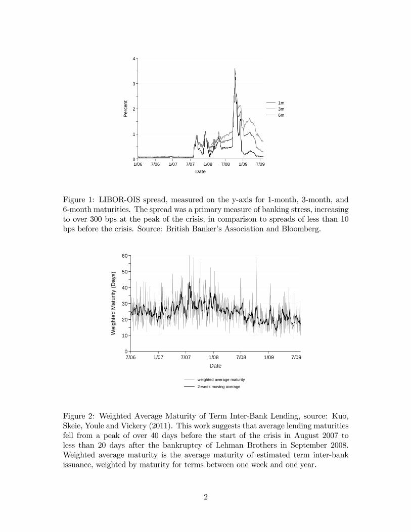
Extreme levels of inter-bank lending rates, particularly at longer maturities, were
seen as a principal market friction of the �nancial crisis of 2007-09. Figure 1 shows
that the spreads between London Interbank O¤er Rate (LIBOR) and Overnight
Indexed Swap (OIS) rate for 1-month, 3-month, and 6-month terms increased to
over 300 bps at the peak of the crisis compared to less than 10 bps before the
crisis.1 Figure 2 shows the weighted-average maturity of inter-bank term lending
estimated by Kuo, Skeie, Youle and Vickery (2011).2 This work suggest that lending
maturities fell from a peak average term of over 40 days before August 2007 to less
than 20 days after the bankruptcy of Lehman Brothers in September 2008.3 Such
rising inter-bank term rates have been widely interpreted as a manifestation of rising
counterparty risk of borrowing banks. However, during the crisis, banks with even
the best credit quality borrowed in term markets at extremely high spreads to the
risk-free rate, suggesting that lenders demanded heightened compensation for term
lending even from relatively safe borrowers.
We provide an explanation of this rise in spreads and a collapse in maturities
in the term inter-bank market by building a model of lending banks�precautionary
demand for liquidity. Our key insight is that each bank�s willingness to provide
term lending (for a given counterparty risk of its borrower) is determined by its
own rollover risk, which is the risk that it will be unable to roll over its debt that
matures before the term of the loan. If adverse asset shocks materialize in the
interim, debt overhang can prevent highly leveraged banks from being able to raise
�nancing required to pay o¤ creditors. Thus, during times of heightened rollover
1The LIBOR-OIS spread is a measure of the credit and liquidity term spread to the risk-freerate for inter-bank loans. LIBOR is a measure of banks� unsecured term wholesale borrowingrates. OIS is a measure of banks�expected unsecured overnight wholesale borrowing rates for theperiod of the �xed-for-�oating interest rate swap settled at maturity, where the �oating rate is thee¤ective (average) fed funds rate for the term of the swap.
2A caveat with estimates of inter-bank activity (both overnight and term) is that their qualityis not currently known.
3Consistent with this, Ashcraft, McAndrews and Skeie (2010) and Afonso, Kovner and Schoar(2010) document that volumes in overnight inter-bank markets did not fall much during the crisisin contrast to the collapse in term lending volumes.
1
0
1
2
3
4
Per
cent
1/06 7/06 1/07 7/07 1/08 7/08 1/09 7/09
Date
1m3m6m
Figure 1: LIBOR-OIS spread, measured on the y-axis for 1-month, 3-month, and6-month maturities. The spread was a primary measure of banking stress, increasingto over 300 bps at the peak of the crisis, in comparison to spreads of less than 10bps before the crisis. Source: British Banker�s Association and Bloomberg.
0
10
20
30
40
50
60
Wei
ghte
d M
atur
ity (D
ays)
7/06 1/07 7/07 1/08 7/08 1/09 7/09
Date
weighted average maturity
2week moving average
Figure 2: Weighted Average Maturity of Term Inter-Bank Lending, source: Kuo,Skeie, Youle and Vickery (2011). This work suggests that average lending maturitiesfell from a peak of over 40 days before the start of the crisis in August 2007 toless than 20 days after the bankruptcy of Lehman Brothers in September 2008.Weighted average maturity is the average maturity of estimated term inter-bankissuance, weighted by maturity for terms between one week and one year.
2
risk, banks �hoard� liquidity by lending less and more expensively at longer term
maturities.4 Elevated rates for term borrowing, in turn, aggravate the debt overhang
and rollover risk problems of borrowing banks. Even strong banks are forced to cut
back on borrowing term and potentially bypass pro�table investments such as real-
sector lending for long-term and illiquid projects.5
In the extremis, there can be a complete freeze in the inter-bank market, in
the sense that there is no interest rate at which inter-bank lending will occur. In
particular, even when banks with pro�table investment opportunities do not have
solvency or liquidity risk, they may be unable to access liquidity on the inter-bank
market if the lending banks have high enough short-term leverage and asset illiquid-
ity. In these cases, paying lending banks their opportunity cost of liquidity renders
borrowers� investments unpro�table. More generally, when the banking sector is
weak (fewer pro�table investments, high uncertainty about asset quality and high
short-term leverage), lenders�precautionary demand for liquidity manifests as low
volumes and high rates in term inter-bank lending.
The key feature of our model �rollover risk of banks central to the inter-bank
markets �was key to the ignition of the �nancial crisis of 2007-09. Acharya, Schnabl
and Suarez (2009) show empirically that the onset of the crisis in August 2007 was
due to commercial bank exposures to o¤-balance sheet vehicles (conduits and SIVs).
These vehicles held securities (primarily, sub-prime mortgage backed) that were
funded with extremely short-dated asset-backed commercial paper (ABCP). Hit by
worsening house prices and the BNP Paribas�public announcement on August 8,
4The Global Head of Loan Syndications & Trading for BNP Paribas explains that �many lendersintermix cost of risk and cost of funding whereas clearly they re�ect two very di¤erent elements.First, their own risk as perceived by their own lenders, and second the risk of the borrower �putanother way, a poor quality borrower and a poor quality lender should result in a very high overallcost to the borrower, conversely the opposite would also apply.�(van Kan, 2010)
5We develop these ideas in a model that builds upon the asset-substitution or risk-shiftingmodel of Jensen and Meckling (1976), Stiglitz and Weiss (1981), Diamond (1989, 1991), and morerecently, Acharya and Viswanathan (2011). In essence, these papers provide a micro-economicfoundation for the funding constraints of a leveraged �nancial �rm: the �rm can switch to a riskier,negative net present value investment (�loan�) after borrowing from �nanciers. In anticipation,the �nanciers are willing to lend to the �rm only up to a threshold level of funding so as to ensurethere is enough equity to keep the �rm�s risk-shifting incentives in check.
3
2007 that sub-prime assets had become practically illiquid, the o¤-balance sheet
vehicles � and, in turn, the commercial banks facing draw downs on credit lines
provided to the vehicles �incurred signi�cant rollover risk.6 Acharya, Schnabl and
Suarez (2009) also document that outstanding short-term ABCP fell by the end of
2008 to half of its level of $1.2 billion in August 2007. Our model suggests that
this rollover risk induced precautionary demand for liquidity in banks, causing term
inter-bank spreads to rise �and volumes to shrink �dramatically.
It is interesting to contrast our analysis to the traditional view of banking panics
and runs. In the canonical model of Diamond and Dybvig (1983), banks fail be-
cause of liquidity demand by retail depositors. These depositors receive exogenous
liquidity shocks and demand immediacy of payments precipitating bank runs. Our
model can be viewed as one in which the liquidity needs of wholesale �nanciers play
a crucial role. These providers, such as banks and money market funds, are funded
with short-term debt themselves and face rollover risk when adverse asset shocks
materialize. In Diamond and Dybvig style runs, there is an ine¢ cient liquidation
of banking assets. In our model, liquidity demand by wholesale �nanciers leads to
bypassing of pro�table investment opportunities, such as lending to the real sector.
It is equally interesting to contrast our analysis with the alternative view that
borrowing rates and volumes in the inter-bank market are determined primarily
by the credit risk of borrowers. Under this view, an increase in the credit risk of
borrowing banks increases lending rates to compensate lenders for the higher risk and
could also lead to reduced volumes. Our analytical framework predicts that spreads
in term inter-bank markets can be larger, and volumes smaller, than ones based
purely on borrower credit risk. At a minimum, this suggests caution in interpreting
the entire rise in term inter-bank rates as being attributable to counterparty risk
concerns.7 Further, our model�s most important and novel implication is that a
6This risk of being unable to acquire short-term funding, in order to honor draw downs oncredit lines backing the illiquid assets funded by ABCP, is equivalent to the more general risk forbanks of being unable to roll over short-term borrowing against illiquid long-term assets.
7Current research appears to have been unable to rationalize the extreme spreads in the inter-bank market as per this borrower-risk channel alone. While Taylor and Williams (2008a, 2008b)
4
bank�s borrowing rate for a particular maturity in the inter-bank market increases
with the credit risk and liquidity risk of its lender, controlling for the borrower�s
own credit risk. In the same vein, bilateral inter-bank markets can freeze even for
some healthy borrowers when most other banks are leveraged, especially at short
maturities, and are holding riskier and more illiquid assets. These implications are
inconsistent with a pure borrower-risk view of inter-bank rates and volumes.
The remainder of the paper is organized as follows. Section 2 sets up our bench-
mark model of inter-bank lending supply and examines how asset illiquidity can
lead to decreases in inter-bank lending. Section 3 extends the model to consider
rollover risk and precautionary behavior on both supply and demand sides of the
inter-bank market. Section 4 relates the results to existing empirical evidence, de-
rives new empirical and policy implications, and discusses the related literature on
liquidity hoarding by banks. Section 5 concludes. Details of proofs and analysis of
the borrowing bank demand are contained in the appendix.
2 Liquidity hoarding
We build a model in which a bank with surplus liquidity either hoards it for its
own future liquidity needs or lends the liquidity in the term inter-bank market to
another bank that has additional capacity for investment in a long-term, illiquid
asset. In Section 2.1, we introduce the benchmark model, in which the lending bank
has existing risky assets and short-term debt in place. We show as a benchmark that
absent any frictions, the lending bank�s own credit risk and leverage do not lead the
bank to hold any liquidity. The bank supplies its full liquidity for term inter-bank
lending. In Section 2.2, we add a moral hazard problem for the lending bank aimed
at capturing opacity and illiquidity of banking assets and activities. The illiquidity
of the lending bank�s assets decreases its ability to roll over its short-term debt.
attribute the large one-month and three-month LIBOR-OIS spreads (as shown in Figure 1) primar-ily to counterparty credit risk, McAndrews, Sarkar and Wang (2008), Michaud and Upper (2008)and Schwarz (2009) attribute most of the spread to liquidity risk, whereas Smith (2010) arguesthat time-varying risk premia explain half of the variation in spreads.
5
Because of this, the lending bank retains liquidity to pay o¤ short-term debt rather
than lend on the term inter-bank market. Term inter-bank lending may thus fall
relative to the benchmark amount even in the absence of credit risk of the borrowing
bank.
2.1 Benchmark model of the term inter-bank market
There are three periods, dates t = 0; 1; 2; and two types of banks i = B;L. At date
0, each bank has in place investment in one unit of a long-term asset that pays at
date 2 y with probability �; corresponding to success of the investment, and zero
otherwise, corresponding to failure of the investment. Thus, the expected return on
the asset is �y � 1. (In Section 3, we will allow � to be a random variable that
is realized at date 1 to allow for the partial revelation of information ex-interim).
Bank i = B is called the �borrowing bank�because it has an opportunity at date
0 for additional investment of up to one unit into the long-term asset but has no
additional liquid goods, which we call �liquidity,�required for the investment. The
bank also does not have any additional borrowing sources from outside depositors
(at least not in the very short term).
To start with, the focus of the model is on bank i = L, called the �lending bank.�
At date 0, this bank has an additional unit of liquidity but has no opportunity for
additional investment in the long-term asset. The bank lends l � 1; which is a
two-period term inter-bank loan, to the borrowing bank at a term interest rate of r
and stores liquidity (1� l) for a rate of return of one for one period. The borrowing
bank invests the two-period term inter-bank loan amount that is borrowed into the
long-term asset and repays the loan at date 2 with probability �.
At date 1, the lending bank has to repay short-term debt �L 2 [1; 2] held by
depositors.8 The bank can repay the debt with liquidity it holds, (1 � l); and by8The amount �L re�ects the lending bank�s e¤ective short-term leverage in place. This leverage
can alternatively be thought of as a broader type of liquidity need, such as the draw-down of thebank�s extended credit lines to corporations or special purpose vehicles. At the minimum value of�L, the bank has su¢ cient liquidity to repay all short-term debt at date 1. At the maximum valueof �L, the bank�s one unit of the long-term asset in place is entirely �nanced by short-term debt.
6
issuing new debt to depositors with a face amount fL due at date 2. The bank
defaults if it cannot repay or roll over its debt, in which case the proceeds of the
bank�s asset-in-place and inter-bank loan have no salvage value to either the bank�s
depositors nor itself.9 Depositors must break even on their expected return �fL to
be willing to roll over debt �L � (1 � l) according to their individual rationality
constraint
�L � (1� l) � �fL: (1)
For a given term inter-bank market rate r; the bank chooses (i) date 0 term lending l
and (ii) date 1 borrowing with face amount fL (due at date 2) in order to maximize
its expected pro�t
�L = �(y + lr � fL); (2)
subject to constraint (1). The optimal values l� and fL� satisfy the �rst order
condition and the depositor rationality constraint, respectively. Substituting from
(1), expected pro�t can be written as �L = �y + l(�r � 1) � �L + 1: The lending
bank�s solution is to lend fully, l� = 1; at any term rate r � 1�: This gives the bank
a risk-adjusted expected rate of return at least that of storage, �r � 1: The bank
lends nothing otherwise, l� = 0 for r < 1�.
Next, we consider a simpli�ed term inter-bank loan demand by a borrowing
bank. The borrowing bank maximizes expected pro�ts by borrowing a full unit at
any term rate below the rate of return on investment, so as to increase investment
in the asset in place. In other words, the borrowing bank has a perfectly elastic
demand to borrow at any term rate that is below the rate of return that investment
pays, b�(r) = 1 for r � y, and does not borrow otherwise, b�(r) = 0 for r > y. To
summarize, with no frictions, the lending bank in equilibrium fully lends its liquidity
at any positive expected rate of return. For � < 1; credit risk of the borrower is
re�ected in the term lending rate in the inter-bank market of r� = 1�> 1 but does
not a¤ect term inter-bank lending volume.
9For instance, these assets are rendered worthless by disintermediation of the bank or illiquidfor a while due to its bankruptcy.
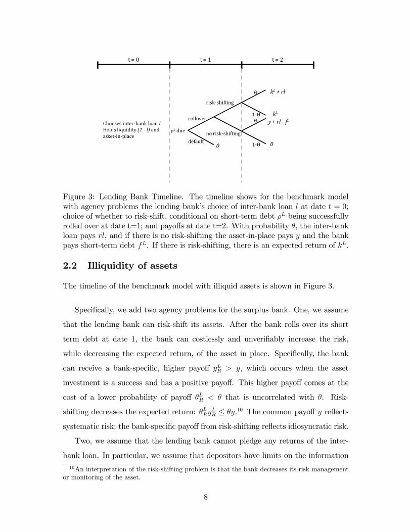
Figure 3: Lending Bank Timeline. The timeline shows for the benchmark modelwith agency problems the lending bank�s choice of inter-bank loan l at date t = 0;choice of whether to risk-shift, conditional on short-term debt �L being successfullyrolled over at date t=1; and payo¤s at date t=2. With probability �, the inter-bankloan pays rl, and if there is no risk-shifting the asset-in-place pays y and the bankpays short-term debt fL. If there is risk-shifting, there is an expected return of kL.
2.2 Illiquidity of assets
The timeline of the benchmark model with illiquid assets is shown in Figure 3.
Speci�cally, we add two agency problems for the surplus bank. One, we assume
that the lending bank can risk-shift its assets. After the bank rolls over its short
term debt at date 1, the bank can costlessly and unveri�ably increase the risk,
while decreasing the expected return, of the asset in place. Speci�cally, the bank
can receive a bank-speci�c, higher payo¤ yLR > y, which occurs when the asset
investment is a success and has a positive payo¤. This higher payo¤ comes at the
cost of a lower probability of payo¤ �LR < � that is uncorrelated with �. Risk-
shifting decreases the expected return: �LRyLR � �y.10 The common payo¤ y re�ects
systematic risk; the bank-speci�c payo¤ from risk-shifting re�ects idiosyncratic risk.
Two, we assume that the lending bank cannot pledge any returns of the inter-
bank loan. In particular, we assume that depositors have limits on the information10An interpretation of the risk-shifting problem is that the bank decreases its risk management
or monitoring of the asset.
8
they can verify about the lending bank�s three types of assets, depending on their
opacity. First, inter-bank loans are the most opaque assets to depositors. The
lending bank itself can verify returns on its inter-bank loan, re�ecting its ability
for peer monitoring. However, the depositors of the lending bank cannot verify any
information about the returns of the inter-bank loan because they are the furthest
removed from the borrowing bank�s assets that ultimately back the inter-bank loan.
Second, the asset in place is held directly by the lending bank and is less opaque
to the bank�s depositors than inter-bank loan is. The depositors can verify whether
the return on the asset in place is positive or zero, but cannot distinguish between
whether a positive return is y or yLR:11 Third, liquidity held by the bank is perfectly
veri�able by depositors, and can be paid out to depositors at date 1.
An increase in term lending by the bank decreases the liquidity (1 � l) that is
available to pay depositors at date 1. However, since returns on inter-bank loans
are fully internalized by the lending bank, it would not attempt to increase the risk
of these returns. This, however, is not the case for the bank�s incentives to increase
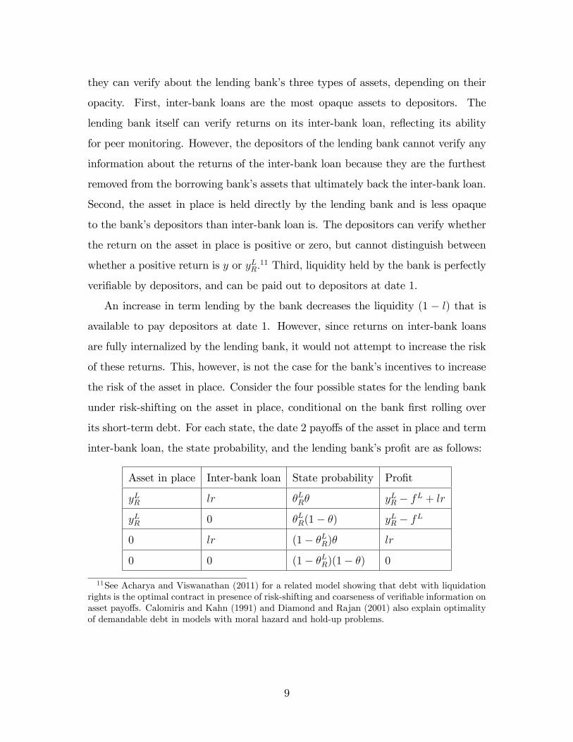
the risk of the asset in place. Consider the four possible states for the lending bank
under risk-shifting on the asset in place, conditional on the bank �rst rolling over
its short-term debt. For each state, the date 2 payo¤s of the asset in place and term
inter-bank loan, the state probability, and the lending bank�s pro�t are as follows:
Asset in place Inter-bank loan State probability Pro�t
yLR lr �LR� yLR � fL + lr
yLR 0 �LR(1� �) yLR � fL
0 lr (1� �LR)� lr
0 0 (1� �LR)(1� �) 0
11See Acharya and Viswanathan (2011) for a related model showing that debt with liquidationrights is the optimal contract in presence of risk-shifting and coarseness of veri�able information onasset payo¤s. Calomiris and Kahn (1991) and Diamond and Rajan (2001) also explain optimalityof demandable debt in models with moral hazard and hold-up problems.
9
The expected pro�t from risk shifting conditional on rolling over debt is thus12
�LR = �LR(y
LR � fL) + �lr: (3)
The lending bank�s incentive compatibility constraint requires that pro�ts with-
out risk-shifting given by equation (2) are greater than pro�ts with risk-shifting
given by equation (3). This incentive constraint can be written as
�(y � fL) � �LR(yLR � fL); (4)
and it holds if and only if the probability of asset payo¤ � is large enough that new
debt is fL � �y��LRyLR���LR
: For tractability, we assume the risk-shifting payout yLR to the
lending bank increases as the probability of success �LR decreases. In the limit, as
�LR ! 0; we assume that yLR ! 1 and �LRyLR ! kL; where kL equals the expected
return of the risk-shifting assets. The value kL is our measure of the illiquidity of
the asset in place. We also refer to kL as the severity of the moral hazard problem.
It is equivalent to an amount of expected pro�ts at date 2 that cannot be pledged
at date 1. Under this limiting case, the incentive constraint (4) can be rewritten as
�fL � �y � kL: (5)
The bank�s rollover constraint requires both the incentive constraint (5) and
individual rationality constraint (1) to hold, which can be combined into a constraint
on the amount of term inter-bank lending:
l � �y � kL � �L + 1: (6)
Hence, the bank�s optimal choice of new debt fL must be small enough to satisfy
the incentive constraint (5), which according to the depositor rationality constraint
12Recall that the payo¤ to the lending bank on the inter-bank loan lr that occurs with probability� is unveri�able to depositors and is not used to repay depositors. Hence, the lender only repaysfL from the payo¤ yLR of its assets in place.
10
(1), limits the amount of term lending such that the bank does not risk-shift. It
follows that
Lemma 1. Term inter-bank lending is constrained to be less than one unit, l� < 1; if
leverage plus moral hazard costs are greater than the expected return on investment:
�L + kL > �y:
Now, the rollover condition requires the bank inelastically to hold liquidity (1�l�)
in order to avoid interim liquidation and loss of payo¤s at date 2. This is true for all
term inter-bank lending rates r� � 1�that are on a risk-adjusted basis greater than
or equal to the rate on storage. Indeed, the rollover condition may imply complete
withdrawal by the lender from the term inter-bank market, that is, l� = 0; regardless
of the term inter-bank rate.13 In this extreme case, the lending bank has to hold all
of its liquidity to repay short-term debt, according to equation (6): For parameters
such that �L + kL > 1 + �y; a term lending freeze occurs.
2.3 The alternative view: Counterparty risk
The traditional view of spreads in term inter-bank rates over the risk-free rate is
that of compensation to lenders for counterparty (borrower) credit risk. Throughout
the crisis, however, many empirical studies (see footnote 7) questioned whether
counterparty credit risk alone could explain spreads in the term inter-bank market
and suggested liquidity factors were at play. Our model explains these liquidity
spreads as arising due to lenders�demand driven by their own credit risk for holding
liquidity to meet their future obligations.
Speci�cally, consider in our model the case of borrower credit risk, with no other
13It is worth observing which of the two agency problems plays a critical role in the model. Weshow in the online appendix that the minimum assumption necessary is that returns on inter-bankloans are not fully veri�able, which captures the illiquidity of inter-bank lending. If instead, thelending bank could fully borrow against its inter-bank loans when rolling over debt, then increasingthe inter-bank loan would help to relax the bank�s rollover constraint and to increase its pro�ts.This holds for any pro�table rate r > 1
� ; regardless of the extent of moral hazard kL: Moral hazard
can, however, increase the threshold rate r necessary for the bank to meet the rollover constraint.Additionally, when there is opacity of the inter-bank loan, the decrease in inter-bank lending isexacerbated by moral hazard.
11
frictions. In this setting, the lender lends its full liquidity unit, l� = 1; at a term
rate r = 1�to cover the credit risk of the borrower, which is represented by (1� �):
Hence, the term lending rate adjusts to the borrower�s credit risk, but there is no
e¤ect on the quantity of term inter-bank lending. In contrast, our model shows that
if the lender�s leverage (�L) and asset illiquidity (moral hazard kL) are large enough,
then the lender may decrease the volume of term lending to less than a full unit.
Indeed, the lender may hold all of its liquidity to pay o¤ short-term debt because
it cannot roll over any amount of it. But provided that the lender lends, the rate is
r = 1�: In other words, the term lending rate adjusts to the borrower�s credit risk,
but the quantity of term lending is determined by the lender�s credit risk.
3 Precautionary behavior
In this section, we consider banks�precautionary demand for liquidity. We enrich
the model with partial information revelation regarding the credit risk of assets in
place, ex-interim at the time that short-term debt is due. This creates rollover
risk, or in other words, uncertainty about the ability of the bank to roll over its
short-term debt. Under the richer model, the liquidity demand of the lending bank
takes a precautionary nature, in that the bank holds liquidity to reduce its rollover
risk. Precautionary liquidity not only decreases term inter-bank lending, even in the
absence of credit risk of the borrower, but also increases the term equilibrium inter-
bank rate spread above the credit risk spread. Also, there is lower term inter-bank
lending in equilibrium compared to the benchmark.
3.1 Rollover risk
We continue to use l to denote the term lending volume and r to denote the term
rate, respectively. For brevity, at times we omit the word �term�and simply refer to
l as inter-bank lending and r as the inter-bank rate. To introduce rollover risk, we
now assume that the asset payo¤ probability � is a random variable that is realized
12
at date 1, where � has a distribution G(�) and density g(�) > 0 over [�; ��]. We
de�ne �̂L(l) as the bankruptcy cuto¤ value for the lending bank such that for a
large enough realization � � �̂L(l); the rollover constraint (6) holds:
�̂L(l) =
�L � (1� l) + kLy
; (7)
where kL � �y: The following lemma shows that the rollover risk for the bank
increases in leverage �L and the severity of moral hazard kL:
Lemma 2. The lending bank cannot roll over its debt at date 1 if its probability
of default is less than its bankruptcy cuto¤ value: � < �̂L(l): The cuto¤ value �̂
L;
and hence the bank�s rollover risk, is increasing in leverage �L; the severity of moral
hazard kL, and the inter-bank lending amount l; and is decreasing in the payo¤ of
the asset y and liquidity held (1� l).
Subject to the rollover constraint, the bank�s optimization is to maximize ex-
pected pro�ts, which are given by14
�L �Z ��
�̂L(l)
[�(y + lr)� (�L � (1� l))]g(�)d�: (8)
For an interior solution l�(r) 2 (0; 1), the �rst order condition is
Z ��
�̂L(l)
(�r � 1)g(�)d� = (kL + �̂Llr)g(�̂L)@�̂L
@l: (9)
The left-hand side of this condition gives the bene�t of a marginal increase in lending,
which is the expected rate of return to the bank on the inter-bank loan whenever
the bank survives the asset shock at date 1. The right-hand side of the condition
gives the cost of lending at the margin, which is the marginal increase in bankruptcy
risk, g(�̂L)@�̂
L
@l; applied to the illiquidity of the asset in place, kL, and the expected
14We can con�ne our analysis to considering �̂L� ��: The lending bank would not choose l(r) > 0
such that �̂L(l > 0) > ��: For the case of �̂
L< �; we de�ne g(� < �) � 0:
13
gross lending return lr at the bankruptcy cuto¤ �̂L.
Assumption 1. We assume that the second order condition holds for an interior
lending solution. We show in the appendix that a uniform distribution g(�) and
sizable enough values for leverage �L and moral hazard kL are su¢ cient for this.
Then, it can be shown that
Lemma 3. The lending bank�s supply on the inter-bank market l�(r) 2 [0; 1] is
increasing in r and is decreasing in leverage �L and the severity of moral hazard kL:
Intuitively, the lending bank holds precautionary liquidity to reduce the rollover
risk on its short-term leverage arising from illiquidity of the asset in place. The
rollover risk materializes whenever there is adverse information revelation in the
ex-interim period about the asset quality. The induced precautionary demand for
liquidity reduces the bank�s supply of inter-bank lending.15
3.2 Inter-bank market freeze
In the appendix, we derive the borrowing bank�s demand in the inter-bank market,
b�(r), when also facing a risk-shifting problem with short-term debt, analogous to
the lending bank�s optimization for l�(r). For the analysis in this section, we simply
assume the properties of b�(r) that are derived in the appendix: The borrowing
demand b�(r) 2 (0; 1) is decreasing in the inter-bank rate r; the borrowing bank�s
short-term leverage �B; and the severity of its moral hazard kB. Also, the bank does
not borrow at an interest rate greater than the return on the asset: b�(r > y) = 0:
Consider �rst the case of no leverage or moral hazard costs for the borrowing
bank, �B = kB = 0. In this case, the borrowing bank has a perfectly elastic demand
to borrow at a rate that is not greater than the rate of return that investment pays:
b�(r) = 1 for r � y, and b�(r) = 0 for r > y.15Recall that when there are no agency problems or rollover risk as in the benchmark model,
inter-bank lending helps to meet the lending bank�s leverage payments since a part of the borrowingbank�s investment opportunity is pledgeable to the lending bank�s creditors. However, with agencyproblems and rollover risk, an increase in inter-bank lending at a given rate exacerbates the lendingbank�s di¢ culty in meeting its leverage payments.
14
Consider also for sake of illustration a uniform distribution of g(�) on the interval
[�; ��]. Then, there is an explicit solution for the lending bank�s problem:
r(l�) =2[y(�� � �̂L) + kL]y[��
2 � (�̂L)2]� 2�̂Ll: (10)
For parameters such that r(0) > y; a lending freeze occurs. In a lending freeze, the
lending bank does not supply any amount of the inter-bank loan at an interest rate
below the rate of return on the investment assets because the lending bank prefers
to hoard liquidity for precautionary reasons rather than to lend. Formally, equation
(10) implies that r(0) > y i¤
(��y � 1)2 < (�L + kL � 2)2 + kL; (11)
which is satis�ed whenever the lending bank�s leverage �L and moral hazard cost kL
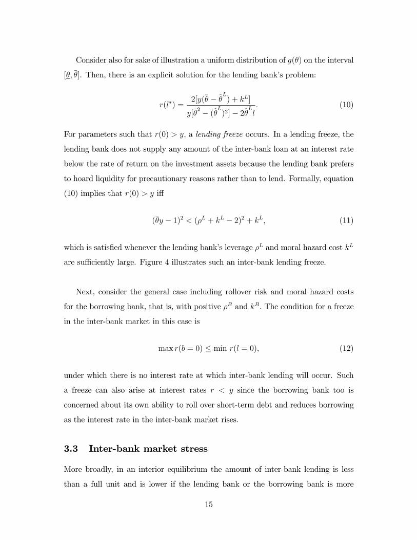
are su¢ ciently large. Figure 4 illustrates such an inter-bank lending freeze.
Next, consider the general case including rollover risk and moral hazard costs
for the borrowing bank, that is, with positive �B and kB: The condition for a freeze
in the inter-bank market in this case is
max r(b = 0) � min r(l = 0); (12)
under which there is no interest rate at which inter-bank lending will occur. Such
a freeze can also arise at interest rates r < y since the borrowing bank too is
concerned about its own ability to roll over short-term debt and reduces borrowing
as the interest rate in the inter-bank market rises.
3.3 Inter-bank market stress
More broadly, in an interior equilibrium the amount of inter-bank lending is less
than a full unit and is lower if the lending bank or the borrowing bank is more
15
2 2.1 2.2 2.3 2.4 2.5 2.6 2.7 2.8 2.9 30
0.1
0.2
0.3
0.4
0.5
0.6
0.7
0.8
0.9
1
Figure 4: Inter-bank Lending Freeze. Large leverage �L and moral hazard kL for thelending bank can cause a lending freeze in the inter-bank market, where the lendingbank does not supply any amount of the inter-bank loans at an interest rate belowthe return on the investment assets: l�(r � y) = 0. The borrowing bank neverborrows at r > y. Parameters are y = 2:4; �L = 1:5; �B = 0; kL = 0; kB = 0:5; and�~U [0:4; 1]:
leveraged or if their moral hazard problems are more severe. Neither bank risk-shifts
in equilibrium, but the possibility for risk-shifting in the future creates rollover risk
and leads the lending bank to hoard liquidity in advance and the borrowing bank
to reduce borrowing at high rates.
Proposition 1. Stress in inter-bank lending. The equilibrium inter-bank lend-
ing quantity l� is decreasing in the lending and borrowing banks� leverage �i and
moral hazard ki: dl�
d�i� 0 and dl�
dki� 0 for i = B;L:
It is also the case that as moral hazard or leverage increases for the lending bank,
the equilibrium inter-bank rate increases. Conversely, as the moral hazard problem
becomes more severe or leverage increases for the borrowing bank, its demand for
term borrowing decreases, which drives the inter-bank rate down.
Proposition 2. Stress in inter-bank rates. The equilibrium inter-bank rate r�
is increasing in the lending bank�s leverage �L and moral hazard kL, dr�
d�L� 0 and
16
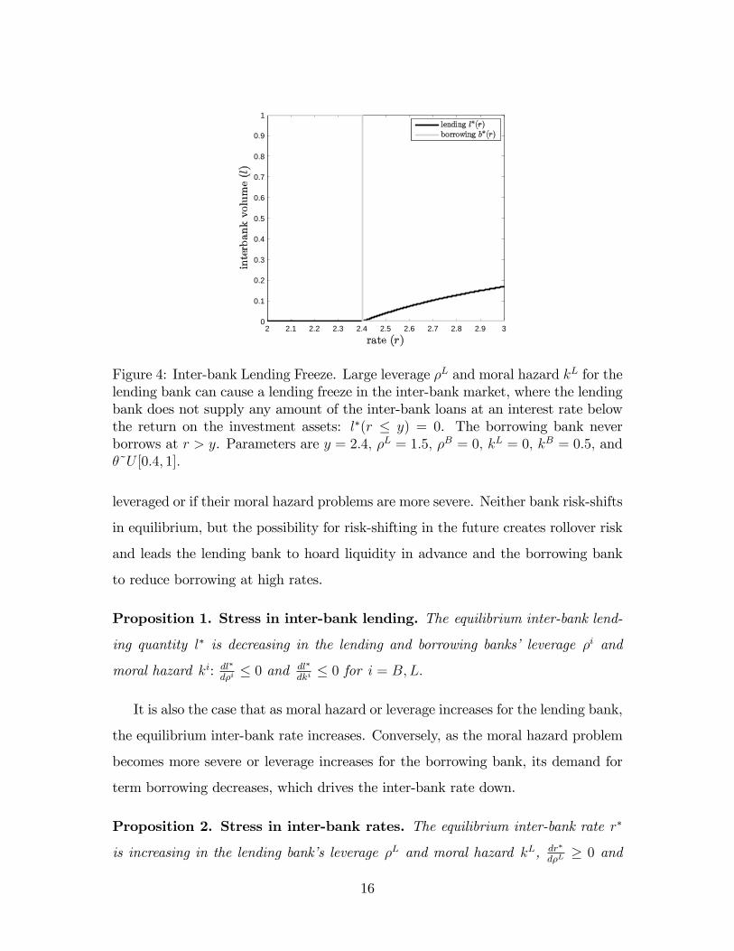
Figure 5: Equilibrium Lending Decreases in Banks�Moral Hazard. The �gure illus-trates the decrease in equilibrium lending l� with increasing moral hazard costs bythe lending bank, kL, and the borrowing bank, kB. Lending freezes entirely, l� = 0,for large enough moral hazard. Parameters are y = 2:4, �L = 1:3, and �B = 0,�~U [0:4; 1].
dr�
dkL� 0; and decreasing in the the borrowing bank�s leverage �B and moral hazard
kB, dr�
d�B� 0 and dr�
dkB� 0:
Figure 5 illustrates the sharp decrease in equilibrium lending with increasing
moral hazard costs (or illiquidity of the asset in place) kB and kL: Lending freezes
entirely for severe enough moral hazard, and similar illustrations are obtained for
large enough short-term leverage (�B and �L).
3.4 The alternative view: Counterparty risk
Consider again the contrast of our model with the traditional view of spreads in inter-
bank rates as based solely on counterparty (borrower) credit risk. With rollover risk
and induced precautionary desire to hold liquidity, the lender requires an interest
rate spread above the rate adjusted for the borrower�s credit risk: r > 1E[�]: The
lender requires this spread to compensate it for the risk of not being able to roll
17
over its short-term debt. This spread increases in the lender�s leverage, its asset
illiquidity, and uncertainty about its asset quality.
The increased spread charged by the lender induces the borrowing bank to reduce
its demand for inter-bank borrowing, as it faces its own rollover risk. At higher rates,
the borrower �nds it less worthwhile to make long-term investments at the expense of
taking on rollover risk and cuts back borrowing. Viewed another way, the borrower
too exhibits precautionary hoarding since it e¤ectively maintains more liquidity for
itself by borrowing less to fund long-term projects. As in the case of the lender, the
borrower�s precautionary behavior is stronger as its leverage, asset illiquidity, and
asset risk rise.
4 Empirical predictions and relevance of results
Our analytical results on hoarding of liquidity by banks and its e¤ect on inter-
bank rates are corroborated by empirical �ndings in the extant literature. Further,
the model also provides testable implications for teasing out borrower (demand)
and lender (supply) e¤ects in inter-bank markets. The precautionary liquidity view
provides ground for new policy insights. Moreover, the precautionary basis for
liquidity hoarding sits in contrast to the conventional basis for liquidity hoarding
based on strategic reasons. We discuss these points in turn.
4.1 Extant empirical evidence
The empirical literature on the inter-bank market predominantly examines the
overnight market, which we �rst examine. We then contrast this literature with
the emerging empirical literature on term inter-bank markets.
4.1.1 Liquidity hoarding and inter-bank markets
Acharya and Merrouche (2009) show empirically that during the �rst year of the
crisis (August 2007 to June 2008), some settlement banks in the United Kingdom
18
voluntarily revised upward their reserve balance targets with the Bank of England.
Such revisions followed critical dates of the crisis, such as the freeze in the asset-
backed commercial paper market of August 8, 2007, the collapse of Northern Rock
in mid-September 2007 and that of Bear Stearns in mid-March of 2008. In the cross-
section of banks, hoarding of liquidity �as measured by increases in reserve balance
targets �was greater for banks that had su¤ered greater equity losses in the crisis
(low � realization in the model) and had greater reliance on overnight wholesale
�nancing (greater �). They also document that this hoarding caused increases in
inter-bank lending rates for all other banks, in line with our Proposition 2.
Ashcraft, McAndrews and Skeie (2010) argue with similar evidence for the United
States during the crisis: to insure themselves against intraday liquidity shocks,
weaker banks facing heightened rollover risk held larger reserve balances. In partic-
ular, they report that banks sponsoring ABCP conduits witnessed increased pay-
ments shocks, and that greater payments shocks led to an increase in bank�s reserves.
In addition, banks appear to have responded to higher uncertainty about payments
during the crisis by becoming more reluctant to lend excess reserves to other banks
when reserves were high. These results are also suggestive of a precautionary de-
mand for liquidity and are entirely consistent with Lemma 3.
4.1.2 Overnight versus term inter-bank markets
Ashcraft, McAndrews and Skeie (2010) and Afonso, Kovner and Schoar (2010) argue
that overnight inter-bank lending in the fed funds and Eurodollar market increased
through much of the early crisis and held up well even after the Lehman bankruptcy.
However, Kuo, Skeie, Youle and Vickery (2011) suggest this was not the case for
maturities longer than overnight, especially one-month onwards. They argue that
inter-bank lending volumes generally fell during the heart of the crisis while term
spreads increased. Kuo, Skeie, Youle and Vickery (2011) claim a decline in the
maturity-structure (as illustrated in Figure 2), in line with our Proposition 1. The
claim of a decrease in term lending provides an explanation for the steady and even
19
increasing levels of overnight inter-bank lending: borrowing banks, facing height-
ened costs of term borrowing, shifted from term to overnight markets. Focusing
exclusively on the resilience of overnight inter-bank volumes can thus paint too rosy
a picture of inter-bank markets as it ignores the underlying stress felt in term inter-
bank markets. There is a potential caveat with the empirical evidence presented
in Section 4.1. Estimates of U.S. inter-bank activity are obtained by applying an
algorithm based on Fur�ne (1999) to Fedwire Funds data. Preliminary attempts by
NYFRB researchers (MaPS function) were unable to assess how large are the type
I and II errors generated by the algorithm.
4.2 Novel empirical predictions
Our model also o¤ers several new testable implications:
First, Lemma 3 shows that a bank�s lending rate for a particular maturity in the
inter-bank market increases with its own credit risk (e.g., balance-sheet leverage),
illiquidity of assets (e.g., holding of complex assets) and rollover risk (e.g., nature
of leverage �uninsured or wholesale deposits relative to insured or retail deposits),
controlling for the credit risk of the counterparties that borrow. More uniquely
to our model, Proposition 2 shows that a bank�s borrowing rate for a particular
maturity in the inter-bank market increases with credit risk, illiquidity and rollover
risk of the lender, controlling for the borrower�s own credit risk.16
Second, our model suggests tests that combine inter-bank rates and volumes. An
increase in the lender or borrower bank�s leverage drives down the bank�s lending
supply or borrowing demand for loans, respectively, which decreases the amount
of inter-bank lending (Proposition 1). An increase in the lender leverage, however,
increases the equilibrium inter-bank rate; in sharp contrast, an increase in the bor-
16In the model, we assume that banks act competitively, yet we recognize that inter-bank marketsare often segmented and that banks may not interact with all others. We model this by consid-ering individual borrower-lender pairs, in which both banks act as price-takers. An equilibriuminter-bank rate thus depends on the lender�s supply curve and hence the lender�s characteristics.Empirically, our model suggests that a rate at which a bank borrows depends on the characteristicsof the lending bank.
20
rower leverage decreases the equilibrium inter-bank rate (Proposition 2). A joint
analysis of inter-bank rates and volumes can thus help tease out the e¤ects of lender
supply versus borrower demand shifts. To the best of our knowledge, such joint
analysis of inter-bank rates and volumes with borrower and lender �xed e¤ects (or
characteristics) has not yet been conducted. All of these tests should hold if we
replaced borrower or lender leverage with asset illiquidity.
Third, our model suggests that an increase in the risk of asset-level shocks in-
creases term inter-bank rates, and reduces term inter-bank volumes. This is not
just due to an increase in the borrower�s credit risk. It is also due to an increase in
the rollover risk of the lender, as in Propositions 1 and 2. That is, term inter-bank
rates and volumes should contain an interaction e¤ect between risk (e.g., realized
or implied market volatility, as re�ected in the VIX) and both borrower and lender
leverage and rollover risk.17
Finally, our results indicate that measures of inter-bank market rates such as
LIBOR do not necessarily indicate the full breakdown that may occur in the inter-
bank market since there is no coincident provision of information on volumes. When
there is a complete breakdown of terms between some borrowers and lenders, the
inter-bank rate between some parties is not even well-de�ned. Rates based on actual
or quoted transactions may mask the breakdown in some parts of the market, un-
derstating the market average rate. Hence, measurement and reporting of volumes
in term inter-bank markets is crucial for understanding the stress and collapse in
these markets.18
17Fur�ne (2010) �nds that the LIBOR-OIS spread is related to VIX over time, supporting ourprediction, and results could be further tested by examining separate borrower and lender e¤ects.18Documenting transaction volumes that go with one, three and six month LIBOR rates is
potentially also important as they are used to index over $360 trillion of notional �nancial contracts,as estimated by the British Bankers�Association (BBA), ranging from interest rate swaps and otherderivatives to �oating-rate residential and commercial mortgages.
21
4.3 Policy conjectures
It is important to consider cases where the lending banks�precautionary demand for
liquidity may be excessive relative to its socially e¢ cient level. In turn, this would
suggest possible policy interventions to address excessive hoarding of liquidity by
highly leveraged banks. Is it desirable to have an unconditional (traditional) lender
of last resort (LOLR) in which a central bank provides liquidity to strong as well as
weak banks? Or would it be better to have a solvency-contingent LOLR in which
the central bank provides liquidity only to su¢ ciently strong banks? And should
there instead (or in addition) be a resolution authority that forces weak banks to
reduce their rollover risk? We conjecture that (i) a resolution authority to address
weak banks�excess leverage and rollover risk, and (ii) a solvency-contingent LOLR
by a central bank (that itself has lower credit and rollover risk than its banks), are
likely to be more e¤ective interventions than the traditional, unconditional LOLR.
Such welfare analysis can also help understand the impact of interventions that
were put in place during the crisis of 2007-09, such as the Term Auction Facility
(TAF) by the Federal Reserve for 28-day and later 84-day loans. We conjecture that
through these facilities, the Federal Reserve, acting as a relatively risk-free inter-
mediary, intermediated liquidity hoardings (reserves) of riskier banks to banks that
participated in the facilities. This intervention should have increased volumes of
lending to the real sector by the participating banks. Note that under the alterna-
tive view, that stress in inter-bank markets is caused purely by borrower credit-risk
problems, lending by central bank to banks at lower than market rates would ef-
fectively constitute a �bail out�of these banks and engender severe moral hazard.
However, a resolution authority to address weak banks�leverage and rollover risk
would be a robust intervention also under this alternative view.
4.4 Related literature
There is a growing body of theoretical literature on inter-bank markets. Our focus
is on the positive implications for the terms (quantity and interest rates) of liquid-
22
ity transfers in inter-bank markets when banks have short-term leverage and face
attendant agency problems. Hence, we restrict discussion of the related literature
on this theme.19
Rollover risk in our model induces banks to hold liquidity and raise inter-bank
rates or withdraw liquidity altogether from inter-bank markets. The literature has
also explored other motives for banks�desires to hold liquidity in crises. Acharya,
Shin and Yorulmazer (2008) derive a strategic motive for holding cash. When banks�
ability to raise external �nancing is low, they anticipate �re sales of assets by trou-
bled banks and as a result hoard liquidity and forego pro�table but illiquid invest-
ments. Diamond and Rajan (2009) also study long-term credit contraction that
operates through a channel of asset �re sales. During a crisis, banks delay asset
sales as part of their e¤orts to stay alive (a version of the risk-shifting problem).
In turn, high rates are required ex ante on term loans to the real sector. Finally,
Caballero and Krishnamurthy (2008) derive a propensity for �rms to hoard liquid
assets and reduce risk-sharing when there is Knightian uncertainty about their risks.
While these papers focus on aggregate liquidity shortages and strategic or behav-
ioral demand for liquidity by bank(er)s, we derive instead a precautionary demand
for liquidity by (weak) banks as contributing to heightened borrowing costs for (even
safe) banks. In a contemporary paper, Gale and Yorulmazer (2010) model both the
precautionary and the strategic motive for holding cash and show that banks may
hoard liquidity and lend less than the maximum possible amount, as in our model.
In our paper as well as in these other papers, a common theme is that the increase
in bank propensity to hold liquidity is in anticipation of crises, rather than (just)
upon their incidence. Diamond and Rajan (2005) also show how asset liquidations
19Goodfriend and King (1988) provide the benchmark result that with complete markets, inter-bank lending allows for the e¢ cient provision of lending among banks. To obtain deviations fromthis benchmark, Flannery (1996), Freixas and Jorge (2007), Freixas and Holthausen (2005) andHeider, Hoerova and Holthausen (2009) consider asymmetric information among banks, whereasDonaldson (1992) and Acharya, Gromb and Yorulmazer (2007) consider strategic behavior byrelationship-speci�c lenders. Skeie (2004, 2008) and Freixas, Martin and Skeie (2011) study thee¤ects of nominal contracts and monetary policy, respectively, on inter-bank markets and bankingfragility. Finally, Acharya, Gale and Yorulmazer (2008) show how rollover risk can arise uponadverse news even in absence of agency problems.
23
by some banks can ex post reduce the endogenous amount of aggregate liquid re-
sources available to even fundamentally healthy banks. The contagion in their paper
also operates through an increase in inter-bank market rates and results in a de-
crease in lending to the real sector. This is, however, an ex post contagion rather
than an ex ante one that is in anticipation of insolvency or rollover risk (as in our
model).
5 Concluding remarks
Stress and freezes in term inter-bank lending markets can be explained by rollover
risk of highly leveraged lenders and illiquidity of assets underlying term loans. We
showed that the term inter-bank lending rates and volumes are jointly determined,
re�ecting the precautionary demand for liquidity of lenders and aversion of borrowers
to trade at high rates of interest, both induced by their respective rollover risks. The
model�s implications are consistent with several empirical papers that study inter-
bank activity during �nancial crises.
The primary message from our analysis is that heightened rates and reduced
volumes in inter-bank markets should not necessarily be interpreted as being caused
solely by counterparty credit risk. These phenomena may re�ect the reluctance of
banks to give up liquidity for long maturities, or conversely, their precautionary
demand for liquidity.
References[1] V. V. Acharya, D. Gale, T. Yorulmazer, Rollover Risk and Market Freezes,
Journal of Finance, forthcoming (2008).
[2] V. V. Acharya, D. Gromb, T. Yorulmazer, Imperfect Competition in the Inter-bank Market for Liquidity as a Rationale for Central Banking, New York Uni-versity Stern School of Business working paper (2007).
[3] V. V. Acharya, O. Merrouche, Precautionary Hoarding of Liquidity and Inter-Bank Markets: Evidence from the Sub-prime Crisis, NYU Working Paper No.FIN-09-018 (2009).
24
[4] V. V. Acharya, P. Schnabl, G. Suarez, Securitization Without Risk Transfer,Working Paper, NYU-Stern (2009).
[5] V. V. Acharya, H. S. Shin, T. Yorulmazer, Crisis Resolution and Bank Liquidity,Review of Financial Studies, forthcoming (2008).
[6] V. V. Acharya, S. Viswanathan, Leverage, Moral Hazard and Liquidity, Journalof Finance 66 (2011) 99-138.
[7] G. Afonso, A. Kovner, A. Schoar, Stressed Not Frozen: The Federal FundsMarket in the Financial Crisis, Journal of Finance, forthcoming (2010).
[8] A. Ashcraft, J. McAndrews, D. Skeie, Precautionary Reserves and the Inter-bank Market, Journal of Money, Credit and Banking, forthcoming (2010).
[9] R. J. Caballero, A. Krishnamurthy, Collective Risk Management in a Flight toQuality Episode, Journal of Finance 63(5) (2008) 2195-2236.
[10] C. Calomiris, C. Kahn, The Role of Demandable Debt in Structuring OptimalBanking Arrangements, American Economic Review 81 (1991) 497�513.
[11] D. Diamond, Reputation Acquisition in Debt Markets, Journal of PoliticalEconomy 97(4) (1989) 828-862.
[12] D. Diamond, Debt Maturity Structure and Liquidity Risk, Quarterly Journalof Economics 106(3) (1991) 709-737.
[13] D. Diamond, P. Dybvig, Bank runs, deposit insurance, and liquidity, Journalof Political Economy 91(3) (1983) 401�419.
[14] D. Diamond, R. G. Rajan, Liquidity Risk, Liquidity Creation, and FinancialFragility: A Theory of Banking, Journal of Political Economy 109(2) (2001)287-327.
[15] D. Diamond, R. G Rajan, Liquidity Shortages and Banking Crises, Journal ofFinance 60 (2005).
[16] D. Diamond, R. G. Rajan, Fear of Fire Sales, Illiquidity Seeking and the CreditFreeze, Quarterly Journal of Economics, forthcoming (2009).
[17] G. R. Donaldson, Costly Liquidation, Inter-bank Trade, Bank Runs and Panics,Journal of Financial Intermediation 2 (1992) 59-85.
[18] M. Flannery, Financial Crises, Payments System Problems and Discount Win-dow Lending, Journal of Money, Credit and Banking 28 (1996) 804-824
[19] X. Freixas, J. Jorge, The Role of Inter-bank Markets in Monetary Policy: AModel with Rationing, Universitat Pompeu Fabra, mimeo (2007).
25
[20] X. Freixas, C. Holthausen, Interbank Market Integration under AsymmetricInformation, Review of Financial Studies 18 (2005) 459-90.
[21] X. Freixas, A. Martin, D. Skeie, Bank Liquidity, Interbank Markets and Mon-etary Policy, Review of Financial Studies, forthcoming (2011).
[22] C. Fur�ne, The Microstructure of the Federal Funds Market, Financial Markets,Institutions, and Instruments, 8(5) (1999) 24-44.
[23] C. Fur�ne, Exchange Traded Contracts During a Crisis, working paper (2010).
[24] D. Gale, T. Yorulmazer, Liquidity Hoarding, working paper (2010).
[25] M. Goodfriend, R. King, Financial Deregulation, Monetary Policy, and Cen-tral Banking, Federal Reserve Bank of Richmond Economic Review May/June(1988) 3-22.
[26] F. Heider, M. Hoerova, C. Holthausen, Liquidity Hoarding and Interbank Mar-ket Spreads: The Role of Counterparty Risk, European Banking Center Dis-cussion Paper No. 2009-11S (2009).
[27] M. Jensen, W. Meckling, Theory of the Firm: Managerial Behavior, AgencyCosts, and Capital Structure, Journal of Financial Economics 3 (1976) 305�360.
[28] D. Kuo, D. Skeie, T. Youle, J. Vickery, Identifying Term Wholesale Loans fromFedwire Payments Data, Federal Reserve Bank of New York, working paper(2011).
[29] J. McAndrews, A. Sarkar, Z. Wang, The E¤ect of the Term Auction Facility onthe London Inter-Bank O¤ered Rate, Federal Reserve Bank of New York Sta¤Reports No. 335 (2008).
[30] F. Michaud, C. Upper, What Drives Interbank Rates? Evidence from the LiborPanel, BIS Quarterly Review (2008).
[31] C. Schwarz, Mind the Gap: Disentangling Credit and Liquidity in Risk Spreads,University of Pennsylvania Wharton School of Business, working paper (2009).
[32] D. Skeie, Money and Modern Bank Runs, Princeton University, dissertation(2004).
[33] D. Skeie, Banking with Nominal Deposits and Inside Money, Journal of Finan-cial Intermediation 17 (2008) 562�84.
[34] J. Smith, The Term Structure of Money Market Spreads During the FinancialCrisis, New York University Stern School of Business, working paper (2010).
[35] J. Stiglitz, A. Weiss, Credit Rationing in Markets with Imperfect Information,American Economic Review 71 (1981) 393�410.
26
[36] J. Taylor, J. Williams, A Black Swan in the Money Market, NBER WorkingPaper No. 13943 (2008a).
[37] J. Taylor, J. Williams, Further Results on a Black Swan in the Money Market,Stanford University, working paper (2008b).
[38] J. van Kan, Use of LIBOR as an Index for Pricing Loans, Loan Market Asso-ciation LMA News, July (2010).
Appendix: Proofs
Analysis following Lemma 1. Consider the case where the lending bank can
fully pledge returns on the inter-bank loan, but the bank still faces the moral hazard
problem on the asset in place. The bank�s expected pro�t under no risk shifting is
�(y+ lr� fL) and under risk shifting is �LR(yL+ �lr� fL). The incentive constraint
not to risk shift is �fL � �(yL + lr) � kL: The individual rationality constraint for
the bank�s depositors is �L � (1 � l) � �fL: Together, the two constraints imply a
rollover constraint of
l � �yL � kL � �L + 11� �r :
For any lending rate r � 1�; an increased quantity of lending l relaxes the rollover
constraint. The bank prefers to lend its full liquidity. For parameters such that the
rollover constraint does not hold for l = 1 at a given lending rate r; the bank will
default at date 1 regardless of its inter-bank lending. The rate requirement for the
bank to to be able to roll over its debt is r � kL+�L
�� yL; which is increasing in the
severity of the bank�s moral hazard, kL:
In contrast, consider the case where the lending bank cannot pledge returns on
the inter-bank loan. Instead, suppose there is no moral hazard problem: kL = 0:
The rollover constraint is given by l � �y � �L + 1 and is tightened by increased
lending l: The bank does not lend its full liquidity if �L > �y: Moreover, for the case
of moral hazard case, when kL > 0; the quantity of lending declines linearly in kL;
as seen by the rollover constraint (6).
Assumption 1. We make two assumptions that ensure that the second order
condition is satis�ed. First, we assume a uniform distribution for g(�), which is
27
always su¢ cient to satisfy the condition needed for g0(�̂L) to be not too small.
This ensures that the lending bank has a minimal enough increase in its marginal
bankruptcy risk for marginal increases in its bankruptcy cuto¤ value �̂L. Second,
we assume large enough parameters for kL and �L relative to y such that
l >y
2r� 12(�L + kL � 1): (13)
Proof of Lemma 3. To study the second order condition of lender�s optimization
problem, note that
@2�L
@l2= �1
y(2�̂
Lr +
lr
y� 1)g(�̂L)� 1
y2(�̂Llr + kL)g0(�̂
L) (14)
= �g(�̂L)
y
"2�̂Lr +
lr
y� 1 + 1
y(�̂Llr + kL)
g0(�̂L)
g(�̂L)
#: (15)
For g0(�̂L) � 0; which is satis�ed by a uniform distribution for g(�); condition (13)
is su¢ cient for @2�L
@l2< 0. For l 2 [0; 1]; we can see that lending is increasing in r;
since
@2�L
@l@r=
Z ��
�̂L(l)
�g(�)d� � �̂L lyg(�̂
L) (16)
� �̂Lg(�̂
L)(1� l
y) (17)
� 0; (18)
where the last inequality holds since l � 1 < y: Lending is decreasing in �L; since
@2�L
@l@�= �(�̂Lr � 1)g(�̂L)1
y� lryg(�̂
L)1
y� 0; (19)
which is satis�ed by condition (13). Lending is also decreasing in kL; since
@2�L
@l@kL= �(�̂Lr � 1)g(�̂L)1
y� (1 + lr
y)g(�̂
L)1
y� 0; (20)
28
which is always satis�ed for l � 1 and r � y; the borrowing bank demand is never
positive for r > y, which can be excluded: �Proof of Proposition 2 and 3. In equilibrium, l�(r�; x) = b�(r�; x) and hencedl�
dx= db�
dxfor x 2 fkB; kL; �B; �Lg: Thus,
@l�
@x+@l�
@r�dr�
dx=@b�
@x+@b�
@r�dr�
dx; (21)
so we havedr�
dx= �
[@b�
@x� @l�
@x]
[ @b�
@r� �@l�
@r� ]: (22)
Now, @b�
@r� � 0 and@l�
@r� � 0; therefore sign(dr�
dx) = sign(@b
�
@x� @l�
@x). For x = kB; @l
�
@x= 0
and @b�
@x� 0; thus dr�
dkB� 0: For x = kL; @l
�
@x� 0 and @b�
@x� 0; thus dr�
dkL� 0: For
x = �B; @l�
@x= 0 and @b�
@x� 0; thus dr�
d�B� 0: For x = �L; @l�
@x� 0 and @b�
@x� 0; thus
dr�
d�L� 0:
Considerdl�
dx=@l�
@x+@l�
@r�dr�
dx: (23)
For x = kL; as shown above,
dr�
dkL=
@l�
@kL
@b�
@r� �@l�
@r�
; (24)
thereforedl�
dkL=@l�
@kL
"1�
@l�
@r�
@l�
@r� �@b�
@r�
#: (25)
Now@l�
@r�
@l�
@r� �@b�
@r�
� 1 (26)
as @b�
@r� � 0; hence, dl�
dkL� 0: Similarly, as @l�
@�L� 0; @l
�
@r� � 0, and dr�
d�L� 0; we have
dl�
d�L� 0: As @l�
@kB= 0; @l
�
@r� � 0, anddr�
dkB� 0; we have dl�
dkB� 0: Finally, as @l�
@�B� 0;
@l�
@r� � 0, anddr�
d�B� 0; we have dl�
d�B� 0: �
Appendix: Borrowing bank
29
At date 1, the borrowing bank needs to roll over short-term debt �B by issuing
new debt to depositors with a face amount fB due at date 2. Depositors of the
borrowing bank can verify whether the quantity (1 + b) invested in the asset has a
positive payo¤, but the cannot distinguish the level of the positive payo¤ or whether
the bank risk-shifts. The bank�s incentive constraint not to risk shift is


![Liquidity Hoarding in Financial Networks: The Role of ...downloads.hindawi.com/journals/complexity/2019/8436505.pdfcontagion [7]. Network approaches have proven useful for understanding](https://static.documents.pub/doc/80x56/60322ad543860e257a3c2944/liquidity-hoarding-in-financial-networks-the-role-of-contagion-7-network.jpg)


