• RESEARCH PAPER • April 2013 Vol.56 No.4: 1017–1028
doi: 10.1007/s11431-013-5153-1
A modified predictive control strategy of three-phase grid-connected converters with optimized action time sequence
SONG ZhanFeng1*, XIA ChangLiang1,2, LIU Tao1 & DONG Nan3
1 School of Electrical Engineering and Automation, Tianjin University, Tianjin 300072, China; 2 Tianjin Key Laboratory of Advanced Technology of Electrical Engineering and Energy, Tianjin Polytechnic University,
Tianjin 300387, China; 3 Beijing Electric Power Company, Beijing 100031, China
Received October 8, 2012; accepted January 15, 2013; published online February 23, 2013
Due to the excellent dynamic performance, the Finite Control Set Model Predictive Control has been widely used in various types of converters. However, when Finite Control Set Model Predictive Control is adopted, the switching frequency of con-verters varies significantly with system operating conditions. Consequently, constant-frequency predictive control strategy has been proposed. Two active voltage vectors and a zero voltage vector are selected within each sampling period. The action time sequence is then calculated. Due to the unsymmetrical distribution of current variation rates around zero, the calculated value of the voltage-vector action time will turn up negative. According to common sense, the voltage-vector action time is greater than or equal to zero. The action time is normally forced to zero whenever a negative value is predicted, resulting in the control failure and performance deterioration. To solve this problem, this paper proposes modified strategy. The modified strategy examines the action time calculated out. When negative action time comes out, the modified strategy reselects the active volt-age vector accordingly, instead of forcing the action time to be zero. Optimized action time sequence is further determined by minimizing the cost function. The effectiveness of the modified strategy is clearly verified by experimental tests, and analytical remarks are all founded in practical results.
converter, cost function, optimized action time sequence, negative action time
Citation: Song Z F, Xia C L, Liu T, et al. A modified predictive control strategy of three-phase grid-connected converters with optimized action time sequence. Sci China Tech Sci, 2013, 56: 10171028, doi: 10.1007/s11431-013-5153-1
1 Introduction
Three-phase grid-connected converters feature several ad-vantages, such as low current harmonic distortion, unity power factor operation, bidirectional power flow, and accu-rate control of the DC-side voltage. Three-phase grid-con- nected converters are widely used in a broad variety of ap-plications, including electrical drives, uninterrupted power supplies, and distributed power generations. Conventional control strategies are mostly based on the grid-voltage ori-
entation. Adjustment of currents is realized by adopting linear controllers in the synchronous rotating reference frame [1, 2]. For the design of conventional controllers, the converter is neglected, and a transfer function is obtained. Controllers are then designed based on this transfer function [3]. Model predictive control (MPC), a typical nonlinear control strategy, predicts the future system behavior based on the system model and the current state in each sampling period. The optimum control sequence is selected according to the cost function and the first element of the sequence is then applied. Different from traditional linear controllers, MPC adopts the online rolling optimiz-ation and can deal
1018 Song Z F, et al. Sci China Tech Sci April (2013) Vol.56 No.4
with various constraints. Therefore, it has been the research focus recently [4].
MPC is an extensive concept and can be divided into many kinds according to its operation principle and charac-teristics [5‒8]. One approach for implementing MPC for converters is known as Finite Control Set MPC (FCS-MPC). It makes use of the inherent discrete characteristics of the converter circuit, with full consideration of the finite switching states [9‒12]. Based on the current states and the discrete model, the future system behavior is predicted. The switch-ing state making the cost function minimum is then selected and applied [13, 14].
Due to the excellent dynamic performance, FCS-MPC has been widely used in various types of converters, such as matrix converters and multi-level converters [15‒17]. How-ever, the shortcomings of FCS-MPC regarding switching frequency restrict its further development. In each sampling period, the optimum voltage vector is selected by minimiz-ing the cost function. The selected vectors may be the same in adjacent two or more sampling periods. This indicates that the switching states during adjacent sampling periods may be unchanged. Consequently, the switching frequency varies significantly with system operating conditions, com-plicating the converter design. Filters need to be designed to eliminate broadband harmonics [18].
Therefore, some related literatures put forward some im-proved strategies. In ref. [19], a notch filter is embedded in the cost function to ensure constant switching frequency. However, similar to the conventional FCS-MPC algorithm, the control strategy proposed in ref. [19] selects only one voltage vector in a sampling period. Its steady-state control performance depends on the sampling frequency. In order to achieve better steady effect, higher sampling frequency needs to be adopted. In ref. [20], the constant-frequency MPC has been proposed. Two active voltage vectors and a zero voltage vector are selected within each sampling period. The action time sequence is then calculated by minimizing the cost function. This feature leads to the constant switch-ing frequency. However, it is found that the calculated value of the voltage-vector action time may be negative. The ac-tion time is normally forced to zero whenever a negative value is predicted, resulting in the control failure and per-formance deterioration. There is no report yet on detailed analysis and associated solutions with regard to the constant- frequency predictive current control.
To solve this problem, this paper proposes modified strategy. The modified strategy needs to examine the action time calculated. Whenever negative action time comes out, the modified strategy changes the active voltage vector ac-cordingly, instead of forcing the action time to be zero. The effectiveness of the modified strategy is clearly verified by experimental tests. The rest of this paper is organized as follows. In Section 2, the constant-frequency MPC is intro-duced briefly. In Section 3, influence of negative action time and improved predictive control are explained in detail.
Experimental results are displayed in Section 4. Finally, the conclusions are drawn in Section 5.
2 Model predictive control with constant fre-quency
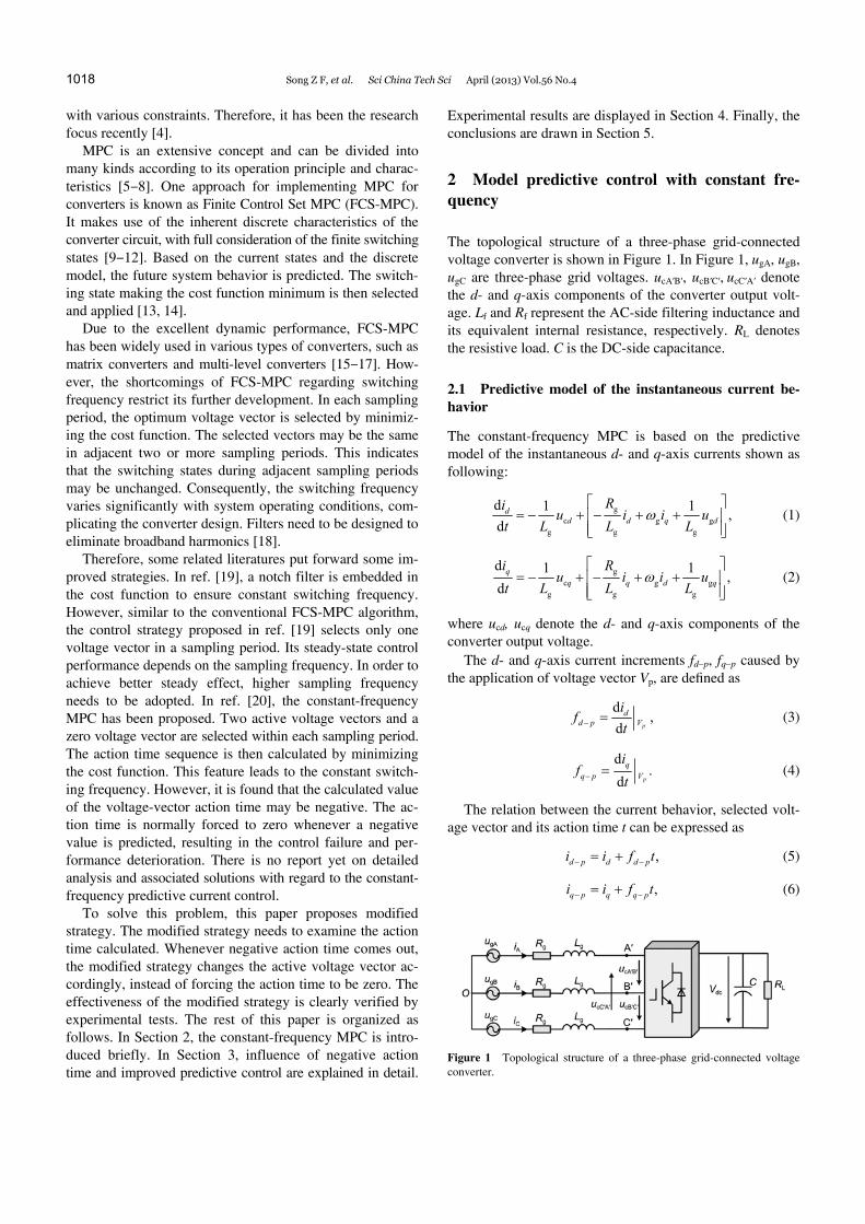
The topological structure of a three-phase grid-connected voltage converter is shown in Figure 1. In Figure 1, ugA, ugB, ugC are three-phase grid voltages. ucA′B′, ucB′C′, ucC′A′ denote the d- and q-axis components of the converter output volt-age. Lf and Rf represent the AC-side filtering inductance and its equivalent internal resistance, respectively. RL denotes the resistive load. C is the DC-side capacitance.
2.1 Predictive model of the instantaneous current be-havior
The constant-frequency MPC is based on the predictive model of the instantaneous d- and q-axis currents shown as following:
gc g g
g g g
d 1 1,
d
dd d q d
Riu i i u
t L L L (1)
gc g g
g g g
d 1 1,
d
qq q d q
i Ru i i u
t L L L (2)
where ucd, ucq denote the d- and q-axis components of the converter output voltage.
The d- and q-axis current increments fdp, fqp caused by the application of voltage vector Vp, are defined as
d
,d
p
dd p V
if
t (3)
d
.d
p
qq p V
if
t (4)
The relation between the current behavior, selected volt-age vector and its action time t can be expressed as
, d p d d pi i f t (5)
, q p q q pi i f t (6)
Figure 1 Topological structure of a three-phase grid-connected voltage converter.
Song Z F, et al. Sci China Tech Sci April (2013) Vol.56 No.4 1019
where idp and iqp are the predicted currents after the appli-cation of voltage vector Vp.
2.2 Voltage vectors sequence
Three voltage vectors including two active vectors and one zero vector are applied within each sampling period Ts. The two active voltage vectors should be selected in order to minimize current ripples. The smallest current ripples can be achieved by application sequence of neighboring voltage vectors. Based on the location of grid voltage vector, the two nearest-located active vectors Vm and Vn are selected, where m and n denote the selected vector numbers (m, n∈[1, 6]). These two active vectors will be used together with zero vectors V0,7. The selected voltage vectors and their sequences in different sectors are shown in Table 1.
When three voltage vectors are selected within one sam-pling period and symmetrical vectors application is to be achieved, the d- and q-axis current behaviors within a sam-pling period of Ts can be depicted as Figure 2.
Based on Figure 2, eqs. (5) and (6) can be rewritten as
01 0
2 1
3 2
4 3 0 0
5 4
6 5
07 6 0
,2
,,,,,
;2
d p d d
d p d p d m m
d p d p d n n
d p d p d
d p d p d n n
d p d p d m m
d p d p d
ti i f
i i f ti i f ti i f ti i f ti i f t
ti i f
(7)
01 0
2 1
3 2
4 3 0 0
5 4
6 5
07 6 0
,2
,,,,,
,2
q p q q
q p q p q m m
q p q p q n n
q p q p q
q p q p q n n
q p q p q m m
q p q p q
ti i f
i i f ti i f ti i f ti i f ti i f t
ti i f
(8)
s 02( ), m nT t t t (9)
where tm, tn are action time for two active voltage vector Vm
Table 1 Selected voltage vectors and their sequences
Sector Vm Vn Voltage vector sequence
I V1 V2 V0 V1 V2 V7 V2 V1 V0
II V2 V3 V0 V3 V2 V7 V2 V3 V0
III V3 V4 V0 V3 V4 V7 V4 V3 V0
IV V4 V5 V0 V5 V4 V7 V4 V5 V0
V V5 V6 V0 V5 V6 V7 V6 V5 V0
VI V6 V1 V0 V1 V6 V7 V6 V1 V0
and Vn, respectively. t0 is zero voltage vector action time. Eqs. (7), (8) and (9) can be simplified to
0 02 2 2 , d p d d d m m d n ni i f t f t f t (10)
0 02 2 2 . q p q q q m m q n ni i f t f t f t (11)
State-space representation of current behaviors within a sampling period of Ts is shown in Figure 3.
2.3 Calculation of voltage vector action time based on cost function
Similar to FCS-MPC and direct power control mentioned in ref. [21], the constant-frequency MPC employs a prediction horizon of one sampling period, which is particularly attrac-tive due to the simplicity of implementation. For a predic-tion horizon of one sampling period, the predicted current values at the end of each sampling period are expected to be id_ref and iq_ref, respectively. The d- and q-axis current errors at the end of each sampling period can thus be expressed as
Figure 2 d- and q-axis current behaviors within a sampling period of Ts.
Figure 3 State-space representation of current behaviors within a sam-pling period of Ts.
1020 Song Z F, et al. Sci China Tech Sci April (2013) Vol.56 No.4
s_err _ref 02 ,
2
d d d d m m d n n d m n
Ti i i f t f t f t t
(12)
s_err _ref 02 .
2
q q q q m m q n n q m n
Ti i i f t f t f t t
(13)
To minimize current errors, least square optimization method is introduced to construct the cost function. The cost function J is defined as a sum of squared errors
2 2_err _err
2
s_ref 0
2
s_ref 0
22
2 .2
d q
d d d m m d n n d m n
q q q m m q n n q m n
J i i
Ti i f t f t f t t
Ti i f t f t f t t
(14)
The action time tm, tn, t0, which can minimize cost func-tion value J during one sampling period, will be chosen for implementation. tm, tn, t0 satisfy the following minimum value condition
0,
m
J
t (15)
0.
n
J
t (16)
3 Influence of negative action time and im-proved predictive control
As mentioned in the previous sections, two active voltage vectors and a zero voltage vector are selected within each sampling period. The action time sequence tm, tn, t0 is then calculated by minimizing the cost function (14). It is found that the calculated action time may be negative in some sit-uations. According to common sense, the action time of voltage vectors is greater than or equal to zero. Consequently, the action time is normally forced to be zero whenever a negative value is predicted. This strategy is denoted as Method A in this paper. Obviously, the actual action time adopted in Method A is different from the optimal value. This will result in the deterioration of current performance, which is clearly visible in the experiment results shown below. The cause of the negative action time and its influ-ences will be analyzed below.
Figure 4 shows the set of active voltage vectors and mapping of the segments related to the line-voltage vector location. For clarity and better understanding, 6 original sectors are further divided into 12 subsections.
Within a fixed sector, 8 voltage vectors V0‒V7 produce
Figure 4 Set of active voltage vectors and mapping of the segments related to the line-voltage vector location.
different values in currents variation rates. Figure 5 demon-strates variation rates of the d- and q-axis currents when the system operates at rated power with unity power factor. The converter parameters will be given in Section 4. The ordi-nates of Figures 5(a) and 5(b) represent variation rates of the d- and q-axis currents, respectively. Positive ordinate values indicate the increase of currents. Otherwise, currents are decreased.
It is clearly visible that the d- and q-axis current variation rates are asymmetrically distributed around zero. The d-axis current variation rates locate between 5 kA s1 and 25 kA s1. This indicates that, in most cases, active voltage vectors V1‒V6 lead to the increase of d-axis current. Meanwhile, the action of two zero vectors V0,7 increases the d-axis current throughout each sampling period. With regard to the q-axis current, its variation rates locate between 20 kA s1 and 10 kA s1. This indicates that, in most cases, active voltage vectors V1‒V6 result in the decrease of the q-axis current. Meanwhile, the application of zero vectors V0,7 decreases the q-axis current throughout each sampling period.
Due to the unsymmetrical distribution of current varia-tion rates around zero, the calculated value of the voltage- vector action time will turn up negative, resulting in per-formance deterioration. Taking Sector I-① for example, V1, V2, V0,7 are to be selected when the line-voltage vector is located in this sector. It is clearly visible in Figure 5(b) that, the variation rate of the q-axis current resulting from V1 increases with the grid-voltage phase, from negative value to zero, and further to positive value. However, the variation rate of q-axis current corresponding to V2 and V0,7 retains negative throughout the whole sampling period. The above analysis indicates that, with the increase of grid-voltage phase, the application of V1 firstly results in the decrease of q-axis current and then its increase. And the action of V2,
Song Z F, et al. Sci China Tech Sci April (2013) Vol.56 No.4 1021
Figure 5 Effect of 8 voltage vectors on variation rates of d- and q-axis currents. (a) Variation rates of d-axis current; (b) variation rates of q-axis current.
V0,7 will always decrease the q-axis current. Similarly, for the d-axis current, when the grid-voltage vector locates in Sector I-①,with the increase of grid-voltage phase, the ap-plication of V2 firstly results in the increase of the q-axis current and then its decrease. The action of V1 will always decrease the q-axis current, and the action of zero vectors V0,7 will increase it all the time.
It can be inferred that, in Sector I-①, V1, V2, V0,7 can re-alize the flexible control of the d-axis current. The reason is that, throughout the whole sector, there always exist voltage vectors which can increase the d-axis current as well as voltage vectors which result in its decrease. However, this is not the case for the q-axis current. When the grid-voltage vector locates in the first half of Sector I-①, the vectors V1, V2, V0,7 all lead to the decrease of the q-axis current. This means that, no matter how long the action time of these vectors is, precise control of the q-axis current cannot be realized. In this situation, the voltage-vector action time calculated by the cost function will be negative.
For clarity and better understanding, variations of the d- and q-axis currents when the grid voltage is located at dif-
ferent sectors are shown in Tables 2 and 3, respectively. In these tables, indicates decrease of currents while de-notes increase of currents.
It is clearly visible in Table 3 that, in the first half of each Sector ①, three selected voltage vectors all lead to the de-crease of the q-axis current. In this situation, when the cost function is adopted to calculate the action time, the volt-age-vector action time will be negative, as shown in Figure 6. This negative value is forced to be zero in Method A, which will surely result in the control failure and perfor-mance deterioration of the system. This will be clearly clar-ified in the following experimental investigations.
To solve this problem, an improved strategy called Method B is proposed in this paper. Whenever negative action time comes out, Method B reselects the active volt-age vector accordingly, instead of forcing the action time to
Table 2 Variation of d-axis currents when the grid voltage is located at different sectors
Sector Voltage vector and its influence
I ① V1 V2 V0,7
② V1 V2 V0,7
II ① V2 V3 V0,7
② V2 V3 V0,7
III ① V3 V4 V0,7
② V3 V4 V0,7
IV ① V4 V5 V0,7
② V4 V5 V0,7
V ① V5 V6 V0,7
② V5 V6 V0,7
VI ① V6 V1 V0,7
② V6 V1 V0,7
Table 3 Variation of q-axis currents when the grid voltage is located at different sectors
Sector Voltage vector and its influence
I ① V1 V2 V0,7
② V1 V2 V0,7
II ① V2 V3 V0,7
② V2 V3 V0,7
III ① V3 V4 V0,7
② V3 V4 V0,7
IV ① V4 V5 V0,7
② V4 V5 V0,7
V ① V5 V6 V0,7
② V5 V6 V0,7
VI ① V6 V1 V0,7
② V6 V1 V0,7
1022 Song Z F, et al. Sci China Tech Sci April (2013) Vol.56 No.4
Figure 6 Regional location when the calculated time value is negative. (a) Regional location and variation of q-axis current; (b) regional location and variation of d-axis current. , The calculated duration time becomes negative; , the calculated duration time stays positive.
be zero. Taking the grid-voltage vector located in Sector I-① for example, it is demonstrated in Figure 6 and Table 3 that, the action time tn corresponding to the voltage vector V2 can be negative. Similar to the direct power control strategy mentioned in ref. [21], the most direct method is that the opposite vector V5 corresponding to V2 in Figure 4, is selected. A new combination V1, V5, V0,7 is thus con-structed to replace the former combination V1, V2, V0,7.
With regard to the new combination, V5 keeps the q-axis current increasing in the whole Sector I-①. V1 firstly de-creases the q-axis current then increases it, while the action of zero vectors V0,7 decreases it all the time. Therefore, the new combination V1, V5, V0,7 can realize flexible control of the q-axis current.
However, it is clearly visible in Figure 4 that V1 and V5 are non-adjacent vectors. Selection of non-adjacent vectors may cause large current ripples [22]. It can be observed in Figure 6 that the effect of V6 on current variation is similar to that of V5 in Sector I-①. V1 and V5 both lead to the in-crease of the q-axis current. Besides, V6 and V1 are adjacent vectors. Therefore, V6, instead of V5, is selected. A new combination V1, V6, V0,7 is thus constructed, which can also realize flexible control of the q-axis current. The improved voltage sequence for Method B in different sectors is shown in Table 4. The effectiveness of Method B is to be con-firmed by experimental results shown in the next section.
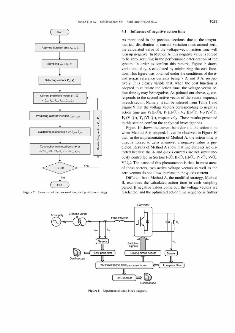
The corresponding flowchart of the proposed modified predictive control strategy is given in Figure 7. Differing from Method A, Method B needs to examine the calculated action time. If the calculated action time is positive, the al-gorithm procedure continues to run. If negative value comes out, the voltage vector needs to be reselected according to Table 3, and the optimized action time sequence is further determined by minimizing the cost function.
4 Experimental investigations
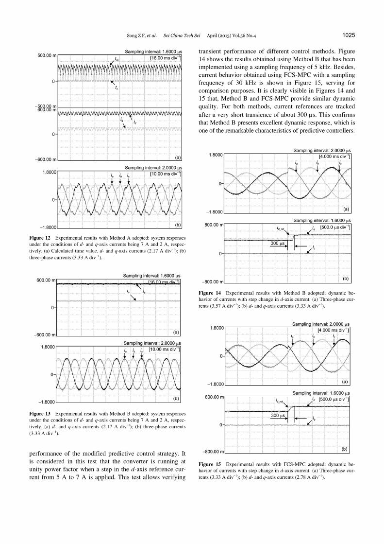
For the experimental verification of the modified predictive control strategy, an experimental platform for three-phase grid-connected voltage converter with power devices IGBT FGA40N120D was built and tested, as shown in Figure 8. The complete system was connected to the utility grid through a three-phase variac. An input filter inductor was adopted to attenuate switching harmonics. The digital platform based on TI company’s TMS320F28335 DSP was used for the control strategy. The rated power of the experimental plat-form is 0.5 kW. The grid line-to-line voltage is 95 V. The filter inductance and its equivalent resistance are 8 mH and 0.1 , respectively. The DC-link voltage is 160 V, and the DC-link capacitor is 2200 F. The experimental results were recorded by a YOKOGAWA digital storage oscillo-scope DLM2024.
Song Z F, et al. Sci China Tech Sci April (2013) Vol.56 No.4 1023
Figure 7 Flowchart of the proposed modified predictive strategy.
4.1 Influence of negative action time
As mentioned in the precious sections, due to the unsym-metrical distribution of current variation rates around zero, the calculated value of the voltage-vector action time will turn up negative. In Method A, this negative value is forced to be zero, resulting in the performance deterioration of the system. In order to confirm this remark, Figure 9 shows variations of tm, tn calculated by minimizing the cost func-tion. This figure was obtained under the conditions of the d- and q-axis reference currents being 7 A and 0 A, respec-tively. It is clearly visible that, when the cost function is adopted to calculate the action time, the voltage-vector ac-tion time tn may be negative. As pointed out above, tn cor-responds to the second active vector of the vector sequence in each sector. Namely, it can be inferred from Table 1 and Figure 9 that the voltage vectors corresponding to negative action time are V2 (I-①), V3 (II-①), V4 (III-①), V5 (IV-①), V6 (V-①), V1 (VI-①), respectively. These results presented in this section confirm the analytical investigations.
Figure 10 shows the current behavior and the action time when Method A is adopted. It can be observed in Figure 10 that, in the implementation of Method A, the action time is directly forced to zero whenever a negative value is pre-dicted. Results of Method A show that line currents are dis-torted because the d- and q-axis currents are not simultane-ously controlled in Sectors I-①, II-①, III-①, IV-①, V-①, VI-①. The cause of this phenomenon is that, in most areas of these sectors, two active voltage vectors as well as the zero vectors do not allow increase in the q-axis current.
Different from Method A, the modified strategy, Method B, examines the calculated action time in each sampling period. If negative values come out, the voltage vectors are reselected, and the optimized action time sequence is further
Figure 8 Experimental setup block diagram.
1024 Song Z F, et al. Sci China Tech Sci April (2013) Vol.56 No.4
Figure 9 Experimental results: calculated time value and the corre-sponding sector number under the conditions of d- and q-axis currents being 7 A and 2 A, respectively.
Figure 10 Experimental results with Method A adopted: system re-sponses under the conditions of d- and q-axis currents being 5 A and 0 A, respectively. (a) Calculated time value, d- and q-axis currents (2.17 A div1); (b) three-phase currents (3.57 A div1); (c) spectrum analysis for A-phase current.
determined by the cost function. In order to verify the effec-tiveness of the modified control scheme, Figure 11 shows system responses under the conditions of the d- and q-axis currents being 5 A and 0 A, respectively. It is clearly visible that currents waveforms of Method B are more sinusoidal than those of Method A, indicating that Method B allows smooth and simultaneous control of the d- and q-axis cur-rent in all sectors. The d-axis current is maintained constant and very close to the reference value and the q-axis current is zero on average in all sectors. As a result, three-phase currents are very close to sine wave. The effectiveness of the modified strategy is clearly verified, and all previous remarks are founded in practical results.
Similar results are further derived and confirmed by ex-perimental results as shown in Figure 12 under the condi-tions of the d- and q-axis currents being 7 A and 2 A, re-spectively. When comparing this result with the one shown in Figure 13, it is clear that the implementation of Method B enhances the behavior of the control, allowing for good control of currents.
4.2 Current reference tracking
This set of experiments deals with current reference tracking
Figure 11 Experimental results with Method B adopted: system responses under the conditions of d- and q-axis currents being 5 A and 0 A, respec-tively. (a) d- and q-axis currents (2.17 A div1); (b) three-phase currents (3.33 A div1). (c) spectrum analysis for A-phase current.
Song Z F, et al. Sci China Tech Sci April (2013) Vol.56 No.4 1025
Figure 12 Experimental results with Method A adopted: system responses under the conditions of d- and q-axis currents being 7 A and 2 A, respec-tively. (a) Calculated time value, d- and q-axis currents (2.17 A div1); (b) three-phase currents (3.33 A div1).
Figure 13 Experimental results with Method B adopted: system responses under the conditions of d- and q-axis currents being 7 A and 2 A, respec-tively. (a) d- and q-axis currents (2.17 A div1); (b) three-phase currents (3.33 A div1).
performance of the modified predictive control strategy. It is considered in this test that the converter is running at unity power factor when a step in the d-axis reference cur-rent from 5 A to 7 A is applied. This test allows verifying
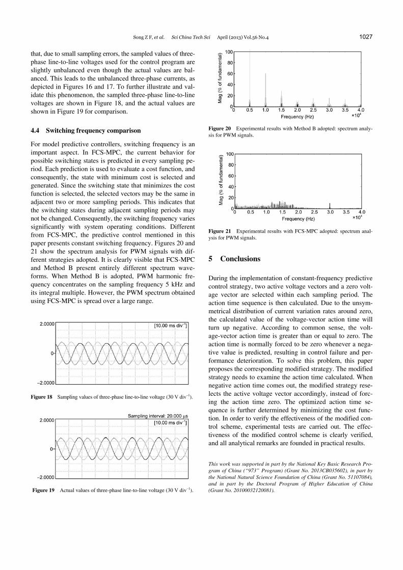
transient performance of different control methods. Figure 14 shows the results obtained using Method B that has been implemented using a sampling frequency of 5 kHz. Besides, current behavior obtained using FCS-MPC with a sampling frequency of 30 kHz is shown in Figure 15, serving for comparison purposes. It is clearly visible in Figures 14 and 15 that, Method B and FCS-MPC provide similar dynamic quality. For both methods, current references are tracked after a very short transience of about 300 s. This confirms that Method B presents excellent dynamic response, which is one of the remarkable characteristics of predictive controllers.
Figure 14 Experimental results with Method B adopted: dynamic be-havior of currents with step change in d-axis current. (a) Three-phase cur-rents (3.57 A div1); (b) d- and q-axis currents (3.33 A div1).
Figure 15 Experimental results with FCS-MPC adopted: dynamic be-havior of currents with step change in d-axis current. (a) Three-phase cur-rents (3.33 A div1); (b) d- and q-axis currents (2.78 A div1).
1026 Song Z F, et al. Sci China Tech Sci April (2013) Vol.56 No.4
It should be noted that in this set of experiments, the sampling frequency of Method B is 5 kHz, while that of FCS-MPC is 30 kHz. This indicates that, compared with FCS-MPC, Method B proposed in this paper allows for good control of currents with lower sampling frequency.
4.3 Steady-state performance
Due to the excellent dynamic performance, FCS-MPC has been widely used. However, its steady-state performance is to be improved. When FCS-MPC is adopted, the future sys-tem behavior is predicted based on the current states and the discrete model. The switching state making the cost func-tion minimum is then selected and applied. Since only one switching state is selected, the controller ensures minimal error but not zero steady error at the end of each sampling period [23]. Nevertheless, this is not the case for Method B. In each sampling period, Method B selects three voltage vectors within each sampling period, and calculates the op-timized action time sequence, which minimizes cost func-tion defined as a sum of the squared current errors. This ensures good steady-state performance as well as constant switching frequency. To verify the steady-state performance of Method B, detailed behaviors of the d- and q-axis cur-rents are shown in Figure 16, where the steady-state behavior
Figure 16 Experimental results with Method B adopted: steady-state behavior of currents under the conditions of d- and q-axis currents being 7 A and 2 A, respectively. (a) Three-phase currents (3.33 A div1); (b) d- and q-axis currents (2.89 A div1); (c) spectrum analysis for A-phase current.
is shown for a reference of 7 A and 2 A. For comparison, experimental results with FCS-MPC adopted are shown in Figure 17.
As it can be observed, the d- and q-axis currents trajecto-ries obtained using Method B is maintained constant and close to the reference values, while those obtained using FCS-MPC present small ripples. Comparisons of current spectrum with different controllers also verify the excellent steady-state performance of Method B.
However, it is demonstrated in Figure 16 that when the modified predictive strategy is adopted, three-phase currents are slightly unbalanced. This phenomenon can also be ob-served in Figure 17 with FCS-MPC adopted. This is due to sampling errors of line-to-line voltages Vab, Vbc, and Vca. During the sampling process, Vab and Vbc are often directly obtained through voltage sensors, while Vca is calculated as Vca=VabVbc. If small sampling errors are denoted as Vab and Vbc, respectively, the sampled values for Vab and Vbc
can be represented by Vab+Vab and Vbc+Vbc. The calculated value of Vca can thus be represented as VabVabVbcVbc= VcaVabVbc. Therefore, the sampled values of line-to- line voltages used for the control program are Vab+Vab, Vbc+Vbc, and VcaVabVbc, respectively. This indicates
Figure 17 Experimental results with FCS-MPC adopted: steady-state behavior of currents under the conditions of d- and q-axis currents being 7 A and 2 A, respectively. (a) Three-phase currents (3.33 A div1); (b) d- and q-axis currents (2.89 A div1); (c) spectrum analysis for A-phase current.
Song Z F, et al. Sci China Tech Sci April (2013) Vol.56 No.4 1027
that, due to small sampling errors, the sampled values of three- phase line-to-line voltages used for the control program are slightly unbalanced even though the actual values are bal-anced. This leads to the unbalanced three-phase currents, as depicted in Figures 16 and 17. To further illustrate and val-idate this phenomenon, the sampled three-phase line-to-line voltages are shown in Figure 18, and the actual values are shown in Figure 19 for comparison.
4.4 Switching frequency comparison
For model predictive controllers, switching frequency is an important aspect. In FCS-MPC, the current behavior for possible switching states is predicted in every sampling pe-riod. Each prediction is used to evaluate a cost function, and consequently, the state with minimum cost is selected and generated. Since the switching state that minimizes the cost function is selected, the selected vectors may be the same in adjacent two or more sampling periods. This indicates that the switching states during adjacent sampling periods may not be changed. Consequently, the switching frequency varies significantly with system operating conditions. Different from FCS-MPC, the predictive control mentioned in this paper presents constant switching frequency. Figures 20 and 21 show the spectrum analysis for PWM signals with dif-ferent strategies adopted. It is clearly visible that FCS-MPC and Method B present entirely different spectrum wave-forms. When Method B is adopted, PWM harmonic fre-quency concentrates on the sampling frequency 5 kHz and its integral multiple. However, the PWM spectrum obtained using FCS-MPC is spread over a large range.
Figure 18 Sampling values of three-phase line-to-line voltage (30 V div1).
Figure 19 Actual values of three-phase line-to-line voltage (30 V div1).
Figure 20 Experimental results with Method B adopted: spectrum analy-sis for PWM signals.
Figure 21 Experimental results with FCS-MPC adopted: spectrum anal-ysis for PWM signals.
5 Conclusions
During the implementation of constant-frequency predictive control strategy, two active voltage vectors and a zero volt-age vector are selected within each sampling period. The action time sequence is then calculated. Due to the unsym-metrical distribution of current variation rates around zero, the calculated value of the voltage-vector action time will turn up negative. According to common sense, the volt-age-vector action time is greater than or equal to zero. The action time is normally forced to be zero whenever a nega-tive value is predicted, resulting in control failure and per-formance deterioration. To solve this problem, this paper proposes the corresponding modified strategy. The modified strategy needs to examine the action time calculated. When negative action time comes out, the modified strategy rese-lects the active voltage vector accordingly, instead of forc-ing the action time zero. The optimized action time se-quence is further determined by minimizing the cost func-tion. In order to verify the effectiveness of the modified con-trol scheme, experimental tests are carried out. The effec-tiveness of the modified control scheme is clearly verified, and all analytical remarks are founded in practical results.
This work was supported in part by the National Key Basic Research Pro-gram of China (“973” Program) (Grant No. 2013CB035602), in part by the National Natural Science Foundation of China (Grant No. 51107084), and in part by the Doctoral Program of Higher Education of China (Grant No. 20100032120081).
1028 Song Z F, et al. Sci China Tech Sci April (2013) Vol.56 No.4
1 Song Z, Xia C L, Shi T N. Assessing transient response of DFIG based wind turbines during voltage dips regarding main flux satura-tion and rotor deep-bar effect. Appl Energ, 2010, 87(10): 3283–3293
2 Mohamed Y A I. Mitigation of dynamic, unbalanced, and harmonic voltage disturbances using grid-connected inverters with LCL filter. IEEE T Ind Electron, 2011, 58(9): 3914–3924
3 Kouro S, Cortés P, Vargas R, et al. Model predictive control—A simple and powerful method to control power converters. IEEE T Ind Electron, 2009, 56(6): 1826–1838
4 Aswani A, Master N, Taneja J, et al. Reducing transient and steady state electricity consumption in HVAC using learning-based mod-el-predictive control. IEEE Proc, 2012, 100(1): 240–253
5 Barrero F, Prieto J, Levi E, et al. An enhanced predictive current con-trol method for asymmetrical six-phase motor drives. IEEE T Ind Electron, 2011, 58(8): 3242–3252
6 Geyer T. Computationally efficient model predictive direct torque control. IEEE T Power Electron, 2011, 26(10): 2804–2816
7 Geyer T, Papafotiou G, Morari M. Model predictive direct torque control—Part I: concept, algorithm, and analysis. IEEE T Ind Elec-tron, 56(6): 1894–1905
8 Papafotiou G, Kley J, Papadopoulos K G, et al. Model predictive di-rect torque control—Part II: implementation and experimental evalu-ation. IEEE T Ind Electron, 2009, 56(6): 1906–1915
9 Lee K, Park B, Kim R, et al. Robust predictive current controller based on a disturbance estimator in a three-phase grid-connected in-verter. IEEE T Power Electron, 2012, 27(1): 276–283
10 Landsmann P, Kennel R. Saliency-based sensorless predictive torque control with reduced torque ripple. IEEE T Power Electron, 2012, 27(10): 4311–4320
11 Perez M A, Rodriguez J, Fuentes E J, et al. Predictive control of AC–AC modular multilevel converters. IEEE T Ind Electron, 2012, 59(7): 2832–2839
12 Duran M J, Prieto J, Barrero F, et al. Predictive current control of du-al three-phase drives using restrained search techniques. IEEE T Ind
Electron, 2011, 58(8): 3253–3263 13 Quevedo D E, Aguilera R P, Pérez M A, et al. Model predictive con-
trol of an AFE rectifier with dynamic references. IEEE T Power Electron, 2012, 27(7): 3128–3136
14 Cortes P, Rodriguez J, Silva C, et al. Delay compensation in model predictive current control of a three-phase inverter. IEEE T Ind Elec-tron, 2012, 59(2): 1323–1325
15 Davari S A, Khaburi D A, Kennel R. An improved FCS–MPC algo-rithm for an induction motor with an imposed optimized weighting factor. IEEE T Power Electron, 2012, 27(3): 1540–1551
16 Rodríguez J, Kennel R M, Espinoza J R, et al. High-performance control strategies for electrical drives: an experimental assessment. IEEE T Ind Electron, 2012, 59(2): 812–820
17 Errouissi R, Ouhrouche M, Chen W, et al. Robust nonlinear predictive controller for permanent-magnet synchronous motors with an optimized cost function. IEEE T Ind Electron, 2012, 59(7): 2849–2858
18 Ramchand R, Gopakumar K, Patel C, et al. Online computation of hysteresis boundary for constant switching frequency current-error space-vector-based hysteresis controller for VSI-fed IM drives. IEEE T Power Electron, 2012, 27(3): 1521–1529
19 Cortes P, Rodriguez J, Quevedo D E, et al. Predictive current control strategy with imposed load current spectrum. IEEE T Power Electron, 2008, 23(2): 612-618
20 Xia C, Wang M, Song Z F, et al. Robust model predictive current control of three-phase voltage source PWM rectifier with online dis-turbance observation. IEEE T Ind Inf, 2012, 8(3): 459–471
21 Hu J, Zhu Z. Investigation on switching patterns of direct power con-trol strategies for grid-connected DC–AC converters based on power variation rates. IEEE T Power Electron, 2011, 26(12): 3582–3598
22 Antoniewicz P. Predictive control of Three Phase AC/DC Converters. Ph D Dissertation. Warsaw: Warsaw University of Technology, 2009
23 Lezana P, Aguilera R, Quevedo D E. Steady-state issues with finite control set model predictive control. Proc IEEE Annu Conf Ind Elec-tron Soc, 2009. 1776–1781