A Möbius-Invariant Power Diagram and Its Applications to Soap … · Discrete Comput Geom (2014)...

Discrete Comput Geom (2014) 52:515–550DOI 10.1007/s00454-014-9627-0

A Möbius-Invariant Power Diagramand Its Applications to Soap Bubblesand Planar Lombardi Drawing

David Eppstein

Received: 10 September 2013 / Revised: 1 March 2014 / Accepted: 8 July 2014 /Published online: 5 September 2014© Springer Science+Business Media New York 2014

Abstract We use three-dimensional hyperbolic geometry to define a form of powerdiagram for systems of circles in the plane that is invariant under Möbius transfor-mations. By applying this construction to circle packings derived from the Koebe–Andreev–Thurston circle packing theorem, we show that every planar graph of max-imum degree three has a planar Lombardi drawing (a drawing in which the edgesare drawn as circular arcs, meeting at equal angles at each vertex). We use circlepacking to construct planar Lombardi drawings of a special class of 4-regular pla-nar graphs, the medial graphs of polyhedral graphs, and we show that not every4-regular planar graph has a planar Lombardi drawing. We also use these powerdiagrams to characterize the graphs formed by two-dimensional soap bubble clusters(in equilibrium configurations) as being exactly the 3-regular bridgeless planar multi-graphs, and we show that soap bubble clusters in stable equilibria must in addition be3-connected.

Keywords Graph drawing · Lombardi drawing · Soap bubbles · Circle packing ·Power diagram · Hyperbolic geometry

1 Introduction

Voronoi diagrams, the partitions of the Euclidean plane or other geometric spaces intocells within which one of a given set of point sites is closer than all others, have beenfundamental to many algorithms in computational geometry. These diagrams mayalso be described by their planar dual Delaunay triangulations, in which two sites areconnected by an edge if they lie on the boundary of a disk that is empty of sites. One of

D. EppsteinDepartment of Computer Science, University of California, Irvine, CA, USAe-mail: [email protected]

123

516 Discrete Comput Geom (2014) 52:515–550

the useful properties of Delaunay triangulations (viewed as abstract graphs rather thangeometric objects and extended to include pairs of sites on the boundaries of emptydisk complements) is that they are invariant under Möbius transformations of the plane(a set of circle-preserving transformations that includes circle inversions as well asthe more usual translations, rotations, and dilations, and is closed under compositionof transformations). This Möbius invariance property of Delaunay triangulations hasbeen used, for instance, to define Möbius-invariant interpolation methods analogousto the Voronoi-based natural neighbor method [5].

Power diagrams [3] generalize Voronoi diagrams to sites that are circles ratherthan points, using the power distance from a circle, the length of a tangent linesegment from a given point to the circle. Like Voronoi diagrams, power diagramshave simply-connected polygonal cells and linear total complexity. However, classi-cal power diagrams and their duals do not have the same Möbius invariance propertyas Delaunay triangulations. In this paper we define an alternative power diagram fora system of circles that is Möbius invariant. Our diagram may be interpreted in termsof three-dimensional hyperbolic geometry, or as the minimization diagram of a dis-tance function from points to circles; this distance can be defined geometrically interms of the radii of certain tangent circles associated with the point and circle, orby an algebraic formula of their coordinates. The cell boundaries of this diagram arecircular arcs. The diagram for an arbitrary system of circles may not have simplyconnected cells, but for circle packings (systems of tangent circles dual to maximalplanar graphs) the cells are simply connected and the diagram may be constructed inlinear time. We provide two applications of this construction, in graph drawing and inthe mathematics of soap bubbles.

1.1 Lombardi Drawing

Lombardi drawing is a style of graph drawing, named after artist Mark Lombardi,in which the edges of a graph are drawn as circular arcs and in which every vertexis surrounded by edges that meet at equal angles at the vertex—that is, the drawinghas perfect angular resolution [17,18]. Several families of graphs are known to haveLombardi drawings, including regular graphs (under certain restrictions on their factor-izations into regular subgraphs) and certain highly symmetric graphs [18]. Lombardidrawings have also been used to draw plane trees with perfect angular resolution inpolynomial area, something that would be impossible for straight line drawings [17].All graphs have drawings that relax the constraints of Lombardi drawing to allow pol-yarcs or unequal angles [9,16], but the improved aesthetic quality of true Lombardidrawings makes it of interest to determine more precisely which graphs have suchdrawings.

Planarity, the avoidance of crossing edges, is of great importance both in Lombardidrawing and in graph drawing more generally. By Fáry’s theorem, every planar graphcan be drawn planarly with straight line segments for its edges, and therefore it can alsobe drawn with circular arcs. Indeed, there exist universal sets of n points such that everyn-vertex planar graph can be drawn using those points for vertices and circular arcsfor edges, something that is not true for straight-line drawing [2]. However, those arcs

123

Discrete Comput Geom (2014) 52:515–550 517

may not necessarily meet at equal angles. Not all planar graphs have planar Lombardidrawings [18] and indeed even the planar 3-trees (which are maximal planar and 3-connected) can fail to have planar Lombardi drawings [16]. Only a few positive resultson planar Lombardi drawing are known: prior to our work, only trees, Halin graphs (thegraphs formed from plane trees by adding a cycle connecting the leaves), outerpaths(graphs for which the adjacency structure of the bounded faces is a path), and the graphsof symmetric polyhedra were proven to have planar Lombardi drawings [18,40].

In this paper we take a major step forward in our knowledge of planar Lombardidrawings, and in the applicability of the Lombardi drawing style, by showing that allplanar graphs of maximum degree three have planar Lombardi drawings. The heartof our method applies to 3-connected 3-regular planar graphs: we apply the Koebe–Andreev–Thurston circle packing theorem to the dual graph, and then construct theMöbius-invariant power diagram of the circle packing, which we show to be a planarLombardi drawing of the input. Our implementation of this method produces drawingsin which the overall drawing and the individual faces are all approximately circularand in which the spacing of the vertices is locally uniform. We extend these results tographs that are neither 3-regular nor 3-connected by using bridge-block trees and SPQRtrees to decompose the graph into 3-connected subgraphs, drawing these subgraphsseparately, and using Möbius transformations to glue them together into a singledrawing. The same method may be applied to certain other non-3-regular graphs,including the Halin graphs. We also use a different type of circle packing (with twosets of orthogonal circles) to construct planar Lombardi drawings of a special classof 4-regular planar graphs, the medial graphs of polyhedral graphs. However, as weshow, not every 4-regular planar graph has a planar Lombardi drawing.

1.2 Soap Bubbles

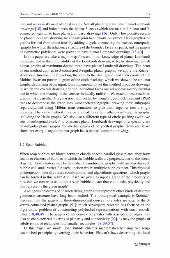
When soap bubbles are blown between closely spaced parallel glass plates, they formfoams or clusters of bubbles in which the bubble walls are perpendicular to the sheets(Fig. 1). These clusters may be described by undirected graphs, with an edge for eachbubble wall and a vertex for each junction where multiple bubbles meet. This physicalphenomenon naturally raises combinatorial and algorithmic questions: which graphscan be formed in this way? And, if we are given as input a graph of the proper type,how can we construct as output a soap bubble cluster that could exist physically andthat represents the given graph?

Analogous problems of characterizing graphs that represent other kinds of discretegeometric structure have long been studied. The prototypical example is Steinitz’stheorem, that the graphs of three-dimensional convex polyhedra are exactly the 3-vertex-connected planar graphs [51]; much subsequent research has focused on thealgorithmic problem of constructing polyhedral representations with small coordi-nates [10,48,49]. The graphs of nonconvex polyhedra with axis-parallel edges mayalso be characterized in terms of planarity and connectivity [22], as may the graphs ofsubdivisions of rectangles into smaller rectangles [38,39,57].

In this paper we model soap bubble clusters mathematically using two long-established principles governing their behavior: Plateau’s laws describing the local

123


Fig. 1 Soap bubbles betweentwo glass plates. Public domainnegative image by Klaus–DieterKeller from Wikimediacommons

geometry of the surfaces and junctions in a bubble cluster, and the Young–Laplaceequation relating the curvature of bubble surfaces to the pressure in each bubble. Wedefine a planar soap bubble cluster to be a family of arcs in the plane that obeys theplanar versions of these principles. It turns out that soap bubbles, defined in this way,are Möbius invariant: Möbius transformation of a planar soap bubble cluster resultsin another physically realizable soap bubble cluster, despite the unphysicality of thistransformation. This fact has been previously used to study planar triple bubbles [60],but as we show it has broader implications. Using Möbius invariance, we provide asimple proof that the graph of every planar soap bubble cluster is 2-vertex-connected,3-regular, and planar. These necessary conditions turn out to be sufficient: every 2-vertex-connected 3-regular planar graph is the graph of a soap bubble cluster. To provethis, we use our Lombardi drawing algorithm: not every Lombardi drawing is a soapbubble cluster, because the drawing may not satisfy the Young–Laplace equation, butthe drawings produced by our algorithm in the 2-vertex-connected case do satisfy thisequation and form valid soap bubbles.

We are not aware of prior attempts to characterize the graphs of soap bubbles,but soap bubbles have been studied mathematically in many other ways. The Kelvinconjecture, stating that a foam with truncated-octahedron cells has the minimum totalsurface area among all soap bubble foams with equal-volume cells, was posed in the19th century by Lord Kelvin and finally solved negatively in 1993 by the discov-ery of the Weaire–Phelan structure, a more parsimonious foam with two differentcell shapes [55,59]; proof that this newer structure is optimal remains elusive. Arelated problem, the minimum-area cap for the ends of hexagonal honeycomb cells,also remains open [27]. It is conjectured that the minimum-surface-area four-bubblecluster, for given bubble volumes, is given by the stereographic projection of a four-dimensional simplex, but this has not been proven, and there are six-bubble clustersfor which the numerically-computed surfaces separating the bubbles are not spheri-

123


cal [53]. Even as simple-sounding a problem as the double bubble conjecture (provingthat the optimal structure for clusters of two bubbles with two fixed volumes has threespherical patches sharing a common circle) took many years to solve [30,34].

Two-dimensional soap films have also seen much prior research, both as a test casefor three-dimensional theories and in the context of the “soap bubble computer”. Inthis device, pegs are placed between two glass plates at specified locations; a soapfilm that connects the pegs forms a minimal (though generally not minimum) Steinernetwork, providing a heuristic and approximate physical solution to an NP-completeproblem [1,6,19,32,35]. Another result on two-dimensional soap films provides aplanar analogue of the Kelvin conjecture: the minimum-length enclosure for an infiniteset of bubbles of equal areas is a hexagonal tiling of the plane [27,28], and similar tilingsarise also as the minimum-length enclosure for finite clusters of equal bubbles [12].

John Sullivan has suggested that “we might look for foams as relaxations of Voronoidecompositions” [53]. Our use of power diagrams to construct bubble clusters may beseen as a validation of Sullivan’s suggestion.

2 Preliminaries

2.1 Möbius Transformations

Let S2 denote the space formed by adding a single point ∞ “at infinity” to the Euclideanplane; this space is also known as the one-dimensional complex projective line P

1(C).In S

2, straight lines may be interpreted as limiting cases of circles, with infinite radiusand containing the point ∞. A Möbius transformation [50] is a map from S

2 to itselfthat transforms every circle (or line) into another circle (or line). Using complex-number coordinates, these transformations may be represented as the fractional lineartransformations

z �→ az + b

cz + d,

and their conjugates. Here a, b, c, and d are complex, and ad − bc �= 0 to prevent thetransformation from defining a constant function. If c = 0 then ∞ is mapped to itself;otherwise, −d/c gets mapped to ∞, and ∞ gets mapped to a/c. Multiplying all fourof a, b, c, and d by the same complex number leaves the transformation unchanged,so the set of Möbius transformations has six real degrees of freedom. This number ofdegrees of freedom is sufficient to allow every triple of distinct points to be mappedby a Möbius transformation to every other triple of distinct points.

Möbius transformations may also be defined from inversions. If O is a circle cen-tered at point o with radius r , inversion through O maps any point p to another point qon the ray from o through p, at distance r2/d(o, p) from o. O is fixed by the inversion,the inside of O becomes the outside and vice versa, and o trades places with ∞. Inthe limiting case of a line, inversion becomes reflection across the line. Every Möbiustransformation may be represented as a composition of a finite set of inversions.

123


Möbius transformations are conformal mappings: they preserve the angle of everytwo incident curves. Since they preserve both circularity and angles, they preserve theproperty of being a Lombardi drawing. Less obviously, we will see later that they alsopreserve the property of being a two-dimensional soap bubble cluster.

2.2 Hyperbolic Geometry

To understand our algorithms, it will be helpful to review some qualitative features ofhyperbolic geometry, avoiding detailed calculations [8].

In the upper halfspace model of three-dimensional hyperbolic space (also calledthe Poincaré halfspace model), hyperbolic space is represented by an open halfspaceof three-dimensional Euclidean space, but with a non-Euclidean distance metric. Theboundary plane of the Euclidean halfspace does not belong to the hyperbolic spacebut may be thought of as the set of “points at infinity” for the hyperbolic space. Itis convenient to add one more point ∞ to this boundary plane, so that it becomes acopy of S

2. Hyperbolic lines are represented by Euclidean semicircles that meet theboundary plane at right angles, or by Euclidean rays perpendicular to the boundaryplane; the vertical rays may be viewed as the limiting case of semicircles with oneendpoint at ∞. Hyperbolic planes are represented by Euclidean hemispheres that meetthe boundary plane at right angles in a circle, or by halfplanes that touch the point ∞and meet the boundary plane perpendicularly in a line.

Hyperbolic space is locally Euclidean: within sufficiently small balls, hyperbolicdistances may be approximated arbitrarily well by Euclidean distances. For every tworeference frames (a choice of a point within the space, and a system of Cartesiancoordinates for the local Euclidean geometry near that point) a unique symmetry ofthe space takes one reference frame into the other. The symmetries of hyperbolic spacemay be extended to the plane at infinity, on which they act as Möbius transformations.Every Möbius transformation of S

2 corresponds uniquely to a symmetry of hyperbolicspace.

2.3 Circle Packing

The Koebe–Andreev–Thurston circle packing theorem [52] states that the vertices ofevery maximal planar graph may be represented by circles with disjoint interiors, suchthat two vertices are adjacent if and only if the corresponding two circles are tangent.The representation is unique up to Möbius transformations. An alternative versionof the theorem, which we use in some of our graph drawing results, states that thevertices of every 3-connected planar graph and of its dual graph may be representedby a combined system of circles in such a way that two circles are tangent if theyrepresent adjacent vertices in the same graph, cross orthogonally if they represent anadjacent vertex-face pair (consisting of one vertex from each graph), and otherwiseare disjoint. Again, this representation is unique up to Möbius transformations [7].

It is not known how to find circle packings in strongly polynomial time, but itis possible to approximate both types of packing by numerical algorithms that arepolynomial in both the number of vertices and the accuracy of approximation [43]. We

123


implemented a numerical relaxation procedure detailed by Collins and Stephenson [11]for finding packings of triangulated planar graphs in which the outer face need not bea triangle and the outer circles have prespecified radii, a more general case than themaximal planar case that we need. Their procedure repeatedly performs the followingsteps:

– It chooses a circle in the packing, and computes the angular defect by which itsneighboring circles either fail to surround it or surround it by a larger angle than2π .

– It determines a representative radius for the neighboring circles such that, if theyall had the representative radius (in place of their actual radii) they would have thesame defect

– It replaces the radius of the central circle by a new value such that, if the surroundingcircles all had the representative radius, the angular defect would be zero.

Each of these steps may be performed using simple trigonometric calculations. AsCollins and Stephenson show, this method converges rapidly to a unique solution, thesystem of radii for a valid packing. Once a close approximation to the radii has beencalculated, the positions of the circle centers are not difficult to determine. Collinsand Stephenson observe that, with small changes, the same procedure can also beused to find orthogonal primal–dual circle packings, or more generally packings withspecified overlap angles between adjacent circles.

The circle packings constructed by the Collins–Stephenson procedure (with equalouter radii) are unsatisfactory for some of our graph drawing applications, because theresulting drawings will have one vertex placed at ∞. To improve our drawings, wefind a Möbius transformation of the packing for which one chosen circle surroundsall the others. Among all transformations fixing the outer circle we choose the onethat maximizes the radius of the smallest inner circle (Fig. 2). This problem of findinga radius-maximizing Möbius transformation may be expressed (using the connectionbetween Möbius transformations and three-dimensional hyperbolic geometry) as aquasiconvex program, a problem of finding the minimum value of a pointwise maxi-mum of quasiconvex functions. It may be solved either combinatorially in linear timeusing LP-type optimization algorithms or numerically using local improvement pro-cedures; the theory of quasiconvex programs guarantees that there are no local optimain which the local improvement might get stuck [4,20]. Since we are already using anumerical method to find circle packings, our implementation also takes the numericalapproach to find the best transformation.

2.4 Triangle Centers

A triangle center is a function from Euclidean triangles to Euclidean points that isequivariant under similarities of the Euclidean plane, in the sense that performinga similarity transformation and then constructing the center gives the same result asconstructing the center and then performing the similarity transformation. Hundredsof triangle centers are known, and they include many well-known points determinedfrom a triangle, such as its centroid, circumcenter, incenter, and orthocenter [37].It is convenient, in computing the position of a triangle center, to use barycentric

123


Fig. 2 Left: the central region of a circle packing constructed by the Collins–Stephenson procedure; theouter three circles, shown only partially in the figure, have equal radii. Right: a transformed packing withone circle exterior to the others, maximizing the minimum circle radius

coordinates, weights for which the center is the weighted average of the vertices.Alternatively, triangle centers may be specified using trilinear coordinates, triples ofnumbers proportional to the distances from each of the triangle’s sides. If the trilinearcoordinates are α : β : γ then the barycentric coordinates are α a : β b : γ c wherethe factors a, b, and c are the lengths of the triangle sides opposite the vertex whoseweight is α, β, or γ respectively.

There are two triangle centers that (as an unordered pair of points) are equivariantunder Möbius transformations, and not just under Euclidean similarities. One of thesetwo centers, the first isodynamic point, may be constructed by transforming the giventriangle to an equilateral triangle (in such a way that the interiors of the circumcirclesof the triangles map to each other), choosing the centroid of the equilateral triangle,and reversing the transformation. The second isodynamic point may be constructedsimilarly using ∞ in place of the centroid. Alternatively, the first isodynamic pointmay be calculated from its trilinear coordinates, which are

sin(A + π/3) : sin(B + π/3) : sin(C + π/3),

where A, B, and C are the three angles of the given triangle. The same formula with−π/3 in place of +π/3 gives the trilinears of the second isodynamic point.

3 Power Diagram

In this section we use three-dimensional hyperbolic geometry to construct, from agiven set D of disks (or complements of disks) in the plane, a diagram M(D) thatpartitions the plane into regions surrounding each disk, separated from each other bycircular arcs. This diagram will be equivariant under Möbius transformations in thesense that, for every Möbius transformation μ, μ(M(D)) = M(μ(D)).

123


3.1 Construction

To construct M(D), let Π be the plane containing D, embed Π into a three-dimensionalEuclidean space, let Π+ be one of the two Euclidean halfspaces having Π as itsboundary, and reinterpret Π+ as a Poincaré halfspace model of three-dimensionalhyperbolic space. Then, the circle bounding each disk Di ∈ D models the set of limitpoints of a hyperbolic plane Pi in this space, and the disk itself is the set of limit pointsof a hyperbolic halfspace Hi . Define the signed distance between a hyperbolic pointq and Hi , for q /∈ Hi , to be the positive distance from q to Pi , and define the signeddistance for q ∈ Hi to be the negation of the distance from q to Pi .

The minimization diagram of this signed distance function is a partition of thehyperbolic space into cells Ci such that, within cell Ci , the signed distance from anypoint of the cell to Hi is smaller than the signed distance to every other halfspaceHj . This diagram is directly defined only for points within the hyperbolic space—thesigned distance is undefined or infinite for points of the boundary plane Π . However,the minimization diagram may be extended to Π by letting the extended cell Ci be thetopological closure of Ci in the halfspace model. We define M(D) to be the restrictionof this extended minimization diagram to the plane Π containing the given disks. Thatis, it is the partition of Π determined by the cells Ci ∩ Π .

3.2 Properties

Lemma 1 For every Möbius transformation μ, μ(M(D)) = M(μ(D)).

Proof Because it is defined using only notions intrinsic to hyperbolic geometry (half-spaces and distance), the minimization diagram from which M(D) is defined is invari-ant under hyperbolic isometries. The result follows from the correspondence betweenhyperbolic isometries and Möbius transformations: each hyperbolic isometry restrictsto a Möbius transformation of the boundary plane of the halfspace model of hyperbolicgeometry, and every Möbius transformation comes from a hyperbolic isometry in thisway. �Lemma 2 The boundaries of the cells in M(D) are circular arcs or subsets of straightlines.

Proof Let Di and D j be any two members of D. First, suppose that Di does not containD j and D j does not contain Di . In this case, we may choose an appropriate Möbiustransformation μ such that μ(Di ) and μ(D j ) are both disks (rather than complementsof disks) with equal radii. By symmetry, M({μ(Di ), μ(D j )}) must have two halfplanecells, separated from each other by the line that perpendicularly bisects the centers ofμ(Di ) and μ(D j ).

Alternatively, suppose that one of the two sets Di and D j contains the other; with-out loss of generality, Di contains D j . In this case, we may choose an appropriateMöbius transformation μ such that μ(Di ) and μ(D j ) are both disks (rather than com-plements of disks) that are concentric. For any point q of hyperbolic space, the signeddistance to Hj will always be smaller than the signed distance to Hi , so in this caseM({μ(Di ), μ(D j )}) consists of a single cell with no boundary.

123


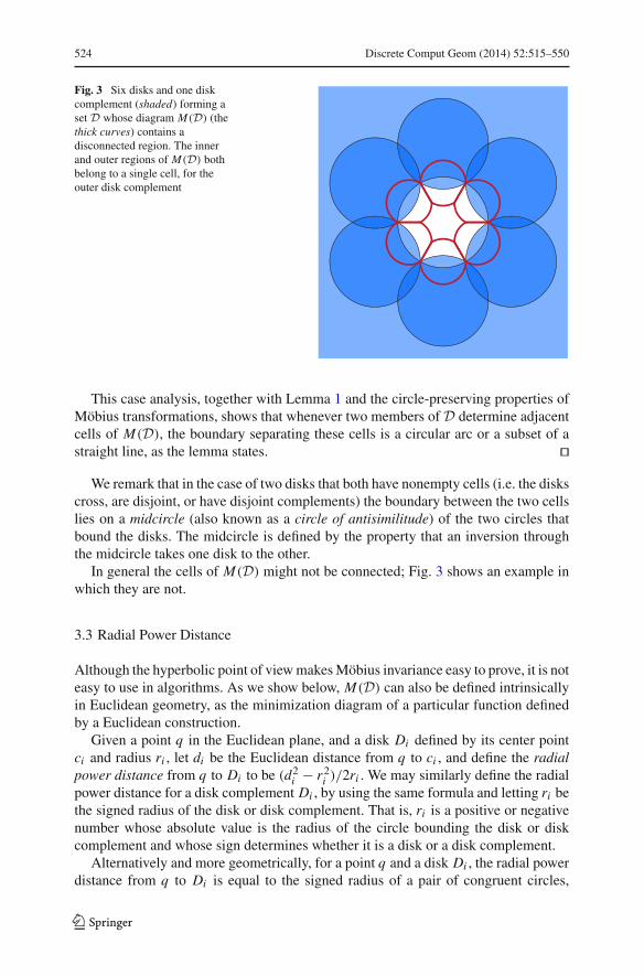
Fig. 3 Six disks and one diskcomplement (shaded) forming aset D whose diagram M(D) (thethick curves) contains adisconnected region. The innerand outer regions of M(D) bothbelong to a single cell, for theouter disk complement

This case analysis, together with Lemma 1 and the circle-preserving properties ofMöbius transformations, shows that whenever two members of D determine adjacentcells of M(D), the boundary separating these cells is a circular arc or a subset of astraight line, as the lemma states. �

We remark that in the case of two disks that both have nonempty cells (i.e. the diskscross, are disjoint, or have disjoint complements) the boundary between the two cellslies on a midcircle (also known as a circle of antisimilitude) of the two circles thatbound the disks. The midcircle is defined by the property that an inversion throughthe midcircle takes one disk to the other.

In general the cells of M(D) might not be connected; Fig. 3 shows an example inwhich they are not.

3.3 Radial Power Distance

Although the hyperbolic point of view makes Möbius invariance easy to prove, it is noteasy to use in algorithms. As we show below, M(D) can also be defined intrinsicallyin Euclidean geometry, as the minimization diagram of a particular function definedby a Euclidean construction.

Given a point q in the Euclidean plane, and a disk Di defined by its center pointci and radius ri , let di be the Euclidean distance from q to ci , and define the radialpower distance from q to Di to be (d2

i − r2i )/2ri . We may similarly define the radial

power distance for a disk complement Di , by using the same formula and letting ri bethe signed radius of the disk or disk complement. That is, ri is a positive or negativenumber whose absolute value is the radius of the circle bounding the disk or diskcomplement and whose sign determines whether it is a disk or a disk complement.

Alternatively and more geometrically, for a point q and a disk Di , the radial powerdistance from q to Di is equal to the signed radius of a pair of congruent circles,

123


Fig. 4 Left: The power distance from the point outside the circle is the length of its tangent segment; thepower distance from the point inside the circle is −1/2 the length of a chord bisected by the point. Right:The radial power distance from the point outside the disk is the radius of the two congruent circles tangentto each other at the point and both tangent to the disk; the radial power distance from the point inside thedisk is the negative radius of the two congruent circles

tangent to each other at q and both tangent to Di (Fig. 4). The sign of this distanceis positive if q is outside D and negative if q is inside D. For a disk complement thedefinition is the same: the radial power distance is equal to the signed radius of a pairof congruent tangent circles, and is positive if q belongs to the disk complement andnegative if it does not. It is straightforward to verify using the Pythagorean theoremthat this geometric definition matches the algebraic one.

We note that this distance function has a similar form to the classical definition ofthe power of a circle, which may be defined algebraically as d2

i − r2i or geometrically

(for points q outside a given disk Di ) as the length of a line segment that has q asone endpoint and whose other endpoint is tangent to Di . The power diagram [3] is theminimization diagram of the power distance, and we claim that our Möbius-invariantpower diagram M(D) coincides with the minimization diagram of the radial powerdistance.

To see the equivalence between the minimization diagrams for three-dimensionalhyperbolic distance and for radial power distance, we use a geometric reformulation ofthe problem of finding nearest neighbors to a query point q. For a point q in hyperbolicspace that is exterior to all of a set of halfspaces, the nearest halfspace may be found(just as in the Euclidean case) as the radius of the smallest sphere centered at q thattouches at least one of the halfspaces, and this sphere is tangent to the halfspace orhalfspaces it touches. Similarly, for a point q that is interior to some of the halfspaces,the minimum signed distance from q to a halfspace is the radius of the largest spherecentered at q that is contained entirely within at least one of the halfspaces, and againthis sphere is tangent to the halfspace or halfspaces that minimize the signed distance.For a point q that is not within the hyperbolic space, but is instead a limit pointof the space, the signed distance from q to the set of halfspaces defined from D isundefined (all curves in hyperbolic space from q to other points have infinite length)but we may still determine the identity of the nearest neighbor of q (that is, the cell ofM(D) containing q) in an analogous way. The geometric figure analogous to a set of

123


Fig. 5 Cross-section of ahalfspace (left) and a horosphereexternally tangent to it (right) inthe halfspace model ofhyperbolic space. The Euclideanplane onto which their shadowsfall is the set of limit points ofthe model, and the black curvesshow the line qc (where q is thepoint at which the horosphere istangent to the plane and c is thecenter of the Euclidean diskfrom which the halfspace wasdefined) and two circles tangentat q whose radius is the radialpower distance

concentric spheres, for a limit point q of the hyperbolic space, is a set of horospheres,sets that appear in the halfspace model of hyperbolic space as spheres tangent at q tothe boundary plane. If q is exterior to all of the given halfspaces, then a hyperbolichalfspace Hi is a nearest neighbor to q if there exists a horosphere centered at q thatis tangent to Hi and disjoint from all of the other halfspaces. If q is contained in someof the halfspaces, then a hyperbolic halfspace Hi is a nearest neighbor to q if thereexists a horosphere centered at q that is tangent to and contained in Hi , and that is notcontained in any of the other halfspaces.

Now let D be any one of the input disks, and consider a planar cross-section ofthe halfspace model of three-dimensional hyperbolic space, defined by a cutting planeperpendicular to the boundary plane of the halfspace model that passes through q andthrough the (Euclidean) center c of D (Fig. 5). Let H be the hyperbolic plane definedfrom disk D; then the intersection of H with the cross-sectional plane is a semicirclecongruent to half of D. The cross-section of the horosphere centered at q and tangentto H is a circle, tangent to this semicircle. If this figure, consisting of a semicircle andtangent circle, is rotated by a right angle around line qc in either of two ways, the tworotated copies of the semicircle together form the boundary circle of D itself, and thetwo rotated copies of the horosphere section form two congruent circles tangent toeach other at q and tangent to this boundary circle; these are the two circles used todefine the radial power distance. Therefore, the nearest neighbor to q in the hyperbolicVoronoi diagram is the disk D for which we can find two congruent circles tangent toeach other at q and tangent to D that are either internally tangent to D and as large aspossible or (if no such disk exists) externally tangent to D and as small as possible.This is the same as the condition defining the nearest neighbor according to radialpower distance, so the two diagrams coincide.

3.4 For Circle Packings

Our applications to graph drawing and soap bubbles use a special case of the diagramM(D) in which the set D of disks and disk complements packs the plane, meaning

123


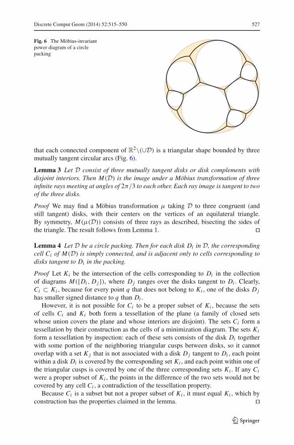
Fig. 6 The Möbius-invariantpower diagram of a circlepacking

that each connected component of R2\(∪D) is a triangular shape bounded by three

mutually tangent circular arcs (Fig. 6).

Lemma 3 Let D consist of three mutually tangent disks or disk complements withdisjoint interiors. Then M(D) is the image under a Möbius transformation of threeinfinite rays meeting at angles of 2π/3 to each other. Each ray image is tangent to twoof the three disks.

Proof We may find a Möbius transformation μ taking D to three congruent (andstill tangent) disks, with their centers on the vertices of an equilateral triangle.By symmetry, M(μ(D)) consists of three rays as described, bisecting the sides ofthe triangle. The result follows from Lemma 1. �

Lemma 4 Let D be a circle packing. Then for each disk Di in D, the correspondingcell Ci of M(D) is simply connected, and is adjacent only to cells corresponding todisks tangent to Di in the packing.

Proof Let Ki be the intersection of the cells corresponding to Di in the collectionof diagrams M({Di , D j }), where D j ranges over the disks tangent to Di . Clearly,Ci ⊂ Ki , because for every point q that does not belong to Ki , one of the disks D j

has smaller signed distance to q than Di .However, it is not possible for Ci to be a proper subset of Ki , because the sets

of cells Ci and Ki both form a tessellation of the plane (a family of closed setswhose union covers the plane and whose interiors are disjoint). The sets Ci form atessellation by their construction as the cells of a minimization diagram. The sets Ki

form a tessellation by inspection: each of these sets consists of the disk Di togetherwith some portion of the neighboring triangular cusps between disks, so it cannotoverlap with a set K j that is not associated with a disk D j tangent to Di , each pointwithin a disk Di is covered by the corresponding set Ki , and each point within one ofthe triangular cusps is covered by one of the three corresponding sets Ki . If any Ci

were a proper subset of Ki , the points in the difference of the two sets would not becovered by any cell Ci , a contradiction of the tessellation property.

Because Ci is a subset but not a proper subset of Ki , it must equal Ki , which byconstruction has the properties claimed in the lemma. �

123


When D is a circle packing, each vertex of the drawing lies within the cusp formedby three mutually tangent circles. By Möbius invariance, this vertex must be placed atthe isodynamic point of the triangle formed by the three points of tangency of this cusp.We may compute its position as the weighted average of the three tangency points,using the known formula for the barycentric coordinates of the isodynamic point tocalculate its weights. Each circular arc of the drawing has two vertices as its end-points and passes through one tangency point, which together determine its location.These facts allow a simple and direct linear-time construction of M(D) (given as inputa combinatorial description of the neighbors to each disk Di of D in clockwise orderaround Di ) using only Euclidean geometry, without any need to perform computationsthat involve hyperbolic coordinates or distances.

4 Lombardi Drawing

In this section we apply our Möbius-invariant power diagram to construct planar Lom-bardi drawings of all subcubic planar graphs, and of some four-regular planar graphs.However, as we show, not every four-regular planar graph has a planar Lombardidrawing.

4.1 Cubic Polyhedral Graphs

We first explain the simplest case of our Lombardi drawing algorithm, in which the pla-nar graph to be drawn is 3-connected and 3-regular. Our drawings may be constructedby the following steps:

– Construct the dual graph of the given input graph, a maximal planar graph, and its(unique) planar embedding.

– Apply the Collins–Stephenson procedure to realize the dual maximal planar graphas the intersection graph of a collection of tangent circles Ci .

– Use quasiconvex programming to find a Möbius transformation of the circlestaking them to a configuration in which one circle C0 is exterior to all the others,and maximizing the minimum radius of the internal circles.

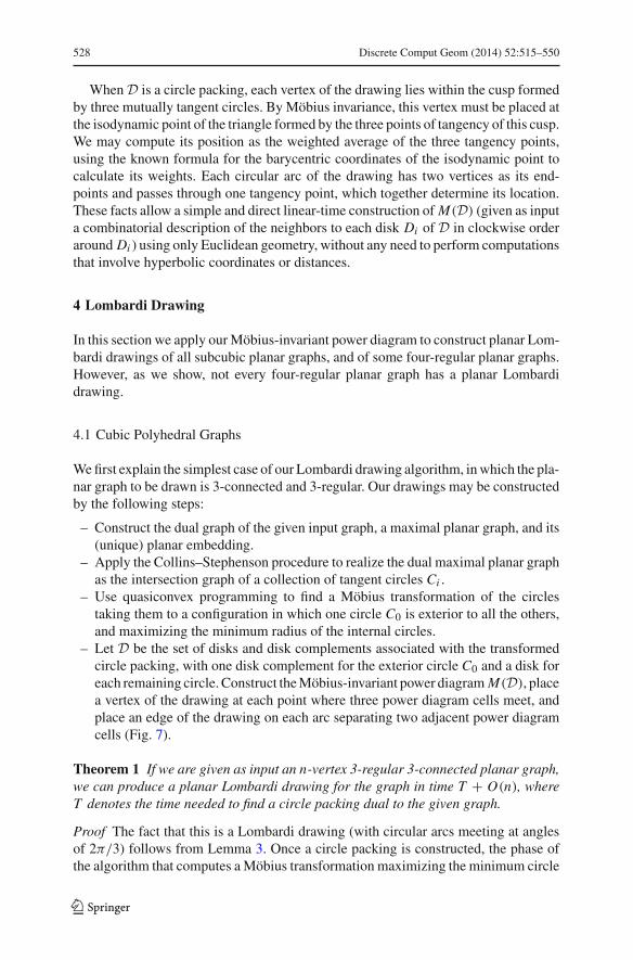
– Let D be the set of disks and disk complements associated with the transformedcircle packing, with one disk complement for the exterior circle C0 and a disk foreach remaining circle. Construct the Möbius-invariant power diagram M(D), placea vertex of the drawing at each point where three power diagram cells meet, andplace an edge of the drawing on each arc separating two adjacent power diagramcells (Fig. 7).

Theorem 1 If we are given as input an n-vertex 3-regular 3-connected planar graph,we can produce a planar Lombardi drawing for the graph in time T + O(n), whereT denotes the time needed to find a circle packing dual to the given graph.

Proof The fact that this is a Lombardi drawing (with circular arcs meeting at anglesof 2π/3) follows from Lemma 3. Once a circle packing is constructed, the phase ofthe algorithm that computes a Möbius transformation maximizing the minimum circle

123


radius can be performed in linear time [4]. The linear time bound for the constructionof M(D) is as described in Sect. 3.4. �

We implemented in Python the algorithm for 3-connected graphs, including theCollins–Stephenson circle packing algorithm and a numerical improvement methodfor finding optimal Möbius transformations. Our implementation takes as input a textfile with one line per vertex; each line lists the identifiers for a vertex and its threeneighbors in clockwise order. The output drawing is represented in the SVG vectorgraphics file format. Figure 8 shows some drawings created by our implementation.

4.2 Two-Connected Subcubic Graphs

We next describe how to extend our Lombardi drawing technique to 2-connectedgraphs. A 2-connected graph may have vertices of degree two or three, but the degree-2vertices may be suppressed, forming a 3-regular multigraph with the same connectivity.If the multigraph has a planar Lombardi drawing, so does the original graph with thedegree-2 vertices, as the vertices may be restored by subdividing edges (placing newvertices in the interior of the circular arc representing the edge) without changing theLombardi property. Therefore, within this section we assume that the given graph is3-regular.

We use a standard tool for decomposing 2-connected graphs, the SPQR tree[13,14,26,33,41]. An SPQR tree for a graph G is a tree structure in which eachtree node is associated with a graph Ci , known as a 3-connected component of G.In each 3-connected component, some of the edges are labeled as “virtual”, and eachedge of the SPQR-tree is labeled by a pair of oriented virtual edges from its two end-points; each virtual edge of a component is associated in this way with exactly onetree edge. The given graph G may be formed by gluing the components Ci together,by identifying pairs of endpoints of virtual edges according to the labeling of the treeedges, and then deleting the virtual edges themselves. The nodes of an SPQR treehave three types: R nodes, in which the associated graph is 3-connected, S nodes, inwhich the associated graph is a cycle, and P nodes, in which the associated graph isa bond graph, a multigraph with two vertices and three or more parallel edges. With

Fig. 7 Lombardi drawing of theFrucht graph [24], one of thetwo smallest 3-regularasymmetric graphs, derivedfrom the circle packing of Fig. 2and the power diagram of Fig. 6

123


(a) (b) (c)

(d) (e) (f)

(g) (h)

Fig. 8 Sample drawings from our implementation. (a) Markström’s 24-vertex graph with no 4- or 8-cycles [42]. (b) Došlic’s 38-vertex graph with girth five and cyclic edge connectivity three [15]. (c) Tutte’s46-vertex non-Hamiltonian cubic planar 3-connected graph [56]. (d) Grinberg’s 46-vertex non-Hamiltoniangraph with cyclic edge connectivity five [25]. (e) 46-vertex Halin graph formed from a complete ternaryfree tree. (f) 252-vertex hexagonal mesh. (g) 60-vertex buckyball or truncated icosahedron. (h) Irregular69-vertex graph

123


S

P

R

R

Fig. 9 Left: The SPQR tree of a planar 3-regular and bridgeless but not 3-connected graph; the dashedblack edges connect pairs of virtual edges to be glued together. Right: A Lombardi drawing formed bytransforming drawings of each 3-connected component so that sets of virtual edges connected to the sameS node all lie on the same circle, removing the arcs of this circle coming from the virtual edges in the P andR nodes, and adding arcs for the real edges of the S node

the additional constraint that no two S nodes and no two P nodes may be adjacent, theSPQR tree is uniquely determined from G, and may be constructed in linear time.

The SPQR trees of 3-regular graphs have an additional structure that will be helpfulfor us:

Lemma 5 (Pootheri [46], Eppstein and Mumford [22]) A 2-connected graph G is3-regular if and only if each edge in its SPQR tree has exactly one S node as anendpoint, each S node is associated with an even cycle that alternates between virtualand non-virtual edges, each P node is associated with a three-edge bond graph, andeach R node is associated with a graph that is itself 3-regular.

Lemma 6 Let G be a graph with a planar Lombardi drawing, and let e be any edgeof G. Then, for any ε > 0 there is a planar Lombardi drawing of G in which e lieson the outer face of the drawing and forms a circular arc that covers an angle of itscircle greater than or equal to 2π(1 − ε).

Proof Transform the given drawing by an inversion whose center is near but not onthe midpoint of e. �

Theorem 2 If we are given as input an n-vertex 2-connected planar graph with max-imum degree 3, we can produce a planar Lombardi drawing for the graph in timeT + O(n), where T denotes the time needed to find and optimally transform a familyof circle packings with total cardinality O(n).

Proof Suppress the degree-two vertices of the given graph to produce a 3-regular2-connected graph, decompose it into an SPQR tree with the additional structureof Lemma 5, and use Theorem 1 to construct a planar Lombardi drawing of the3-connected component associated with each R node. In each S node of the tree, gluethe drawings from the adjacent tree nodes together by using Lemma 6 to expand thevirtual edges, move these edges to the outer face of their drawings, and shrink the restof the drawings, and then align the circular arcs representing their virtual edges so thatthey all lie on a common circle (Fig. 9). Finally, subdivide the edges of the drawingas necessary to restore the suppressed degree-two vertices. �

123


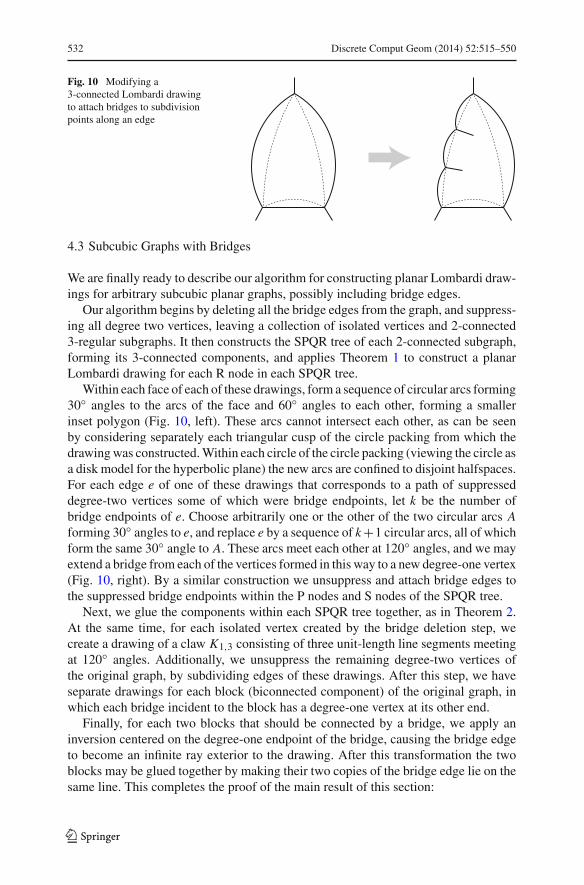
Fig. 10 Modifying a3-connected Lombardi drawingto attach bridges to subdivisionpoints along an edge

4.3 Subcubic Graphs with Bridges

We are finally ready to describe our algorithm for constructing planar Lombardi draw-ings for arbitrary subcubic planar graphs, possibly including bridge edges.

Our algorithm begins by deleting all the bridge edges from the graph, and suppress-ing all degree two vertices, leaving a collection of isolated vertices and 2-connected3-regular subgraphs. It then constructs the SPQR tree of each 2-connected subgraph,forming its 3-connected components, and applies Theorem 1 to construct a planarLombardi drawing for each R node in each SPQR tree.

Within each face of each of these drawings, form a sequence of circular arcs forming30◦ angles to the arcs of the face and 60◦ angles to each other, forming a smallerinset polygon (Fig. 10, left). These arcs cannot intersect each other, as can be seenby considering separately each triangular cusp of the circle packing from which thedrawing was constructed. Within each circle of the circle packing (viewing the circle asa disk model for the hyperbolic plane) the new arcs are confined to disjoint halfspaces.For each edge e of one of these drawings that corresponds to a path of suppresseddegree-two vertices some of which were bridge endpoints, let k be the number ofbridge endpoints of e. Choose arbitrarily one or the other of the two circular arcs Aforming 30◦ angles to e, and replace e by a sequence of k +1 circular arcs, all of whichform the same 30◦ angle to A. These arcs meet each other at 120◦ angles, and we mayextend a bridge from each of the vertices formed in this way to a new degree-one vertex(Fig. 10, right). By a similar construction we unsuppress and attach bridge edges tothe suppressed bridge endpoints within the P nodes and S nodes of the SPQR tree.

Next, we glue the components within each SPQR tree together, as in Theorem 2.At the same time, for each isolated vertex created by the bridge deletion step, wecreate a drawing of a claw K1,3 consisting of three unit-length line segments meetingat 120◦ angles. Additionally, we unsuppress the remaining degree-two vertices ofthe original graph, by subdividing edges of these drawings. After this step, we haveseparate drawings for each block (biconnected component) of the original graph, inwhich each bridge incident to the block has a degree-one vertex at its other end.

Finally, for each two blocks that should be connected by a bridge, we apply aninversion centered on the degree-one endpoint of the bridge, causing the bridge edgeto become an infinite ray exterior to the drawing. After this transformation the twoblocks may be glued together by making their two copies of the bridge edge lie on thesame line. This completes the proof of the main result of this section:

123


Theorem 3 If we are given as input an n-vertex planar graph with maximum degree 3,we can produce a planar Lombardi drawing for the graph in time T + O(n), whereT denotes the time needed to find and optimally transform a family of circle packingswith total cardinality O(n).

4.4 Halin Graphs

The method of constructing Lombardi drawings from a packing of disjoint tangentcircles, used above for 3-regular polyhedral graphs, applies to some other graphsas well. We define a system of interior-disjoint disks D to be well-centered if theMöbius-invariant power diagram M(D) forms a system of arcs and vertices that formsa Lombardi drawing of the planar dual to the intersection graph of D. Equivalently, Dis well-centered when its diagram has one vertex within each connected componentof the complement R

2\D of D, and when all cell boundaries incident to that vertexmeet at equal angles. If a planar graph G has a dual graph that can be represented bya well-centered system of disks D, then M(D) will form a Lombardi drawing of G.

As an example of a system of disks that is not a disk packing but is well-centered,consider k congruent disks with centers all on a common circle, sized so that each diskis tangent to its two neighbors on the circle. In this case, the intersection graph of Dis a k-cycle, and M(D) is a system of k rays meeting at equal angles. By performingan appropriate Möbius transformation of D, we may perturb it so that M(D) forms asystem of k circular arcs, meeting at equal angles at two points, one of which is thetransformation of the center of the circle and the other of which is the transformationof ∞. This is a Lombardi drawing of a multigraph with k edges and two vertices, theplanar dual of the k-cycle.

As a less trivial example, let G be any Halin graph [29], a 3-connected planar graphformed from a plane tree (with no degree-two vertices) by adding a cycle connecting itsleaves in the order given by the plane embedding of the tree. As a polyhedral graph, Gcan be represented (uniquely up to Möbius transformation) by a pair of circle packingsD and D′, where the intersection graph of D is the dual graph of G, the intersectiongraph of D′ is G itself, and adjacent pairs of vertices in G and its dual (correspondingto an incident vertex-face pair in G) are represented by orthogonal circles in D andD′. We claim that D is well-centered. For, if v is a vertex on the outer face of G, ithas degree three and is surrounded by three mutually tangent disks, for which well-centeredness follows from Lemma 3. Alternatively, if v is an interior vertex of G, thenthe k circles surrounding v (where k is the degree of v in G) are all orthogonal tothe circle representing v and tangent to the circle representing the outer face of G. Itfollows that the set of circles surrounding v is Möbius-equivalent to the system of kconcyclic circles described above for the k-cycle, and so is well-centered. Therefore,M(D) is a Lombardi drawing of G.

It was previously known that every Halin graph had a planar Lombardi draw-ing [18] but the previous construction involved certain arbitrary choices. In contrast,this method, based as it is on the unique orthogonal circle packing for 3-connectedplanar graphs and their duals, provides a principled and unique way of making thosechoices for every Halin graph.

123


Fig. 11 Dual circle packingsfor a cube and octahedron, witha Lombardi drawing of theirmedial graph, the cuboctahedron

4.5 Four-Regular Medial Graphs

A variant of the circle packing theorem states that every 3-connected planar graphG and its dual can be simultaneously represented by tangent circles, so that twocircles from the two packings are orthogonal if they represent a vertex v of G and aface of G containing v, and disjoint otherwise. The packing is unique up to Möbiustransformation, and may be found by a numerical procedure similar to the one for circlepacking of maximal planar graphs [43]. These dual packings allow us to construct aplanar Lombardi drawing of the medial graph of G, the 4-regular graph formed byplacing a vertex on the midpoint of each edge of G and connecting two of these newvertices by an edge whenever they are the midpoints of consecutive edges on the sameface. Each pair of orthogonal circles in the packing and dual packing of G form alune, which may be bisected by a circular arc forming a π/4 angle with both circles.When two of these bisecting circular arcs meet at the same point of tangency of thecircle packing, they form an angle of π/2 or π to each other. Therefore, we have aLombardi drawing of the four-regular graph that has a vertex at each tangency pointof the packing and an edge for each of these bisecting arcs. This graph is the medialgraph of G (Fig. 11). As was the case for 3-regular polyhedral graphs, this drawinghas an interpretation as the Möbius-invariant power diagram M(D) of a collection ofdisks D that includes a disk for each circle in the circle packing for G and its dual.

As with our technique for finding Lombardi drawings of subcubic graphs, thedrawings constructed in this way can be extended to certain 2-connected graphs usingthe SPQR tree. However, this technique does not apply to 3-connected 4-regular planargraphs that are not medial graphs of polyhedral graphs, such as the one shown in Fig. 12.More strongly, in the next section we show that there exist 4-regular planar graphs thathave no planar Lombardi drawing.

4.6 A 4-Regular Graph with No Planar Lombardi Drawing

The 4-regular 2-connected planar graph G18 in Fig. 13 has no planar Lombardi draw-ing, as we now prove.

123


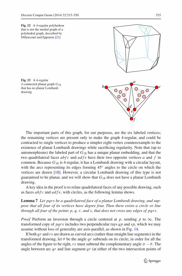
Fig. 12 A 4-regular polyhedronthat is not the medial graph of apolyhedral graph, described byDillencourt and Eppstein [21]

Fig. 13 A 4-regular2-connected planar graph G18that has no planar Lombardidrawing

ab c

de

f

The important parts of this graph, for our purposes, are the six labeled vertices;the remaining vertices are present only to make the graph 4-regular, and could becontracted to single vertices to produce a simpler eight-vertex counterexample to theexistence of planar Lombardi drawings while sacrificing regularity. Note that (up toautomorphisms) the labeled part of G18 has a unique planar embedding, and that thetwo quadrilateral faces ab f c and ad f e have their two opposite vertices a and f incommon. Because G18 is 4-regular, it has a Lombardi drawing with a circular layout,with the arcs representing its edges forming 45◦ angles to the circle on which thevertices are drawn [18]. However, a circular Lombardi drawing of this type is notguaranteed to be planar, and we will show that G18 does not have a planar Lombardidrawing.

A key idea in the proof is to relate quadrilateral faces of any possible drawing, suchas faces ab f c and ad f e, with circles, as the following lemma shows.

Lemma 7 Let pqrs be a quadrilateral face of a planar Lombardi drawing, and sup-pose that all four of its vertices have degree four. Then there exists a circle or linethrough all four of the points p, q, r , and s, that does not cross any edges of pqrs.

Proof Perform an inversion through a circle centered at p, sending p to ∞. Thetransformed copy of pqrs includes two perpendicular rays qp and sp, which we mayassume without loss of generality are axis-parallel, as shown in Fig. 14.

If both qr and rs are drawn as curved arcs (rather than straight line segments) in thetransformed drawing, let θ be the angle qr subtends on its circle; in order for all theangles of the figure to be right, rs must subtend the complementary angle π − θ . Theangle between arc qr and line segment qr (at either of the two intersection points of

123


Fig. 14 Figure for proof ofLemma 7 p

p

O

s

q

r

θπ – θ

these two curves) is θ/2, and symmetrically the angle between arc rs and line segmentrs is (π − θ)/2. Angle qrs is equal to the sum of these two angles together with theright angle between the two arcs; that is, it is θ/2 + π/2 + (π − θ)/2 = π . Thus,q, r , and s are collinear.

If one of qr and rs (say qr ) is not a curved arc, but a straight line segment, it mustbe axis-parallel in order to form a right angle at q, and the other arc rs must be asemicircle in order to form right angles at r and s. Again, in this case, q, r , and s arecollinear.

In either case, the line O through the three points q, r , and s also passes throughp = ∞ (because every line passes through ∞). Reversing the inversion we initiallyperformed, O becomes the desired circle. It can’t cross the circular arcs of pqrsbecause two circles can only intersect at two points and each of these arcs alreadyintersects O at its two endpoints. �

Theorem 4 Graph G18 has no planar Lombardi drawing.

Proof If G18 had a planar Lombardi drawing, then by Lemma 7 its quadrilateral facesad f e and ab f c would have circumscribing circles. If they do not coincide, thesecircles intersect at the two vertices a and f ; the other four vertices must be placedbetween them on the four circular arcs connecting these two intersection points. Byperforming an inversion centered within face ab f c we may assume without loss ofgenerality that the drawing resembles the schematic layout shown in Fig. 15, in thesense that face ab f c lies outside of its circle. The other circle, ad f e, must contain onebut not both of the vertices b and c; without loss of generality we assume it contains cand does not contain b, because the other case is symmetric under a relabeling of thevertices. Then (in order for the drawing to be planar) vertex d may be placed anywherealong the arc of circle ad f e closest to b. The ray from c radially outwards from thecenter of circle ab f c lies entirely within face ab f c, and crosses circle ad f e; vertex emay be placed on its arc either above or below this ray, but by symmetry (flipping thediagram and relabeling the vertices if necessary) we assume that it is above the ray, asdepicted schematically in the figure.

123


Fig. 15 Figure for proof ofTheorem 4 a

b

c

d

e

f

?

For this placement, the edge ce must exit vertex c towards the interior of circleab f c, because it forms a 180◦ angle with either edge ac or edge f c, both of whichare exterior to the circle. It must then cross circle ab f c again, turning clockwise as itdoes, in order to stay within quadrilateral ae f c and reach vertex e. By a symmetricargument it must exit vertex e towards the exterior of circle ad f e, because it formsa 180◦ angle with either edge ae or edge f e, both of which are interior to the circle.Thus, coming from c, it must cross circle ad f e, turning counterclockwise as it does, toreach the circle a second time. But in a Lombardi drawing, edge ce must be drawn asa circular arc, which cannot turn clockwise for part of its length and counterclockwisefor part of its length. Therefore, this placement is impossible.

The remaining case arises when circles ab f c and ad f e coincide. But in this case,by similar reasoning, edge ce must exit c towards the interior of the single circle, crossthe circle, and reach e from the exterior, an impossibility since a circular arc cannothave three intersection points with a circle. �

5 Soap Bubbles

As we show in this section, our Möbius-invariant power diagram can be used toconstruct planar soap bubble clusters with any realizable topology, leading to a graph-theoretic characterization of these clusters.

5.1 A Mathematical Model of Soap Bubbles

Two classical results describe the geometry of soap bubbles. Plateau’s laws, observedexperimentally in the 19th century by Joseph Plateau [45] and proven rigorously forminimal surfaces in 1976 by Jean Taylor [54], state that in a three-dimensional soapbubble cluster,

– Each two-dimensional surface has constant mean curvature. That is, the two prin-cipal curvatures of the surface take the same average value at all points in thesurface.

123


– At each one-dimensional junction of surfaces, exactly three surfaces meet, andthey form dihedral angles of 2π/3 with each other. Such a junction is called aPlateau border. A Plateau border may either be a simple closed space curve or acurve with two endpoints, in either case touching the same three surfaces for itsentire length.

– At each endpoint of a Plateau border, exactly four Plateau borders and six two-dimensional surfaces meet, and the borders form angles of cos−1(−1/3) with eachother (the same angle that is formed by rays from the center of a regular tetrahedronthrough its vertices).

The Young–Laplace equation, also formulated in the 19th century by Thomas Youngand Pierre-Simon Laplace, states that the mean curvature of a two-dimensional surfacein a soap bubble cluster is proportional to the difference in pressure on the two sidesof the surface, with a constant of proportionality determined by the surface tension ofthe fluid forming the soap bubbles [36].

In the case of a soap bubble cluster formed between two flat plates, the bubble wallsare perpendicular to the plates, and all cross-sections of the bubbles by a plane parallelto one of the plates are congruent to each other. In this case, the principal curvaturein the direction perpendicular to the plates is zero, and we may simplify both laws todescribe the planar figure formed by the cross-sections.

Thus, the two-dimensional restriction of Plateau’s laws state that:

– The figure consists of one-dimensional curves of constant curvature; that is, circulararcs or line segments that do not cross each other.

– At each endpoint of one of these arcs or segments, exactly three curves meet, andthey form angles of 2π/3 with each other.

Correspondingly, the two-dimensional restriction of the Young–Laplace equationstates that:

– The curvature of any one of the circular arcs (the inverse of its radius) is pro-portional to the difference in pressure between the bubbles it separates. Bubbleswith the same pressure as each other are separated by line segments, with zerocurvature.

We define a planar soap bubble cluster to be a finite collection of curves, obeyingthe planar restrictions of Plateau’s laws and the Young–Laplace equation (for someassignment of pressures to each bubble). Equivalently, in graph-theoretic terminology,it is a planar embedding of a graph with circular-arc edges, forming angles of 2π/3at each vertex, for which it is possible to find a pressure assignment to the bubblesthat is consistent with all of the arc curvatures. As we describe in Sect. 5.2, we canreplace this existential condition (the existence of a consistent pressure assignment)with a simpler statement about the curvatures of triples of arcs meeting at vertices. Ina planar soap bubble cluster, the local forces on each vertex or arc caused by pressureand surface tension will sum to zero, so it will be in an equilibrium (though possiblyan unstable one [23,58]).

As our results will later show, the Lombardi drawings depicted in Figs. 6 and 8(minus the vertex disks) form examples of soap bubble clusters. In contrast, Fig. 16depicts a planar 3-regular Lombardi drawing that is not a soap bubble cluster, because

123


Fig. 16 A collection ofsegments and arcs that obeysPlateau’s laws, but does not forma planar soap bubble cluster,because it has no valid pressureassignment consistent with itsarc curvatures. Three of itssegments do not separatedifferent regions, impossible forsoap bubbles

it disobeys the Young–Laplace equation. There is no assignment of pressures to thebubbles in this figure that is consistent with the curvatures of its arcs, and at the sixasymmetric vertices in the figure, the curvatures of the three incident arcs do not sumto zero, violating the local reformulation of the Young–Laplace equation described inSect. 5.2.

5.2 Localization of the Young–Laplace Equation

It is convenient to replace the Young–Laplace equation with a more local criterion,using a signed variation of curvature. Given a circular arc ending at a point p, ofcurvature c ≥ 0, we define the signed curvature of the arc at p to be c whenever thearc curves clockwise as it leaves p, and to be −c whenever it curves counterclockwise.For line segments, of course, the signed curvature is zero.

Lemma 8 A finite collection of circular arcs and line segments forms a planar soapbubble cluster if and only if it obeys Plateau’s laws and, at each endpoint of an arc orsegment, the sum of the signed curvatures of the three incoming curves is zero.

Proof In one direction, in a planar soap bubble cluster, let x , y, and z be the pressuresof three bubbles that meet at a point. By assumption, the cluster obeys the Young–Laplace equation, according to which the three signed curvatures of the arcs at thepoint are proportional to the pressure differences x − y, y − z, and z − x . The factthat these three signed curvatures sum to zero follows from the simple algebraic factthat (x − y) + (y − z) + (z − x) = 0.

In the other direction, suppose that finitely many circular arcs obey Plateau’s lawsand have signed curvatures adding to zero at each point where three arcs meet. Wemust assign pressures to the bubbles formed by the arcs, such that the curvatures obeythe Young–Laplace equation. Assign zero pressure to the outside region. For eachbounded bubble B, choose arbitrarily a curve c that starts in the outside region, endswithin B, meets the arcs only at proper crossing points interior to an arc, and hasfinitely many crossing points. Set the pressure within B to the sum of the pressuredifferences determined by the curvatures of each crossed arc.

123


To show that this system of pressures obeys the Young–Laplace equation, considerany two bubbles B1 and B2 separated by an arc A, and let c1 and c2 be the curvesfrom the outside region to B1 and B2 by which their pressures were determined. Wemay link c1 and c2 by another curve that remains entirely within the outside region,forming a single (possibly self-crossing) curve that connects B1 to B2, and we maycontinuously deform this curve, crossing finitely many triple points of the system ofarcs as we do, until it forms a line segment crossing arc A. Each time this deformationcauses the curve to cross a triple point, the assumption that the curvatures at that pointadd to zero ensures that the sum of the pressure differences of crossings along thecurve remains constant. Before the deformation, this sum was the pressure differencebetween B1 and B2 in our system of pressures, and after the deformation, it is thepressure difference required between bubbles B1 and B2 for the curvature of A toobey the Young–Laplace equation. Since these two pressure differences are equal, A(and by the same argument every arc) obeys the equation. �

An analogous result for bubbles on the sphere instead of the plane is in QuinnMaurmann’s appendix to [47].

When three three-dimensional bubbles form a cluster in which all surface patchesare spherical, it was known to Plateau that the three inner surface patches have cen-ters of curvature that all lie on a single line [31]. Although centers of circles andcollinearity of points are not Möbius-invariant properties, we can restate the samecollinearity property for planar bubble clusters in a Möbius-invariant way, in termsof the crossing points of the circles. This restatement will allow us to prove that theMöbius transformation of a planar soap bubble cluster is itself another planar soapbubble cluster.

Lemma 9 Let three circular arcs meet at angles of 2π/3 at a point X, with centersof curvature Ci for i ∈ {1, 2, 3}, and let ri = |XCi | be the radii of each of the threearcs. Then the following three conditions are equivalent:

1. The sum of the three signed curvatures of the arcs is zero.2. The three center points Ci are collinear.3. The three circles with centers Ci and radii ri have two triple crossing points.

Proof We partition the proof into four implications between the three conditions ofthe lemma.

(1) ⇒ (2): Suppose that the three signed curvatures sum to zero; then one musthave a different sign than the other two. Without loss of generality (by permutingthe indices and by mirroring the configuration, if necessary) we may assume that thesigned curvatures are 1/r1, −1/r2, and 1/r3. By assumption, the sum of these threequantities is zero; by multiplying each term of this sum by r1r2r3 and rearranging, weobtain the equation r1r2 + r2r3 = r1r3.

Note that the three lines XCi form angles of π/3 with each other, because they areperpendicular to the arcs, which meet at angles of 2π/3. The assumption on the signsof the curvatures implies that angles C1 XC2 and C2 XC3 must both equal π/3, andangle C1 XC3 must equal 2π/3. Now consider the areas of the three triangles C1 XC2,C2 XC3, and C1 XC3. In any triangle, the area can be computed by the side-angle-side

123


X

C1C2 C3

Fig. 17 Arcs meeting the conditions of Lemma 9

formula as half the product of two adjacent side lengths with the sine of the angleformed by the same two sides. Thus, these triangle areas are 1

2r1r2 sin π3 , 1

2r2r3 sin π3 ,

and 12r1r3 sin 2π

3 respectively. But sin π/3 = sin 2π/3, so the already-obtained equa-tion r1r2 + r2r3 = r1r3 implies that triangles C1 XC2 and C2 XC3 together have thesame total area as triangle C1 XC3. This could only happen if the three centers C1,C2, and C3 are collinear, for otherwise the sum of the areas of C1 XC2 and C2 XC3would differ from the area of C1 XC3 by the area of triangle C1C2C3, which is zeroonly when these three points are collinear.

(2) ⇒ (1): By (2) the three center points Ci are collinear; assume without loss ofgenerality that C2 lies between C1 and C3 on their common line. Because the threecenters C1, C2, and C3 form angles of π/3 rather than 2π/3, the signed curvatureof the middle center C2 has the opposite sign to the signed curvature of the otherthree curvatures; we may assume without loss of generality (by mirror reversing theconfiguration if necessary) that these three signed curvatures are 1/r1, −1/r2, and1/r3. As in the previous case, the three lines XCi form angles of π/3 with each otherso angles C1 XC2 and C2 XC3 must both equal π/3, angle C1 XC3 must equal 2π/3,and by collinearity the two triangles C1 XC2 and C2 XC3 together disjointly cover thesame region of the plane as the single triangle C1 XC3.

We can apply the side-angle-side formula to this region in two different ways, givingthe equation

1

2r1r2 sin

π

3+ 1

2r2r3 sin

π

3= 1

2r1r3 sin

2π

3.

But the factors of 1/2 cancel, as do the factors of sin π/3 = sin 2π/3, leaving thesimpler equation r1r2 +r2r3 = r1r3. Dividing all terms by r1r2r3 gives 1/r3 +1/r1 =1/r2, and rearranging gives 1/r1 − 1/r2 + 1/r3 = 0 as desired.

123


(2) ⇒ (3): The three circles have at least one triple crossing point, at X . Let be theline through the three centers, assumed to exist by (2). Then because passes througheach circle center, a reflection across is a symmetry of each circle and therefore ofthe whole configuration of three circles. The point X cannot lie on , because twocircles centered on a line cannot cross at a point that is also on the line, they can onlymeet at a point of tangency, violating the assumption that the arcs meet at angles of2π/3. Therefore, the reflection of X across is also a triple crossing point, and thethree circles have two triple crossings as (3) states.

(3)⇒ (2): For any two intersecting circles, it is necessarily true that their centers lieon the perpendicular bisector of the chord connecting their two intersection points. Butby the assumption of (3) that there are two triple crossing points, the chords defined byeach pair of the three given circles coincide; therefore, their perpendicular bisectorsalso coincide in a line that contains all three circle centers. �

Figure 17 shows a set of arcs, circles, centers, and radii meeting the conditions ofthe lemma. The lemma applies directly only to circular arcs and not to straight linesegments; for line segments we need a more careful statement.

Lemma 10 Let three circular arcs or straight line segments meet at angles of 2π/3at a point X. Then the following two conditions are equivalent:

1. The sum of the three signed curvatures of the arcs and segments is zero.2. The three circles or lines containing the three arcs or line segments have two triple

crossing points (possibly including the point at infinity).

Proof We consider different cases for each possible number of straight line segmentsin the input configuration.

– When there are no segments and three circular arcs, the lemma is just a simplifiedformulation of Lemma 9.

– When there is one line segment and two circular arcs, the curvature sum is zeroif and only if the two arcs are reflections of each other across the line segment(otherwise their two curvatures cannot cancel) and there is a second triple crossingpoint if and only if the same reflection condition is met (otherwise the two circleswill cross the line in different points).

– When there are two line segments and one circular arc, the sum of the curvaturesis always nonzero (it equals the curvature of the circular arc), and there is only onetriple crossing point (the two lines have their second intersection at infinity andtheir intersections with the circle at finite points).

– When there are three line segments, the sum of the curvatures is always zero, asall curvatures are themselves zero, and the three lines meet at X and at the pointat infinity, so both conditions are true.

Since the equivalence holds in each possible case, it holds in general. �This triple crossing property is closely related to Lemma 5.1 of [60] and to the

existence and uniqueness of the standard double bubble, for which see e.g. Proposition14.1 of [44].

123


5.3 Möbius Invariance

Möbius transformations do not preserve physically meaningful quantities of soapbubbles such as their pressures or the total length or area of soap film. They do noteven preserve the finiteness of the bubbles: it is possible to find a transformationthat takes the unbounded region of the plane to a bounded region and vice versa.Nevertheless, surprisingly, they transform soap bubble clusters into other soap bubbleclusters. We outline a proof of Möbius invariance below.

Lemma 11 Let B be a planar soap bubble cluster, and let μ be a Möbius transfor-mation with the property that no curve or arc of B is transformed into a ray or doubleray. Then μ(B) is also a planar soap bubble cluster.

Proof By Lemmas 8 and 10, B consists of arcs or segments meeting at angles of 2π/3such that each three arcs that meet have circles forming two triple crossings. The meet-ing angles and the triple crossings of circles are preserved by Möbius transformation,so μ(B) is also a collection of arcs or segments meeting at angles of 2π/3 such thateach three arcs that meet have circles forming two triple crossings. By Lemma 10 again,the signed curvatures at each meeting point of μ(B) add to zero, and by Lemma 8again, μ(B) is a planar soap bubble cluster. �

5.4 Bridgelessness

Based on the Möbius invariance of planar soap bubble clusters, we prove in this sectionthe necessity of our graph-theoretic characterization: every planar soap bubble clustercomes from a graph that is planar, 3-regular, and 2-connected.

It is clear that a planar soap bubble cluster must form a planar graph, and Plateau’slaws imply that it must be 3-regular, so the nontrivial part of our characterization of soapbubble graphs is the claim that these graphs are 2-vertex-connected, or equivalently(since they are three-regular) that they have no bridges. In the language of soap bubbles,this means that every arc or segment in the cluster separates two different bubbles. Aswe now prove, this is necessarily true for a planar soap bubble cluster.

Lemma 12 In a planar soap bubble cluster, no segment or arc can have the samebubble on both of its sides.

Proof Assume for a contradiction that the cluster includes a segment or arc e that hasthe same bubble on both sides. Nonzero curvature of e would contradict the Young–Laplace equation, as the pressure is equal on both sides of e. But if e is a line segment,then it is straightforward to find a Möbius transformation that transforms e into acurved arc. The resulting cluster again contradicts the Young–Laplace equation, andby Lemma 11, the untransformed cluster also contradicts the same equation. �

5.5 Realizing Graphs as Soap Bubbles

As we now show, the steps of our Lombardi drawing algorithm that apply to 2-connected or 3-connected graphs generate soap bubble clusters, giving us an algo-

123


rithmic proof that our necessary conditions for a graph to be the graph of a soapbubble cluster are also sufficient.

Lemma 13 Let D be a set of three mutually tangent circles. Then their Möbius-invariant power diagram M(D) is a double bubble formed by three circular arcs, linesegments, or rays, meeting in two triple crossing points at angles of 2π/3, with signedcurvatures summing to zero.

Proof By Lemma 3, M(D) is the image under a Möbius transformation of three raysmeeting at angles of 2π/3. These rays meet in two triple crossing points, the commonapex of the rays and the point at infinity, and this triple crossing property is preservedunder Möbius transformation. The claim that the curvatures of the transformed rayssum to zero follows from Lemma 10. �Theorem 5 A multigraph G can be realized as the arcs and junctions of a planarsoap bubble cluster if and only if G is planar, 3-regular, and bridgeless.

Proof Planarity and 3-regularity follow from Plateau’s laws. The requirement that aplanar soap bubble cluster be bridgeless is Lemma 12. It remains to show that everyplanar, 3-regular, and bridgeless graph G may be realized as a soap bubble.

If G is planar, 3-regular, and 3-connected, then (as in Sect. 4.1) G may be drawnas the Möbius-invariant power diagram M(D) for a circle packing D representing thedual graph of G. At each vertex of the diagram, the regions for three mutually tangentcircles of D meet. By Lemma 13, the vertex is incident to three circular arcs meetingat angles of 2π/3 (satisfying Plateau’s laws), with signed curvatures summing to zero.Therefore, by Lemma 8, the diagram forms a planar soap bubble cluster representing G.

Finally, if G is bridgeless, planar, and 3-regular but not 3-connected, it must be2-connected. In this case, as in Sect. 4.2 and Fig. 9, it may be formed by constructingan SPQR tree representing the 3-connected components of G, separately drawing each3-connected component as a double bubble or as the Möbius-invariant power diagramof a circle packing, transforming these drawings so that they do not cross each otherand so that the virtual edges that connect to each S node lie on a common circle,deleting the virtual edges, and drawing the real edges of the S node along the sharedcircle. As in the 3-connected case, the drawing of each component obeys Plateau’slaws and has zero curvature sum at each vertex. By Lemma 11, these properties arepreserved by the step of the drawing algorithm that transforms each component. Thestep of the algorithm that deletes the virtual edges and replaces them by real edgesdoes not change the local geometry at any vertex of the drawing, so again it preservesthe properties of obedience to Plateau’s laws and zero local curvature sum. Thus, afterthese steps we have a drawing that continues to obey these properties. By Lemma 8,the diagram forms a planar soap bubble cluster representing G. �

We note that, although our circle packing method is capable of realizing all graphsof planar soap bubble clusters, it is not capable of generating all valid geometries ofplanar soap bubble clusters. In particular, in the 3-connected case, the clusters wegenerate have the property that within each bubble there is a circle tangent to all thearcs of the bubble, but this property does not hold for arbitrary soap bubble clusters.For instance, not all of the bubbles in Fig. 1 have this property.

123


5.6 Stability

So far, we have been considering only whether a bubble cluster is in equilibrium ornot, but we may differentiate what kind of equilibrium a cluster is in by its stability,describing the relation between the energy of the equilibrium to the energy of nearbyconfigurations. To do this, we need some additional definitions. In the case of bubbleclusters, we may define a configuration to be a family of locally-smooth curves thatpartitions space into a fixed number of regions (where each region may not necessarilybe connected). A neighborhood of a given configuration B is the set of all configura-tions for which the Hausdorff distance of each region to the corresponding region ofB is within some threshold.

There are two natural ways of defining the energy of a configuration. If each bubblein the cluster contains a fixed quantity of a compressible gas, then the energy maynaturally be defined as the sum of two terms, one for the tension of the bubble walls andthe other for the pressure within the bubbles. That is, the energy is γ L+∑

Pi Ai , whereAi is the area of the i th bubble, Pi is the difference of its pressure (modeled accordingto the ideal gas law) from ambient, L is the total length of the curves in the cluster, andγ is the surface tension, the constant of proportionality of the Young–Laplace equation.Alternatively, we may restrict the neighborhood of a configuration to maintain a fixedarea for each bubble, and use only the first term γ L for the energy; this describes alimiting case in which each bubble contains a fixed quantity of incompressible liquid.

With these definitions for neighborhoods and energy, a stable equilibrium is abubble cluster that uniquely attains the minimum energy. A metastable equilibrium isa bubble cluster that is not stable, but that has a neighborhood within which it uniquelyattains the minimum energy. An unstable equilibrium is a bubble cluster for whichall neighborhoods contain a cluster with lower energy. And a neutral equilibrium is abubble cluster that is neither metastable nor unstable: every neighborhood contains adifferent cluster with equal or lower energy, but there exists a neighborhood that doesnot contain any lower-energy state.

When all four kinds of equilibrium are allowed, Theorem 5 characterizes the graphsof equilibrium bubble clusters. However, disallowing unstable and neutral equilibriachanges this characterization, as we now show. To do so, we use Möbius invarianceagain, to prove that non-3-connected clusters necessarily include cocircular featuresthat are incompatible with stability.

Lemma 14 Let G be the graph of a planar soap bubble cluster B, having two edgese1 and e2 such that G\{e1, e2} is disconnected. Then in B, e1 and e2 form cocirculararcs or collinear segments.

Proof Suppose for a contradiction that e1 and e2 lie on distinct circles or lines. Then, wecould find a point q that lies on the circle or line containing e1 (but does not belong to e1itself), is disjoint from the circle or line containing e2, and is also disjoint from all otherarcs of B. By Lemma 11, a Möbius transformation μ defined by inversion throughq would transform B into another bubble cluster μ(B), in which μ(e1) becomes aline segment while μ(e2) remains curved. But this contradicts the Young–Laplaceequation, because both arcs must separate the same two bubbles and therefore musthave the same curvature. This contradiction shows that e1 and e2 are cocircular. �

123


Fig. 18 An unstable soapbubble cluster in which many ofthe bubbles do not haveinscribed circles, showing that itcannot be generated as theMöbius-invariant power diagramof a circle packing

Theorem 6 Let G be a planar graph that is not 3-connected. Then G cannot be thegraph of a stable or metastable bubble cluster, regardless of whether the energy ismeasured as γ L or γ L + ∑

Pi Ai .

Proof We may assume that G is 3-regular and bridgeless, for otherwise it is not thegraph of a bubble cluster regardless of stability. Let B be a bubble cluster representingG. The SPQR tree of G includes an S node with edges that alternate between realand virtual (Lemma 5). The removal of any two of its real edges e1 and e2 wouldsplit the graph into two separated components, so by Lemma 14 these two edges mustbe represented in B by arcs of the same circle. Because of this cocircularity, everyneighborhood of B contains another isomorphic bubble cluster B ′ in which one ofthe two components of G\{e1, e2} is rotated by some small angle ε with respect tothe other around the circle containing e1 and e2. B ′ has the same total arc length asB, and its bubbles all have the same volume and pressure as in B, so it has the sameenergy as B. For any neighborhood of B, there will be a sufficiently small but nonzerorotation amount ε such that the rotated cluster belongs to the neighborhood. Therefore,B cannot be the unique minimum energy configuration in any neighborhood: it is atbest in a neutral equilibrium, and cannot be stable or metastable. �

For graphs that are 3-connected, we do not know whether our construction alwaysproduces bubble clusters that are stable or metastable, or alternatively whether thegraphs or stable or metastable bubble clusters form restricted subclasses of the3-regular 3-connected planar graphs. There exist 3-connected bubble clusters inunstable equilibria [23,58]; however, the known constructions for these clustersinvolve long thin bubbles that do not contain a circle tangent to each side of thebubble (Fig. 18), so these unstable clusters cannot be generated by our circle packingmethod.

6 Conclusions

We have developed a new Möbius-invariant power diagram of circles. Using it, weshowed that all planar graphs with maximum degree three (and some planar graphs of

123


degree four) have planar Lombardi drawings, greatly extending the classes of graphsfor which such drawings are known to exis. We have implemented our algorithmfor the special case of 3-connected 3-regular graphs. We have also used the samediagrams to prove that two-dimensional soap bubble clusters, obeying Plateau’s lawsand the Young–Laplace equation, may be characterized graph-theoretically as theplanar 3-regular 2-connected graphs, and we have made a preliminary investigationof the stability of the clusters constructed by our method.

The Lombardi drawings constructed by our new algorithm have a natural, organicshape, in which the outer face and all the interior faces are approximately circular. Ifthe maximum number of edges per face of the input graph is bounded, then adjacentcircles in the circle packing will have radii whose ratio is also bounded, from whichit follows that the vertex spacing of the drawing is locally uniform. Our drawingsautomatically display any global cyclic or dihedral symmetries of the input graph,and may be used even in cases such as the truncated icosahedron which our previousmethods, designed for graphs with a high degree of symmetry [18], are incapableof handling. They also display certain local symmetries of the graph, in the sensethat, if G is a subgraph of a 3-connected graph that is connected to the rest of thegraph by exactly three edges, then every copy of G in one of our drawings can betransformed into every other copy of G by a Möbius transformation. Possible flawsin this approach, from the graph drawing point of view, are that the area of the draw-ing (scaled so that the shortest edge has unit length) may be exponential, that thecoordinates of the vertices may not be possible to represent precisely (as integersor bounded-degree algebraic numbers) but instead must be approximated numeri-cally, and that the time for computing these drawings depends on the accuracy of thisnumerical approximation rather than varying strongly polynomially with the inputsize.

Although our results greatly extend our knowledge of planar Lombardi drawings,other fundamental questions in this area remain unsolved. For instance, what is thecomplexity of testing whether a planar graph has a Lombardi drawing? It would alsobe of interest to determine the maximum number d such that all graphs of maximumdegree d, or all planar graphs of maximum degree d, have Lombardi drawings thatare not necessarily planar.

Much about the combinatorial geometry of soap bubbles still remains to be studied.Most immediately, it would be of interest to fully characterize the graphs of stable ormetastable planar soap bubbles; we have shown that they must be 3-connected, but donot know whether that is a sufficient condition. Infinite bubble clusters in the planewith translational symmetry may be viewed as covering spaces of finite clusters on atorus; can these clusters be characterized? This problem is made more difficult thanthe planar 3-connected case by the inability to use Möbius transformations and theneed to consider multigraphs and non-polyhedral embeddings. As a far-off goal, wewould eventually like to be able to characterize the cell complexes that can representsoap bubble clusters in three dimensions. However, even much simpler questionsin this direction remain unanswered. For instance, is a three-dimensional analogue ofLemma 12 valid, or can stable three-dimensional soap bubble clusters include surfacesthat have the same bubble on both sides?

123


Acknowledgments This work was supported in part by NSF Grants 0830403 and 1217322 and by theOffice of Naval Research under grant N00014-08-1-1015. Portions of this work appeared in “Planar Lom-bardi drawings for subcubic graphs”, 20th International Symposium on Graph Drawing (GD 2012), LNCS7704, Springer-Verlag, 2013, pp. 126–137, and in “The graphs of planar soap bubbles”, 29th ACM Symp.on Computational Geometry, 2013, pp. 27–36. The author is grateful to Frank Morgan and John Sullivanfor helpful comments.

References

1. Aaronson, S.: NP-complete problems and physical reality. SIGACT News 36(1), 30–52 (2005)2. Angelini, P., Eppstein, D., Frati, F., Kaufmann, M., Lazard, S., Mchedlidze, T., Teillaud, M., Wolff, A.:

Universal point sets for planar graph drawings with circular arcs. In: Proceedings of the 25th CanadianConference on Computational Geometry, pp. 117–122 (2013)

3. Aurenhammer, F.: Power diagrams: properties, algorithms and applications. SIAM J. Comput. 16(1),78–96 (1987)

4. Bern, M., Eppstein, D.: Optimal Möbius transformations for information visualization and meshing.In: 7th Workshop Algorithms and Data Structures. Lecture Notes in Computer Science, vol. 2125, pp.14–25. Springer, Beriln (2001).

5. Bern, M., Eppstein, D.: Möbius-invariant natural neighbor interpolation. In: Proceedings of 14thACM-SIAM Symposium. Discrete Algorithms (SODA’03), pp. 128–129 (2003). http://portal.acm.org/citation.cfm?id=644130

6. Bern, M., Graham, R.: The shortest-network problem. Sci. Am. 260, 84–89 (1989)7. Brightwell, G.R., Scheinerman, E.R.: Representations of planar graphs. SIAM J. Discrete Math. 6(2),

214–229 (1993)8. Cannon, J.W., Floyd, W.J., Kenyon, R., Parry, W.R.: Hyperbolic geometry. In: Levy, S. (ed.) Flavors

of Geometry, vol. 31, pp. 59–115. Cambridge University Press, MSRI, Cambridge (1997)9. Chernobelskiy, R., Cunningham, K., Goodrich, M.T., Kobourov, S.G., Trott, L.: Force-directed

Lombardi-style graph drawing. In: van Kreveld, M.J., Speckmann, B. (eds.) Proceedings of 19th Inter-national Symposium on Graph Drawing. Lecture Notes in Computer Science, vol. 7034, pp. 320–331.Springer, Berlin (2011).

10. Chrobak, M., Goodrich, M.T., Tamassia, R.: Convex drawings of graphs in two and three dimensions(preliminary version). In: Proceedings of 12th Symposium on Computational Geometry, pp. 319–328(1996).

11. Collins, C.R., Stephenson, K.: A circle packing algorithm. Comput. Geom. Theory Appl. 25(3), 233–256 (2003)

12. Cox, S.J., Morgan, F., Graner, F.: Are large two-dimensional clusters of perimeter-minimizing bubblesof equal-area hexagonal or circular? (2012). Preprint

13. Di Battista, G., Tamassia, R.: Incremental planarity testing. In: 30th Symposium on Foundations ofComputer Science, pp. 436–441. IEEE (1989).

14. Di Battista, G., Tamassia, R.: On-line graph algorithms with SPQR-trees. In: 17th International Col-loquium Automata, Languages and Programming. Lecture Notes in Computer Science, vol. 443, pp.598–611. Springer, Berlin (1990).

15. Došlic, T.: On some structural properties of fullerene graphs. J. Math. Chem. 31(2), 187–195 (2002)16. Duncan, C.A., Eppstein, D., Goodrich, M.T., Kobourov, S.G., Löffler, M.: Planar and poly-arc Lombardi

drawings. In: M.J. van Kreveld, B. Speckmann (eds.) Proceedings of 19th International Symposium onGraph Drawing. Lecture Notes in Computer Science, vol. 7034, pp. 308–319. Springer, Berlin (2011).

17. Duncan, C.A., Eppstein, D., Goodrich, M.T., Kobourov, S.G., Nöllenburg, M.: Drawing trees withperfect angular resolution and polynomial area. In: U. Brandes, S. Cornelsen (eds.) Proceedings of18th International Symposium on Graph Drawing. Lecture Notes in Computer Science, vol. 6502, pp.183–194. Springer, Berlin (2011).

18. Duncan, C.A., Eppstein, D., Goodrich, M.T., Kobourov, S.G., Nöllenburg, M.: Lombardi drawings ofgraphs. J. Graph Algorithms Appl. 16(1), 85–108 (2012)

19. Dutta, P., Khastgir, S.P., Roy, A.: Steiner trees and spanning trees in six-pin soap films. Am. J. Phys.78(2), 215–221 (2010)

123

http://portal.acm.org/citation.cfm?id=644130

http://portal.acm.org/citation.cfm?id=644130


20. Eppstein, D.: Quasiconvex programming. In: Goodman, J.E., Pach, J., Welzl, E. (eds.) Combinatorialand Computational Geometry, vol. 52, pp. 287–331. Cambridge University Press, MSRI, Cambridge(2005)

21. Eppstein, D., Dillencourt, M.B.: Uninscribable 4-regular polyhedron. Electronic Geometry Models p.2003.08.001 (2003). http://www.eg-models.de/2003.08.001/

22. Eppstein, D., Mumford, E.: Steinitz theorems for orthogonal polyhedra. In: 26th Symposium on Com-putational Geometry, pp. 429–438. ACM (2010).

23. Fortes, M.A., Vaz, M.F., Cox, S.J., Teixeira, P.I.C.: Instabilities in two-dimensional flower and chainclusters of bubbles. Colloids Surf. A 309(1–3), 64–70 (2007)

24. Frucht, R.: Herstellung von Graphen mit vorgegebener abstrakter Gruppe. Compos. Math. 6, 239–250(1939).

25. Grinberg, È.J.: Plane homogeneous graphs of degree three without Hamiltonian circuits. In: LatvianMath. Yearbook 4, pp. 51–58. Izdat. “Zinatne”, Riga (1968)

26. Gutwenger, C., Mutzel, P.: A linear time implementation of SPQR-trees. In: 8th International Sympo-siun on Graph Drawing. Lecture Notes in Computer Science, vol. 1984, pp. 77–90. Springer, Berlin(2001)

27. Hales, T.C.: Cannonballs and honeycombs. Notices Am. Math. Soc. 47(4), 440–449 (2000)28. Hales, T.C.: The honeycomb conjecture. Discrete Comput. Geom. 25(1), 1–22 (2001)29. Halin, R.: Studies on minimally n-connected graphs. In: Combinatorial Mathematics and Its Applica-

tions (Proc. Conf., Oxford, 1969), pp. 129–136. Academic Press, London (1971)30. Hass, J., Schlafly, R.: Double bubbles minimize. Ann. Math. 151(2), 459–515 (2000)31. Herdtle, T., Aref, H.: On the geometry of composite bubbles. Proc. Math. Phys. Sci. 434(1891),

441–447 (1991).32. Hoffman, D.T.: Smart soap bubbles can do calculus. Math. Teach. 72(5), 377–385 (1979).33. Hopcroft, J., Tarjan, R.: Dividing a graph into triconnected components. SIAM J. Comput. 2(3),

135–158 (1973)34. Hutchings, M., Morgan, F., Ritoré, M., Ros, A.: Proof of the double bubble conjecture. Ann. Math.

155(2), 459–489 (2002)35. Isenberg, C.: The soap film: an analogue computer. Am. Sci. 64(5), 514–518 (1976).36. Isenberg, C.: Chapter 5. The Laplace–Young Equation. In: The Science of Soap Films and Soap

Bubbles. Dover, New York (1978)37. Kimberling, C.: Triangle Centers and Central Triangles, vol. 129. Utilitas Math, Winnipeg (1998).

http://faculty.evansville.edu/ck6/tcenters/tcct.html38. Kozminski, K., Kinnen, E.: An algorithm for finding a rectangular dual of a planar graph for use in

area planning for VLSI integrated circuits. In: Proceedings of 21st Conference on Design Automation(DAC’84), pp. 655–656 (1984).

39. Leinwand, S.M., Lai, Y.T.: An algorithm for building rectangular floor-plans. In: Proceedings of 21stConference on Design Automation (DAC’84), pp. 663–664 (1984).

40. Löffler, M., Nöllenburg, M.: Planar Lombardi drawings of outerpaths. In: 20th InternationalSymposium, GD 2012, Redmond, WA, September 19–21, 2012, Revised Selected Papers. LectureNotes in Computer Science, vol. 7704, pp. 561–562. Springer, Berlin (2013).

41. Mac Lane, S.: A structural characterization of planar combinatorial graphs. Duke Math. J. 3(3), 460–472 (1937)

42. Markström, K.: Extremal graphs for some problems on cycles in graphs. Congr. Numer. 171, 179–192(2004)

43. Mohar, B.: A polynomial time circle packing algorithm. Discrete Math. 117(1–3), 257–263 (1993)44. Morgan, F.: Geometric Measure Theory: A Beginner’s Guide, 4th edn. Academic, Boston (2009)45. Plateau, J.A.F.: Statique Experimentale et Theorique des Liquides Soumis aux Seules Forces Molec-

ulaires. Gauthier-Villiard, Paris (1873)46. Pootheri, S.K.: Decomposition characterizations of classes of 2-connected graphs. In: 39th Southeast

Conference ACM (2001)47. Quinn, C.: Least-perimeter partitions of the sphere. Rose–Hulman Inst. Tech. Undergrad. Math.

J. 8(2) (2007). http://www.rose-hulman.edu/mathjournal/archives/2007/vol8-n2/paper11/v8n2-11pd.pdf. Appendix by Quinn Maurmann

48. Ribó Mor, A., Rote, G., Schulz, A.: Small grid embeddings of 3-polytopes. Discrete Comput. Geom.45(1), 65–87 (2011)

123

http://www.eg-models.de/2003.08.001/

http://faculty.evansville.edu/ck6/tcenters/tcct.html

http://www.rose-hulman.edu/mathjournal/archives/2007/vol8-n2/paper11/v8n2-11pd.pdf

http://www.rose-hulman.edu/mathjournal/archives/2007/vol8-n2/paper11/v8n2-11pd.pdf


49. Schulz, A.: Drawing 3-polytopes with good vertex resolution. J. Graph Algorithms Appl. 15(1), 33–52(2011)

50. Schwerdtfeger, H.: Geometry of Complex Numbers: Circle Geometry, Moebius Transformation,Non-Euclidean Geometry. Dover, New York (1979)

51. Steinitz, E.: Polyeder und Raumeinteilungen. In: Encyclopädie der mathematischen Wissenschaften,Band 3 (Geometries), pp. 1–139. B.G. Teubner, Leipzig (1922)

52. Stephenson, K.: Introduction to Circle Packing: The Theory of Discrete Analytic Functions. CambridgeUniversity Press, Cambridge (2005)

53. Sullivan, J.M.: The geometry of bubbles and foams. In: Sadoc, J.F., Rivier, N. (eds.) Foams andEmulsions: Proceedings of NATO Advanced Study Institute on Foams and Emulsions, Emulsions andCellular Materials, Cargèse, Corsica, 12–24 May, 1997, NATO Adv. Sci. Inst. Ser. E vol. 354, pp.379–402. Kluwer, Dordrecht (1999).

54. Taylor, J.E.: The structure of singularities in soap-bubble-like and soap-film-like minimal surfaces.Ann. Math. 103(3), 489–539 (1976)

55. Thompson, W.: On the division of space with minimum partitional area. Philos. Mag. 24(151), 503(1887)

56. Tutte, W.T.: On Hamiltonian circuits. J. Lond. Math. Soc. 21(2), 98–101 (1946)57. Ungar, P.: On diagrams representing maps. J. Lond. Math. Soc. 28, 336–342 (1953)58. Weaire, D., Cox, S.J., Graner, F.: Uniqueness, stability and Hessian eigenvalues for two-dimensional

bubble clusters. Eur. Phys. J. E 7(2), 123–127 (2002)59. Weaire, D., Phelan, R.: A counter-example to Kelvin’s conjecture on minimal surfaces. Philos. Mag.

Lett. 69, 107–110 (1994)60. Wichiramala, W.: The Planar Triple Bubble Problem. Ph.D. thesis, University of Illinois at Urbana-

Champaign (2002). http://www.math.sc.chula.ac.th/~wacharin/old/maths/thesisss.pdf

123

http://www.math.sc.chula.ac.th/~wacharin/old/maths/thesisss.pdf

Date post:	20-Feb-2019
Category:	Documents
Upload:	lelien
View:	215 times
Download:	0 times

A Möbius-Invariant Power Diagram and Its Applications to Soap … · Discrete Comput Geom (2014)...

Documents