A Monte-Carlo analysis of multilevel binary logit model

estimator performance Stephen P. Jenkins (LSE)

Email: s.jenkins@lse.ac.uk Stata User Group Meeting

London, 12 September 2013

This research is an off-shoot of joint work with Mark L. Bryan (ISER, University of Essex), part-supported by the Analysis of Life Chances in Europe (ALICE) project, funded by the UK Economic and Social Research Council (grant RES-062-23-1455). Support from the ESRC (grant RES-535-25-0090) and the University of Essex through the Research Centre on Micro-Social Change is also acknowledged.

1

Introduction: the context • There is much regression-based analysis of harmonised

individual-level data from multiple countries Multilevel (a.k.a. hierarchical or mixed) models Linear and non-linear (binary logit) models Outcome modelled as function of individual-level and country-

level variables (including unobserved country-level variables) • Many social science researchers aim to quantify ‘country

effects’ a.k.a. ‘contextual effects’: regression coefficients on level-2 (country-level) predictors:

extent to which differences in outcomes reflect differences in country-specific features of demographic structure, labour markets, tax-benefit systems etc, as distinct from the differences in outcomes associated with variations in characteristics of individuals

level-2 variances, and ICC: importance of ‘country effects’ also summarised in terms of variance of unobserved country-level factors (relative to the variance of unobserved individual-level factors)

2

Many multi-country datasets, much-used: small # countries, large # respondents/country Data sources (in alphabetical order) Number of countries

per wave (approx.)

Eurobarometer 27

European Community Household Panel (ECHP) 15

European Quality of Life Survey (EQLS) 31

European Social Survey (ESS) 30

EU Statistics on Income and Living Conditions (EU-SILC) 27

European Values Study (EVS) 45

International Social Survey Program (ISSP) 36

Luxembourg Income Study (LIS) 32

Survey of Health, Ageing and Retirement in Europe (SHARE) 14 Notes: All datasets are based on cross-sectional surveys with the exception of ECHP and SHARE which are panel surveys.

Number of countries used in empirical studies is often smaller than the maximum possible

3

Many publications on wide range of topics using multi-country datasets

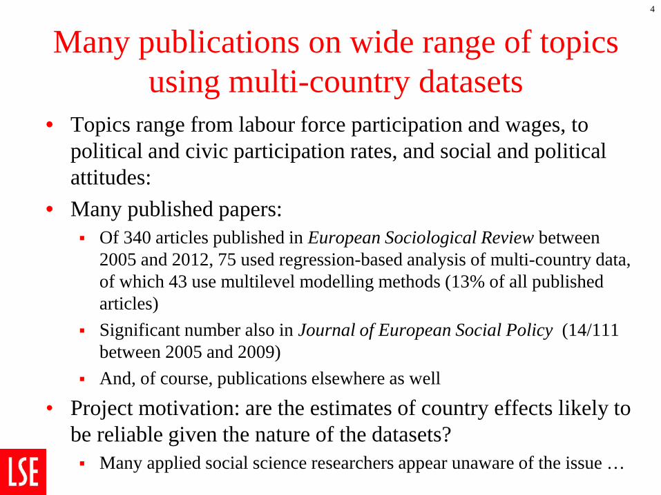
• Topics range from labour force participation and wages, to political and civic participation rates, and social and political attitudes:

• Many published papers: Of 340 articles published in European Sociological Review between

2005 and 2012, 75 used regression-based analysis of multi-country data, of which 43 use multilevel modelling methods (13% of all published articles)

Significant number also in Journal of European Social Policy (14/111 between 2005 and 2009)

And, of course, publications elsewhere as well

• Project motivation: are the estimates of country effects likely to be reliable given the nature of the datasets? Many applied social science researchers appear unaware of the issue …

4

Project Output #1: Bryan and Jenkins ‘Regression analysis of country effects using multilevel data: a cautionary tale’

ISER Working Paper 2013-14 https://www.iser.essex.ac.uk/publications/working-papers/iser/2013-14

• Multilevel models (MLMs) are not the only way to analyse multi-country data We review MLM and other approaches

• MLMs can yield unreliable estimates of country effects when there is only a small number of countries in the data set (as is typically the case: see Table above)

• Our conclusions draw on Monte-Carlo analysis of linear and binary logit mixed models with 2 specifications for each: Basic: random country intercept and a country-level predictor; Extended: as (i), plus 2 random slopes and cross-level interaction

– Extended model discussed in this talk

5

This talk: Issues arising in the Monte-Carlo analysis of a binary logit mixed model

• Computational issues: my experiences and tips from using simulate, with xtmelogit and runmlwin, and post-estimation processing using e.g. parmby, and eclplot Few how-to-do-it guides for newbies; Cameron & Trivedi, Greene, ...

• Substantive issues: comparison of Stata’s default adaptive quadrature estimator (7 quadrature points) with MLwiN’s PQL2 estimator Extremely long run times for Stata (version 11) compared to

MLwiN (version 2.25) – E.g. for C = 20: Stata 19 days compared to MLwiN 1.5 hours! – Runtime problems with Stata jobs made worse: halted by Windows Update (office

PC) and unknown gremlins (LSE’s Windows server cluster used to run almost all jobs)

MLwiN very fast, but PQL2 estimators can perform poorly – ‘Well-known’? … but only a few previous results (Rodriquez & Goldman 2001,

Pinheiro & Chao 2006, Austin 2010), and not for the data structure of interest here

6

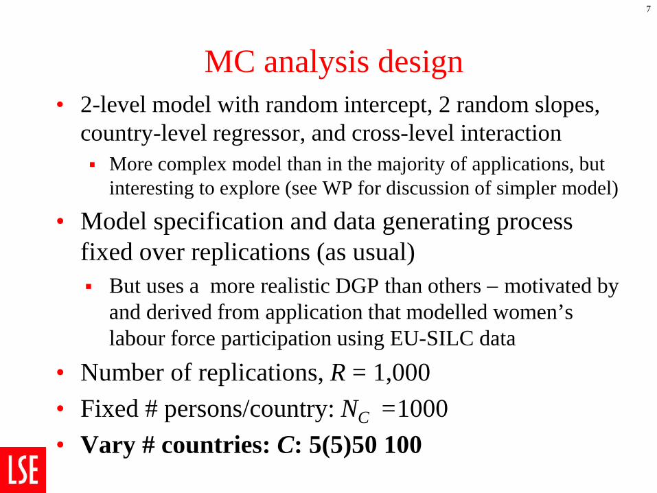
MC analysis design • 2-level model with random intercept, 2 random slopes,

country-level regressor, and cross-level interaction More complex model than in the majority of applications, but

interesting to explore (see WP for discussion of simpler model)

• Model specification and data generating process fixed over replications (as usual) But uses a more realistic DGP than others − motivated by

and derived from application that modelled women’s labour force participation using EU-SILC data

• Number of replications, R = 1,000 • Fixed # persons/country: NC =1000 • Vary # countries: C: 5(5)50 100

7

Monte-Carlo analysis: DGP reflects an EU-SILC application

• Data on women aged 18−64 years from EU-SILC cross-section for 2007 (26 countries)

• Logit model of probability of participation in labour market, as functions of individual-level: age, age-squared, marital status (binary), number of

children (integer), education level (4 categories derived from ISCED) country-level: total childcare and pre-primary spending as a % of GDP

(continuous) • DGP: (a) baseline parameters derived from preliminary estimates

of each of models (i) and (ii) • DGP: (b) joint distribution of the regressors derived using a cell-

based approach Combinations of regressors define cells; Pr(individual in cell) derived

from empirical frequency distribution in EU-SILC estimation samples Age distribution fitted as Singh-Maddala for model (i), and uniform for

model (ii) in EU-SILC data. Parameters used to generate age values that were then grouped into 5 classes in order to construct the cells

• DGP is same for each model examined; MC design varies C

8

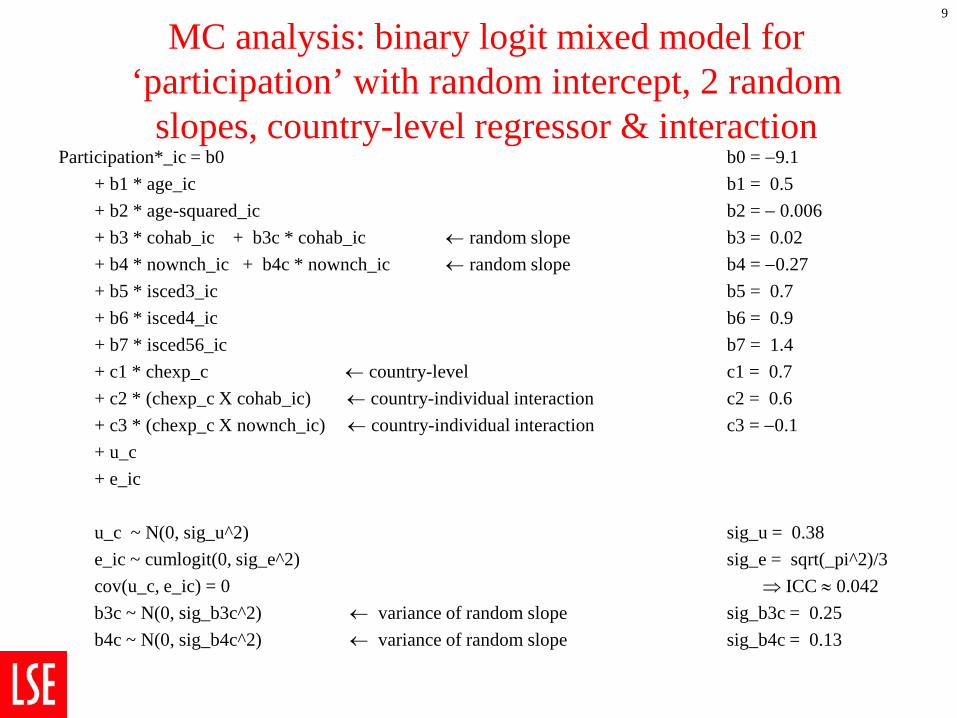
MC analysis: binary logit mixed model for ‘participation’ with random intercept, 2 random

slopes, country-level regressor & interaction

9

Participation*_ic = b0 + b1 * age_ic + b2 * age-squared_ic + b3 * cohab_ic + b3c * cohab_ic ← random slope + b4 * nownch_ic + b4c * nownch_ic ← random slope + b5 * isced3_ic + b6 * isced4_ic + b7 * isced56_ic + c1 * chexp_c ← country-level + c2 * (chexp_c X cohab_ic) ← country-individual interaction + c3 * (chexp_c X nownch_ic) ← country-individual interaction + u_c + e_ic u_c ~ N(0, sig_u^2) e_ic ~ cumlogit(0, sig_e^2) cov(u_c, e_ic) = 0 b3c ~ N(0, sig_b3c^2) ← variance of random slope b4c ~ N(0, sig_b4c^2) ← variance of random slope

b0 = −9.1 b1 = 0.5 b2 = − 0.006 b3 = 0.02 b4 = −0.27 b5 = 0.7 b6 = 0.9 b7 = 1.4 c1 = 0.7 c2 = 0.6 c3 = −0.1 sig_u = 0.38 sig_e = sqrt(_pi^2)/3 ⇒ ICC ≈ 0.042 sig_b3c = 0.25 sig_b4c = 0.13

Stata 11‘driver’ program (extract): NC and C are arguments

set seed 123456789

<material omitted, including data generation>

program define mc_silc

version 11

args sig_e sig_u sig_b3c sig_b4c

capture drop y u_c b3c b4c e_ic

gen e_ic = rnormal(0,`sig_e')

gen u_c = rnormal(0, `sig_u') if tag

bys country_id : replace u_c = u_c[1]

gen b3c = rnormal(0, `sig_b3c') if tag

bys country_id: replace b3c = b3c[1]

gen b4c = rnormal(0, `sig_b4c') if tag

bys country_id: replace b4c = b4c[1]

ge y = cond(fixed + u_c + b3c*cohab + b4c*nownch + e_ic > 0, 1, 0 )

// default estimation method is used (adaptive quadrature; 7 points), cov structure independent

xtmelogit y age agesq cohab nownch isced3 isced4 isced56 ///

chexp chexpXcohab chexpXnownch || country_id: cohab nownch , nolog iter(250)

end

di "Time is: " c(current_time) " on " c(current_date)

simulate _b _se converged = e(converged) logRLL = e(ll) ///

, reps(1000) saving(mc_hours_model3_v01_`Nc'_`C'_output.dta, replace double every(10)) ///

: mc_silc (`sig_e') (`sig_u') (`sig_b3c') (`sig_b4c')

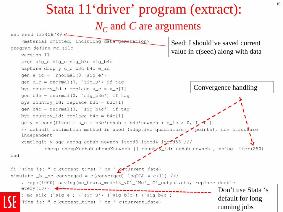
di "Time is: " c(current_time) " on " c(current_date)

10

Seed: I should’ve saved current value in c(seed) along with data

Convergence handling

Don’t use Stata ‘s default for long- running jobs

Lessons regarding doing MC analysis (the benefits of hindsight)

1. Save convergence status along with simulation output 2. Save simulation estimation frequently if runtimes are

long 3. Save current value of seed along with data, in case

wish to restart from where stopped Bill Gould’s messages on Statalist

4. Think very seriously about how to split the MC analysis into smaller ‘packages’ (blocks of replications), and combining simulation output once all blocks have run Stas Kolenikov’s messages on Statalist

11

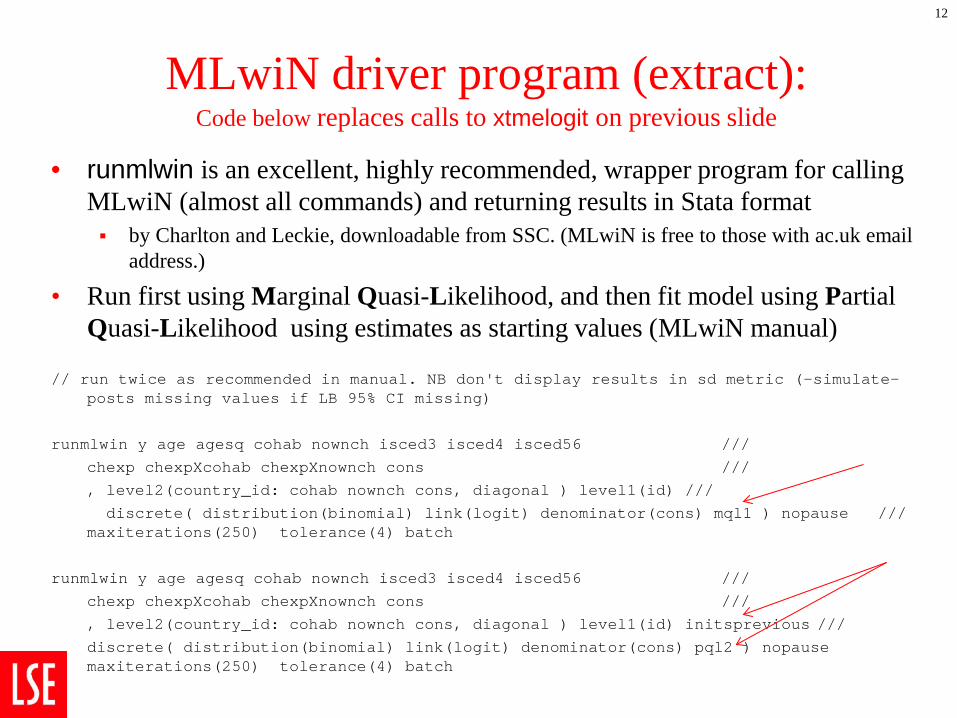
MLwiN driver program (extract): Code below replaces calls to xtmelogit on previous slide

• runmlwin is an excellent, highly recommended, wrapper program for calling MLwiN (almost all commands) and returning results in Stata format by Charlton and Leckie, downloadable from SSC. (MLwiN is free to those with ac.uk email

address.)

• Run first using Marginal Quasi-Likelihood, and then fit model using Partial Quasi-Likelihood using estimates as starting values (MLwiN manual)

// run twice as recommended in manual. NB don't display results in sd metric (-simulate- posts missing values if LB 95% CI missing)

runmlwin y age agesq cohab nownch isced3 isced4 isced56 ///

chexp chexpXcohab chexpXnownch cons ///

, level2(country_id: cohab nownch cons, diagonal ) level1(id) ///

discrete( distribution(binomial) link(logit) denominator(cons) mql1 ) nopause /// maxiterations(250) tolerance(4) batch

runmlwin y age agesq cohab nownch isced3 isced4 isced56 ///

chexp chexpXcohab chexpXnownch cons ///

, level2(country_id: cohab nownch cons, diagonal ) level1(id) initsprevious ///

discrete( distribution(binomial) link(logit) denominator(cons) pql2 ) nopause maxiterations(250) tolerance(4) batch

12

Post-processing of simulation output 1. append simulation output produced for each value of C 2. Derive various summary statistics from the output,

including relative bias, and coverage rates mean …, over(C), followed by getmata, Mata calculation of

summary statistics based on e(b) and e(V), putmata to return to Stata .dta files, listed, and also sent to rtf files for tabular summaries (using mkmat and Ben Jann’s esttab on SSC)

3. Accompanying processing to produce summary graphs: the joys of parmby and eclplot (by Roger Newson, on SSC)

parmby "mean b_cons_noncover b_age_noncover b_agesq_noncover b_cohab_noncover b_nownch_noncover b_isced3_noncover b_isced4_noncover b_isced56_noncover c_chexp_noncover c_chexpXcohab_noncover c_chexpXnownch_noncover sig_u_noncover sig_b3c_noncover sig_b4c_noncover icchat_noncover " ///

, by(C) label saving(summary_partic_model3_s_ncover.dta, replace)

eclplot estimate min95 max95 C if parm == "sig_u_noncover" /// , xlab(5(5)50 100) ylab(0(.02).4, angle(0) format(%03.2f) ) ///

yline(0.05) ymtick(0(.01).4) ytitle("Non-coverage rate")

13

Summarising MC analysis • Relative parameter bias: percentage difference between

estimated parameter and true parameter, averaged over R replications Ideal reference point: 0%

• Non-coverage rate: calculate 95% CI for each estimated parameter, assuming normality; calculate non-coverage indicator variable set equal to 0 if the CI included the true parameter, 1 if did not. Non-coverage rate is average over R replications Ideal non-coverage rate for 95% CI is 0.05 Rates larger than 0.05 mean estimated CI is too narrow

• Charts to follow show estimates of above and 95% CI (summarising simulation variability)

• Look at 2 things: Stata versus MLwiN; performance relative to typical C (around 25 in multicountry datasets)

• For brevity, selected estimates only!

14

Relative parameter bias, b_age

Stata AQ

MLwiN PQL2

15

-10

-8

-6

-4

-2

0

2

4

6

8

10

Rel

ativ

e bi

as (%

)

5 10 15 20 25 30 35 40 45 50 100Number of countries

b_age

-10

-8

-6

-4

-2

0

2

4

6

8

10

Rel

ativ

e bi

as (%

)

5 10 15 20 25 30 35 40 45 50 100Number of countries

b_age

Individual fixed effect [Similar results for most other individual fixed effects

and for individual-level variance]

Relative parameter bias, b_cohab

Stata AQ

MLwiN PQL2

16

-200-180-160-140-120-100-80-60-40-20

020406080

100

Rel

ativ

e bi

as (%

)

5 10 15 20 25 30 35 40 45 50 100Number of countries

b_cohab

-200-180-160-140-120-100-80-60-40-20

020406080

100

Rel

ativ

e bi

as (%

)

5 10 15 20 25 30 35 40 45 50 100Number of countries

b_cohab

Individual fixed effect for which there’s also cross-level interaction: note large degree of simulation variability

Relative parameter bias, c_chexp

Stata AQ

MLwiN PQL2

17

-10-8-6-4-202468

101214161820

Rel

ativ

e bi

as (%

)

5 10 15 20 25 30 35 40 45 50 100Number of countries

c_chexp

-10-8-6-4-202468

101214161820

Rel

ativ

e bi

as (%

)

5 10 15 20 25 30 35 40 45 50 100Number of countries

c_chexp

Country-level fixed effect

Relative parameter bias, c_chexpXcohab

Stata AQ

MLwiN PQL2

18

Cross-level interaction

-10-8-6-4-202468

101214161820

Rel

ativ

e bi

as (%

)

5 10 15 20 25 30 35 40 45 50 100Number of countries

c_chexpXcohab

-10-8-6-4-202468

101214161820

Rel

ativ

e bi

as (%

)

5 10 15 20 25 30 35 40 45 50 100Number of countries

c_chexpXcohab

Relative parameter bias, sig_b3c

Stata AQ

MLwiN PQL2

19

-60-55-50-45-40-35-30-25-20-15-10-505

10

Rel

ativ

e bi

as (%

)

5 10 15 20 25 30 35 40 45 50 100Number of countries

sig_b3c

-60-55-50-45-40-35-30-25-20-15-10-505

10

Rel

ativ

e bi

as (%

)

5 10 15 20 25 30 35 40 45 50 100Number of countries

sig_b3c

Random slope variance

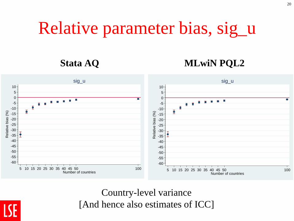
Relative parameter bias, sig_u

Stata AQ

MLwiN PQL2

20

-60-55-50-45-40-35-30-25-20-15-10-505

10

Rel

ativ

e bi

as (%

)

5 10 15 20 25 30 35 40 45 50 100Number of countries

sig_u

-60-55-50-45-40-35-30-25-20-15-10-505

10

Rel

ativ

e bi

as (%

)

5 10 15 20 25 30 35 40 45 50 100Number of countries

sig_u

Country-level variance [And hence also estimates of ICC]

Non-coverage rate, b_age

Stata AQ

MLwiN PQL2

21

0.00

0.02

0.04

0.06

0.08

0.10

0.12

0.14

0.16

0.18

0.20

Non

-cov

erag

e ra

te

5 10 15 20 25 30 35 40 45 50 100Number of countries

b_age

0.00

0.02

0.04

0.06

0.08

0.10

0.12

0.14

0.16

0.18

0.20

Non

-cov

erag

e ra

te

5 10 15 20 25 30 35 40 45 50 100Number of countries

b_age

Individual fixed effect [Similar results for most other individual fixed effects

and individual-level variance]

Non-coverage rate, b_cohab

Stata AQ

MLwiN PQL2

22

0.00

0.02

0.04

0.06

0.08

0.10

0.12

0.14

0.16

0.18

0.20

Non

-cov

erag

e ra

te

5 10 15 20 25 30 35 40 45 50 100Number of countries

b_cohab

0.00

0.02

0.04

0.06

0.08

0.10

0.12

0.14

0.16

0.18

0.20

Non

-cov

erag

e ra

te

5 10 15 20 25 30 35 40 45 50 100Number of countries

b_cohab

Individual fixed effect for which there’s also cross-level interaction

Non-coverage rate, c_chexp

Stata AQ

MLwiN PQL2

23

0.000.020.040.060.080.100.120.140.160.180.200.220.240.260.280.30

Non

-cov

erag

e ra

te

5 10 15 20 25 30 35 40 45 50 100Number of countries

c_chexp

0.000.020.040.060.080.100.120.140.160.180.200.220.240.260.280.30

Non

-cov

erag

e ra

te

5 10 15 20 25 30 35 40 45 50 100Number of countries

c_chexp

Country-level fixed effect

Non-coverage rate, c_chexpXcohab

Stata AQ

MLwiN PQL2

24

Cross-level interaction

0.00

0.02

0.04

0.06

0.08

0.10

0.12

0.14

0.16

0.18

0.20

Non

-cov

erag

e ra

te

5 10 15 20 25 30 35 40 45 50 100Number of countries

c_chexpXcohab

0.00

0.02

0.04

0.06

0.08

0.10

0.12

0.14

0.16

0.18

0.20

Non

-cov

erag

e ra

te

5 10 15 20 25 30 35 40 45 50 100Number of countries

c_chexpXcohab

Non-coverage rate, sig_b3c

Stata AQ

MLwiN PQL2

25

0.000.020.040.060.080.100.120.140.160.180.200.220.240.260.280.30

Non

-cov

erag

e ra

te

5 10 15 20 25 30 35 40 45 50 100Number of countries

sig_b3c

0.000.050.100.150.200.250.300.350.400.450.500.550.600.650.70

Non

-cov

erag

e ra

te

5 10 15 20 25 30 35 40 45 50 100Number of countries

sig_b3c

Random slope variance Note different scales, LHS and RHS

Non-coverage rate, sig_u

Stata AQ

MLwiN PQL2

26

0.000.020.040.060.080.100.120.140.160.180.200.220.240.260.280.300.320.340.360.380.40

Non

-cov

erag

e ra

te

5 10 15 20 25 30 35 40 45 50 100Number of countries

sig_u

0.000.050.100.150.200.250.300.350.400.450.500.550.600.650.70

Non

-cov

erag

e ra

te

5 10 15 20 25 30 35 40 45 50 100Number of countries

sig_u

Country-level variance [And hence also estimates of ICC]

Note different scales, LHS and RHS

Conclusions • Computational (1): Lessons about how to implement Monte-

Carlo analyses using Stata • Computational (2): Stata 13’s speedier mixed logit model

estimators will help! • Substantive (1): general problem of reliability of estimates

when one has multi-country data with small number of countries Apparently not realised by many applied social scientists

• Substantive (2): Adaptive quadrature performs better than PQL for mixed binary logit models, notably for random effect variances

• Substantive (3): Would be useful to explore other (less familiar) approaches to estimation and inference, e.g. … Bayesian approach (e.g. MCMC in MLwiN, BUGS)

– Does relatively well in the small-C case, suggests research by Browne & Draper (2006), Moineddin et al. (2007), Stegmuller (2013)

27