TECHNICAL REPORT SECTIONNAV&L POSTGRADUATE SCHOOlMOM i EfvEY. CALirOstMIA 93940
NPS55Lw75061
NAVAL POSTGRADUATE SCHOOL
Monterey, California
A MOVING AVERAGE EXPONENTIAL POINT PROCESS (EMA1)
-by
A. J . Lawrance
and
P. A. W. Lewis
June 1975
Approved for public release; distribution unlimited,
r
FEDDOCSD 208.14/2:
NPS-55LW75061
NAVAL POSTGRADUATE SCHOOLMonterey, California
Rear Admiral Ishara Linder
.
Jack R. BorstingSuperintendent Provost
The work reported herein was supported in part by the Office of NavalResearch, the National Science Foundation and the United Kingdom ScienceResearch Council.
Reproduction of all or part of this report is authorized.
Prepared by:
UNCLASSIFIEDSECURITY CLASSIFICATION OF THIS PAGE (Whan Data Entered)
REPORT DOCUMENTATION PAGE READ INSTRUCTIONSBEFORE COMPLETING FORM
1. REPORT NUMBER
NPS55Lw75061
2. GOVT ACCESSION NO 3. RECIPIENT'S CATALOG NUMBER
4. TITLE (and Subtitle)
A Moving Average Exponential Point Process(EMA1)
5. TYPE OF REPORT ft PERIOD COVERED
Technical Report
6. PERFORMING ORG. REPORT NUMBER
7. AUTHORC*,)
A. J. LawranceP. A. W. Lewis
8. CONTRACT OR GRANT NUMBERCs)
9. PERFORMING ORGANIZATION NAME AND ADDRESS
Naval Postgraduate SchoolMonterey, California 93940
10. PROGRAM ELEMENT, PROJECT, TASKAREA ft WORK UNIT NUMBERS
II. CONTROLLING OFFICE NAME AND ADDRESS 12. REPORT DATE
June 197513. NUMBER OF PAGES
U. MONITORING AGENCY NAME ft ADDRESSf// different from Controlling Office) 15. SECURITY CLASS, (of thla report)
Unclassified
15a. DECLASSIFI CATION/ DOWN GRADINGSCHEDULE
16. DISTRIBUTION ST ATEMEN T (of thla Report)
Approved for public release; distribution unlimited
17. DISTRIBUTION STATEMENT (of the abatracl entered In Block 20, It different from Report)
18. SUPPLEMENTARY NOTES
19. KEY WORDS (Continue on reverae aide If neceaaary and Identify by block number)
Linear CombinationsPoisson ProcessMoving Average
Point ProcessRandom SequenceVariance Time Curve
20. ABSTRACT (Continue on reverae aide If neceaaary and Identify by block number)
A construction is given for a stationary sequence of random variables{X.} which have exponential marginal distributions and are random linearcombinations of order one of an i.i.d. exponential sequence {e.}. Thejoint and trivariate exponential distributions of X > X. and X. -
are studied, as well as the intensity function, point spectrum and variancetime curve for the point process which has the {X.} sequence for successive
DD 1 JAN 73 1473 EDITION OF 1 NOV 65 IS OBSOLETES/N 0102-014-6601
|
UNCLASSIFIEDSECURITY CLASSIFICATION OF THIS PAGE (Whan Data Bntarad)
UNCLASSIFIED
.bCUWTY CLASSIFICATION OF THIS PAGErWh-. D'tm Ent.r.d)
times between events. Initial conditions to make the point process count
stationary are given, and extensions to higher order moving averages and
Gamma point processes are discussed.
UNCLASSIFIEDSECURITY CLASSIFICATION OF THIS PAGEfWh.n D.f- Enf.r.*
A MOVING AVERAGE EXPONENTIAL POINT PROCESS (EMA1)
A. J. LawranceUniversity of Birmingham
England
and
P. A. W. LewisNaval Postgraduate SchoolMonterey, California
ABSTRACT
A construction is given for a stationary sequence of random variables
{X.} which have exponential marginal distributions and are random linear
combinations of order one of an i.i.d. exponential sequence {e.}. The joint
and trivariate exponential distributions of X. , , X. and X... are studied,i-l i l+l
as well as the intensity function, point spectrum and variance time curve for
the point process which has the {X.} sequence for successive times between
events. Initial conditions to make the point process count stationary are
given, and extensions to higher order moving averages and Gamma point processes
are discussed.
1. Introduction
In this paper we discuss the stationary sequence of random variables
{X.} which are formed from an independent and identically distributed
exponential sequence {e.} according to the linear model
*Support from the Office of Naval Research (Grant NR042-284) , the National
Science Foundation (Grant AG476) and the United Kingdom Science ResearchCouncil is gratefully acknowledged.
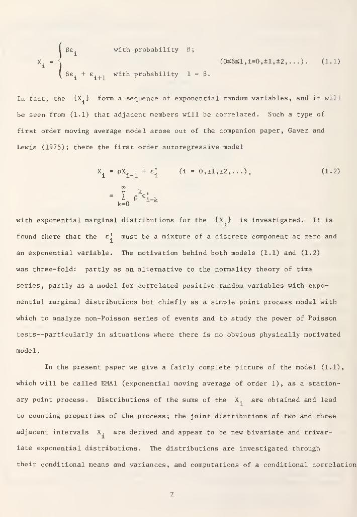
!e . with probability 3;1
(O£0£l,i=O,±l,±2,...). (1.1)
.th probability 1-3.'1_
)I Be. + z wilv l l+l
In fact, the {X.} form a sequence of exponential random variables, and it will
be seen from (1.1) that adjacent members will be correlated. Such a type of
first order moving average model arose out of the companion paper, Gaver and
Lewis (1975); there the first order autoregressive model
Xi
= pXi-l
+ Ei
(i = 0,±1,±2,...), (1.2)
00
" ^ P i-kk=0
X *
with exponential marginal distributions for the {X.} is investigated. It is
found there that the e! must be a mixture of a discrete component at zero and
an exponential variable. The motivation behind both models (1.1) and (1.2)
was three-fold: partly as an alternative to the normality theory of time
series, partly as a model for correlated positive random variables with expo-
nential marginal distributions but chiefly as a simple point process model with
which to analyze non-Poisson series of events and to study the power of Poisson
tests—particularly in situations where there is no obvious physically motivated
model.
In the present paper we give a fairly complete picture of the model (1.1),
which will be called EMA1 (exponential moving average of order 1), as a station-
ary point process. Distributions of the sums of the X. are obtained and lead
to counting properties of the process; the joint distributions of two and three
adjacent intervals X. are derived and appear to be new bivariate and trivar-
iate exponential distributions. The distributions are investigated through
their conditional means and variances, and computations of a conditional correlation
are given. Extensions of the model and estimation problems are briefly
discussed.
In developing the properties of the process we will also point out
similarities to a backward first order moving average which is defined as
[Be. + E. . wiiV 1 l-l
Be. with probability B,
(O£0£l;l-O t ±l,±2,...) . (1.3)
th probability 1 - B.
Properties of the processes are very similar, but those of the forward
model (1.1) have simpler derivations.
It should also be noted that the model (1.1) can be written as a very
special type of linear model with random coefficients:
X. = Be. + I.e (O^B^l, i = 0,±1,±2,...)
,
where the I. are i.i.d. Bernoulli random variables which are 1 withl
probability 1-B and with probability B. This characterization is not
very helpful for the first order model; the main point is that since the
random coefficient has a probability which is just the parameter B, many
of the theorems for linear processes are not applicable.
2. Some Basic Aspects of the EMA1 Model
The simplest aspect of the EMA1 model is the exponential marginal
distribution of the intervals (X.}; in point process terminology (see e.g.
Lawrance, 1972) this is the synchronous distribution of intervals and refers
to the distribution of the interval from an arbitrarily chosen event to the
next event. For the Laplace transform of its probability density function
(p.d.f.) f (x) , we writeA •
1
* -sX.
fx
(s) = E{eX
}
i
-s$e. -s8e.-se= E{e
1)B+ E(e
X X i}(l-B) (2.1)
using (1.1). Now the i.i.d. random variables e. have exponential distributions
with parameters X, say, and so their Laplace transform is X/(A+s). Thus
(2.1) becomes
fx.<
s) -d5r B + x3T»s-<1-,) -&i
This demonstrates that the X. have identical exponential distributions as
asserted. The parameter X is thus the number of events per unit time, or
the rate of the point process.
The correlation between X. and X. M is easily obtained on consid-l l+l
ering the product of X. from (1.1) with
xi+i
[$e with probability 6,
'3e.+1
+ e. +2with probability (1-3)
Thus, again using straightforward conditioning arguments,
CX.X.,.) = FJBe.r )B 2
UB^.e.^e.e.+2
)B(l-B)
Ef6 2 e.e. J_.4-Be2 )B(l-6)
E(^ e. Ei^ £
. ei+2^. +ie . +2+Bc21+1
)(l-B)2,
and simplification of this result leads to
±= corr(X
i,X.
+1 ) = B(l-B). (2.2)
By the construction of EMA1, the higher order serial correlations will be zero,
and thus the spectral density of intervals (Cox and Lewis, 1966, p. 70),
fM (ta) - — {1*2 I o cos(kaj)}, (O^u^tt),
71
k=lk
becon ~
f.(u) - - {1 + 2S(l-8)cos(0))}. (O^oxtt). (2.3)
The result (2.2) is the greatest limitation of the EMA1 model since it implies
that the first order serial correlation is non-negative and bounded by 1/4;
this may be compared with an ordinary MAI model assuming two-sided e . dis-
tributions of mean zero for which |p1
|£ 1/2. In both cases it can be
anticipated that the restrictions are a consequence of the linearity of the
models
.
A further simple aspect of the EMA1 model is that the {X.} sequencel
reduces tc the Poisscr process when B = or 1, and this gives checks on
most of our results. We mav also note that the moving average is taken in the
forward sense ; t:he backward model (1.3) could equally have been treated,
although producing different but similar results. This serves to emphasize
that there is no time-reversibility in the process, in the sense that
{Xn
, . . .,X } does not have the same joint probability distribution as
{X , , . . . ,X , } for all finite k, where k > 2
.
-1 -k —
3. Distributions of Sumr; and Counts jr. (x } Sequence
In the point process theory of the model, the distribution of the sums
T = X,-4-. . .+X are very useful; if these can be obtained then the distribu-r 1 r
tions of counts, both in the synchronous and asynchronous mode, can then be
derived. \s shown in Cox and Lewis (1966, Chapter 4) for instance, these
then .lead to the second order properties such as the intensity function, the
(Bartlett) soectrum of counts and the variance time curve. It is, therefore,
a particularly attractive feature of the EMA1 model that the distribution of
the T may be obtained, and we shall now give a simple derivation.
Define i>(s) as the Laplace transform of the p.d.f. of the e. distri-i
bution: except where otherwise remarked this distribution is exponential of
parameter X ar ' so il^(s) = X/(A+s). Define the rouble Laplace transform
I equivalently the joint moment generating function) of T and e.
-,> as
-s T -s_e4
T.(s
1,s ) = E(e
L r l r L} for r = 1,2,... . (3.1)
For : = 1, we have
-s X -s e -s Be -s e -s Be -(s +s )e
i.(s.,sj= E(eL X A 2
} = E{eL l l 2
}8 + E(eX 1 L l 2
}(1-B)1 z
= t!;(BSi )[BHi(s 2) + (l-B)^( Sl+s 2
)] (3.2)
and we shall write
JH'sr s2
) = BiJj(s2
) + (1-B)i|;(s +s ). (3.3)
This is the double Laolaco transform of a joint distribution in which the
first iriable has mass B at zero and with probability (1-B) is exponen-
tial distributed. We shall now relate <}> (s ,s ) and cj> .(s1,s„). Since
T = T . + Xr r-1 r
T , + Be with probability 3r-1 r
T , + Be + e , , with probability 1-3,r-1 r r+1
we have
-S..T , -s.pe -s_e -s.T ,-s.Be -(s.+s )e
r(8r 8
2) - E(e
lr"! !r 2r - 1
}3 + E{eX r"1
*r X 2 r+1
}(l-3)
= 4>
r_ 1(s
1,3s
1)iJ;(s
2)3 + 4.
r_ 1(s
1,3s
1)^(s
1+s
2)(l-B)
= [B*(a2) + (l-3)«(s
1+s
2)]«
r_1(8
1,3s
1). (3.4)
Solving (3.4) gives,
4>
r(s
1,s
2) = *(B8
1)[«(s 1> Bs1
)]r"1
*(slt a2),(3.5)
and setting s = 0, we have for the Laplace transform of the p.d.f. of T ,
*r(s) = [3<K3s) + (1-B)iKBsWs)][BiKBs) + (1-B)i|»((l+B)s) ]
r_1(3.6)
X(A+23s)X+s (a+23s){X+(l+3)s] } , r * 1, (3.7)
This is our required result; from (3.7) it will be observed that T is dis-
tributed like the sum of r independently distributed variables, such as in
a delayed renewal process, although these are not X variables. The structure
of (3.6) or (3.7) is explained by the fact that the number of intervals which
are of the 3e. form or Be. + e.,-, form are binomially distributed with1 x 1+1
parameter B or 1-3; further consideration of the adjacencies of the two
types of intervals than leads to the terms in the binomial expansion of (3.6) .
We now obtain the distribution of N , the synchronous counting process
of number of events occurring in the interval (0,t] beginning at an arbitrary
event; this is related to the distribution of T through the equivalence of
the events N < r and T > t for r i 1. Let F (t) denote the distri-t r r
burin- of T , and then sincer
Prob{N[f)
= r} = Fr(t) - F^Ct), r ^ 0, (3.8)
with F (t) = 1 for t 2> 0, we have for the p.d.f. of N ,
N °°
E{zt
} m * ( Z ;t) - I zr[F
r(t) - F (t)]
r=0
oo
- 1 + (z-1) I zr_1
F (t). (3.9)r=l
r
Inserting (3.7) in the Laplace transform of (3.9) gives
* , m B(l+B)s 2 + [-B(l-B)z-*-2B+l]As + X 2 .
"f;
(s-"-X)l6(l+B)s ;: + (l+2B-2Bz)As + (l-z)A 2]
U--"^
This result is required in Section A to follow.
4. The Intensity Function and Spectrum of Counts
The intensity function of a point process is the derivative with
respect to t of E{N } and will be denoted by m (t) . The (Bartlett)
spectrum of counts, the Fourier transform of the covariance density of the
differential counting process, then has the simple expression
8+(w) = ^ {1 + m*(iu>) + m*(-iu))}, (4.1)
where m (s) is the Laplace transform of mf (t); this expression for g,(w)
is derived in Cox and Lewis (1966, Section 4.5).
For the EMA1 process, the result from (3.10) is that
m*(*\ - X(A+gs){A+(l+g)sj[(L on
fvs;
' 8(l+B)s(X+s){s+X/(8 z+B)}' K ]
In inverting the Laplace transform (4.2) it will be noted that the
case 3+3=1, i.e. 3 - 0.6185, must be treated separately since there
will then be a factor (X+s) 2 in the denominator. Partial fraction expansions
and their inversion then give, for t ^ 0,
mf(t) = ^ +f^ {e"
Xt/(e2+B)- e~
Xt] (B*W1). (4.3)
= Atl + 33Xte"
Xt] (3
2+3=l). (4.4)
We see in both cases that the initial value of m (t) is X and that they
both increase until maximum values are obtained at t = X (B2^) x log[(3 2+3)/
(32+3~l) ] and at t = X respectively for (4.3) and (4.4); both functions
then decrease exponentially to X. There is no apparent reason for the
3+3=1 case. When 8=0 or 1 both functions are constant at X, as
is appropriate to the Poisson process.
10
The function m (t) is plotted in Figure 1 for several values of 8.
The spectrum of count? follows easilv by inserting (4.2) into (4.1), and has
the expressions
( \ Mt± -m? 6(1-6) f g2+B 1
~\\ , fl2xcin ( , ,,
gj>) - - ^1 -f 2A 2 ^^'L(e„6)y^2 " T^TtJ) (6
2+6*l) (4.5)
(62+6=l). (4.6)
We observe that both these are ratios of 4th order polynomials in u). Esti-
mation of both m (t) and g^(w) given an actual sequence of interevent times
is considered in Cox and Lewis (1966, Chapter 5); in practice these would then
be compared with our given theoretical functions which are graphed in Figure 2.
Note that unlike the 2nd order -joint moment functions p, and f,(w)— k +
for intervals, the second order moment functions for counts mJ.(t) and g, (co)t +
do discriminate between the cases where the parameter is 3 or (1-6)
.
tiowp ,,n.r the graphs in Figure 2 indicate that the count spectra of models with
6 in the ranee (0.25. 0.75) are fairly close to each other; therefore, the
spectrum will not be entirely suitable for discriminating between different
6 values for small sample sizes.
The variance time curve is considered in Section 7, along with the
stationary initial conditions for the process.
11
5. The Joint Distribution of X. and X. inx 1+1
We now discuss the joint distribution of X. and X. in which willJ 1 l+l
be a bivariate exponential distribution. Several authors have discussed bivar-
iate exponential distributions, including Downton (1970), who makes some compari-
sons with those of Gumbel, Moran and Marshall-Olkin . The distribution to be
discussed here does not appear to be one of the earlier ones, although it is
fair to say that in common with earlier ones, it is not the 'perfect' bivariate
exponential.
The double Laplace transform of the joint pdf of X. and X is
easily calculated using (1.1); the required expectation is
„."SlVS
2Xi+l, **
E{e } = £x.,x. <
sr s 2>1 1+1-3s..e.-3s „e -Bs.e.-s (Be +E )
=E{e lx 2l+1}3
2 +E{e lx 2 1+1 1+2}3(l-3)
-s- (3e.+£. .-J-as-e..,+E{e 1 i i+l 2 i+l
}B(1_g)
-s (3e.+e )-s (Be +e )
+E{e 1 i i+l 2 i+l i+2}(1_e)
2} (5#1)
which can be written
fX X
(s1,s
2) = ij;(3s
1)[3'P(3s
2)+(l-3)^(s
1+3s
2)][3+(l-3)^(s
2)] (5.2)
i' i+l
X 2 (X+3s1+3s
2)
(X+3s1)(X+s
2)(X+s
1+3s
2)
* (5.3)
We note that (5.3) is not symmetrical in s and s_, and this is to be
expected since the process is not time reversible; this is one feature which
distinguishes it from earlier bivariate exponentials. The backward moving
average model (1.3) corresponding to (1.1) has the joint interval distribution
which is specified by (4.3) with s and s interchanged.
12
An explicit form of the joint distribution (5.3) can be obtained
directly, rather than by inversion of the transform which is less
informative. By the structure of the model the joint distribution of (X..X.,,)i l+l
is a mixture of the joint distributions of (Be .,8e ) ,
(Be . ,Be +e )
,
(Be . -*«..- ,Be ._._) and (Be .-K Be +e ) with the corresponding probabili-1 l+l l+l l l+l l+l i+2 & r
ties B2
, 8(1-6), 6(1-8) and (1-6) 2. These joint pdf's can be listed in
an obvious notation as follows:
f _ (x,y) = (X/8)e-(>/S)x
(A/6)e-(A/6)^ (x,y>0)
fcs£ . ,fcsei i+1
fflp PF +F (x,y) - Xe-
Xx(l-B)-
1[Xe-
Xy-Xe-
(X/B)y], (x,y>0)
ec . , tie . _+e . _i i-1-! i+2
Be. -•-£.,., Be...i i+I i+I
(x.y) - a/8)e-<X/B)(*-y/6
>(X/B>e-(X/B)y
, (6x>y>0)
Cei i+l
,t5ei+l'
ei+2
(x.y) = <
2e-(X/6)x
[eX(l-6)y/8 2
_e-Xy
]/(1_ 6+62)) (gx>y>0)
JA2[e
-X(l-6)x_e-(X/6)x
]e-Xy
/(1_ e+62) (y>6x>0). (5.4)
We thus see that the joint pdf of X. ,X..
, will be continuous in both variablesl i+I
but will have different analytical expressions over the regions Qx > y and
Bx <_ v ; there appears to be no compact analytical form for f (x,y) .
x.,x.+1
This is unfortunate because it makes it difficult to derive maximum likelihood
estimates of the parameters \ and B in the model.
13
Different bivariate exponentials also can be compared through
their conditional properties and so we will derive these for the present
distribution. Conditional pdf's are not succinct enough, and so we
concentrate on conditional moments. These may be obtained from (5.3). For
instance, to obtain E(X. |X._=t) we differentiate with respect to s~, set
s_ = 0+, invert with respect to s and then divide by the marginal (exponen-
tial) density of X. The two conditional means are in this way found to be
E(X.|Xi_ 1
=t) = X'h^t + ^| +^ e-X(1-e)t/B
] (5.5)
and
E(X.|x.+1
=t) = X"1[l+B-e"
(1_e)Xt/B]. (5.6)
Thus, both regressions have exponential components; this property is shared by
the Marshall and Olkin bivariate distribution, although that distribution has
a singular component along X. = X . For the continuous distribution treated
by Downton both the conditional means are linear, as are the conditional
variances
.
Examining these regression functions more closely we see that E(X. |X =t)
is equal to A ' for 3=0 or 3=1; otherwise it increases exponentially
from 3X to the constant value (1+3)X " as t increases. The transient
is long for 3 close to 1, but very short when 3 is close to 0. Thus unlike
the serial correlation coefficient p, there is differentiation in this condi-
tional mean between the cases where the parameter is 3 and the case when it
has value 1-3.
The conditional mean (5.5) is more complex. It starts at t = with
value X ' and negative slope B - 1. There is a unique minimum at t =
-3 in 3/{X(l-3)} and the function eventually increases linearly with t. Since
we have for large t that
14
E[xJ xi-l
=t:] ~ x-1
Bt,
the rate of increase depends onlv on 8, not on X.
The conditional variances for the present bivariate exponential are
also exponential functions, and their explicit forms are given by
VarfX. X. = t) = A1
' l-l
-2 1-2^2^, 2B 2 (1+At) -(l-6)At/S
(1-6)^ l-B "(1-6)-2(l-B)Xt/(
(5.7)
and
Var(X. X. , =t) = Al ' l-fl
-2 l+S-!-B2-8 3
1-f_2/-A_ + At) -x(i-B)t
(1-8 B i
/B -2(1-6)A- e
t/B]. (5.8)
These conditional variances are quite different forms as shown in Figures 3
and A. In practice it is clear that conditional means and variance could only
be calculated for t in the more central regions of the marginal distributions
In these situations Var (X. X. ., ) is fairly constant, while Var(X. X #11 )i' i-l i' l+l
is reasonably linear in t. In all cases the asymptotic values are reached
much quicker for the lower value of S.
15
6. The Conditional Correlation of X , X given X±
We now wish to carry the study of dependence in the sequence of intervals
{X.} a step further, in particular to trivariate distributions. The dependence
in the EMA1 process has a very particular structure: X. is dependent on X. .. and
X but not on X._ , X , X._3> X , and so on. It thus appears that the
-joint distribution of X. ., X., X. in has some natural significance for thisJ l-l 1 l+l
process, and it will be a trivariate exponential distribution; we should note
however that in view of the coupling effect of the dependence, this trivariate
distribution is not enough to describe completely the dependence in the sequence
{X.}. In particular the sequence is certainly not Markovian since the distri-
bution of X. in |x.,X. n will depend on the value of X. ., .
l+l ' l l-l l-l
The process, by its structure, has the somewhat strange feature that
although X. n and X. in both depend on X., the variables X. .. and X., n6 l-l l+l r l l-l l+l
are independent. For this reason, it is felt that the joint distribution of
X. , and X.,- conditional on X. is of interest, and we shall give calcula-l-l l+l l
tions of the conditional correlation of X. n and X.., given X. = t. Thel-l l+l & l
other two pairwise conditional joint distributions may also of course be used,
but the corresponding unconditional joint distributions show that the intervals
concerned are not independent. We think of the conditional correlation, written
Corr(X , X. |x. = t) , as a descriptive function of the higher order dependence,
with the thought that it may be used comparatively with other trivariate
exponentials. The general properties of conditional correlations are not well
understood, but Lawrance (1975) has shown that it is equal to the corresponding
partial correlation only in very special cases, one of which is the trivariate
normal, and the present distribution is not one of these cases.
The triple Laplace transform of the joint p.d.f. of X. , , X., X... isJ r i-1 l l+l
calculated by a straightforward extension of the procedure used to obtain the
16
bivariate Laplace transform at (5.2). The result is the sum of eight expecta-
tion terms with their associated binomial probabilities, and can be cast in
the form
r
" SlXi-l~
S2Xi"
S3Xi+l^ *** , ,Ele
A\ = f (s s s )X._r X.,X.
+11 2 3
=iKBs ) (£^(es2
) + (1-6) iK S;L+6s
2)} {3^(6s
3) + (1-6) iKs
2+6s
3) *3 +U+B) iKs )}
(6.1)
This reduces to the appropriate bivariate distribtuions where one s is set to
zero. Before passing to the conditional moments, we may note that the
generalization of (6.1) to r adjacent intervals is
r r
E(exp[- Z s.X.]}= iKBs ) n IBK3s )+(l-B) iKs. ,+ s.)]Ig+(l-3) iKs)].i=l
xj=2 2 J J
(6.2)
When s, = s„ = ••• - s we recover the result for X. + X„ + • •• + X
1 2 r 1 2 r
given at (3.5).
We now return to CorrfX. , X |x. = t) which we shall denote as P~(t)i— 1 i+1 i L
the conditional correlation of X. , and X.,, given X. = t. This has thel-l l+l l
explicit expression
E(X.1,X,,.|x.=t) - E(X. . |x.=t) E(X, ,_ |X,=t)
,. 1-1 1+1' 1 1-1
' 1 1+1' 1 ,, ,v
P ?(t) = zrjz . (6.3)
[Var(X._1JX.=t) Var(X.
+1|x.=t)]
i^
In view of the results (5.5)-(5.S), there only remains to calculate
E(X. ,, X ]X.=t). This is obtained from (6.1) by inverting
17
2(x;At)_1 3i^ If
x1_rx i'
xi+i
(Sl,S2 ' S3)3(si=s
3=0) '
(6 ' 4)
as a function of s„, to recover the variable t. After subtraction of the
product of the conditional means, we have for the conditional covariance
Cov(xi-i-
xi+il
xi=t >
. - -^ + (tt-B)Xt -B> e-(1"e)Xt/B - JL .-2d-B)^t/B •
(6 . 5)1-P 1-P
Hence the expression for p 9(t) and the graphs given in Fig. 5. The conditional
correlation is far from constant in t, although in the range (0,2X), within
which it would be possible to estimate it in practice, the values are positive
and small.
18
7 . Stationary Initial Conditions
Up to this point we have dwelt on aspects of the process which involve
the intervals between the events, we have emphasized that these are a corre-
lated but stationary sequence of exponential variables. This situation is
typified by the choice of an arbitrary event for the initial point of a
sequence of intervals. We now consider the corresponding problem when the
initial point is chosen without knowledge of the event times; this is usually
called an arbitrary time and is of interest when stationarity in the counts
of events is suggested (Cox and Lewis, 1966, Chapter 4), as opposed to
stationarity in the intervals between events. However, for stationarity in
counts of events, the initial point of the interval of the counting must be
chosen in a particular probabilistic way. We shall now obtain the appropriate
initial conditions, using the approach and definition discussed in Lawrance
(1972) in which the process is considered at time t and t is then allowed
to tend to infinity. The sequence of intervals between events beginning with
the arbitrary time, usually called the asynchronous sequence, is not exponen-
tial or stationary, but the counting variable of this sequence has stationary
increments, although not Poisson distributed.
At time t in the process (after a start in any convenient way) it is
apparent that for the process to continue, we must specify:
(i) the time to the next event in the {X.} sequence, and
(ii) the random variable e.., which is associated with the end of thel+l
X. interval covering t. The first of these will be denoted by x anc* is
just the forward recurrence time of the EMAI process, and this is bound asymp-
totically to be exponential, but it will be dependent on the second, denoted
by e which will not be exponential, even asymptotically. It is their joint
distribution as t -> °° which gives the required initial conditions.
19
Suppose the process starts at t = in the synchronous mode, and
suppose that in (0,t] there are r-1 events. Let the joint pdf of T
and 3e be f„, Q (x,y). When the r— interval is of the Be form,r T ,pe r
r-1 r
then the joint pdf for (x = w, e = z) is
ft
fT Rc (x,t-x+w)dx *_ (z) ,
x=0 r-1 r
(7.1)
where i> (z) is the pdf of e . If the r— interval is of the Be + ce . r+1 r r+1
form, there are two similar expressions according as z < w or z > w; these
are
f Rc (x,t-x+w-z)dx i|> (z) (z<w)x=0 r-1 r
(7.2)
uid
t-(z-w)f
fi(x,t-x+w-z)dx ij> (z)
x=0 r-1 r
(z > w) (7.3)
The expressions become evident on considering the configuration of events
The joint pdf of x and e at time t may thus be written
00 , t
1 f „ (x,t-x+w)dx ty (z) with probabilityr=0 J x=0 r-l
,P£r
£
f (w,z;t) =X,e
oo -t
1=0 J x=0 r-1'
ooft
1
r=
00 ft-(z-w)
(x, t-x+w-z)dx \\> (z)>e er
oor t
(z<w) (7 4)
Iwith
|probability
] 1 — 8 .
f„ Q (x,t-x+w-z)dx ty (z) (z>w)r=0 J x=0 r-1 r
The r = and 1 terms here are really special cases, but will not contrib-
ute as t -* °° and do not need to be obtained explicitly. We shall now use
the result that
lim f (w,z;t) = lim sf*(w,z;s) = f (w,z)
t-*»X ' e
s-*0X,e
(7.5)
20
to obtain the limit distribution at an arbitrary time. Now for the Laplace
transform with respect to t of (7.4) we need the joint pdf of T _ and
3c , which by (3.4) is
f (x,y) = C , (x-u)k(u,y)du,r-1 r J u=0
(7.6)
and in terms of Laplace and double Laplace transforms
C*_1(s) = ^(3s)[^(s,3s)]
r 2, and k**( S;L ,s 2
) = W (Bs2
) + (1-3)^ ( Sl+Ss 2) . (7.7)
Hence the Laplace transform with respect to t of the first line of (7.4)
after ignoring the r = and r = 1 terms is
H3s)l-iKs,3s)
u=0 a=0e ' k(u,a+w)duda ty (z) (7.8)
Taking the limit as in (7.5) then gives
v^£(z)
u=0 a=0k(u,a+w)duda = vty (z) f (a+w)da = v^(w/3)4^(z) > (7.9)
a=0 M er
where v is the mean of the e distribution and ¥ (z) is its survivore
function. The limits of the other terms in (7.4) can similarly be obtained,
and give the final result as
v-1
y (w/3H (z)e e
-1
X»e
v "
^e(z)
;,w > with probability3
f (w,z) = < v "4* {(w-z)/3>^ (z) < z < w
( wi
< w < z
th probability1-3
(7.10)
21
The marginal distribution of e has pdf
fe(z) = B^(z) + (l-B)zi|»
e(z)/v. (7.11)
The marginal distribution of x is in general rather complicated, but in the
EMAI case is exponential with parameter X. From (7.11) we see that in the
EMAI case the distribution of the first e variable after an arbitrary time
(e) is the weighted sum of exponential and Erlang 2 distributions. This result
implies that the second asynchronous interval does not have the exponential
distribution, although all the following intervals do; the non-stationarity of
the asynchronous sequence of intervals is thus caused only by the second interval
The distribution for the number of events in (0,t] when t = is
an arbitrary time, that is in the stationary situation, may now be obtained
directly. As in the synchronous case of section 3 we need the distribution
t"L|
of the time to the r— event for r ^ 1. The function <}>
1(s ,s ) of section
3 is now the double Laplace transform of (7.10), and so
*1 (S1' S
2)
= vs"^^ -'Kl3 s1Mf^(s
2)+ (l-6)i|;(s
1+s
2)}]. (7.12)
Generally, for the double Laplace transform of the pdf of T and e
measured from an arbitrary event, we have as at (3.2),
*r(s
l'S2)
= <K sr s2H<Ks
1,es
1)]
r~<J,
1(s
1,6s
1) (r£2). (7.13)
This leads, using (3.9) to the Laplace transform of the pgf of N(t) as
* v S(l+3)s 2 + [-g(l-(B)z+ 28+ l]Xs+ [1+ B(l-B)z(l-z)]A 2
9 KZ ' S) (s+A){B(l+B)s z + (l+2B-28z)As+ (l-z)X z} '
K ''^ }
22
Setting 6=0 or 1 reduces this to the Poisson process result and reminds
us that the distribution of N(t) here can be considered as a generalization
of the Poisson distribution appropriate to counting events in a correlated
exponential sequence. The customary differentiations and inversions of (7.14)
give
E{N(t)} = At
and
Var{N(t)} = [l+26(l-6)]At-26(l-6)(l+3+B 2) - l^il'V [(6
2+3) 2e~At/(B +3) -e
"Xt] (7.15)
P TP-l
when 32 + 3 ^ 1; there is an individual expression for (7.15) when 6+6=1.
We notice that the distribution is asymptotically over dispersed as compared
to the Poisson distribution. The results (7.14), (7.15) may also be obtained
from general theory and the previous synchronous results, but the initial
conditions have much wider applicability.
We have then been able to explicitly obtain the main probabilistic prop-
erties of the EMA1 process in respect of stationary intervals and stationary
counts; the process is thus unusually tractable, and this is of considerable
merit as compared with many other models.
23
8. Conclusions and Extensions
There are several extensions to both the first order autoregressive
and moving average point porcesses and sequences which will be considered
subsequently:
(i) By replacing e in (1.1) with Ye.,., with probability Y
and with Y£.,, + e -,i we obtain a second order moving averagel+l i+2
process. This may be extended to any order; like the present
model the serial correlations are restricted to lie between
and 1/4.
(ii) The autoregressive and moving average structures can be combined
to give what appears to be a much richer class of processes,
(iii) In Gaver and Lewis (1975) it is shown that is the X. is taken
to be Gamma distributed (K,\) , then the solution to (1.2) shows
that e! has Laplace transform { (pX+s)/ (X+s) } and this is the
Laplace transform of an infinitely divisible distribution. Thus
autoregressive, moving average and mixed Gamma processes can be
constructed. Their properties are much more complex than the
corresponding exponential processes, but are tractable.
The EMA1 and EMAp processes are easily simulated, as are the Gamma
processes for integer k. Estimation problems remain to be considered; they
are treated for the first-order autoregressive processes in Gaver and Lewis
(1975). The use of the EMA1 sequence and point process in cluster processes,
congestion models and computer systems models will be discussed elsewhere.
24
BIBLIOGRAPHY
Downton, F. (1970). Bivariate exponential distributions of reliabilitytheory. J. R. Statist. Soc. B_ j32 1 408-417.
Cox, D. R. and Lewis, P. A. W. (1966). The Statistical Analysis of Seriesof Events . Methuen, London and Wiley, New York.
iver, D. P. and Lewis, P. A. W. (1975). First order autoregressive Gammasequences and point processes. To appear.
Lawrance, A. J. (1972). Some models for stationary series of univariateevents. In Stochastic Point Processes (P. A. W. Lewis, ed.) Wiley,New York, 199-256.
Lawrance, A. J. (1975). On conditional and partial correlation. To appear,
25
Figure Captions
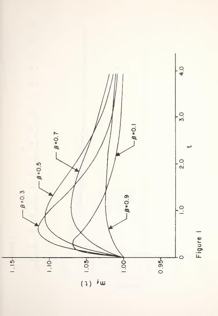
Figure 1. The intensity function m (t) for the EMA1 process. The functions
is plotted for values 3 = 0.1, 0.3, 0.5, 0.7 and 0.9 and A = 1. The
deviation from the constant, Poisson process value A = 1 is small. Unlike
the serial correlations for intervals this function does discriminate between
the cases 3 and 1-3.
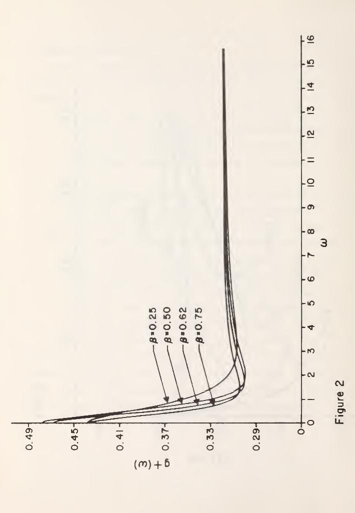
Figure 2. The spectrum of counts g,(w) for the EMA1 process. The spectrum
is flat with value 1/tt for the Poisson process (3=1 or 3 = 0). Unlike
the spectrum of intervals it does discriminate between the cases 3 and 1-6.
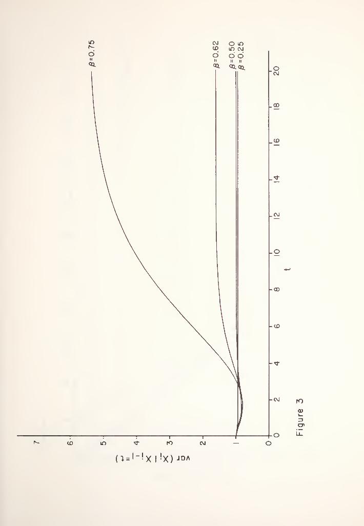
Figure 3. The conditional variance of X., given X = t, for the bivariate
exponential distribution (A = 1) arising in the EMA1 process.
Figure 4. The conditional variance of X , given X. _ = t, for the bivariate
exponential distribution (A = 1) arising in the EMA1 process.
Figure 5. The conditional correlation p~(t) for intervals X. , and X.,,,2 l-l i+I
given X. = t, for the EMA1 process. The joint distribution of X. . , X.,1 l-l i
X is a trivariate exponential distribution. Again there is differentiation
between the cases 3 and (1-3)
.
26
OFFICE OF NAVAI. KKSEARCHSTATISTICS AND PROBAIHLITY PROGRAM
BASIC DISTRIBUTION LISTFOR
UNCLASSIFIED TECHNICAL REPORTS
September 1974
CopiesStatistics and ProbabilityProgram
Office of Naval ResearchAttn: Dr. B.J. McDonaldArlington, Virginia 22217
Director, Naval ResearchLaboratory
Attn: Library, Code 2029(ON RIO
Washington, D. C. 20390
D f ense Documentation CenterCaieron StationAlexandria, Virjinia 22314
Defense Logistics StudiesIr.f ormation Exchange
Armv Logistics ManagementCenter
Attn: Arnold HixonFort Lee, Virginia 23801
Technical Information DivisionNaval Research LaboratoryWashington, D. C. 20390
Office of Naval ResearchNew York Area Office715 BroadwayAttn: Dr. Jack LadermanNew York, New York 10003
DirectorOffice of Naval ResearchBranch Office
^95 Summer StreetAttn: Dr. A. L. Powell.
Boston, Massachusetts 02210
DirectorOffice of Naval ResearchBranch Office
536 South Clark StreetAttn: Dr. A. R. DaweChicago, Illinois 60605
Office of Naval ResearchBranch Office
536 South Clark StreetAttn: Dr. P. PattonChicago, Illinois 60605
DirectorOffice of Naval ResearchBranch Office1030 East Green StreetAttn: Dr. A. R. LauferPasadena, California 91101
Office of Naval ResearchBranch Office
1030 East Green StreetAttn: Dr. Richard LauPasadena, California 91101
Office of Naval ResearchSan Francisco Area Office760 Market StreetSan Francisco, California
94102
Technical LibraryNaval Ordnance StationIndian Head, Maryland 20640
Dean of Research (Code 023)Naval Postgraduate SchoolMonterey, California 93940
Copies
Copies Copies
Nnval Ship Kng t nocring CenterPhi lade I pit la
Division Technical LibraryPhiladelphia, PA 19112 '
1
Bureau of Naval PersonnelDepartment of the NavyTechnical LibraryWashington, D.C. 20370 1
Library, Code 0212Naval Postgraduate SchoolMonterey, California 93940 1
LibraryNaval Electronics Laboratory
CenterSan Diego, California 92152 1
Naval Undersea CenterTechnical LibrarySan Diego, California 92132 1
Applied Mathematics LaboratoryNaval Ship Research andDevelopment Center
Attn: Mr. Gene H. GleissnerWashington, D.C. 20007 1
Office of Chief of NavalOperations (Op 964)
Pentagon, Room 4A538Washington, D.C. 20350 1
Naval Sea Systems Command(SEA 03F)
NC No. 3, Rm. 10S08Attn: Miss B.S. OrleansArlington, Virginia 20360 1
University of ChicagoDepartment of StatisticsAttn: Prof. P. MeierChicago, Illinois 60637 1
Stanford UniversityDepartment of Operations ResearchAttn: Prof. G. LiebermanStanford, California 94305 1
Florida State UniversityDepartment of StatisticsAttn: Prof. I.R. SavageTallahassee, Florida 32306 1
Florida State UniversityDepartment of StatisticsAttn: Prof. R.A. BradleyTallahassee, Florida 32306 1
Princeton UniversityDepartment of StatisticsAttn: Prof. J.W. TukeyPrinceton, New Jersey 08540 1
Princeton UniversityDepartment of StatisticsAttn: Prof. G.S. WatsonPrinceton, New Jersey 08540 1
Stanford UniversityDepartment of StatisticsAttn: Prof. T.W. AndersonStanford, California 94305 1
University of CaliforniaDepartment of StatisticsAttn: Prof. P.J. BickelBerkeley, California 94720 1
Harvard UniversityDepartment of StatisticsAttn: Prof. W.G. CochranCambridge, MA 02139 1
Columbia UniversityDepartment of Civil Engineeringand Engineering Mechanics
Attn: Prof. C. DermanNew York, New York 10027 1
Columbia UniversityDepartment of MathematicsAttn: Prof. H. RobbinsNew York, New York 10027 1
Library (Code 55)
Naval Postgraduate SchoolMonterey, California 93940 1
Copies Copies
New York UniversityInstitute of Mathematical
SciencesAttn: Prof. W.M. HirschNew York, New York 10453
University of North CarolinaDepartment of StatisticsAttn: Prof. W.L. SmithChapel Hill, North Carolina275U
University of North CarolinaDepartment of StatisticsAttn: Prof. M.R. LeadbetterChapel Hill, North Carolina
27514
University of California,San Diego
Department of MathematicsP.O. Box 109
Attn: Prof. M. RosenblattLa .Tolla, California 92038
University Tf WisconsinDepartment cf StatisticsAttn: Prof. G.E.P. BoxMadison, Wisconsin 53706
State University of New YorkChairman, Department of
StatisticsAttn: Prof. E. ParzenBuffalo, New York 14214
University of CaliforniaOperations Research CenterCollege of EngineeringAttn: Prof. R.E. BarlowBerkeley, California 94720
Yale UniversityDepartment of StatisticsAttn: Prof. F.J. AnscombeNew Haven, Connecticut 06520
1
Purdue UniversityDepartment of StatisticsAttn: Prof. S.S. GuptaLafayette, Indiana 47907 1
Cornell UniversityDepartment of Operations ResearchAttn: R.E. BechhoferIthaca, New York 14850 1
Stanford UniversityDepartment of MathematicsAttn: Prof. S. KarlinStanford, California 94305 1
Southern Methodist UniversityDepartment of StatisticsAttn: Prof. D.B. OwenDallas, Texas 75222 1
Daniel H. Wagner, AssociatesStation Square OnePaoli, Pennsylvania 19301 1
Stanford UniversityDepartment of Operations ResearchAttn: Prof. A.F. VeinottStanford, California 94305 1
Stanford UniversityDepartment of Operations ResearchAttn: Prof. D.L. IglehartStanford, California 94305 1
Stanford UniversityDepartment of StatisticsAttn: Prof. H. SolomonStanford, California 94305 1
University of North CarolinaDepartment of StatisticsAttn: Prof.. C.R. BakerChapel Hill, North Carolina 1
27514
University of WashingtonDepartment of MathematicsAttn: Prof. Z. W. BirnbaumSeattle, Washington 98105 1
Copies Copies
Clemson UniversityDepartment of Mathematical Sciences
Attn: Prof. K.T. Wal lenius
Clemson, South Carolina 29631 1
University of CaliforniaDepartment of StatisticsAttn: Charles E. AntoniakBerkeley, California 9A720 1
University of Southern CaliforniaElectrical Sciences DivisionAttn: Prof. W.C. LindseyLos Angeles, California 90007 1
Case Western Reserve UniversityDepartment of Mathematics and
StatisticsAttn: Prof. S. ZacksCleveland, Ohio 44106 1
Naval Research LaboratoryElectronics Division
(Code 5447)Attn: Mr. Walton BishopWashington, D.C. 20375 1
Commandant of the Marine Corps(Code AX)
Attn: Dr. A. L. SlafkoskyScientific Advisor
Washington, D. C. 20380 1
Program in LogisticsThe George Washington UniversityAttn: Dr. W.H. Marlow707 22nd Street, N.W.
Washington, D. C. 20037 1
Mississippi Test FacilityEast Resources Laboratory
(Code GA) 1
Attn: Mr. Sidney L. WhitleyBat St. Louis, Mississippi 39520
Naval Postgraduate SchoolDepartment of Operations Research
and Administrative SciencesAttn: Prof. P.A.W. LewisMonterey, California 93940 1
Southern Methodist UniversityDepartment of StatisticsAttn: Prof. W.R. SchucnnyDallas, Texas 75222 1
University of MissouriDepartment of StatisticsAttn: Prof. W. A. Thompson, Jr.
Columbia, Missouri 65201 1
Rice UniversityDepartment of Mathematical SciencesAttn: Prof. J.R. ThompsonHouston, Texas 77001 1
University of CaliforniaSystem Science DepartmentAttn: Frof. K. Yao 1
Los Angeles, California 90024
Naval Postgraduate SchoolDepartment of MathematicsAttn: Prof. P.C.C. WangMonterey, California 93940 1
University of CaliforniaDepartment of Information
and Computer ScienceAttn: Prof. E. MasryLa Jolla, California 92037 1
University of CaliforniaSchool of EngineeringAttn: Prof. N.J. BershadIrvine, California 92664 1
University of CaliforniaSchool of Engineering andApplied Science
Attn: Prof. I. RubinLos Angeles, California 90024 1
Virginia Polytechnic InstituteDepartment of StatisticsAttn: Prof. R. MyersBlacksburg, Virginia 24061 1
Copies Copies
University of MichiganDepartment of Industrial EngineeringAttn: Prof. R. L. Disney-
Ann Arbor, Michigan U810U 1
Naval Postgraduate SchoolDepartment of Operations Researchand Administrative Sciences
Attn: Prof. J.D. EsaryMonterey, California 939^0 1
Polytechnic Institute of New YorkDepartment of Electrical EngineeringAttn: Prof. M.L. ShoomanBrooklyn, New York 11201 1
Union CollegeInstitute of Industrial AdministrationAttn: Prof. L. A. AroianSchenectady, New York 12308 1
University o
Department c
St **t
* *~t * c~
Attn: Prof. W.J
New MexicoMathematics and
ZinnerAlbuquerque, New Mexico 8"106 1
Carnegie-Mellon UniversityDepartment of StatisticsAttn: Prof. J.E. KadcnePittsburgh, PA 15213 1
University of WyomincDepartment of StatisticsAttn: Prof. L.L. McDonaldLaramie, Wyoming 82070 1
Colorado State UniversityDerartment of ElectricalEngineering
Attn: Prof. L.L. Scharf, Jr.
Fort Collins, Colorado 80521 1
Virginia Polytechnic InstituteOffice Center for Public ChoiceDepartment of EconomicsAttn: Prof. M.J. HinichBlacksburg, Virginia 2Uo6l 1
Texas Tech UniversityCollege of EngineeringAttn: Prof. H.F. Martz, Jr.
Lubbock, Texas 79^09 1
Rockwell International CorporationRocketdyne DivisionAttn: Dr. N.R. Mann6633 Canoga Avenue 1
Canoga Park, California 9130U
Northwestern UniversityDepartment of Industrial Engineeringand Management Sciences
Attn: Prof. W.P. PierskallaEvanston, Illinois 60201 1
University of Southern CaliforniaGraduate School of BusinessAdministration and School ofBusiness
Attn: Prof. W.R. Blischke 1
Los Angeles, California 90007
National Security AgencyAttn: Dr. James R. MaarFort Meade, Maryland 20755 1
Naval Coastal Systems LaboratoryCode P76lAttn: Mr. CM. Bennett
Panama City, Florida 32^01 1
U.S. Army Research OfficeBox CM, Duke StationAttn: Dr. J. ChandraDurham, North Carolina 27706 1
National Security AgencyAttn: Mr. Glenn F. Stanly
Fort Meade, Maryland 20755 1
Naval Electronic Systems Command
(NELEX 320)
Attn: Mr. Richard RoyNational Center No. 1, Rm. 7W20
Arlington, Virginia 20360 1
Copies Copies
Mr. F. R. Del PrioriCode 22U
Operational Test and EvaluationForce (OPTEVFOR)
Norfolk, Virginia 23511 1
Southern Methodist University-
Computer Science/Operations ResearchCenter
ATTN: Prof. U.N. Bhat
Dallas, Texas 75275 1
University of FloridaDepartment of Industrial andSystems Engineering
ATTN: Prof. R.S. LeavenworthGainesville, Florida 32611 1
Massachusetts Institute ofTechnology
Department of MathematicsATTN: Prof. H. CnernoffCambridge, Massachusetts 02139 1
Dr. A. PetrasovitsRoom 207 B, Food & Drug BuildingTunney's PastureOttowa, Ontario K1A-0L2, CANADA 1
George Washington UniversityProgram in LogisticsATTN: Prof. N. Singpurvalla707 22nd Street, N.W.
Washington, D. C. 20037 1
Defence Communications AgencyDefense Communications EngineeringCenter
ATTN: Dr. M.J. Fischeri860 Wiehle AvenueReston, Virginia 22090 1
Advanced Research Projects Agency(ARPA) Research Center
Unit OneATTN: LCDR R. L. HimbargerMoffett Field, CA 8H035 1
Professor Ingram OlkinDepartment of StatisticsStanford UniversityStanford, California 94305 1
Professor J. NeymanDepartment of StatisticsUniversity of CaliforniaBerkeley, California 94720 1
Professor William HutchinasDepartment of MathematicsWhitman CollegeWalla Walla, Washington 99362 1
Professor Frank ProschanDepartment of StatisticsThe Florida State UniversityTallahassee, Florida 32306 1
Dr. Sam C. SaundersMathematics DepartmentWashington State UniversityPullman, Washington 99163 1
Dr. Seymour M. SeligOffice of Naval ResearchArlington, Virginia 22217 1
Professor Ernest M. ScheuerManagement Science Department:San Fernando State CollegeNorthridge, California 91324 1
Professor D. R. CoxImperial CollegeExhibition RoadLondon SW 7, England 1
Copies Copies
Professor Zvi ZeiglerIsrael Institute of TechnologyTechnionHaifa, Israel
Dr. Z. A. LomnickiThe Stone House, Oaken LanesOaken, CodsallStaffordshire, England
Professor Chin Long ChiangDivision of BiostatisticsUniversity of CaliforniaBerkeley, California 94720
Professor A. W. MarshallDepartment of StatisticsUniversity of RochesterRochester, New York
Professor Lucien Le CamDepartment of StatisticsUniversity o C *>_ 1lifornic
Berkeley, California 94720
Professor T. JayachandranCode 53JyNaval Postgraduate SchoolMonterey, California 93940
Dr. B. H. ColvinApplied Mathematics DivisionNational Bureau of StandardsWashington, D. C. 20234
Dr. Guil HollingsworthTechnical DirectorNaval Weapons CenterChina Lake, California 93555
Professor Nozer D. SingpurwallaOperations Research DepartmentGeorge Washington UniversityWashington, D. C. 20006
CDR A. L. Cicolani, SP1141Strategic Systems Project OfficeDepartment of the NavyWashington, D. C. 20390
Dr. Bill MitchellDepartment of Management SciencesCalifornia State UniversityHayward, California 94542 1
Mr. W. L. NicholsonStaff ScientistPacific Northwest laboratoriesBate lie BoulevardRichland, Washington 99352 1
LCDR W. J. HayneCOMSUBDEVCPUTWOSubmarine Base NLONGaston, Connecticut 06340 1
Mr. D. RubinsteinNational Institute of HealthBethesda, Maryland 20014 1
Professor Henry W. BlockDepartment of Operations Research
and StatisticsRensselaer Polytechnic InstituteTroy, New York 12181 1
Professor Janet MyhreClaremont Men's CollegeBauer Center, 900 Mills AvenueClaremont, California 91711 1
Professor Amrit L. GoelIndustrial Engineering and
Operations ResearchSyracuse UniversitySyracuse, New York 13210 1
Professor D.
Professor R.
Professor D.
Professor M.
Professor H.
Professor K.
Professor P.
Professor R.
CDR R. A. StephanProfessor J. D. EsaryDepartment of Operations Research
and Administrative SciencesNaval Postgraduate School
Monterey, California 93940
R. BarrW. ButterworthP. GaverB. KlineJ. LarsonT. MarshallR. MilchR. Read
1
1
1
1
1
1
1
1
1
10
Copies
Professor Peter BickelDepartment of StatisticsUniversity of CaliforniaBerkeley, California 94720 1
Professor E. J. WegmanStatistics DepartmentUniversity of North CarolinaChapel Hill, North Carolina 27514 1
Professor E. L. LehmanDepartment of StatisticsUniversity of CaliforniaBerkeley, California 94720 1
Professor E. ParzenComputing Science DepartmentSUNY (Buffalo)
4230 Ridge LeaAmherst, New York 14226 1
Professor D. P. Gaver 1
Professor A. Andrus 1
Professor D. A. Schrady 1
Code 55
Naval Postgraduate SchoolMonterey, California 93940