1

A Multi-agent Evolutionary Algorithm for Software

Module Clustering Problems

Jinhuang Huang, Jing Liu1

Key Laboratory of Intelligent Perception and Image Understanding of Ministry of Education,

Xidian University, Xi’an 710071, China

Xin Yao

Centre of Excellence for Research in Computational Intelligence and Applications (CERCIA),

School of Computer Science, The University of Birmingham, Birmingham B15 2TT, U.K.

Abstract: The aim of software module clustering problems (SMCPs) is to automatically find a good quality

clustering of software modules based on relationships among modules. In this paper, we propose a

multi-agent evolutionary algorithm to solve this problem, labeled as MAEA-SMCPs. With the intrinsic

properties of SMCPs in mind, three evolutionary operators are designed for agents to realize the purpose of

competition, cooperation and self-learning. In the experiments, practical problems are used to validate the

performance of MAEA-SMCPs. The results show that MAEA-SMCPs can find clusters with high quality

and small deviations. The comparison results also show that MAEA-SMCPs outperforms two existing

multi-objective algorithms, namely MCA and ECA, and two existing single-objective algorithms, namely

GGA and GNE, in terms of MQ.

Keywords: Software module clustering, multi-agent evolutionary algorithm, modularization quality.

1. Introduction

It is generally known that good modularization of software leads to systems that are easier

to design, develop, test, maintain, and evolve [1], [17]. However, it becomes difficult for large

software systems, especially they are not documented well [18], [24]. In general, a software

module clustering problem (SMCP) can be described as a problem to find a particular set of

modules, which is organized into clusters according to predefined criteria [2]. The problem of

finding the best clustering for a given set of modules is an NP hard problem [3]; that is, it is

1Corresponding author. For additional information regarding this paper, please contact Jing Liu, e-mail: neouma@163.com,

homepage: http://see.xidian.edu.cn/faculty/liujing/

2

impossible to exhaustively search for the best clustering but to estimate the goodness of a

cluster.

Mancoridis et al., who first suggested the search-based approach to module clustering [4],

formulates the attributes of a good modular decomposition as objectives, the evaluation of

which as a “fitness function” guides a search-based optimization algorithm. In this work, they

developed a tool called Bunch for automated software module clustering. Afterwards, guided

by the concept of search-based approaches, many heuristics methods have been proposed to

solve SMCPs, such as hill-climbing techniques, genetic algorithms and simulated annealing,

and so forth [3], [5], [6], [7], [10], [18], [19], [20], [21]. All these studies indicate that the

hill-climbing algorithm has performed the best in terms of both the solution quality and

execution time [8]. To guide the process of searching, an objective function is needed to

evaluate the objectives. In the software domain, the Modularization Quality (MQ) [30], which

is based on the trade-off between inter- and intra- connectivity, has been widely used as the

objective function.

Bunch includes a complete automated clustering engine and executes a set of

meta-heuristic clustering algorithms [30]. This approach partitions each level of subsystems

from the top level, the whole system is partitioned as subsystems at a high level. Finally, the

clustered system with the highest quality would be produced by the detailed level. It turns out

to be effective for large systems [3]. However, the shortcoming of hill-climbing methods is

premature convergence, which leads to local optima [6]. An attempt to overcome this problem

was a multiple hill-climbing approach ([6], [9]). Praditwong et al. [10] have proposed two

evolutionary algorithms, namely GGA and GNE, to solve SMCPs. They have obtained

comparatively good averaged MQ values, but they ignored the cohesion and coupling which

are significant measures of a software system. Praditwong et al. [11] also modeled the SMCP

as a multi-objective search problem and use evolutionary algorithms [25] to solve it, namely

MCA and ECA. MCA and ECA consider MQ, intra-edges and inter-edges as the objectives,

and obtained good results compared with other single-objective algorithms. Besides the MQ

measure, there are many other measures for SMCPs, such as EVM [31]. We choose MQ as

the primary measure in this paper as it is widely used for SMCPs.

In our previous work, a multi-agent genetic algorithm (MAGA) was proposed for

3

large-scale global numerical optimization [12]. MAGA integrated multi-agent systems with

GAs, and can optimize functions with 10000 dimensions, which is the first GA that can solve

functions with such high dimensions. It is also extended to solve constraint satisfaction

problems and combinatorial optimization problems successfully [13], [14]. Since MAGA

showed a good performance, we propose a multi-agent evolutionary algorithm to solve

SMCPs, labeled as MAEA-SMCPs.

With the intrinsic properties of SMCPs in mind, three evolutionary operators, namely the

neighborhood competition operator, the mutation operator and the self-learning operator are

designed. In MAEA-SMCPs, all agents live in a lattice-like environment. During the process

of interacting with the environment and the other agents, each agent increases energy (fitness)

as much as possible, so that MAEA-SMCPs can find the optima. In the experiments, a set of

problems extracted from real-world software with varying sizes are used to validate the

performance of MAEA-SMCPs. The experimental results show that MAEA-SMCPs has a

good performance, and outperforms other algorithms, such as GGA, GNE, MCA and ECA, in

terms of MQ.

The rest of this paper is organized as follows. Section 2 describes the SMCPs. Section 3

introduces the MAEA-SMCPs in detail. The experiments are given in Section 4. Finally, the

conclusions are given in Section 5.

2. Software Module Clustering Problems

Clustering provides the properties of groups instead of individuals within them [10].

Besides, clustering could not only reveal the internal relations and differences among data, but

also provide important basis for further analysis of data and discovery of knowledge. In

recently years, clustering methods have been widely used to assist analysis and

comprehension of software systems.

In an SMCP, a Module Dependency Graph (MDG) [4], which is a directed graph, has been

used as a representation of the problem. In MDGs, a vertex stands for a module (e.g.

Functions, sources files) in software system and a link, or an arc, stands for a relation (e.g.

Function calls) between two modules [26], [27], [28], [29]. The MDG file contains modules

4

and their relationships in the software system as a list of from-to-weighted information [6].

According to the characterization of edges, MDGs can be categorized into two types, the one

with and without weighted edges. If the edges of the MDG associate with positive number,

called weights, then the MDG is weighted; otherwise, it is unweighted.

Suppose an MDG is labeled as G = (V, E), where V={v1, v2, …, vn} is the set of n modules

and E is the set of links between modules. All modules need to be divided into k

non-overlapping clusters C1, C2, …, Ck; that is, C1∪C2∪...∪Ck=V, Ci≠∅ and Ci∩Cj=∅, i, j=1,

2, …, k, and i≠j. The purpose of SMCPs is to get clusters that are both densely intra-connected

and sparsely inter-connected.

There are two primitive principles of software design: coupling and cohesion. Coupling is a

measure of the degree to which clusters are related to other clusters, and cohesion denotes the

close relationship between components or modules within the same clusters [15], [21]. The

MDG partitioning, introduced above, tries to represent clusters of systems, which are

cohesive modules in the clusters and loosely connection between clusters [3].

Basic Modularization Quality (Basic MQ) was proposed in Bunch as a fitness function [3].

The Basic MQ is a metric which represents maximizing intra-edges and minimizing

inter-edges, where the intra-edge is a link between modules in the same cluster and the

inter-edge is a link between a module in a cluster and a module in another cluster. MQ is the

sum of the ratio of intra-edges and inter-edges in each cluster, called the Modularization

Factor (MFl) for cluster Cl. MFl can be defined as follows:

12

0, if 0

, if 0il

i j

iMF

i+

== > (1)

where i is the number of intra-edges and j is that of inter-edges for an unweighted problem [6].

For a weighted MDG, i and j are the sum of weights of intra-edges and inter-edges,

respectively.

The MQ can be calculated in terms of MF as

1

k

l

l

MQ MF=

=∑ (2)

The goal of MQ is to limit excessive coupling, but not to eliminate coupling altogether. It

implies that we should not simply pursue high cohesion and neglect proper coupling. Thus,

5

MQ attempts to make a trade-off between coupling (Inter-edges) and cohesion (Intra-edges)

through combining them into a single measurement. The aim is to reward increased cohesion

with a higher MQ score and to punish increased coupling with a lower MQ score [11].

3. Multi-agent Evolutionary Algorithm for SMCPs

3.1 Definition of software module clustering agents

Given an MDG with n modules, the arbitrary partition of this MDG can be represented as

character string coding X={x1, x2, ..., xn}, where xi is the cluster identifier of module i, which

can be represented by an integer number. As for the pair of modules i and j in X, if xi=xj,

modules i and j are in the same community; otherwise, they are in different ones. Thus, an

agent for SMCPs can be defined as follows:

Definition 1: An agent is a character string coding X={x1, x2, ..., xn} representing a

candidate partition for an MDG. Its energy is equal to the negative value of the following

objective function,

Energy(X) = - MQ(X) (3)

The purpose of X is to increase its energy as much as possible.

Definition 2: All agents live in a latticelike environment, L, which is called an agent lattice.

The size of L is Lsize×Lsize , where Lsize is an integer. Each agent is fixed on a lattice-point and

it can only interact with its neighbors. Suppose that the agent located at (i, j) is represented as

Li,j , i, j=1, 2, …, Lsize , then the neighbors of Li,j, Neighborsi,j are defined as follows:

{ }, , , , ,, , ,i j i j i j i j i jNeighbors L L L L′ ′ ′′ ′′= (4)

where 1 1

1size

i ii

L i

− ≠′ = =,

1 1

1size

j jj

L j

− ≠′ = =,

1

1

size

size

i i Li

i L

+ ≠′′ = =,

1

1

size

size

j j Lj

j L

+ ≠′′ = =.

For example, the agent lattice can be depicted as the one in Fig.1. Each circle stands for an

agent and any two connected agents can interact with each other. Besides, the data in each

circle means its position in the lattice.

6

Fig.1. The model of the agent lattice.

3.2 Evolutionary Operators for Agents

According to [12] [13], each agent has some behaviors. In addition to the aforementioned

behaviors of competition and cooperation, each agent can also increase its energy by using its

knowledge. On the basis of such behaviors, we design three evolutionary operators for agents.

The neighborhood competition crossover operator realizes the behavior of competition. The

mutation operator and the self-learning operator realize the behaviors of making use of

knowledge. Suppose that the three operators are performed on the agent located at (i, j), Li,j =

(l1, l2, …, ln ), and Maxi,j=(m1, m2,…, mn) is the agent with maximum energy among the

neighbors of Li,j, namely Maxi,j∈Neighborsi,j and ∀a∈Neighborsi,j, then

Energy(a)≤Energy(Maxi,j).

Neighborhood competition crossover operator: If Li,j satisfies (5), it is a winner; otherwise,

it is a loser.

Energy(Li,j)>Energy(Maxi,j) (5)

If Li,j is a winner, it can still live in the agent lattice. If Li,j is a loser, it must die, and its

lattice-point will be occupied by Maxi,j. The strategy we used to generate the agent to occupy

the lattice-point is the one-way crossover operator, which is introduced in [16]. In this

operator, the operation is conducted on Li,j and Maxi,j, Li,j is chosen as the source chromosome

while Maxi,j is the destination one. A node is first selected at random, and the cluster and

identifier of this node in Li,j is determined. Then, a value is assigned to all nodes belonging to

the same cluster in Maxi,j. In this way, information related to the community structure in A can

be transferred to Maxi,j. An example of the one-way crossover is given in Table 1, where node

7

3 is selected. The community label of node 3 is 2, which is also the community label of node

1. Then, the community label of node 1 in Maxi,j is changed to 2.

Table 1 An example for the one-way crossover with node 3 is selected.

V Li,j (source) Maxi,j (destination) Maxi,j (new)

1

2

3(selected)

4

5

2

1

2

3

1

1

3

2

5

3

2

3

2

5

3

*Bold values indicate changed positions

Mutation operator: In this operator, in order to make use of the information of one node

and its neighbors to which it links, a new mutation operator, namely neighbor-based mutation,

is designed, which works as follows: a node is selected randomly from Li,j , and then its

community label is changed to one of its neighbors.

Self-learning operator: According to our experiences, integrating local searches with EAs

can improve the performance for numerical optimization problems. There are several ways to

realize the local searches. Enlightened by MAGA [12], we propose the self-learning operator

which realizes the behavior of using knowledge by using a small scale MAEA regenerated

below. In order to be distinguished from the other parameters in MAEA, all symbols of the

parameters in this operator begin with an ‘s’.

In the self-learning operator, first, a new agent lattice, sL, with sLsize×sLsize agents, is

generated as follows: the best 10% agents in the current population are randomly put into this

lattice, and then other agents are initialized randomly. Second, the neighborhood competition

crossover operator and the mutation operator are iteratively performed on sL. Finally, the

agent with maximum energy found during the above process is returned. Algorithm 1

summarizes this operator in detail.

Algorithm 1: Self-learning operator

Input: sLk represents the agent lattice in the kth generation, and sL

k+1/2 is the mid-lattice between sL

k and

sLk+1

. sBestk is the best agent among sL

0, sL

1,…, sL

k, and sCBest

k is the best agent in sL

k. sPm is the

probability to perform the mutation operator, and sGen is the number of generations.

Output: Li,j.

1. begin

2. Randomly put best 10% agents in the current population to sL0, and then generate other agents in sL

0

randomly; update sBest0, and k←0;

8

3. Calculate energy of sL0, energy(sL

0)=MQ(sL

0);

4. Repeat

5. sLk+1/2

←NeighborhoodCompetition(sLk, sPc);

6. sLk+1

←NeighborMutation(sLk+1/2

, spm);

7. If Energy(sCBestk+1

)>Energy(sBestk),

8. sBestk+1

←sCBestk+1

;

9. else

10. sBestk+1

←sBestk, sCBest

k+1←sBest

k;

11. k←k+1

12. Until stop criteria (k>= sGen) are reached,

13. Li,j←sBestk.

14. end

3.3 Implementation of MAEA-SMCPs

In MAEA-SMCPs, the neighborhood competition operator is performed on each agent.

Consequently, the agents with low energy are cleaned out from the agent lattice so that there

is more developing space for the agents with high energy [12]. The mutation operator is

performed on each agent with probability Pm. The self-learning operator is performed on the

best 10% agents in each generation. Generally, the three operators employ different ways to

simulate the behaviors of agents and do performance to the results, respectively. Algorithm 2

summarizes MAEA-SMCPs in detail.

Algorithm 2: MAEA-SMCPs

Input: Lr represents the agent lattice in the rth generation, and L

r+1/2 is the mid-lattice between L

r and L

r+1.

Bestr is the best agent among L

0, L

1, …, L

r , and CBest

r is the best agent in L

r . Pc and Pm are the

probabilities to perform the neighborhood competition crossover operator and the mutation

operator, respectively.

Output: C={C1, C2, ..., Cn}: the partition with the best objective function value found.

1. begin

2. Initialization(L0), update Best

0, and r←0;

3. Calculate energy of L0, energy(L

0)=MQ(L

0);

4. repeat

5. Lr+1/2

←NeighborhoodCompetition(Lr, Pc);

6. Lr+1

←NeighborMutation(Lr+1/2

,pm);

7. Find the best 10% agents in Lr+1

, then perform the self-learning operator on them;

8. If Energy(CBestr+1

)>Energy(Bestr),

9. Bestr+1

←CBestr+1

;

10. else

11. Bestr+1

←Bestr, CBest

r+1←Best

r;

12. r←r+1

9

13. until stop criteria are reached

14. C←Bestr;

15. end

3.4 Computational complexity analysis

Here, we give a brief analysis on the computational complexity of MAEA-SMCPs. n and

m are used to denote the number of modules and the number of edges, respectively. To

calculate MQ, the main computational cost lies in calculating the number of inter-edges and

intra-edges. First, all modules are stored using an adjacency list, and the neighbor modules of

each module are stored in order. Then, assume that we have an array C[k], where k is the

number of clusters. Besides, For two connected modules u and v, where u belongs to cluster-i

and v belongs to cluster-j, C[i] plus one if i equals j; otherwise, C[i] plus one and C[j] plus one.

This process should be iterated for m times due to the number of edges of the system is m. In

order to calculate MQ, the array C should be traversed. Thus, the time complexity of

calculating MQ is O(m).

For MAEA-SMCPs, the main computational cost lies in Steps 3-12; the process of

searching for the best partition. The computational complexity of Step 4 is O(Lsize·Lsize·n), and

that of Step 5 is O(Lsize·Lsize·n2), where Lsize is the size of agent lattice L. For the calculation of

energy for each agent in Step 7, the computational complexity of Step 7 is O(Lsize·Lsize·m).

During the self-learning process, the worst case time complexity is

O(sLsize·sLsize·n)+O(sLsize·sLsize·n2)+O(sLsize·sLsize·m). Therefore, the worst case time

complexity for MAEA-SMCPs can be simplified as O(maxgen·Lsize·Lsize·(n2+ m)), where

maxgen is the number of iterations.

4. Experiments

In this section, 17 real-world problems [3], [6] are employed to validate the performance

of MAEA-SMCPs. The descriptions about these problems are given in Table 2. In the

following experiments, the parameters Pc, Pm, Lsize are set to 0.5, 0.05, 8, respectively.

Here, an experiment on a representative software system “mtunis” is first conducted as a

case study, and then the performance of the five algorithms optimizing MQ is compared on

the 17 problems.

10

Table 2

Descriptions of Testing Problems.

Name Description #Modules #Links

mtunis

ispell

rcs

bison

grappa

bunch

incl

icecast

gnupg

inn

bitchx

xntp

exim

mod_ss

ncurses

lynx

nmh

Turing operating system for educational purposes.

Spelling and typographical error correction software.

System used to manages multiple revisions of files.

Parser generator for converting grammar description int C.

Genome Rearrangements Analyzer.

Software Clustering tool(Essential java classes only).

Graph drawing tool.

Streaming MP3 audio codec media server.

Complete implementation of the OpenPGP standard.

Unix news group software.

Open source IRC client.

Time synchronization tool.

Message transfer agent for Unix systems.

Apache SSLITLS Interface.

Display and update software for text-only terminals.

Web browser for UNIX and VMS platforms.

Mail client software.

20

24

29

37

86

116

174

60

88

90

97

111

118

135

138

148

198

57

103

163

179

295

365

360

650

601

624

1653

729

1225

1095

682

1745

3262

4.1 Case study

Here, we first use the data “mtunis” (Mini-Tunis) [23], an operating system for education

purposes, as an example to explain the results in detail. Since “mtunis” is written in the Turing

language [22], each module stands for Turing modules and each edge stands for import

relationships between any two modules. Fig.4(a) shows the structure of “mtunis” as depicted

in the design documentation, which consists of 20 modules and 57 edges. Fig.4(b) shows the

obtained partitions by optimizing the basic MQ using MAEA-SMCPs.

In Fig.2(a), 6 different module clusters represent 6 major subsystems: red modules

constitute MAIN, sky blue modules constitute COMPUTER, dark blue and green modules

constitute FILESYSTEM (dark blue for FILE and green for INODE), pink modules constitute

DEVICE and yellow modules constitute GLOBALS.

Fig.2(b) is the automatically obtained partition for “mtunis” by optimizing the basic MQ

using MAEA-SMCPs. From Fig.2(b), we can see that the obtained partition is quite similar to

the partition in the design documentation. The main difference between Fig.2(a) and Fig.2(b)

lies in the confusion of FILE and INODE. For example, the module “Inode”, which belongs

to INODE, is divided falsely into FILE. What causes such misplacement is that the module

11

“Inode”, as an interface module, has a high connection with FILE. Similarly, the modules

“System” and “Panic”, which belong to GLOBAL (cluster with the yellow modules), are also

assigned falsely to other subsystems. The comparison between Fig.2(a) and Fig.2(b) shows

that the obtained partitions using MAEA-SMCPs still has space for improvement, although

they are quite similar.

(a) (b)

Fig.2. Two partitions of mtunis. (a) Structure of mtunis as depicted in the design

documentation; (b) obtained partition by optimizing the basic MQ using MAEA-SMCPs.

4.2 Results and discussions

Tables 3-6 report the averaged results of MAEA-SMCPs over 30 independent runs in terms

of MQ, intra-edges and inter-edges. Since GGA, GNE, MCA and ECA obtained good

performance, a comparison between MAEA-SMCPs and these four algorithms are also

conducted in Table 3-6. Among them, Table 4 reports the percentage that the new method

outperforms as per the results obtained.

As can be seen from Table 3 and 4, in terms of averaged MQ, MAEA-SMCPs outperforms

GGA and GNE on 6 out of 7 problems in unweighted problems. In weighted problems,

compared with GGA, besides the results for “inn”, “mod_ssl”, “ncurses”, the mean values of

MQ obtained by MAEA-SMCPs are better than those of GGA. However, MAEA-SMCPs

outperforms GNE in all weighted problems. Also, the standard deviations obtained by

MAEA-SMCPs are smaller than those of GGA and GNE in all problems, which indicates that

MAEA-SMCPs is more stable than GGA and GNE.

Compared with multi-objective problems, MAEA-SMCPs outperforms MCA and ECA in

most of the 17 problems in terms of MQ. Compared with MCA, the mean values of MQ

12

obtained by MAEA-SMCPs are better than those of MCA, and the standard deviations

obtained by MAEA-SMCPs are also smaller, which indicates that MAEA-SMCPs is more

stable than MCA. Meanwhile, compared with ECA, besides the results for “rcs”, “grappa”,

and “inn”, the mean values of MQ obtained by MAEA-SMCPs are also better than those of

ECA, and the standard deviations obtained by MAEA-SMCPs are also smaller, which

indicates that MAEA-SMCPs is also more stable than ECA.

Table 3

Comparison among 5 algorithms in terms of the averaged MQ.

Name MAEA-SMCPs GGA GNE MCA ECA

Mean ± STD Mean ± STD Mean ± STD Mean ± STD Mean ± STD

Not

weighted

mtunis

ispell

rcs

bison

grappa

bunch

Incl

2.314 ± 0.000

2.353 ± 0.000

2.228 ± 0.001

2.659 ± 0.001

12.495 ± 0.005

13.559 ± 0.024

13.569 ± 0.016

2.231 ± 0.051

2.338 ± 0.016

2.232 ± 0.029

2.231 ± 0.051

12.454 ± 0.144

12.938 ± 0.140

13.139 ± 0.170

2.289 ± 0.026

2.346 ± 0.014

2.263 ± 0.020

2.289 ± 0.026

10.828 ± 0.097

8.991 ± 0.100

8.143 ± 0.089

2.294 ± 0.013

2.269 ± 0.043

2.145 ± 0.034

2.416 ± 0.038

11.586 ± 0.106

12.145 ± 0.225

11.811 ± 0.351

2.314 ± 0.000

2.339 ± 0.022

2.239 ± 0.022

2.648 ± 0.029

12.578 ± 0.053

13.455 ± 0.088

13.511 ± 0.059

Weighted icecast

gnupg

inn

bitchx

xntp

exim

mod_ssl

ncurses

lynx

nmh

2.711 ± 0.000

7.004 ± 0.003

7.797 ± 0.002

4.307 ± 0.000

8.175 ± 0.004

6.440 ± 0.001

9.767 ± 0.003

11.410 ± 0.000

4.921 ± 0.003

8.973 ± 0.030

2.665 ± 0.042

6.874 ± 0.094

7.911 ± 0.037

4.252 ± 0.043

8.111 ± 0.083

6.251 ± 0.086

9.831 ± 0.072

11.452 ± 0.141

4.521 ± 0.073

8.770 ± 0.094

2.668 ± 0.016

6.072 ± 0.046

6.296 ± 0.057

3.565 ± 0.032

6.029 ± 0.065

4.848 ± 0.078

6.860±0.085

7.439±0.103

3.037 ± 0.031

4.576 ± 0.056

2.401 ± 0.057

6.259 ± 0.072

7.421 ± 0.077

3.572 ± 0.055

6.482 ± 0.110

5.316 ± 0.132

8.832 ± 0.097

10.211 ± 0.145

3.447 ± 0.086

6.671 ± 0.177

2.654 ± 0.039

6.905 ± 0.055

7.876 ± 0.046

4.267 ± 0.027

8.168 ± 0.076

6.361 ± 0.084

9.749 ± 0.071

11.297 ± 0.133

4.694 ± 0.060

8.592 ± 0.148

*Bold values indicate the best values among the five algorithms.

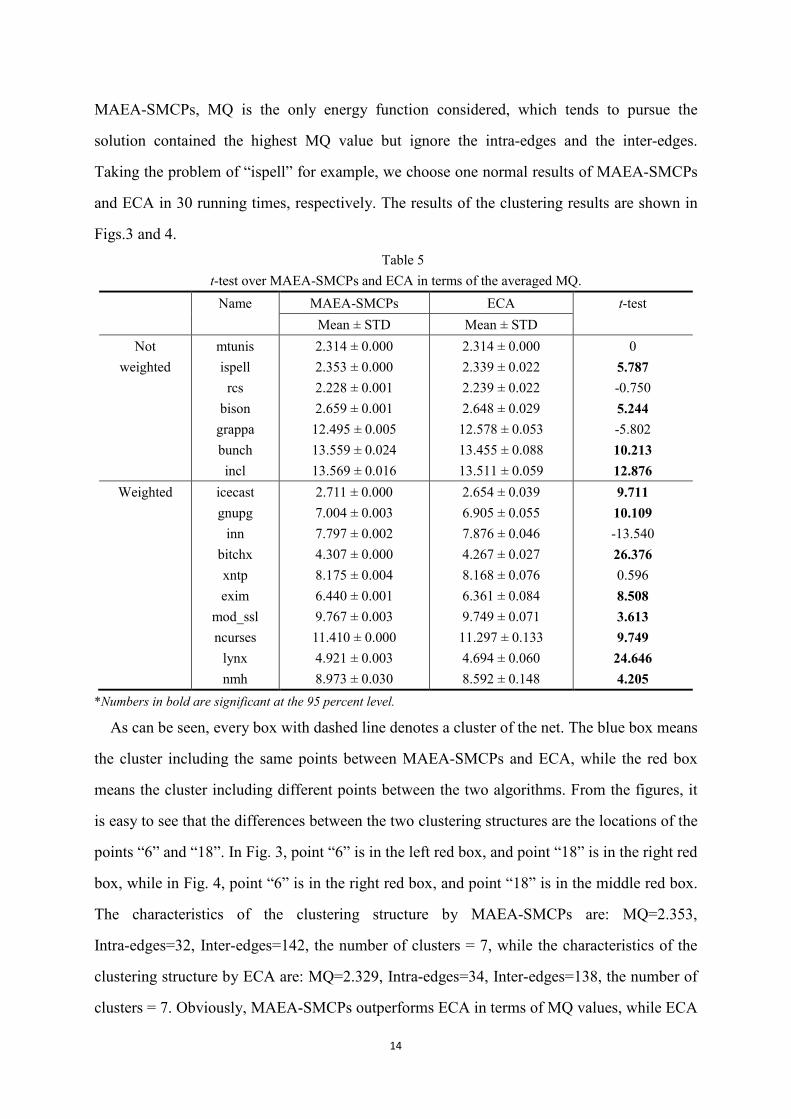
As can be seen from Table 3 and 4, the results of MAEA-SMCPs are similar to those of

ECA, so we try to analyze MAEA-SMCPs and ECA in terms of MQ using t-test in Table 5.

The results show that MAEA-SMCPs significantly outperforms ECA in 12 out of the 17

problems.

As we know, a better software system tends to have higher cohesion and lower coupling.

Cohesion is measured by the number of intra-edges in the modularization (those edges that lie

inside a cluster), while coupling is a measure of the number of inter-edges in the

modularization (the edges that connect two clusters) [11]. So we further compare intra-edges

13

and inter-edges between MAEA-SMCPs and two multi-objective algorithms (MCA and ECA)

in Table 6. As can be seen, the results provide strong evidence that MAEA-SMCPs

outperforms MCA for both unweighted and weighted graphs. That is, MAEA-SMCPs

outperforms MCA in all but 5 of the 17 problems studied. The comparison of MAEA-SMCPs

and ECA is somewhat inconclusive for unweighted graphs, with each approach able to

outperform the other in some cases. However, for weighted MDGs, the ECA approach

outperforms the MAEA-SMCPs in all cases but one of the 10 problems.

Table 4

Comparison between MAEA-SMCPs and GNE, MAEA-SMCPs and ECA in terms of the averaged MQ.

Name MAEA-SMCPs GNE ECA Percentage

(MAEA/GNE)

Percentage

(MAEA/ECA) Mean ± STD Mean ± STD Mean ± STD

Not

weighted

mtunis

ispell

rcs

bison

grappa

bunch

Incl

2.314 ± 0.000

2.353 ± 0.000

2.228 ± 0.001

2.659 ± 0.001

12.495 ± 0.005

13.559 ± 0.024

13.569 ± 0.016

2.289 ± 0.026

2.346 ± 0.014

2.263 ± 0.020

2.289 ± 0.026

10.828 ± 0.097

8.991 ± 0.100

8.143 ± 0.089

2.314 ± 0.000

2.339 ± 0.022

2.239 ± 0.022

2.648 ± 0.029

12.578 ± 0.053

13.455 ± 0.088

13.511 ± 0.059

1.118%

0.286%

-1.385%

1.385%

13.336%

32.327%

38.142%

0%

0.589%

-0.437%

0.418%

-0.626%

0.701%

0.491%

Weighted icecast

gnupg

inn

bitchx

xntp

exim

mod_ssl

ncurses

lynx

nmh

2.711 ± 0.000

7.004 ± 0.003

7.797 ± 0.002

4.307 ± 0.000

8.175 ± 0.004

6.440 ± 0.001

9.767 ± 0.003

11.410 ± 0.000

4.921 ± 0.003

8.973 ± 0.030

2.668 ± 0.016

6.072 ± 0.046

6.296 ± 0.057

3.565 ± 0.032

6.029 ± 0.065

4.848 ± 0.078

6.860±0.085

7.439±0.103

3.037 ± 0.031

4.576 ± 0.056

2.654 ± 0.039

6.905 ± 0.055

7.876 ± 0.046

4.267 ± 0.027

8.168 ± 0.076

6.361 ± 0.084

9.749 ± 0.071

11.297 ± 0.133

4.694 ± 0.060

8.592 ± 0.148

1.530%

13.618%

17.433%

16.717%

34.756%

24.904%

27.706%

35.547%

36.496%

48.256%

2.254%

0.103%

-1.132%

0.920%

0.008%

1.267%

0.239%

1.035%

4.283%

4.468%

According to [11], MCA and ECA are two multi-objective approaches, and each contains 5

objectives. In MCA, it chooses the sum of intra-edges of all clusters, the sum of inter-edges of

all clusters, the number of clusters, MQ, the number of isolated clusters as the 5 objectives

used to be optimized. However, ECA uses the difference between the maximum and

minimum number of modules in a cluster to take place of the fifth objective of MCA, the

number of isolated clusters. Compared to MCA, ECA prefers to choose the solutions which

have the less difference between the maximum and minimum number of modules in a cluster,

which accounts for the relatively homogeneous structures of the clustering. However, in

14

MAEA-SMCPs, MQ is the only energy function considered, which tends to pursue the

solution contained the highest MQ value but ignore the intra-edges and the inter-edges.

Taking the problem of “ispell” for example, we choose one normal results of MAEA-SMCPs

and ECA in 30 running times, respectively. The results of the clustering results are shown in

Figs.3 and 4.

Table 5

t-test over MAEA-SMCPs and ECA in terms of the averaged MQ.

Name MAEA-SMCPs ECA t-test

Mean ± STD Mean ± STD

Not

weighted

mtunis

ispell

rcs

bison

grappa

bunch

incl

2.314 ± 0.000

2.353 ± 0.000

2.228 ± 0.001

2.659 ± 0.001

12.495 ± 0.005

13.559 ± 0.024

13.569 ± 0.016

2.314 ± 0.000

2.339 ± 0.022

2.239 ± 0.022

2.648 ± 0.029

12.578 ± 0.053

13.455 ± 0.088

13.511 ± 0.059

0

5.787

-0.750

5.244

-5.802

10.213

12.876

Weighted icecast

gnupg

inn

bitchx

xntp

exim

mod_ssl

ncurses

lynx

nmh

2.711 ± 0.000

7.004 ± 0.003

7.797 ± 0.002

4.307 ± 0.000

8.175 ± 0.004

6.440 ± 0.001

9.767 ± 0.003

11.410 ± 0.000

4.921 ± 0.003

8.973 ± 0.030

2.654 ± 0.039

6.905 ± 0.055

7.876 ± 0.046

4.267 ± 0.027

8.168 ± 0.076

6.361 ± 0.084

9.749 ± 0.071

11.297 ± 0.133

4.694 ± 0.060

8.592 ± 0.148

9.711

10.109

-13.540

26.376

0.596

8.508

3.613

9.749

24.646

4.205

*Numbers in bold are significant at the 95 percent level.

As can be seen, every box with dashed line denotes a cluster of the net. The blue box means

the cluster including the same points between MAEA-SMCPs and ECA, while the red box

means the cluster including different points between the two algorithms. From the figures, it

is easy to see that the differences between the two clustering structures are the locations of the

points “6” and “18”. In Fig. 3, point “6” is in the left red box, and point “18” is in the right red

box, while in Fig. 4, point “6” is in the right red box, and point “18” is in the middle red box.

The characteristics of the clustering structure by MAEA-SMCPs are: MQ=2.353,

Intra-edges=32, Inter-edges=142, the number of clusters = 7, while the characteristics of the

clustering structure by ECA are: MQ=2.329, Intra-edges=34, Inter-edges=138, the number of

clusters = 7. Obviously, MAEA-SMCPs outperforms ECA in terms of MQ values, while ECA

15

beats MAEA-SMCPs in terms of intra-edges and inter-edges, which suggests that the ECA

approach tries to obtain the better MQ value with high intra-edges and low inter-edges, while

MAEA-SMCPs only considers the MQ value which may obtain the low intra-edges and the

high inter-edges. From the results of Table 6 we can see, although MAEA-SMCPs is a

single-objective approach, it outperforms MCA in most of the 17 problems, which indicates

that MAEA-SMCPs has a good capacity in dealing with the isolated clusters, and it has a

better optimizing ability than MCA does. Although MAEA-SMCPs is outperformed by ECA

in terms of intra-edges and inter-edges on some problems, its better MQ values indicates that

MAEA-SMCPs still has a potentiality to improve the optimizing results through the

optimization of the energy function.

Table 6

Comparison between MAEA-SMCPs and MCA, ECA in terms of Intra-edges and Inter-edges.

Name Intra-edges Inter-edges

MAEA-SMCPs MCA ECA MAEA-SMCPs MCA ECA

Mean ± STD Mean ± STD Mean ± STD Mean ± STD Mean ± STD Mean ± STD

mtunis

ispell

rcs

bison

grappa

bunch

Incl

27.000±0.000

32.000±0.000

41.233±0.142

45.200±0.223

99.400±0.300

101.433±0.333

141.667±1.649

24.633±2.092

23.100±3.220

45.133±15.335

40.367±8.231

84.767±11.190

73.567±8.324

91.767±14.024

27.000±0.000

30.033±2.798

47.567±7.859

52.800±6.217

101.167±8.301

111.700±5.305

140.200±3.836

60.000±0.000

142.000±0.000

243.533±0.285

267.600±0.446

391.200±0.600

525.133±0.667

436.667±3.298

64.733±4.185

159.800±6.440

235.733±30.669

277.267±16.463

420.467±22.380

580.867±16.648

536.467±28.048

60.000±0.000

145.933±5.595

230.867±15.719

252.400±12.434

387.667±16.601

504.600±10.611

439.600±7.673

icecast

gnupg

inn

bitchx

xntp

exim

mod_ssl

ncurses

lynx

nmh

1380.000±0.000

1242.133±1.133

1005.600±16.300

7469.000±0.000

1123.433±0.667

2847.167±0.969

2425.833±1.833

713.000±0.000

2885.500±0.025

2327.300±20.500

1609.900±294.921

1104.733±167.834

771.633±162.630

7644.633±2703.349

733.800±109.722

3279.300±563.781

2911.733±310.981

574.433±94.392

2428.567±863.007

2032.267±438.220

1643.167±208.189

1494.167±103.830

1336.900±190.263

7840.600±633.068

1117.967±54.502

3146.567±525.155

3476.800±244.174

806.367±57.515

3730.633±478.016

2704.600±236.782

8096.000±0.000

4916.667±2.267

5708.800±32.600

36290.000±0.000

3681.133±1.333

14759.667±1.938

14110.333±3.667

2794.000±0.000

22237.000±0.050

19331.400±41.000

7636.200±589.843

5192.530±335.669

6176.730±325.260

35938.700±5406.697

4460.400±219.445

12347.400±1127.563

12138.500±621.962

3071.130±188.785

23150.900±1726.014

19921.500±876.440

7569.670±416.378

4413.670±207.660

5046.200±380.526

35546.800±1266.136

3692.070±109.004

12612.900±1050.310

11008.400±488.348

2607.270±115.030

20546.700±956.032

18576.800±473.564

*Bold values indicate the best values among the three algorithms.

Tables 5-6 show that MAEA-SMCPs outperforms ECA on most problems in terms of the

averaged MQ, while ECA outperforms MAEA-SMCPs on most problems in terms of

intra-edges and inter-edges. Thus, we consider the location of solutions produced by

MAEA-SMCPs and ECA in Figs. 5-6, where intra-edges and MQ are chosen to see the

16

difference between them.

Fig.3. Clustering structure by MAEA-SMCPs Fig.4. Clustering structure by ECA

In Figs. 5 and 6, intra-edges and MQ are to be maximized, so the optimal solutions are

located in the uppermost and rightmost areas of the intra-edges and MQ space, while the least

optimal are located in the lowermost and leftmost area of the space. From the figures we can

see that each of two concentrates in a different region of the two objective search space. It is

apparent that MAEA-SMCPs focuses on the uppermost and leftmost areas of the space, while

ECA focuses on the lowermost and rightmost areas of the space in most problems. This

suggests that it is hard to say which algorithm is the better. Although the previous results

indicate that MAEA-SMCPs outperforms ECA in terms of MQ and ECA outperforms

MAEA-SMCPs in terms of intra-edges and inter-edges, the visualization of the result

locations in two-dimensional objective space indicates that each of the algorithms could not

produce the absolutely better results than the other one, but the solutions produced by

MAEA-SMCPs are more stable than ECA.

Next, we consider the location of solutions of MAEA-SMCPs and ECA in the intra-edges

and inter-edges space in Fig. 7. Finally, Table 7 reports the number of evaluations of the 3

algorithms (MAEA-SMCPs, MCA and ECA), which shows that the computational cost of

these 3 algorithm are similar.

17

24 25 26 27 28 29 301

1.5

2

2.5

3

3.5

Intra-edges

MQ

ECA

MAEA-SMCPs

27 28 29 30 31 32 33 34

2.24

2.26

2.28

2.3

2.32

2.34

2.36

2.38

2.4

2.42

2.44

Intra-edges

MQ

ECA

MAEA-SMCPs

(a) mtunis (b) ispell

30 35 40 45 50 55 60 652.16

2.18

2.2

2.22

2.24

2.26

2.28

2.3

Intra-edges

MQ

ECA

MAEA-SMCPs

35 40 45 50 55

2.62

2.64

2.66

2.68

2.7

2.72

2.74

Intra-edges

MQ

ECA

MAEA-SMCPs

(c) rcs (d) bison

85 90 95 100 105 110 115 12012.3

12.35

12.4

12.45

12.5

12.55

12.6

12.65

12.7

12.75

12.8

Intra-edges

MQ

ECA

MAEA-SMCPs

95 100 105 110 115 120 12513.25

13.3

13.35

13.4

13.45

13.5

13.55

13.6

13.65

13.7

Intra-edges

MQ

ECA

MAEA-SMCPs

(e) grappa (f) bunch

18

136 138 140 142 144 146

13.46

13.48

13.5

13.52

13.54

13.56

13.58

13.6

13.62

13.64

Intra-edges

MQ

ECA

MAEA-SMCPs

(g) incl

Fig.5. Solutions in the Intra-edges and MQ space for unweighted MDGs.

1200 1300 1400 1500 1600 1700 1800 1900 2000 2100

2.6

2.65

2.7

2.75

Intra-edges

MQ

ECA

MAEA-SMCPs

1150 1200 1250 1300 1350 1400 1450 1500 1550 1600 16506.75

6.8

6.85

6.9

6.95

7

7.05

7.1

Intra-edges

MQ

ECA

MAEA-SMCPs

(a) icecast (b) gnupg

900 1000 1100 1200 1300 1400 1500 16007.78

7.8

7.82

7.84

7.86

7.88

7.9

7.92

7.94

7.96

7.98

Intra-edges

MQ

ECA

MAEA-SMCPs

6500 7000 7500 8000 8500 90004.24

4.25

4.26

4.27

4.28

4.29

4.3

4.31

4.32

4.33

4.34

Intra-edges

MQ

ECA

MAEA-SMCPs

(c) inn (d) bitchx

19

1020 1040 1060 1080 1100 1120 1140 1160 1180 1200

8.12

8.14

8.16

8.18

8.2

8.22

8.24

Intra-edges

MQ

ECA

MAEA-SMCPs

2400 2600 2800 3000 3200 3400 3600 3800 4000

6.1

6.15

6.2

6.25

6.3

6.35

6.4

6.45

6.5

6.55

Intra-edges

MQ

ECA

MAEA-SMCPs

(e) xntp (f) exim

2200 2400 2600 2800 3000 3200 3400 3600 3800 4000

9.64

9.66

9.68

9.7

9.72

9.74

9.76

9.78

9.8

9.82

9.84

Intra-edges

MQ

ECA

MAEA-SMCPs

650 700 750 800 850 90011.15

11.2

11.25

11.3

11.35

11.4

11.45

11.5

11.55

Intra-edges

MQ

ECA

MAEA-SMCPs

(g) mod_ssl (h) ncurses

2800 3000 3200 3400 3600 3800 4000 4200 44004.5

4.55

4.6

4.65

4.7

4.75

4.8

4.85

4.9

4.95

5

Intra-edges

MQ

ECA

MAEA-SMCPs

1800 2000 2200 2400 2600 2800 3000 32008.3

8.4

8.5

8.6

8.7

8.8

8.9

9

9.1

9.2

9.3

Intra-edges

MQ

ECA

MAEA-SMCPs

(i) lynx (j) nmh

Fig.6. Solutions in the Intra-edges and MQ space for weighted MDGs.

20

28 29 30 31 32 33 34140

141

142

143

144

145

146

147

148

149

Intra-edges

Inte

r-ed

ges

ECA

MAEA-SMCPs

30 35 40 45 50 55 60200

210

220

230

240

250

260

270

Intra-edges

Inte

r-ed

ges

ECA

MAEA-SMCPs

(a) ispell (b) rcs

36 38 40 42 44 46 48 50 52 54 56245

250

255

260

265

270

275

280

285

290

Intra-edges

Inte

r-e

dg

es

ECA

MAEA-SMCPs

85 90 95 100 105 110 115 120350

360

370

380

390

400

410

420

Intra-edges

Inte

r-ed

ges

ECA

MAEA-SMCPs

(c) bison (d) grappa

Fig.7. Solutions in the Intra-edges and Inter-edges space for unweighted MDGs.

Table 7

Number of Evaluations of MAEA-SMCPs, ECA and MCA.

Name MAEA-SMCPs ECA/MCA

mtunis ispell

rcs bison

grappa bunch incl

icecast gnupg

inn bitchx xntp exim

mod_ssl ncurses

lynx nmh

300000 420000 550000

1180000 7850000

18320000 45580000 6830000

14780000 13550000 17560000 22440000 25450000 28540000 32560000 39890000 65430000

800000 1152000 1682000 2738000 14792000 26912000 60552000 7200000 15488000 16200000 18818000 24642000 27848000 36450000 38088000 43808000 78408000

5. Conclusions

In this paper, we propose a multi-agent evolutionary algorithm to solve SMCPs. The

experiments on practical problems illustrate the good performance of MAEA-SMCPs, and the

21

comparison also shows that MAEA-SMCPs outperforms two existing single-objective

algorithms and two existing multi-objective algorithms in terms of MQ. It could be further

studied through the optimization of the energy function, though the results of intra-edges and

inter-edges have great space to improve when compared with one of the multi-objective

algorithms, ECA. Meanwhile, the deviations obtained by MAEA-SMCPs are smaller than

those of existing algorithms, which implies that the performance of MAEA-SMCPs is more

stable. Besides, the number of evaluations of MAEA-SMCPs is less than that of other

algorithms, which further validates the effectiveness of MAEA-SMCPs. In this paper, we

only use MQ as the objective to solve SMCPs. Future research will focus on designing more

effective multi-objective algorithms for SMCPs.

Acknowledgments

This work is partially supported by the EU FP7-PEOPLE-2009-IRSES project under

Nature Inspired Computation and its Applications (NICaiA) (247619), the Outstanding

Young Scholar Program of National Natural Science Foundation of China (NSFC) under

Grant 61522311, the General Program of NSFC under Grant 61271301, the Overseas, Hong

Kong & Macao Scholars Collaborated Research Program of NSFC under Grant 61528205,

the Research Fund for the Doctoral Program of Higher Education of China under Grant

20130203110010, and the Fundamental Research Funds for the Central Universities under

Grant K5051202052.

References

[1] L. L. Constantine and E. Yourdon, Structured Design. Prentice Hall, 1979.

[2] K. Mahdavi, “A clustering genetic algorithm for software modularization with a multiple hill climbing

approach,” Ph.D. dissertation, Brunei University, U.K., 2005.

[3] B. S. Mitchell, “A heuristic search approach to solving the software clustering problem,” Ph.D.

dissertation, Drexel University, USA, 2002.

[4] S. Mancoridis, B. S. Mitchell, C. Rorres, Y. F. Chen, and E. R. Gansner, “Using automatic clustering

to produce high-level system organizations of source code,” Proc. Int’l Workshop Program

Comprehension, pp. 45-53, 1998.

[5] M. Harman, R. Hierons, and M. Proctor, “A new representation and crossover operator for

search-based optimization of software modularization,” Proc. Genetic and Evolutionary Computation

22

Conf., pp. 1351-1358, 2002.

[6] K. Mahdavi, M. Harman, and R. M. Hierons, “A multiple hill climbing approach to software module

clustering,” Proceedings of the International Conference on Software Maintenance, pp. 315-324,

2003.

[7] B. S. Mitchell and S. Mancoridis, “Using heuristic search techniques to extract design abstractions

from source code,” Proc. Genetic and Evolutionary Computation Conf., pp. 1375-1382, 2002.

[8] M. Harman, S. Swift, and K. Mahdavi, “An empirical study of the robustness of two module

clustering fitness functions,” Proceedings of the 2005 Conference on Genetic and Evolutionary

Computation, pp. 1029-1036, 2005.

[9] K. Mahdavi, M. Harman, and R. M. Hierons, “Finding building blocks for software clustering,” Proc.

of Genetic and Evolutionary Computation Conference, pp. 2513-2514, 2003.

[10] K. Praditwong, “Solving software module clustering problem by evolutionary algorithm,” Proc. of the

8th International Joint Conference Computer Science and Software Engineering, pp. 154-159, 2011.

[11] K. Praditwong, M. Harman, and X. Yao, “Software module clustering as a multi-objective search

problem,” IEEE Trans. Software Engineering, 37(2), pp. 264-282, 2011.

[12] W. Zhong, J. Liu, M. Xue, and L. Jiao, “A multiagent genetic algorithm for global numerical

optimization”, IEEE Trans. on Systems, Man, and Cybernetics, Part B, 34(2): 1128-1141, 2004.

[13] J. Liu, W. Zhong, and L. Jiao, “A multiagent evolutionary algorithm for constraint satisfaction

problems,” IEEE Trans. on Systems, Man, and Cybernetics, Part B, 36(1), 54-73, 2006.

[14] J. Liu, W. Zhong, and L. Jiao, “A multiagent evolutionary algorithm for combinatorial optimization

problems,” IEEE Trans. on Systems, Man, and Cybernetics Part B, 40(1), 229-240, 2010.

[15] R. S. Pressman, Software Engineering: A Practitioner's Approach, 6th ed., McGraw-Hill Higher

Education, 2005.

[16] M. Tasgin, A. Herdagdelen, and H. Bingol, “Community detection in complex networks using genetic

algorithms,” arXiv: 0711.0491, 2007.

[17] V. R. Basil, and A. J. Turner, “Iterative enhancement: A practical technique for software

development,” IEEE Trans. Software Engineering, vol. SE-1, no. 4, pp. 390-396, 1975.

[18] D. Doval, S. Mancoridis, and B. S. Mitchell, “Automatic clustering of software systems using a

genetic algorithm.” Proceedings of IEEE conference on Software Technology and Engineering

Practice (STEP'99), pp. 73-81, 1999.

[19] A. C. Kumari and K. Srinivas, “Software module clustering using a fast multi-objective

hyper-heuristic evolutionary algorithm,” International Journal of Applied Information Systems, vol. 5,

no. 6, pp. 12-18, 2013.

[20] A. C. Kumari, K. Srinivas, and M. P. Gupta, “Software module clustering using a hyper-heuristic

based multi-objective genetic algorithm,” Advance Computing Conference (IACC), 2013 IEEE 3rd

International, pp. 813-818, 2013.

[21] A. S. Mamaghani, and M. R. Meybodi, “Clustering of software systems using new hybrid algorithms.”

Proceedings of the Ninth IEEE International Conference on Computer and Information Technology

(CIT'09), vol. 1, 2009.

[22] R. C. Holt, and J. R. Cordy. The Turing Programming Language. Communications of the ACM, vol. 31,

no. 12, pp. 1410-1423, 1988.

[23] R. C. Holt. Concurrent Euclid, The UNIX System and Tunis. Addison Wesley, Reading, Massachusetts,

1983.

[24] S. D. Hester, D. L. Parnas, and D. F. Utter, “Using documentation as a software design medium.” Bell

23

System Technical Journal, vol. 60, no. 8, pp. 1941-1977, 1981.

[25] K. Praditwong and X. Yao, “A new multi-objective evolutionary optimisation algorithm: the

two-archive algorithm,” Proc. Int’l Conf. Computational Intelligence and Security, Y.-M. Cheung, Y.

Wang, and H. Liu, eds., vol. 1, pp. 286-291, 2006.

[26] S. C. Choi and W. Scacchi, “Extracting and restructuring the design of large systems,” IEEE Software,

vol. 7, no. 1, pp. 66-71, Jan. 1990.

[27] R. Lutz, “Recovering high-level structure of software systems using a minimum description length

principle,” Proc. 13th Irish Conf. Artificial Intelligence and Cognitive Science, Sept. 2002.

[28] D. H. Hutchens and V. R. Basili, “System structure analysis: clustering with data bindings,” IEEE

Trans. Software Engineering, vol. 11, no. 8, pp. 749-757, Aug. 1985.

[29] R. Koschke, “Atomic architectural component recovery for program understanding and evolution,”

PhD thesis, Inst. For Computer Science, Univ. of Stuttgart, 2000.

[30] S. Mancordis, B. S. Mitchell, Y. Chen, and E. R. Gansner, “Bunch: a clustering tool for the recovery

and maintenance of software system Structures”, in Proc. Of Int. Conf. of Software Maintenance, pp.

50-59, 1999.

[31] M. Harman, S. Swift, and K. Mahdavi, “An empirical study of the robustness of two module

clustering fitness functions”, in Proc. Of the 7th annual Conf. on Genetic and Evolutionary

Computation, pp. 1029-1036, 2005.