Page 1
Clemson UniversityTigerPrints
All Dissertations Dissertations
December 2016
A Multi-Model Approach to Design a RobustFixed-Order Controller to Improve Power SystemStabilityAbdlmnam Abdlrahem AbdlrahemClemson University, [email protected]
Follow this and additional works at: https://tigerprints.clemson.edu/all_dissertations
This Dissertation is brought to you for free and open access by the Dissertations at TigerPrints. It has been accepted for inclusion in All Dissertations byan authorized administrator of TigerPrints. For more information, please contact [email protected] .
Recommended CitationAbdlrahem, Abdlmnam Abdlrahem, "A Multi-Model Approach to Design a Robust Fixed-Order Controller to Improve Power SystemStability" (2016). All Dissertations. 2313.https://tigerprints.clemson.edu/all_dissertations/2313
Page 2
A MULTI-MODEL APPROACH TO DESIGN A ROBUST FIXED-
ORDER CONTROLLER TO IMPROVE POWER SYSTEM STABILITY
A Dissertation
Presented to
the Graduate School of
Clemson University
In Partial Fulfillment
of the Requirements for the Degree
Doctor of Philosophy
Electrical Engineering
by
Abdlmnam Abdlrahem
December 2016
Accepted by:
Richard E. Groff, Committee Chair
Taufiquar R. Khan
Randy Collins
Ramtain Hadidi
Page 3
II
ABSTRACT
The rapid increase in power system grid has resulted in additional challenges to
reliable power transfer between interconnected systems of a large power network. Large-
scale penetration of intermittent renewable energy increases uncertainty and variability in
power systems operation. For secure operation of power systems under conditions of
variability, it is imperative that power system damping controllers are robust.
Electromechanical oscillations in the range of 0.2 Hz to 1 Hz are categorized as inter-area
modes. These modes arise due primarily to the weak interconnections characterized by
long transmission lines between different operating areas of an interconnected power
system. One of the main challenges to secure operation of interconnected power systems
is the damping of these inter-area modes.
This dissertation introduces two multi-model approaches (loop shaping and 𝐻∞) to
designing a fixed-order robust supplementary damping controller to damp inter-area
oscillations. The designed fixed-order supplementary damping controller adjusts the
voltage reference set point of the Static Var Compensator (SVC). The two main
objectives of the controller design are damping low-frequency oscillations and enhancing
power system stability. The proposed approaches are based on the shaping of the open-
loop transfer function in the Nyquist diagram through minimizing the quadratic error
between the actual and the desired open-loop transfer functions in the frequency domain.
The 𝐻∞ constraints are linearized with the help of a desired open-loop transfer function.
This condition can be achieved by using convex optimization methods. Convexity of the
Page 4
III
problem formulation ensures global optimality. One of the advantages of the proposed
approach is the consideration of multi-model uncertainty. Also, in contrast to the methods
that have been studied in literature, the proposed approach deals with full-order model
(i.e., model reduction is not required) with lower controller order. In addition, most of the
current robust methods are heavily dependent on selecting some weighting filters: such
filters are not required in the loop-shaping approach. The proposed approaches are
compared with different existing techniques in order to design a robust controller based
on 𝐻∞ and H2 under pole placement. With large-scale power systems, it is difficult to
handle large number of states to obtain the system model. Thus, it becomes necessary to
use only input/output data measured from the system, and this data can be utilized to
construct the mathematical model of the plant. In this research, the mentioned approaches
are offered in order to design a robust controller based only on data by using system
identification techniques. The mentioned techniques are applied to the two-area four-
machines system and 68 bus system. The effectiveness and robustness of the proposed
method in damping inter-area oscillations are validated using case studies.
Page 5
IV
ACKNOWLEDGMENTS
First of all, I am thankful to God for giving me the strength to complete this dissertation.
I would like to express my sincere gratitude to my academic and research advisor, Dr.
Elham Makram, for her supervision and support in making this work possible.
I would also like to express my appreciation to Dr. Ramtain Hadidi and Dr. Alireza
Karimi for their support and valuable assistance during my research.
I also thank all the power group members for their help and research ideas, especially
Parimal Saraf, Karthikeyan Balasubramaniam and Hani Albalawy.
I would like to say thank you (I know that is not enough) to my beloved one who prays
every day and night for me to succeed in life: my Mother; even though you are far away,
your prayers are with me every minute. I want also to extend my deep appreciation to my
father, and my brothers and sisters for their prayers.
I owe my sincere gratefulness to my wife, who has been the main support during these
years. I want to extend my deep thankfulness to my children for their sweet smiles and
understanding.
Page 6
V
TABLE OF CONTENTS
Page
ABSTRACT ....................................................................................................................... ii
TABLE OF CONTENTS ................................................................................................. v
LIST OF FIGURES .......................................................................................................... x
LIST OF TABLES ......................................................................................................... xiii
LIST OF SYMBOLS ..................................................................................................... xiv
1 INTRODUCTION ..................................................................................................... 1
1.1 Motivation .............................................................................................................1
1.2 Literature Review ..................................................................................................5
1.3 Objective and Contributions .................................................................................8
1.4 Organization of the Dissertation .........................................................................11
2 POWER SYSTEM MODELING ........................................................................... 13
2.1 Synchronous Machine Model .............................................................................13
2.2 Excitation System ...............................................................................................16
2.3 Governor .............................................................................................................17
2.4 Power System Stabilizer (PSS) ...........................................................................18
2.5 Wind Energy Conversion Systems .....................................................................19
2.5.1 Wind turbine ................................................................................................20
Page 7
VI
Page
2.5.2 Doubly-fed induction generator ...................................................................21
2.6 Small Signal Stability ..........................................................................................24
2.6.1 Linearized state space model of a power system .........................................24
2.6.2 Power system oscillations ............................................................................29
2.6.3 Inter-area oscillations ...................................................................................30
2.7 Static VAR Compensator (SVC) ........................................................................30
3 𝑯∞ ROBUST CONTROLLER DESIGN ............................................................. 33
3.1 Class of models and controllers ..........................................................................34
3.2 𝑯∞ Robust Constraints .......................................................................................36
3.2.1 Uncertainty and Robustness Representation ...............................................36
3.2.2 Robust Stability and Performance ...............................................................36
3.3 The proposed approach .......................................................................................39
3.4 IEEE 68 Bus Test System and SVC Model ........................................................43
3.4.1 Test System ..................................................................................................43
3.4.2 Static Var Compensator ...............................................................................45
3.5 Controller Design Procedure ...............................................................................46
3.5.1 Selecting Inter-Area Modes .........................................................................46
3.5.2 Selecting Input/Output Signal ......................................................................47
Page 8
VII
Page
3.5.3 Choice of Operating Points ..........................................................................48
3.5.4 Desired Open-Loop Transfer Function (𝑳𝒅 )..............................................49
3.5.5 Weighting Filters (𝑾𝟏 and 𝑾𝟐) .................................................................51
3.5.6 Solving the Optimization Problem ..............................................................52
3.6 H2 Controller under Pole Placement ...................................................................52
3.7 Results and Discussion ........................................................................................54
3.7.1 Eigenvalue Analysis ....................................................................................55
3.7.2 Time Domain Analysis ................................................................................58
3.8 Time Delay ..........................................................................................................65
3.9 Conclusion ..........................................................................................................71
4 LOOP-SHAPING CONTROLLER ....................................................................... 72
4.1 Class of models and controllers ..........................................................................72
4.2 Robust Loop-Shaping Constraints ......................................................................73
4.3 Test Systems .......................................................................................................76
4.3.1 Two-Area Four-Machines Test System .......................................................77
4.3.2 16 Machines, 68 Bus System .......................................................................78
4.4 The Controller Design Procedure .......................................................................79
4.5 Frequency Response Analysis of the IEEE 68 Bus System ................................80
Page 9
VIII
Page
4.6 Simulation Results for the Two Case Studies .....................................................84
4.6.1 Time Domain Results for the Two-Area Test System .................................84
4.6.2 Two-Area System with different wind penetrations ....................................86
4.6.3 Eigenvalue Analysis ....................................................................................90
4.7 Time Domain Result for the 68 Bus System .......................................................91
4.7.1 𝑯∞ Controller .............................................................................................91
4.7.2 The proposed controller ................................................................................94
4.8 Conclusion ........................................................................................................102
5 DATA DRIVEN CONTROL ................................................................................ 104
5.1 Introduction .......................................................................................................104
5.2 Problem Formulation ........................................................................................106
5.2.1 Class of models and controller ..................................................................106
5.3 Robust controller Constraints ............................................................................109
5.4 Controller design steps ......................................................................................109
5.5 Test system ........................................................................................................113
5.6 Simulation Results ............................................................................................113
5.7 Conclusion ........................................................................................................119
6 CONCLUSION AND FUTURE WORK ............................................................. 120
Page 10
IX
Page
6.1 Conclusion ........................................................................................................120
6.2 Future Work ......................................................................................................123
References ...................................................................................................................... 124
APPENDIX: IEEE 68 Bus System Data ..................................................................... 134
Page 11
X
LIST OF FIGURES
Page
FIGURE 1.1 CLASSIFICATION OF POWER SYSTEM STABILITY ........................... 2
FIGURE 2.1 SYNCHRONOUS MACHINE SCHEMATIC ........................................... 14
FIGURE 2.2 SIMPLIFIED BLOCK DIAGRAM OF STANDARD EXCITATION
SYSTEM ................................................................................................................... 17
FIGURE 2.3 BLOCK DIAGRAM OF GOVERNOR SYSTEM ..................................... 17
FIGURE 2.4 A COMMON STRUCTURE OF PSS ......................................................... 18
FIGURE 2.5 SCHEMATIC OF A DFIG .......................................................................... 22
FIGURE 2.6 THE SVC CIRCUIT.................................................................................... 31
FIGURE 2.7 BLOCK DIAGRAM OF THE DYNAMIC MODEL OF AN SVC ........... 32
FIGURE 3.1 BLOCK DIAGRAM REPRESENTING AN UNCERTAIN FEEDBACK
SYSTEM ................................................................................................................... 36
FIGURE 3.2 NYQUIST PLOT......................................................................................... 37
FIGURE 3.3 LINEAR CONSTRAINTS ON NYQUIST PLOT...................................... 40
FIGURE 3.4 SINGLE LINE DIAGRAM OF THE 68 BUS TEST SYSTEM ................. 44
FIGURE 3.5 BLOCK DIAGRAM OF (A) SVC AND (B) CONTROL
REPRESENTATION ................................................................................................ 45
FIGURE 3.6 DAMPING RATIOS AND FREQUENCIES OF EIGENVALUES FOR
OP1, NORMAL OPERATING POINT .................................................................... 47
Page 12
XI
Page
FIGURE 3.7 CONTROLLABILITY INDICES OF CONTROLLABLE EIGENVALUES
BASED ON SELECTING THE LINE 42 TO 52 ...................................................... 48
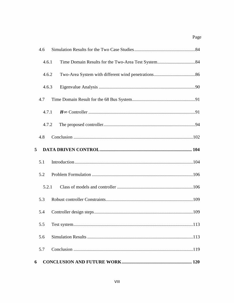
FIGURE 3.8 FREQUENCY RESPONSE OF THE THREE SELECTED PLANT
MODELS ................................................................................................................... 50
FIGURE 3.9 FREQUENCY RESPONSE OF THE WEIGHTING FILTERS................. 51
FIGURE 3.10 FREQUENCY RESPONSE OF THE ORIGINAL AND THE REDUCED
SYSTEM, OP1 .......................................................................................................... 54
FIGURE 3.11 MODES OF THE TEST SYSTEM UNDER THREE DIFFERENT
OPERATING POINTS.............................................................................................. 57
FIGURE 3.12 DYNAMIC RESPONSE OF THE SYSTEM UNDER THREE PHASE
FAULT AT BUS 8 (AREA 1) ................................................................................... 60
FIGURE 3.13 DYNAMIC RESPONSE OF THE SYSTEM UNDER THREE PHASE
FAULT AT BUS 49 (AREA 2) ................................................................................. 63
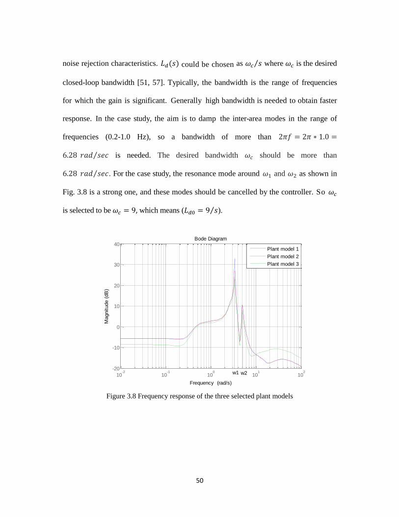
FIGURE 3.14 OUTPUT OF THE SVC AT DIFFERENT FAULT LOCATIONS,
OP 1 .......................................................................................................................... 64
FIGURE 3.15 BLOCK DIAGRAM OF OUTPUT SIGNAL TIME DELAY................ 651
FIGURE 3.16 DYNAMIC RESPONSE OF THE TEST SYSTEM WITH DIFFERENT
TIME DELAY ........................................................................................................... 68
FIGURE 3.17 DYNAMIC RESPONSE OF THE TEST SYSTEM WITH THE TWO
CONTROLLERS UNDER DIFFERENT TIME DELAY ........................................ 70
FIGURE 4.1 LOOP SHAPING IN NYQUIST PLOT...................................................... 76
Page 13
XII
Page
FIGURE 4.2 SINGLE LINE DIAGRAM OF TWO-AREA FOUR-MACHINES TEST
SYSTEM ................................................................................................................... 78
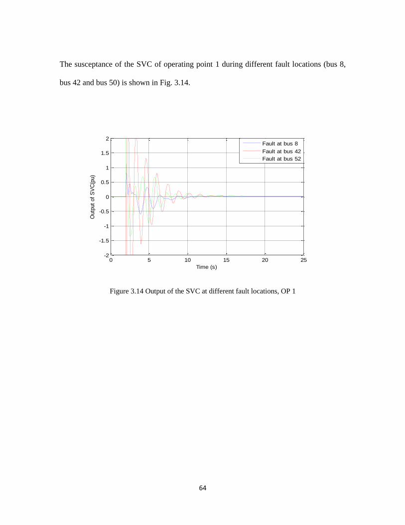
FIGURE 4.3 FREQUENCY RESPONSE OF THE THREE (A) MODELS, (B)
COMPLEMENTARY SENSITIVITY FUNCTIONS (C) SENSITIVITY
FUNCTIONS AND (D) OPEN LOOP TFS FOR THE 68 BUS SYSTEM CASE
STUDY ...................................................................................................................... 83
FIGURE 4.4 TIE-LINE POWER AND SPEED OF G1 AT DIFFERENT LOAD
CONDITIONS AND CHANGES IN SYSTEM TOPOLOGY. ................................ 89
FIGURE 4.5 FREQUENCY RESPONSE OF ORIGINAL SYSTEM, 12-, 7- AND 6-
ORDER REDUCED SYSTEM. ................................................................................ 93
FIGURE 4.6 TIE-LINE POWER AND ANGLE DIFFERENCE AT VARYING LOAD
CONDITIONS, FAULT LOCATIONS AND CHANGES IN SYSTEM
TOPOLOGY. ........................................................................................................... 101
FIGURE 5.1 SYSTEM REPRESENTATION ............................................................... 107
FIGURE 5.2 INPUT/OUTPUT IDENTIFICATION DATA ......................................... 111
FIGURE 5.3 MATCHING THE ORIGINAL MODEL WITH THE IDENTIFIED
MODEL ................................................................................................................... 113
FIGURE 5.4 DYNAMIC RESPONSE OF THE SYSTEM UNDER THREE PHASE
FAULT AT BUS 34 (AREA 2) ............................................................................... 116
FIGURE 5.5 DYNAMIC RESPONSE OF THE SYSTEM UNDER THREE PHASE
FAULT AT BUS 49 (AREA 2) ............................................................................... 118
Page 14
XIII
LIST OF TABLES
Page
TABLE 3.1 SVC PARAMETERS ................................................................................... 45
TABLE 3.2 EIGENVALUES, DAMPING RATIOS AND FREQUENCIES OF THE
INTER-AREA MODES OF THE TEST SYSTEM .................................................. 46
TABLE 3.3 DIFFERENT OPERATING POINTS FOR 68 BUS SYSTEM ................... 49
TABLE 3.4 DAMPING AND FREQUENCIES OF THE INTER-AREA MODES
UNDER DIFFERENT LOAD CONDITIONS OF THE 68 BUS SYSTEM ............ 56
TABLE 4.1 EIGENVALUE, DAMPING RATIO AND MODE FREQUENCY FOR
TWO-AREA SYSTEM ............................................................................................. 77
TABLE 4.2 EIGENVALUE, DAMPING RATIO AND MODE FREQUENCY FOR 68
BUS SYSTEM ........................................................................................................... 78
TABLE 4.3 DIFFERENT OPERATING POINTS FOR TWO-AREA TEST SYSTEM . 79
TABLE 4.4 DIFFERENT OPERATING POINTS FOR 68 BUS SYSTEM .................... 80
TABLE 4.5 DAMPING AND FREQUENCIES OF INTER-AREA MODES UNDER
DIFFERENT LOAD CONDITIONS ........................................................................ 90
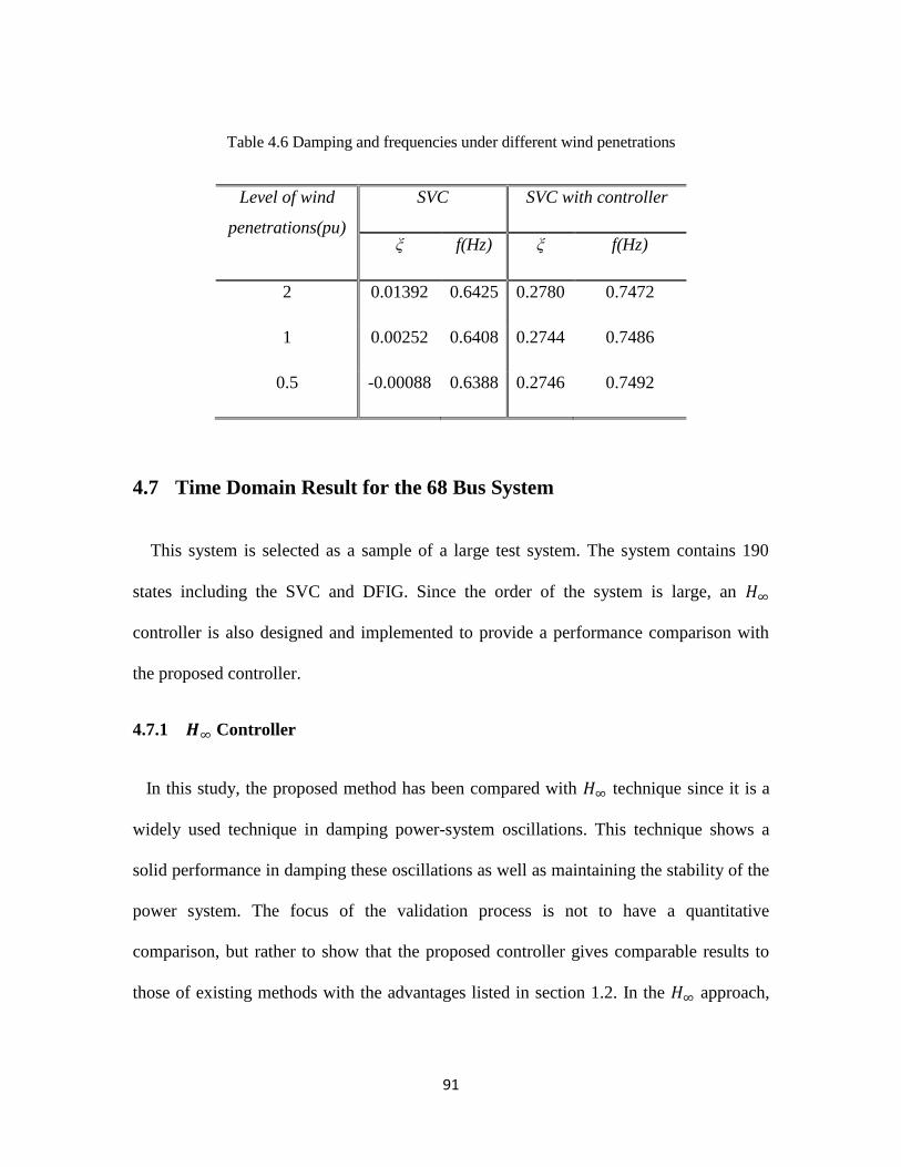
TABLE 4.6 DAMPING AND FREQUENCIES UNDER DIFFERENT WIND
PENETRATIONS ...................................................................................................... 91
TABLE 4.7 DAMPING AND FREQUENCIES OF THE INTER-AREA MODES
UNDER DIFFERENT LOAD CONDITIONS ........................................................ 102
Page 15
XIV
LIST OF SYMBOLS
x1 Leakage reactance
Ra Armature resistance
xd D-Axis synchronous reactance
x'd D-Axis transient reactance
x"d D-Axis sub-transient reactance
T'do Direct transient filed winding time constant
T"do Direct sub-transient filed winding time constant
xq Q-Axis synchronous reactance
x'q Q-Axis transient reactance
x"q Q-Axis sub-transient reactance
T'qo Quadrature transient filed winding time constant
T"qo Quadrature sub-transient filed winding time constant
H Inertia Constant
D Machine Damping
Page 16
XV
1/R Steady State Gain
Ta, Tb, Tc Exciter voltage regulator time constants
Efd,max, Efd,min Exciter max and min voltage regulator output
Kr Exciter constant
Eref Exciter reference voltage
Tr Exciter Time Constant
𝜔𝑟𝑒𝑓 Governor speed set point
Tmax Governor maximum Power Order On Generator Base
T1 Governor servo time constant
T2 HP turbine time constant
T3 Governor transient Gain Time Constant
T4 HP Section Time Constant
T5 Reheater Time Constant
Tn1
PSS lead Time Constant
Td1
PSS lag Time Constant
Tn2
PSS lead Time Constant
Td2
PSS lag Time Constant
Page 17
XVI
Ymax
PSS maximum Output Limit
Ymin
PSS minimum Output Limit
Tw PSS washout Time Constant
Kstab PSS gain
𝛿 Machine rotor Angle
𝜔 Generator angular speed
𝑒𝑞′ Transient quadrature axis voltage
𝑒𝑑′ Transient direct axis voltage
𝑒𝑞" Sub-transient quadrature axis voltage
𝑒𝑑" Sub-transient direct axis voltage
Efd Field voltage
AAT D-Axis Additional Leakage Time Constant
m Generator Input Mechanical Torque
e Generator Electromagnetic Torque
Page 18
1
CHAPTER ONE
1 INTRODUCTION
1.1 Motivation
Over the years, maintaining system stability has been a challenge to power engineers.
This problem can be categorized as power system modeling and correct assessment of
power system stability [1, 2]. A power system is modeled on algebraic and differential
equations. For large-scale power systems, these equations are more difficult to solve. To
achieve behavior similar to the real system, a detailed model has to be developed. Once a
mathematical model that is based on algebraic and differential equations is developed,
then the solution through numerical techniques is obtained.
Historically, solutions to the stability problem have been attempted since 1920. At that
time, computations of power systems were based on hand calculations. In 1950, analog
computers started to be used in power systems to simulate the transient stability problem.
In 1956, the first computer program on digital computers was created to make simulating
the transient stability problem easier.
Over the years, a high response of the excitation system was achieved to improve
transient stability. However, high response of the excitation system caused poor damping
in power system oscillations. The problem of poor damping has been coped with by using
power system stabilizers.
Page 19
2
A power system has never been in steady state condition all the time; disturbances may
occur at any time, and the challenge is to keep the system stable during these
disturbances.
Power system stability is the ability of a power system at specified operating conditions
to keep the system stable after being subjected to a disturbance, i.e. maintaining the
system variables, voltage and frequency within their limit [1]. The disturbance could be
large or small depending on the severity of the disturbance. Large disturbance includes
sizable change in generation, significant change in loads, line outages and the different
types of faults. Small disturbance is characterized by minimal changes in generation or
load.
Figure 1.1 Classification of power system stability
Page 20
3
Power system stability generally falls into three categories: rotor angle, voltage, and
frequency stability. Rotor angle, voltage and frequency stability have been classified as
large disturbance or small disturbance, short term or long term. These classifications are
shown in Figure 1.1.
The model of any system, no matter how detailed and complex, never represents the
real physical system. Normally, in conventional control design, uncertainty is
incorporated with the stability margin. The stability margin is a kind of safety factor: if
any changes occur (such as uncertainties and disturbances), they will not affect the
stability of the system, and the system will continue to behave in a satisfactory manner.
However, the uncertainties or perturbations are not quantified, nor has performance been
taken into account in terms of disturbance, noise, etc. The robust control method came to
the field to address these problems. The aim of the robust control is to achieve robust
performance and stability under a limit number of changes, uncertainties and
disturbances.
The power system is a nonlinear system, and it can be linearized around an operating
point. The nonlinearity and time-varying properties of the power system are modeled by
multi-model uncertainty and have been overcome by a robust design approach. In this
research, a fixed-order robust controller is designed based on different operating points,
which include the normal operating point as well as the worst operating point, to
overcome the uncertainties in the power system.
Power system grid has been increased rapidly, an achievement that has added more
challenges to reliable power transfer between interconnected systems of a large power
Page 21
4
network. Large-scale penetration of intermittent renewable energy increases uncertainty
and variability in power systems operation. For secure operation of power systems under
conditions of variability, it is imperative that power system damping controllers are
robust. Electromechanical oscillations in the range of 0.2 Hz to 1 Hz are categorized as
inter-area modes [1-5]. These modes arise due primarily to the weak interconnections
characterized by long transmission lines between different operating areas of an
interconnected power system. One of the main challenges in secure operation of
interconnected power systems is the damping of these inter-area modes. System stability
could be affected without adequate damping of these low-frequency oscillations [6].
Events such as the 1996 western interconnection blackout is an example.
Recently, Flexible AC Transmission System (FACTS) devices are being widely used
in power systems. The main purpose of these devices is to increase the capability of
transferred power between interconnected areas and to enhance the voltage profile as well
[3, 5, 7-26]. Static Var Compensator (SVC) is a shunt FACTS device that injects reactive
power to maintain the voltage at a point of connection in a certain range to enhance
system stability [27]. Controlling SVCs helps to damp inter-area oscillations. A
supplementary signal could be added to adjust the voltage reference set point of SVC to
achieve the desired damping [3, 19, 20, 24, 28, 29]. The location of SVCs for damping
inter-area oscillations is important; they are usually placed at either end of a tie-line.
Depending on system configuration, multiple SVCs might be required to improve the
overall system damping.
Page 22
5
1.2 Literature Review
Damping of inter-area oscillations in power systems using H2, 𝐻∞, 𝐻∞ loop-shaping,
and µ-synthesis methods has been previously studied [3, 10, 11, 24, 30-36]. The results
show that these methods of designing the controller have the ability to damp out inter-
area oscillations and enhance the stability of the power system. The solution to the 𝐻∞
control design problem is based on the Riccati equation approach. Generally, the
controller design based on this solution suffers from pole-zero cancellations between the
controller and the plant model. Recently, a linear matrix inequalities (LMIs) method has
been used to solve the 𝐻∞ control design problem [35-37]. The main concept of the 𝐻∞
loop-shaping method introduced is to augment the open-loop model by pre- and post-
compensators to get the desired shape. Then the controller is designed by solving the 𝐻∞
optimization problem [38].
Most of these designs are based on nominal operating point, i.e. the control objectives
from H2 and 𝐻∞ formulations are guaranteed an operating point [39]. On some occasions,
the system might not be operating close to a nominal operating point, and the controller
might not work as expected. The order of the controller is considered a key factor, since
the controller is implemented in computers and devices that have limited memory and
computing power. Implementing a high-order controller both in hardware and software is
a challenging task and leads to numerical problems. Even though there are some methods
to reduce the order of the controller, they do not guarantee that the reduced controller will
achieve the requirements of stability and performance.
Page 23
6
New techniques are presented in [10, 11] for designing a robust controller for multi-
modal uncertainty using H2 and 𝐻∞ under pole placement; however, these techniques
require reducing the order of the plant model. Also, the designed controller based on
these techniques leads to high-order controller, compared with the proposed approach.
Recently, Wide Area Measurements (WAMs) have been used to design the controller
[2, 4, 14, 15, 23, 40-42]. Phasor Measurements Units (PMUs) are installed in specific
locations to monitor and control modern power systems and improve their stability and
security [43-49]. Inter-area oscillations could be damped out using wide area
measurements. Good results have been achieved by applying WAMs to the damping
controller as shown in [14, 23].
The main challenge of using WAMs to design a robust controller to damp the inter-
area oscillations is the issue of the signal transmission delay [43, 46, 48]. The signal
provided to the controller from PMUs has some delay in communications channels, and
this delay may affect the performance of the controller. In [48], a summary of
communication delays is shown among six PMUs installed in different locations at
Jiangsu, China. The summary shows that the PMU signal could be delayed in the range
(7 to 81 ms). Also, the latency of PMU data of the QUEBEC power system is listed in
[50], which shows the total estimated latency (109 ms).
Large interconnected power systems have thousands of generators, and it is not
possible to model each generator in detail. For example, to model one single generator, a
simple generator can be modeled as a 3rd-order model. The 6th-order model of a
synchronous machine gives enough information by having a complete detailed model.
Page 24
7
Each generator has a turbine model, governor model, exciter model, and automatic
voltage regulator model. Each of these models has a different number of state variables
that will correspond to the number of state variables of the machine. So, as a whole, one
generator has to be modeled by at least 12 to 13 states, and if the system has a huge
number of generators, the number of the state variables will be very high. Thus it
becomes quite difficult to handle this number of states to obtain the system model. Most
of the control approaches in literature used to damp inter-area oscillations are based on
plant models (parametric models). In such situations, input/output data measured from
the plant can be used to construct the mathematical model of the plant. This approach is
called data driven and can be achieved by using system identification techniques. In this
approach, the knowledge of the plant is not required. PMUs can be used to provide
input/output data to the control center.
To summarize, the challenges of the existing approaches are:
1- The power system is known as a high-order system. These approaches are based
on reducing the order of the plant model (system). The model reduction is the
process of reducing the order of a given system to the extent that the response of
the reduced system is similar to that of the full-order system. Hence, there is loss
of information. The level of loss of information is dependent on the order to
which the system is reduced and the method used. On the other hand, the
proposed method does not require any model order reduction. In addition, model
Page 25
8
order reduction is an O(n^3) operation. Hence, computing model order reduction
for large systems is computationally expensive.
2- The order of the controller based on existing approaches is comparatively high for
large systems with the proposed approach, since it is the sum of the orders of the
reduced plant model plus the order of the weighting filters as mentioned in [2].
For example, in reference [14] the order of the controller is 10 and it is 7 in
reference [10].
3- Most of the existing designs are based on the nominal operating point, i.e. the
control objectives from H2 and 𝐻∞ formulations are guaranteed an operating
point. However, a power system is a non-stationary system wherein operating
points change for every dispatch at the system operator level. Hence, performance
of such controllers degrades depending on the deviation between current
operating point and the nominal operating point for which the controller was
designed.
4- In literature most of the control approaches that were used to damp inter-area
oscillations are based on parametric models.
1.3 Objective and Contributions
The contribution of this research is introducing a new technique to design a fixed-order
linearly parameterized controller using the 𝐻∞ approach. The main idea of the proposed
approach is based on the shaping of the open-loop transfer function under an infinite
Page 26
9
number of convex constraints on the Nyquist diagram. The control objective is to reduce
the distance between the designed open-loop transfer function and the desired one by
minimizing their quadratic error in the frequency. The desired transfer function needs to
be specified in order to carry out the optimization and design of the controller. The
proposed technique can handle both stable and unstable plant models. In this work,
however, only stable plant models are considered. Frequency Domain Robust Control
(FDRC) Toolbox, which is introduced in [51], is used in this research to design the
fixed-order robust controller in both approaches. This technique doesn’t suffer from other
methods’ drawbacks.
Thus, the contributions of the dissertation are as outlined below:
The proposed techniques do not need model order reduction. The controller
design techniques presented in this research can be used in full-order systems
for designing a robust 𝐻∞ controller, since the order of the controller is fixed,
without sacrificing the computational time required (which is taken care of by
convexifying the problem). Therefore, the need for using an approximate
reduced order model is eliminated. The proposed approaches can also use a
reduced order system.
The resulting controller order is less than that of other existing methods. For
example, the IEEE 68 bus test system used in this research has 190 states, and
it is considered a large system. To design a robust controller using conventional
methods, the system has to be reduced, and the order of the controller is equal
to the order of the reduced system. The IEEE 68 bus system (190 states) is
Page 27
10
reduced to 7 states. Thus, the order of the controller using, for example 𝐻∞,
will be the order of the reduced system 7 plus the order of the weighting filters.
On the other hand, only the 4th-order controller is designed based on the
proposed approach for the same system, and it demonstrates very good results.
The designed controller is fixed order, which means that the user can specify
the order of the controller; it does not depend on the order of the system.
Multi-model uncertainty is considered, which means that the robustness is
guaranteed in a wide range of changing the operating point. The controller can
be designed based on different operating points to overcome the uncertainty of
the power system.
The issue of time delay of feedback signals has been addressed using a multi-
model optimization approach.
Convex formulation guarantees a global optimal solution while minimizing the
norm between open-loop transfer function and desired transfer function.
The designed controller has been integrated into the Power System Toolbox
(PST). The results are verified by matching the Eigenvalues of the test systems
after adding the controller in both the FDRC Toolbox and the PST.
In chapter five, a fixed-order robust controller has been designed based only on
frequency-domain data (obtained using spectral analysis of measured I/O data);
no parametric model is required.
Page 28
11
1.4 Organization of the Dissertation
The dissertation is divided into six chapters as follows:
Chapter one: gives an introduction and definition of power system stability and also
describes the issue of inter-area oscillations. Research review related to the topic of this
dissertation is summarized in this chapter. The challenges of the existing approaches as
well as the contributions of this research are also mentioned in this chapter.
Chapter two: describes the dynamic model of the components of power systems,
including synchronous machine, excitation system, governor, and power system
stabilizer. The dynamic equations of wind turbine are also explained in this chapter.
Introduction to small signal stability and linearization of the power system around an
equilibrium point are discussed.
Chapter three: the loop-shaping approach based on shaping the open-loop transfer
function on the Nyquist diagram through minimizing the distance between the actual and
the desired open-loop transfer function is introduced in this chapter. The controller design
procedure is explained in detail. The proposed approach is applied to the two-area four-
machines system and the IEEE 68 bus system. The effectiveness and robustness of the
proposed method in damping inter-area oscillations are validated through case studies.
Chapter four: introduces the 𝐻∞ approach to designing a robust fixed-order controller.
The proposed 𝐻∞ approach is based on shaping the closed-loop sensitivity functions in
the Nyquist diagram through constraints on their infinity norm. The 𝐻∞ constraints are
Page 29
12
linearized with the help of a desired open-loop transfer function. In this chapter, a multi-
model optimization method is used to include the effect of time delay. The IEEE 68 bus
system is cited to verify the designed controller under different operating conditions.
Chapter five: the method explained in chapter three is extended to design a robust
controller based on input/output data using system identification techniques. In this
approach, the knowledge of the plant is not required. Phasor measurement units (PMUs)
can be used to provide input/output data to the control center.
Chapter six: summarizes results, conclusions, and future work.
Page 30
13
CHAPTER TWO
2 POWER SYSTEM MODELING
In this chapter, the dynamic model of power system components is explained. The
power system contains different dynamic components that are used to maintain system
stability. These components need to be modeled in order to find the nonlinear dynamic
model of the power system. The dynamic model of these devices can be modeled by
several algebraic and differential equations as explained in the following sections [1, 2].
2.1 Synchronous Machine Model
Synchronous generators are the main source of electric energy in power systems. The
stability of a power system is defined as the ability of interconnected synchronous
generators in different areas to maintain synchronism after the system becomes subjected
to a disturbance. Basically, system stability depends on different factors that determine
the severity of the disturbance: the initial operating condition, and the nature and size of
the disturbance. Consequently, it becomes important to understand the modeling and
dynamic behavior of the synchronous generators. The synchronous generator equations
describe the dynamic behavior of synchronous machines. There are different types of
models for synchronous machines, and the order of the model depends upon the purpose
of study [1].
Page 31
14
Figure 2.1 Synchronous machine schematic
The 6th-order model of a synchronous machine provides enough information by having a
complete detailed model. In this dissertation, a 6th-order model of a synchronous
machine, as described herein, has been used.
The dynamic equations of the 6th-order synchronous machine model that is used in this
thesis are given below in (2.1) – (2.6).
�̇� = 𝛺𝑏(𝜔 − 𝜔𝑠) (2.1)
�̇� =1
2𝐻(𝑇𝑚 − 𝑇𝑒 − 𝐷(𝜔 − 𝜔𝑠)) (2.2)
θ
Reference axis
Direct axis
Quadrature axis
a
a’
b’
b
c’
c
q’
q
f
d
d’
f’
ω Direction of rotation
Page 32
15
qe =1
𝑇′𝑑0
(−𝑒′𝑞 − (𝑥𝑑 − 𝑥′
𝑑 − 𝛾𝑑)𝑖𝑑 + (1 −𝑇𝐴𝐴
𝑇′𝑑0
) 𝐸𝑓𝑑) (2.3)
de =1
𝑇′𝑞0
(−𝑒′𝑑 − (𝑥𝑞 − 𝑥′
𝑞 − 𝛾𝑞)𝑖𝑞) (2.4)
)E)((1
fd'
00 d
AAddddqq
d
qT
Tixxee
Te
(2.5)
))((1
0
qqqqdd
d
d ixxeeT
e
(2.6)
where d and q are given as follows:
)( ),(0
0
q
0
0qq
q
q
q
q
dd
d
d
d
dd xx
x
x
T
Txx
x
x
T
T
(2.7)
The solution of power flow reveals the initial values of active and reactive power as well
as the voltage and the angle ( ,,, VQP gg ) of the system. The power system variables are
related to the machine equations by the equations given in (2.7) – (2.9)
𝐼 =𝑃𝑔 + 𝑖 ∗ 𝑄𝑔
𝑉 (2.8)
𝛿 = ∠(𝑉 + (𝑟𝑎 + 𝑖 ∗ 𝑥𝑞)𝐼) (2.9)
𝑣𝑑 = 𝑉𝑠𝑖𝑛(𝛿 − 𝜃)
𝑣𝑞 = 𝑉𝑐𝑜𝑠(𝛿 − 𝜃) (2.10)
Page 33
16
2.2 Excitation System
The main purpose of an excitation system is to provide a direct current to the field
winding of a synchronous machine. An excitation system provides two essential
functions: control and protection, to satisfy the power system performance. The control
function includes controlling voltage and reactive power flow to enhance power system
stability. The protective functions of the excitation system are responsible for monitoring
the limits of the synchronous machine and the other equipment to avoid exceeding their
limit. Generally there are three different types of excitation system: DC, AC, and static
excitation systems [52]. A basic block diagram of the standard excitation system is
shown in Fig.2.2.
The excitation system can b represented by the following dynamic equations (2.11) to
(2.13):
�̇�𝑟 =1
𝑇𝑟
(𝐾𝑟𝐸 − 𝐸𝑟) (2.11)
�̇�𝑎 =1
𝑇𝑏((1 −
𝑇𝑐
𝑇𝑏) (𝐸𝑟𝑒𝑓 − 𝐸𝑟) − 𝐸𝑎) (2.12)
where 𝐸𝑎 is an internal state of the lead-lag compensator.
�̇�𝑓𝑑 =1
𝑇𝑎(𝐾𝑎𝐸𝑎 − 𝐸𝑓𝑑) (2.13)
The value of 𝐸𝑓𝑑 is used in the machine equations
Page 34
17
r
r
sT
K
1 b
c
sT
sT
1
1
a
a
sT
K
1
ErefEfd,max
Efd,min
EfdEt
EaEr
Figure 2.2 Simplified block diagram of standard excitation system
2.3 Governor
The main function of the governor is to control the output power of a synchronous
machine as the power system changes. The speed of the synchronous machine accelerates
or de-accelerates depending on the change in loads. The governor increases the speed of
the synchronous machine by increasing the input of real power until the frequency settles
at the synchronous speed. The governor control action is relatively slow compared with
other controllers, so the time constants associated with the governor are small. The block
diagram of the governor dynamic model is shown in Fig 2.3 [2].
R
1
11
1
sT 2
3
1
1
sT
sT
PrefPmax
Pmin
Pmech
ref
4
5
1
1
sT
sT
Figure 2.3 Block diagram of governor system
The dynamic equations that represent the governor model have been listed in (2.14) –
(2.16).
Page 35
18
�̇�𝑔1 =1
𝑇1(𝑃𝑖𝑛 − 𝑥𝑔1) (2.14)
�̇�𝑔2 =1
𝑇2((1 −
𝑇3
𝑇2) 𝑥𝑔1 − 𝑥𝑔2) (2.15)
�̇�𝑔3 =1
𝑇4((1 −
𝑇5
𝑇4) (𝑥𝑔2 +
𝑇3
𝑇2𝑥𝑔1) − 𝑥𝑔3) (2.16)
2.4 Power System Stabilizer (PSS)
The power system stabilizer is normally installed in the system to damp out the local
power system oscillations. PSS is very useful for improving the dynamic stability of the
power system. It helps the damping of these oscillations by adding a supplementary
damping signal to the reference of the excitation circuit. PSS has three main blocks: gain,
phase compensation, and washout circuit or reset block. Fig 2.4 shows the simple block
diagram of PSS.
stabKw
w
sT
sT
1 2
1
1
1
sT
sT
Vssmax
Vssmin
Vss
4
3
1
1
sT
sT
x 1̇ x 2̇
Figure 2.4 A common structure of PSS
The dynamic equations related to the PSS are given in (2.17) – (2.19).
Page 36
19
�̇�1 =1
𝑇𝑤
(−𝐾𝑠𝑡𝑎𝑏∆𝜔 + 𝑥1) (2.17)
�̇�2 =1
𝑇2((1 −
𝑇3
𝑇2) (𝐾𝑠𝑡𝑎𝑏∆𝜔 + 𝑥1) − 𝑥2) (2.18)
�̇�𝑠𝑠 =1
𝑇4((1 −
𝑇5
𝑇4) (𝑥2 + (
𝑇3
𝑇2
(𝐾𝑠𝑡𝑎𝑏∆𝜔 + 𝑥1))) − 𝑉𝑠𝑠) (2.19)
2.5 Wind Energy Conversion Systems
Due to an ever increasing penetration of renewable energy sources in the power grid,
it has become essential to study the impact of these sources on the dynamics and stability
of the system. A Wind Energy Conversion System (WECS) essentially comprises a wind
turbine, a generator and power electronic controls. An important assumption for
modeling WECS in fundamental frequency simulations is that the power electronic
converters are represented as current sources. This is a routine methodology used for
modeling of power electronic components in power system dynamic studies. One more
important assumption in this work is that multiple wind generators are aggregated into a
single machine for the purpose of dynamic analysis [53].
Page 37
20
2.5.1 Wind turbine
The wind turbine extracts the kinetic energy from the wind and converts it into
mechanical energy that in turn rotates the rotor of the wind generator and generates
electricity. The mechanical power output of the turbine shaft is given as:
𝑃𝑚 =𝑛𝑔𝑒𝑛
2𝜌𝑎𝑖𝑟𝐴𝑏𝑙𝑎𝑑𝑒𝐶𝑝(𝛽, 𝜆)𝑣3
𝑤 (2.20)
Tip-speed ratio, 𝜆 =𝑅𝑏𝑙𝑎𝑑𝑒𝜔𝑚
𝑣𝑤
where 𝑛𝑔𝑒𝑛 is the number of wind generators, 𝜌𝑎𝑖𝑟 is the density of air, 𝐴𝑏𝑙𝑎𝑑𝑒 is the area
of the blades swept by the rotor [m2], 𝑣𝑤 is the wind speed [m/s], 𝛽 is called the pitch
angle, 𝜔𝑚 is the angular speed of the blades, and bladeR is the radius of the rotor blades.
Pitch angle control is necessary to protect the blades from damage when the wind speeds
are very high. It curtails the amount of power extracted from wind by pitching the blades
of the turbine. 𝐶𝑝(𝛽, 𝜆) is called the ‘coefficient of performance,’ and it is a function of
the tip-speed ratio and the pitch angle. The ),( pC curve is approximated as given in
(2.21) using (2.22) [54].
𝐶𝑝 = 0.22 (116
𝜆𝑖− 0.4𝛽 − 5) 𝑒
−12.5𝜆𝑖 (2.21)
1
𝜆𝑖=
1
𝜆 + 0.08𝛽−
0.035
𝛽3 + 1 (2.22)
The dynamic equation representing pitch angle control is given in (2.23).
Page 38
21
𝛽 =(𝐾𝑝𝜑(𝜔𝑚 − 𝜔𝑟𝑒𝑓) − 𝛽)
𝑇𝑝 (2.23)̇
where 𝜑 is a function that allows changing the pitch angle only when the difference
(𝜔𝑚 − 𝜔𝑟𝑒𝑓) is above a certain threshold. Since pitch angle control only operates in
super-synchronous speeds (speed greater than synchronous speed), an anti-windup limiter
sets 𝛽 to zero for sub-synchronous speeds.
The electromechanical equation associated with the shaft of the turbine is given in (2.24).
�̇�𝑚 =𝑇𝑚−𝑇𝑒
2𝐻𝑚 (2.24)
where 𝜔𝑚 is the rotor speed, 𝑇𝑚 is the mechanical torque, 𝑇𝑒 is the electrical torque and
𝐻𝑚 is the inertia of the rotor.
2.5.2 Doubly-fed induction generator
The most commonly used type of generator for wind power generation is a Doubly-
Fed Induction Generator (DFIG). A grid connected to a DFIG involves a wound rotor
induction machine and has terminals on both stator and rotor. However, with an induction
machine, the rotor frequency is dependent on the operating slip of the machine. So, an
AC/DC/AC converter is used to connect the rotor terminals to the grid. The AC/DC/AC
converter enables variable speed operation and also enables the control of output real and
reactive power. The machine stator and rotor voltages in terms of machine currents and
rotor speed m are given in (2.25) – (2.28) [55]. A schematic diagram of DFIG is shown
Page 39
22
in Fig. 2.5. The bidirectional arrows signify that the power can flow in either direction
depending on the mode of operation (sub-synchronous or super-synchronous).
Figure 2.5 Schematic of a DFIG
𝑣𝑑𝑠 = −𝑟𝑠𝑖𝑑𝑠 −𝑑𝜆𝑑𝑠
𝑑𝑡+ 𝜆𝑞𝑠 (2.25)
𝑣𝑞𝑠 = −𝑟𝑠𝑖𝑞𝑠 −𝑑𝜆𝑞𝑠
𝑑𝑡+ 𝜆𝑞𝑠 (2.26)
𝑣𝑑𝑟 = −𝑟𝑟𝑖𝑑𝑟 −𝑑𝜆𝑑𝑟
𝑑𝑡+ (1 − 𝜔𝑚)𝜆𝑞𝑟 (2.27)
𝑣𝑞𝑟 = −𝑟𝑟𝑖𝑞𝑟 −𝑑𝜆𝑞𝑟
𝑑𝑡+ (1 − 𝜔𝑚)𝜆𝑑𝑟 (2.28)
where 𝑖𝑑𝑠, 𝑖𝑞𝑠, 𝑖𝑑𝑟 , 𝑖𝑞𝑟 are the direct and quadrature axis stator and rotor currents,
𝑣𝑑𝑠 , 𝑣𝑞𝑠, 𝑣𝑑𝑟 , 𝑣𝑞𝑟 are the direct and quadrature axis stator and rotor voltages,
𝜆𝑞𝑠, 𝜆𝑞𝑟 , 𝜆𝑑𝑠, 𝜆𝑠𝑟 are the stator and rotor direct and quadrature axis fluxes, 𝑟𝑠 and 𝑟𝑟 are
Page 40
23
stator and rotor resistances. It has to be noted that the equations (2.25) – (2.28) are shown
per unit.
The DFIG is represented as a constant power load for the purpose of dynamic simulation.
This choice influences the update of bus voltages (algebraic variables) during dynamic
simulations. For representing DFIG in dynamic studies, the transients associated with
stator and rotor flux have been neglected. It is normal to neglect stator flux transients
(even in synchronous machines) in fundamental frequency simulations since they are
very fast to die out. The rotor flux transients are neglected because the current control
loops of the voltage source converters counteract them. Therefore, the differential terms
in equations (2.25) – (2.28) are set to zero. The electrical torque output of the machine in
terms of stator and rotor currents is given in (2.29) [56].
𝜏𝑒 = 𝑥𝑚(𝑖𝑞𝑟𝑖𝑑𝑠 − 𝑖𝑑𝑟𝑖𝑞𝑠) (2.29)
where mx is the magnetizing reactance.
As mentioned previously, the dynamics associated with the voltage source converters
(VSC) are quite fast, and thus the converter can be modeled as an ideal current source.
The rotor direct and quadrature currents 𝑖𝑑𝑟 and 𝑖𝑞𝑟 form the state variables. The current
𝑖𝑑𝑟 is used to control the bus voltage (in other words reactive power injection), whereas
𝑖𝑞𝑟 is used for controlling the rotor speed. The dynamic equations associated with the
VSC are given in (2.30) and (2.31).
Page 41
24
𝑖̇𝑞𝑟 =
((−𝑥𝑠 + 𝑥𝑚
𝑥𝑚𝑣𝑏𝑢𝑠)
𝑃𝑚(𝜔𝑚)𝜔𝑚
𝑖𝑞𝑟)
𝑇𝜖 (2.30)
𝑖̇𝑑𝑟 = 𝐾𝑣(𝑣𝑏𝑢𝑠 − 𝑣𝑟𝑒𝑓) −𝑣𝑏𝑢𝑠
𝑥𝑚− 𝑖𝑑𝑟 (3.31)
where 𝑥𝑠 is the stator reactance, 𝑣𝑏𝑢𝑠 is the voltage of the bus where the DFIG is
connected, 𝐾𝑣 is the voltage control gain, 𝑃𝑚(𝜔𝑚) is the power extracted from the wind
as a function of the rotor speed, and 𝑇𝜖 is the power control time constant. Since, 𝑖̇𝑞𝑟 and
𝑖̇𝑑𝑟 cannot exceed certain physical limits, anti-windup limiters are used.
2.6 Small Signal Stability
Small signal stability is defined as the ability of the power system to maintain
synchronism under small perturbations [1]. Small perturbations may occur in any part of
the power system due to the daily changes in loads and generations. The first step in
studying the small signal stability of any power system is to linearize it around an
operating point since small disturbance is considered a small change in the system. Thus,
a linear model can be made around this operating condition. The effect of small signal
stability can be studied by applying small disturbances on the resulting model.
Furthermore, there are different types of control theories that have been used to design a
controller based on a linear model.
2.6.1 Linearized state space model of a power system
A large-scale power system consists of a large number of machines and each machine
has its own controller. The components of a power system are represented by Differential
Page 42
25
and Algebraic Equations (DAE), and some of the differential equations are nonlinear.
Consequently, the first step in performing small signal analysis is to linearize the
dynamic model of the interconnected power system. The set of differential and algebraic
equations that represent the power system can be listed as given in (2.32a-c) [1, 2].
�̇� = 𝑓(𝑥, 𝑥𝑎, 𝑢) (2.32𝑎)
0 = 𝑔(𝑥, 𝑥𝑎, 𝑢) (2.32𝑏)
𝑦 = ℎ(𝑥, 𝑥𝑎, 𝑢) (2.32𝑐)
where 𝑥 and 𝑥𝑎 are the vectors of state and algebraic variables respectively, u and y
represent the variables of input and output vectors, equation (2.32a) represents the power
system dynamics. The power flow equation is described in (2.32b). Equation (2.32c)
describes output in terms of state and input variables.
In small signal stability, the dynamic behavior of a power system is linearized around an
equilibrium point where 0x . Then, the system can be analyzed around this point. The
state space matrices (A, B, C and D) can be obtained based on the linearized model of the
power system around the equilibrium point. The equilibrium point of a power system is
obtained from the power flow results.
Two approaches exist that can determine state space matrices:
1) Using analytic Jacobian.
2) Using numerical differentiation for approximating the Jacobian.
Page 43
26
In this work, the power system toolbox (PST) software package based on MATLAB is
used. PST employs the second approach to obtain the state space matrices. The
differential and algebraic equations are solved in PST successively. The modified Euler’s
method, which is also known as the predictor and corrector method, is used to calculate
and update the state and algebraic variables. This approach has two steps: the first one
applies a small change to the variables ( x and u ) and the changes are (∆𝑥 𝑎𝑛𝑑 ∆𝑢). In
the second step, the change in the nonlinear function f in equation (2.32a) are (𝜕𝑓
𝜕𝑥) and
(𝜕𝑓
𝜕𝑢), which produces the matrices A and B. A similar approach is used to calculate matrix
C. In the transfer function that represents the power system components, the order of the
numerator is less than or equal to the order of the denominator, so the D matrix is
composed of zeros. Thus, the power system can be represented by the state space form as
given in (2.33).
�̇� = 𝐴𝑥 + 𝐵𝑢
𝑦 = 𝐶𝑥 (2.33)
For small disturbance resulting in small change in ((∆𝑥 𝑎𝑛𝑑 ∆𝑢), the system equations
can be written in a linearized form as given in (2.34).
∆�̇� = 𝐴∆𝑥 + 𝐵∆𝑢
∆𝑦 = 𝐶∆𝑥 (2.34)
Page 44
27
where
𝐴 = [𝜕𝑓
𝜕𝑥], 𝐵 = [
𝜕𝑓
𝜕𝑢] and C= [
𝜕𝑔
𝜕𝑥]
Note that A is the state matrix, B is the input matrix and C is the output matrix.
The matrix A provides important information about the system behavior. It can be shown
that the closed loop poles of the system represented by these matrices are the roots of the
characteristic equation:
𝑑𝑒𝑡(𝐴 − 𝜆𝐼) = 0 (2.35)
These roots are called Eigenvalues 𝜆(𝜆 = 𝜆1, 𝜆2, … . . , 𝜆𝑛) of the state matrix A.
Eigenvalues are very important in analyzing power system dynamics; they indicate how
much the system is close to or far from the stability limit. Eigenvalues can be obtained by
solving equation (2.35). By looking at the Eigenvalues 𝜆𝑖 = 𝛼𝑖−+𝑗𝜔𝑖 , in which numbers
can be real or complex, a full picture of small signal stability can be gained.
Properties of Eigenvalues
1- The system is said to be stable if all the real parts of the Eigenvalues have a
negative sign (𝛼𝑖).
2- The system is said to be unstable if all the real parts of the Eigenvalues have a
positive sign.
Page 45
28
3- The system becomes marginally stable if all the real parts of the Eigenvalues have
a negative sign except one that has only an imaginary part ( 𝑗𝜔−+ ), and the system
in this case will be in oscillatory mode.
There are two important parameters for analyzing the small signal stability of the
oscillatory mode: its damping (𝜉𝑖) and frequency (𝑓𝑖), which can be given as:
𝜉𝑖 =−𝛼𝑖
√𝛼𝑖2 + 𝜔𝑖
2
(2.36)
𝑓𝑖 =𝜔𝑖
2𝜋
Two Eigenvectors—“Right Eigenvector (REV) and Left Eigenvector (LEV)” —are
associated with each Eigenvalue, as described in equation (2.37).
𝐴Ф𝑖 = 𝜆𝑖Ф𝑖
Ѱ𝑖𝐴 = 𝜆𝑖Ѱ𝑖 (2.37)
where Ф𝑖 and Ѱ𝑖 are the vectors of the right and left Eigenvectors respectively as shown
below:
Ф𝑖 = [Ф1 Ф2 … … . Ф𝑛]
Ѱ𝑖 = [Ѱ1 Ѱ2 … … . Ѱ𝑛]𝑇
Ф and Ѱ are orthogonal matrices.
Page 46
29
The parameters of REV define the existence of the mode in different state variables,
while LEV indicates the excitation of the mode when it is perturbed. Based on these two
vectors, the participation factor is defined. The matrix of the participation factor P is
shown in (2.38).
𝑃 = [𝑃1, 𝑃2, … … . , 𝑃𝑛] (2.38)
The participation of an 𝑖𝑡ℎ mode in 𝐾𝑡ℎ states can be given in (2.39)
𝑃𝑘𝑖 = Ф𝑘𝑖Ѱ𝑘𝑖 (2.39)
2.6.2 Power system oscillations
The power system is considered a complex system, and it has different modes of
oscillations. These modes can be classified as:
Local modes of oscillation: these occur when a synchronous machine located in
a power system plant oscillates with respect to the rest of the system, and the
frequency range of these oscillations lies between (1.0 to 2.0).
Inter-area modes of oscillation: this phenomenon involves a group of
generators in one area swinging against another group of generators in the
neighboring area connected by a weak tie line. The frequency of these
oscillations ranges between (0.2 to 1.0).
The control modes of oscillation: these oscillations are mainly associated with
generators and poorly tuned voltage regulators, turbine governors, SVC
controls and HVDC converters.
Page 47
30
2.6.3 Inter-area oscillations
The work of this dissertation focuses on damping inter-area oscillations. Damping of
inter-area oscillations is one of the main challenges in maximizing the tie-line power
transfer in power systems. These oscillations are the outcome of weakly interconnected
power systems. The inter-area oscillations become worse as the power system becomes
stressed. Recently, Flexible AC Transmission System (FACTS) devices have been used
in power systems to control the bus voltages and tie-line power. They can also damp
power system oscillations and improve system stability by providing a supplementary
control signal to the reference value of these devices. Large-scale integration of
renewable resources in a modern power system has added extra uncertainty to the power
system. As a result of this variability, it becomes necessary for the damping controllers to
be robust.
2.7 Static VAR Compensator (SVC)
The Static VAR Compensator (SVC) is a shunt FACTS device; it is mainly used to
maintain the bus voltage by varying its injected reactive power. Fig. 2.6 shows a basic
circuit of SVC, which consists of a fixed series capacitor bank, C, connected in parallel
with a thyristor-controlled reactor, L. By sensing the bus voltage and providing a firing
pulse signal to the thyristor, the reactance L can be controlled. Consequently, the whole
admittance of SVC will vary and provide reactive power support accordingly.
The injected reactive power (Q) of SVC connected to the bus j in the power system as
shown in Fig 2.6 can be written as:
𝑄𝑗 = 𝑉𝑗2𝐵𝑠𝑣𝑐 (2.40)
Page 48
31
where 𝐵𝑠𝑣𝑐 = 𝐵𝐶 − 𝐵𝐿 and 𝐵𝐶 is the susceptance of the fixed capacitor and 𝐵𝐿 is the
susceptance of the thyristor controlled reactor.
The block diagram of the dynamic model of an SVC is given in Fig 2.7.
C
L
Bus j
Figure 2.6 The SVC circuit
Page 49
32
b
c
sT
sT
1
1
VrefBsvc,max
Bsvc,min
Bsvc
Va
Vt
r
r
sT
K
1
Figure 2.7 Block diagram of the dynamic model of an SVC
The differential equation associated with the SVC can be given as:
�̇�𝑠𝑣𝑐 =1
𝑇𝑟
(𝐾𝑟𝑉𝑎 − 𝐵𝑠𝑣𝑐) (2.41)
�̇�𝑎 =1
𝑇𝑏((1 −
𝑇𝑐
𝑇𝑏) (𝑉𝑟𝑒𝑓 − 𝑉𝑡) − 𝑉𝑎) (2.42)
Page 50
33
CHAPTER THREE
3 𝑯∞ ROBUST CONTROLLER DESIGN
This chapter introduces a multi-model approach to designing a robust supplementary
damping controller. The designed fixed-order supplementary damping controller adjusts
the voltage reference set point of SVC. There are two main objectives of the controller
design, which are: damping low-frequency oscillations and enhancing power system
stability. The proposed 𝐻∞ approach is based on shaping the closed-loop sensitivity
functions in the Nyquist diagram through constraints on their infinity norm. The 𝐻∞
constraints are linearized with the help of a desired open-loop transfer function. The
controller is designed using convex optimization techniques in which the difference
between the open-loop transfer function and the desired transfer function is minimized.
Convexity of the problem formulation ensures global optimum. One of the advantages of
the proposed approach is the consideration of multi-model uncertainty. Also, in contrast
to the methods that have been studied in literature, the proposed approach deals with a
full-order model (i.e., model reduction is not required) with lower controller order. The
proposed approach is compared with recent existing techniques to design a robust
controller that is based on H2 under pole placement. Both techniques are applied to the 68
bus system to evaluate and validate the robust controller performance under different load
scenarios and different wind generations.
Page 51
34
3.1 Class of models and controllers
The primary purpose of this chapter is to introduce and design a linearly parameterized
robust controller. To demonstrate the capability of the proposed method and controller, it
is used to damp out inter-area oscillations. Consider a linearly parameterized controller of
the form given in (3.1) [51, 57-60]:
𝐾(𝑠) = 𝜌𝑇𝜑(𝑠) (3.1)
where 𝜌 = [𝜌1 𝜌2 … . 𝜌𝑛]
𝜑(𝑠) = [𝜑0(𝑠) 𝜑1(𝑠)… … 𝜑𝑛−1(𝑠)]𝑇
where n is the number of controller parameters, 𝜌𝑖 is the controller parameters and 𝜑𝑖(𝑠)
is a basis function. For example, the controller parameters of the Proportional Integral
Derivative (PID) controller are [𝜌1 𝜌2 𝜌3] = [𝐾𝑝 𝐾𝑖 𝐾𝑑] and [𝜑1(𝑠) 𝜑2(𝑠) 𝜑3(𝑠)]𝑇 =
[1 1
𝑠
𝑠
1+𝑇𝑠]𝑇
. The Laguerre function is a commonly used basis function and is given in
(3.2) [58].
𝜑0(𝑠) = 1, 𝜑𝑖(𝑠) =√2휁(𝑠 − 휁)𝑖−1
(𝑠 + 휁)𝑖 𝑖 ≥ 1, 휁 > 0 (3.2)
Page 52
35
where 휁 > 0 is the Laguerre parameter. It can be shown that for any finite order transfer
function F(s), arbitrary Laguerre parameter 휁 > 0 and an arbitrary constant 휀 > 0, there
exists a finite n such that
‖𝐹(𝑠) − 𝜌𝑇𝜑(𝑠)‖𝑝 < 휀 𝑓𝑜𝑟 0 < 𝑝 < 𝑖𝑛𝑓𝑖𝑛𝑖𝑡𝑦 (3.3)
The controller parameterization presented in (3.1) obtains a good approximation of any
finite order stable transfer function with a desired level of accuracy by varying the
parameter n. The result of the optimization problem given in (3.3) is dependent on the
difference between the poles of F(s) and 휁. A better approximation of any finite order
stable transfer function can be obtained for a given controller order if the choice of 휁 is
proper. More details for optimal selection of the basis function can be found in [58, 60].
The reason behind using the linearly parameterized controller is that all points on the
Nyquist diagram of the open-loop transfer function 𝐿(𝑗𝜔, 𝜌) can be written as a linear
function of the controller parameters ρ as given in (3.4). This property helps in obtaining
a convex parameterization of the loop-shaping fixed-order controller.
𝐿(𝑗𝜔, 𝜌) = 𝐾(𝑗𝜔, 𝜌)𝐺(𝑗𝜔) = 𝜌𝑇𝜑(𝑗𝜔)𝐺(𝑗𝜔)
= 𝜌𝑇ℛ(𝜔) + 𝑗𝜌𝑇ℐ(𝜔) (3.4)
where ℛ(𝜔) and ℐ(𝜔) are respectively the real and imaginary parts of 𝜑(𝑗𝜔)𝐺(𝑗𝜔).
In case of a single model, G is a scalar function, whereas for a multi-model controller
design 𝒢 = {𝐺𝑖(𝑗𝜔), 𝑖 = 1, … . , 𝑚} is defined as 𝐺𝑖(𝑗𝜔) representing the i-th model in the
Page 53
36
multi-model uncertainty set. In this case, 𝐿𝑖(𝑗𝜔) is the open-loop transfer function for the
i-th model.
3.2 𝑯∞ Robust Constraints
3.2.1 Uncertainty and Robustness Representation
3.2.1.1 Multiplicative uncertainty
Multiplicative uncertainty is represented in (3.5). Suppose that 𝐺0(𝑗𝜔) is the normal plant
frequency response, and the actual plant that describes the normal plant with uncertainty
is 𝐺(𝑗𝜔), as shown in Fig. 3.1 and (3.5) [61, 62].
𝐺(𝑠) = 𝐺0(𝑠)(1 + 𝑊2(𝑠)∆(𝑠)) (3.5)
where ∆(𝑠) is an unknown stable transfer function with ‖∆‖∞ < 1.
K(s) G0(s)
r
d
y
nG(s)
e
W2
Figure 3.1 Block diagram representing an uncertain feedback system
3.2.2 Robust Stability and Performance
The closed-loop system in Fig. 3.1 can be represented by equation (3.6) as:
Page 54
37
𝑦 =𝐾(𝑠)𝐺(𝑠)
1 + 𝐾(𝑠)𝐺(𝑠)(𝑟 − 𝑛) +
1
1 + 𝐾(𝑠)𝐺(𝑠)𝑑 (3.6)
The open-loop transfer function is 𝐿(𝑗𝜔) = 𝐾(𝑗𝜔)𝐺(𝑗𝜔), the complementary sensitivity
function is 𝑇(𝑗𝜔) = 𝐿(𝑗𝜔)/[1 + 𝐿(𝑗𝜔)] and the sensitivity function is 𝑆(𝑗𝜔) = 1/[1 +
𝐿(𝑗𝜔)] be defined. It can be seen from (3.6) that 𝑇(𝑗𝜔) defines the relationship between
the reference and the output signals and 𝑆(𝑗𝜔) defines the relationship between the
reference and the error. These transfer functions define the main characteristic of the
closed-loop architecture.
Re
𝑊2(𝑗𝜔𝑘)𝐿(𝑗𝜔𝑘 , 𝜌)
𝑊1(𝑗𝜔𝑘)
-1
Uncertainty circle
The critical
point
Im
Figure 3.2 Nyquist plot
The Nyquist diagram has been used to derive the criteria of robust performance as well as
robust stability. The point (−1 + 𝑗0) on the Nyquist plot as shown in Fig. 3.2 is known
Page 55
38
as the critical point used to study the closed-loop system stability. The circle centered at
the critical point (−1 + 𝑗0) with radius 𝑊1(𝑗𝜔) is known as the performance disc. The
uncertainty disc is represented by the circle with radius 𝑊2(𝑗𝜔)𝐿(𝑗𝜔, 𝜌).
Graphically, robust stability is achieved if, and only if, the uncertainty disc centered at
the original open-loop transfer function with radius 𝑊2(𝑗𝜔)𝐿(𝑗𝜔, 𝜌) does not intersect
with the other circle centered at the critical point (−1 + 𝑗0) with radius 𝑊1(𝑗𝜔) on the
Nyquist plot. The absolute value of 1 + 𝐿(𝑗𝜔, 𝜌) defines the distance between the
center of the critical point and the center of the uncertainty disc. For robust stability, the
radius 𝑊2(𝑗𝜔)𝐿(𝑗𝜔, 𝜌) of the uncertainty circle has to be less than the distance 1 +
𝐿(𝑗𝜔, 𝜌) at all frequencies. In other words, 𝑊2(𝑗𝜔)𝐿(𝑗𝜔) < 1 + 𝐿(𝑗𝜔, 𝜌) for all 𝜔.
Dividing both sides of this equation by 1 + 𝐿(𝑗𝜔, 𝜌) and knowing the fact 𝑇(𝑗𝜔) =
𝐿(𝑗𝜔)/[1 + 𝐿(𝑗𝜔)] results in:
𝑊2(𝑗𝜔)𝑇(𝑗𝜔) < 1 ∀𝜔 (3.7)
The normal performance condition of a stable system can be given in the following
standard form:
𝑊1(𝑗𝜔)𝑆(𝑗𝜔) < 1 ∀𝜔 (3.8)
To define the condition of the robust performance of the system given in Fig 3.2,
substitute (3.5) with (3.8), as given in (3.9)
Page 56
39
𝑊1𝑆 = |𝑊1
1 + (1 + ∆)𝐿| = |
𝑊1𝑆
1 + ∆𝑇| < |
𝑊1𝑆
1 − 𝑊2𝑇| (3.9)
Since 𝑊1𝑆 < 1, then |𝑊1𝑆
1−𝑊2𝑇| < 1 from equation (3.9), and this constraint is required for
the robust performance. By rearranging this constraint, the result is the standard form of
the robust performance, which is given in (3.10).
𝑊1(𝑗𝜔)𝑆(𝑗𝜔) + 𝑊2(𝑗𝜔)𝑇(𝑗𝜔) < 1 ∀𝜔 (3.10)
3.3 The proposed approach
The constraints in (3.10) satisfy the robust stability as well as robust performance. The
main idea here is to represent these constraints in the Nyquist plot. Then robustness can
be achieved by a set of convex constraints on the frequency domain. Now the controller
can be designed based on convex optimization, and the solution is to reduce the norm of
the distance between the actual 𝐿𝑖(𝑗𝜔𝑘, 𝜌) and desired 𝐿𝑑(𝑗𝜔𝑘) open-loop transfer
function as shown in Fig. 3.1.
Multiplying (3.10) by 1 + 𝐿(𝑗𝜔, 𝜌) , one finds:
𝑊1(𝑗𝜔) + 𝑊2(𝑗𝜔)𝐿(𝑗𝜔, 𝜌) < 1 + 𝐿(𝑗𝜔, 𝜌) ∀𝜔 (3.11)
The constraints in (3.11) are non-convex, and 𝐿𝑑(𝑗𝜔𝑘) is used to linearize these
constraints. Making the problem convex ensures that global optimality can be achieved.
Now, line 𝑑 as shown in Fig. 3.3 is introduced, which is tangent to the performance disc
centered at (−1 + 𝑗0) and orthogonal to the line that links the center of the performance
Page 57
40
disc to 𝐿𝑑(𝑗𝜔𝑘). A sufficient condition for constraints in (3.11) is that the circle centered
at the actual open-loop transfer function 𝐿𝑖(𝑗𝜔𝑘, 𝜌) has to be on the right side of line d
for all frequencies as shown in Fig 3.3.
Note that line 𝑑 is a straight line in the complex plane and can be represented by an
infinite number of points. Each point in the complex plane has a real part x and imaginary
part y. The equation of the straight line d is a function of 𝐿𝑑(𝑗𝜔𝑘) and 𝑊1 and it can be
written at each point as:
𝐿𝑖𝑛𝑒 𝑑 ∶ 𝑦 = 𝑡𝑎𝑛(𝛼) [𝑥 − 𝑊1
sin(𝛼)+ 1] (3.12)
-1
Li (jωk , ρ) Ld (jωk )
Re
Im
𝑑( 𝑊1(𝑗𝜔𝑘) , 𝐿𝑑(𝑗𝜔𝑘))
𝑊2(𝑗𝜔𝑘)𝐿(𝑗𝜔𝑘 , 𝜌)
𝑊1(𝑗𝜔𝑘)
Figure 3.3 Linear constraints on Nyquist plot
Page 58
41
where sin(𝛼) and cos(𝛼) are:
sin(𝛼) =𝑅𝑒{1 + 𝐿𝑑(𝑗𝜔𝑘)}
1 + 𝐿𝑑(𝑗𝜔𝑘) , cos(𝛼) = −
𝐼𝑚{1 + 𝐿𝑑(𝑗𝜔𝑘)}
1 + 𝐿𝑑(𝑗𝜔𝑘)
By substituting sin(𝛼) and cos(𝛼) into the equation (3.12), the result is:
𝑊1(𝑗𝜔𝑘)[1 + 𝐿𝑑(𝑗𝜔𝑘)] − 𝐼𝑚{𝐿𝑑(𝑗𝜔𝑘)}𝑦 − [1 + 𝑅𝑒{𝐿𝑑(𝑗𝜔𝑘)}][1 + 𝑥] = 0 (3.13)
Now, the linear constraints of line d that exclude the performance disc are given in (3.14)
as:
𝑊1(𝑗𝜔𝑘)[1 + 𝐿𝑑(𝑗𝜔𝑘)] − 𝐼𝑚{𝐿𝑑(𝑗𝜔𝑘)}𝐼𝑚{𝐿(𝑗𝜔𝑘, 𝜌)} − [1 + 𝑅𝑒{𝐿𝑑(𝑗𝜔𝑘)}][1 +
𝑅𝑒{𝐿(𝑗𝜔𝑘, 𝜌)}] < 0 ∀𝜔 (3.14)
The linear constraints in (3.10) can be simplified using the following facts:
𝑅𝑒{𝐿𝑑(𝑗𝜔𝑘)} = 1/2[𝐿𝑑(𝑗𝜔𝑘) + 𝐿𝑑∗ (𝑗𝜔𝑘)]
and 𝐼𝑚{𝐿𝑑(𝑗𝜔𝑘)} = 1/2[𝐿𝑑(𝑗𝜔𝑘) − 𝐿𝑑∗ (𝑗𝜔𝑘)]
The constraints in (3.14) become:
𝑊1(𝑗𝜔𝑘)[1 + 𝐿𝑑(𝑗𝜔𝑘)] − 𝑅𝑒{[1 + 𝐿𝑑∗ (𝑗𝜔𝑘)][1 + 𝐿(𝑗𝜔𝑘, 𝜌)]} < 0 ∀𝜔 (3.15)
where 𝐿𝑑∗ (𝑗𝜔𝑘) is the complex conjugate of 𝐿𝑑(𝑗𝜔𝑘).
To satisfy the condition in (3.15) for a set of uncertainty models, the circle centered at
𝐿𝑖(𝑗𝜔𝑘, 𝜌) should be approximated by a polygon with 𝑣 > 2 vertices. To satisfy the
Page 59
42
robust uncertainty in (3.10), all the vertices of the polygon located at the uncertainty disc
have to be on the right side of line 𝑑. This condition can be represented by the linear
constraints as shown in equation (3.16) [57]:
𝑊1(𝑗𝜔𝑘)[1 + 𝐿𝑑(𝑗𝜔𝑘)] − 𝑅𝑒{[1 + 𝐿𝑑∗ (𝑗𝜔𝑘)][1 + 𝐿𝑖(𝑗𝜔𝑘, 𝜌)]} < 0 ∀𝜔 (3.16)
where 𝐿𝑖(𝑗𝜔𝑘, 𝜌) = 𝐾(𝑗𝜔𝑘, 𝜌)𝐺𝑖(𝑗𝜔), and
𝐺𝑖(𝑗𝜔) = 𝐺(𝑗𝜔) [1 + 𝑊2(𝑗𝜔𝑘)
cos(𝜋 𝑣⁄ )𝑒−2𝑗𝜋𝑖 𝑣⁄ ] (3.17)
It is observed that the number of linear constraints is multiplied by v.
Another way to satisfy the robust condition in (3.11) is to increase the radius of the circle
𝑊2(𝑗𝜔)𝐿(𝑗𝜔, 𝜌) , an increase that leads to the following convex constraints:
𝑊1(𝑗𝜔𝑘)[1 + 𝐿𝑑(𝑗𝜔𝑘)] + 𝑊2(𝑗𝜔)𝐿(𝑗𝜔, 𝜌) [1 + 𝐿𝑑(𝑗𝜔𝑘)]
− 𝑅𝑒{[1 + 𝐿𝑑∗ (𝑗𝜔𝑘)][1 + 𝐿𝑖(𝑗𝜔𝑘, 𝜌)]} < 0 ∀𝜔 (3.18)
Considering all of these examinations, the quadratic optimization problem can be
expressed as given in (3.19).
min𝜌
∑ ∑ 𝐿𝑖(𝑗𝜔𝑘, 𝜌) − 𝐿𝑑(𝑗𝜔𝑘) 2
𝑁𝑖
𝑘=1
𝑚
𝑖=1
(3.19)
Subject to:
𝑊1(𝑗𝜔𝑘)[1 + 𝐿𝑑(𝑗𝜔𝑘)] + 𝑊2(𝑗𝜔)𝐿(𝑗𝜔, 𝜌) [1 + 𝐿𝑑(𝑗𝜔𝑘)]
− 𝑅𝑒{[1 + 𝐿𝑑∗ (𝑗𝜔𝑘)][1 + 𝐿𝑖(𝑗𝜔𝑘, 𝜌)]} < 0 ∀𝜔
Page 60
43
𝑓𝑜𝑟 𝑘 = 1, … … , 𝑁𝑖 (𝑁𝑜. 𝑜𝑓 𝑓𝑟𝑒𝑞𝑢𝑒𝑛𝑐𝑖𝑒𝑠), 𝑖 = 1 … , 𝑚.
where 𝐿𝑖(𝑗𝜔𝑘, 𝜌) = 𝜌𝑇 𝜑(𝑗𝜔𝑘)𝐺𝑖(𝑗𝜔𝑘)
For multi-model uncertainty cases, the constraints in (3.18) can be repeated for all the
plant models 𝐺𝑖(𝑗𝜔) for i = 1...,m. The constraints in (3.18) still can be used if the
uncertainty weighting filters 𝑊1, 𝑊2 and the desired open-loop tansfer function 𝐿𝑑𝑖 are
different for each plant model, since these constraints are convex with respect to
𝐺𝑖(𝑗𝜔) for multi-model uncertainty.
3.4 IEEE 68 Bus Test System and SVC Model
3.4.1 Test System
The IEEE 16 machines, 68 bus system is used in this study. This test system is
particularly suited for small signal stability studies. For instance, reference [2] uses
the same test system for damping inter-area modes. There are five distinct areas in the
test system with a total load of 18.23 GW. Areas NETS and NYPS are interconnected
through two parallel tie-lines. Fig. 3.4 shows the single line diagram of the test system.
Parameters of the generators, exciters, governors, and transmission lines of the test
system can be found in [2].
Power System Toolbox (PST) is used to simulate the test system, including the SVC
and doubly-fed induction generator (DFIG) [63]. The controller was implemented in
MATLAB based on the proposed approach and has been integrated in PST.
Page 61
44
In order to include renewable generation, a 500MW wind farm is placed in area 2 at bus
39 as presented in Fig. 3.4. The wind farm is installed to add more variability to the
system due to the continuous change of the output power of the wind farm. A 3rd-order
model of a DFIG is used [64]. The dynamic model of the DFIG contains a set of
differential algebraic equations that has been integrated in PST. A single model of DFIG
is used to represent the wind farm.
Area 3
G6
G9
G4
G5
G3
G8 G1
G2 G13
G12
G11
G10
G16
G15
G14
59
23
61
29
58
22
28
26
60
25
53
2
24
21
16
56
57
19
20
55
10
13
15
14
17
27
12
11
6
54 7
5
4
18
3
8
1
47
48 40
62
30
9
37
65
64
36
34
38
35
33
63
43
45
39 50
51
52
68
67
49
46
42
41
31
66
Area 1 Area 2
Area
4
New England Test System New York Power System
44
32
Area 5
G4
G1
G11
G13
G16
G15
G14
G3
G10
G9
G8
G12
G6
G5
G2SVC
69G7
K(s)
Figure 3.4 Single line diagram of the 68 bus test system
Page 62
45
3.4.2 Static Var Compensator
The block diagram of SVC is shown in Fig. 3.5 (a). The test system has an SVC
installed at bus 50. The parameters of SVC are given in Table 3.1. The objective of
designing the controller is to damp tie-line oscillations by providing additional signal to
the set point of the SVC. The control structure of the proposed approach is represented
as shown in Fig. 3.5 (b).
Table 3.1 SVC Parameters
𝑩𝒔𝒗𝒄𝒎𝒂𝒙 𝑩𝒔𝒗𝒄𝒎𝒊𝒏 𝑲𝒓 𝑻𝒓 𝑻𝒄 𝑻𝒃
1𝑝𝑢 1𝑝𝑢 10 0.05𝑠𝑒𝑐 0.6𝑠𝑒𝑐 0.2𝑠𝑒𝑐
(a)
(b)
Figure 3.5 Block diagram of (a) SVC and (b) control representation
Controller Plant Ptie Ptie_ref
+ _
1 + 𝑠𝑇𝑐
1 + 𝑠𝑇𝑏
𝐾𝑟
1 + 𝑠𝑇𝑟
Bsvc_max
Bsvc_min
Vref
Vt
_ + B
svc
Page 63
46
3.5 Controller Design Procedure
In this section, the step by step procedure and rationale used in designing the controller
are described in detail.
3.5.1 Selecting Inter-Area Modes
For the given test system, under nominal operating condition, two Eigenvalue pairs
have damping of less than 5%. In fact, one of the Eigenvalue pairs has damping very
close to zero; hence, the system is close to the instability point.
Table 3.2 Eigenvalues, Damping Ratios and Frequencies of the Inter-Area Modes of the
Test System
Eigenvalue
𝝈 𝒋𝝎−+
Damping ratio
−𝝈
√𝝈𝟐+𝝎𝟐
Frequency
(Hz)
𝝎
𝟐𝝅
−0.04052 3.410𝑗−+
−0.1539 4.948𝑗−+
0.01188
0.03108
0.5427
0.7875
Based on the Eigenvalues for nominal operating point, the inter-area modes that need to
be damped for the case study are listed in Table 3.2. Fig.3.6 shows the damping ratios for
frequencies of interest corresponding to the nominal operating condition.
Page 64
47
Figure 3.6 Damping ratios and frequencies of Eigenvalues for OP1, normal operating point
3.5.2 Selecting Input/Output Signal
Appropriate selection of the input signal for the designed controller is highly
essential to guarantee that the inter-area Eigenvalues are controllable and observable. To
this end, controllability metric is used to choose the most effective input signal to damp
the inter-area modes. Controllability metric is defined as the amount of displacement
that a pole would undergo due to small change in the feedback gain; this condition is given
in (3.20) [65]. Using controllability metric as shown in Fig. 3.7, the active power flow of
the line 42 to 52 is found as the most controllable measurement to damp the inter-area
modes. Therefore, the input signal that feeds the controller is provided from the tie-line
(42 to 52), which connects the areas 4 and 5. The controller output is used as an
additional control signal to the SVC.
0 0.1 0.2 0.3 0.4 0.5 0.6 0.7 0.8 0.9 10
0.5
1
1.5
2
2.5
3
3.5
4
damping ratio
frequency H
z
Page 65
48
∆𝜆𝑖 = 𝑢𝑖𝐵∆𝐾𝐶𝑣𝑖 →‖∆𝜆𝑖‖
‖∆𝐾‖≤ ‖𝑢𝑖𝐵‖ ∗ ‖𝐶𝑣𝑖‖ (3.20)
Figure 3.7 Controllability indices of controllable Eigenvalues based on selecting the line 42 to 52
3.5.3 Choice of Operating Points
A power system is a non-stationary system in which a set of new dispatches are
computed every five to fifteen minutes. As a result, the total number of possible
operating points are innumerable; hence, six different operating points that represent
several stress levels of the system are used for controller design and validation. Stress
levels of the system in this context are quantified using Eigen-spectrum. Eigenvalues
convey two very important attributes: oscillation frequencies and their corresponding
damping ratio. Damping ratio illustrates how much energy is dissipated during each
cycle for a given frequency.
0 2 4 6 8 10 12 14 16
-61.767-9.2416+11.0716i-0.040515+3.4097i-99.6576-0.15386+4.9479i-29.0389-0.35066+2.6351i-0.24345+0.38706i-8.22295+14.7815i-106.5161-1.401-11.4367+7.68516i-2.51221+13.5208i-77.3224-1.7578-1.1761-0.70339+7.757i-0.90356-4.8712+1.0243i-8.14182+18.6166i-0.10001+0.02144i-0.6202+4.5216i-0.69442-0.93468+8.8368i-0.97743+7.755i-1.75743+11.2224i-0.72164+9.2998i-8.00551+20.2282i-0.7876+7.9522i-1.1886+8.3398i-0.12373-0.10053-1.68266+10.1199i
Controllability metric
Eig
enva
lues
Page 66
49
Thus, six different operating points are created whereby the damping ratio of the
Eigenvalues that correspond to inter-area modes of the system are progressively made
worse.
Table 3.3. Different Operating Points for 68 Bus System
OP # Gen
15
Gen
16
Wind
generation
1 5 40 5(Normal
model)
2 7 38 5
3 5 43 2
4* 5 44 1
5* 5 42 3
6* 7 40 3
*It is not used in the control design but is used to validate the controller.
The system has been extensively studied, and these operating points listed in Table 3.3
are considered for this study as they greatly affect the inter-area modes. The generators
G15 and G16 are adjusted to obtain different operating points. In addition, wind
generation is also varied between different operating points. All the values in Table 3.3
are in per-unit system.
3.5.4 Desired Open-Loop Transfer Function (𝑳𝒅 )
Selecting 𝐿𝑑 is based on design specifications. 𝐿𝑑 normally has a high amplitude in
low frequencies for reliable tracking, and that means the system follows the reference
signal. At high frequencies, 𝐿𝑑 should have small amplitude to provide robustness and
Page 67
50
noise rejection characteristics. 𝐿𝑑(𝑠) could be chosen as 𝜔𝑐 𝑠⁄ where 𝜔𝑐 is the desired
closed-loop bandwidth [51, 57]. Typically, the bandwidth is the range of frequencies
for which the gain is significant. Generally high bandwidth is needed to obtain faster
response. In the case study, the aim is to damp the inter-area modes in the range of
frequencies (0.2-1.0 Hz), so a bandwidth of more than 2𝜋𝑓 = 2𝜋 ∗ 1.0 =
6.28 𝑟𝑎𝑑 𝑠𝑒𝑐⁄ is needed. The desired bandwidth 𝜔𝑐 should be more than
6.28 𝑟𝑎𝑑 𝑠𝑒𝑐⁄ . For the case study, the resonance mode around 𝜔1 and 𝜔2 as shown in
Fig. 3.8 is a strong one, and these modes should be cancelled by the controller. So 𝜔𝑐
is selected to be 𝜔𝑐 = 9, which means (𝐿𝑑0 = 9 𝑠⁄ ).
Figure 3.8 Frequency response of the three selected plant models
10-2
10-1
100
101
102
-20
-10
0
10
20
30
40
Magnitude (
dB
)
Bode Diagram
Frequency (rad/s)
Plant model 1
Plant model 2
Plant model 3
w2w1
Page 68
51
3.5.5 Weighting Filters (𝑾𝟏 and 𝑾𝟐)
Selection of 𝑊1 and 𝑊2 are essential for the controller design. In this research, 𝑊1
is designed as a first-order low-pass filter to gain a valid disturbance rejection. 𝑊2 is
designed as a high-pass filter to guarantee robustness and minimize the controller
effort in high frequencies [2].
Figure 3.9 Frequency response of the weighting filters
Frequency response of 𝑊1 and 𝑊2 is shown in Fig. 3.9.
𝑊1(𝑠) =20
𝑠 + 10 𝑊2(𝑠) =
20𝑠
𝑠 + 100 (3.21)
10-2
10-1
100
101
102
103
104
-60
-50
-40
-30
-20
-10
0
10
20
30
Magnitude (
dB
)
Bode Diagram
Frequency (rad/s)
W1
W2
Page 69
52
3.5.6 Solving the Optimization Problem
The convex quadratic programing problem described by (3.19) is solved to
obtain 𝐾0(𝑠). Since the problem is convex, global optimality is guaranteed. Using the
relation 𝐿𝑑𝑖 = 𝐾0𝐺𝑖 , 𝑖 = 1,2,3, the desired open-loop transfer function is computed
for operating points OP1 to OP3. The three computed 𝐿𝑑 with the three models are
used to design the final controller 𝐾(𝑠) by solving the optimization problem in
(3.19). The final controller 𝐾(𝑠) is given in (3.22).
𝐾(𝑠) =−43.095(𝑠 + 17.13)(𝑠 + 0.07859)(𝑠2 + 0.7662𝑠 + 6.429)
(𝑠 + 9)4 (3.22)
3.6 H2 Controller under Pole Placement
For comparison, a damping controller is designed using pole placement and H2
optimization following two steps based on matrices described in [11]. First, a state-
feedback controller is developed that uses the system states to generate a control
signal. This condition is achieved by solving a set of Linear Matrix Inequalities (LMIs)
that places the system poles into a cone area in the complex plane, while minimizing
the amplitude of control signal represented by its H2 norm. Thereafter, a state estimator
is developed that constructs system states from the output. A similar set of LMIs is
employed for this purpose. The controller can be obtained by a transfer function
equivalence of the state-feedback controller and the state estimator combined. This
approach considers multi-model so the controller is designed based on different load
conditions. However, this approach still suffers from the drawbacks (1 and 2) listed in
section 1. For the case study, the damping ratio is set to be 10% as the boundary of the
Page 70
53
pole placement region. Also, the weighting filters are selected to be the same as those
used in the proposed approach. The same operating points listed in Table 3.3 are used
to design the controller using this approach. The plant/system model needs to be
reduced based on this approach in such a way that the response of the reduced system
is similar to that of the original system in the frequency range of interest. The test
system consists of 190 states, including the DFIG and the SVC. For the frequency
range of interest, the plant model can be reduced to at least 7th order. In addition, the
total order of the controller based on [2] is equal to the order of the reduced system
plus the order of weighting filters. In this case, this sum equates to a controller order of
7+2, i.e. 9 states. Fig. 3.10 shows the original and the reduced plant model; it can be
seen that they are identical in the frequency range of interest. However, no model order
reduction is required for the proposed method. Yet, using the proposed approach, a
4th-order controller is designed that replicates the frequencies of interest. This
approach is applied to design a robust controller to compare it with the proposed
method. Interested readers are referred to [11] for more details.
Page 71
54
Figure 3.10 Frequency response of the original and the reduced system, OP1
3.7 Results and Discussion
In this section, two parts of validation of the proposed approach are presented.
Comparisons of the proposed method, both numerical and time-domain based, with the
base case with only SVC are presented. In the first part of validation, Eigenvalue
spectrums obtained using the different methods are compared. Specifically, comparisons
for damping ratios are drawn for different modes of interest.
In the second part, time-domain performance results are presented. Comparing
controllers that have user defined parameters is not straight forward. Clearly, one can
use a given control methodology and design a poorly performing controller through an
10-2
10-1
100
101
102
-40
-30
-20
-10
0
10
20
30
40
Magnitude (
dB
)
Bode Diagram
Frequency (rad/s)
Original plant model
Reduced plant model
Page 72
55
unwise choice of parameters. One way to avoid this situation is to use a standard set of
values for user defined parameters and utilize the same parameters in both approaches.
The same parameters approach is used for H2 under pole placement controller, such as
the damping ratio of the boundary of the pole placement region. Also, the same
operating points and the weights that the controllers’ design is based on are used in both
approaches. Furthermore, the focus of the validation process is not to have a
quantitative comparison, but rather to show that the proposed controller gives results
comparable to those of existing methods with the advantages listed in chapter 1.
3.7.1 Eigenvalue Analysis
Eigenvalue comparisons of the proposed controller with the base case, i.e. with only
the SVC for six different operating points, is given in Table 3.4. Substantial
improvements in damping ratio are seen with the proposed controller. For instance,
consider mode 1 of operating point 4: without the controller the damping ratio is
negative and illustrative of an unstable system.
Page 73
56
Table 3.4 Damping and Frequencies of the Inter-area Modes under Different Load
Conditions of the 68 Bus System
Operating
point
No.
SVC SVC with H ∞ controller
Mode 1 Mode 2 Mode 1 Mode 2
ξ f(H) ξ f(Hz) ξ ξ f(Hz)
1 0.01188 0.5427 0.03108 0.7875 0.1935 0.5085 0.1337 0.7200
2 0.01659 0.5448 0.03286 0.7903 0.1980 0.5103 0.1337 0.7199
3 0.00267 0.5266 0.03026 0.7850 0.1880 0.4883 0.1335 0.7159
4 -0.0008 0.5194 0.03005 0.7838 0.1814 0.4818 0.1326 0.7141
5 0.00596 0.5327 0.03050 0.7860 0.1921 0.4951 0.1339 0.7175
6 0.01120 0.5353 0.03222 0.7890 0.1978 0.4965 0.1341 0.7173
With the addition of the proposed controller, the damping ratio is improved to (0.1814)
from (-0.0008). A similar trend of improved damping ratio is seen across all six
operating points. The modes of the test system under different load conditions are shown in
Fig. 3.11.
Page 74
57
Figure 3.11 Modes of the test system under three different operating points.
(a) Modes of the test system, OP1
0 0.2 0.4 0.6 0.8 10
0.5
1
1.5
2
2.5
3
3.5
4
Damping ratio
Freq
uenc
y H
z
Without the controller
With the controller
0 0.2 0.4 0.6 0.8 10
0.5
1
1.5
2
2.5
3
3.5
4
Damping ratio
Fre
quen
cy H
z
Without the controller
With the controller
(c) Modes of the test system, OP4
(b) Modes of the test system, OP3
-0.2 0 0.2 0.4 0.6 0.8 1 1.20
0.5
1
1.5
2
2.5
3
3.5
4
Damping ratio
Fre
quen
cy H
z
Without the controller
With the controller
Unstable
mode
Page 75
58
3.7.2 Time Domain Analysis
3.7.2.1 Robustness under Variability in Load Conditions and Wind Generation
To investigate the robustness of the proposed controller, three phase fault is placed at
different areas with different operating points. Application of a fault in power systems
results in a difference between mechanical and electrical power that produces
electromechanical oscillations. The tests used for validating controller performance are
designed in such a way that different disturbances occur under different operating points
and at different parts of the system.
In this scenario, a 50ms three phase fault is applied at bus 8 in area 1, and it is applied
under operating points 1, 3 and 4. The resulting tie-line power flow through line 42-52
for the three operating points 1, 3 and 4 is shown in Fig. 3.12 (a)-(c). Rotor angle
separation between generators G16 and G1 for this scenario under different operating
conditions is shown in Fig. 3.12 (d)-(f).
Page 76
59
0 5 10 15 20 251.4
1.5
1.6
1.7
1.8
1.9
2
2.1
2.2
2.3
2.4
Time (s)
Ptie
(pu
)
SVC
SVC+ H2 with pole placement
SVC + the proposed controller
0 5 10 15 20 252
2.1
2.2
2.3
2.4
2.5
2.6
2.7
Time (s)
Ptie
(pu
)
SVC
SVC + H2 with pole placement
SVC + the proposed controller
0 5 10 15 20 252.2
2.3
2.4
2.5
2.6
2.7
2.8
2.9
Time (s)
Ptie
(pu
)
SVC
SVC + H2 with pole placement
SVC + the proposed controller
(a) Tie-line power, OP 1
(b) Tie-line power, OP 3
(c) Tie-line power, OP 4
Page 77
60
Figure 3.12 Dynamic response of the system under three phase fault at bus 8 (Area 1)
0 5 10 15 20 250.9
0.92
0.94
0.96
0.98
1
Time (s)
Ang
le (
G16
-G1)
, pu
SVC
SVC + H2 with pole placemet
SVC + the proposed controller
0 5 10 15 20 251.05
1.06
1.07
1.08
1.09
1.1
1.11
1.12
1.13
1.14
Time (s)
Ang
le (
G16
-G1)
, pu
SVC
SVC + H2 with pole placement
SVC + the proposed controller
0 5 10 15 20 251.1
1.12
1.14
1.16
1.18
1.2
Time (s)
Ang
le (
G16
-G1)
, pu
SVC
SVC + H2 pole placement
SVC + the proposed controller
(d) Angle difference, G16 and G1, OP1
(f) Angle difference, G16 and G1, OP4
(e) Angle difference, G16 and G1, OP3
Page 78
61
Comparisons between the system with and without the proposed controller show that the
maximum overshoot and damping are considerably improved with the addition of the
proposed controller under all three operating points tested in this scenario. Of particular
note are the comparisons for operating point 4. Without the proposed controller, the
system becomes marginally unstable as shown in Fig. 3.12 (c) and (f). However, the
addition of the proposed controller not only makes the system stable but also damps out
oscillations quickly. Both the H2 under pole placement and the proposed controller have
similar performance; however, in some cases the proposed controller has slightly better
damping.
In another scenario, a 50ms fault is applied at bus 49 in area 2. This results in a
significant drop in tie-line flow through line 42-52 during the fault, as can be seen in Fig.
3.13 (a)-(c). This scenario captures the performance of the proposed controller as the
fault is applied relatively close to the SVC. Angular separation between areas 2 and 5, i.e.
between generators G16 and G10, is shown in Fig. 3.13 (d)-(f).
Page 79
62
0 5 10 15 20 251.6
1.7
1.8
1.9
2
2.1
2.2
Time (s)
Ptie
(pu
)
SVC
SVC + H2 with pole placement
SVC + the proposed controller
0 5 10 15 20 251.9
2
2.1
2.2
2.3
2.4
2.5
Time (s)
Ptie
(pu
)
SVC
SVC + H2 with pole placement
SVC + the proposed controller
0 5 10 15 20 250.2
0.3
0.4
0.5
0.6
0.7
0.8
Time (s)
Ptie
(pu
)
SVC
SVC + H2 pole placement
SVC + the proposed controller
(a) Tie-line power, OP 1
(b) Tie-line power, OP 5
(c) Tie-line power, OP 6
Page 80
63
Figure 3.13 Dynamic response of the system under three phase fault at bus 49 (Area 2)
0 5 10 15 20 250.46
0.465
0.47
0.475
0.48
0.485
0.49
0.495
0.5
Time (s)
Ang
le(G
16-G
10),
pu
SVC
SVC + H2 with pole placemet
SVC + the proposed controller
0 5 10 15 20 250.57
0.575
0.58
0.585
0.59
0.595
0.6
0.605
Time (s)
Ang
le (
G16
-G10
), p
u
SVC
SVC + H2 with pole placement
SVC + the proposed controller
0 5 10 15 20 250.53
0.535
0.54
0.545
0.55
0.555
0.56
0.565
Time (s)
Ang
le (G
16-G
10),
pu
SVC
SVC + H2 with pole placement
SVC + the proposed controller
(d) Angle difference, G16 and G10, OP1
(e) Angle difference, G16 and G10, OP5
(f) Angle difference, G16 and G10, OP6
Page 81
64
The susceptance of the SVC of operating point 1 during different fault locations (bus 8,
bus 42 and bus 50) is shown in Fig. 3.14.
Figure 3.14 Output of the SVC at different fault locations, OP 1
0 5 10 15 20 25-2
-1.5
-1
-0.5
0
0.5
1
1.5
2
Time (s)
Outp
ut
of
SV
C(p
u)
Fault at bus 8
Fault at bus 42
Fault at bus 52
Page 82
65
3.8 Time Delay
The major problem in using remote signals is the time delay, and the range of the
time delay varies depending on different factors such as the distance of the remote signal
[66]. The remote signals can be delayed up to 100ms [48, 50]. Therefore, it is very
important to account for an uncertain time delay to ensure the robustness under various
time delays. In this chapter, a multi-model optimization method is used to include the
effect of time delay. In the previous section, no time delay is considered since the main
concern was to show that the method works for different scenarios and it is comparable
with the existing approach. The time delay in this section has been approximated by the
second order Pade approximation. To design a robust controller based on a multi-model
optimization approach for the uncertainty in time delay, the time delay incorporates the
worst case (OP3) and the operating points (1 and 2) are also chosen to design the
controller. So the new controller is designed based on three operating points using the
same procedure in section 3.4. Fig 3.15 shows the block diagram for incorporating the
time delay with the feedback signal.
Plant
model G(s)
Controller
K(s)
se yu
Figure 3.15 Block diagram of output signal time delay
Page 83
66
Fig.3.16 shows the dynamic response of the test system with the designed controller for
different values of time delay. It can be seen that the controller is able to damp the power
system oscillations under a variety of operating points and time delay values. A
comparison between the designed controller in section 4 (without incorporating the time
delay) and the new controller designed based on incorporating the time delay is shown in
Fig. 3.17. As can be seen, both controllers behave similarly when the feedback signal is
delayed by 200ms. However, the first controller is not able to damp the inter-area
oscillations in case of delay of the feedback signal by 300ms as shown in Fig. 3.17 (b)
and (d). On the other hand, the second controller can maintain system stability and is able
to damp these oscillations as can be seen in Fig. 3.17 (b) and (d).
Page 84
67
0 5 10 15 20 251.8
2
2.2
2.4
2.6
2.8
3
3.2
Time (s)
Ptie (
pu)
100ms time delay
200ms time delay
300ms time delay
0 5 10 15 20 250
0.2
0.4
0.6
0.8
1
1.2
Time (s)
Ptie (
pu)
100ms time delay
200ms time delay
300ms time delay
(a) Tie-line power, Fault at 50, OP 1
(c) Tie-line power, Fault at 50, OP 6
(b) Tie-line power, Fault at 50, OP 3
0 5 10 15 20 25
1.4
1.6
1.8
2
2.2
2.4
2.6
2.8
Time (s)
Ptie
(pu
)
100ms time delay
200ms time delay
300ms time delay
Page 85
68
Figure 3.16 Dynamic response of the test system with different time delay
0 5 10 15 20 25-1
-0.5
0
0.5
1
1.5
Time (s)
Ptie
(pu
)
100ms time delay
200ms time delay
300ms time delay
0 5 10 15 20 251
1.5
2
2.5
3
3.5
Time (s)
Ptie (
pu)
100ms time delay
200ms time delay
300ms time delay
0 5 10 15 20 25-0.5
0
0.5
1
1.5
Time (s)
Ptie
(pu)
100ms time delay
200ms time delay
300ms time delay
(e) Tie-line power, Fault at 41, OP 3
(f) Tie-line power, Fault at 41, OP 4
(d) Tie-line power, Fault at 41, OP 2
Page 86
69
0 5 10 15 20 251
1.5
2
2.5
3
3.5
Time (s)
Ptie (
pu)
With Controller 1
With Controller 2
0 5 10 15 20 250.5
1
1.5
2
2.5
3
3.5
4
Time (s)
Ptie (
pu)
With Controller 1
With Controller 2
(b) Tie-line power, Fault at 41, OP 3,300ms
(a) Tie-line power, Fault at 41, OP 3,200ms
Page 87
70
Figure 3.17 Dynamic response of the test system with the two controllers under different time
delay
0 5 10 15 20 25-0.5
0
0.5
1
1.5
Time (s)
Ptie (
pu)
With Controller 1
With Controller 2
0 5 10 15 20 25-1
-0.5
0
0.5
1
1.5
2
Time (s)
Ptie (
pu)
With Controller 1
With Controller 2
(c) Tie-line power, Fault at 41, OP 6,200ms
(d) Tie-line power, Fault at 41, OP 3,300ms
Page 88
71
3.9 Conclusion
A multi-model approach is used in this chapter to design a robust supplementary
damping controller. The designed fixed-order supplementary damping controller
provides a supplementary signal to the voltage reference set point of SVC. The main
objectives achieved in this chapter are damping low-frequency oscillations and enhancing
power system stability. The controller design is based on shaping the closed-loop
sensitivity functions in the Nyquist diagram through constraints on their infinity norm.
The IEEE 68 bus system with a wind farm is used to demonstrate the controller
performance. Test scenarios are designed to emulate real life scenarios seen at system
operator level, specifically, uncertainties in operating conditions and changes to system
topology are considered. Several test scenarios are run in which disturbances are applied
to different areas of the test system under different operating conditions. In all test cases,
the proposed controller significantly improved the system's dynamic response and
compared favorably with an existing control technique H2 under pole placement.
Improved controller performance with a lower order controller and without the need for
model order reduction are the primary advantages of the proposed method—a claim
validated using both numerical and time-domain analysis. The issue of delaying the
feedback signal has been addressed using multi-model optimization, and the result shows
that the designed controller is able to damp out the inter-area oscillations under different
values of time delay.
Page 89
72
CHAPTER FOUR
4 LOOP-SHAPING CONTROLLER
This chapter presents the design of a robust fixed-order loop-shaping controller to
damp out the inter-area oscillations and to enhance the stability of the power system. The
proposed loop-shaping method in this chapter is based on the shaping of the open-loop
transfer function in the Nyquist diagram through minimizing the quadratic error between
the actual and the desired open-loop transfer functions in the frequency domain. The
proposed method is robust with respect to multi-model uncertainty. Despite other robust
controller design methods, the proposed approach deals with the entire system, i.e. there
is no need to reduce the system, yet it still leads to a lower order controller. In addition,
most of the robust methods are heavily dependent on selecting some weighting filters,
which is not required in the proposed approach. This method is applied to the two-area
four-machines system and the IEEE 68 bus system. The effectiveness and robustness of
the proposed method in damping inter-area oscillations are validated using these case
studies.
4.1 Class of models and controllers
A model of a system can be represented as parametric or nonparametric; however, in
this chapter a parametric model is considered. The class of a controller can be low-order
such as the proportional-integral-derivative (PID) controller or high-order. The Laguerre
Page 90
73
function is a commonly used basis function for a high-order controller and is given in
(3.2) (see chapter three for more details).
4.2 Robust Loop-Shaping Constraints
The main idea of this method is based on minimizing the difference between the
desired open-loop transfer function 𝐿𝑑(𝑗𝜔𝑘) and the open-loop transfer function
𝐿𝑖(𝑗𝜔𝑘, 𝜌) shown in Fig. 4.1. As it is well known, (−1 + 𝑗0) is the critical point on the
Nyquist plot for analyzing the stability of the closed-loop system [51]. Therefore, the
shortest distance between the Nyquist curve and the critical point is a good indicator of
the robustness of the system. This distance has been termed the modulus margin. In the
present work, modulus margin has been used as the robustness indicator in the controller
design. In Fig. 4.1, if the desired modulus margin is M, then the robustness is met if the
Nyquist plot of 𝐿𝑖(𝑗𝜔𝑘) does not intersect a circle with its radius M centered at (−1 +
𝑗0). This constraint can be achieved if the Nyquist plot is on the right side of a line
𝑑(𝑀, 𝐿𝑑(𝑗𝜔𝑘)) tangent to the circle and perpendicular to another line 𝑑1. The line 𝑑1 is a
line that connects the critical point to 𝐿𝑑(𝑗𝜔𝑘). All the points on line 𝑑(𝑀, 𝐿𝑑(𝑗𝜔𝑘)) can
be defined as a function 𝑓(𝑥 + 𝑖𝑦, 𝑑), whereby (𝑥, 𝑦) are coordinates of the points on the
line. The region under this line can be defined as 𝑓(𝑥 + 𝑖𝑦, 𝑑) < 0. So, the optimization
problem involves achieving 𝐿𝑖 to be as close as possible to 𝐿𝑑 under the constraint that 𝐿𝑖
should be on the right side of the line 𝑑(𝑀, 𝐿𝑑(𝑗𝜔𝑘)) as shown in Fig. 4.1. The equation
of 𝑑(𝑀, 𝐿𝑑(𝑗𝜔𝑘)) at each frequency 𝜔𝑘 depends only on 𝑀 and 𝐿𝑑(𝑗𝜔𝑘) and for the
situation of Fig. 4.1 can be written as:
Page 91
74
𝑑(𝑀, 𝐿𝑑(𝑗𝜔𝑘)) ∶ 𝑦 = 𝑡𝑎𝑛(𝛼) [𝑥 −𝑀
sin(𝛼)+ 1] (4.1)
Where sin(𝛼) and cos(𝛼) are functions of 𝐿𝑑(𝑗𝜔𝑘), 𝑥 𝑎𝑛𝑑 𝑦 are the real and imaginary
parts on a point complex plane.
sin(𝛼) =𝑅𝑒{1 + 𝐿𝑑(𝑗𝜔𝑘)}
1 + 𝐿𝑑(𝑗𝜔𝑘) , cos(𝛼) = −
𝐼𝑚{1 + 𝐿𝑑(𝑗𝜔𝑘)}
1 + 𝐿𝑑(𝑗𝜔𝑘)
Thus, equation (4.1) will be written as:
𝑑(𝑀, 𝐿𝑑(𝑗𝜔𝑘)) ∶
𝑀 1 + 𝐿𝑑(𝑗𝜔𝑘) − 𝐼𝑚{𝐿𝑑(𝑗𝜔𝑘)}𝑦 − 𝑅𝑒{1 + 𝐿𝑑(𝑗𝜔𝑘)}[1 + 𝑥] = 0 (4.2)
The side of the line 𝑑(𝑀, 𝐿𝑑(𝑗𝜔𝑘)) that excludes the critical point can be given by the
following linear constraint:
𝑀 1 + 𝐿𝑑(𝑗𝜔𝑘) − 𝐼𝑚{𝐿𝑑(𝑗𝜔𝑘)}ℐ(𝜔)𝜌 − 𝑅𝑒{1 + 𝐿𝑑(𝑗𝜔𝑘)}[1 + ℛ(𝜔)𝜌] < 0 (4.3)
These linear constraints can be further simplified to:
𝑀 1 + 𝐿𝑑(𝑗𝜔𝑘) − 𝑅𝑒{[1 + 𝐿𝑑(−𝑗𝜔𝑘)][1 + 𝐿𝑖(𝑗𝜔𝑘, 𝜌)]} (4.4)
Using the following facts:
𝑅𝑒{1 + 𝐿𝑑(−𝑗𝜔𝑘)} = 𝑅𝑒{1 + 𝐿𝑑(𝑗𝜔𝑘)} , (4.5)
and
𝑅𝑒{[1 + 𝐿𝑑(−𝑗𝜔𝑘)]𝑗𝐼𝑚{𝐿(𝑗𝜔𝑘 , 𝜌)}} = 𝐼𝑚{𝐿𝑑(𝑗𝜔𝑘)}ℐ(𝜔)𝜌} (4.6)
Page 92
75
Using all the above analysis, the quadratic optimization problem can be formulated
as given in (4.7). The goal is to minimize the distance (the error) between the open-loop
transfer function of a given system and the desired one under the constraints in (4.4).
min𝜌
∑ ∑ 𝐿𝑖(𝑗𝜔𝑘, 𝜌) − 𝐿𝑑(𝑗𝜔𝑘) 2
𝑁𝑖
𝑘=1
𝑚
𝑖=1
(4.7)
Subject to:
𝑀 1 + 𝐿𝑑(𝑗𝜔𝑘) − 𝑅𝑒{[1 + 𝐿𝑑(−𝑗𝜔𝑘)][1 + 𝐿𝑖(𝑗𝜔𝑘, 𝜌)]} < 0
𝑓𝑜𝑟 𝑘 = 1, … … , 𝑁𝑖 (𝑁𝑜. 𝑜𝑓 𝑓𝑟𝑒𝑞𝑢𝑒𝑛𝑐𝑖𝑒𝑠), 𝑖 = 1 … , 𝑚.
where 𝐿𝑖(𝑗𝜔𝑘, 𝜌) = 𝜌𝑇 𝜑(𝑗𝜔𝑘)𝐺𝑖(𝑗𝜔𝑘)
Page 93
76
M
-1
d(M , Ld (jωk ))
d1(M , Ld (jωk ))
Li (jωk , ρ) Ld (jωk )
Re
Im
Figure 4.1 Loop shaping in Nyquist plot
4.3 Test Systems
Two test systems have been selected to validate the proposed approach introduced in
section 4.1.
Page 94
77
4.3.1 Two-Area Four-Machines Test System
The test power system consists of two areas connected through two parallel tie lines;
each area consists of two synchronous generators as shown in Fig. 4.2. The four
generators are equipped with automatic voltage regulators, power system stabilizers, and
turbine governors [2]. The SVC is installed at bus 8. Table 4.1 shows the Eigenvalue
pair, the frequency and the damping ratio, which represent the inter-area mode at the
normal operating point 𝑃𝑡𝑖𝑒 = 400𝑀𝑊 for the two-area system. Controllability metric
has been used to select the most effective input signal to damp the inter-area mode. The
measured signal y is the tie-line power through the line 7-8, which is used as an input to
the controller K(s) as shown in Fig. 4.2. The output signal of the controller u is used to
provide supplementary signal to the reference of the SVC.
Table 4.1 Eigenvalue, Damping Ratio and the Mode Frequency for Two-Area System
Eigenvalue
𝝈 𝒋𝝎−+
Damping ratio
−𝝈
√𝝈𝟐+𝝎𝟐
Frequency (Hz)
𝝎
𝟐𝝅
−0.1114 4.044𝑗−+ 0.02753 0.6435
Page 95
78
Area 2
G1 G3
G2 G4
1
2
5
6 7 8
10 11
3
4
9
Area 1
K(s)
S
V
C
y
u
12
Figure 4.2 Single line diagram of two-area four-machines test system
4.3.2 16 Machines, 68 Bus System
The IEEE 68 bus system has already been described in chapter three; however, it has
been modified slightly in this chapter. Table 4.2 shows the Eigenvalue pairs, the
frequencies and the damping ratios that represent the inter-area mode at the normal
operating point of the system.
Table 4.2 Eigenvalue, Damping Ratio and the Mode Frequency for 68 Bus System
Eigenvalue
𝝈 𝒋𝝎−+
Damping ratio
−𝝈
√𝝈𝟐+𝝎𝟐
Frequency (Hz)
𝝎
𝟐𝝅
−0.03597 3.370𝑗−+
−0.1712 5.002𝑗−+
0.0107
0.0342
0.5364
0.7961
Page 96
79
4.4 The Controller Design Procedure
The steps in designing the proposed controller using the loop-shaping approach are
similar to the steps that have been explained in chapter three. However, selection of
weighting filters (step #5) is not required in this approach, making the approach more
advantageous. Also, different operating points are chosen as listed in Tables 4.3 and 4.4
for the two test systems respectively. The desired open-loop transfer function 𝐿𝑑0 has
been chosen as (𝐿𝑑0 =𝜔𝑐
𝑠⁄ = 12/s).
Table 4.3 Different operating points for two-area test system
Operating point
No.
Load of
Area1
Load of
Area2
Approximate
Tie-line power
1 9.76 17.67 4
2 10.76 16.75 3
3 11.76 15.77 2
4* 14.65 12.82 -1
The final controller 𝐾(𝑠) for all the plants of the second case study (IEEE 68 bus system)
is given in (4.8).
𝐾(𝑠) =−94.437(𝑠2 + 0.375𝑆 + 10.4)(𝑠2 + 5.013𝑠 + 27.37)
(𝑠 + 7)4 (4.8)
Page 97
80
To confirm robustness and effectiveness, the controller in (4.8) should be investigated
under the selected operating points (the controller designed based on 1, 2 and 5) and also
other operating points that are not included in the original design (3* and 4*) as listed in
Table 4.4.
Table 4.4 Different operating points for 68 bus system
Operating point G12 G13 G14 G15 G16
1 13.5 38.15 17.85 10 40
2(line8-9 disconnected) 13.5 38.15 17.85 10 40
3* 15.5 38.15 21.85 6 38
4* 13.5 38.15 17.85 5 45
5 15.5 38.15 20.85 5 40
*Not used in the control design, but used to validate the controller.
4.5 Frequency Response Analysis of the IEEE 68 Bus System
The closed-loop transfer function 𝑇𝑖 =𝐿𝑑𝑖
1+𝐿𝑑𝑖 defines the relationship between the
reference and the output signals; it is called the complementary sensitivity function. In
general the frequency shape of the complementary sensitivity function should resemble a
low pass filter. Ideally in low frequency, it is designed to have a flat gain of 0 𝑑𝐵. Flat
0 𝑑𝐵 gain in low frequency means that the output signal very closely follows or tracks
the desired reference. The sharp drop in 𝑇 in high frequency means that the system will
have a good high-frequency noise rejection characteristic. The complementary sensitivity
Page 98
81
function 𝑇 for the second case study is shown in Fig. 4.3 (b). The close-loop transfer
function from the reference to the error is 𝑆𝑖 =1
1+𝐿𝑑𝑖 , and it is called the sensitivity
function.
(a) The three models
10-2
10-1
100
101
102
-20
-10
0
10
20
30
40
Magnitude (
dB
)
Bode Diagram
Frequency (rad/s)
Model 1
Model 2
Model 3
Page 99
82
(b) Complementary sensitivity functions
(c) Sensitivity functions
10-2
10-1
100
101
102
103
104
-60
-50
-40
-30
-20
-10
0
10
Magnitude (
dB
)
Bode Diagram
Frequency (rad/s)
S1
S2
S3
10-2
10-1
100
101
102
103
104
-100
-80
-60
-40
-20
0
20
Magnitude (
dB
)
Bode Diagram
Frequency (rad/s)
T1
T2
T3
Page 100
83
(d) Open loop transfer functions
Figure 4.3 Frequency response of the three (a) models, (b) complementary sensitivity functions
(c) sensitivity functions and (d) open loop TFs for the 68 bus system case study
The corresponding frequency shape of S, shown in Fig. 4.3 (c), resembles a high pass
filter. Good attenuation at low frequency range means that any disturbances in that
frequency range will not significantly affect the output signal. In other words, the system
will have good disturbance rejection characteristic. To achieve a solid tracking
performance characteristic in 𝑇 and sufficient disturbance rejection in 𝑆, the desired
open-loop transfer function has to attain a high enough gain at low frequency; in other
words, 𝐿𝑑0 needs to be above the 0 𝑑𝐵. To assure an adequate noise rejection
10-1
100
101
102
103
104
-100
-80
-60
-40
-20
0
20
40
Magnitude (
dB
)
Bode Diagram
Frequency (rad/s)
L1
L2
L3
Page 101
84
characteristic, the desired open-loop transfer function should have a sharp drop in high
frequency as shown in Fig. 4.3 (d).
4.6 Simulation Results for the Two Case Studies
The test systems with the SVC and DFIG have been simulated in Power System
Toolbox (PST). The controller design was implemented in MATLAB, and it is integrated
in PST.
4.6.1 Time Domain Results for the Two-Area Test System
The two-area system is studied under different operating points (load conditions shown
in Table 4.3), different wind penetrations and fault conditions with and without the SVC
supplementary controller 𝐾(𝑠). By following the controller design steps mentioned in
section 4.4, the operating points 1, 2, and 3 are used to design the controller and the
operating point 4* is used to validate the controller. The two-area system is selected as a
sample of small test system. All the values in Tables 4.3 and 4.4 are in per unit system
based on 100MVA.
As previously mentioned, one of the advantages of the proposed approach is that the
system reduction is not required. The number of states of the two-area test system is 75,
including the SVC and DFIG, and a 3rd-order controller is designed to damp out the
inter-area oscillations and enhance the system stability, as will be shown in the results.
For the methods that require system reduction for the same case study, the order of the
Page 102
85
controller will be the sum of the reduced system order plus the order of the weights. In
addition, for these methods, selecting the proper weights is still another challenge.
The proposed controller, however, is verified under uncertainty in the system caused by
the operating point change, changes in system topology and different levels of wind
penetrations.
4.6.1.1 The controller response to different operation conditions
To test the robustness of the test system, a three-phase to ground fault is applied at bus 6,
and it is cleared (self-cleared) after 50ms at different operating points as shown in Table
4.3. The tie-line power as well as the speed of generator 1 are presented to demonstrate
the effect of the disturbances on the test system. Fig. 4.4 (a) and (b) show the tie-line
power under the fault mentioned above with and without the proposed controller for SVC
at the operating points 1 and 4* (see Table 4.4) respectively. It can be seen that the tie-
line oscillations without the proposed controller have longer settling time; however, in
the system with the proposed supplementary controller, the oscillations damped out
faster. The speed of generator 1 is shown in Fig. 4.4 (c) under the mentioned fault,
showing that the speed of G1 with only SVC oscillates for more than 20 seconds. On the
other hand, the oscillations of the speed of G1 with the proposed supplementary
controller are smoother and settle down faster.
Page 103
86
4.6.1.2 The controller response to changes in system topology
To test the robustness of the proposed controller, the topology of the test system is
changed by tripping the line 6-7 due to a three phase fault at bus 7 for 50ms under the
operating points 1 and 4*. The steady state value of the tie-line power flow changes due
to tripping. It can be seen from the results shown in Fig 4.4 (d) and (e) that with the
proposed controller, the oscillations of tie-line power are damped quickly, whereas much
more time is needed to damp them out without the supplementary controller.
4.6.2 Two-Area System with different wind penetrations
In this section, the output of the wind turbine is varied and two different values (200
MW and 100MW) are assumed to validate the controller. Fig. 4.4 (f) shows the tie-line
power of the operating point 1 with three phase fault occurs at bus 6 when the output of
the wind turbine was 200MW. Then the level of wind penetration is decreased to
100MW, and in this scenario the system becomes oscillatory without the controller as
shown in Fig.4.4 (g). The change in the system topology is made by tripping line 6-7 with
100MW wind as shown in Fig. 4.4 (h) at the operating point 2. In all these cases the
controller is able to damp out the oscillations within 15 seconds.
Page 104
87
0 5 10 15 20 253
3.5
4
4.5
5
Time (s)
Ptie
(pu
)
SVC
SVC+Controller
0 5 10 15 20 250.998
0.999
1
1.001
1.002
1.003
Time (s)
Speed (
pu)
SVC
SVC+Controller
(b) 100MW tie-line, fault at bus 6
(c) Speed G1, 400MW tie-line fault at bus 6
(a). 400MW tie-line, fault at bus 6
0 5 10 15 20 25-2
-1.5
-1
-0.5
0
Time (s)
Speed (
pu)
SVC
SVC+Controller
Page 105
88
0 5 10 15 20 253
3.5
4
4.5
5
Time (s)
Ptie (
pu)
SVC
SVC+Controller
(e) -100MW tie-line, trip the line 6-7
0 5 10 15 20 250
2
4
6
8
10
Time (s)
Ptie (
pu)
SVC
SVC+Controller
0 5 10 15 20 25-7
-6
-5
-4
-3
-2
-1
0
1
Time (s)
Ptie (
pu)
SVC
SVC+Controller
(d) 400MW tie-line, trip the line 6-7
(f) 400MW, 200MW wind, fault at bus 6
Page 106
89
Figure 4.4 Tie-line power and speed of G1 at different load conditions and changes in system
topology
0 5 10 15 20 250
2
4
6
8
10
Time (s)
Ptie (
pu)
SVC
SVC+Controller
0 5 10 15 20 252
2.5
3
3.5
4
4.5
5
5.5
6
Time (s)
Ptie (
pu)
SVC
SVC+Controller
(g) 400MW, 100MW wind, fault at bus 6
(h) 400MW, 100MW wind, trip the line 6-7
Page 107
90
4.6.3 Eigenvalue Analysis
The Eigenvalue study has been undertaken to examine the performance of the
supplementary controller in terms of improving the damping ratio ξ of the inter-area
modes. The results are concluded in Table 4.5. It can be seen that the damping ratios at
different load conditions are improved significantly. Table 4.6 summarizes the damping
ratios of the inter-area modes under different levels of wind penetrations (𝑃𝑡𝑖𝑒 =
400𝑀𝑊). The results show that the action of the supplementary controller is robust
against varying the level of wind penetrations.
Table 4.5 Damping and frequencies of the inter-area modes under different load conditions
Tie-line
power (pu)
SVC SVC with controller
ξ f(Hz) ξ f(Hz)
4 0.02753 0.6434 0.2840 0.7421
3 0.03318 0.6505 0.3582 0.7163
2 0.03846 0.6550 0.4234 0.6692
1 0.0432 0.6567 0.4666 0.6210
Page 108
91
Table 4.6 Damping and frequencies under different wind penetrations
Level of wind
penetrations(pu)
SVC SVC with controller
ξ f(Hz) ξ f(Hz)
2 0.01392 0.6425 0.2780 0.7472
1 0.00252 0.6408 0.2744 0.7486
0.5 -0.00088 0.6388 0.2746 0.7492
4.7 Time Domain Result for the 68 Bus System
This system is selected as a sample of a large test system. The system contains 190
states including the SVC and DFIG. Since the order of the system is large, an 𝐻∞
controller is also designed and implemented to provide a performance comparison with
the proposed controller.
4.7.1 𝑯∞ Controller
In this study, the proposed method has been compared with 𝐻∞ technique since it is a
widely used technique in damping power-system oscillations. This technique shows a
solid performance in damping these oscillations as well as maintaining the stability of the
power system. The focus of the validation process is not to have a quantitative
comparison, but rather to show that the proposed controller gives comparable results to
those of existing methods with the advantages listed in section 1.2. In the 𝐻∞ approach,
Page 109
92
the order of the system needs to be reduced, so it was reduced to 7. It should be
mentioned that the frequency response of both the reduced and the original system has to
be the same in the frequency range of interest. For example, the order of the second test
system (68 bus system) is 190 and it is reduced to 12. The frequency response of the
original and reduced system is shown in Fig. 4.5, and it can be seen that the original and
the reduced system match exactly at the entire range of low and high frequencies. This
reduced system can be used in the proposed approach and leads to a low-order controller.
However, if the same reduced system is used to design a robust controller using for
example 𝐻∞, then the order of the controller definitely will be high since it is based on
the order of the reduced system, which is 12 in this case. To reduce the order of the
controller, the system needs to be reduced even further, and it cannot be reduced to less
than 7 as shown in Fig. 4.5. It can be seen that when the order of system is reduced to 6,
the reduced order system no longer represents the actual system. For the 7th model, it is
clear that the original and reduced system match only in frequency range of interest (0.2
to 1.0) Hz. The same concept can be applied to large-scale power systems (such as a
system with 10000 states or more) as well, and the proposed approach will lead to lower
order controller.
Page 110
93
Figure 4.5 Frequency response of original system, 12-, 7- and 6-order reduced system
Also, in this approach weighting filters 𝑊1(𝑠) and 𝑊2(𝑠) have to be properly selected.
For output disturbance rejection, 𝑊1(𝑠) should be selected as a low-pass filter. 𝑊2(𝑠)
should be selected as a high-pass filter to ensure robustness in the high frequency range
and to reduce the control effort. The weighting filters are tuned to add more weight to the
first mode that is close to instability. The robust toolbox in MATLAB is used to design
the 𝐻∞ controller for the test system. The order of the designed controller based on the
𝐻∞ approach is 9, which is equal to the order of the reduced system plus the weighting
filter order (7+2) [2].
10-2
10-1
100
101
102
-40
-30
-20
-10
0
10
20
30
40M
agni
tude
(dB
)
Bode Diagram
Frequency (rad/s)
The original system
Reduced system (12 order)
Reduced system (7 order)
Reduced system (6 order)
Page 111
94
4.7.2 The proposed controller
The system has been extensively studied, and the operating points listed in Table 4.4
are considered for this study as they greatly affect the inter-area modes. The wind is
varied, and no effect is found on the inter-area modes. By following the controller design
steps in section 4.5, three different operating points—1, 2 and 5—are selected to design
the controller. Operating points 3*, 4* and 5 are used for validation. The order of the
controller is considered to be 4 for this case study.
4.7.2.1 Controller response to different operation conditions
The robustness is verified by applying three phase fault at buses 41 and 52 at different
load conditions. Figures 4.6 (a), (b) and (c) show the tie-line power in the line 52-42
under the fault at bus 41 at the operating points 3*, 4* and 5 as shown in Table 4.4.
Figures 4.6 (g), (h) and (i) show the same tie-line power of the same operating points
under the fault at bus 52.
The angular separation between machines G16 and G10 under the fault at bus 41 at
different operating points is shown in Figures 4.6 (d), (e) and (f). Figures 4.6 (j), (k) and
(l) show the same angle under the fault at bus 52. The simulation results illustrate that the
proposed approach is able to damp out the oscillations faster than the normal H∞
approach in most of the scenarios.
Page 112
95
4.7.2.2 Controller response to changes in system topology
To test the robustness to changes in the topology, the line 46-49 is assumed to be out of
service for maintenance, and three phase fault is placed at bus 38 for 50ms at different
operating scenarios. Figures 4.6 (m) and (n) show the tie-line power at operating points
3* and 5 under the above fault and the angular separation between machines G16 and
G10 under the same fault are shown in Figures 4.6 (o) and (p). It can be seen that the H∞
controller cannot perform effectively after changing the topology of the system; however,
the proposed approach is able to damp out the oscillations quickly.
Page 113
96
0 5 10 15 20 25-0.5
0
0.5
1
1.5
Time (s)
Ptie (
pu)
SVC
SVC+H infinity
SVC+Loop shaping
0 5 10 15 20 253
3.5
4
4.5
5
5.5
Time (s)
Ptie (
pu)
SVC
SVC+H infinity
SVC+Loop shaping
0 5 10 15 20 251
1.5
2
2.5
3
Time (s)
Ptie (
pu)
SVC
SVC+H infinity
SVC+Loop shaping
(a) 0.5MW tie-line, OP 3, fault at bus 41
(b) 4.2MW tie-line, OP 4, fault at bus 41
(c) 1.9MW tie-line, OP 5, fault at bus 41
Page 114
97
0 5 10 15 20 250.38
0.4
0.42
0.44
0.46
0.48
Time (s)
Angle
(G
16-G
10),
pu
SVC
SVC+H infinity
SVC+Loop shaping
0 5 10 15 20 250.64
0.66
0.68
0.7
0.72
0.74
0.76
0.78
Time (s)
Angle
(G
16-G
10),
pu
SVC
SVC+H infinity
SVC+Loop shaping
0 5 10 15 20 250.44
0.46
0.48
0.5
0.52
0.54
Time (s)
Angle
(G
16-G
10),
pu
SVC
SVC+H infinity
SVC+Loop shaping
(d) Angle difference, OP 3, fault at bus 41
(e) Angle difference, OP 4, fault at bus 41
(f) Angle difference, OP 5, fault at bus 41
Page 115
98
0 5 10 15 20 25-1
-0.5
0
0.5
1
1.5
2
Time (s)
Ptie (
pu)
SVC
SVC+H infinity
SVC+Loop shaping
0 5 10 15 20 252
3
4
5
6
7
8
Time (s)
Ptie (
pu)
SVC
SVC+H infinity
SVC+Loop shaping
0 5 10 15 20 250.5
1
1.5
2
2.5
3
Time (s)
Ptie (
pu)
SVC
SVC+H infinity
SVC+Loop shaping
(g) 0.5MW tie-line, OP 3, fault at bus 52
(h) 4.2MW tie-line, OP 4, fault at bus 52
(i) 1.9MW tie-line, OP 5, fault at bus 52
Page 116
99
0 5 10 15 20 250.35
0.4
0.45
0.5
Time (s)
Angle
(G
16-G
10),
pu
SVC
SVC+H infinity
SVC+Loop shaping
(j) Angle difference, OP 3, fault at bus 52
0 5 10 15 20 250.5
0.6
0.7
0.8
0.9
1
Time (s)
Angle
(G
16-G
10),
pu
SVC
SVC+H infinity
SVC+Loop shaping
0 5 10 15 20 250.4
0.45
0.5
0.55
Time (s)
Angle
(G
16-G
10),
pu
SVC
SVC+H infinity
SVC+Loop shaping
(k) Angle difference, OP 4, fault at bus 52
(l) Angle difference, OP 5, fault at bus 52
Page 117
100
0 5 10 15 20 25
0.65
0.7
0.75
0.8
0.85
0.9
0.95
1
Time (s)
Ptie (
pu)
SVC
SVC+H infinity
SVC+Loop shaping
(m) 0.8MW tie-line, OP 3, fault at bus 38, trip line 46-49
0 5 10 15 20 250.52
0.53
0.54
0.55
0.56
Time (s)
Angle
(G
16-G
10),
pu
SVC
SVC+H infinity
SVC+Loop shaping
0 5 10 15 20 252.2
2.25
2.3
2.35
2.4
2.45
2.5
Time (s)
Ptie (
pu)
SVC
SVC+H infinity
SVC+Loop shaping
(n) 2.34MW tie-line, OP 5, fault at bus 38, trip line 46-49
(o) Angle difference, OP3, fault at bus 38, trip line 46-49
Page 118
101
Figure 4.6 Tie-line power and angle difference at varying load conditions, fault locations and
changes in system topology
4.7.2.3 Eigenvalue Analysis
Table 4.7 summarized the damping ratios of the inter-area modes under different
operating points with only SVC, SVC with the normal 𝐻∞ and SVC with the proposed
approach. The result shows that in all the scenarios the proposed approach is able to
improve the damping ratio significantly and better than normal 𝐻∞ .
0 5 10 15 20 250.6
0.605
0.61
0.615
0.62
Time (s)
Angle
(G
16-G
10),
pu
SVC
SVC+H infinity
SVC+Loop shaping
(p) Angle difference, OP5, fault at bus 38, trip line 46-49
Page 119
102
Table 4.7 Damping and Frequencies of the Inter-Area Modes under Different Load Conditions
Operating
point no.
Mode
no.
SVC SVC with
controller (𝐻∞)
SVC with controller
(proposed approach)
ξ f(Hz) ξ f(Hz) ξ f(Hz)
1 Mode 1 0.01068 0.5363 0.10250 0.4819 0.1044 0.5057
Mode 2 0.03420 0.7960 0.05454 0.8060 0.1863 0.8351
3 Mode 1 -0.00257 0.5268 0.05089 0.4991 0.1088 0.5147
Mode 2 0.03111 0.7883 0.04761 0.7967 0.1367 0.7196
4 Mode 1 0.01188 0.5427 0.10280 0.4546 0.1122 0.4967
Mode 2 0.03108 0.7875 0.05090 0.7934 0.1362 0.7201
4.8 Conclusion
A new method was introduced and implemented in this chapter to design a robust
fixed-order loop-shaping controller. The controller is used to damp out the inter-area
oscillations as an example. This approach is based on shaping the open-loop transfer
function in the Nyquist diagram. The distance between the open-loop transfer function
and the desired open-loop transfer function was minimized. The proposed controller was
used to control an SVC on the two-area four- machines test system and 68 bus system.
The advantages of using the proposed approach are as follows:
1- It considers the multi-model uncertainty.
Page 120
103
2- It does not depend on selecting some weighting filters, thus making the controller
design easier.
3- It deals with the entire plant model (large number of states) without reducing the
plant and still leads to a low-order controller. For example, the controller for the
68 bus system with 190 states is also designed using the normal 𝐻∞ approach and
the order of the required controller was 9, whereas only the 4th-order controller is
needed in the proposed approach to achieve better performance.
Eigenvalue analysis is carried out for the two case studies. The proposed method showed
promising results for damping the tie-line power oscillations under different operating
points. In addition, the designed controller can maintain the stability of the system under
topology changes. These changes make the system unstable without the controller.
Page 121
104
CHAPTER FIVE
5 DATA DRIVEN CONTROL
5.1 Introduction
Controller design for a generic system can be broadly divided into two approaches
based on the requirement of plant model:
1. The principles approach requires knowledge of the physics behind the system
through which a mathematical model can be developed. Such a model of a power
system can be described by a set of differential algebraic equations.
2. The data driven approach requires measured input/output data.
Most of the control approaches in literature that are used to damp inter-area oscillations
are based on plant models (parametric models) [11, 30-35, 40] . However, it is difficult to
find a parametric model for a large-scale power system based on a mathematical model.
It becomes necessary to develop some control design techniques whereby the controller
can be designed based only on input/output data.
If the physics behind a system is known and if a mathematical model to capture the
phenomenon of interest exists, then the first approach is used. With respect to power
systems, the modeling aspect can be divided into two separate subsystems: supply-side
modeling and demand-side modeling. Supply-side modeling predominantly involves
models for synchronous machines and their associated controls such as governor-turbine
system and excitation system. Demand-side modeling, on the other hand, involves
Page 122
105
modeling of consumer loads. Due to the sustained research efforts of researchers over the
years, detailed supply-side models that capture phenomenon of different time scales of
interest are available.
Demand-side modeling is an area that has captured the attention of researchers relatively
recently. Nonetheless, significant advances have been made. For instance, the
development of composite load models represents a step in that direction. The challenge,
however, is the proper representation of these load models in a dynamic simulation
model. This challenge is due to the fact that loads are represented as spot loads in a
dynamic simulation model. Hence, the proportion of different load types that accurately
captures the dynamic behavior of the system is at best a trial and error method. In
addition, this proportion tends to change over time, as different types of loads are used at
different times of day. As a result, matching the observed load behavior with the
simulation model is a highly challenging task. On the other hand, the data-driven
approach is a model-free approach that alleviates the requirement for such models.
The supplementary controller proposed in this work utilizes information from phasor
measurement units (PMUs) to design a damping controller that sends supervisory signals
to an installed SVC in the system [3, 19, 20]. This supplementary control signal improves
the dynamic performance of the system through improved damping—the lack of which
leads to sustained oscillation and eventually to blackouts.
Page 123
106
The proposed approach requires remote signals, i.e. signals that are not at the same
physical location as that of the SVC. Hence, any designed controller should address the
issue of communication latency.
In this chapter a data-driven approach using input/output data is employed to design a
fixed-order robust controller to damp inter-area oscillations and enhance power system
stability. The proposed approach is based on frequency domain data. Frequency domain
input/output data are common in several applications. Spectral models, which represent a
function of frequency 𝜔, can be simply identified from input/out data using Fourier
Transform or spectral analysis. The proposed approach introduced in chapter four has
been used in this chapter.
5.2 Problem Formulation
5.2.1 Class of models and controller
A model of a system can be represented as parametric or nonparametric; however, in
this chapter a nonparametric model is considered. The plant model G in (5.1, see section
3.2.1.1) can be found from a set of input/output data by using spectral analysis [61, 66-
68].
𝐺 = 𝐺𝑖(𝑗𝜔)[1 + 𝑊2𝑖(𝑗𝜔)∆]; 𝑖 = 1,2, … . . , 𝑚 (5.1)
Assume a linear system as shown in Fig 5.1; such a system can be written in the discrete
time as in (5.2).
Page 124
107
0Gu y
v
Figure 5.1 System representation
𝑦(𝑡) = 𝐺0(𝑡)𝑢(𝑡) + 𝑣(𝑡) (5.2)
where v is noise disturbance, u is the input signal, y is the output signal and G0 is the
discrete time transfer function.
The goal is to obtain frequency response of the test system based on a nonparametric
model, i.e. time domain (input/output data). If the noise is ignored, the Fourier Transform
of the system given in (5.1) can be written as:
𝑌(𝜔) = 𝐺0(𝑒−𝑗𝜔𝑇)𝑈(𝜔) (5.3)
thus
𝐺0(𝑒−𝑗𝜔𝑇) =
𝑌(𝜔)
𝑈(𝜔) (5.4)
The frequency response of the plane model 𝐺0(𝑒−𝑗𝜔𝑇) can be estimated with Fourier
Transform using N measurements input/output data as:
Page 125
108
𝐺�́�(𝑒−𝑗𝜔𝑇) =𝑌𝑁(𝜔)
𝑈𝑁(𝜔) (5.5)
where
𝑌𝑁(𝜔) =1
√𝑁∑ 𝑦(𝑡)𝑒−𝑗𝜔𝑡
𝑁
𝑡=1
and
𝑈𝑁(𝜔) =1
√𝑁∑ 𝑢(𝑡)𝑒−𝑗𝜔𝑡
𝑁
𝑡=1
However, in fact the measurement data has some noise, and it has to be considered. The
estimator, including the disturbance noise, can be written as follows [61, 67]:
𝐺�́�(𝑒−𝑗𝜔𝑇) = 𝐺0(𝑒−𝑗𝜔𝑇) +𝑉𝑁(𝜔)
𝑈𝑁(𝜔) (5.6)
The estimator 𝐺�́�(𝑒−𝑗𝜔𝑇) is unbiased, which means that the expectation of the effect of
the noise v(t) = 0. The estimator is asymptotically uncorrelated, and the variance of this
estimator is given by Ф𝑣(𝜔)1
𝑁⁄ 𝑈𝑁(𝜔) . The noise v(t) in Fig. 5.1 can be estimated from
(5.1) as �́�(𝑡) = 𝑦(𝑡) − 𝐺0(𝑧)𝑢(𝑡), and the spectrum of the noise Ф𝑣(𝜔)is given by
Ф̀𝑣(𝜔) = Ф̀𝑦(𝜔) −|Ф̀𝑦𝑢(𝜔)|
2
Ф̀𝑢(𝜔)
This expression can be also written as follows:
Page 126
109
Ф̀𝑣(𝜔) = Ф̀𝑦(𝜔) − [1 − (�̀�𝑦𝑢(𝜔))2
] (5.7)
in which
�̀�𝑦𝑢(𝜔) = √|Ф̀𝑦𝑢(𝜔)|
2
Ф̀𝑢(𝜔)Ф̀𝑦(𝜔)
Now, the model in (5.1) can be represented in the spectral model form by multiplicative
uncertainty model as 𝐺0(𝑒−𝑗𝜔𝑇)[1 + 𝑊2((𝑗𝜔))∆], where
𝑊2(𝑗𝜔) =1
𝐺�́�(𝑒−𝑗𝜔𝑇)√
5.99Ф̀𝑣(𝜔)
2 𝑈𝑁(𝜔) 2
The class of a controller can be low order such as the proportional-integral-derivative
(PID) controller or high-order controller. The Laguerre function is a commonly used
basis function as high-order controller and is shown in section (3.2).
5.3 Robust controller Constraints
The approach represented in chapter three (section 3.2) has been used to design the
controller based on the identified model.
5.4 Controller design steps
The following steps can be followed to design a robust fixed-order controller:
1- Selecting inter-area modes that need to be damped, which are listed in Table 3.2
(see section 3.5).
Page 127
110
2- Selecting input/output signals that ensure the damping of the inter-area modes.
Such damping is achieved by using the controllability metric. It is very important
to select appropriate input/output signals to ensure that the modes to be damped
have a good controllability index.
3- Obtaining input/output data. To achieve the input/output data of the test system,
the SVC has been excited by applying a Pseudo Random Binary Sequence
(PRBS) signal with a given sampling time (dt = 10ms) on the input of the SVC.
The output signal, which is the tie-line power, must be monitored. Fig. 5.1 shows
the input/output identification data that is used to identify the plant model.
Page 128
111
(a) PRBS signal (input signal).
(b) Output signal
Figure 5.2 Input/output identification data
0 50 100 150-0.1
-0.08
-0.06
-0.04
-0.02
0
0.02
0.04
0.06
0.08
0.1
Time (s)
Mag
nitu
de
PRBS signal
0 50 100 150-0.08
-0.06
-0.04
-0.02
0
0.02
0.04
0.06
0.08
0.1
0.12
Time (s)
Ptie
Page 129
112
4- Identifying the plant model using MATLAB Identification Toolbox [69]. The
identified model is compared with the original model to make sure that the
identified model represents the original model. Fig. 5.2 (a) shows the frequency
response of the original and the identified model, and it can be seen that they are
identical in the range of frequency of interest, which means the identified model
has the same response as the original one. The Eigenvalues of both models are
obtained as shown in Fig 5.2 (b), and it is clear that they are matched. This
identified model is used to design a fixed-order robust controller to damp the
inter-area oscillations.
(a) Frequency response of the original and the identified model
10-2
10-1
100
101
102
-30
-20
-10
0
10
20
30
40From: u1 To: y1
Mag
nitu
de (d
B)
Bode Diagram
Frequency (rad/s)
Page 130
113
(b) Eigenvalue of the original and the identified model
Figure 5.3 Matching the original model with the identified model
The rest of the steps have already been explained in section (3.5).
5.5 Test system
The same test system that has been studied in chapter three is used here. Three phase
fault is applied at different locations in the test system to test the response of the designed
controller, as will be been shown in the results.
5.6 Simulation Results
To investigate the robustness of the proposed controller, three phase fault is placed at
different areas with different operating points. Figures 5.4 (a) and (b) show the angle
-0.45 -0.4 -0.35 -0.3 -0.25 -0.2 -0.15 -0.1 -0.05 0-6
-4
-2
0
2
4
Original model
Identified model
Page 131
114
difference between G16 and G10 under two different operating points (Op3 and 4) during
three phase fault at bus 34. It can be see that the robust controller is able to damp the
inter-area oscillations within a few seconds. The tie-line power at the same operating
points is shown in Figure 5.4 (c) and (d); it is clear that the inter-area oscillations are
damped out after adding the signal of the supplementary controller to the set point of the
SVC.
Another scenario has been studied to investigate the robustness of the system including
the controller. Three phase fault is applied at bus 49 and is cleared after 50ms. The results
show that the controller is able to damp these oscillations under different load conditions
as well as different locations as shown in Figures 5.5 (a)-(d).
Page 132
115
(a) Fault at 34-35, angle difference, G16 and G10, OP3
(b) Fault at 34-35, angle difference, G16 and G10, OP4
0 5 10 15 20 250.6
0.62
0.64
0.66
0.68
0.7
0.72
Time (s)
Angle
(G16-G
10),
pu
SVC
SVC+Controller
0 5 10 15 20 250.66
0.68
0.7
0.72
0.74
0.76
0.78
Time (s)
Angle
(G16-G
10),
pu
SVC
SVC+Controller
Page 133
116
(c) Fault at 34-35, tie-line power, OP 3
(d) Fault at 34, tie-line power, OP 4
Figure 5.4 Dynamic response of the system under three phase fault at bus 34 (Area 2)
0 5 10 15 20 251.8
2
2.2
2.4
2.6
2.8
3
3.2
Time (s)
Ptie (
pu)
SVC
SVC+Controller
0 5 10 15 20 251.8
2
2.2
2.4
2.6
2.8
3
3.2
3.4
3.6
Time (s)
Ptie (
pu)
SVC
SVC+Controller
Page 134
117
(a) Fault at 49-52 op3, Angle difference, G16 and G10, OP3
(b) Fault at 49-52 op4, Angle difference, G16 and G10, OP4
0 5 10 15 20 250.63
0.64
0.65
0.66
0.67
0.68
Time (s)
Angle
(G
16-G
10),
pu
SVC
SVC+Controller
0 5 10 15 20 250.68
0.69
0.7
0.71
0.72
0.73
0.74
Time (s)
Angle
(G16-G
10),
pu
SVC
SVC+Controller
Page 135
118
(c) Fault at 49-52 op3 Tie-line power, OP 3
(d) Fault at 49-52 op4 Tie-line power, OP 4
Figure 5.5 Dynamic response of the system under three phase fault at bus 49 (Area 2)
0 5 10 15 20 252
2.1
2.2
2.3
2.4
2.5
2.6
2.7
2.8
Time (s)
Ptie (
pu)
SVC
SVC+Controller
0 5 10 15 20 252.1
2.2
2.3
2.4
2.5
2.6
2.7
2.8
2.9
3
Time (s)
Ptie (
pu)
SVC
SVC+Controller
Page 136
119
5.7 Conclusion
In this chapter, the data driven controller approach is used to design a robust
fixed-order controller to damp inter-area oscillations and maintain system stability. The
data has been generated using PRBS function by exciting the set point of the SVC and
monitoring the output signal. These data have been used to identify the spectral model
using MATLAB Identification Toolbox. The dynamic response of the original model and
the identified one has been investigated to make sure that they represent the same system
(matching in the range of frequency of interest). The robust controller is designed based
on the identified model, and different scenarios have been applied to test the robustness
of the system with and without the controller. The IEEE 68 bus system is used as a test
system. The results show that robustness can be achieved by adding a supplementary
signal to the reference of the SVC.
Page 137
120
CHAPTER SIX
6 CONCLUSION AND FUTURE WORK
6.1 Conclusion
In this dissertation, two approaches have been presented to design a fixed-order robust
controller with the aim of damping inter-area oscillations and enhancing system stability.
The designed fixed-order supplementary damping controller adjusts the voltage reference
set point of SVC. These approaches are based on shaping the open-loop transfer function
in the Nyquist diagram. The loop-shaping approach is based on shaping the open-loop
transfer function by considering the phase and the gain margin on the Nyquist plot. The
second approach is based on shaping the closed-loop sensitivity functions in the Nyquist
plot under the H∞ constraints. These constraints can be linearized by choosing a desired
open-loop transfer function. The robust controller is designed to minimize the error
between the open-loop transfer functions of the original and the desired plant model. This
reduction can be achieved by using convex optimization methods. Convexity of the
problem formulation ensures global optimality. The issue of delaying the feedback signal
has been addressed using multi-model optimization.
The proposed approaches are compared with recent different existing techniques to
design a robust controller; the result shows that the proposed approaches have some
advantages over existing techniques.
Page 138
121
The proposed controllers were used to control an SVC on the two-area four-machines
test system and 68 bus system. The advantages of using the proposed approaches are
listed below:
1- The multi-model uncertainty is considered, which means that the controller can be
designed based on different operating scenarios, and by so doing, robustness is
achieved for a wide range of operating points.
2- The loop-shaping approach is not dependent on selecting some weighting filters,
which means controller design is easier.
3- The designed controller is fixed order, which means that the user can specify the
order of the controller; it does not depend on the order of the system.
4- The entire plant model (large number of states) is dealt with without reducing the
plant, yet still leads to a low-order controller. For example, the controller for the
68 bus system with 190 states is also designed using the normal 𝐻∞ approach and
the order of the required controller is 9, whereas only a 4th-order controller is
needed when using the proposed approach to achieve better performance.
5- A fixed-order robust controller can be designed based only on frequency-domain
data (obtained using spectral analysis of measured I/O data); no parametric model
is required.
To investigate the robustness of the proposed controller, two-part validation of the
proposed approaches is presented. Comparisons of the proposed method, both numerical
and time-domain based, are made with the base case with only SVC and SVC with the
controller. In the first part of validation, the Eigenvalue spectrum obtained using the
Page 139
122
different methods is compared. Specifically, comparisons for damping ratios are drawn
for different modes of interest. In the second part, time domain performance results are
presented at different operating conditions and different fault locations. In addition, the
effect of time delay on the remote signals has been considered, and the results show that
the controller designed based on time delay improves the system dynamics and damping
of inter-area oscillations; however, the controller which is designed without considering
time delay is not able to handle large time delay (300ms).
The proposed methods showed promising results for damping the tie-line power
oscillations under different operating points. In addition, the designed controller can
maintain the stability of the system under topology changes. These changes make the
system unstable without the controller in some cases.
Page 140
123
6.2 Future Work
Future work focuses on the following:
1- In chapter five, a nonparametric model is used to design the robust controller
based on frequency domain input/output data, and the effect of time delay has not
been considered. A part of the future work will consider the issue of time delay
signal and its effect on controller response.
2- Variable time-delay uncertainty as a stochastic variable in the stochastic
optimization process. The use of variable time delay presents a more realistic case
as communication channels have variable time delay wherein each data packet
can have a different latency bounded by some observed lower and upper limit.
Page 141
124
References
[1] P. Kundur, N. J. Balu, and M. G. Lauby, Power system stability and control vol.
7: McGraw-Hill New York, 1994.
[2] B. Pal and B. Chaudhuri, Robust control in power systems: Springer Science &
Business Media, 2006.
[3] S. A. Al-Baiyat, "Design of a robust SVC damping controller using nonlinear H∞
technique," Arabian Journal for Science and Engineering, vol. 30, p. 66, 2005.
[4] F. Liu, Y. Li, M. Wu, Y. Zhou, and R. Yokoyama, "Robust wide‐area damping
controller design for inter‐area oscillations with signals' delay," IEEJ
Transactions on Electrical and Electronic Engineering, vol. 11, pp. 206-215,
2016.
[5] H. Shayeghi, H. Shayanfar, S. Jalilzadeh, and A. Safari, "TCSC robust damping
controller design based on particle swarm optimization for a multi-machine power
system," Energy Conversion and Management, vol. 51, pp. 1873-1882, 2010.
[6] A. Elices, L. Rouco, H. Bourles, and T. Margotin, "Design of robust controllers
for damping interarea oscillations: Application to the European power system,"
IEEE Transactions on Power Systems, vol. 19, pp. 1058-1067, 2004.
[7] M. Abido, "Power system stability enhancement using FACTS controllers: A
review," The Arabian Journal for Science and Engineering, vol. 34, pp. 153-172,
2009.
Page 142
125
[8] E. Acha, C. R. Fuerte-Esquivel, H. Ambriz-Perez, and C. Angeles-Camacho,
FACTS: modelling and simulation in power networks: John Wiley & Sons, 2004.
[9] B. Chaudhuri and B. C. Pal, "Robust damping of multiple swing modes
employing global stabilizing signals with a TCSC," IEEE Transactions on Power
Systems, vol. 19, pp. 499-506, 2004.
[10] J. Deng, C. Li, and X.-P. Zhang, "Coordinated design of multiple robust FACTS
damping controllers: A BMI-based sequential approach with multi-model
systems," IEEE Transactions on Power Systems, vol. 30, pp. 3150-3159, 2015.
[11] J. Deng and X.-P. Zhang, "Robust Damping Control of Power Systems With
TCSC: A Multi-Model BMI Approach With H Performance," IEEE Transactions
on Power Systems, vol. 29, pp. 1512-1521, 2014.
[12] N. G. Hingorani, "FACTS-flexible AC transmission system," AC and DC Power
Transmission, 1991, International Conference, pp. 1-7, 1991.
[13] N. G. Hingorani, "Flexible AC transmission," IEEE spectrum, vol. 30, pp. 40-45,
1993.
[14] Y. Li, C. Rehtanz, S. Ruberg, L. Luo, and Y. Cao, "Wide-area robust coordination
approach of HVDC and FACTS controllers for damping multiple interarea
oscillations," IEEE transactions on power delivery, vol. 27, pp. 1096-1105, 2012.
[15] F. Liu, R. Yokoyama, Y. Zhou, and M. Wu, "TCSC wide-area damping controller
to enhance the damping of inter-area oscillation for power systems with
considering the time delay of wide-area signals," in Power System Technology
(POWERCON), 2010 International Conference, pp. 1-6, 2010.
Page 143
126
[16] R. Majumder, B. C. Pal, C. Dufour, and P. Korba, "Design and real-time
implementation of robust FACTS controller for damping inter-area oscillation,"
IEEE Transactions on Power Systems, vol. 21, pp. 809-816, 2006.
[17] R. M. Mathur and R. K. Varma, Thyristor-based FACTS controllers for electrical
transmission systems: John Wiley & Sons, 2002.
[18] P. Pourbeik and M. J. Gibbard, "Simultaneous coordination of power system
stabilizers and FACTS device stabilizers in a multimachine power system for
enhancing dynamic performance," IEEE Transactions on Power Systems, vol. 13,
pp. 473-479, 1998.
[19] P. S. Rao and I. Sen, "A QFT-based robust SVC controller for improving the
dynamic stability of power systems," Electric Power Systems Research, vol. 46,
pp. 213-219, 1998.
[20] S. Robak, "Robust SVC controller design and analysis for uncertain power
systems," Control Engineering Practice, vol. 17, pp. 1280-1290, 2009.
[21] K. M. Son and J. K. Park, "On the robust LQG control of TCSC for damping
power system oscillations," IEEE Transactions on Power Systems, vol. 15, pp.
1306-1312, 2000.
[22] Y.-H. Song and A. Johns, Flexible ac transmission systems (FACTS): IET, 1999.
[23] W. Yao, L. Jiang, J. Wen, Q. Wu, and S. Cheng, "Wide-area damping controller
of FACTS devices for inter-area oscillations considering communication time
delays," IEEE Transactions on Power Systems, vol. 29, pp. 318-329, 2014.
Page 144
127
[24] M. Yue and R. Schlueter, "A μ-synthesis robust SVC control design,"
Transmission and Distribution Conference and Exposition, 2003 IEEE PES, pp.
705-710, 2003.
[25] Q. Zhao and J. Jiang, "Robust SVC controller design for improving power system
damping," IEEE Transactions on Power Systems, vol. 10, pp. 1927-1932, 1995.
[26] Q. Zhao and J. Jiang, "A TCSC damping controller design using robust control
theory," International Journal of Electrical Power & Energy Systems, vol. 20, pp.
25-33, 1998.
[27] C. Shankaralingappa and S. H. Jangamashetti, "FACTS controllers to improve
voltage profile and enhancement of line loadability in EHV long transmission
lines," Power System Technology and IEEE Power India Conference, 2008.
POWERCON 2008. Joint International Conference, pp. 1-5, 2008.
[28] A. Abdlrahem, P. Saraf, K. Balasubramaniam, R. Hadidi, A. Karimi, and E.
Makram, "Design of a Fixed-Order Robust Controller to Damp Inter-Area
Oscillations in Power Systems," Journal of Power and Energy Engineering, vol.
4, p. 61, 2016.
[29] A. Abdlrahem, P. Saraf, R. Hadidi, A. Karimi, H. Sherwali, and E. Makram,
"Design of a fixed-order robust controller using loop shaping method for damping
inter-area oscillations in power systems," 2016 IEEE Power and Energy
Conference at Illinois (PECI), pp. 1-6, 2016.
[30] B. Chaudhuri, B. C. Pal, A. C. Zolotas, I. M. Jaimoukha, and T. C. Green,
"Mixed-sensitivity approach to H∞ control of power system oscillations
Page 145
128
employing multiple FACTS devices," IEEE Transactions on Power Systems, vol.
18, pp. 1149-1156, 2003.
[31] M. Farsangi, Y. Song, and M. Tan, "Multi-objective design of damping
controllers of FACTS devices via mixed H 2/H∞ with regional pole placement,"
International journal of electrical power & energy systems, vol. 25, pp. 339-346,
2003.
[32] S. Georges, M. Rita, and P.-D. Maria, "Mixed sensitivity H∞ control of doubly
fed induction motor," 2007 IEEE International Symposium on Industrial
Electronics, pp. 1300-1304, 2007.
[33] M. J. Khosrowjerdi, R. Nikoukhah, and N. Safari-Shad, "A mixed H2/H∞
approach to simultaneous fault detection and control," Automatica, vol. 40, pp.
261-267, 2004.
[34] M. Klein, L. Le, G. Rogers, S. Farrokhpay, and N. Balu, "H {sub {infinity}}
damping controller design in large power systems," IEEE Transactions on Power
Systems, vol. 10, 1995.
[35] E. Prempain, I. Postlethwaite, and X. Sun, "Robust control of the gasifier using a
mixed-sensitivity H∞ approach," Proceedings of the Institution of Mechanical
Engineers, Part I: Journal of Systems and Control Engineering, vol. 214, pp. 415-
427, 2000.
[36] A. Sil, T. Gangopadhyay, S. Paul, and A. Maitra, "Design of robust power system
stabilizer using H∞ mixed sensitivity technique," Power Systems, 2009. ICPS'09.
International Conference, pp. 1-4, 2009.
Page 146
129
[37] P. Gahinet and P. Apkarian, "A linear matrix inequality approach to H∞ control,"
International journal of robust and nonlinear control, vol. 4, pp. 421-448, 1994.
[38] C. Zhu, M. Khammash, V. Vittal, and W. Qiu, "Robust power system stabilizer
design using H∞ loop shaping approach," IEEE Transactions on Power Systems,
vol. 18, pp. 810-818, 2003.
[39] B. C. Pal, A. H. Coonick, I. M. Jaimoukha, and H. El-Zobaidi, "A linear matrix
inequality approach to robust damping control design in power systems with
superconducting magnetic energy storage device," IEEE Transactions on power
systems, vol. 15, pp. 356-362, 2000.
[40] B. Chaudhuri, R. Majumder, and B. C. Pal, "Wide-area measurement-based
stabilizing control of power system considering signal transmission delay," IEEE
Transactions on Power Systems, vol. 19, pp. 1971-1979, 2004.
[41] D. Dotta, A. S. e Silva, and I. C. Decker, "Wide-area measurements-based two-
level control design considering signal transmission delay," IEEE Transactions on
Power Systems, vol. 24, pp. 208-216, 2009.
[42] P. Saraf, R. Hadidi, and E. Makram, "Partial right eigenstructure assignment
based mode selective damping in a power system," in North American Power
Symposium (NAPS), 2015, pp. 1-5, 2015.
[43] Z. Duan, C. Zhang, Z. Hu, and Y. Zhang, "Robust control of interconnected
power system based on wams considering signals transmission delay," 2009 Asia-
Pacific Power and Energy Engineering Conference, pp. 1-4, 2009.
Page 147
130
[44] E. Ghahremani and I. Kamwa, "Joint improvement of system loadability and
stability through a multi-stage planning of a UPFC with a PMU-based
supplementary damping control," 2013 IEEE Power & Energy Society General
Meeting, pp. 1-5, 2013.
[45] R. Preece, J. V. Milanović, A. M. Almutairi, and O. Marjanovic, "Damping of
inter-area oscillations in mixed AC/DC networks using WAMS based
supplementary controller," IEEE Transactions on Power Systems, vol. 28, pp.
1160-1169, 2013.
[46] J. W. Stahlhut, T. J. Browne, G. T. Heydt, and V. Vittal, "Latency viewed as a
stochastic process and its impact on wide area power system control signals,"
IEEE Transactions on Power Systems, vol. 23, pp. 84-91, 2008.
[47] H. Wu, Q. Wang, and X. Li, "PMU-based wide area damping control of power
systems," Power System Technology and IEEE Power India Conference, 2008.
POWERCON 2008. Joint International Conference, pp. 1-4, 2008.
[48] X. Xie, Y. Xin, J. Xiao, J. Wu, and Y. Han, "WAMS applications in Chinese
power systems," IEEE Power and Energy Magazine, vol. 4, pp. 54-63, 2006.
[49] F. R. P. Safaei, S. G. Ghiocel, J. P. Hespanha, and J. H. Chow, "Stability of an
adaptive switched controller for power system oscillation damping using remote
synchrophasor signals," 53rd IEEE Conference on Decision and Control, pp.
1695-1700, 2014.
[50] E. O. Schweitzer III, D. Whitehead, K. Fodero, and P. Robertson, "Merging
SONET and Ethernet Communications for Power System Applications,"
Page 148
131
Proceedings of the 38th Annual Western Protective Relay Conference, Spokane,
WA, 2011.
[51] A. Karimi, "Frequency-domain robust control toolbox," 52nd IEEE Conference
on Decision and Control, pp. 3744-3749, 2013.
[52] Y. Zhang, "Design of wide-area damping control systems for power system low-
frequency inter-area oscillations," Washington State University, 2007.
[53] J. Slootweg, H. Polinder, and W. Kling, "Dynamic modelling of a wind turbine
with doubly fed induction generator," Power Engineering Society Summer
Meeting, 2001, pp. 644-649, 2001.
[54] S. Heier, Grid Integration of Wind Energy, John Wiley & Sons, 520pp, 2014.
[55] A. Luna, F. d. A. Lima, D. Santos, P. Rodríguez, E. H. Watanabe, and S. Arnaltes,
"Simplified modeling of a DFIG for transient studies in wind power applications,"
IEEE Transactions on Industrial Electronics, vol. 58, pp. 9-20, 2011.
[56] J. Slootweg, H. Polinder, and W. Kling, "Representing wind turbine electrical
generating systems in fundamental frequency simulations," IEEE Transactions on
energy conversion, vol. 18, pp. 516-524, 2003.
[57] G. Galdos, A. Karimi, and R. Longchamp, "H∞ controller design for spectral
MIMO models by convex optimization," Journal of Process Control, vol. 20, pp.
1175-1182, 2010.
[58] G. Galdos Sanz de Galdeano, "Fixed-Order Robust Controller Design by Convex
Optimization Using Spectral Models," 2010.
Page 149
132
[59] A. Karimi and G. Galdos, "Fixed-order H∞ controller design for nonparametric
models by convex optimization," Automatica, vol. 46, pp. 1388-1394, 2010.
[60] A. Karimi, G. Galdos, and R. Longchamp, "Robust fixed-order H∞ controller
design for spectral models by convex optimization," Decision and Control, 2008.
CDC 2008. 47th IEEE Conference, pp. 921-926, 2008.
[61] L. Ljung, "System Identification: Theory for the user," Englewood Cliffs, 1987.
[62] S. Skogestad and I. Postlethwaite, Multivariable feedback control: analysis and
design, vol. 2: Wiley New York, 2007.
[63] J. Chow and G. Rogers, "Power system toolbox," Cherry Tree Scientific
Software,[Online] Available: http://www.ecse.rpi.edu/pst/PST. html, vol. 48, p.
53, 2000.
[64] F. Milano, "An open source power system analysis toolbox," IEEE Transactions
on Power systems, vol. 20, pp. 1199-1206, 2005.
[65] H. G. Far, H. Banakar, P. Li, C. Luo, and B.-T. Ooi, "Damping interarea
oscillations by multiple modal selectivity method," IEEE Transactions on Power
Systems, vol. 24, pp. 766-775, 2009.
[66] H. Wu, K. S. Tsakalis, and G. T. Heydt, "Evaluation of time delay effects to wide-
area power system stabilizer design," IEEE Transactions on Power Systems, vol.
19, pp. 1935-1941, 2004.
[67] L. Ljung, "State of the art in linear system identification: Time and frequency
domain methods," American Control Conference, 2004. Proceedings of the 2004,
pp. 650-660, 2004.
Page 150
133
[68] J. Taylor, "Robust Bode Methods for Feedback Controller Design of Uncertain
Systems," 2014.
[69] L. Ljung, "System identification toolbox for use with {MATLAB}," 2007.
Page 151
134
APPENDIX: IEEE 68 Bus System Data
Table A. 1 Bus data
Bus # V (pu) Angle
(degree) Pgen(pu) Qgen(pu) Pload(pu) Qload(pu) Gshunt(pu)
1 1.0634 7.1886 0 0 2.527 1.1856 0
2 1.0612 8.5706 0 0 0 0 0
3 1.0479 6.4222 0 0 3.22 0.02 0
4 1.034 7.5027 0 0 5 0.736 0
5 1.0338 8.3774 0 0 0 0 0
6 1.0342 8.9999 0 0 0 0 0
7 1.0291 6.9114 0 0 2.34 0.84 0
8 1.0311 6.4639 0 0 5.22 1.77 0
9 1.0441 3.7966 0 0 1.04 1.25 0
10 1.0375 11.182 0 0 0 0 0
11 1.0353 10.4313 0 0 0 0 0
12 0.9603 10.3784 0 0 0.09 0.88 0
13 1.0355 10.4512 0 0 0 0 0
14 1.0345 8.7404 0 0 0 0 0
15 1.0285 7.1708 0 0 3.2 1.53 0
16 1.0412 8.1345 0 0 3.29 0.32 0
17 1.0452 6.9648 0 0 0 0 0
18 1.0448 6.3019 0 0 1.58 0.3 0
19 1.054 12.7894 0 0 0 0 0
20 0.9937 11.5884 0 0 6.8 1.03 0
21 1.0375 10.5158 0 0 2.74 1.15 0
22 1.0532 15.0855 0 0 0 0 0
23 1.0477 14.744 0 0 2.48 0.85 0
24 1.0461 8.1757 0 0 3.09 -0.92 0
25 1.0639 9.6436 0 0 2.24 0.47 0
26 1.0602 7.6868 0 0 1.39 0.17 0
27 1.049 6.1244 0 0 2.81 0.76 0
28 1.0534 10.1063 0 0 2.06 0.28 0
29 1.052 12.6876 0 0 2.84 0.27 0
30 1.0577 6.8518 0 0 0 0 0
31 1.06 9.2447 0 0 0 0 0
32 1.052 11.494 0 0 0 0 0
33 1.057 7.9358 0 0 1.12 0 0
Page 152
135
34 1.0657 2.9585 0 0 0 0 0
35 1.014 2.9166 0 0 0 0 0
36 1.0434 -0.3978 0 0 1.02 -0.1946 0
37 1.0294 -6.6793 0 0 60 3 0
38 1.0574 9.2134 0 0 0 0 0
39 1.0048 -8.3421 0 0 2.67 0.126 0
40 1.0657 14.9468 0 0 0.6563 0.2353 0
41 0.9993 44.8398 0 0 10 2.5 0
42 0.9991 39.6162 0 0 11.5 2.5 0
43 1.0142 -7.5187 0 0 0 0 0
44 1.0136 -7.5503 0 0 2.6755 0.0484 0
45 1.0168 2.7999 0 0 2.08 0.21 0
46 1.0322 10.077 0 0 1.507 0.285 0
47 1.0752 7.2969 0 0 2.0312 0.3259 0
48 1.0763 8.9727 0 0 2.412 0.022 0
49 1.0105 13.3573 0 0 1.64 0.29 0
50 1.0097 19.9016 0 0 1 -1.47 0
51 1.0207 6.8256 0 0 3.37 -1.22 0
52 0.9931 39.5554 0 0 24.7 1.23 0
53 1.045 10.852 2.5 0.6383 0 0 0
54 0.98 16.2167 5.45 0.9506 0 0 0
55 0.983 18.0233 6.5 1.1464 0 0 0
56 0.997 17.3346 6.32 0.9037 0 0 0
57 1.011 16.6598 5.052 1.4688 0 0 0
58 1.05 20.1518 7 2.0445 0 0 0
59 1.063 22.5822 5.6 0.8783 0 0 0
60 1.03 16.0538 5.4 -0.2074 0 0 0
61 1.025 19.1731 8 -0.0461 0 0 0
62 1.01 15.9493 5 -0.0941 0 0 0
63 1 18.3175 10 -0.3645 0 0 0
64 1.0156 4.8734 15.5 2.4363 0 0 0
65 1.011 0 38.1482 9.2781 0 0 0
66 1 46.3751 20.85 0.6926 0 0 0
67 1 40.4764 5 0.6617 0 0 0
68 1 46.4959 40 4.739 0 0 0
70 1 0 0 0 -5 -0.05 0
Page 153
136
Bus # B shunt
(pu)
Bus
Type
Qgen_
max(pu)
Q_gen_
min(pu)
Vrated
(kV)
Vmax
pu
Vmin
pu
1 0 3 0 0 345 1.1 0.9
2 0 3 0 0 345 1.1 0.9
3 0 3 0 0 345 1.1 0.9
4 0 3 0 0 345 1.1 0.9
5 0 3 0 0 345 1.1 0.9
6 0 3 0 0 345 1.1 0.9
7 0 3 0 0 345 1.1 0.9
8 0 3 0 0 345 1.1 0.9
9 0 3 0 0 345 1.1 0.9
10 0 3 0 0 345 1.1 0.9
11 0 3 0 0 345 1.1 0.9
12 0 3 0 0 345 1.1 0.9
13 0 3 0 0 345 1.1 0.9
14 0 3 0 0 345 1.1 0.9
15 0 3 0 0 345 1.1 0.9
16 0 3 0 0 345 1.1 0.9
17 0 3 0 0 345 1.1 0.9
18 0 3 0 0 345 1.1 0.9
19 0 3 0 0 345 1.1 0.9
20 0 3 0 0 345 1.1 0.9
21 0 3 0 0 345 1.1 0.9
22 0 3 0 0 345 1.1 0.9
23 0 3 0 0 345 1.1 0.9
24 0 3 0 0 345 1.1 0.9
25 0 3 0 0 345 1.1 0.9
26 0 3 0 0 345 1.1 0.9
27 0 3 0 0 345 1.1 0.9
28 0 3 0 0 345 1.1 0.9
29 0 3 0 0 345 1.1 0.9
30 0 3 0 0 345 1.1 0.9
31 0 3 0 0 345 1.1 0.9
32 0 3 0 0 345 1.1 0.9
33 0 3 0 0 345 1.1 0.9
34 0 3 0 0 345 1.1 0.9
35 0 3 0 0 345 1.1 0.9
36 0 3 0 0 345 1.1 0.9
37 0 3 0 0 345 1.1 0.9
Page 154
137
38 0 3 0 0 345 1.1 0.9
39 0 3 0 0 345 1.1 0.9
40 0 3 0 0 345 1.1 0.9
41 0 3 0 0 345 1.1 0.9
42 0 3 0 0 345 1.1 0.9
43 0 3 0 0 345 1.1 0.9
44 0 3 0 0 345 1.1 0.9
45 0 3 0 0 345 1.1 0.9
46 0 3 0 0 345 1.1 0.9
47 0 3 0 0 345 1.1 0.9
48 0 3 0 0 345 1.1 0.9
49 0 3 0 0 345 1.1 0.9
50 0 3 0 0 345 1.1 0.9
51 0 3 0 0 345 1.1 0.9
52 0 3 0 0 345 1.1 0.9
53 0 2 999 -999 22 1.1 0.9
54 0 2 999 -999 22 1.1 0.9
55 0 2 999 -999 22 1.1 0.9
56 0 2 999 -999 22 1.1 0.9
57 0 2 999 -999 22 1.1 0.9
58 0 2 999 -999 22 1.1 0.9
59 0 2 999 -999 22 1.1 0.9
60 0 2 999 -999 22 1.1 0.9
61 0 2 999 -999 22 1.1 0.9
62 0 2 999 -999 22 1.1 0.9
63 0 2 999 -999 22 1.1 0.9
64 0 2 999 -999 22 1.1 0.9
65 0 1 0 0 345 1.1 0.9
66 0 2 999 -999 345 1.1 0.9
67 0 2 999 -999 345 1.1 0.9
68 0 2 999 -999 345 1.1 0.9
70 0 3 0 0 69 1.2 0.8
Page 155
138
Table A. 2 Line data
From
bus To bus
Resistance
(pu)
Reactance
(pu)
Line
charging
(pu)
Tap
ratio
Tap
phase
Tap
max
Tap
min
Tap
size
36 37 0.0005 0.0045 0.32 1 0 0 0 0
49 52 0.0076 0.1141 1.16 1 0 0 0 0
16 19 0.0016 0.0195 0.304 1 0 0 0 0
16 21 0.0008 0.0135 0.2548 1 0 0 0 0
21 22 0.0008 0.014 0.2565 1 0 0 0 0
22 23 0.0006 0.0096 0.1846 1 0 0 0 0
23 24 0.0022 0.035 0.361 1 0 0 0 0
16 24 0.0003 0.0059 0.068 1 0 0 0 0
2 25 0.007 0.0086 0.146 1 0 0 0 0
25 26 0.0032 0.0323 0.531 1 0 0 0 0
17 27 0.0013 0.0173 0.3216 1 0 0 0 0
26 27 0.0014 0.0147 0.2396 1 0 0 0 0
26 28 0.0043 0.0474 0.7802 1 0 0 0 0
26 29 0.0057 0.0625 1.029 1 0 0 0 0
28 29 0.0014 0.0151 0.249 1 0 0 0 0
1 30 0.0008 0.0074 0.48 1 0 0 0 0
9 30 0.0019 0.0183 0.29 1 0 0 0 0
9 30 0.0019 0.0183 0.29 1 0 0 0 0
30 31 0.0013 0.0187 0.333 1 0 0 0 0
1 31 0.0016 0.0163 0.25 1 0 0 0 0
30 32 0.0024 0.0288 0.488 1 0 0 0 0
32 33 0.0008 0.0099 0.168 1 0 0 0 0
33 34 0.0011 0.0157 0.202 1 0 0 0 0
34 36 0.0033 0.0111 1.45 1 0 0 0 0
9 36 0.0022 0.0196 0.34 1 0 0 0 0
9 36 0.0022 0.0196 0.34 1 0 0 0 0
16 17 0.0007 0.0089 0.1342 1 0 0 0 0
31 38 0.0011 0.0147 0.247 1 0 0 0 0
33 38 0.0036 0.0444 0.693 1 0 0 0 0
41 40 0.006 0.084 3.15 1 0 0 0 0
48 40 0.002 0.022 1.28 1 0 0 0 0
42 41 0.004 0.06 2.25 1 0 0 0 0
52 42 0.004 0.06 2.25 1 0 0 0 0
37 43 0.0005 0.0276 0 1 0 0 0 0
39 44 0 0.0411 0 1 0 0 0 0
Page 156
139
43 44 0.0001 0.0011 0 1 0 0 0 0
35 45 0.0007 0.0175 1.39 1 0 0 0 0
39 45 0 0.0839 0 1 0 0 0 0
44 45 0.0025 0.073 0 1 0 0 0 0
38 46 0.0022 0.0284 0.43 1 0 0 0 0
1 47 0.0013 0.0188 1.31 1 0 0 0 0
47 48 0.0025 0.0268 0.4 1 0 0 0 0
47 48 0.0025 0.0268 0.4 1 0 0 0 0
46 49 0.0018 0.0274 0.27 1 0 0 0 0
45 51 0.0004 0.0105 0.72 1 0 0 0 0
50 51 0.0009 0.0221 1.62 1 0 0 0 0
17 18 0.0007 0.0082 0.1319 1 0 0 0 0
3 18 0.0011 0.0133 0.2138 1 0 0 0 0
1 2 0.0035 0.0411 0.6987 1 0 0 0 0
2 3 0.0013 0.0151 0.2572 1 0 0 0 0
3 4 0.0013 0.0213 0.2214 1 0 0 0 0
4 5 0.0008 0.0128 0.1342 1 0 0 0 0
5 6 0.0002 0.0026 0.0434 1 0 0 0 0
6 7 0.0006 0.0092 0.113 1 0 0 0 0
5 8 0.0008 0.0112 0.1476 1 0 0 0 0
7 8 0.0004 0.0046 0.078 1 0 0 0 0
8 9 0.0023 0.0363 0.3804 1 0 0 0 0
6 11 0.0007 0.0082 0.1389 1 0 0 0 0
10 11 0.0004 0.0043 0.0729 1 0 0 0 0
10 13 0.0004 0.0043 0.0729 1 0 0 0 0
4 14 0.0008 0.0129 0.1382 1 0 0 0 0
13 14 0.0009 0.0101 0.1723 1 0 0 0 0
14 15 0.0018 0.0217 0.366 1 0 0 0 0
15 16 0.0009 0.0094 0.171 1 0 0 0 0
1 27 0.032 0.32 0.41 1 0 0 0 0
50 52 0.0012 0.0288 2.06 1 0 0 0 0
39 70 0 0.005 0 1 0 1.2 0.8 0.02
2 53 0 0.0181 0 1.025 0 1.05 0.95 0.0063
6 54 0 0.025 0 1.07 0 1.08 0.92 0.0063
10 55 0 0.02 0 1.07 0 1.08 0.92 0.0063
19 56 0.0007 0.0142 0 1.07 0 1.08 0.92 0.0063
20 57 0.0009 0.018 0 1.009 0 1.05 0.95 0.0063
22 58 0 0.0143 0 1.025 0 1.05 0.95 0.0063
23 59 0.0005 0.0272 0 1 0 1.05 0.95 0.0063
Page 157
140
25 60 0.0006 0.0232 0 1.025 0 1.05 0.95 0.0063
29 61 0.0008 0.0156 0 1.025 0 1.05 0.95 0.0063
31 62 0 0.026 0 1.04 0 1.05 0.95 0.0063
32 63 0 0.013 0 1.04 0 1.05 0.95 0.0063
36 64 0 0.0075 0 1.04 0 1.05 0.95 0.0063
37 65 0 0.0033 0 1.04 0 1.05 0.95 0.0063
41 66 0 0.0015 0 1 0 1.05 0.95 0.0063
42 67 0 0.0015 0 1 0 1.05 0.95 0.0063
52 68 0 0.003 0 1 0 1.05 0.95 0.0063
19 20 0.0007 0.0138 0 1.06 0 1.08 0.92 0.0063
35 34 0.0001 0.0074 0 0.946 0 1.06 0.92 0.0063
12 11 0.0016 0.0435 0 1.06 0 1.06 0.92 0.0063
12 13 0.0016 0.0435 0 1.06 0 1.08 0.92 0.0063
Page 158
141
Table A. 3 Machine data
Mac # Bus# Base
MVA xl(pu) ra(pu) xd(pu) x'd(pu) x"d(pu)
T'do
(sec)
1 53 800 0.1 0.002 0.8 0.248 0.2 10.2
2 54 850 0.298 0.002 2.508 0.592 0.425 6.56
3 55 1000 0.304 0.002 2.495 0.531 0.45 5.7
4 56 800 0.236 0.002 2.096 0.349 0.28 5.69
5 57 750 0.203 0.002 2.475 0.495 0.375 5.4
6 58 1000 0.224 0.002 2.54 0.5 0.4 7.3
7 59 750 0.242 0.002 2.213 0.368 0.3 5.66
8 60 700 0.196 0.002 2.03 0.399 0.315 6.7
9 61 1000 0.298 0.002 2.106 0.57 0.45 4.79
10 62 875 0.174 0.002 1.479 0.4 0.35 9.37
11 63 1300 0.134 0.002 1.664 0.234 0.156 4.1
12 64 2000 0.44 0.002 2.02 0.62 0.5 7.4
13 65 10000 0.15 0.002 1.48 0.275 0.2 5.9
14 66 10000 0.17 0.002 1.8 0.285 0.23 4.1
15 67 10000 0.17 0.002 1.8 0.285 0.23 4.1
16 68 10000 0.205 0.002 1.78 0.355 0.275 7.8
Mac# T"do
(sec)
xq
(pu)
x'q
(pu)
x"q
(pu)
T'qo
(sec)
T"qo
(sec)
H
(sec)
do
(pu)
d1
(pu)
1 0.05 0.552 0.224 0.2 1.5 0.035 5.25 0 0
2 0.05 2.397 0.51 0.425 1.5 0.035 3.553 0 0
3 0.05 2.37 0.5 0.45 1.5 0.035 3.58 0 0
4 0.05 2.064 0.32 0.28 1.5 0.035 3.575 0 0
5 0.05 2.325 0.45 0.375 0.44 0.035 3.467 0 0
6 0.05 2.41 0.45 0.4 0.4 0.035 3.48 0 0
7 0.05 2.19 0.338 0.3 1.5 0.035 3.52 0 0
8 0.05 1.96 0.35 0.315 0.41 0.035 3.471 0 0
9 0.05 2.05 0.5 0.45 1.96 0.035 3.45 0 0
10 0.05 1.006 0.394 0.35 1.5 0.035 3.543 0 0
11 0.05 1.599 0.195 0.156 1.5 0.035 2.169 0 0
12 0.05 1.9 0.56 0.5 1.5 0.035 4.615 0 0
13 0.05 1.43 0.25 0.2 1.5 0.035 4.96 0 0
14 0.05 1.73 0.25 0.23 1.5 0.035 3 0 0
15 0.05 1.73 0.25 0.23 1.5 0.035 3 0 0
16 0.05 1.67 0.3 0.275 1.5 0.035 4.5 0 0
Page 159
142
Table A. 4 Governor data
Mac# wf(pu) 1/R(pu) Tmax(pu) Ts(sec) Tc(sec) T3(sec) T4(sec) T5(sec)
2 1 20 1.1 0.2 0.1 0 2.5 8
3 1 20 1.1 0.2 0.1 0 2.5 8
4 1 20 1.1 0.2 0.1 0 2.5 8
5 1 20 1.1 0.2 0.1 0 2.5 8
6 1 20 1.1 0.2 0.1 0 2.5 8
7 1 20 1.1 0.2 0.1 0 2.5 8
8 1 20 1.1 0.2 0.1 0 2.5 8
9 1 20 1.1 0.2 0.1 0 2.5 8
10 1 20 1.1 0.2 0.1 0 2.5 8
11 1 20 1.1 0.2 0.1 0 2.5 8
12 1 20 1.1 0.2 0.1 0 2.5 8
Table A. 5 PSS data
Mac# Gain Tw (sec) Tn1 (sec) Td1 (sec) Tn2 (sec) Td2 (sec) Ymax Ymin
1 80 10 0.1 0.02 0.08 0.02 0.2 -0.05
2 80 10 0.08 0.02 0.08 0.02 0.2 -0.05
3 80 10 0.08 0.02 0.08 0.02 0.2 -0.05
4 80 10 0.08 0.02 0.08 0.02 0.2 -0.05
5 80 10 0.08 0.02 0.08 0.02 0.2 -0.05
6 50 10 0.1 0.02 0.1 0.02 0.2 -0.05
7 80 10 0.08 0.02 0.08 0.02 0.2 -0.05
8 80 10 0.08 0.02 0.08 0.02 0.2 -0.05
9 100 10 0.08 0.03 0.05 0.01 0.2 -0.05
10 80 10 0.1 0.02 0.1 0.02 0.2 -0.05
11 50 10 0.08 0.03 0.05 0.01 0.2 -0.05
12 80 10 0.1 0.02 0.1 0.02 0.2 -0.05