AFRL-AFOSR-UK-TR-2020-0016 A multi-physics approach to validation of failure models in extreme thermoacoustic environments Eann A. Patterson THE UNIVERSITY OF LIVERPOOL BROWNLOW HILL LIVERPOOL, L69 7ZX GB 06/03/2020 Final Report DISTRIBUTION A: Distribution approved for public release. Air Force Research Laboratory Air Force Office of Scientific Research European Office of Aerospace Research and Development Unit 4515 Box 14, APO AE 09421 Page 1 of 1 8/7/2020 https://livelink.ebs.afrl.af.mil/livelink/llisapi.dll
Transcript
AFRL-AFOSR-UK-TR-2020-0016
A multi-physics approach to validation of failure models in extreme thermoacoustic environments
Eann A. PattersonTHE UNIVERSITY OF LIVERPOOLBROWNLOW HILLLIVERPOOL, L69 7ZXGB
06/03/2020Final Report
DISTRIBUTION A: Distribution approved for public release.
Air Force Research LaboratoryAir Force Office of Scientific Research
European Office of Aerospace Research and DevelopmentUnit 4515 Box 14, APO AE 09421
REPORT DOCUMENTATION PAGE Form Approved OMB No. 0704-0188
Public reporting burden for this collection of information is estimated to average 1 hour per response, including the time for reviewing instructions, searching existing data sources, gathering and maintaining the data needed, and completing and reviewing this collection of information. Send comments regarding this burden estimate or any other aspect of this collection of information, including suggestions for reducing this burden to Department of Defense, Washington Headquarters Services, Directorate for Information Operations and Reports (0704-0188), 1215 Jefferson Davis Highway, Suite 1204, Arlington, VA 22202-4302. Respondents should be aware that notwithstanding any other provision of law, no person shall be subject to any penalty for failing to comply with a collection of information if it does not display a currently valid OMB control number. PLEASE DO NOT RETURN YOUR FORM TO THE ABOVE ADDRESS. 1. REPORT DATE19-12-2019
2. REPORT TYPEFinal
3. DATES COVERED01 Dec 2015 – 30 Sept 2019
4. TITLE
A multi-physics approach to validation of failure models in extreme thermoacoustic environments
5a. CONTRACT NUMBER N/A
5b. GRANT NUMBER FA9550-16-1-0091
5c. PROGRAM ELEMENT NUMBER N/A
6. AUTHOR(S)
Silva, Ana C.S.
Amjad, Khurram
Elias, Lopez-Alba
Sebastian, C.M,
Patterson, E.A.
5d. PROJECT NUMBER N/A
5e. TASK NUMBER N/A
5f. WORK UNIT NUMBERN/A
7. PERFORMING ORGANIZATION NAME(S) AND ADDRESS(ES)The University of Liverpool
This report describes the research performed over the course of a 46-month programme funded by the European Office of the United States Air Force (EOARD). The long-term goal of this work is the understanding and modelling of the coupled thermoacoustic fatigue failure of aircraft structures and developing a validation framework for the complex high-end numerical models, which would lead to the eventual success of a “digital twin” concept. The research has been conducted under the supervision of Professor Eann Patterson and has been conducted by Ana Catarina dos Santos Silva, Elias Lopez Alba and Khurram Amjad.
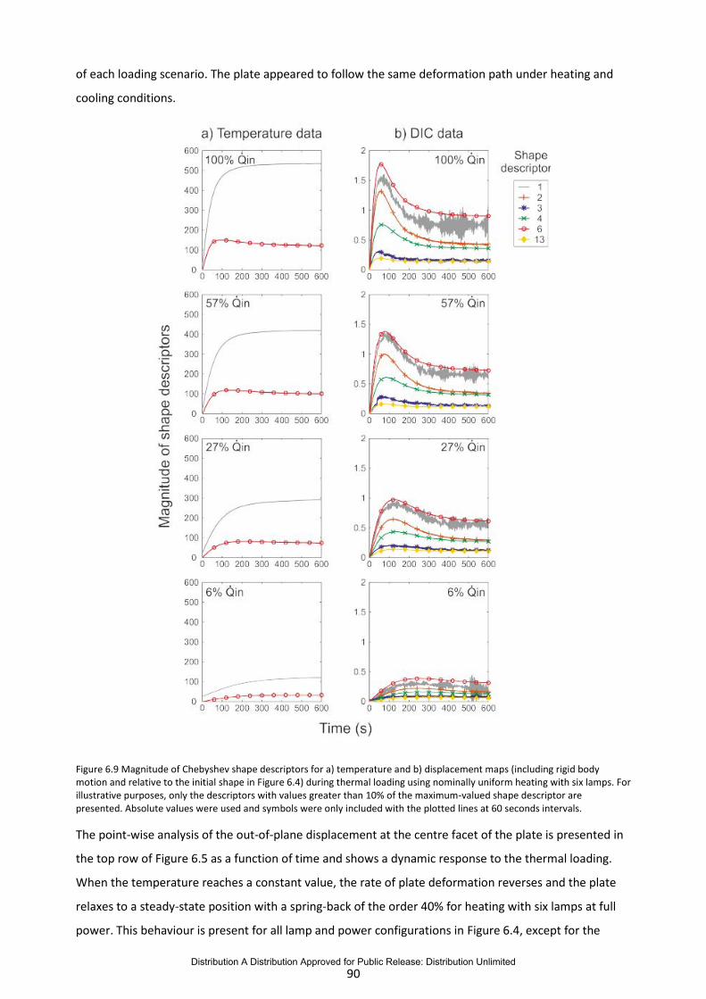
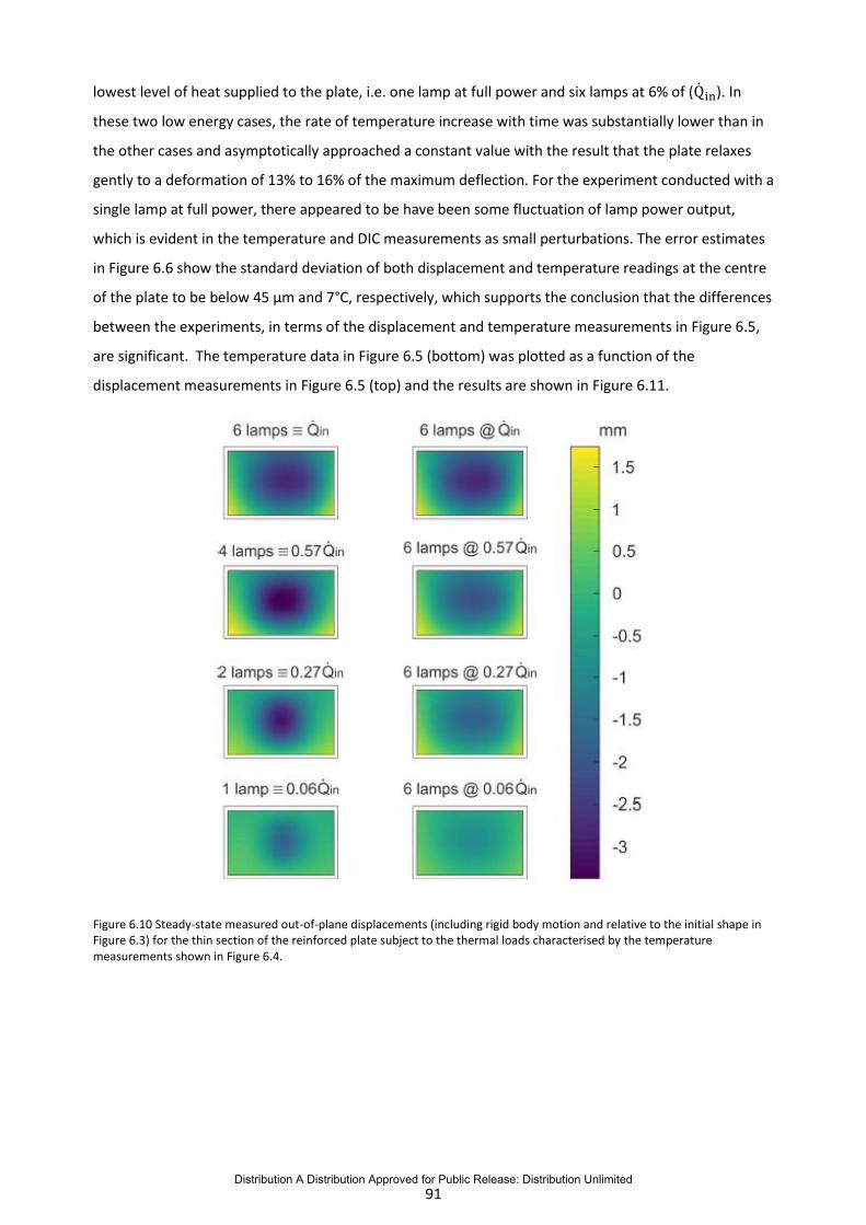
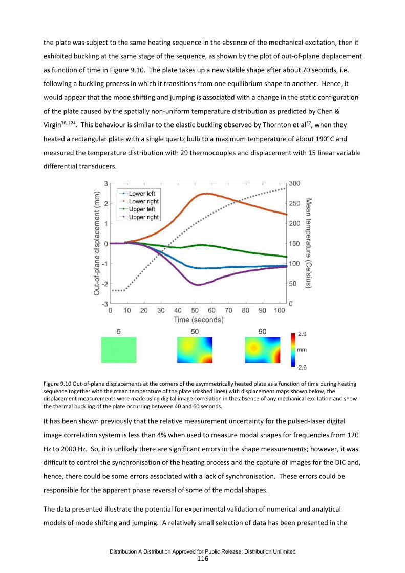
The work by Ana Catarina dos Santos Silva has been focused on the concurrent acquisition of full-field displacement and temperature data from aerospace-grade material plates subject to thermal and thermo-mechanical loading. A robust finite element (FE) model was also developed capable of predicting resonant frequencies and mode shapes for a plate under coupled non-uniform thermal and acoustic loading using temperature-dependent material properties and a realistic geometric representation of the initial curvature of the plate. Two-dimensional orthogonal decomposition was employed for compression of the full-field experimental data and validation of the FE model. Finally, the influence of non-uniform temperature distribution on the deformation of plates was further investigated using a 1mm plate with reinforced edges. The geometry was designed to emulate an aircraft's skin with the reinforced edges performing the function of stringers and ribs. Full-field deflection results for the reinforced plate showed it to behave as a dynamic system that buckles out-of-plane when heated before relaxing to a steady state. It was demonstrated that the out-of-plane displacement experienced by the plate is strongly influenced by the in-plane spatial distribution of temperature.
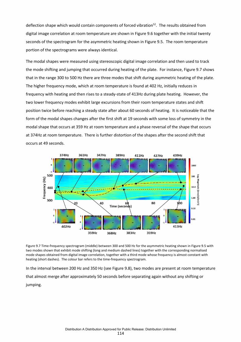
Elias Lopez Alba from University of Jaén, Spain, during his visit to the University of Liverpool in summer 2017, performed experiments to investigate the phenomenon of mode shifting and jumping that occurred in rectangular plate when subjected to asymmetrical heating beyond the point at which thermal buckling appears. Khurram Amjad as part of his post-doctoral work on this programme has investigated the use of thermoelastic stress analysis (TSA) technique for measuring full-field stresses from a plate subject to acoustic loading. There has been a lack of clarity in the literature about the interpretation of TSA data in obtaining both the mode shape and the quantitative stress information. Results from TSA and pulsed-laser DIC were compared to show that it is possible to use TSA for simultaneous acquisition of mode shape and stresses under loading conditions investigated by Silva and Alba. Three-dimensional (3D) orthogonal decomposition algorithm was employed to extend the validation framework to volumetric datasets. The newly developed decomposition algorithm was successfully applied for the compression of the measured and FE predicted data on a vibratory response of an aerospace panel and quantitative validation of the FE model.
Please direct any questions regarding the content of this report to Eann Patterson ([email protected])
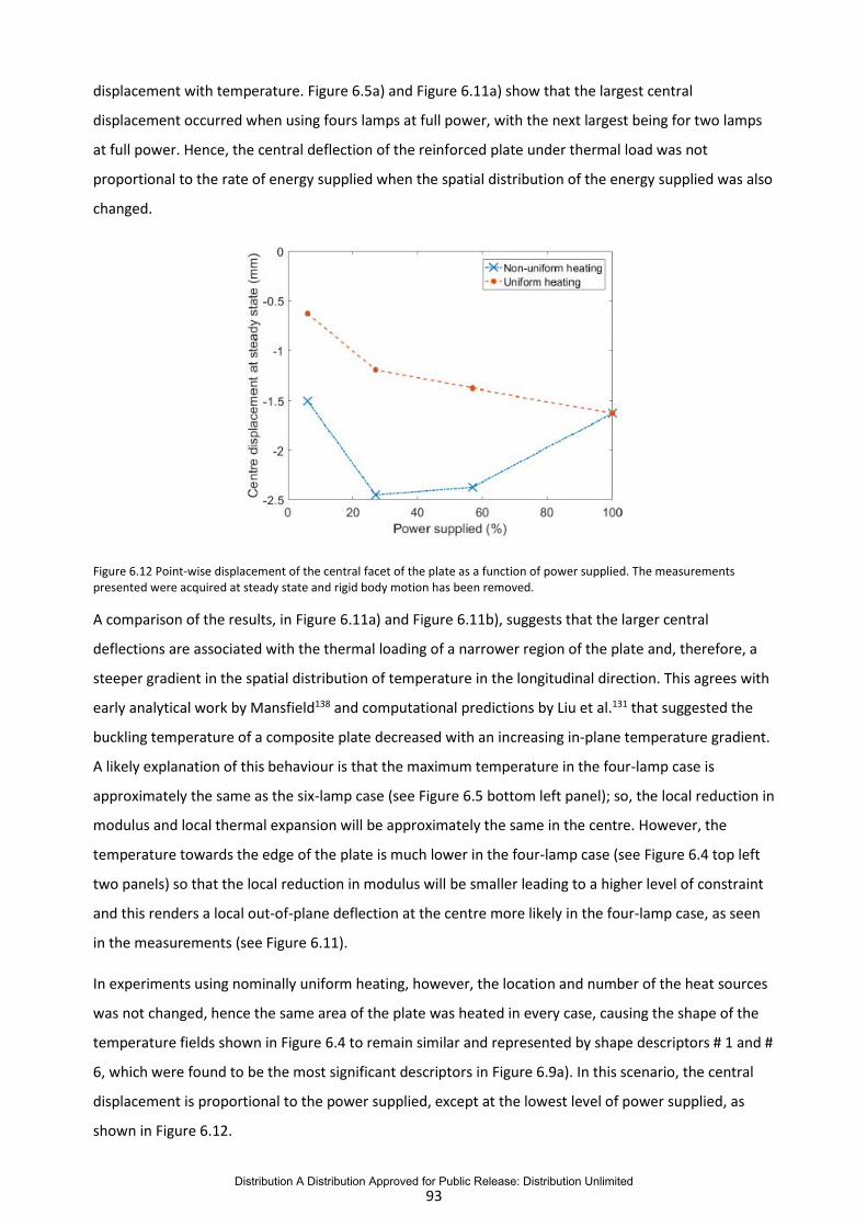
Distribution A Distribution Approved for Public Release: Distribution Unlimited
iii
Table of Contents
Summary / Abstract ....................................................................................................................................... i
Table of Contents ......................................................................................................................................... iii
List of Figures .............................................................................................................................................. vii
List of Tables ............................................................................................................................................... xv
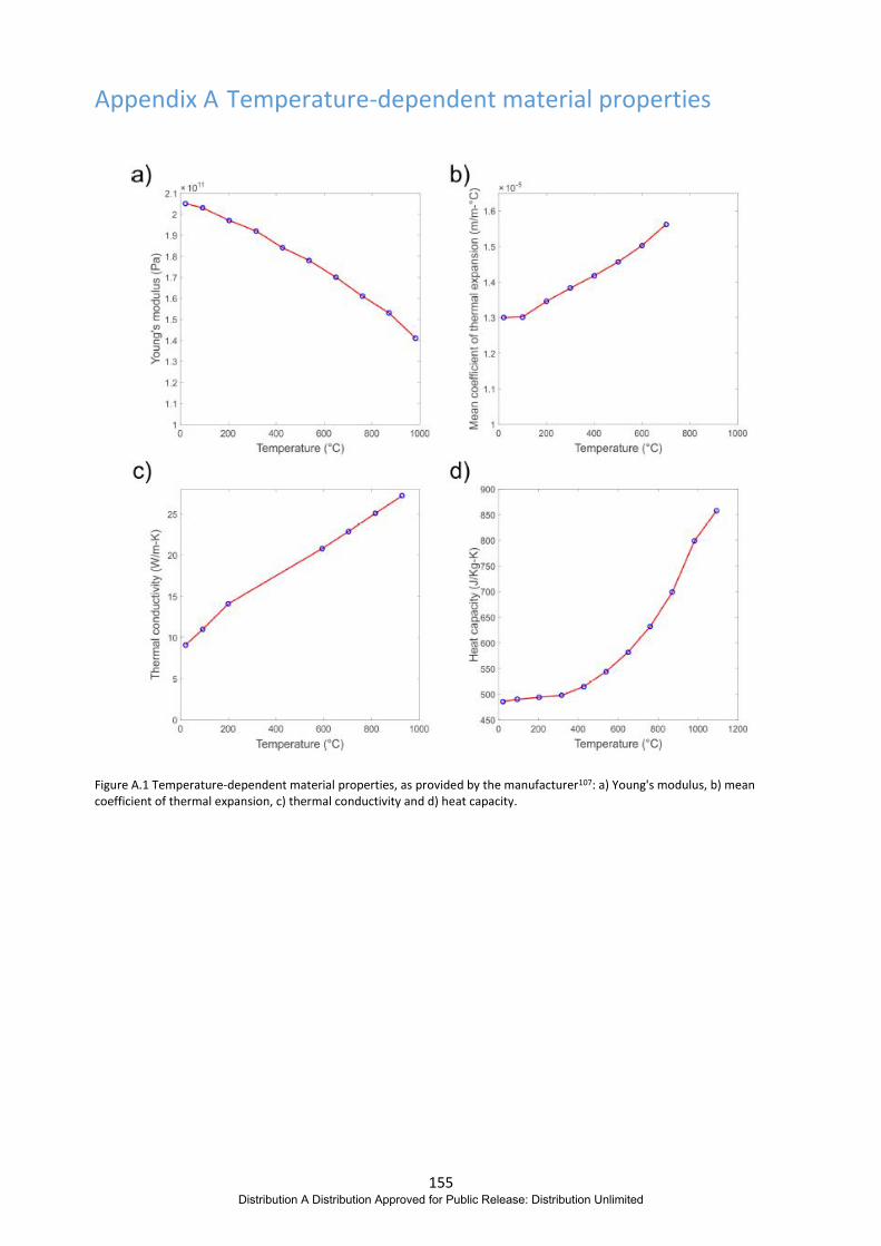
Appendix A Temperature-dependent material properties .................................................................. 155
Appendix B Original and simplified material models ........................................................................... 156
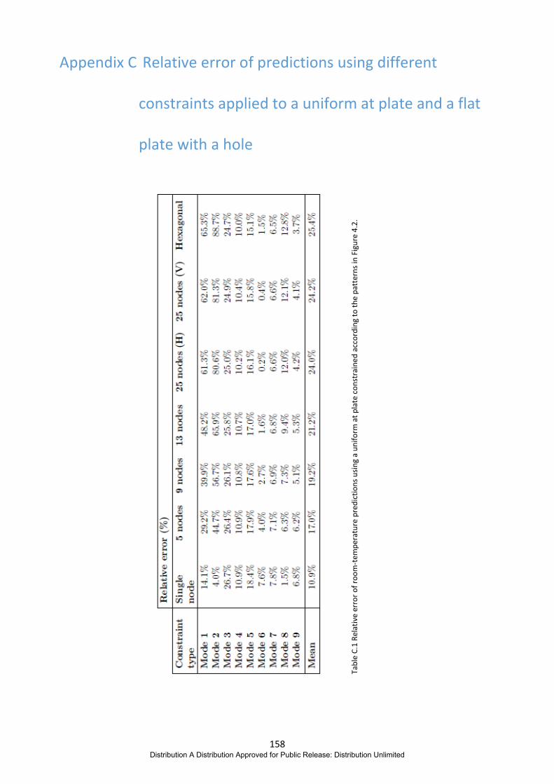
Appendix C Relative error of predictions using different constraints applied to a uniform at plate and
a flat plate with a hole .............................................................................................................................. 158
Appendix D Verification of resonant frequency predictions using a temperature-dependent material
model against literature ........................................................................................................................... 160
Appendix E Resonant frequency predictions using linear and non-linear solvers to calculate the effect
of a transient thermal load up to buckling ............................................................................................... 166
Appendix F Experimentally-acquired resonant frequency results of a thin plate ............................... 167
Appendix G List of Journal Publications................................................................................................ 170
Distribution A Distribution Approved for Public Release: Distribution Unlimited
vii
List of Figures
Figure 1.1 Development of a boundary layer over a flat plate. Adapted from 6. ......................................... 3
Figure 2.1 Non-dimensional surface and contour plot of plate buckling at a non-dimensional
temperature of 209.25 °C. From Mead35. ..................................................................................................... 8
Figure 2.2 Experimental setup used by Thornton et al. in the thermal loading of a Hastelloy X plate.
Adapted from Thornton et al.52. ................................................................................................................. 14
Figure 3.1 Schematic representation of the DIC process in which an undeformed facet in the reference
image is mapped onto a deformed facet in an image acquired post-loading. ........................................... 26
Figure 3.2 Discrete grey level representation of intensity values for a 16 x 16 pixel array. Image credit.
The b) Three-dimensional, c) bi-linear and d) bi-cubic spline representations of the same pixel array are
Distribution A Distribution Approved for Public Release: Distribution Unlimited
viii
Figure 4.8 Temperature distribution equivalent to Berke et al. 10, computed using a custom MATLAB
script, b) Temperature map at buckling point (Tcr) and c) the corresponding buckled shape, which has
been normalised between 1 (red) and -1 (dark blue). ................................................................................ 43
Figure 4.9 Predicted resonant frequencies with thermal load using the transient model in which a flat
plate was heated up to 110% of Tcr, which is shown in Figure 4.8 b). ....................................................... 43
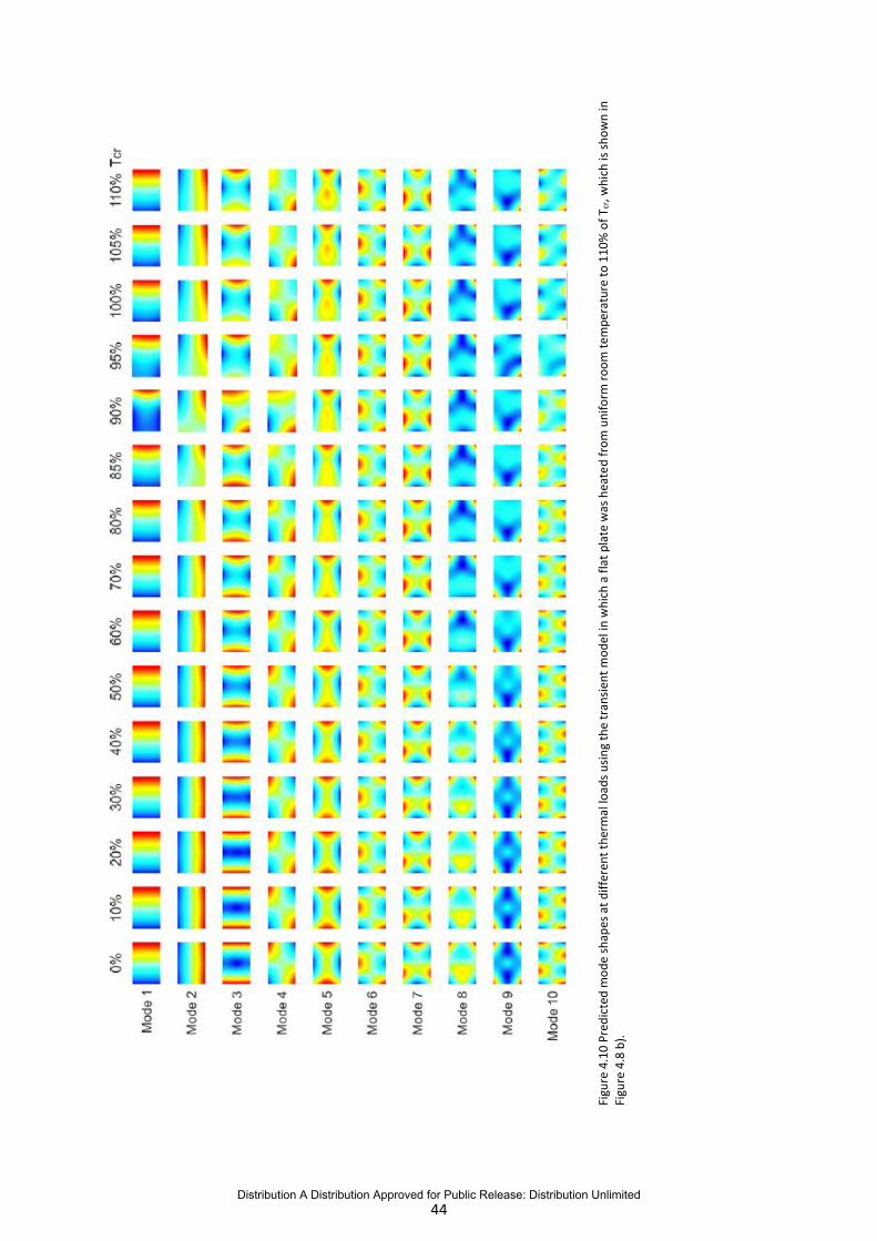
Figure 4.10 Predicted mode shapes at different thermal loads using the transient model in which a flat
plate was heated from uniform room temperature to 110% of Tcr, which is shown in Figure 4.8 b). ....... 44
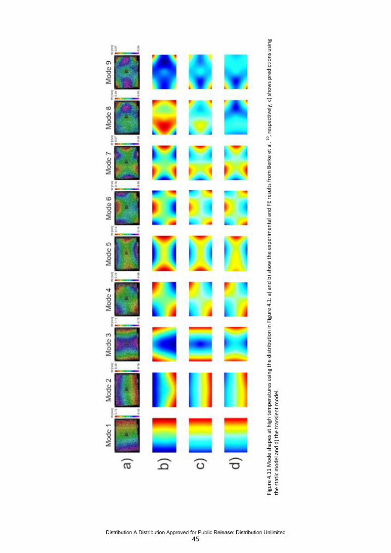
Figure 4.11 Mode shapes at high temperatures using the distribution in Figure 4.1: a) and b) show the
experimental and FE results from Berke et al. 10, respectively; c) shows predictions using the static model
and d) the transient model. ........................................................................................................................ 45
Figure 4.12 High-temperature, resonant frequency predictions from multiple models (top) and the
relative error of each one against experimental data from Berke et al. 10 (bottom). ................................ 46
Figure 4.13 Macroscale, measured plate geometry used in the transient thermal loading from a uniform
room temperature to the temperature distribution in Figure 4.8 b). ........................................................ 48
Figure 4.14 Predicted resonant frequencies with thermal load using the transient model in which an
imperfect plate was heated up to Tcr, shown in Figure 4.8 b). .................................................................. 48
Figure 4.15 Predicted mode shapes with thermal load using the transient model in which a measured
plate geometry was heated up to Tcr, shown in Figure 4.8 b). ................................................................... 49
Figure 4.16 High-temperature resonant frequencies as a function of room-temperature results using the
developed models and the results from Berke et al. 10. ............................................................................. 51
Figure 4.17 Predictions of in-plane and out-of-plane deformation of an ideally at plate (top) and plate
with measured geometry (bottom) using the transient model to load the structures up to Berke et al.'s10
temperature distribution in Figure 4.8. ...................................................................................................... 53
Figure 5.1 Photograph of the plate showing the painted speckle pattern used for digital image
correlation (DIC). Image from the left camera of the stereo-vision system shown. .................................. 57
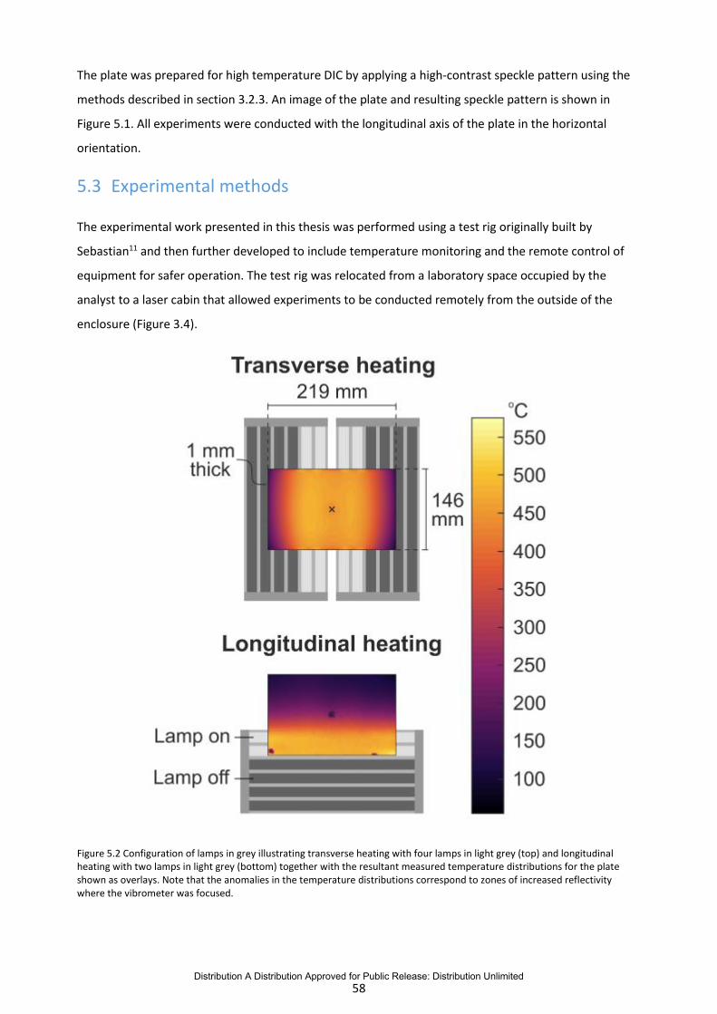
Figure 5.2 Configuration of lamps in grey illustrating transverse heating with four lamps in light grey
(top) and longitudinal heating with two lamps in light grey (bottom) together with the resultant
measured temperature distributions for the plate shown as overlays. Note that the anomalies in the
temperature distributions correspond to zones of increased reflectivity where the vibrometer was
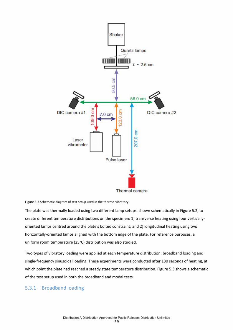
Figure 5.8 Measured (DIC) displacement maps for the test plate subject to the three temperature
regimes: room temperature (left), transverse heating of the centre of the plate (middle) and longitudinal
heating on one edge (right). All displacements are in mm. ........................................................................ 64
Figure 5.9 Predicted (FE) mode shapes for the test plate subject to the three temperature regimes: room
temperature (left), transverse heating of the centre of the plate (middle) and longitudinal heating on
one edge (right). ......................................................................................................................................... 66
Figure 5.10 Finite element shape computed using DIC contour measurements of the plate at room
Figure 5.12 Measured (solid bars) and predicted (shaded bars) resonant frequencies for a) uniform room
temperature; b) transverse heating of the centre of the plate; c) longitudinal heating on one edge.
Relative errors of predictions against measurement data are shown in parenthesis. ............................... 68
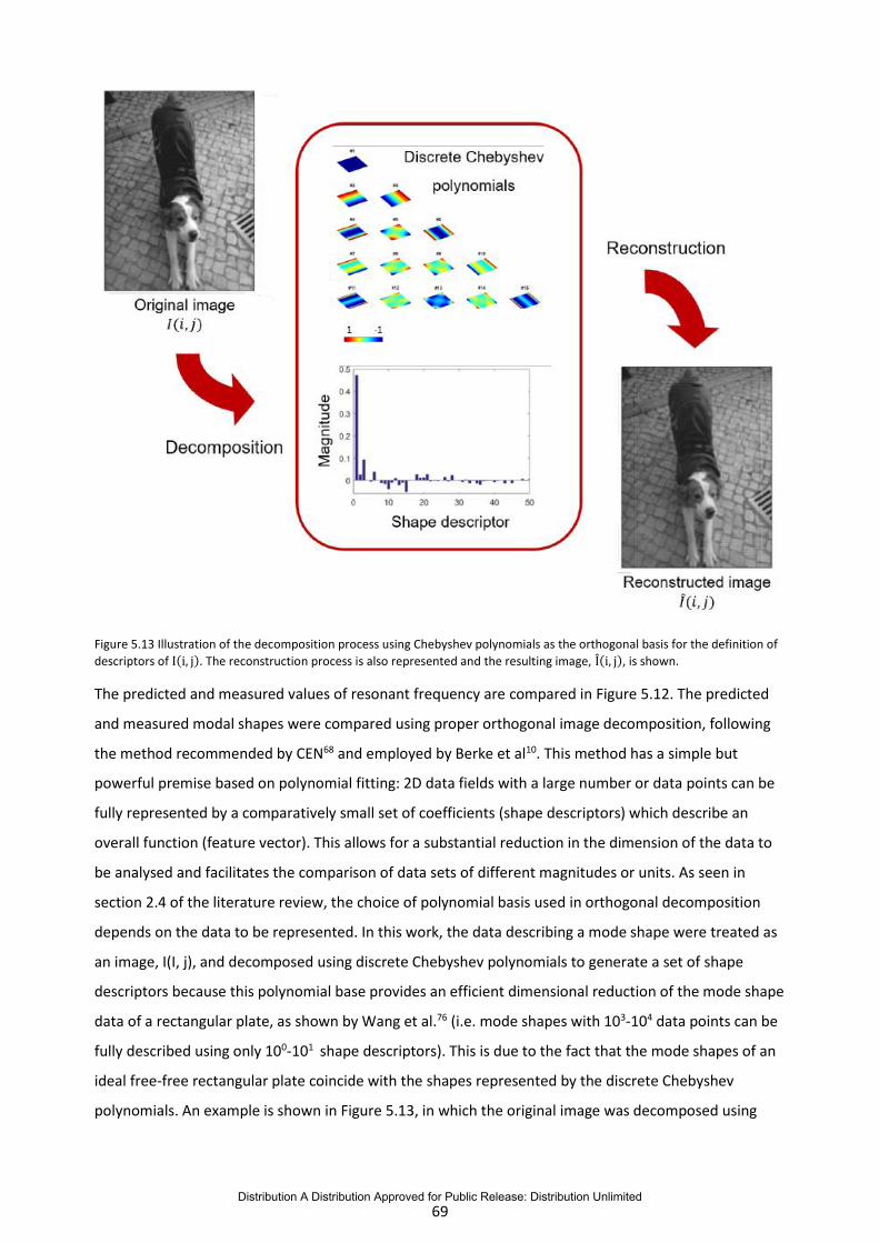
Figure 5.13 Illustration of the decomposition process using Chebyshev polynomials as the orthogonal
basis for the definition of descriptors of Ii, j. The reconstruction process is also represented and the
resulting image, Ii, j, is shown. .................................................................................................................... 69
Figure 5.14 Comparison of Chebyshev coefficients from the orthogonal decomposition of measurements
(horizontal axis) and predictions (vertical axis) data. Fifty Chebyshev kernels were used in the
decomposition of the measurement and prediction data. The first kernel was excluded from the plots as
it describes rigid out-of-plane translation only and is unrelated to the deformation of the plate. ........... 70
Figure 5.15 Predicted resonant frequencies using a temperature-dependent material model plotted
against experimental results. ...................................................................................................................... 71
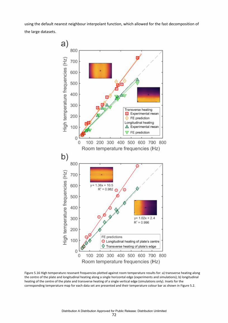
Figure 5.16 High temperature resonant frequencies plotted against room temperature results for: a)
transverse heating along the centre of the plate and longitudinal heating along a single horizontal edge
(experiments and simulations); b) longitudinal heating of the centre of the plate and transverse heating
Distribution A Distribution Approved for Public Release: Distribution Unlimited
x
of a single vertical edge (simulations only). Insets for the corresponding temperature map for each data
set are presented and their temperature colour bar as shown in Figure 5.2. ........................................... 72
Figure 5.17 Measured deformed shape of the plate in the absence of mechanical excitation but
following the transverse heating along the centre of the plate (top) and of a single longitudinal edge
(bottom). The datasets have been normalised between -1 (dark purple) and 1 (yellow) because the
energy inputs in the two cases are different and hence the absolute deformations are not directly
comparable. Missing DIC data due to the bolted constraint has been interpolated using the cubic
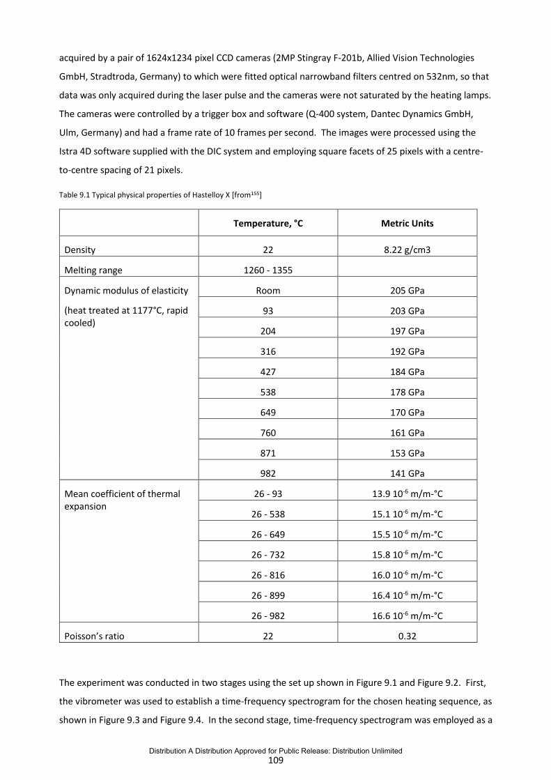
Table 9.1 Typical physical properties of Hastelloy X [from155] .................................................................. 109
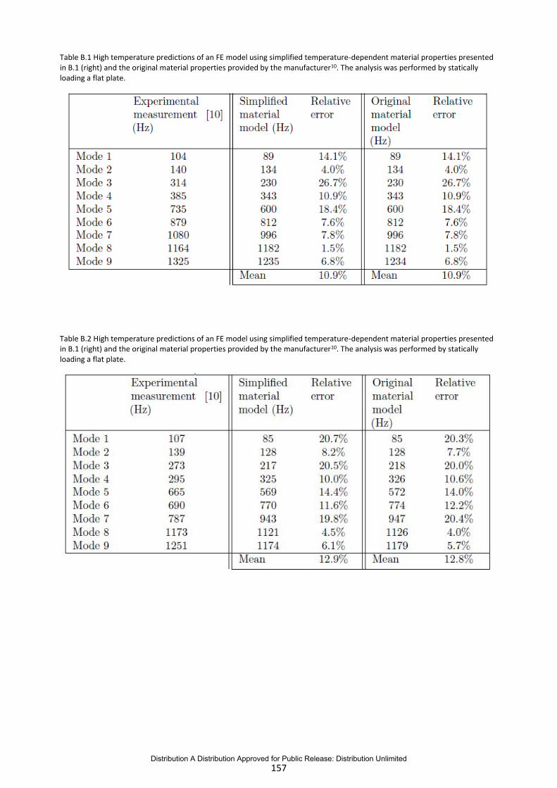
Table B.1 High temperature predictions of an FE model using simplified temperature-dependent
material properties presented in B.1 (right) and the original material properties provided by the
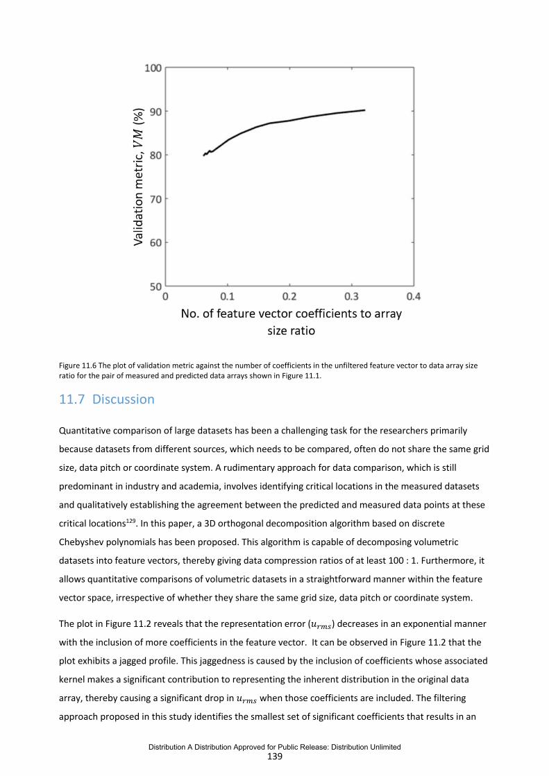
manufacturer10. The analysis was performed by statically loading a flat plate. ...................................... 157
Table B.2 High temperature predictions of an FE model using simplified temperature-dependent
material properties presented in B.1 (right) and the original material properties provided by the
manufacturer10. The analysis was performed by statically loading a flat plate. ...................................... 157
Table C.1 Relative error of room-temperature predictions using a uniform at plate constrained according
to the patterns in Figure 4.2. .................................................................................................................... 158
Table C.2 Relative error of room-temperature predictions using a flat plate with a hole constrained
according to the patterns in Figure 4.3..................................................................................................... 159
Table D.1 Resonant frequencies for CCCC boundary conditions. The relative difference was calculated
with respect to predictions published by Jeyaraj et al.33. ......................................................................... 160
Table D.2 Resonant frequencies for CCFC boundary conditions. The relative difference was calculated
with respect to predictions published by Jeyaraj et al. 33. ........................................................................ 161
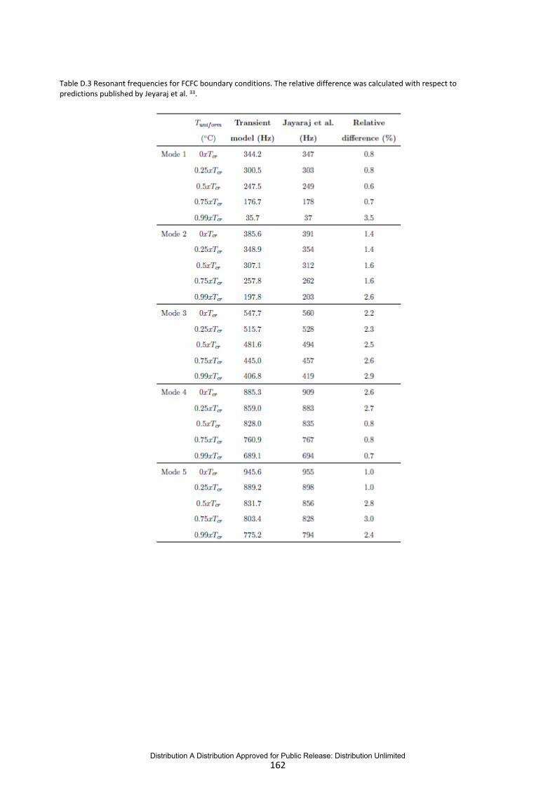
Table D.3 Resonant frequencies for FCFC boundary conditions. The relative difference was calculated
with respect to predictions published by Jeyaraj et al. 33. ........................................................................ 162
Distribution A Distribution Approved for Public Release: Distribution Unlimited
xvi
Table D.4 Resonant frequencies for CFFC boundary conditions. The relative difference was calculated
with respect to predictions published by Jeyaraj et al. 33. ........................................................................ 163
Table D.5 Resonant frequencies for SSSS boundary conditions. The relative difference was calculated
with respect to predictions published by Jeyaraj et al.33. ......................................................................... 164
Table F.1 Resonant frequency results acquired at room temperature and corresponding predictions
using a finite element (FE) model with temperature-dependent material properties ............................ 167
Table F.2 Resonant frequency results acquired when transversely heating the plate and corresponding
predictions using a finite element (FE) model with temperature-dependent material properties ......... 168
Table F.4 Resonant frequency results acquired when longitudinally heating the plate and corresponding
predictions using a finite element (FE) model with temperature-dependent material properties. ........ 169
Distribution A Distribution Approved for Public Release: Distribution Unlimited
1
Chapter 1 Introduction
1.1 Programme Overview
This is a final report on a 46-month programme conducted at the University of Liverpool (UoL) in
collaboration with Professor John Lambros at the University of Illinois at Urbana-Champaign (UIUC) and
supported by the US Air Force. The long-term goal of this collaborative work is the understanding and
modelling of the coupled thermoacoustic fatigue failure of aircraft structures and developing a
validation framework for the complex high-end numerical models, which would lead to the eventual
success of a “digital twin” concept.
Currently there is only limited structural level validation quality data available for cases of extreme
thermoacoustic loading. Validation quality data has different, and often more stringent, requirements
than experimental data associated with the investigation of physical phenomena on a laboratory scale.
For example, as the number of actual experiments may be limited, there is a need to capture as much
information as possible from a single experimental configuration, implying that many different
experimental techniques could be needed simultaneously. There is also a need for three-dimensional
(3D) information of stress and strain over large areas of the structure, and data acquisition over many
length and time scales may be required. The AFRL/RQ has several unique facilities that could be used for
the validation of simulations being developed by the collaborative efforts of the AFRL in-house
Structural Sciences Center (SSC) and the present research team. These facilities, the Combined
Environment Facility (CEAC), and its smaller counterpart, the Sub-Element facility (SEF), are capable of
producing sustained acoustic loading on a structural panel while maintaining variable thermal loading of
up to 1,650°C (3,000°F) by means of quartz lamp heating. These are ideal devices for the performance of
such thermoacoustic experiments. However, at the start of this programme there was nothing
formulized, either in terms of techniques or methodology or even understanding, that can meet the
stringent experimental validation requirements of SSC. The reason was the existence of multiple
knowledge gaps in all three areas: experimental techniques for thermoacoustic fatigue assessment, in-
depth understanding for appropriate thermoacoustic failure model development, and finally
methodologies for multi-scale multi physics validation. The work carried at UoL out as part of this 46-
month project has addressed key aspects of all of the three above-mentioned areas.
1.2 Report structure
The core of this report (Chapters 2-8) is the PhD thesis submitted by Ana Catarina dos Santos Silva in
September 2019 and successfully defended in November 2019. Her work was focused on investigating
the effects of coupled thermal and acoustic loading on aerospace grade metallic panels. Acquired
Distribution A Distribution Approved for Public Release: Distribution Unlimited
2
experiment data was used in the development and validation of computational models which aimed to
predict the structural response of the panels when subjected to a range of temperature distributions. A
self-contained Chapter 9 describes the work carried out by Elias Lopez Alba when he visited UoL from
University of Jaén, Spain in summer 2017. He performed experiments to investigate the phenomenon of
mode shifting and jumping that occurred in rectangular plate subject to asymmetrical heating beyond
the point at which thermal buckling appears. The last two self-contained chapters of this report are
contributed by Khurram Amjad who worked on this project as a post-doctoral researcher between
October 2017- December 2017 and December 2018 - September 2019. Chapter 9 describes the
investigation on the use of thermoelastic stress analysis technique for simultaneously measuring full-
field stresses and determining mode shapes in conditions investigated by Silva and Alba. A novel
approach for quantitative validation of volumetric datasets is described in Chapter 10. This validation
approach, which was partly developed in support of the work on a separate AFOSR grant (FA9550-17-1-
0272), is applicable to volumetric data sets with any combination of spatial and temporal variation along
three orthogonal dimensions of the volume. A list of publications originating from the work performed
under this grant is provided in Appendix G provided at the end of this report. The remainder of this
chapter contains the sections from the introduction chapter of Silva’s PhD thesis.
1.3 Motivation
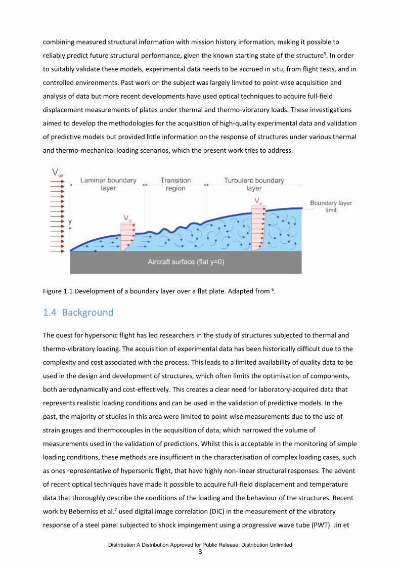
When the speed of a travelling aircraft exceeds the speed of sound, environmental conditions lead to
extreme loading scenarios that significantly shorten the lifecycle of materials and structures. In
supersonic and hypersonic flight, aircraft structures reach high temperatures due to aerodynamic
heating1, which are coupled with a broad spectrum of acoustic and vibratory loads generated by
fluctuating air pressures and high velocity gradients that characterise the aircraft's boundary layer
(illustrated in Figure 1.1). The aerodynamic heating is not uniform across the surfaces of the aircraft,
being particularly significant at its leading edges and creating severe temperature gradients across the
structure. Thermal and acoustic loads from the engine add to the complexity of this highly transient
environment, making it often difficult to identify which load or combination of loads is responsible for
component failure2. Thin-gauge components, such as the aircraft skin, are especially affected by high
thermal stresses which may cause a reduction or loss of structural stability as a result of the
development of in-plane compressive stresses3. Therefore, despite not being well understood, the effect
of high temperatures and vibro-acoustic loads heavily influence both the analysis and design of
supersonic and hypersonic aircrafts4.
The difficulty in obtaining measured data relevant to the study of aerospace structures under hypersonic
conditions makes it crucial to implement ways to predict material and structural responses throughout a
component's lifecycle. This can be achieved using simulation methods that are continuously being
revised and improved. Ideally, future developments will lead to predictive response models capable of
Distribution A Distribution Approved for Public Release: Distribution Unlimited
3
combining measured structural information with mission history information, making it possible to
reliably predict future structural performance, given the known starting state of the structure5. In order
to suitably validate these models, experimental data needs to be accrued in situ, from flight tests, and in
controlled environments. Past work on the subject was largely limited to point-wise acquisition and
analysis of data but more recent developments have used optical techniques to acquire full-field
displacement measurements of plates under thermal and thermo-vibratory loads. These investigations
aimed to develop the methodologies for the acquisition of high-quality experimental data and validation
of predictive models but provided little information on the response of structures under various thermal
and thermo-mechanical loading scenarios, which the present work tries to address.
Figure 1.1 Development of a boundary layer over a flat plate. Adapted from 6.
1.4 Background
The quest for hypersonic flight has led researchers in the study of structures subjected to thermal and
thermo-vibratory loading. The acquisition of experimental data has been historically difficult due to the
complexity and cost associated with the process. This leads to a limited availability of quality data to be
used in the design and development of structures, which often limits the optimisation of components,
both aerodynamically and cost-effectively. This creates a clear need for laboratory-acquired data that
represents realistic loading conditions and can be used in the validation of predictive models. In the
past, the majority of studies in this area were limited to point-wise measurements due to the use of
strain gauges and thermocouples in the acquisition of data, which narrowed the volume of
measurements used in the validation of predictions. Whilst this is acceptable in the monitoring of simple
loading conditions, these methods are insufficient in the characterisation of complex loading cases, such
as ones representative of hypersonic flight, that have highly non-linear structural responses. The advent
of recent optical techniques have made it possible to acquire full-field displacement and temperature
data that thoroughly describe the conditions of the loading and the behaviour of the structures. Recent
work by Beberniss et al.7 used digital image correlation (DIC) in the measurement of the vibratory
response of a steel panel subjected to shock impingement using a progressive wave tube (PWT). Jin et
Distribution A Distribution Approved for Public Release: Distribution Unlimited
4
al.8 have also used DIC in the monitoring of deformation of a thermally-stressed composite panel.
Abotula et al.9, Berke et al.10 and Sebastian11 used different heating methods to impart high
temperatures to small Hastelloy X plates which were also subjected to either shock-wave loading or
vibro-acoustic excitation. The work cited above has developed a means to gather experimental data for
the validation of predictive models of aerospace components; it yielded significant findings on the
dynamic behaviour of thermally stressed plates, prompting further developments on the topic. As large
strains associated with resonant modes and large displacements contribute to the fatigue of
components and can severely shorten their lifecycle, it is critical for the robust design and maintenance
of an aircraft to develop computational models which are capable of providing reliable predictions of
structural response. Therefore, the present project builds upon the work previously undertaken by
focusing on the characterisation of structural responses associated with thermal and thermo-vibratory
loading and the development of finite element (FE) models that can adequately describe them.
1.5 Aims and Objectives
The aim of this PhD research project was to investigate the effects of thermal and thermo-vibratory
loading on aerospace-grade metallic panels in laboratory conditions. Data acquired from experiments
was used in the development and validation of computational models which aimed to predict the
structural response of the panels when subjected to a range of temperature distributions. As the driving
force behind this work is the future merger of mission history data with structural information acquired
in-situ, all investigations were kept at a component level (macroscale). To achieve the aim of this
project, the following objectives have been set:
1. To experimentally study the effect of temperature on the dynamic response of aerospace
panels, particularly the influence of non-uniform temperature distributions.
2. To develop and validate a computational solid mechanics model with temperature-dependent
material properties, capable of predicting the behaviour of components when subjected to and
combined thermo-vibratory loads;
3. To perform experimental thermal and thermo-vibratory loading of aerospace-grade metal
panels in order to acquire full-field, high-quality displacement and temperature data to be used
in the development and validation of predictive models;
Distribution A Distribution Approved for Public Release: Distribution Unlimited
5
Chapter 2 Literature Review
The structural behaviour of thin-walled structures has been a problem tackled by engineers since the
early days of aviation and the wood-steel-fabric biplane era12. The vast majority of this early work
focused on the effect of mechanical loads on plates and shells used in the construction of aircraft. After
World War II, however, the pursuit of supersonic fight brought to light the effect of elevated
temperatures induced by aerodynamic heating on the material selection and structural design
practices12. At transonic speeds, air compression and increased friction between the aircraft and the air
flow were identified to be the main mechanisms responsible for this local increase in temperatures1. In
1992, Thornton13 published a journal paper surveying the advancements in the analysis of thermal
structures from the first considerations for supersonic flight to the developments of hypersonic aircraft.
Thornton listed the ways in which elevated temperatures are detrimental to structural behaviour: 1) the
most evident effect is the decrease in Young's modulus with temperature, which decreases the ability of
the structure to withstand loads and reduces allowable stresses; 2) time-dependent material behaviour
such as creep can become a determining factor in material and structural design; 3) thermal stresses are
introduced due to existing structural constraints and non-uniform material expansion/contraction.
These stresses can deformation, alter structural dynamic behaviour, affect component fatigue life and
uniquely affect the stability of components.
Several research programs on the effect of combined thermo-mechanical loading in aerospace
structures have been sponsored by the United States (U.S.) government. The importance of research on,
what came to be known as the "thermal barrier", was first recognised in 1944 with the development of
the transonic aircraft, the Bell X-1, which reached Mach 1.94 in a 1957 research mission. Whilst data
acquired during such missions showed aircraft skin temperatures to be below 100 °C, the rapid increase
in speed above the sonic threshold demonstrated the need to consider aerodynamic heating. The first
program aimed at the development of a hypersonic aircraft ran from 1954 to 1968 and resulted in the
design and manufacture of three rocket-powered aircraft - the X-15. These were capable of flying at
altitudes of 10,000 feet (approximately 3,000 m) or higher and achieved speeds of Mach 5. Under these
conditions, data gathered on a 1965 mission showed the temperatures at the leading edges of the wings
to reach over 700 °C (1325 °F)14. The development of the successor of the X-15 started in 1982, after a
long period dedicated to more fundamental research. The U.S. government terminated the funding for
this project in 1994 and concept models of the X-30 National Aerospace Plane (NASP) were never
developed into a full-scale aircraft, which was intended to fly at speeds of Mach 2515. The program
yielded significant findings on high-temperature fatigue of materials and structures as the 1\3 concept
demonstrator was studied using a high-temperature wind tunnel. Results suggested real in-flight
airframe temperatures to exceed 1650 °C 16. The U.S. then faced a lack of a cohesive program of
Distribution A Distribution Approved for Public Release: Distribution Unlimited
6
hypersonic technology development as a series of research efforts followed the cancellation of the X-30
project in an attempt to keep research momentum throughout the 1990s. One such program resulted in
the Hyper-X or X-43A aircraft and used NASP technology to expedite its readiness level towards the
demonstration of hypersonic air-breathing propulsion in flight17. Three expendable X-43A vehicles were
built and tested in the early to mid-2000s. The first two test flights fell short of the accomplishments of
the third, which set the speed record for a jet aircraft at Mach 9.6. In 2006, McClinton gave a lecture on
the significance of data gathered during these test flights and showed measured surface temperatures
to have reached approximately 1090°C (2000°F) 18. In 2003, the U.S. Air Force Research Laboratory
began the design and development of a hypersonic aircraft powered by a jet engine: the X-51A
Waverider. A total of four aircraft were built, none of them being designed to be recovered after the
test flight (akin to the X-43A). The X-51A maiden flight took place in 2010 followed by two unsuccessful
attempts. In 2013, the final X-51A aircraft travelled more than 230 nautical miles in just over six
minutes, reaching a peak speed on Mach 5.1 19. Lane published information on the design criteria for the
X-51A20, which included considerations on the temperature range experienced by the vehicle's skin and
exhaust nozzle - from approximately 815 °C (1500 °F) to 1920 °C (3500 °F).
Whilst the data gathered in modern hypersonic research flights is not widely available to the public,
investigations into the effect of thermal and thermovibratory loads on aerospace structures have
continued. The vast majority of this work has been carried out using computational mechanics
simulations or analytical models due to the cost-effective nature of these investigations. Nevertheless,
results have provided important insights into the predicted aerothermal and acoustic loads to be
encountered by a vehicle travelling on a typical trajectory. One such example is the extensive analytic
work by Blevins et al.2, 21 which predicted aircraft panel temperatures to reach values of 1140-1790 °C,
depending on the airflow and ascent trajectory. Aeroacoustic loads due to boundary layer turbulence
were found to be between 130 and 145 dB, whilst engine noise was estimated to be as high as 170 dB. A
conference paper by Beberniss et al.7 noted high-cycle or sonic fatigue to occur in thin, lightly-damped
aircraft structures with vibrational modes below 500 Hz. Recent developments in optical techniques
have enabled the full-field acquisition of measurements, prompting further advances in the subject,
which are addressed later in this review.
As the aim of the work presented in this thesis includes both experimental and computational studies on
the effect of thermal loads on the dynamic behaviour of thin-walled panels, a brief review of the current
literature on experimental and numerical advancements is presented. The first part discusses the
contribution of past analytical and predictive work largely derived from studies on thermal buckling,
which is defined as a highly non-linear event in which transverse pressure and, or in-plane compressive
loads lead to a loss of structural stability and the change in the stable configuration of the component22.
The second part focuses on the findings and experimental advances in the modal analysis of panels
under thermo-vibratory loads; including the determination of the resonant frequencies of the structure
Distribution A Distribution Approved for Public Release: Distribution Unlimited
7
and the out-of-plane displacement maps that represent a pattern of vibration at those frequencies
(mode shapes).The third part of this review examines the current state-of-the-art in the experimental
thermal loading of panels and the effects of temperature on the deformation of these structures.
Finally, the fourth part gives an appraisal of the current techniques used in the analysis of full-field data,
acquired using optical techniques.
2.1 Analytical and computational studies on thermally and thermo-
mechanically loaded plates
Plate theory has been an extensively studied field of engineering, both analytically and computationally.
Existing work on analytical plate theory was compiled and collated by Leissa23 and published in 1969 by
NASA. In his monograph, Leissa presented a comprehensive set of results based on linear plate theory
for the resonant frequencies and corresponding mode shapes associated with the free vibration of
plates. This compendium includes different plate shapes, aspect ratios and boundary conditions. Major
contributors to the theory presented in Leissa's monograph were Timoshenko and Woinowsky-Kriege24.
These studies gave little to no consideration to the effect of temperature on the structural behaviour of
the analysed plates.
Early work by Lurie25 and Bailey26 found a clear relationship between resonant frequencies and loads
applied to the plate (mechanical and thermal loads, respectively). Following a linear approach in his
analytical study, Bailey's results suggested the first resonant frequency to decrease with temperature
until the stressed state of a cantilever is such that the structure buckles27. As such, 𝛥Tcr defines the state
of thermal stresses at which a component buckles and the resonant frequency corresponding to the first
free vibration mode becomes zero, leading to the "disappearance" of the mode. In his studies, Bailey26, 27
also noted that the resonant frequencies of certain modes are capable of moving across the frequency
spectrum during the thermal loading of a plate, enabling resonant modes to change position in the
frequency spectrum. Jones et al.28 built upon work done by Pal29-31 and Berger32 and obtained more
accurate analytical solutions for the static and dynamic behaviour of plates at elevated temperatures. A
recent study by Jeyeraj et al.33 on at plates confirmed a decrease in frequency for each resonant mode
when exposed to a uniform increase in temperature and under various boundary conditions: fully
clamped, simply supported and free edges. The "disappearance" of the first mode as the temperature
approached the critical buckling value was also witnessed. The authors performed detailed simulation
work on isotropic, rectangular plates using a combination of FE analysis and boundary element methods
(BEM) to predict the resonant frequencies and mode shapes of a flat plate at different stages of uniform
thermal loading, assuming temperature-independent material properties.
In 1973, replicating the linear analytical approach used by Bailey26 and Simons and Leissa34, Mead35
focused on the analytical and computational study of ideal at Kirchhoff plates, rectangular in shape and
Distribution A Distribution Approved for Public Release: Distribution Unlimited
8
with free edges. These were subjected to in-plane thermal stresses resulting from non-uniform
temperature distributions that were doubly symmetrical about the centrelines of the plates. Results
showed that the temperature at which the plate buckled was strongly dependent on the temperature
distribution applied to the plate. Mead built upon the fact the resonant frequencies of beams and plates
are known to vary depending on the loading conditions to which they are subjected, concluding in his
studies that compressive thermal stresses induced by high temperatures reduce the local stiffness while
tensile stresses at cold areas of the plate increase it. For simplicity, Mead assumed a constant Young's
modulus and a linear expansion coefficient. Mead verified that buckling of the centre of a plate is
associated with compressive stresses in the same region (Figure 2.1). These stresses stem from a
spatially-distributed thermal load imparted by highest temperatures at the centre of the plate.
Conversely, edge-buckling occurs when the centre of the plate is subjected to tensile stresses associated
with higher temperatures at the edges. Moreover, Mead found edge-buckling to occur at lower absolute
temperatures, as the free edges are less constrained by plate tension than the central region.
Figure 2.1 Non-dimensional surface and contour plot of plate buckling at a non-dimensional temperature of 209.25 °C. From Mead35.
Mead's analysis suggested that, with an increasing temperature in the centre of the plate relative to its
edges, there was an increase in the resonant frequencies for the doubly symmetrical and
antisymmetrical modes of a rectangular plate. His results also showed particular mode shapes to switch
frequencies in a phenomenon called mode shifting. Chen and Virgin36 further investigated this
phenomenon by combining an analytical approach with Finite Element (FE) analysis in the study of
thermally post-buckled, aluminium plates. These authors assumed material properties to be
temperature-independent when developing their model in ANSYS. Shell elements were programmed in
the model and simply-supported boundary conditions were simulated. Their predictions showed a
change in the resonant frequencies with temperature which demonstrated the dynamic instability of the
thermally buckled structure. Mode shifting was found to be absent in the post-buckled regime if the
plate underwent a second buckling event.
In recent years, more powerful computing facilities made the development of increasingly complex
mechanics models possible. One such example is the inclusion of temperature-dependent material
Distribution A Distribution Approved for Public Release: Distribution Unlimited
9
properties in FE-based simulations that can describe thermal softening under elevated temperatures
which has been adopted by several researchers. Ko37 predicted the post-buckled shapes of rectangular
plates subject to dome-shaped temperature distributions and found the critical temperature at which
buckling occurred; Ibrahim et al.38 studied the non-linear random response of functionally graded (FG)
panels under combined thermal and acoustic loads using a non-linear finite element model; while Talha
et al.39 investigated the random vibration response of FG plates and analysed the effect of uncertainty in
material properties on the frequency response. The majority of the relevant models using temperature-
dependent material has, in fact, focused on investigations of the vibratory response of FG structures by
modelling the thermal properties of their constituent materials40-43. However, none of these studies
investigated the effect of temperature on resonant frequencies and mode shapes of isotropic plates, for
which Berke et al.10 developed an FE-model based on small strains and a linear elastic response with no
thermal expansion or conduction included. The dependence of the Young's modulus on temperature
was introduced by Berke et al. by assigning specific values of modulus to nodes based on a discrete
temperature distribution, which was calculated from measured strain data and the material properties
published by the manufacturer. These authors also used full-field experimental techniques to acquire
measurements of the shape of the plate, which was a much more realistic approach to the geometric
model than idealised plates used in the other investigations discussed here. This has a very significant
influence in the resonant frequencies and mode shapes of the structure as shown by Murphy et al.44, 45
who tested a fully-clamped plate subjected to a uniform thermal load and compared experimental
measurements with theoretical results. By modelling an initial central detection of the plate44, their
results did not show the "disappearance" of resonant frequencies with an increase in temperature, as
predicted by Bailey27 and Jeyaraj et al.33 In fact, imperfections were proven to increase the structural
stiffness of the stressed plate. This was in line with Lurie's work25 which shows that a small deflection
specified as initial imperfection causes an increase in stiffness as the structure undergoes further
gradual detection with increasing load.
Cui and Hu46 developed a temperature-dependent theoretical model to predict the effect of uniform
heating on an ideal isotropic plate with a complex boundary condition: stick-slip-stop. This meant the in-
plane expansion of the plate was initially limited by normal or frictional forces, followed by a subsequent
slip and a final stop. Their results showed the resonant frequencies of the plate to be highly dependent
on the conditions that constrain the plate initially, before slipping occurs. A high level of initial
constraints was shown to lead to a decrease in the first three resonant frequencies of the plate when
subjected to a uniform temperature rise, particularly in the case of the first resonant mode. However,
when these constraining forces allowed the plate to expand more freely, the initial decrease in resonant
frequencies was followed by an increase before diminishing once again.
2.1.1 Conclusions
Distribution A Distribution Approved for Public Release: Distribution Unlimited
10
Extensive analytical and computational research has been carried out on the static and dynamic
behaviour of plates subjected to various loads and boundary conditions. Important conclusions have
been drawn from these studies, namely the strong influence of geometric non-linearities and boundary
conditions on the dynamic behaviour of thermally stressed plates; non-uniform temperature
distributions across components were shown to yield non-linear responses to thermal and thermo-
mechanical loading. However, it is important to highlight that very few studies have used temperature-
dependent material models in the study of resonant frequencies and mode shapes of isotropic plates.
The most interesting examinations carried out to date have been performed by Cui and Hu46 and Berke
et al.10, despite some identifiable limitations. Cui and Hu restricted their study to the analysis of
through-thickness gradients of an ideal plate, opting for a uniform in-plane temperature distribution.
Berke et al. compared their simulation results to experimental measurements and some differences
were observed between the predicted and experimentally determined resonant frequencies. These
discrepancies were possibly due the overly simplistic material model which did not include thermal
expansion or conduction, and therefore did not suitably replicate the thermal loading process. The
assumption of constant material characteristics throughout the thermal loading process has
repercussions on the geometric stiffness of the component and affects the predicted vibratory
response. Notably, most of the reviewed predictive studies did not include any attempt at validation by
comparison with measurements.
2.2 Experimental studies on vibro-acoustic loading of thermally
stressed plates
A limited amount of experimental research has been performed on the modal response of thermally
stressed plates. The majority of existing work has been performed using the Thermal Acoustic Fatigue
Apparatus (TAFA) at the NASA Langley Research Center. Ng and Clevenson47 performed experiments on
304.8 x 381 x 1.6 mm (12 x 15 x 0.063 in.) aluminium plates using the TAFA in order to study the random
motion of buckled plates when exposed to thermoacoustic loading. For their work, Ng and Clevenson
exposed the specimens to noise levels up to 160 dB using pressurised air supplied by two electro-
pneumatic modulators. Heating of the plates was achieved using twelve 2.5 kW quartz lamps.
Instrumentation on the aluminium plate consisted of thermocouples and strain gauges located on both
the front and back of the plate while the noise level was measured using microphones. The plate was
fully clamped at its edges using steel brackets for the mounting and experiments were conducted with
and without insulation between the plate and mounting frame. Non-uniform temperatures were
achieved for both the uninsulated (121.1°C at the plate's centre and 43.3°C at the edges) and insulated
(121.1°C centre temperature and approximately 87°C at the edges) experiments. Results showed the
increase or decrease in resonant frequencies of the plate when compared to room-temperature
conditions to depend on the magnitude of displacements induced by the thermal load; however, no
Distribution A Distribution Approved for Public Release: Distribution Unlimited
11
analysis of mode shapes was conducted. Whilst the experimental results agreed with the FEA
predictions for the fully-clamped uninsulated plate, the same was not achieved for the insulated plate
due to the non-linear properties of the insulating material which modified the plate's boundary
conditions. The uncertainty introduced by thermal insulation in the boundary conditions of the
specimen was also highlighted by Leatherwood et al.48 when using an equivalent experimental setup in
the thermo-acoustic loading of flat and blade-stiffened panels to failure. The recurrent failure of
instrumentation used in tests up to approximately 650°C (1200°C) clearly illustrated the complexity of
high-temperature experiments using contact methods for data acquisition.
In 1991, Snyder and Kehoe49 reported on experiments using a suspended aluminium plate subjected to
uniform, non-uniform and transient thermal loads. The plate was instrumented with 18 accelerometers
and 30 thermocouples and heated in an oven using an array of quartz lamps placed on one side of the
structure. A calibrated hammer was used to provide impact excitation to the plate. Their results showed
an increase in temperature, uniform or otherwise, to yield a reduction in resonant frequency for the first
four modes of the plate. Despite representing a considerable contribution to the field, this study was
restricted to small in-plane temperature gradients with maximum local temperatures just over 200°C,
similar to Ng and Clevenson47.
Istenes et al.50 studied the effect of thermal load on the dynamic behaviour of four fully-clamped panels
made from a graphite polymeric composite with different laminate layups. Strain was measured using
fourteen strain gauges mounted in symmetric pairs on both sides of the panels and in seven different
locations. A thermocouple was mounted at the centre of each panel to monitor their temperature and
an infrared imaging radiometer confirmed the temperature distribution across the specimens to be near
uniform. Clamping of the four edges of the panels was achieved using two steel support frames which
provided the clamping force needed when bolted together. The interface between the steel clamping
frame and the test specimen was insulated to minimise the thermal dissipation via conduction between
the specimen and the rig. An electrodynamic shaker was used to mechanically load the specimens whilst
heating was provided by two 100W lamp banks with 8 lamps each, located on one side of the panels.
Each specimen underwent broadband loading at room temperature followed by the narrowband
excitation of the first two vibration modes. The same procedure was applied in experiments at 121.1°C,
148.9°C and 176.7°C. Their results suggested high in-plane strains introduced by the thermal load to act
as a stabiliser to the motion of the plates when vibrating about their buckled position.
In two complimentary studies, Murphy et al.44, 45 studied the resonant frequencies of an AISI 321
stainless steel plate subjected to thermo-acoustic loading. Experiments were conducted at the TAFA
(see above) where a plate of dimensions 381 x 304.8 x 3.175 mm was fully clamped onto a side wall of
the test area and thus subjected to a grazing acoustic load. Placed opposite to the specimen and across
the TAFA chamber, a set of ten quartz lamps was used to provide a radiant thermal load. The clamp was
Distribution A Distribution Approved for Public Release: Distribution Unlimited
12
continuously cooled using a built-in water channel in order to avoid a change in the boundary conditions
of the specimen due to thermal expansion of the frame; an insulating blanket was sandwiched between
the plate and the clamp for the same purpose. The temperature was monitored using several
thermocouples distributed across the width and length of the plate. The output of these thermocouples
was used to provide feedback to a control system which adjusted the energy distribution of the banks of
lamps so that a near-uniform temperature distribution was achieved across the plate. Displacement and
strain data was measured using strain gauges and a scanning laser vibrometer, with the latter being
used to create a map of the velocity magnitude and phase across the specimen. The dynamic behaviour
of the plate was recorded at room temperature and the process repeated at several different intervals
of the thermal loading. The authors compared the experimental results with analytical predictions and
highlighted the importance of initial imperfections on analytical results, as discussed in section 2.1. They
also recognised there were some inevitable in-plane displacements between the clamping frame and
test plate due to the ceramic coating used for insulation purposes. This meant the fully-clamped
boundary conditions in the FE model were not reproduced experimentally.
Further experiments on fully-clamped aluminium plates were performed by Geng et al.51 and their
results showed a moderate increase in uniform temperature (approximately 20°C) to decrease the
resonant frequencies of the plate. The first five resonant modes of the plate were identified using an
impact hammer test at room temperature before increasing the thermal load and repeating the process.
A modal exciter was used to dynamically load the plate at resonant frequencies whilst a set of
accelerometers measured the vibratory response. The authors attributed the decrease in resonant
frequencies to the thermal softening of the material and compressive stresses accumulated in the
structure due to the limited thermal expansion allowed in fully-clamped conditions. Complimentary
simulations performed by the authors correlated well with their experimental findings; however, this
computational work also suggested initial deflections of the plate to greatly affect its resonant
frequencies and could even counteract the effect of thermal softening.
Recent investigations departed from the use of contact instruments for the acquisition of experimental
data and opted for full-field optical methods. Beberniss et al.7 used stereoscopic image correlation to
capture the dynamic response of a thin panel subjected to shock impingement. Whilst no thermal load
was considered initially, the authors conducted a follow-up investigation4 in which the panel was
exposed to a heated airflow, reaching non-uniform temperatures of 80°C. These studies helped the
authors in the development and planning of future experiments as preliminary results showed the panel
to present highly non-linear behaviour under combined loading. Similarly, Berke et al.10 showed the
change of resonant frequencies of a 120x80x1 mm Hastelloy X plate under thermal load to vary from
mode to mode. The authors conducted experiments using an induction coil to heat the specimen and a
shaker to provide vibratory excitation. A non-uniform in-plane temperature distribution was achieved
and estimated using high-temperature strains measurements divided by the material's temperature-
Distribution A Distribution Approved for Public Release: Distribution Unlimited
13
dependent coefficient of thermal expansion; magnitudes were determined to have reached
approximately 600°C. Mode shapes were acquired using high-speed stereoscopic DIC. Results showed
most of the resonant frequencies of the small plate to decrease with thermal load but that was not the
case for every mode.
2.2.1 Conclusions
The work described above has greatly contributed to the acquisition of experimental data pertaining to
the resonant frequencies and mode shapes of plates and panels under combined thermo-vibratory
loading. The vast majority of these investigations used point-based techniques for the acquisition of
data, particularly temperature data, which limited the scope and depth of the studies. Particular
attention was given to the effect of insulating material in imparting elasticity to fully-clamped boundary
conditions, which hinders the development of predictive models that suitably replicate experiments.
Similar to the findings of analytical studies, experimental results showed geometric imperfections in the
plates to influence the increase or decrease of its resonant frequencies with thermal load. Most
published work was performed using fully-clamped plates under uniform temperatures and showed
evidence of the thermal softening of the material leading to a decrease in resonant frequencies.
However, results from Berke et al.10 using a free-edge plate subjected to non-uniform heating suggest
the frequency of some resonant modes to increase at elevated temperatures. A single temperature
distribution was used in this investigation, which does not provide a comprehensive study on the
resonant frequencies and mode shapes of the plate when exposed to a change in in-plane temperature.
This constitutes a particular point of interest as the predictions by Jeyaraj et al.33 suggest a change in
mode shapes with thermal load when one or more edges are free.
2.3 Experimental advances on the influence of thermal load on the
deformation of panel structures
Experimental work on thermally stressed components has been limited, partly due to the complexity
behind the necessary experimental setup. The acquisition and analysis of experimental data have also
been restricted by available techniques, which target the gathering of point-wise data and neglect full-
field phenomena.
Thornton et al.52 studied the elastic and inelastic thermal buckling behaviour of an unreinforced
Hastelloy X plate under non-uniform temperature distributions using a single quartz bulb. Temperatures
at the surface of the 381 x 254 x 3.175 mm (15 x 10 x 0.125 inch) plate were monitored using a set of 29
thermocouples mounted along the centrelines of the plate and out-of-plane displacements were
measured using 15 linear variable differential transformers (LVDTs) placed in an equivalent pattern. The
longitudinal edges of the plate were inserted in plastic tubes with negligible bending stiffness and
Distribution A Distribution Approved for Public Release: Distribution Unlimited
14
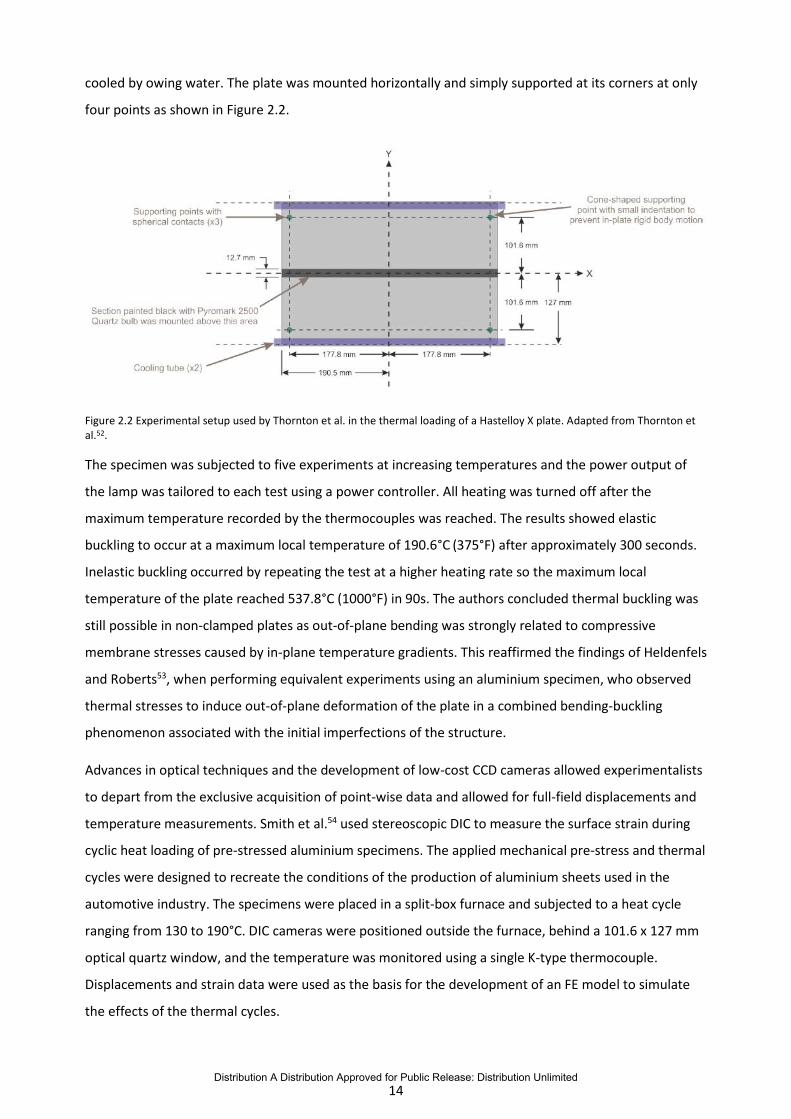
cooled by owing water. The plate was mounted horizontally and simply supported at its corners at only
four points as shown in Figure 2.2.
Figure 2.2 Experimental setup used by Thornton et al. in the thermal loading of a Hastelloy X plate. Adapted from Thornton et al.52.
The specimen was subjected to five experiments at increasing temperatures and the power output of
the lamp was tailored to each test using a power controller. All heating was turned off after the
maximum temperature recorded by the thermocouples was reached. The results showed elastic
buckling to occur at a maximum local temperature of 190.6°C (375°F) after approximately 300 seconds.
Inelastic buckling occurred by repeating the test at a higher heating rate so the maximum local
temperature of the plate reached 537.8°C (1000°F) in 90s. The authors concluded thermal buckling was
still possible in non-clamped plates as out-of-plane bending was strongly related to compressive
membrane stresses caused by in-plane temperature gradients. This reaffirmed the findings of Heldenfels
and Roberts53, when performing equivalent experiments using an aluminium specimen, who observed
thermal stresses to induce out-of-plane deformation of the plate in a combined bending-buckling
phenomenon associated with the initial imperfections of the structure.
Advances in optical techniques and the development of low-cost CCD cameras allowed experimentalists
to depart from the exclusive acquisition of point-wise data and allowed for full-field displacements and
temperature measurements. Smith et al.54 used stereoscopic DIC to measure the surface strain during
cyclic heat loading of pre-stressed aluminium specimens. The applied mechanical pre-stress and thermal
cycles were designed to recreate the conditions of the production of aluminium sheets used in the
automotive industry. The specimens were placed in a split-box furnace and subjected to a heat cycle
ranging from 130 to 190°C. DIC cameras were positioned outside the furnace, behind a 101.6 x 127 mm
optical quartz window, and the temperature was monitored using a single K-type thermocouple.
Displacements and strain data were used as the basis for the development of an FE model to simulate
the effects of the thermal cycles.
Distribution A Distribution Approved for Public Release: Distribution Unlimited
15
Jin et al.8 focused on the use of stereo DIC in the investigation of displacements and strains associated
with the thermal buckling of circular composite plates exposed to a uniformly distributed thermal load.
The specimens were made of glass/epoxy fabric pre-preg and simply supported by a titanium ring. The
specimen was heated in a chamber from 30°C to 120°C at two different load rates: 2°C/min and
7°C/min. Images were acquired throughout the thermal loading at 5° increments, resulting in a total of
19 image pairs for analysis. Experimental results were compared to predictions from an FE model
developed in ABAQUS using temperature-independent material properties and including a generic factor
that accounted for geometric imperfections of the plate. This mirrored the model of Lee et al.55 who
studied the effect of initial geometric imperfections on the critical buckling temperature of laminated
composite panels and found a clear relationship between the two: the critical buckling temperature
increased as the imperfection scaling factor decreased. Experimental results from Jin et al.8 showed the
buckling temperature to be strongly dependent on the rate at which the plate was loaded. In fact, the
authors noted that buckling occurred when applying a 7°C/min thermal load rate, but not when using a
2°C/min heating. The buckling temperature was experimentally determined by analysing the
temperature-displacement relation at the centre of the plate and the DIC displacement map
corresponding to the buckling shape. A very similar methodology was used by Yuan et al.56 to
experimentally determine the buckling temperature and buckled shape of a sandwich panel with a
stainless steel truss core. The square specimen was heated in a furnace where it was horizontally
clamped using a cast iron frame; a stereoscopic DIC system was used to monitor the displacements of
the panel during heating. The cameras were positioned outside the furnace and a view to the specimen
was provided through a double layer quartz glass window. Temperature data was acquired using
thermocouples fitted to the centre and two opposite corners of the specimen. Results from numerical
and theoretical models were found to over-predict the buckling temperature of the panel due to the
lack of defects and imperfections, which were not included in the models. DIC results also showed the
buckled shape to strongly depend on these imperfections as some local yielding was witnessed and not
predicted analytically.
Pan et al.57 also focused on composite structures when studying the thermally-induced out-of-plane
deflection in honeycomb sandwich panels used for thermal protection in hypersonic flight. Their thick,
multi-material sandwich panels were placed in the vertical plane standing on an edge without any
fixation and heated using infrared radiation on one side. A stereoscopic DIC system was used to acquire
displacement data and thermocouples were attached to the front and back surfaces of the panel. The
authors concluded that the maximum deflections of the panel were dependent on the through-
thickness temperature gradient at each point of the loading. Their results showed maximum deflections
were achieved at the same time as this gradient was at its highest value.
Recently, there have been some attempts at the combined acquisition of full-field displacement and
temperature, namely in the study of mechanical energy and heat sources developed locally during
Distribution A Distribution Approved for Public Release: Distribution Unlimited
16
tensile load58, in the investigation of the yield behaviour of semi-crystalline polymers59 and in biomedical
applications for the diagnosis and follow-up of diabetic foot disease60. Orteu et al.33 have published a
journal article describing the use of a single CCD camera for the acquisition of both displacements and
temperatures by performing a radiometric and geometric calibration of the device. The main limitation
of this technique is the amount of preparatory work needed before experiments are conducted and the
temperatures it can measure (values above 300°C).
2.3.1 Conclusions
It is possible to conclude from the above literature review that past work has focused on the
experimental determination of the buckling temperature of simply-supported and fully-clamped plates.
Several findings from these studies are highlighted below:
Compressive stresses due to high in-plane temperature gradients were found to be sufficient to
thermally buckle thin, unclamped plates;
Maximum out-of-plane deflections of a thick, composite panel were shown to depend on the
temperature gradients across its thickness;
Several authors noted that structural imperfections strongly influence the out-of-plane
deflections of thermally-stressed plates; and
A limited number of investigations in the field have used full-field displacement acquisition
techniques and no examples of full-field temperature measurements have been found.
2.4 Analysis and comparison of full-field datasets
Studies presented in 8, 61, 62 aimed to establish a degree of correlation between displacement and
temperature. However, the relationship between experimentally acquired datasets has been limited to
point-based comparisons, either due to practical limitations of the experimental methodology (single
point readings provided by strain gauges and thermocouples), and/or the difficulty in comparing full-
field datasets which do not share the same scale or physical units. This may lead to an under-sampling of
pertinent findings and, therefore, oversimplification of the physical phenomena. However, the increase
in the volume of data acquired when using current optical techniques that provide full-field
measurements poses a new challenge: to distil the significant information and extract relevant
conclusions. Recent developments on the field of FE model validation have proposed a quantitative
methodology for the validation and updating of computational solid mechanics models using
experimental full-field displacement or strain data63-65. At its core, this work involves the comparison of
two datasets - FE predictions and experimental data. On a point-by-point basis, these are data-rich
analyses with extensive data maps that require substantial processing. The authors proposed a data-
fitting method based on orthogonal decomposition that allows for the reduction of comparable two-
dimensional data from thousands of data points to a set of terms. The 2D monomials used as kernel
Distribution A Distribution Approved for Public Release: Distribution Unlimited
17
functions in this polynomial fit are usually known as geometric moment descriptors (GMD)66 or, simply,
shape descriptors (SD)67. The choice of polynomial depends on the data to be represented and several
different studies have been conducted on this topic. The basis of this work prompted the development
of standard directives for the validation of computational models which were published by the Comité
Européen de Normalisation (CEN)68. Wang and Mottershead67 have provided a thorough breakdown on
the advantages and disadvantages of the multiple polynomials used in orthogonal decomposition for
continuous and discrete data.
Teague69 was the first to use continuous Zernike and Legendre polynomials to form shape descriptors
used in the decomposition of data. The fundamental difference between the two was the domain in
which they were defined as Zernike descriptors are orthogonal within a unit circle (therefore, invariant
to rotation of coordinates), while the Legendre polynomials are defined on a rectangular coordinate
system. Wang et al.70 applied orthogonal decomposition using Zernike descriptors as a tool for the
recognition of vibration mode shapes from full-field DIC data. Patki and Patterson71 proposed a hybrid
Fourier-Zernike descriptor to overcome several shortcomings found when using the two descriptors
separately. Whilst the Fourier descriptor did not yield a significant data compression, Zernike presented
limitations in the description of images with discontinuities from geometric features such as holes and
cut-outs. Wang et al.63 attempted to resolve this issue by modifying the Zernike descriptor using a Gram-
Schmidt orthonormalisation of the polynomials over a non-circular domain. The modified descriptor was
then used to compare experimental and computational data pertaining to the measured strain map for
a uniaxially-loaded rectangular plate with a circular hole. However, this method was bespoke to a
specific geometry and would result in a costly process when applied to multiple geometric
discontinuities. One such example is the work proposed by Wang et al.72 and Burguete et al.65 in the
analysis of the dynamic response of geometrically-complex structures under mechanical excitation. The
authors used an adaptive geometric moment descriptor (AGMD) determined by projecting the transient
responses of a car bonnet onto a two-dimensional orthonormal space obtained by mapping the 3D
surface of the structure onto a planar domain. Nevertheless, the discretisation of Zernike/Legendre
polynomials into shape descriptors inevitably introduces numerical errors in the decomposition process.
According to Wang et al.63, the use of discrete Chebyshev (or Tchebichef), Krawtchouk or Hahn
polynomials4 has been proposed to reduce these errors in the evaluation of digital images73-75.
Mukundan et al.73 introduced discrete Chebyshev polynomials as descriptors in image analysis as a
method to extract global features from a dataset, i.e. no specific emphasis is given to a particular
portion or region of the image. Local features, such as edges and other high-contrast areas, were found
to be better represented by Krawtchouk descriptors74. Both Chebyshev and Krawtchouk descriptors are
particular cases of Hahn descriptors75, depending on the parametric definition of the more generalised
polynomial. Non-uniform lattices may also be described by other discrete polynomials, such as the
Racah and the dual Hahn polynomials67. Chebyshev descriptors are of special interest in the analysis of
Distribution A Distribution Approved for Public Release: Distribution Unlimited
18
full-field optical data, as they are defined in a Cartesian coordinate space that better relates to the
regular grid of a pixel array. Wang et al.76 showed the full-field vibration mode shapes of a rectangular
plate with 103 - 104 data points to be effectively represented using 100 - 101 shape descriptors, which
depicts an efficient compression of full-field data. This is because the 2D shapes described by the
discrete Chebyshev polynomials coincide with the mode shapes of an ideal free-free rectangular plate.
The authors used Chebyshev polynomials to decompose and compare experimentally-acquired mode
shapes using DIC and FE predictions. Sebastian et al.77 used a similar method in the comparison of
experimental and computational strain maps of a composite panel under uniaxial compression. A new
procedure for the use of image decomposition as a tool in the validation of FE models was developed
and proposed by Sebastian et al.64 in 2013. In this work, the comparison of full-field displacement and
strain maps from computational models and experiments was shown to be performed effectively using
shape descriptors. The authors deemed validation to be achieved when the coordinate pairs of shape
descriptors from the decomposition of experimental and predictive data lie within a scatter band
defined by the measurement uncertainty. By following this procedure and the protocol established by
the CEN guide68, Berke et al.10 used Chebyshev shape descriptors to validate predictions from their
computational model against mode shape data acquired using DIC. A recent investigation into the use of
Principal Component Analysis (PCA) for the description of full-field experimental results showed this
technique to be a powerful tool in the compression of data (K. Dvurecenska, personal communication,
November 13, 2018)78. This is achieved by a rotation of the axes of the original variable coordinate
system to new orthogonal axes, also known as principal axes, such that the new axes coincide with
directions of maximum variation of the original observations79. However, the study showed the resulting
vectors from the analysis to be difficult to interpret due to the lack of consistent shape descriptors to be
used as reference. Extracting a physical meaning behind the compressed data without that reference
was found impractical.
2.4.1 Conclusions
Orthogonal decomposition has been shown to be a powerful tool to distil the essentials of a data field. A
number of authors found the use of shape descriptors as a basis for fitting of two-dimensional data to
assist in the identification of gradients and patterns across datasets, regardless of the scale and physical
domain in which they occur. The current state-of-the-art evidences a wide range of applications in which
orthogonal decomposition has been used; from validation of predictive models to the identification of
mode shapes acquired experimentally. The choice of descriptor used in data decomposition is based on
the type of data to be analysed, shape of the original datasets and whether the polynomial is to
represent global or local features.
2.5 Knowledge Gaps
Distribution A Distribution Approved for Public Release: Distribution Unlimited
19
From the conclusions sections in the above review, it was possible to identify the following gaps in past
research:
1. From section 2.1, knowledge gap number one: There has been a lack of integration of
structural and temperature data in the developed analytical and numerical models, which has
led to unrealistic predictions. This highlights the need for the development of a finite element
model capable of predicting resonant frequencies and mode shapes for a plate under non-
uniform thermal loading using temperature-dependent material properties and a realistic
geometric representation of the initial curvature of the structure.
2. From section 2.2, knowledge gap number two: No examples of concurrent full-field acquisition
of displacement and temperature have been found when studying the modal response of panel
structures. Whilst Istenes et al50 used a radiometer to confirm uniform temperature
distributions across their specimens, there has been no experimental modal analysis at high
temperatures with full-field thermal mapping. This is likely the reason behind the deficiency in
information on the effect of different non-uniform temperature distributions of the resonant
behaviour of panels. The present project aimed to perform such a study using a commercially-
available thermal camera.
3. From section 2.3, knowledge gap number three: Thin plates have been shown to buckle under
thermal load due to high in-plane temperature gradients. Experiments have been conducted on
isotropic, simply-supported plates and functionally-graded panels using various boundary
conditions and temperature ranges. However, there is a lack of experimental data describing the
behaviour of geometrically-reinforced isotropic plates under thermal load. The literature
includes some examples of full-field displacement measurements but none coupled with full-
field temperature monitoring. Similarly, no studies have been found on the effect of
temperature distribution on thermally loaded panels. An attempt to bridge these gaps is
presented in this thesis.
4. From sections 2.3 and 2.4, knowledge gap number four: The current state of the art shows that
correlations between temperature and displacement measurements have been established in a
point-wise domain. The present thesis proposes the use of orthogonal decomposition to analyse
full-field results and contribute towards an efficient use of experimental data in the validation of
predictive models. The literature shows this technique is yet to be used in the comparison of
data fields with different physical dimensions (i.e. temperature and displacement) and it is
adopted here as a global analysis method applied to multi-physics data.
Distribution A Distribution Approved for Public Release: Distribution Unlimited
Chapter 3 Numerical and experimental methods
This chapter summarises the methods and techniques used in the acquisition and processing of data
presented in this thesis. The first part addresses the numerical methods and overall assumptions used in
the development of a temperature-dependent computational mechanics model. The second and final
part focuses on the experimental methods used to thermally load aerospace-grade metal panels and the
techniques used to measure full-field displacements and temperatures across the specimens.
3.1 Numerical methods
Finite element (FE) modelling has become established as the universally-accepted analysis method in
structural design80. It can be used as a predictive tool capable of solving a wide variety of mechanical,
structural and non-structural problems, including static and dynamic loading, heat transfer and fluid
mechanics. In a general sense, a solution to the FE problem can be achieved in three general steps:
Step 1 - Pre-processing or "defining the problem": construction of a discrete system of individual
elements that represent the mass and stiffness of a continuous structure, known as a mesh. This is
known as a piecewise approximation of a continuous domain. Each element defines a discrete area (in
shell geometries) or volume (for solid geometries) and is defined by a mathematical description,
regardless of the overall geometric complexity of the structure. The boundaries of each element are
defined by a unique polynomial curve or surface that connects the boundary node points between
elements and are used to establish a relation between individual elements and the displacements of the
nodes, in a process called shape function interpolation80. In the pre-processing of an FE analysis, nodes,
elements and boundaries relevant to the structure are defined, along with material properties which will
affect the mathematical description of the elements. Loading conditions are also programmed into the
analysis through the application of a distributed load or pressure, whilst boundary conditions specify
how the structure is constrained. The analyst must also select the type of analysis based on the physical
behaviour of the model. This determines the mathematical model to be used in the solving of the
analysis and the governing equations of the model; it may include, for instance, defining whether the
analysis is linear/non-linear or if it represents a mechanical/thermal/combined loading scenario. The
output of the pre-processor is a set of definitions and instructions that are fed to the solver.
Step 2 – Solving the problem: The FE solver processes the code from the pre-processor using specific
algorithms and provides an output that corresponds to the solutions of the analysis. For the present
work, the chosen solver was LS-DYNA (Livermore Software Technology Corporation, California, USA) as it
is particularly powerful when solving dynamic problems. When processing the instructions from the pre-
processor, the FE solver converts the governing mathematical model into element models by fitting a
set of trial functions into the original governing equations and minimising the error between the two.
Distribution A Distribution Approved for Public Release: Distribution Unlimited
21
For each element, the solver determines three descriptors: 1) element shape functions, 2) element
stiffness matrices (geometric and material stiffness), and 3) element load vectors. The solver then
assembles the mathematical description of every element (either one or a set of partial differential
equations) in a large system of equations that models the entire problem and enforces the continuity of
displacements between element boundaries. This is achieved through a transformation of the element
models from local coordinates systems to a global coordinate system.
When assuming a linear relation between load and displacement, the solver assembles the global
stiffness (K) and force (F) vectors and, for a static analysis, solves the equation:
𝐾𝑈 = 𝐹 (3.1)
where U is the unknown displacement vector.
However, when the global stiffness matrix changes throughout the analysis, the displacement-load
relation becomes non-linear and the same assumption cannot be made. This may occur due to non-
linearities in the displacement-strain relation (geometric non-linearities, e.g. large displacements) or
strain-stress relation (material non-linearities, e.g. plastic deformation). In such cases, the solution to
the above equation becomes:
𝐾𝑈(𝑈) = 𝐹 (3.2)
which requires the recalculation of the global stiffness matrix throughout the loading, as it becomes
dependent on the global state of each element. Current FE software provides the analyst with a choice
on which method to use in the calculation of the displacement vector, U. Given the iterative process
required in the recalculation of the global stiffness matrix, however, non-linear analyses are typically
more time consuming.
Step 3 – Post-processing:
The post-processor decodes the output from the solver and gives the analyst several tools to view the
or tables, etc. HyperWorks (Altair Engineering, Michigan, USA) was used for the pre-processing of
analyses and post-processing of results due to its meshing capabilities and easy interface with LS-DYNA.
The specification of algorithms to be used by the solver in the processing of analyses was selected based
on the requirements of the study. A structural-thermal solution procedure in LS-DYNA was required
when defining temperature-dependent properties in the model. Heat transfer analysis was coupled with
the mechanical solver to calculate the effect of temperature on the structure.
An eigenvalue analysis was used in the investigation of the modal response of the plates to compute the
solution of the equation of motion for the resonant frequencies (eigenvalues) and corresponding
Distribution A Distribution Approved for Public Release: Distribution Unlimited
22
vibration mode shapes (eigenshapes). This method assumes negligible damping and no applied loading,
reducing the equation of motion to the eigenequation:
[𝐾] − 𝜆[𝑀]{𝜙} = 0 (3.3)
where 33 is the stiffness matrix of the component, 70, 81, 82 corresponds to its mass matrix, 𝜆 is the
resonant frequency and {𝜙} is the corresponding mode shape. Alternatively, a modal frequency
response could have been performed by applying a mechanical excitation to a thermally loaded plate
and computing its response. However, this is a time-consuming method that requires a separate
computational analysis to be performed for each resonant frequency and temperature distribution. The
eigenvalue method expedited the acquisition of results by enabling the extraction of resonant
frequencies and mode shapes at different increments of the thermal loading using a single
computational analysis. This allowed for a quasi-continuous monitoring of the modal response of the
structure from room temperature to a high-temperature steady state. The eigensystem solutions were
extracted using the linear iterative Lanczos extraction method, which is standard in most FE packages83;
no damping was modelled.
A double precision executable LS-DYNA solver was used in order to improve accuracy of results as the
single precision executable yielded inconsistent results due to truncation errors in the calculations
associated with the fine mesh applied to the model84.
All analyses were performed using an implicit solver. In implicit analysis, displacements calculated at
each time step are not a function of time so that velocities and accelerations are zero, and mass and
damping factors can be neglected. The time dependency of the solution is not an important factor in
modal analysis, as resonant frequencies and shapes are extracted by solving a static eigenvalue
problem. By using an implicit solver, solutions have been calculated using mathematical iterations to
enforce equilibrium at each time step until a final result is reached. As this is an iterative process which
requires the inversion the stiffness matrix, it is a computationally expensive process. However, this is
often offset by the fact it does not require small time steps unlike explicit methods which define
displacements as a function of time.
3.2 Experimental methods
3.2.1 Infrared heating
Infrared lamps were used to heat the specimens up to maximum temperatures of approximately 700°C
due to their inexpensive and replaceable nature and the ability to easily control their power output to
create different temperature distributions across the panels. In the context of this work, these
advantages greatly outweigh the typical higher energy losses associated with the use of radiant heating
in comparison with induction methods which rely on electric currents induced internally in the material
Distribution A Distribution Approved for Public Release: Distribution Unlimited
23
to be heated85. In induction heating, the flow of AC current through a conductive coil (generally copper)
generates an alternating magnetic field, which induces eddy currents in the specimen. The specimen
behaves like a resistance through which the eddy currents ow generating an increase in temperature
due to resistive (or Joule) heating. Thus, the method strongly relies on the electric conductivity of the
material to be heated, which limits its use when studying non-ferrous specimens.
In the work here presented, halogen quartz lamps with a power output of 1kW each and a colour
temperature of 3210 K were used for heating the specimens (QIR 240 1000 V2D, Ushio, Steinhöring,
Germany). The lamps were mounted in uniformly spaced arrays of six with a reflective back-plate so to
maximise the energy provided to the test specimens. The centre-to-centre distance between lamps was
approximately 3.5 cm. The power output of the lamps was regulated by a controller using TRIAC
semiconductors. The specimens and lamps were not enclosed in a furnace so that there were
substantial heat losses from the apparatus, but the optical access was excellent.
3.2.2 Full-field infrared thermography
The use of optical techniques in the monitoring and measuring of temperatures was expedited in the
early 1900s after the photon effect based on photoconductivity was discovered by W. Smith in 187386.
Two different types of detectors were then developed: photon detectors, and thermal detectors or
bolometers. Photon detectors rely on the principle of photoconductivity as photons of specific
wavelengths are absorbed by the sensor and create free electron-hole pairs, which can be detected as
electrical current. However, the output signal is very small and easily overshadowed by internally-
generated thermal noise in the device, which results in the need for it to be cryogenically cooled. Active
cooling is not required in bolometers, which produce an electrical response based on a change in
temperature of the sensor. The need for thermal equilibrium to be reached within the bolometer
detector after the absorption of radiation (thermalisation) caused them to have a lower sensitivity and
their response time to be considerably slower than photon detectors. However, manufacturing
advancements in the 1970s made it possible to produce smaller, thinner pixel-based thermal detectors
which narrowed the differences between the two technologies86.
In the high-temperature work presented in this thesis, both types of infrared detectors were used.
Initially, a commercially-available photon detector (SC7650E, FLIR, North Billerica, MA, USA) was used to
monitor the temperature distribution on the surface of the specimen. The camera has a focal plane
array of 640 x 512 pixels with a maximum recording rate of 100 frames per second at this resolution and
a typical sensitivity of 20 mK at wavelength from 3 µm to 5 µm. Despite the high sensitivity of the
camera, the system was not calibrated for temperatures above the 150°C, which restricted the
maximum temperatures detected before the sensor saturated. A reflective neutral density (ND) filter
with a usable range between 2 and 16 µm (NDIR20B, Thorlabs Inc., New Jersey, USA) was fitted to the
Distribution A Distribution Approved for Public Release: Distribution Unlimited
24
camera to prevent saturation and a manual calibration was performed with the aid of a laser-guided
infrared thermometer (Fluke 62, Fluke
UK Ltd, Norfolk, UK). This calibration method for the camera was prone to error due to the complicated
process involved; and so, in subsequent experiments a micro-bolometer with an accuracy of ±2 °C or ±2
% (whichever is greater) was used. The commercially-available uncooled micro-bolometer (TIM 400,
MICROEPSILON UK, Birkenhead, UK) was a more economic option in the monitoring of temperatures
than the photon detector. Its 25 µm × 25 µm focal plane array sensor has a 382 x 288 pixel resolution
and a maximum frame rate of 80Hz. The sensor is sensitive to a spectral range of 7:5 µm to 13 µm and a
thermal sensitivity of 0.1K with the chosen telephoto lens (13° x 10° FOV; F = 1.0). The device is factory-
calibrated and includes an automated "ag" system that is periodically positioned in front of the sensor
as a constant temperature reference to reduce the variations in the response of each pixel to the
infrared energy. Using the control software of the micro-bolometer (TIM Connect, MICRO-EPSILON UK,
Birkenhead, UK), this non-uniformity correction was programmed to take place in-between data
acquisition frames to avoid the introduction of erroneous readings if performed when recording data.
The range of temperatures studied bridged two available calibration ranges: 0-250 °C and 150-900 °C;
hence, a compromise was made to use a camera calibrated in the 150-900 °C range with an option
selected that extended the calibration down to room temperature. This resulted in an increase in the
amount of noise for room temperature readings, which decreased the system's accuracy to 5-7 K (worst
case scenario), according to the manufacturer. Since the work presented here is primarily focused on
phenomena at temperatures beyond 150 °C, the higher uncertainty of measurements at lower
temperatures was accepted.
3.2.3 Digital image correlation
Several full-field techniques can be used for the measurement of displacements and strain at high
temperatures. In a broad sense, the methodology spectrum can be divided into two major groups: 1)
interference methods, such as holography or moire interferometry, which make use of coherent light
and, therefore, depend on its wave properties, and 2) other methods that use non-coherent light and
include photoelasticity, digital image correlation (DIC), fringe projection and grid methods. Sebastian11
has provided a detailed breakdown of viable full-field measurement techniques and their inherent
strengths and weaknesses. In the present work, stereoscopic-DIC was used in the acquisition of
displacements and specimen shape data because it is capable of gathering full-field information at a
large range of temperatures, specimen sizes, time scales and loading rates. It is a robust technique with
a relatively simple setup and low sensitivity to unintentional vibration and rigid body movements during
testing; both these factors contribute towards it being an attractive method to be used in industrial
settings. Despite requiring very simple specimen preparation using readily available temperature-
resistant materials, this technique provides a rich data set by being capable of measuring in-plane and
Distribution A Distribution Approved for Public Release: Distribution Unlimited
25
out-of-plane displacements, as well as object shape. DIC uses digital images of an object or structure at
difference stages of deformation and employs tracking techniques to measure surface displacement and
build full-field 2-D and 3-D displacement fields and estimated stain maps. 2-D DIC is the simplest
example of this method, as a single camera is used in the acquisition of images and only in-plane
deformation can be measured. Stereoscopic-DIC (or 3D-DIC) uses two cameras to acquire image pairs at
each deformation stage, which introduces the ability to trace out-of-plane displacements and provide
data pertaining to the curvature of the object through point triangulation. It is also possible to perform
stereoscopic-DIC with a single camera using additional optical devices like diffraction grating, a bi-prism
or a set of planar mirrors, which are used to record pseudo images of the imaged object87.
Experimentalists have also successfully used systems of multiple cameras (2+) to acquire groups of
images per deformation stage, which was shown to be an effective way to enlarge the measurement
field without losing effective resolution in the area of interest88-91.
In DIC, each digital image is an effective intensity array which is divided into overlapping, square subsets,
called facets. The size of these subsets is based on the spatial frequency of the pattern being imaged to
ensure each facet is unique and the DIC system cannot mistakenly identify it as a different facet. For this
purpose, Sutton et al.92 recommended that an optimised facet should contain at least nine uniformly
distributed speckles. Prior to loading, an image of the object or structure is acquired and defined as the
reference image. Subsequent images are acquired at different stages of loading and are termed
deformed images. Image correlation is performed by comparing the facets from the reference image to
the facets from each of the deformed images using a correlation algorithm based on image matching. A
point within a facet of the reference image, 𝑃(𝑥, 𝑦) can be mapped to a point in a facet of each of the
deformed images, 𝑃∗(��, ��) using the displacement components u and v in Equations 3.4.
�� = 𝑥 + 𝑢(𝑥, 𝑦)
�� = 𝑦 + 𝑣(𝑥, 𝑦)
(3.4)
A schematic of the image correlation process applied to 2D-DIC is shown in Figure 3.1, where point 𝑃1 in
the reference image is matched to point 𝑃1∗
in the deformed image. The shape of the deformed facet is
modelled using a high order shape function that transforms pixel coordinates in the reference facet into
coordinates in the image after deformation92. In the work here presented, the DIC software used a
second-order function (shape function) to locate and map each subset to its distorted shape93, as
defined by the following equations:
Distribution A Distribution Approved for Public Release: Distribution Unlimited
26
�� = 𝑥0 + 𝑢0 +
𝜕𝑢
𝜕𝑥𝛥𝑥 +
𝜕𝑢
𝜕𝑦𝛥𝑦 +
𝜕2𝑢
𝜕𝑥𝜕𝑦𝛥𝑥𝛥𝑦
�� = 𝑦0 + 𝑣0 +𝜕𝑣
𝜕𝑥𝛥𝑥 +
𝜕𝑣
𝜕𝑦𝛥𝑦 +
𝜕2𝑣
𝜕𝑥𝜕𝑦𝛥𝑥𝛥𝑦
(3.5)
where (𝑥0, 𝑦0) and (��, ��) represent the coordinates of the centre of the facet in the reference and
deformed image, respectively. The in-plane displacements are defined by 𝑢0 and 𝑣0, whilst the
remaining parameters in the shape function define surface slopes and distortion. The terms in Equation
3.5 are determined using a sum of squares deviation to minimise the differences between the reference
and deformed facets.
Figure 3.1 Schematic representation of the DIC process in which an undeformed facet in the reference image is mapped onto a deformed facet in an image acquired post-loading.
The deformation of the object or structure introduce non-integer displacements of the corresponding
positions in the reference image94, which requires the discrete, pixel-based intensity values of the
deformed images to be interpolated and converted into a continuous functional representation of the
original images. This allows for displacements to be determined to a sub-pixel accuracy. Different
interpolation methods may be used in this process. Figure 3.2 a) shows an example of a 16 x 16 pixel
greyscale image which was then plotted in Figure 3.2 b) to illustrate the discrete intensity values at each
pixel that range from 0 (black) to 255 (white). A bi-linear interpolation of the original pixel map is shown
in Figure 3.2 c) and represents a computationally efficient option but at a cost: a large bias, particularly
when processing noisy images95. In the work presented in this thesis, a bi-cubic spline was used to
acquire sub-pixel accuracy of displacements, which is exemplified in Figure 3.2 d). Whilst
computationally more expensive, investigations by Bornert et al.95 and Sutton et al.92 shows the bi-cubic
spline to yield the lowest bias error and the lowest random error when compared to other typically used
methods such as bilinear and bi-cubic polynomial interpolation. According to Bornert et al.95,
Distribution A Distribution Approved for Public Release: Distribution Unlimited
27
interpolation using an optimised bi-cubic spline filter can result in a bias of approximately 1:1 x 10⁻³
pixels for noiseless images and 13 x 10-3 pixels for images with added noise.
Figure 3.2 Discrete grey level representation of intensity values for a 16 x 16 pixel array. Image credit. The b) Three-dimensional, c) bi-linear and d) bi-cubic spline representations of the same pixel array are included.
2D-DIC requires the calibration of the system so that a total of eleven independent parameter are
determined: six extrinsic parameters that describe the orientation and position of the camera, and five
intrinsic parameters which define the imaging parameters for the camera93. This is achieved by acquiring
several images of a known target that undergoes arbitrary motion. In the calibration process, the DIC
software effectively estimates the transfer function of the DIC system by recognising a pattern in the
acquired images of the calibration target (fiducial points) and analysing it against known characteristics
of that pattern. In a stereoscopic rig, both cameras acquire images of the object or structure at the same
stage of deformation and, as such, they must share a common coordinate system. An equivalent
calibration process to the one described for 2D-DIC is applied to determine the intrinsic parameters for
each camera and the relative positions and orientations of the cameras with respect to each other93.
When calculating the deformations experienced by an object or structure under load, these parameters
are used to calculate the 3D position of each surface point and provide both in-plane and out-of-plane
displacement data. According to Sutton94, the typical accuracy of these measurements is in the order of
Distribution A Distribution Approved for Public Release: Distribution Unlimited
28
±1/100 pixels and for in-plane displacement components and ±Z/50000 for out-of-plane displacement
components, where Z is the distance from the cameras to the object or structure.
Another advantage of stereoscopic DIC compared to its 2D counterpart is its ability to provide
information about the shape of the imaged object or structure. The DIC software selects the subsets in
the reference image, acquired using the master camera, and performs image correlation to locate the
matching positions in the image acquired using the second camera. The intrinsic and extrinsic
parameters calculated during the calibration of the DIC system are then used to determine the optimal
three-dimensional position of the common object point for each matching pair of subsets, which results
in a dense set of three-dimensional points that represent the shape of the object. Figure 3.3 shows a
schematic of the stereoscopic DIC process when tracking a point 𝑃, which represents the centre of the
highlighted facet.
Figure 3.3 Schematic representation of the typical stereoscopic-DIC process.
In the work presented in this thesis, a commercially-available stereoscopic DIC system was used (Q-400
system, Dantec Dynamics GmbH, Ulm, Germany), which consisted of two 1624x1234 pixel CCD Firewire
cameras (2MP Stingray F-201b, Allied Vision Technologies GmbH, Stradtroda, Germany) _fitted with a
set of 12 mm lenses (Cinegon, 1.4/12, Schneider). The maximum frame rate of the cameras was 14
frames per second at full resolution.
Distribution A Distribution Approved for Public Release: Distribution Unlimited
29
The surfaces of specimens are prepared for DIC measurements by applying a high-contrast random
pattern to the regions of interest; this is fundamental in the characterisation of facet position and
displacement tracking. Whilst DIC has been performed using many types of object-based patterns, such
as lines, grids, dots, random arrays and features, the most commonly used method is the use of random
speckle patterns achieved using high-contrast paints. In this work, specimens were prepared for high
temperature measurements using DIC by spraying them with a uniform layer of commercially-available
refractory black paint (VHT Flameproof, Cleveland, Ohio, USA). A white version of the same paint was
used to create a speckle pattern. The more usual reverse colour scheme was considered but disregarded
because the black background used here enables a larger transfer of radiation and results in higher
specimen temperatures. The scale of the region of interest determined the process used for the creation
of the speckle. A large speckle size requires the use of a large subset that can approximately
accommodate the nine, uniformly-distributed speckles recommended by Sutton92; however, this
compromises spatial resolution. A speckle size that is too small increases the noise level in the results
and the risk of aliasing. Multiple optimal speckle sizes have been recommended in literature but the
most generally accepted convention is approximately 3-5 pixels in diameter92, 96. The misting or spraying
of the base colour with a contrasting paint is typically a good method for the generation of small, dense
speckle patterns. In the present work, however, a suitable speckle size could not be achieved using spray
nozzles as the full-field view of the specimen rendered the resulting speckle to be greatly below the
conventionally accepted size. Promising results were achieved using a short bristle brush, which was
slightly distressed, and lightly dipped in paint and flicked onto the specimen; however, there was a
directionality to the speckle due to the momentum of the paint droplets. This directionality is
undesirable as oriented features limit the determination of motion vector components which are
orthogonal to the object or structure92. Qualitatively, the most even speckle distribution was achieved
by using a 1 inch (2.54 mm) wide brush dipped in paint and held horizontally, approximately 20 cm
above a horizontal specimen. By firmly tapping it, the resulting speckle was achieved by force of gravity
and lateral deviations to the droplet trajectories were kept to a minimum. Fiji by ImageJ97, 98 was used to
analyse a high-quality image of the speckled specimens acquired using one of the CCD cameras: a
threshold equal to the mean grey level across the plate was defined and the particle analysis tool
available in the software was used to calculate the average speckle size. This was found to be around 14
pixels2, which corresponds to an average speckle diameter of approximately 4 pixels when assuming a
perfectly circular shape. Images of the resultant speckle pattern can be found in Chapters 5 and 6,
where the experimental results of this work are documented.
Compared to its room temperature counterpart, there are several added challenges when performing
DIC at high temperatures. The most common problem is the increased in black body radiation. The most
common problem is the increase in black body radiation. Whilst, in the past, traditional DIC methods
without any special optical setup have been used successfully up to approximately 600°C99, radiation
Distribution A Distribution Approved for Public Release: Distribution Unlimited
30
from the test specimen becomes visible to the naked eye when its temperature goes beyond 1000K
(727°C). However, most CCD camera sensors are sensitive to radiation emitted by bodies below this
temperature, which interferes with the imaging process by altering the contrast between surface
features and often saturates the camera sensors. Several researchers have shown that undesired
radiation from high-temperature experiments can be eliminated by the use of narrow band lighting and,
or optical bandpass filters 10, 11, 100-103. Experimental displacement data presented in this thesis was
acquired using stroboscopic illumination of the specimen provided by a pulsed-laser with a wavelength
corresponding to the peak quantum efficiency of the CCD sensors in the DIC cameras. This consisted of
an Nd:YAG laser (Nano L200-10, Litron, Rugby, England) that emitted a 4-nanosecond pulse of green
light (532 nm) which was expanded after passing through a spatial _lter2 to produce a speckle-free beam
of approximately 1 m in diameter. The laser was placed directly in front of a specimen, providing it with
uniform illumination and granting equal exposure for the images captured by both cameras. Optical
bandpass filters with a centre wavelength of 532 nm and 4nm bandwidth were fitted to the standard
DIC cameras in order to block any light outside of the wavelength of the laser. Simultaneous triggering
of the laser pulse and DIC image acquisition was achieved by connecting both systems to a timing box.
The deterioration or oxidation of the paint at high temperatures is another challenge to overcome, as it
tends to volatilise with the increase in temperature. Researchers have applied very sophisticated
methodologies to solve this problem at temperatures above 1000°C, from the airbrushing of alumina
and zirconia paints101, to the use of plasma spray to speckle tungsten powder onto carbon composites62.
Commercially-available, temperature-resistant paint has been shown to withstand temperatures of
about 600°C without any significant degradation in the accuracy of the measurements99. However,
Sebastian11 experienced some problems with the flaking and discolouration of temperature-resistant
paint at equivalent temperatures. So to prevent this from happening in the experiments described here,
P120 sandpaper was used to lightly score the surface of the specimens before the black VHT Flameproof
base paint was applied; this was done in accordance to the directions of the paint manufacturer and no
flaking of the paint was witnessed. No visible discolouration was witnessed at the temperature range
studied in this thesis (from room temperature to just below 700°C), which was confirmed by Berke et
al.103 who found this particular paint to discolour at temperatures on the order of 750°C.
The final issue identified by researchers when performing high temperature DIC was the role of a heat
haze in the distortion of results. This is typically induced by the transient variations of the refractive
index of the heated air104 when the air temperature between the cameras and the specimen being
imaged is not homogeneous. Unfortunately, the influence of the heat haze in DIC measurements is not
yet well-understood as it heavily depends on the experimental setup used in each study105. However,
Pan et al.104 have showed the influence of the heat haze to be negligible when positioning the specimen
vertical and perpendicular to the optical axis of the imaging system. In the experiments presented here,
that configuration was adopted. The distance between the cameras and the specimen was also kept to a
Distribution A Distribution Approved for Public Release: Distribution Unlimited
31
necessary safe minimum, as large distances between the specimen and cameras promote the formation
of a heat haze. To facilitate the mixing of the air around the experimental setup, tests were performed
in a ventilated room with an extractor fan, as recommended by Lyons et al.106.
Figure 3.4 Photograph of the setup used in the experiments performed as part of this project.
In each experimental chapter of this thesis, a detailed schematic of the setup is presented, however,
Figure 3.4 shows an overview of the rig used in the experimental work performed as a part of this
project. Note the DIC-ready specimen included in the photograph and mounted in front of the quartz
lamps.
Distribution A Distribution Approved for Public Release: Distribution Unlimited
Chapter 4 Development of a temperature-dependent material
model using finite element analysis
4.1 Introduction
One objective of this project focused on the development of a Finite Element (FE) model, with
temperature-dependent material properties, to be used as a tool capable of accurately predicting
resonant frequencies and mode shapes of a thin plate subjected to elevated temperatures and at
different stages of the thermal loading.
In this development chapter, an in-depth description of the model is provided and each assumption is
explained. Results are presented and compared to experimental and predictive data published in 2015
by Berke et al.10 as a way to build on previous modelling work undertaken by the research group. This
previous model assumed small strain linear elastic response with no thermal expansion or conduction
modelled. As explained in section 2.1, Berke et al. introduced a temperature-dependent Young's
modulus by assigning specific values to the nodes affected by a discrete temperature distribution
divided into 6 levels. This temperature distribution was computed from stereo-DIC strain data and
material data provided by the manufacturer107. The analysis was defined as a static event with no
dynamic increase in temperature having been programmed into the model. Their frequency predictions
yielded no significant changes in resonant frequency with temperature, which was not confirmed
experimentally. There were several possible causes for this disparity of results: 1) the use of an overly
simplistic material model; 2) not capturing thermal stresses accurately when performing a static analysis
using FE; 3) poor depiction of the temperature changes during the oscillation period. Whilst the latter
can only be experimentally tested, a systematic study was undertaken to identify which parameter or
number of parameters were responsible for the shortcomings of this past model. Results were also
compared to predictions from Bailey26, 27, Jeyeraj et al.33 and Murphy et al.44 on thermally stressed plates
in an attempt to establish a framework for further developments that are presented in Chapter 5 and
involved the integration of experimentally-acquired geometric data (out-of-plane curvature of the plate)
and temperature data in the model. Hence, it was critical to develop a robust, reliable model that could
not only be used to recreate the conditions of future experimental work, but could help in the design
the experimental setup, techniques and protocols.
The structure of this chapter deviates from that of the subsequent results chapters because it describes
an iterative development process of a computational model; thus, the results of the multiple separate
studies are presented before an overall discussion and consequent conclusions are drawn in the context
Distribution A Distribution Approved for Public Release: Distribution Unlimited
33
of this project. This chapter is based on the following conference paper, presented at the British Society
for Strain Measurement 12th International Conference on Advances in Experimental Mechanics:
A. C. Santos Silva, C. M. Sebastian, E. A. Patterson, "Acoustic response of thermally stressed plates using
a temperature dependent finite element material model", BSSM 12th International Conference on
Advances in Experimental Mechanics, 2017.
4.2 Definition of a temperature-dependent material model applied to a
static loading analysis
An initial attempt at a predictive model with temperature-dependent material properties aimed to
computationally recreate the laboratory conditions described by Berke et al.10. The resulting model was
then used to study the first hypothesis proposed by these authors to explain the discrepancies between
their experimental results and FE predictions: an overly simplistic material model. Consequently, the
focus was not on the computation of thermal stresses but on the development of the material model
itself and its application to a plate under constant load (static analysis). The specimen studied was a at
120 x 80 x 1.016 mm Hastelloy X (Haynes International, Kokomo, IN USA) plate modelled in Hyperworks
(Altair Engineering, Michigan, USA) using 1 x 1 mm quadrilateral shell elements (9801 nodes in total,
akin to Berke et al.'s FE model). These elements were applicable due to the specimen being assumed to
be a Kirchhoff-Love plate (thin plate) which can be fully described in two-dimensional form using its mid-
surface plane. The recommended shell formulation for implicit analyses in LS-DYNA was selected (type
16 - fully integrated with 4 in-plane and 5 through-thickness integration points)108, as it uses a "local
element coordinate system that rotates with the material to account for rigid body motion"109 and avoid
element locking phenomena1. The plate was modelled in the x – y plane with out-of-plane
displacements in the z-direction. A single central node (x,y) = (0, 0) was completely restrained (zero
degrees of freedom). It is important to stress that, at this point in the study and unlike the work from
Berke et al., this geometry was assumed to be an ideally at plate and did not account for geometric
imperfections.
The values of temperature-dependent material properties of a Hastelloy X plate were provided by the
manufacturer107 and integrated into an isotropic thermal material model available in LS-DYNA (MAT
ELASTIC PLASTIC THERMAL) by defining property curves that described how the Young's modulus, mean
coefficient of thermal expansion, thermal conductivity and heat capacity changed with temperature.
These curves have been plotted and are available in Appendix A. The Poisson's ratio of the material was
assumed to be constant as values provided by the manufacturer showed this parameter not to be
significantly affected by temperature. The material was assumed to have an elastic response and a
constant mass density at 8220kg/m3. Despite the fact that metal plates are often manufactured using a
rolling process that induces a directionality to the grain orientation, the material was assumed isotropic
Distribution A Distribution Approved for Public Release: Distribution Unlimited
34
for simplicity and because that level of material data can be difficult to acquire for existing aircraft
structures.
Figure 4.1 Experimental temperature distribution estimated by Berke et al.10 (left) and the recreated map using the developed MATLAB script (right).
The analysis was defined assuming a linear relation between load and displacement and the stiffness
matrix was assumed constant throughout the study. A uniform room temperature (22°) was applied to
the plate and the first nine eigenvalues and eigenshapes were extracted. The process was repeated at
higher temperatures using an equivalent temperature distribution to Berke et al. A MATLAB script was
written to replicate the discrete temperature distribution used by the authors and assign the correct
temperature values to the FE nodes shown in Figure 4.1. The original image on the left of Figure 4.1 was
converted to greyscale and its intensity values divided into six discrete levels. Then, each of these levels
was assigned a temperature value that reproduced the distribution used by Berke et al. in their
simulation work. Any discontinuities in the data map in Figure 4.1 (left) were interpolated using
MATLAB's default nearest neighbour function.
The combination of static loading, a flat geometry and a fine mesh prevented hourglassing from
occurring and so no correction was necessary. Studies on the impact of gravity loading on the modal
response plate were undertaken and no effect was witnessed. The developed static model with
temperature-dependent material properties was then used to perform two simple investigations that
aimed to improve predictions. The first investigation was conducted to understand how the FE
predictions would be affected by the simplification of the material model due to the lack of mechanical
and, or thermal performance data. A first degree polynomial was used to interpolate the temperature-
dependent Young's modulus, mean coefficient of thermal expansion and thermal conductivity; the
resulting curves are shown in Figure B.1 of Appendix B. Heat capacity and Poisson's ratio remained
unchanged. Predictions using the original and simplified material models (FS) were compared to the
experimentally-acquired frequencies published by Berke et al. (FE) by calculating the relative error of the
FE results as:
𝑅𝑒𝑙𝑎𝑡𝑖𝑣𝑒 𝑒𝑟𝑟𝑜𝑟 =
|𝐹𝐸 − 𝐹𝑆|
𝐹𝐸 × 100% (4.1)
Distribution A Distribution Approved for Public Release: Distribution Unlimited
35
Figure 4.2 Constrained nodes studied for the uniform plate. All permutations were centred on the plate's central node: (x, y) = (0, 0).
Figure 4.3 Constrained nodes studied for the plate with a hole. All circular constraints were centred on the plate's central node: (x; y) = (0; 0).
Results from this study are also presented in Appendix B. Room temperature frequency predictions did
not present any significant change with the simplification of the material model. High temperature
predictions were seen to be only marginally more sensitive to this simplification, as their mean relative
error increased by 0.1% when using the fitted material model. Regardless, the difference in relative
error against experimental data for all resonant frequencies predictions using the original and simplified
models was below 0.6%, which demonstrated a good agreement of results. Hence, the model was found
to be robust to variations in the temperature-dependent material properties that might occur when a
limited amount of material data is available to the analyst. The original material data provided by the
manufacturer107 was used in all analyses on Hastelloy X components presented in this thesis.
The second investigation aimed to identify which boundary conditions best replicate Berke et al.'s
experimental setup and various permutations of fully-constrained nodes were analysed. The developed
static model previously described in this chapter was used and a spatially uniform room temperature
distribution was applied. Predictions using different patterns of nodal constraints were compared to the
experimental results from Berke et al. All of the patterns were centred on the central node of the plate:
(x, y) = (0, 0). Figure 4.2 depicts the different types of nodal constraints applied to the flat plate. The
hexagonal constraint aimed to replicate the nut attaching the plate to the stinger in the experimental
setup.
Distribution A Distribution Approved for Public Release: Distribution Unlimited
36
The geometry used in the static FE analysis was then substituted by a flat plate with a 5 mm circular hole
modelled at its centre. This aimed to better replicate the plate used in the DIC experiments performed
by Berke et al. which included a hole through which a stinger was attached. Figure 4.3 illustrates the
different fully constrained nodal patterns on the plate with a hole.
Comparing the resonant frequency results of each iteration against experimental data, the minimum
relative error computed was found for the single, central constraint type, which was then used in the
subsequent studies. Evidence of this study is available in Appendix C.
4.2.1 Results
Figure 4.4 shows three data sets pertaining to the first nine mode shapes of the 120 x 80 x 1.016 mm
Hastelloy X plate at room temperature; no hole was modelled in the plate which was fully constrained
about its single central node. Whilst Figure 4.4 a) and b) show the experimental and predicted results
published by Berke et al., respectively, Figure 4.4 c) includes predictions from the developed static
model with temperature-dependent material properties.
Qualitatively, Figure 4.4 shows that both the current static model and Berke et al.'s model depict the
shapes of the plate's first nine natural modes accurately at room temperature. As experimental
displacements heavily depend on the amplitude of the excitation signal, the analysis was focused
around the overall shape of each mode (relative displacements) instead of the absolute magnitude of
displacements. Similarly, high temperature results relative to the temperature distribution in Figure 4.1
are shown in Figure 4.5.
Resulting resonant frequencies were compared with the DIC experimental data tabulated by Berke et al.
in 10, which was taken as reference, and relative errors calculated. This comparison was made at a
uniform temperature of 22°C and at higher temperatures distributed according to Figure 4.1. The
average relative error of both analyses can be found in Table 4.1. A more comprehensible comparison of
resonant frequencies results is available in Figure 4.6.
Table 4.1 Mean relative error of Berke et al.'s10 FE model and the current static model against experimental data.
Distribution A Distribution Approved for Public Release: Distribution Unlimited
37
Figu
re 4
.4 M
od
e sh
apes
re
sult
s o
f a
12
0 x
80
x 1
.01
6 m
m H
aste
lloy
X p
late
at
roo
m t
emp
erat
ure
, wh
ich
incl
ud
e a)
exp
erim
enta
l res
ult
s ad
apte
d f
rom
Ber
ke e
t al
. 10, b
) p
red
icti
on
s fr
om
th
e
mo
del
dev
elo
ped
by
Ber
ke e
t al
. 10
, an
d c
) p
red
icti
on
s fr
om
th
e cu
rren
t te
mp
erat
ure
-dep
end
ent
FE m
od
el w
ith
sta
tic
load
ing.
Distribution A Distribution Approved for Public Release: Distribution Unlimited
38
Figu
re 4
.5 M
od
e sh
apes
re
sult
s o
f a
12
0 x
80
x 1
.01
6 m
m H
aste
lloy
X p
late
at
the
tem
per
atu
re d
istr
ibu
tio
n in
Fig
ure
4.1
, wh
ich
incl
ud
e a
) ex
per
imen
tal r
esu
lts
adap
ted
fro
m B
erke
et
al. ,
b)
pre
dic
tio
ns
fro
m t
he
mo
del
dev
elo
ped
by
Ber
ke e
t al
.10 , a
nd
c)
pre
dic
tio
ns
fro
m t
he
curr
ent
tem
per
atu
re-d
epe
nd
en
t FE
mo
del
wit
h s
tati
c lo
adin
g.
Distribution A Distribution Approved for Public Release: Distribution Unlimited
39
Figure 4.6 Resonant frequency results from Berke et al. 10 and predictions using the current static model at a) room temperature and b) high temperature.
4.3 Numerical methods for the effective representation of the thermal
load
4.3.1 Establishing a benchmark
Investigations then focused on the role of thermal stresses in the predictions of results by using
transient loading of the plate. Past work by Jeyaraj et al.33 on the modal behaviour of thermally stressed
plates was used for an initial comparison of results and establishing a performance benchmark. Their
study began by determining the critical buckling temperature (Tcr) of an ideal at plate subjected to
uniform thermal load followed by a modal analysis at different stages of the loading up to the buckling
temperature. To build confidence in the ability to perform a buckling analysis using LS-DYNA, the
present work started by setting up a mechanical buckling example using a rectangular plate with an
aspect ratio of 1.6, with two length-wise fully clamped edges and two width-wise simply supported
edges. The FE results were compared to theoretical data, published by Young and Budynas, and
reproduced in Roark's compendium110, and validated in terms of critical load and buckling shape.
Studies progressed into thermal buckling by defining a transient change in temperature applied to a
plate equivalent to the one described by Jeyaraj et al., i.e. a 0.5×0.4× 0.01m3 rectangular steel plate with
a density ρ = 7850kg/m3 a constant Young's modulus E = 2.1×10¹¹ N/m2 and Poisson's ratio v = 0.3, using
a 0:02×0:02m2 quadrilateral mesh. Temperature was linearly increased from zero degrees Celsius to
175°C in a non-representative period of a second; this was due to the fact that Jeyaraj et al. did not
provide any information pertaining to the heating rates used in their studies. By specifying the
command CONTROL_IMPLICIT_BUCKLE in the pre-processor, it was requested of the solver to perform
Distribution A Distribution Approved for Public Release: Distribution Unlimited
40
an eigenvalue buckling analysis. This is a linear analysis method which predicts the theoretical buckling
load of an elastic structure. Unfortunately, it often provides non-conservative estimates due to
discretisation errors associated with the meshing of structures and the unavoidable material and
structural nonlinearities in real-world components. However, this is the most commonly used method by
engineers as it offers a quick and easy estimation of the temperatures at which buckling occurs and the
corresponding buckled shape of the component, which suited the purpose of the present study. In an
eigenvalue buckling problem, the FE solver reduces the equilibrium equation of the component to an
eigenproblem as:
(𝐾𝑚 + 𝜆𝐾𝑔{φ}) = 0 (4.2)
where 𝐾𝑚 is the stiffness matrix of the base structure, 𝐾𝑔 is the additional geometric stiffness due to the
stresses caused by the loading, λ is the buckling load factor (BLF) and {φ} is the buckled shape
associated with the BLF. In LS-Dyna, the BLF is multiplied by the temperature load applied (Tcr) to obtain
the magnitude of the critical buckling temperature, Tcr. LS-DYNA performs this analysis at the end of an
implicit simulation, after a thermal load has been applied to the plate and thermal stresses have
developed.
As the heating rate information was lacking in the literature, there was the need to investigate the
robustness of the model when calculating the buckling temperature. To do so, the effect of the baseline
temperature on predictions was studied by setting up two separate analyses using the fully-clamped
boundary conditions applied to the steel plate. In both analyses the load was applied during a single
second and two uniform temperature distributions were defined, the baseline temperature and the end
temperature. The baseline temperature is the starting temperature of the plate, which was increased
with each timestep (0.1seconds), thus creating a thermal gradient during the test. The end temperature
of the thermal gradient was set to 100°C in both analysis. However, the baseline temperature was
defined as 0°C in one of the models, and 30°C in the other. The results showed a difference of 0.2°C for
the predicted buckling temperature, Tcr, which was considered negligible.
Jeyaraj et al. did not detail the type of assumptions with regards to the linearity of the solver when
predicting the plate's response to thermal loading. However, as the temperature increases and the plate
deforms, the component undergoes a highly non-linear process during the buckling phenomenon due to
large deflections. It was, therefore, logical to define a non-linear analysis. The five different boundary
conditions studied are shown in Figure 4.7 and were specified according to Ko's37 definitions.
After determining Tcr for each boundary condition, the resonant frequencies of the plate were extracted
at different intervals of the thermal loading using the eigenvalue method described in Chapter 3. The
temperature was raised uniformly through the plate and in four equal increments from zero degrees
Celsius to 99% of its critical buckling temperature and eigenvalues obtained at each increment. The
Distribution A Distribution Approved for Public Release: Distribution Unlimited
41
extraction of eigenvalues at the critical temperature was avoided because the non-linearities associated
with the large deflections at the moment of buckling can lead to false solutions to the eigen-problems,
which are intrinsically linear in nature. The studies were repeated with and without hourglass correction
and no significant difference in results was found.
Figure 4.7 Boundary conditions as defined by Jeyaraj et al.33: C – fully clamped; F - free; S - simply supported.
4.3.2 Knowledge transfer to the current problem
An equivalent model to the benchmark case was developed for the 120 × 80 × 1.016mm3 Hastelloy X
plate used by Berke et al.10, assuming it to be perfectly flat. Both the geometry and temperature-
dependent material model from section 4.2 were used in this analysis. The first step included
determining the buckling temperature of the plate when exposed to a temperature distribution
equivalent to the one used by Berke et al. in their model and Figure 4.1; this was achieved using the
CONTROL_IMPLICIT_BUCKLE command in LS-DYNA and linearly increasing the temperature for 300
seconds, from a uniform 22°C to the temperature distribution in Figure 4.1.
Then, in a separate analysis, the resonant frequencies and modes shapes of the plate throughout the
loading were investigated by performing an eigenvalue modal analysis. To do so, a linear transient load
ranging from room temperature (22°C) to Tcr was defined by applying different heating rates to the six
areas of the plate identified by Berke et al. until Tcr was reached after 300 seconds. Then, the moments
of the loading at which eigenvalues were extracted had to be defined. As such, the temperature of the
plate was increased in eight equal increments from room temperature to 80% of the overall
temperature increase (Tcr 22°C) and the first 10 eigenvalues extracted at each increment. Four equal
increments were then specified between 80% of (Tcr 22°C) and the critical buckling temperature. Smaller
increments would have been possible but would hardly be reproducible in experimental work; larger
increments also allowed for an easier identification of mode shapes between consecutive eigenvalue
extraction points. According to the available literature on the subject (see Chapter 2), the immediate
post-buckling period is of particular interest as past analytical and computational work have predicted
this regime to include the "disappearance" of the first non-rigid body mode and the possible switching
of frequencies between particular mode shapes (mode shifting). Hence, the analysis was extended past
Tcr to 10% of Tcr. By analysing the first 10 eigenvalues, it was possible to assess if the model had
predicted any higher-level mode shifting.
4.3.3 Results
Distribution A Distribution Approved for Public Release: Distribution Unlimited
42
The relative difference between results in Table 4.2 is below 1% which represents a sound agreement
between the results. Appendix D includes the results acquired when studying the change in modal
natural frequencies at different values of the thermal loading for the various boundary conditions. These
compare outputs from the current model and the data from the literature. The relative difference
between the datasets can also be found in Appendix D. The results from the transient model are in good
agreement with literature (below 3% relative difference) except for the first mode at 0.99 ×Tcr
temperature, which is likely tied to the highly non-linear nature of the buckling phenomenon, as
previously discussed. This hypothesis was supported when repeating the analysis using a linear solver as
the results showed the predictions for the resonant frequency of the first mode to be the most affected
by this change. Data pertaining to this investigation is available in Appendix E.
Table 4.2 presents the critical buckling temperature data from Jeyaraj et al. 33 and the results from the benchmark model.
After establishing this benchmark, an equivalent method was used to predict the results experimentally
acquired by Berke et al.10. The temperatures at which buckling occurs and the corresponding buckled
shape of the at Hastelloy X plate when exposed to the temperature distribution applied by Berke et al.
were determined and are shown in Figure 4.8. The eigenvalue analysis yields the predicted buckled
shape assumed by the structure when it buckles out-of-plane in a particular mode (Figure 4.8 c);
however, numerical values are merely relative and do not represent the actual magnitude of
displacements111. This is because the buckling shape determined by the eigenvalue analysis is defined by
an eigenvector which is, by definition, a normalised vector that can change by a scalar factor when a
linear transformation is applied. Hence, the shape in Figure 4.8 c) has been normalised and is, therefore,
dimensionless.
Figure 4.9 shows the change in the resonant frequencies of the plate at different instances of the
loading when increasing the temperature from 22°C to a non-uniform temperature distribution with
magnitudes 10% higher than the estimated values at buckling, shown in Figure 4.8 b). The transient FE
model predicted a decrease in the resonant frequency for every one of the first ten modes of the plate,
with the most evident change being the "disappearance" of modes 3 and 4 just before Tcr. An exception
to this trend are modes 1 and 2, which represent rigid body modes and seem to be insignificantly
Distribution A Distribution Approved for Public Release: Distribution Unlimited
43
affected by the thermal load, apart from slight fluctuations near the buckling instant. The results in
Figure 4.9 also evidenced mode shifting between modes 9 and 10, which seems to occur at about 97% of
Tcr.
Figure 4.8 Temperature distribution equivalent to Berke et al. 10, computed using a custom MATLAB script, b) Temperature map at buckling point (Tcr) and c) the corresponding buckled shape, which has been normalised between 1 (red) and -1 (dark blue).
Figure 4.9 Predicted resonant frequencies with thermal load using the transient model in which a flat plate was heated up to 110% of Tcr, which is shown in Figure 4.8 b).
Distribution A Distribution Approved for Public Release: Distribution Unlimited
44
Figu
re 4
.10
Pre
dic
ted
mo
de
shap
es a
t d
iffe
ren
t th
erm
al lo
ads
usi
ng
the
tran
sien
t m
od
el in
wh
ich
a f
lat
pla
te w
as h
eate
d f
rom
un
ifo
rm r
oo
m t
emp
erat
ure
to
11
0%
of
Tcr
, wh
ich
is s
ho
wn
in
Figu
re 4
.8 b
).
Distribution A Distribution Approved for Public Release: Distribution Unlimited
45
Figu
re 4
.11
Mo
de
shap
es a
t h
igh
tem
per
atu
res
usi
ng
the
dis
trib
uti
on
in F
igu
re 4
.1: a
) an
d b
) sh
ow
th
e ex
per
imen
tal a
nd
FE
resu
lts
fro
m B
erke
et
al. 10
, re
spec
tive
ly; c
) sh
ow
s p
red
icti
on
s u
sin
g
the
stat
ic m
od
el a
nd
d)
the
tran
sien
t m
od
el.
Distribution A Distribution Approved for Public Release: Distribution Unlimited
46
Figure 4.12 High-temperature, resonant frequency predictions from multiple models (top) and the relative error of each one against experimental data from Berke et al. 10 (bottom).
The corresponding mode shapes predicted by the transient model can be found in Figure 4.10. The
results show the shapes of the majority of the modes to significantly change with the temperature
increase. Despite the results in Figure 4.9 showing the "disappearance" of modes 3 and 4 near the
occurrence of buckling, the FE eigenvalue analysis still recognises these modes as having negative
frequencies and corresponding mode shapes, which have no physical meaning. Purely for continuity
purposes in this thesis, the post-buckling modal shapes of modes 3 and 4 were included in Figure 4.10
but do not represent realistic modes of vibration under those conditions.
A particular point of interest occurs at approximately 73% of Tcr, when the temperature reaches the
distribution calculated by Berke et al. and a direct comparison to past experimental results can be made.
Figure 4.11 shows a qualitative improvement in the high-temperature mode shapes predicted using the
transient model when compared to the previous static model and the FE analysis conducted by Berke et
al., particularly for mode shapes numbers 3, 5 and 8.
Distribution A Distribution Approved for Public Release: Distribution Unlimited
47
Figure 4.12 shows the resonant frequency results for each model at the elevated temperatures in Figure
4.1 (top) and the relative error against the experimental results from Berke et al. (bottom). The transient
model was found to have the highest relative error for modes 3, 4 and 5 (first three non-rigid body
modes) and the most accurate predictions for modes 6, 7 and 8.
4.4 Analysis of non-ideal plates by inclusion of experimental shape
measurements
Predictions by Murphy et al.44, 45 have showed the effect of thermal load on the resonant frequencies of
an ideally at plate to be markedly different when geometric imperfections of the structure are included
in the model. There are several inevitable factors that can prevent the use of an ideal scenario as a
representation of a realistic component or condition, including: 1) material imperfections from
inclusions and discontinuities to directionality of grain orientation; 2) geometric imperfections relative
to the intended shape of the component; 3) inability to maintain or reproduce boundary conditions
effectively throughout the analysis. A micro-scale investigation of material defects would be challenging
in existing aircraft structures. Similarly, analysts have found the accurate modelling of boundary
conditions in components to be difficult45, 47, 48; for instance, the inclusion of insulation between a
thermally loaded plate and its clamp was seen to impart an elasticity to the boundary condition that
could not be easily replicated in a computational model47. In the present work, the DIC software Istra 4D
was used to estimate the contour map of the initial shape of a small Hastelloy X plate, similar in
dimensions to the one tested by Berke et al.10. The software correlates an image pair acquired at room
temperature and calculates the three-dimensional positions of each facet in the image. A flat plane is
then fit onto the data using the method of least squares and the shape of the plate is presented as a
distance relative to that plane. This provided a map of macroscale geometric imperfections in the
structure that was used in the model. A custom MATLAB script converted specimen shape data exported
from Istra 4D into x, y and z nodal values of a 1 x 1 mm mesh, which defined 9600 quadrilateral shell
elements and is shown in Figure 4.13. This geometry was then imported into the pre-processor and an
equivalent model to the one described in section 4.3.2 was defined. The plate was fully-constrained at
its single central node.
This marked the introduction of macroscale geometric imperfections to the original shape of the plate in
the FE model and it was found to generate warping of the structure when subjected to thermal loads.
Thus, the inclusion of hourglass control in the analysis was required, as warped geometries are prone to
degrade the FE solution when using shell elements. By applying hourglass correction type 8, LS-DYNA
activates warping stiffness and correctly solves the coupled torsion-bending problem associated with
the loading (the "Twisted Beam" problem)112. No control factors for the warping stiffness were available
and the LS-DYNA default settings for hourglass correction type 8 were used.
Distribution A Distribution Approved for Public Release: Distribution Unlimited
48
Figure 4.13 Macroscale, measured plate geometry used in the transient thermal loading from a uniform room temperature to the temperature distribution in Figure 4.8 b).
Figure 4.14 Predicted resonant frequencies with thermal load using the transient model in which an imperfect plate was heated up to Tcr, shown in Figure 4.8 b).
Distribution A Distribution Approved for Public Release: Distribution Unlimited
49
Figu
re 4
.15
Pre
dic
ted
mo
de
shap
es w
ith
th
erm
al lo
ad u
sin
g th
e tr
ansi
en
t m
od
el in
wh
ich
a m
easu
red
pla
te g
eom
etry
was
hea
ted
up
to
Tcr
, sh
ow
n in
Fig
ure
4.8
b).
Distribution A Distribution Approved for Public Release: Distribution Unlimited
50
4.4.1 Results
Figure 4.14 presents the resonant frequency results from the computational modal analysis of a 120 x
80 x 1.016 mm Hastelloy X plate with a measured geometry, using a temperature dependent material
model and a transient thermal load. These predictions show the resonant frequencies of the plate to
decrease with the increasing temperature. However, at approximately 80% of Tcr, the rate at which they
did was seen to change significantly and, in the case of modes 4 and 5, their resonant frequencies began
to steadily increase until 110% Tcr was reached. This agrees with predictions by Murphy et al. 44, 45 as the
model with measured geometry yielded results which contradicted studies using at plates and did not
show the "disappearance" of modes at the buckling temperature. Interestingly, the mode shifting
predicted when loading the flat plate was also absent in the analysis using a measured geometry.
However, similarly to the results for the flat plate, the resonant frequencies of rigid body modes (modes
1 and 2) were shown to remain minimally affected. The predicted mode shapes corresponding to the
frequencies plotted in Figure 4.14 can be found in Figure 4.15 and further support that the increasing
thermal load affects the deformation patterns at which the plate resonates. This was evident for most
investigated modes, apart from mode numbers 6 and 7, which present little to no change in mode
shape.
4.5 Discussion
Table 4.3 provides a summary of the accuracy of the resonant frequency predictions made by the
developed models with temperature-dependent material properties against the results published by
Berke et al. 10. For each one of the nine resonant frequencies acquired experimentally by Berke et al.,
the relative error between predictions (FS) and measurements (FE) was calculated as explained in section
4.2, and the mean relative error associated with a given model calculated.
Table 4.3 Mean relative error of the studied FE models against experimental data acquired by Berke et al. 10.
Expectedly, no change was identified between the results from the static model and the transient model
at room temperature. However, and more interestingly, Berke et al.'s model was found to provide the
least accurate predictions for the room temperature resonant frequencies of the plate, despite including
an added level of detail with a realistic initial shape of the specimen. This suggests the model developed
by Berke et al. suffered from a seemingly inappropriate definition of the initial conditions of the
Distribution A Distribution Approved for Public Release: Distribution Unlimited
51
specimen, either in the characterisation of boundary conditions, or in the specification of the analysis
and/or element type.
Table 4.3 also shows that, at elevated temperatures, both developed models represent an improvement
upon Berke et al.'s results. However, the transient model was less accurate at predicting the resonant
frequencies of the plate than the static model, which can be largely attributed to the relative errors
associated with the FE results for modes 3, 4 and 5, which were the highest in magnitude compared to
the other modes, as shown in Figure 4.12. To ascertain whether this difference was due to the use of a
non-linear solver in the transient analysis or the inclusion of thermal stresses through the application of
a temperature gradient, a non-linear static analysis was performed. This yielded near-identical results to
the linear static model with a 13.0% mean relative error against Berke et al.'s DIC data at high
temperatures and a maximum difference of 1 Hz between the predictions of the same mode by the two
models. Hence, it was concluded that the inclusion of transient loading was responsible for the
difference in the high-temperature results presented in Table 4.3, as static models neglect the stressed
state of the structure at the time of eigenvalue extraction.
Figure 4.16 High-temperature resonant frequencies as a function of room-temperature results using the developed models and the results from Berke et al. 10.
Figure 4.16 provides a plot of high-temperature resonant frequencies as a function of room-
temperature results for all the FE models and the experimental data from Berke et al. The latter shows
the plate's resonant frequencies to be affected non-linearly by the thermal load. This was not seen in
the results of Berke et al.'s model, as they predicted no significant changes in frequency with
Distribution A Distribution Approved for Public Release: Distribution Unlimited
52
temperature. The developed static model yielded predictions that showed an approximately linear
decrease of 5% in resonant frequencies with temperature for all modes. The transient model was better
at predicting the non-linear changes in frequency with elevated temperatures, despite the increase in
mean relative error when compared to the static model. A more in-depth comparison between the
accuracy of the static and the transient models could have been performed by knowing the uncertainty
in the experimental frequency data; however, such information was not provided in the article by Berke
et al.
Results for mode shapes from the transient model when loading the plate from room temperature to
just above the critical buckling temperature (Tcr) are presented in Figure 4.10. Curiously, model
predictions at 50-60% Tcr are in qualitatively better agreement with Berke et al.'s experimentally-
acquired mode shapes than the results at 70% of Tcr, which approximately corresponds to the
temperatures estimated by the authors in their work. This is particularly clear for mode numbers 2, 3
and 9 shown in Figure 4.10. However, temperatures at 50-60% Tcr are lower than the temperatures
computed by Berke et al. at the start of the experiment and assumed constant throughout; hence, they
do not correspond to the temperature distribution in Figure 4.1. Whilst this suggests conditions may
have varied during their experiments, it is impossible to confirm this because the authors did not
continuously monitor temperature. Another possibility for the discrepancy between predictions and
experimental results, which has not been explored in the present work, is the over-discretisation of the
temperature distribution. The 80°C step change in temperature between the discrete levels in Figure 4.1
equates to an approximate 2% difference in the modulus of elasticity of adjacent FE elements of the
Hastelloy X plate. This may cause the model to estimate the development of unrealistic thermal stresses
across the specimen, which would have otherwise been avoided by appropriately representing the
component's in-plane temperature gradient.
The resonant frequency results from the transient model using a flat plate presented in Figure 4.9 show
the frequencies of modes 3 and 4 to decrease to 0 Hz and "disappear" between 95 and 100% of Tcr. This
confirms predictions by Bailey27 and Jeyaraj et al.33 of the "disappearance" of the first non-rigid body
mode when the thermal load applied to a flat plate approaches the critical buckling temperature (Tcr).
According to Lurie's25 analytical work on simply supported plates, this may be because the first vibration
mode (non-rigid body mode) and the thermally buckled shape are identical for at plates. The fact modes
3 and 4 present very similar resonant frequencies at 90% of Tcr, shortly before "disappearing", may be an
indication of bifurcation buckling in which there are two possible stable are buckling configurations of
the stressed plate for the same magnitude of load applied.
However, by repeating the non-linear transient analysis using a measured geometry, results in Figure
4.15 confirmed findings by Murphy et al.44, 45 and showed that the "disappearance" of resonant modes
near Tcr may not occur for a plate with a measured curvature. This is likely because the measured
Distribution A Distribution Approved for Public Release: Distribution Unlimited
53
geometry is an inherently unstable structure due to its macroscale geometric non-linearities and
deflects gradually with the increase in temperature. On the other hand, a flat plate is a stable structure
which remains at until Tcr is reached and the plate buckles into a shape equal to the vibration mode that
requires the lowest excitation energy and excludes modes that describe only the translation or rotation
of the structure (rigid body motion).
Figure 4.17 Predictions of in-plane and out-of-plane deformation of an ideally at plate (top) and plate with measured geometry (bottom) using the transient model to load the structures up to Berke et al.'s10 temperature distribution in Figure 4.8.
A further investigation of the results obtained using the transient model using a flat plate has revealed
the model to predict in-plane deformation caused by the increase in temperature; the unconstrained
edges allowed the material to freely expand in the X and Y directions, as shown in Figure 4.17 (top).
However, the model did not predict the out-of-plane deformation of the plate, which was
experimentally verified by Berke et al. as an increase of its curvature induced by the thermal load
(approximately 5.3 times larger than at room temperature). This implies that, whilst the transient model
using a flat plate accounted for the changes in material stiffness at high temperatures, the changes in
geometric stiffness were not appropriately represented when computing the resonant frequencies and
mode shapes. Conversely, when using a plate with the measured geometry in Figure 4.13, the transient
model was able to predict a temperature-induced change in curvature of the plate, as shown in Figure
4.17 (bottom). The inclusion of a measured geometry acquired at room temperature introduced
macroscale geometric nonlinearities to the component and added local constraints to the thermal
expansion of the plate that provided the conditions to initiate the out-of-plane deformation of the
structure. It is worth noting, however, these predictions were small when compared to the curvature
measured by Berke et al. at high temperatures (over 2.5 times smaller). Once again, these findings agree
with those of Murphy et al.44 who concluded that a at plate remains at as the applied temperature
increases until it suddenly buckles at a critical temperature (Tcr); however, a plate with a curvature
experiences gradual deflection with the increase in temperature until a new equilibrium state is
reached. The discrepancy between the experimental deformation data at high temperature and the
predicted deformed shape of the plate when using the transient model is likely due to the initial plate
Distribution A Distribution Approved for Public Release: Distribution Unlimited
54
shape used in the model, which did not directly correspond to the curvature of Berke et al.'s specimen
at room temperature and was purely representative of a plate with a curvature. This hypothesis is
supported by Thornton's52 work, in which the initial shape of thin plates was found to strongly influence
the way the structure deforms out-of-plane. Due to the undeniable difference in the plate shape at both
room and high temperature between the developed model and Berke et al.'s experiments, no conclusive
comparison between the quality of predictions using a plate with a measured geometry and Berke et
al.'s experimental results was prudent. However, results from the current transient model using a
measured geometry, even if inaccurate, were encouraging: Berke et al.'s high-temperature distribution
corresponds to 64% of Tcr in Figure 4.14 and yielded a mean relative error against their experimental
data of 10.6% and 13.8% for room temperature and high temperature resonant frequencies,
respectively. This represents an improvement on their FE predictions.
4.6 Conclusions
In this Chapter, a number of FE analyses were developed using a temperature-dependent material
model and their results compared to experimental measurements published by Berke et al.10. This
exercise aimed to develop a computational model with temperature-dependent material properties that
could accurately predict the resonant frequencies and mode shapes of a thin plate subjected to elevated
temperatures.
The lack of direct access to Berke et al.'s raw experimental data was unfortunate, as it created a few
limitations to the breath of the work undertaken. If available, data describing the initial shape of the
specimen at room temperature could have been used in the definition of the measured geometry of the
model in section 4.4. Most significantly, however, access to the mode shape data could have been used
to quantify the quality of mode shape predictions. Whilst Berke et al. have provided images of each
experimentally-acquired mode shape, which could be quantitatively compared to predictions using
orthogonal decomposition (see section 2.4), these images included coloured markers on the areas of
largest incursion of the mode shapes. This would interfere with the decomposition process and their
removal would require the extrapolation of large areas of the displacement maps, negatively impacting
on the representation of the actual mode shapes. Regardless, important conclusions were drawn from
the study and used as best practices in the development of the FE model presented in Chapter 5 which
is validated against newly-acquired experimental data pertaining to the resonant frequencies and mode
shapes of a rectangular plate with free edges. These conclusion were:
Results showed that the transient loading of the plate is integral to the representation of the
non-linear effect of temperature on the resonant frequencies of the structure, which was
experimentally observed. This requires the appropriate monitoring of the temperature across
the specimen when acquiring experimental data.
Distribution A Distribution Approved for Public Release: Distribution Unlimited
55
The inclusion of a measured geometry of the plate was found to be critical when calculating the
out-of-plane deformation of the structure induced by the thermal load. As the resonant modes
of a plate depend on both its material and geometric stiffness, the curvature of the component
must be appropriately depicted so as to improve predictions.
The inclusion of temperature-dependent material properties in the LS-DYNA model was found to be a
simple and robust way to acquire high-temperature predictions of resonant frequencies and mode
shapes of a plate with unconstrained edges. Results from the developed static and transient models
were a significant improvement on predictions from Berke et al., both at room temperature and high
temperature. However, it was not possible to conclusively establish the reason behind this improvement
due to the lack of experimental raw data to be used in the definition of the model and in the analysis of
results; namely usable raw data depicting the initial geometry of the plate, temperature distribution and
mode shapes.
Distribution A Distribution Approved for Public Release: Distribution Unlimited
Chapter 5 High temperature modal analysis of a non-
uniformly heated rectangular plate
5.1 Introduction
A limited amount of experimental research has been performed on the modal response of thermally
stressed plates; which results in a gap in knowledge pertaining to the effect of temperature on their
resonant frequencies and the out-of-plane displacement maps representative of a pattern of vibration
at those frequencies (mode shapes). Resonance is defined as a large-amplitude vibration caused by a
small periodic stimulus having the same, or nearly the same, period as the system's natural vibration113.
Consequently, if a low amplitude energy source causes a structure or machine to oscillate at its natural
frequency, the large amplitudes of this periodic motion impart elevated strains that often lead to the
fatigue of components or even their catastrophic failure. An improved understanding of the issue is
particularly important in the design and monitoring of structures in demanding environments such as
those associated with hypersonic flight, where fluctuating air pressure and velocity gradients promote
vibro-acoustic excitation whilst inducing aerodynamic heating. Similarly, fusion energy reactors also
experience thermo-mechanical loading as panels which operate at high temperatures are affected by
turbulence promoted by plasma circulation in the divertor.
The present chapter aims to address the first and second knowledge gaps identified in section 2.5 by
pursuing three objectives: 1) to concurrently acquire high-quality, full-field displacement and
temperature data whilst exciting a thermally-loaded thin plate to its natural frequencies; 2) to study the
effect of different non-linear temperature distributions on the mode shapes and resonant frequencies
of the structure; 3) to develop a finite element model capable of predicting the resonant frequencies
and associated mode shapes of the plate using different temperature distributions applied to the
structure.
This chapter is based on the following paper, written published in the Journal of Sound and Vibration:
A. C. Santos Silva, C. M. Sebastian, J. Lambros, E. A. Patterson, "High temperature modal analysis of a
non-uniformly heated rectangular plate: Experiments and simulations", Journal of Sound and Vibration
(2019) 443, pp.397-410.
5.2 Test specimen
Experiments were conducted on a 219 x 146 x 1 mm plate, made from Hastelloy-X (sheet form)
[American Special Metals Inc., Miami, FL, USA], which is a nickel-chromium-iron-molybdenum super
Distribution A Distribution Approved for Public Release: Distribution Unlimited
57
alloy, which offers a high resistance to corrosion and is widely used in high temperature industrial
applications. This is a refractory material that exhibits good ductility after prolonged exposure to high
temperatures (650, 760 and 870°C for 16,000 hours), which makes it ideal for applications such as
combustion zone components in gas turbines, industrial furnaces and structures used in chemical
processing and nuclear engineering. Due to its good performance under elevated temperatures,
Hastelloy X has been widely used in aircraft components such as jet engine combustion chambers, cabin
heaters, exhaust and afterburner components. More details on the mechanical properties of Hastelloy X
are presented later in this report.
A 5 mm hole was drilled in the centre of the Hastelloy X plate for the insertion of a stinger (300 mm M4
stainless steel threaded rod) to attach the specimen to a mechanical shaker via a bolted connection. No
other constraints or supports were used to restrain the plate, as the work documented in the existing
literature emphasised the increased difficulty in replicating the boundary conditions of a clamped plate
in computational mechanics models. Also, predictions by Jeyaraj et al.33 suggest the mode shapes of a
rectangular plate change with thermal load when at least one edge is free, which was considered an
interesting challenge to predict with the developed computational model. The option of an off-centre
mounting hole was considered but preliminary room-temperature results showed this configuration
required added support to be provided to the plate due to the asymmetric distribution of its weight on
either side of the bolted connection. Similarly, room-temperature tests were also performed using
larger plates, but the added weight was found to cause the stinger to bend, which would have
influenced the experimental results. As both alternative geometries of the specimen required additional
supports that would further increase the complexity of the boundary conditions to be replicated
computationally, they were excluded from subsequent investigations.
Figure 5.1 Photograph of the plate showing the painted speckle pattern used for digital image correlation (DIC). Image from the left camera of the stereo-vision system shown.
Distribution A Distribution Approved for Public Release: Distribution Unlimited
58
The plate was prepared for high temperature DIC by applying a high-contrast speckle pattern using the
methods described in section 3.2.3. An image of the plate and resulting speckle pattern is shown in
Figure 5.1. All experiments were conducted with the longitudinal axis of the plate in the horizontal
orientation.
5.3 Experimental methods
The experimental work presented in this thesis was performed using a test rig originally built by
Sebastian11 and then further developed to include temperature monitoring and the remote control of
equipment for safer operation. The test rig was relocated from a laboratory space occupied by the
analyst to a laser cabin that allowed experiments to be conducted remotely from the outside of the
enclosure (Figure 3.4).
Figure 5.2 Configuration of lamps in grey illustrating transverse heating with four lamps in light grey (top) and longitudinal heating with two lamps in light grey (bottom) together with the resultant measured temperature distributions for the plate shown as overlays. Note that the anomalies in the temperature distributions correspond to zones of increased reflectivity where the vibrometer was focused.
Distribution A Distribution Approved for Public Release: Distribution Unlimited
59
Figure 5.3 Schematic diagram of test setup used in the thermo-vibratory
The plate was thermally loaded using two different lamp setups, shown schematically in Figure 5.2, to
create different temperature distributions on the specimen: 1) transverse heating using four vertically-
oriented lamps centred around the plate's bolted constraint; and 2) longitudinal heating using two
horizontally-oriented lamps aligned with the bottom edge of the plate. For reference purposes, a
uniform room temperature (25°C) distribution was also studied.
Two types of vibratory loading were applied at each temperature distribution: broadband loading and
single-frequency sinusoidal loading. These experiments were conducted after 130 seconds of heating, at
which point the plate had reached a steady state temperature distribution. Figure 5.3 shows a schematic
of the test setup used in both the broadband and modal tests.
5.3.1 Broadband loading
Distribution A Distribution Approved for Public Release: Distribution Unlimited
60
Mechanical excitation of the specimen was achieved by a commercially-available shaker (V100,
DataPhysics, San Jose, CA, USA) and 1kW power amplifier system (DSA1-1K, DataPhysics) which was
capable of imparting a random force of 533 N (RMS) and a maximum cyclic force of 1000 N. A random
signal between 0 and 800 Hz from a vibration controller (ABACUS, DataPhysics) was used to drive the
shaker. The frequency range is typical of those experienced by thin, lightly-damped structures in aircraft
that are susceptible to high-cycle or sonic fatigue7.
In order to determine the resonant frequencies of the specimen, a Fast Fourier Transform (FFT) was
computed while the plate was subjected to broadband excitation. This provided the response's transfer
function in which the peaks correspond to the resonant frequencies. The input, or reference signal for
the response function, was supplied by an accelerometer attached to the shaker's membrane; this
location was preferable to the plate itself where the accelerometer would have influenced the
behaviour of the plate and the measured signal was more representative of the input to the plate than
the output from the vibration controller. The output signal used in the calculations of the system's
transfer function was measured using a commercially-available laser Doppler vibrometer (OFV-503,
Polytec GmbH, Waldbronn, Germany) focused on a corner of the plate. The vibrometer uses the Doppler
effect from a low-powered laser beam to compute the point-wise velocity at the surface of the
specimen; an integration card is then used to calculate displacement. Once again, the use of a
noncontact method for the measurement of plate's response aims to minimise the influence of
instrumentation on the behaviour of the specimen. Optimisation of the vibrometer's signal strength was
achieved by aiming the laser at a reflective section on the surface of the plate. At room temperature,
adequate surface reflectivity was achieved using a piece of retroreflective tape, whilst for high
temperature tests a section of approximately 7.5 x 7.5 mm on the bottom left corner of the plate was
polished with wet P800 sanding paper. The input and output signals were supplied to signal analyser
software (SignalCalc, Data Physics) which computed the transfer function associated with the reference
signal and the output signal. The form of some mode shapes made it so the bottom left corner had near
zero displacement when at resonance, which made it impossible to identify their resonant frequencies;
such cases required the laser vibrometer to be aimed at the middle left edge of the plate during the
broadband loading.
Six repetitions were performed to determine the mean resonant frequencies of the first eleven modes.
This was then repeated for each of the three temperature distributions analysed: room temperature,
transverse heating, and longitudinal heating. A detailed diagram of the experimental setup used in
broadband tests is shown in Figure 5.4. The plate was kept at high-temperature steady state for no
longer than 10 minutes to avoid material aging, which occurs when heating Hastelloy X to temperatures
of approximately 760°C for around 3 hours114. Similarly, temperatures were kept below the
recrystallisation or critical temperature of the material (1163 - 1191°C) to avoid annealing or solution
treating114. After each experiment, the specimen was allowed to air cool to room temperature.
Distribution A Distribution Approved for Public Release: Distribution Unlimited
61
Figure 5.4 Schematic of the experimental setup used in broadband loading.
Figure 5.5 Schematic of the experimental setup used in single-frequency sinusoidal
5.3.2 Single-frequency sinusoidal loading
A function generator was used to control the V100 DataPhysics shaker and to create a sine waveform to
excite the specimen at each of its resonant frequencies, which had been determined using broadband
excitation. The amplitude of excitation was specified to approximately match the values recorded by the
Doppler vibrometer during broadband loading in order to satisfy small amplitude assumptions required
for linear modal analyses. The full-field out-of-plane displacement of the plate was measured using the
Distribution A Distribution Approved for Public Release: Distribution Unlimited
62
stereoscopic DIC system (described in detail in Chapter 3) fitted with a set of 12 mm lenses adjusted to
an f-stop of 2.8. This setup resulted in an average spatial resolution of 0.18 mm/pixel. Image capture
and displacement calculation was performed using Istra 4D software supplied with the DIC system.
Image correlation was performed with facets of 25 x 25 pixels with a centre-to-centre spacing of 21
pixels. The experimental setup used in single-frequency sinusoidal loading is detailed in Figure 5.5.
Figure 5.6 Phase stepping acquisition process.
Stroboscopic illumination provided by the 4ns-pulse laser was used to "freeze" the motion of the plate
and eliminate motion blurring in the acquired image pairs.
Simultaneous triggering of the laser pulse and DIC image acquisition was achieved by routing the signal
from the function generator to a timing box connected to both the laser and CCD cameras. The dynamic
motion of the plate was captured by phase-stepping the image acquisition relative to the excitation
signal and 40 images were captured at π/10 increments115, which corresponds to two vibration cycles.
This process is shown in schematic form in Figure 5.6 for illustrative purposes.
An alternative approach to the image capture of a vibrating component and the "freezing" of its motion
would be the use of very bright, constant illumination coupled with a very short shutter time 116, 117.
When capturing very fast motion (including high-frequency excitation), however, its use may be limited
by the minimum shutter time for the DIC cameras used in the experiments (20 µs for the Stingray
cameras used in this work), which is typically in the order of microseconds and much longer than the 4ns
pulse provided by the laser. High-speed cameras are often used in the acquisition of DIC images of
specimens under dynamic loading because they have very short acquisition times (1 µs) and their frame
rates can approach 1 million frames per seconds (fps)11. For many years, there were no available high-
speed camera options to operate in the UV spectrum, which limited their use in high-temperature
experiments where glowing of the specimen occurs. A few camera models now satisfy that requirement
Distribution A Distribution Approved for Public Release: Distribution Unlimited
63
and are currently available in the market118-120. However, they are large in size and represent a high level
of capital investment, which limits their use when studying structures in industrial settings where weight
and ease of use are paramount. Moreover, the increase in frame rate when using high-speed cameras
often requires a compromise on image resolution, which can sometimes go as low as 64 x 12 pixels at
maximum frame rate. This is a clear disadvantage for digital image correlation as a reduction in the size
of the image array will lead to a decrease in spatial resolution121. Sebastian11 has shown that the
developed Pulsed Laser Digital Image Correlation (PL-DIC) system using standard CCD cameras is a more
affordable, more compact option that "performed as well or better than a high speed system".
Figure 5.7 Typical out-of-plane displacement readings throughout two vibration cycles of a resonant mode (standing wave). The locations of each of the six plotted coloured markers are shown in the DIC images provided.
In the work presented here, the phase-stepping approach yielded the deformed shape through the
vibration cycle and allowed it to be confirmed that the measured shape was a standing (or stationary)
wave corresponding to a mode shape, i.e. all parts of the structure oscillated in time but the profile of
peak displacements was fixed in space. An example of the typical displacement readings of a measured
shape over the vibration period is shown in Figure 5.7. The identified mode shapes corresponding to the
maximum excursion are shown in Figure 5.8.
Distribution A Distribution Approved for Public Release: Distribution Unlimited
64
Figure 5.8 Measured (DIC) displacement maps for the test plate subject to the three temperature regimes: room temperature (left), transverse heating of the centre of the plate (middle) and longitudinal heating on one edge (right). All displacements are in mm.
As previously explained in section 3.2.2, two types of thermal camera were used in the high
temperature experiments. Initially, a neutral density filter was fitted to the FLIR photon detector, which
was used to monitor the temperature distribution on the surface of the specimen. Manual calibration of
the system was performed using a laser-guided, infrared thermometer (Fluke 62, Fluke UK Ltd, Norfolk,
Distribution A Distribution Approved for Public Release: Distribution Unlimited
65
UK). The specimen occupied an area of 278 x 184 pixels in this camera's field of view (FOV), which was
used to acquire the temperature distribution during transverse heating, as shown in Figure 5.3 (top).
The error-prone calibration method necessary when using the FLIR camera was impractical; and so, in
subsequent experiments the factory-calibrated micro-bolometer was used. Typical measurements from
this bolometer are shown in Figure 5.3 (bottom). A K-type thermocouple was used to compare point-
wise temperature measurements to those acquired with the micro-bolometer in order to estimate the
influence of temperature on the emissivity of the painted plate. Using the micro-bolometer software,
the emissivity setting was varied until the imaged temperature matched the thermocouple temperature.
The results showed an increase in emissivity of 0.08 between room temperature (0.89) and
approximately 600°C (0.97). This difference in emissivity is relatively small and, thus, the discrepancy in
the temperature readings was accepted and the full-field temperature maps measured at the elevated
temperatures were corrected assuming a uniform emissivity of 0.97. The change in the measured
temperatures shown in Figure 5.3 due to temperature-dependent emissivity would correspond to a
maximum increase of 0.09% in the Young's modulus of Hastelloy X107. This is a very small change when
compared to the approximate 15% decrease in the Young's modulus the material actually experiences
between room temperature and 600°C (from 205 GPa to approximately 175 GPa).
The specimen was allowed to cool between each excitation experiment; consequently for each
experiment: 1) the initial deformed shape of the plate at room temperature was acquired using DIC; 2)
the temperature distribution across the plate's surface was monitored and recorded using a thermal
camera; and 3) the FE model was updated to include the measured initial shape of the plate and the
achieved temperature distribution. The resultant measured and predicted modal shapes are shown in
Figure 5.8 and Figure 5.9 respectively. The nodal lines in these figures separate the regions of the plate
vibrating with opposite phase.
5.4 Finite element modelling
A finite element model based on the work described in Chapter 4 was developed using HyperWorks for
the pre- and post-processing and LS-Dyna as the solver. Temperature-dependent material property
values provided by the manufacturer107 and available in Appendix A were incorporated into LS-DYNA's
isotropic thermal material model (MAT _ELASTIC_PLASTIC_THERMAL). A small strain elastic response
was assumed in all of the simulations. To account for the initial geometric shape of the plate by
integrating experimental data in the model, the geometry of the FE mesh was defined using the shape of
the specimen at room temperature, computed from the DIC data using Istra 4D and shown in Figure
5.10.
Distribution A Distribution Approved for Public Release: Distribution Unlimited
66
Figure 5.9 Predicted (FE) mode shapes for the test plate subject to the three temperature regimes: room temperature (left), transverse heating of the centre of the plate (middle) and longitudinal heating on one edge (right).
Distribution A Distribution Approved for Public Release: Distribution Unlimited
67
Figure 5.10 Finite element shape computed using DIC contour measurements of the plate at room temperature.
To do so, and as explained in section 3.2.3, Istra determines the 3D positions of each facet in the image,
which results in a dense set of three-dimensional points that represent the shape of the plate. The
software then fits a at plane on to the shape data using the method of least squares and the out-of-
plane shape of the plate is presented as the distance relative to that plane, as depicted in Figure 5.11.
Any missing values in the raw DIC data were interpolated using the cubic convolution method, which
was chosen to avoid distortion and mosaic effects that can be introduced by other methods122. The
geometry was discretised into 2 x 2 mm shell elements with hourglass control to avoid spurious modes
of deformation; a non-linear solver was used to account for large deflections induced by the load. A
custom MATLAB script assigned a temperature value to each node of the mesh based on the measured
temperature distributions. It was assumed that through-thickness temperature gradients were
negligible and no damping was modelled.
Figure 5.11 Schematic of the best fit plane method used by Istra 4D to estimate the shape of the plate.
Similarly to the work presented in Chapter 4, the boundary conditions in this model were a
simplification of those in the experiments because the hole for the stinger and the bolted connection
were not represented and instead a single node at the centre point of the plate was fully constrained.
The spatial distribution of temperature was increased proportionally assuming a linearly increasing
thermal load with time (over a time period of 130 seconds) applied to each node to reflect the
experimental protocol, starting at room temperature and ending with the corresponding measured
steady state temperature. An implicit eigenvalue analysis was used to extract the first eleven resonant
frequencies and corresponding mode shapes, shown in Figure 5.9, at both room temperature and after
heating for 130 seconds.
Distribution A Distribution Approved for Public Release: Distribution Unlimited
68
Figure 5.12 Measured (solid bars) and predicted (shaded bars) resonant frequencies for a) uniform room temperature; b) transverse heating of the centre of the plate; c) longitudinal heating on one edge. Relative errors of predictions against measurement data are shown in parenthesis.
Distribution A Distribution Approved for Public Release: Distribution Unlimited
69
Figure 5.13 Illustration of the decomposition process using Chebyshev polynomials as the orthogonal basis for the definition of
descriptors of I(i, j). The reconstruction process is also represented and the resulting image, I(i, j), is shown.
The predicted and measured values of resonant frequency are compared in Figure 5.12. The predicted
and measured modal shapes were compared using proper orthogonal image decomposition, following
the method recommended by CEN68 and employed by Berke et al10. This method has a simple but
powerful premise based on polynomial fitting: 2D data fields with a large number or data points can be
fully represented by a comparatively small set of coefficients (shape descriptors) which describe an
overall function (feature vector). This allows for a substantial reduction in the dimension of the data to
be analysed and facilitates the comparison of data sets of different magnitudes or units. As seen in
section 2.4 of the literature review, the choice of polynomial basis used in orthogonal decomposition
depends on the data to be represented. In this work, the data describing a mode shape were treated as
an image, I(I, j), and decomposed using discrete Chebyshev polynomials to generate a set of shape
descriptors because this polynomial base provides an efficient dimensional reduction of the mode shape
data of a rectangular plate, as shown by Wang et al.76 (i.e. mode shapes with 103-104 data points can be
fully described using only 100-101 shape descriptors). This is due to the fact that the mode shapes of an
ideal free-free rectangular plate coincide with the shapes represented by the discrete Chebyshev
polynomials. An example is shown in Figure 5.13, in which the original image was decomposed using
Distribution A Distribution Approved for Public Release: Distribution Unlimited
70
1,000 terms in the Chebyshev polynomials. For illustrative purposes, only the first fifteen Chebyshev
polynomial terms and the first 50 associated descriptors are presented.
Figure 5.14 Comparison of Chebyshev coefficients from the orthogonal decomposition of measurements (horizontal axis) and predictions (vertical axis) data. Fifty Chebyshev kernels were used in the decomposition of the measurement and prediction data. The first kernel was excluded from the plots as it describes rigid out-of-plane translation only and is unrelated to the deformation of the plate.
Distribution A Distribution Approved for Public Release: Distribution Unlimited
71
As represented in Figure 5.13, the shape descriptors and associated Chebyshev polynomials can then be
used to calculate a reconstruction of the data, I(i, j), using an inverse transform. The average residual
from the reconstruction (uresid) can be calculated as:
𝑢𝑟𝑒𝑠𝑖𝑑 = √1
𝑁∑( 𝐼(𝑖, 𝑗)− 𝐼(𝑖, 𝑗) )
2𝑁
𝑖,𝑗
(5.1)
In this work, the predicted and measured mode shapes were decomposed using 50 Chebyshev
polynomial terms; uresid was calculated and found to vary from 0.005 to 0.054 for the room
temperature results, from 0.014 to 0.097 for the transverse heating results and from 0.017 to 0.083 for
the longitudinal heating results.
The CEN guide recommends that no clusters of residuals between the original and reconstructed data
should be greater than 3 times the average square residual of the data fit; where a cluster is a group of
adjacent pixels comprising 0.3% of the total of number of pixels in the dataset68. Pixels corresponding to
missing data in the original dataset were excluded from this criterion.
Figure 5.15 Predicted resonant frequencies using a temperature-dependent material model plotted against experimental results.
Euclid123, a specially written MATLAB program by Christian and Patterson, was used to decompose the
measured and predicted modal shapes and the resultant coefficients are shown in Figure 5.14. Missing
measurement data, for instance around the nut attachment area, were interpolated by the program
Distribution A Distribution Approved for Public Release: Distribution Unlimited
72
using the default nearest neighbour interpolant function, which allowed for the fast decomposition of
the large datasets.
Figure 5.16 High temperature resonant frequencies plotted against room temperature results for: a) transverse heating along the centre of the plate and longitudinal heating along a single horizontal edge (experiments and simulations); b) longitudinal heating of the centre of the plate and transverse heating of a single vertical edge (simulations only). Insets for the corresponding temperature map for each data set are presented and their temperature colour bar as shown in Figure 5.2.
Distribution A Distribution Approved for Public Release: Distribution Unlimited
73
Figure 5.17 Measured deformed shape of the plate in the absence of mechanical excitation but following the transverse heating along the centre of the plate (top) and of a single longitudinal edge (bottom). The datasets have been normalised between -1 (dark purple) and 1 (yellow) because the energy inputs in the two cases are different and hence the absolute deformations are not directly comparable. Missing DIC data due to the bolted constraint has been interpolated using the cubic convolution method.
5.5 Results and discussion
There is an excellent agreement between the predicted and measured resonant frequencies at room
temperature and at high temperatures, which are plotted against one another in Figure 5.15. The
measured resonant frequencies are presented as the mean values of the six repetitions performed
experimentally and their standard deviations were calculated and are presented in Appendix F. The
maximum standard deviations of the measured resonant frequencies are 5.5 Hz for room temperature
(corresponding to mode 10), 2.1 Hz for transverse heating (mode 10) and 14.3 Hz for longitudinal
heating (mode 11). These standard deviations are all smaller than the difference in frequency between
modal frequencies which implies that they are not significant and there is a clear identification of the
individual modes.
Distribution A Distribution Approved for Public Release: Distribution Unlimited
74
Room temperature resonant frequencies were plotted against the corresponding high temperature data
in Figure 5.16 a) so as to identify the influence of temperature on the resonant frequency response. For
longitudinal heating, there is no significant change in resonant frequencies because all of the data points
corresponding to both the measurements and predictions lie along the line of equality. A linear
regression between the frequencies acquired experimentally at room temperature and during
longitudinal heating supports this observation as it has a gradient of 0.96 with an R2 of 0.98 (gradient of
0.92 and R2 of 0.97 for FE predictions). However, when transverse heating is applied, the resonant
frequency of each mode increased by approximately 24% based on a linear regression with an R2 value
of 0.99; while the FEA predicted a 28% increase with an R2 value of 0.99 for equivalent conditions. The
difference in behaviour is likely a result of the difference in the deformed shapes that occur due to the
heating alone, which are shown in Figure 5.17. At steady state the through-thickness temperature
difference was below the uncertainty range of the micro-bolometer; however, the high in-plane
temperature gradients caused localised differential expansions of the plate leading to non-uniform in-
plane compressive and tensile stresses that caused bending of the initially deformed plate. The
transverse heating generated a doubly-curved "dome" shape whereas the longitudinal heating created a
largely singly-curved shape.
These results appear to support the mechanism postulated by Mead35, based on his simulation results,
that non-uniform heating induces thermal stresses which provide a higher structural resistance to
deformation. However, this might not always occur because the material would be expected to soften at
high temperatures, i.e., the material stiffness will reduce with temperature. This will result in a
competition between the changes in stiffness caused by thermal softening and by structural or
geometric stiffening. For the conditions in the reported experiments, the changes in geometric stiffness
appear to dominate the shape changes with higher frequency, shorter wavelength excitation required
when the plate stiffness increases. The double curvature generated by the transverse heating would be
expected to provide an enhanced structural or geometric resistance to the deformation required to
generate all mode shapes and hence to exhibit higher resonance frequencies at higher temperatures as
seen in Figure 5.16 a); while the single curvature associated with the longitudinal heating would
enhance the resistance to some modes and reduce it to others. The absence of a significant change in
resonant frequency with either transverse or longitudinal heating for rigid body modes (modes 1 and 2)
provides some additional support for this hypothesis.
In Figure 5.12, the relative error of each frequency prediction (FS) was calculated against experimental
measurements (FE) as explained in section 4.2. For each resonant frequency acquired experimentally
during the six repetitions (available in Appendix F), the standard deviation of the experimental readings
was calculated as a function of their mean value:
Distribution A Distribution Approved for Public Release: Distribution Unlimited
75
𝑆𝑡𝑎𝑛𝑑𝑎𝑟𝑑 𝑑𝑒𝑣𝑖𝑎𝑡𝑖𝑜𝑛 (%) =
𝑆𝑡𝑎𝑛𝑑𝑎𝑟𝑑 𝑑𝑒𝑣𝑖𝑎𝑡𝑖𝑜𝑛 (𝐻𝑧)
𝑀𝑒𝑎𝑛 (𝐻𝑧)× 100% (5.2)
Figure 5.12 shows that the FE results for resonant frequencies at room temperature had the highest
average relative error against experimental data at approximately 5.6%, which is larger than the mean
standard deviation for the experimental readings (1.4%). These discrepancies might be a result of the
difference in boundary conditions between experiment and simulation. In particular, the bolted
connection that experimentally constrains the plate prevents a displacement gradient forming whereas
the single node constraint used in the FE model does not. The magnitude of the material's Young's
modulus is at its highest at room temperature, therefore providing an increased resistance to
deformation in response to the excitation force provided. Hence, at higher temperatures, the influence
of the structural reinforcement of the constraint is less significant and less energy is needed to deflect
the material around the bolted connector. Thus, because the FE model includes a simplified constraint
which allows a displacement gradient to form, frequency and shape results at room temperature are
more affected by the difference between simulation and experimental boundary conditions. This is
consistent with the lower average relative errors against experimental data for the frequency
predictions at high temperatures, i.e., 4.7% in transverse heating (maximum of 7.1% for mode 8) and
2.5% in longitudinal heating (maximum of 5.4% for mode 7). Figure 5.8 (middle) and Figure 5.8 (right)
show DIC out-of-plane displacement maps for the temperature distributions shown in Figure 5.2. By
comparing the mode shapes presented in these figures with the room temperature results in Figure 5.8
(left), it is possible to identify some changes in modal shape with thermal load. A mode shifting
phenomenon is also present when thermally loading the plate, as mode 6 at room temperature
becomes mode 5 following longitudinal heating. This means the natural order of occurrence of the
modes in the frequency spectrum changes as the temperature increases and the plate changes shape.
This behaviour is similar to the computational results obtained by Chen and Virgin36, 124 who found
veering or switching of modes occurred when there was a change in the static configuration of a plate
caused by a spatially non-uniform temperature. Further work was conducted by Lopez-Alba et al.125 and
experimentally confirmed this phenomenon by heating a simple rectangular plate 2. The authors used
the same experimental rig described in this thesis to asymmetrically heat the plate whilst providing
broadband excitation using the shaker. The laser vibrometer was used to record a time-frequency
spectrogram during the heating sequence. The spectrogram guided the investigation of mode shapes
and the micro-bolometer was used to monitor temperature, which allowed a correlation between mode
shapes, frequency, time and temperature to be established. Their results confirmed Chen and Virgin's36,
124 predictions as mode veering and shifting was seen to be associated with thermally-induced buckling
promoted by the asymmetric heating.
Distribution A Distribution Approved for Public Release: Distribution Unlimited
76
Qualitatively, predicted mode shapes in Figure 5.9 agree with experimentally measured displacement
maps in Figure 5.8 but a quantitative comparison was needed for the rigorous validation of the model.
Traditionally, this quantitative analysis was made using the Modal Assurance Criterion (MAC)126, which is
a statistical indicator of compliance between mode shapes. The MAC uses a least squares form of linear
regression analysis to compare two characteristic vectors of the mode shapes (eigenvectors): one
computed from experimental readings and another one resulting from analytic predictions127. The
experimentally-acquired vector is determined using the transfer function between the excitation signal
and the structural response to excitation, which is measured using point-based techniques. Vectors
acquired using a predictive model present the structure's response as an eigenvalue problem to which
solutions represent the resonant frequency (eigenvalue) and displacement map of the resulting mode
shape (eigenvector). The experimental and predictive eigenvectors are then used to calculate the
normalised scalar product between the two. Results can range from zero to one, with one representing
the highest level of agreement between datasets and zero indicating no agreement. Mottershead and
his co-workers70, 81, 82 have used both the MAC and the orthogonal decomposition approach for the
comparison of measured and predicted mode shapes and concluded that the MAC is inadequate for
revealing subtle differences in the data sets. This is particularly significant when analysing high order
mode shapes with increasing geometric complexity. Hence, orthogonal decomposition was used here to
quantify the agreement between the predicted and measured mode shapes following the process used
by Berke et al.10 and recommended in the CEN guide for validation of computational mechanics
models68. The CEN guide suggests that the predictions from a model can be considered to exhibit
acceptable agreement with measurements when, following decomposition, the coefficients
representing the predicted data field are plotted as functions of the corresponding coefficients
representing the measured data and fall within:
𝑆𝑃 = 𝑆𝑀 ± 2𝑢(𝑆𝐸) (5.3)
where 𝑆𝑀 and 𝑆𝑃 are the shape descriptors representing the measured and predicted data, respectively;
and 𝑢(𝑆𝐸) is the experimental uncertainty68. The minimum measurement uncertainty (𝑢𝑚𝑒𝑎𝑠) was
taken as 1.9% of the data range based on an evaluation of the same system by Sebastian et al.115 and a
methodology described by Hack et al.128. The CEN guide recommends combining the minimum
measurement uncertainty and the reconstruction error to obtain the experimental uncertainty. In this
case, that would result in different values for the acceptability limit for each dataset defined by Equation
5.3, which makes interpretation more difficult; hence, instead the reconstruction error was replaced by
the minimum measurement uncertainty to give a constant value for the acceptability limits in Figure
5.14. When this analysis was performed for each of the 11 resonant mode shapes at each of the three
thermal conditions, i.e., room temperature, longitudinal heating and transverse heating, it was found
Distribution A Distribution Approved for Public Release: Distribution Unlimited
77
that all of the predicted shapes were acceptable. Whilst 50 kernels were used in the decomposition of
data, the presentation of results in Figure 5.14 was simplified by employing a methodology similar to
one described by Lampeas et al.129 in which only the coefficients above or equal to 10% of the largest
coefficient are used in the representation of data whilst maintaining a Pearson's correlation coefficient
greater than 0.95 between the original data fields and those reconstructed from the remaining
coefficients.
After the reliability of the finite element model had been demonstrated, it was used to explore the
influence of the applied temperature profile on the behaviour of the plate. The transverse heating in
Figure 5.2 (top) involved transversely heating the centre of the plate whilst the longitudinal heating
shown in Figure 5.2 (bottom) was applied to only a single longitudinal edge. The FE model was modified
to study the effect of heating (a) the centre of the plate longitudinally and b) heating a single transverse
edge. The corresponding deformed shapes due to these heating regimes were obtained by rotating the
shape data in Figure 5.2 through π/2 and transforming them to conform to the FE mesh. The resultant
predicted resonant frequencies are presented in Figure 5.16 (b) and show, as in Figure 5.16 a), that
heating a single edge produces little change in resonant frequencies; but, longitudinally heating the
plate's centre causes an upward shift in the resonant frequencies, except for the rigid body modes
which remain unchanged.
In this study, the plate was heated into the post-buckling regime and different spatial distributions of
applied thermal load where used to induce different buckled shapes, as shown in Figure 5.17. Inevitably,
the plate will have contained some residual stresses induced by the processes used to manufacture it
and these resulted it being non-planar at room temperature, as shown in Figure 5.10. However, this
initial curvature at room temperature was small compared to the post-buckled shapes, which were
approximately 4.8 and 7.8 times larger for longitudinal and transverse heating shapes, respectively; and,
hence it is reasonable to conclude that thermal buckling dominates the shape changes that occurred
with heating, rather than the residual stresses due to manufacturing.
5.6 Conclusions
In this Chapter, the first concurrent acquisition of full-field temperature and full-field out-of-plane
displacement data has been presented for the resonant response of a plate subjected to combined
thermal (up to approximately 550°C) and vibratory loads (up to 800 Hz). The study of the first eleven
resonant modes of the structure expanded upon the number of modes investigated in the published
literature, allowing the measurement of modal shapes with an increasing level of geometric complexity.
The inclusion of quasi-continuous, full-field experimental measurements of temperature and shape in a
temperature dependent material model was shown to improve the reliability of predictions when
compared to more simplistic models. For a centrally-constrained plate with free edges, the results
Distribution A Distribution Approved for Public Release: Distribution Unlimited
78
showed resonant frequencies to change with temperature and to be strongly dependent on the spatial
temperature distribution across the structure. For spatially non-uniform temperature distributions, the
plate changed shape and sought to reach a stable state, which influenced the amount of energy
required to excite each mode shape. Experimentally, transverse heating yielded an increase in resonant
frequency with temperature, whilst longitudinal heating did not generate a significant change. FE
predictions using the same temperature distributions rotated by π/2 suggested that these results are a
consequence of the difference in curvature of the plate at high-temperatures in a steady state. The
influence of thermal load on the resonant response of the plate at high temperature has been
numerically and, for the first time, experimentally demonstrated and the results correlated well with
Mead's35 analytical predictions. Consequently, it is critical for the reliability of FE predictions of
behaviour at high temperatures that thermal loading is effectively represented because it is responsible
for both changes in material properties and changes in the structural properties, i.e., changes in
geometric stiffness.
Distribution A Distribution Approved for Public Release: Distribution Unlimited
Chapter 6 Dynamic response of a thermally stressed plate
with reinforced edges
6.1 Introduction
The results in Chapter 5 agree with the predictions by Jeyaraj et al.33 and highlight the effect of the
distribution of temperature on the deformation of a plate with free edges. These boundary conditions
are commonly used in modal testing since it is easier to replicate them in computational models used in
the prediction of behaviour. Free edges are typical of lightweight constructions; in aircraft design,
circumferential frames attached to the fuselage skin have what it is commonly referred to as "mouse-
holes", which are openings in the frame that allow the stringers to pass through it130. Due to these holes,
the frame has free edges at the stringer positions. However, the aircraft's skin presents more complex
boundary conditions, which are defined by the stringers and ribs that constrain the skin but also
experience deformation themselves.
The third knowledge gap, which was identified in the literature review, indicated that a limited amount
of experimental analysis has been performed on thermally-loaded plates using full-field measurement
methods. This review also highlighted the focus of past investigations on functionally-graded plates,
with few studies on isotropic plates being featured, apart from Thornton et al.52 who acquired point-
wise displacement and temperature data when thermally loading a simply-supported, Hastelloy X plate.
More recent work, using computational mechanics, has included the development of models of
functionally-graded plates resting on elastic foundations and subject to thermo-mechanical loading131,
132. Adineh et al.132 applied a sudden uniform mechanical load to a simply-supported aluminium plate
and their results showed the centre of the plate to spring-back after reaching a maximum out-of-plane
displacement. This reflected earlier results for functionally-graded plates subjected to mechanical133 and
thermo-mechanical134, 135 loading. As a combined result of through-thickness thermal gradients and the
different elastic properties of the constituent materials of these structures, Vel and Batra136 predicted a
similar out-of-plane dynamic response to a rapidly increasing thermal load. The aim of the work
presented in this chapter was to gather high-quality temperature and displacement data throughout the
thermal loading of a thin plate with reinforced edges. A relationship between the out-of-plane
deflection and temperature was established both at a local and a global level.
This chapter is based on a paper entitled "Dynamic response of a thermally stressed plate with
reinforced edges", written for publication by the journal Experimental Mechanics.
6.2 Test specimen
Distribution A Distribution Approved for Public Release: Distribution Unlimited
80
The study was conducted using a 250x150 mm Hastelloy X (American Special Metals Inc., Miami, FL,
USA)107 plate with reinforced edges as shown in Figure 6.1 and vertically suspended using two stainless
steel wires looped through two small holes in the plate's upper corners. The wires allowed the plate to
hang from an aluminium portal frame bolted to an optical table. The specimen was manufactured by
machining a 4.5 mm thick plate down to 1 mm thickness in the centre, while leaving a 10 mm wide
frame of thickness 4.5 mm around its edges. The intention of the design was to represent the
reinforcement in aircraft skins produced by stringers and ribs, which do not fully clamp the thin-gauge
structure but constrain it by imparting a higher resistance to deformation. Several small holes were
drilled in the reinforced edges so that multiple mounting options were available, but only one option
was used in the results reported here.
The plate was prepared for high-temperature DIC by spraying a uniform layer of commercially-available
black paint (VHT Flameproof, Cleveland, Ohio, USA) onto the front and back surfaces. A white variation
of the same paint was used to create a random speckle pattern on the plate. The reinforced edges of the
plate were painted black but not speckled, as the focus of this study was the thin plate.
Figure 6.1 Photograph of the reinforced plate showing the speckle pattern and lamp setup.
6.3 Experimental methods
The specimen was thermally loaded using an array of halogen quartz lamps (QIR 240 1000 V2D, Ushio,
Steinhöring, Germany), detailed in section 3.2.1. The lamps were uniformly spaced in arrays of six as
Distribution A Distribution Approved for Public Release: Distribution Unlimited
81
shown in Figures 6.1 and 6.2 and their power output was regulated by a controller using the TRIAC
semiconductors.
Figure 6.2 Schematic of the test set-up used in the data acquisition of the thermal loading of the reinforced plate.
The full-field temperature distribution in the plate was monitored using the micro-bolometer (TIM 400,
MICRO-EPSILON UK, Birkenhead, UK). A schematic of the experimental setup is shown in Figure 6.2
which resulted in a spatial resolution of 1.1 mm/pixel. The effect of temperature on the emissivity of the
painted plate was analysed using a K-type thermocouple and comparing pointwise temperature
measurements to those acquired with the micro-bolometer. Thermocouple measurements at different
temperatures were plotted against local readings at the corresponding location from the micro-
bolometer and a second-degree polynomial was fit to the data (R2 = 0:99) and used to correct the full-
field temperature maps. The corrected temperature maps were used in the analysis of the data
presented in this chapter; however, the raw, uncorrected data was also analysed and results showed the
change of emissivity with temperature to have no impact on the conclusions of this investigation. At
room temperatures, the difference in emissivity of the white and black paint used in the DIC speckle
yielded differences in apparent temperature that were below the resolution of the camera; so that, the
speckle pattern was not visible in the infrared images from the micro-bolometer. The scale of the
Distribution A Distribution Approved for Public Release: Distribution Unlimited
82
temperature gradients when thermally loading the plate was much larger than the difference in
readings imparted by the different paints.
The Pulsed Laser Digital Image Correlation (PL-DIC) system described in section 3.2.3 was used to
acquire and process displacement fields of the thin section of the plate during thermal loading. Image
processing and calculation of data fields of out-of-plane displacement was performed using the Istra 4D
software supplied with the system, employing square facets of 25 pixels (5.75 mm) with a 4 pixel (0.92
mm) overlap that corresponded to the pitch of the displacement data.
6.3.1 Experiment preparation
Prior to any experiments, the plate was thermally loaded for 10 minutes using six lamps at full power,
symmetrically positioned about the plate's centre. This procedure was followed to relieve some of the
residual stresses introduced by the manufacturing of the specimen and to create an initial curvature in
the plate, as shown in Figure 6.3, which better represents real components that are rarely at. As seen by
Thornton et al.52, who called it the plate's "initial warpage", this initial curvature determined the
direction of deformation in the following experiments.
Figure 6.3 Initial shape of the thin plate at room temperature calculated from DIC measurements using Istra 4D following an initial thermal cycle corresponding to heating with six lamps at full power for ten minutes from room temperature and then allowing the plate to cool in air to room temperature. The shape is shown as z-direction displacements from the x-y plane.
Two types of experiments were conducted, in which the energy supplied to the plate was incremented:
in the first set of experiments, different numbers of lamps were used in the thermal loading of the
specimen whilst the second set involved heating the plate with a constant number of lamps whilst
controlling their power output. These heating regimes resulted in non-uniform temperature
distributions and near-uniform temperature distributions, respectively, which are shown in Figure 6.4.
Distribution A Distribution Approved for Public Release: Distribution Unlimited
83
Figure 6.4 Steady state temperature measurements for the thin section of the reinforced plate subjected to non-uniform heating using a variable number of lamps at full power (left) and nominally uniform heating using six lamps (right); with constant rates of energy supplied on each row but decreasing from top to bottom.
Experiments were limited to 10 minutes duration to avoid accumulating changes due to material aging,
which occurs when heating to temperatures around 760°C for approximately 3 hours114. Similarly, all
experimental temperatures were kept below the recrystallisation or critical temperature of the material
(1163 - 1191°C) to avoid annealing or solution treating114. After each experiment, the specimen was
allowed to air cool to room temperature.
To estimate the level of the noise floor for the measurements, a series of 30 images were acquired with
the panel in a static configuration at room temperature and then processed using Istra 4D. The mean
value of the out-of-plane displacement component was then calculated and the noise floor was found to
be approximately 16.6µm.
Distribution A Distribution Approved for Public Release: Distribution Unlimited
84
Figure 6.5 Point-wise displacement at the centre of the plate (top) and corresponding temperature measurements (bottom) as a) a function of the number of lamps (non-uniform heating) and b) the power output of six lamps (nominally uniform heating). For illustrative purposes, symbols were only included with the plotted lines at 60 seconds intervals. The level of central spring-back is shown in brackets in the displacement plots and the displacements are relative to the initial shape of the plate shown in Figure 6.3 (convex towards the lamps) and exclude rigid body motion.
6.3.2 Experiments on non-uniform temperature distributions
The suspended reinforced plate was thermally stressed using successively six, four, two and one quartz
lamps, with their axes parallel to the short side of the plate. The lamps were uniformly distributed and
positioned symmetrically about the plate's transverse and longitudinal axes. DIC and temperature data
acquisition began at room temperature after which the lamps were switched on at full power and after
approximately 200 seconds the plate reached a stable temperature distribution. The acquisition
frequencies were 1 Hz and 4 Hz for the temperature data and DIC images, respectively.
In order to facilitate comparison with results from previous investigations3, 35, 36, 47, the Istra software was
used to remove rigid body motions (RBM) prior to selecting the data for the out-of-plane deflection at
Distribution A Distribution Approved for Public Release: Distribution Unlimited
85
the centre of the plate and plotting it as a function of time together the corresponding point-wise
temperature results for each thermal loading scenario in Figure 6.5a).
Figure 6.6 Standard deviation (SD) of displacements with rigid body removed (left axis and blue markers) and temperature (right axis and red markers) measurements at the centre of the plate based on six repetitions of heating the plate to a steady state using two lamps at full power.
To estimate the random error associated with these measurements, the same acquisition method for
full-field temperature and DIC data was used when transversely loading the plate six times using 2 lamps
at full power. The standard deviation of displacements (RBM removed) and temperatures at the central
data point (facet) of the datasets was calculated and is shown in Figure 6.6. In addition, for each repeat,
the location of the facet where the maximum displacement occurred was identified and this location
varied by no more than a vector pitch (4.83 mm) in both the transverse and longitudinal directions.
6.3.3 Experiments on uniform temperature distributions
The use of a different numbers of lamps, in the previous section, produced a series of non-uniform
spatial distributions of temperature along the longitudinal axis of the plate; and, the energy supplied to
the plate (Qin) was also changed by the number of lamps used. Hence, to better understand the
observed behaviour, experiments were conducted using the maximum number of lamps to achieve an
approximately uniform temperature distribution; but, adjusting the energy supply to the lamps so that
Qin corresponded to values in the previous set of experiments. Six lamps were used, and the energy
output of each lamp was defined as a function of the rate of energy supplied to the plate at steady
state,Qin, when using six, four, two and one lamps. It was assumed, for steady state conditions, that the
Distribution A Distribution Approved for Public Release: Distribution Unlimited
86
heat transfer from the plate to the environment was equal to heat supplied, Qin. This heat transfer was
evaluated using the average temperature of the plate calculated using a surface integral fitted to the
steady-state, full-field temperature measurements using the nearest neighbour method in MATLAB. The
conduction heat losses through the hanging wire were found to be negligible and so, the sum of the
steady-state convection and radiation heat transfer rates were equated to the unknown rate of heat
supplied, Qin. The reinforced edges were excluded from these calculations. Based on this analysis, a
calibration graph of rate of heat supplied, Qin against controller settings was obtained using the
temperature data collected with six lamps and used to identify controller settings for the six lamps that
yielded an approximate rate of heat supplied, Qin comparable to four, two and one lamps at full power.
This graph is available in Figure 6.7.
Figure 6.7 Calibration graph of rate of heat supplied to the plate against controller settings (top). The settings used to yield approximately equivalent rates of heat supplied using four, two and one lamps at full power are also shown (bottom).
These settings were deployed using the same experimental methodology and data analysis as described
in section 6.3.2. The resultant centre out-of-plane deflection and temperature data are plotted in Figure
6.5.
Distribution A Distribution Approved for Public Release: Distribution Unlimited
87
Table 6.1 DIC and temperature data: mean reconstruction errors, their standard deviation and number of retained shape descriptors after filtering.
Table 6.2 Threshold values for the filtering of shape descriptors from DIC and temperature data.
6.3.4 Full-field analysis of displacement and temperature data
The point-wise analysis, the results from which are shown in Figure 6.5, described the behaviour of the
centre of the plate and was useful for comparing the response to different loading conditions and to
previous studies. However, the digital image correlation provided displacement fields over the whole
surface of the plate which can be quantitatively compared using orthogonal decomposition following
the methodologies proposed by Patterson and his co-workers63, 64, 71. As previously explained in this
report, this decomposition method involves the data field being treated as an image and a set of
orthogonal polynomials being fitted to the intensity values in the image. The coefficients of the
polynomials, or shape descriptors, and can be collated in a feature vector from which the original data
can be reconstructed65, 68, 70, 76, 137. Similarly to the data decomposed in Chapter 5, the DIC and
temperature data acquired experimentally are discrete data fields, defined in a rectangular coordinate
system. Thus, and because the choice of polynomial is critical to the feature vector being a reliable
representation of the original data, Chebyshev polynomials were used in the decomposition process, as
proposed by Mukundan et al.73 and previously adopted in other work10, 68, 115. The protocol
recommended by the CEN guideline for decomposition of displacement fields68 was implemented using
Euclid123, which is freely available. Each data field was decomposed using Chebyshev polynomials
following a similar methodology to the one developed by Lampeas et al.129. This included decomposing
the data with large number of polynomials terms but only those shape descriptors with values greater
than a selected threshold were retained in the feature vector. In this work, 200 terms were used in the
Distribution A Distribution Approved for Public Release: Distribution Unlimited
88
decomposition process to ensure the reconstruction error was significantly smaller than the
uncertainties of the measurements. The threshold was then selected to ensure that the root mean
squared residual between each original data field and the reconstruction from its feature vector was less
than or equal to the measurement uncertainty for every data field acquired during loading from 20 to
600 seconds. Hence, to achieve a suitable filtering of the shape descriptors, different thresholds were
required for the displacement and temperature datasets acquired in each loading scenario. The initial 20
seconds of heating were excluded from the criterion for the threshold because some of the
displacement measurements were below the noise floor level of the measurement system during this
time period.
The uncertainty in temperature measurements was assumed to be 7°C, based on the manufacturer's
calibration; whilst uncertainty in the displacement measurements were based on earlier work using a
similar set-up by López -Alba et al.125 and Sebastian11 who found the errors associated with the PL-DIC
system to be less than 4% of the amplitude of the displacements in dynamic events. This filtering of the
original descriptors resulted in feature vectors that contained between 9 and 27 shape descriptors for
the displacement fields and between 4 and 22 shape descriptors for the temperature fields. The number
of retained shape descriptors after filtering is presented in Table 6.1, as well as the mean and standard
deviation of the reconstruction errors for the decomposition of DIC and temperature data maps
throughout the 20-600 seconds of loading. The threshold values used in the filtering of displacement
and temperature data are presented in Table 6.2.
6.4 Results and discussion
The temperature and corresponding fields of z-direction displacement from the initial shape of the plate
measured, in each experiment, in the steady-state after 10 minutes are presented in Figure 6.4 and
Figure 6.10, respectively. In all cases, the plate is suspended from wires at its top corners and hence the
displacement at these corners is approximately zero; however, the z-displacement in the bottom
corners has positive values varying from close-to-zero to just above 1.5 mm as the plate rotates about
its attachment points to counteract the buckling of its centre in the negative z-direction, i.e. to keep its
centroid in the same x-y plane as the attachments. As would be expected, for a constant number of
lamps supplying energy, the out-of-plane displacement field increases in magnitude with the rate of
energy supplied, Qin to the plate but without a significant change in shape (right column in Figure 6.10).
However, the response was different when the number of lamps was varied (left column in Figure 6.10)
because both the magnitude and shape of the displacement field changed with heat supplied.
Distribution A Distribution Approved for Public Release: Distribution Unlimited
89
Figure 6.8 Magnitude of Chebyshev shape descriptors for a) temperature and b) displacement fields (including rigid body motion and relative to the initial shape in Figure 6.4) during thermal loading using non-uniform heating. For illustrative purposes, only the descriptors with values greater than 10% of the maximum-valued shape descriptor are presented. Absolute values were used and symbols were only included with the plotted lines at 60 seconds intervals.
The measured displacement fields are unlikely to contain significant errors because it has been
previously shown that the errors associated with the PLDIC system are less than 4% for dynamic
events125. Room temperature measurements of the curvature of the plate were made before and after
each thermal loading and the difference was found to be below the noise floor of the setup (16.6 µm).
Therefore, it was concluded that the shape of the plate had not significantly changed as a consequence
Distribution A Distribution Approved for Public Release: Distribution Unlimited
90
of each loading scenario. The plate appeared to follow the same deformation path under heating and
cooling conditions.
Figure 6.9 Magnitude of Chebyshev shape descriptors for a) temperature and b) displacement maps (including rigid body motion and relative to the initial shape in Figure 6.4) during thermal loading using nominally uniform heating with six lamps. For illustrative purposes, only the descriptors with values greater than 10% of the maximum-valued shape descriptor are presented. Absolute values were used and symbols were only included with the plotted lines at 60 seconds intervals.
The point-wise analysis of the out-of-plane displacement at the centre facet of the plate is presented in
the top row of Figure 6.5 as a function of time and shows a dynamic response to the thermal loading.
When the temperature reaches a constant value, the rate of plate deformation reverses and the plate
relaxes to a steady-state position with a spring-back of the order 40% for heating with six lamps at full
power. This behaviour is present for all lamp and power configurations in Figure 6.4, except for the
Distribution A Distribution Approved for Public Release: Distribution Unlimited
91
lowest level of heat supplied to the plate, i.e. one lamp at full power and six lamps at 6% of (Qin). In
these two low energy cases, the rate of temperature increase with time was substantially lower than in
the other cases and asymptotically approached a constant value with the result that the plate relaxes
gently to a deformation of 13% to 16% of the maximum deflection. For the experiment conducted with a
single lamp at full power, there appeared to be have been some fluctuation of lamp power output,
which is evident in the temperature and DIC measurements as small perturbations. The error estimates
in Figure 6.6 show the standard deviation of both displacement and temperature readings at the centre
of the plate to be below 45 µm and 7°C, respectively, which supports the conclusion that the differences
between the experiments, in terms of the displacement and temperature measurements in Figure 6.5,
are significant. The temperature data in Figure 6.5 (bottom) was plotted as a function of the
displacement measurements in Figure 6.5 (top) and the results are shown in Figure 6.11.
Figure 6.10 Steady-state measured out-of-plane displacements (including rigid body motion and relative to the initial shape in Figure 6.3) for the thin section of the reinforced plate subject to the thermal loads characterised by the temperature measurements shown in Figure 6.4.
Distribution A Distribution Approved for Public Release: Distribution Unlimited
92
Figure 6.11 Point-wise displacement values at the centre of the plate as a function of the corresponding temperature when heating as a function of (a) the number of lamps and (b) the power output of six lamps. For illustrative purposes, symbols were only included with the plotted lines at 60 seconds intervals of loading. The displacements are relative to the initial shape of the plate shown in Figure 6.3 (convex towards the lamps) and exclude rigid body motion.
Table 6.3 Measured rate of temperature change and displacement at the centre of the plate for each condition in the first 10 seconds of heating. Rigid body motion has been excluded in the displacement measurements.
For both sets of experiments, the gradients of these graphs for the first ten seconds are within 1.5
standard deviations of the mean of each set of experiments, see Table 6.3; i.e., varying the power or the
number of lamps does not have a significant effect on the initial rate of change in the central
Distribution A Distribution Approved for Public Release: Distribution Unlimited
93
displacement with temperature. Figure 6.5a) and Figure 6.11a) show that the largest central
displacement occurred when using fours lamps at full power, with the next largest being for two lamps
at full power. Hence, the central deflection of the reinforced plate under thermal load was not
proportional to the rate of energy supplied when the spatial distribution of the energy supplied was also
changed.
Figure 6.12 Point-wise displacement of the central facet of the plate as a function of power supplied. The measurements presented were acquired at steady state and rigid body motion has been removed.
A comparison of the results, in Figure 6.11a) and Figure 6.11b), suggests that the larger central
deflections are associated with the thermal loading of a narrower region of the plate and, therefore, a
steeper gradient in the spatial distribution of temperature in the longitudinal direction. This agrees with
early analytical work by Mansfield138 and computational predictions by Liu et al.131 that suggested the
buckling temperature of a composite plate decreased with an increasing in-plane temperature gradient.
A likely explanation of this behaviour is that the maximum temperature in the four-lamp case is
approximately the same as the six-lamp case (see Figure 6.5 bottom left panel); so, the local reduction in
modulus and local thermal expansion will be approximately the same in the centre. However, the
temperature towards the edge of the plate is much lower in the four-lamp case (see Figure 6.4 top left
two panels) so that the local reduction in modulus will be smaller leading to a higher level of constraint
and this renders a local out-of-plane deflection at the centre more likely in the four-lamp case, as seen
in the measurements (see Figure 6.11).
In experiments using nominally uniform heating, however, the location and number of the heat sources
was not changed, hence the same area of the plate was heated in every case, causing the shape of the
temperature fields shown in Figure 6.4 to remain similar and represented by shape descriptors # 1 and #
6, which were found to be the most significant descriptors in Figure 6.9a). In this scenario, the central
displacement is proportional to the power supplied, except at the lowest level of power supplied, as
shown in Figure 6.12.
Distribution A Distribution Approved for Public Release: Distribution Unlimited
94
These results for the out-of-plane deflection at the centre of an isotropic plate with reinforced edges are
similar those observed by Pan et al.57 for the dynamic behaviour of a thick honeycomb sandwich panel
subject to thermal loads. Pan et al. noted the central displacement of the heated panel to be strongly
dependent on the temperature difference between the front and back surfaces of the structure.
Figure 6.13 Shape represented by the Chebyshev shape descriptors used to describe the distributions of temperature and displacement shown in Figure 6.4 and Figure 6.10, respectively.
Figure 6.14 Point-wise temperature measurements at the centre and edges of the plate (top) when heating the structure with 2 lamps which results in the temperature distributions shown (bottom) that include the reinforced edges. The temperature differences between the point locations shown in the top diagram are also shown. The central displacement of the plate with rigid body motion removed is provided for comparative purposes and symbols are shown for illustrative purposes only.
Distribution A Distribution Approved for Public Release: Distribution Unlimited
95
Figure 6.15 Centre displacement, with rigid body motion removed, of the plate in its original orientation (square markers) and rotated by π about its transverse axis (diamond markers) together with the shape of the thin plate at steady state as insets.
In the present study, it was not possible to measure this temperature difference because the heating
lamps obstructed optical access to one surface of the plate. However, the micro-bolometer was used to
measure temperatures on the top edge of the plate during one experiment using 4 lamps at full power.
The results showed the difference between the temperatures at the front and back edges of the
reinforced edge was less than 5% of the temperatures measured on the front of the plate. This suggests
that additional mechanisms, to those postulated by Pan et al., are contributing to the deformation
observed in this study. Namely, that the maximum temperature at the centre of the plate, shown in all
of the spatial distributions of temperature in Figure 6.4, will lead to a larger thermal expansion in the
centre than at the edges, which in turn, will cause the plate to buckle out-of-plane to accommodate this
local expansion.
The shapes represented by the terms of the Chebyshev polynomials corresponding to the shape
descriptors used in Figure 6.8 and Figure 6.9 are plotted in Figure 6.13. It can be seen that shape
descriptor # 1 corresponds to a piston-term describing the average height of the shape, i.e., the average
magnitude of the displacement or temperature distribution. The terms corresponding to shape
descriptors # 2 and # 3 describe rigid body rotations about the x and y-axes respectively, and the higher
order terms represent increasingly complicated shapes. Hence, as shown in Figure 6.9, shape descriptors
# 1 and # 6, in decreasing magnitude, are the major contributors to the distribution of temperature in
the plate heated with six lamps (Figure 6.4, right column) for all rates of energy supplied. However, a
significant contribution of shape descriptor # 15 is needed to describe the temperature distribution
generated when fewer lamps are used and a narrower section across the plate received most of the
heat. The same shape descriptors appear as significant contributors to representing the corresponding
Distribution A Distribution Approved for Public Release: Distribution Unlimited
96
shape of out-of-plane displacement fields induced by the heating. However, shape descriptors # 2, # 4
and # 13 also make considerable contributions. Shape descriptor # 2 represents a rotation about the x-
or longitudinal axis which implies a shift in the centroid of the plate causing it to rotate about the line
through the holes to which the supporting wires are attached. Shape descriptor # 4 is indicative of
bending about the x-axis and implies that the plate buckles as a consequence of in-plane compressive
stresses in the y- or transverse direction; as well as buckling due to in-plane stress in the longitudinal
direction indicated by shape descriptor # 6. The bi-directional buckling also leads to a small contribution
from shape descriptor # 13 which corresponds to a dome-shape.
The results from the orthogonal decomposition of the displacement fields confirmed the dynamic
behaviour of the plate identified in the point-wise analysis. The shape descriptors describing the
displacement fields due to both non-uniform and nominally uniform temperature loading in Figure 6.8b)
and Figure 6.9b) show that Chebyshev shape descriptors # 1, # 2, # 4 and # 6 behave dynamically before
the plate reaches a steady state, i.e. their magnitudes reach a maximum before relaxing to a lower
steady state value. The latter two represent half-waves along the longitudinal and transverse axes of the
plate, respectively. Although the magnitude of shape descriptor # 1, describing the average magnitude
of the temperature distribution, tends asymptotically towards a steady state value, the shape
descriptors describing the shape of the temperature distribution, i.e. # 6 and # 15, exhibit the same form
of curve with a maximum before relaxing to a lower steady state value. Probably, this is because the thin
plate heats up more quickly than the reinforced-edge due to the difference in thermal capacities
resulting from the difference in thickness; hence, when the plate initially buckles, the reinforced-edge is
at a lower temperature and continues to expand due to its rising temperature which relaxes the
constraint on the thin plate causing the magnitude of the out-of-plane displacement in the thin plate to
be reduced.
Some evidence for this is provided in Figure 6.14 where point-wise temperature values at the centre and
edges of the plate when using two lamps have been plotted as a function of time. The centre of plate
was always hottest and transverse edge was always the coolest; however, the temperature differences
between the plate's centre and the longitudinal and transverse edges are not constant and exhibit
maxima that occur shortly before and after, respectively, the maximum out-of-plane displacement.
These differences drive the differential thermal expansion and hence the in-plane membrane stress;
thus, when the temperature differences are greater the buckling would be expected to be greater and
to decrease as the temperature differences reduce to the steady state. This mechanism will operate
regardless of whether the initial shape of the plate is convex or concave towards the heat source, as
shown in Figure 6.15.
To the knowledge of the author of this thesis, the present work represents the first time that orthogonal
decomposition has been applied to measurements of displacement and temperature fields acquired
Distribution A Distribution Approved for Public Release: Distribution Unlimited
97
concurrently during the thermal loading of an edge-reinforced plate. The resultant shape descriptors
support the conclusions from the point-wise data and show that the in-plane temperature distribution
had a significant impact on the magnitude and shape of its deformation, with localised heating causing
larger deflections to occur. This is particularly relevant knowledge in cases, such as hypersonic flight,
where the thermal loading is cyclic and non-uniform, which contributes to component fatigue and,
eventually, ultimate failure of the structure.
6.5 Conclusions
Thermal loading of an edge-reinforced thin plate has been conducted using multiple configurations of
heating lamps and power outputs that achieved maximum temperatures of around 700°C. Full-field
displacement and temperature data were concurrently acquired while thermal loading of the plate for
10 minutes during which the temperature rose from room temperature to an approximately steady
state temperature in about 200 seconds. The results showed that the reinforced plate behaved as a
dynamic system in response to this thermal loading with a post-buckled shape that was dome-shaped. It
was observed that the plate deformation was not proportional to the amount of energy supplied to the
plate but dependent on the in-plane temperature distribution because heating of narrow sections
across the plate appear to induce substantial compressive membrane stresses that caused out-of-plane
buckling. This correlates well with predictions from Mansfield138 and Liu et al.131.
Full-field data analysis using orthogonal decomposition confirmed the dynamic behaviour of the plate
and suggested it to be at least partially associated to the change in temperature difference between the
thin plate and its reinforced edges during the loading. The decrease in this temperature difference
reduced the differential thermal expansion and hence relaxed the constraint imposed by the reinforced
edges on the thin plate, which sprung back until it reached a stable state
Distribution A Distribution Approved for Public Release: Distribution Unlimited
Chapter 7 Discussion
The aim of this project was to investigate the effects of thermal and thermomechanical loading of
aerospace-grade metal panels in laboratory conditions and to contribute towards the development of
reliable computational mechanics models capable of predicting the structural response in such
scenarios, which are typical of hypersonic flight. All investigations were done at a macro-scale level as
the project's industrial pull is the ultimate integration of high-quality experimental data acquired in-situ
and mission history data to aid in the prediction of future component performance. The objectives of
this project were:
1. To experimentally study the effect of temperature on the dynamic response of aerospace
panels, particularly the influence of non-uniform temperature distributions;
2. To develop and validate a computational solid mechanics model with temperature-dependent
material properties, capable of predicting the behaviour of components when subjected to
combined thermo-vibratory loads;
3. To perform experimental thermal and thermo-vibratory loading of aerospace-grade metal
panels in order to acquire full-field, high-quality displacement and temperature data to be used
in the development and validation of predictive models.
This discussion chapter relates these objectives with the project findings presented in Chapters 4-6 and
the knowledge gaps identified in Chapter 2 and summarised below:
1. Knowledge gap number one: Lack of a successful integration of structural and temperature data
in the developed analytical and numerical models. Very few past studies have used
temperature-dependent material models in the study of the resonant response of isotropic
plates.
2. Knowledge gap number two: No previous examples of concurrent full-field acquisition of
displacement and temperature when studying the modal response of panel structures.
3. Knowledge gap number three: No studies had been found on the effect of temperature
distribution on thermally loaded panels and, in particularly, reinforced panels.
4. Knowledge gap number four: Correlations between temperature and displacement
measurements have only been established in a point-wise domain.
An initial attempt to complete the second objective of this project and to bridge the first knowledge gap
is presented in Chapter 4, where the development of an FE model with temperature-dependent
material properties is detailed and results are focused on the resonant response of a thin plate, centrally
constrained, and with free edges. The predicted resonant frequencies were quantitatively compared to
previously published experimental data10. The same data was qualitatively compared with the
Distribution A Distribution Approved for Public Release: Distribution Unlimited
99
associated mode shapes. This work was a systematic study of the best practices in the development of a
robust predictive model, which were later adopted in the model described in Chapter 5. The work
yielded two major findings. First, an effective representation of the thermal load applied to the
specimen is critical in the acquisition of reliable predictions of resonant frequencies and associated
mode shapes. When the plate is subjected to a non-uniform increase in temperature, there is a localised
expansion of the material, which promotes component deformation and, consequently, a change in its
geometric stiffness. Computational models calculate the structural response based on both the
geometric and material stiffness matrices of the plate, which requires the temperature-induced change
in both these matrices to be adequately represented. Figure 4.16 best illustrates the fact that a transient
model representing the change in thermal load was capable of predicting the non-linear changes in
resonant frequencies of the structure when heated; which was not possible to when using a static
model. Secondly, and closely related to the previous finding, the inclusion of the initial geometric shape
in the plate is fundamental when predicting how the plate deforms under thermal load. In Figure 4.17,
computational results using a flat plate showed the component to deform in-plane when subjected to a
non-uniform temperature increase; however, the model was incapable of predicting out-of-plane
deformation of the plate. This was resolved by including an initial, nominal curvature of the plate, which
provided the local geometric stiffness needed for the initiation of the out-of-plane deformation of the
structure. This supports observations made previously by Murphy et al.44 who investigated the dynamic
response of thermally loaded plates using a uniform temperature distribution and found initially curved
structures to be inherently unstable, gradually deflecting with an increase in temperature. Contrarily, at
plates are stable structures which remain at until a critical load is reached.
The model described in Chapter 5 included temperature-dependent material properties and was
developed according to the findings described above. It included full-field measurements of specimen
shape (Figure 5.10) and temperature (Figure 5.2), which were acquired experimentally and used in the
definition of the plate's geometry and a linearly increasing thermal load, respectively. This integration of
structural and temperature data in the model bridged the first knowledge gap. By quantitatively
validating the results of this model against high-quality experimental data, the second objective of this
project was completed. As shown in Figure 5.12, resonant frequency predictions were compared to
experimental results by calculating their relative error against experimental data. However, the
comparison of mode shape predictions and experimentally-acquired displacement maps has been a
more challenging process for researchers as Mottershead and his co-workers70, 81, 82 have shown the
method traditionally used for this purpose, the Modal Assurance Criterion (MAC), to be inadequate for
revealing subtle differences in the data sets, particularly in high-order mode shapes. These authors also
showed that orthogonal decomposition was able to overcome this problem.
Hence, the quantitative comparison of predicted and experimentally-acquired mode shapes was
performed using orthogonal decomposition and guided by the method proposed by the Comité
Distribution A Distribution Approved for Public Release: Distribution Unlimited
100
Européen de Normalisation (CEN)68 on the validation of computational solid mechanics. Mode shape
data was decomposed using discrete Chebyshev polynomials and the resulting coeffcients from
experiments and simulations were compared and presented in Figure 5.14. An excellent agreement
between predictions and experimental results for both frequencies and mode shapes was demonstrated
and represented a significant improvement on past efforts by Berke et al.10, whose predictions relied on
a static analysis performed using a simplistic material model and a discretised temperature distribution
across the specimen. Unlike the model developed in Chapter 5 of this thesis, their model failed to
predict any significant change in resonant frequencies with an increasing temperature and, thus, did not
correspond to experimental observations.
Knowledge gap number two highlighted the lack of experimental, full-field displacement and
temperature data when thermo-mechanically loading a structure. The acquisition of such relevant data
on aircraft structures has been a difficult and expensive process, as documented in Chapter 2, and it has
included the development and instrumentation of full-scale test aircraft. This has created a data vacuum
that limits the knowledge behind the thermo-mechanical behaviour of structures in extreme
environments, restricts the optimisation of their design and leads to overly conservative maintenance
plans. Hence, there is the need for high-quality data acquired in laboratory conditions that can be used
to validate predictive models. Whilst very few past investigations have focused on the whole-field
measurement of displacements7, 10, none included the acquisition of temperature fields. The third
objective of this project aimed to address this gap and it was achieved with the work presented in
Chapter 5. Resonant frequencies of a thin Hastelloy X plate were acquired using an established method
in experimental modal analysis that involved the broadband excitation of the structure using a
mechanical shaker. Excitation frequencies were kept between 0 and 800 Hz, which characterises the
range at which thin, lightly-damped aircraft structures experience high-cycle fatigue. The plate's
response was monitored using a laser Doppler vibrometer, which allowed for the calculation of the
system's response function. The mode shapes associated to each resonant frequency were captured
using a Pulsed Laser Digital Image Correlation (PL-DIC) system initially developed by Sebastian11 and
performing a single frequency sinusoidal excitation of the plate. The PL-DIC system permitted the
motion of the plate to be "frozen" by synchronising the acquisition of DIC images with a 4 ns pulse of
bright, green light. Optical bandpass filters with a wavelength corresponding to the laser light (532 nm)
were fitted to the DIC cameras, which prevented the radiation from the heating lamps from saturating
the camera sensors. This resulted in an experimental setup with excellent optical access to the
specimen. Whilst this is a relatively novel method in the acquisition of mode shapes, studies by
Sebastian11 have shown the accuracy of the PL-DIC system to be equal to or better than alternative
methods using high-speed cameras because the increase in frame rate sacrifices image resolution, which
greatly affects the accuracy of DIC measurements.
Distribution A Distribution Approved for Public Release: Distribution Unlimited
101
The acquisition of temperature data was initially achieved using a photon detector which was not
factory-calibrated for high temperatures. Measurements were obtained by fitting the detector with a
neutral density filter and performing a manual calibration with the help of a hand-held thermometer.
However, this was found to be an error-prone method and a difficult process for the researcher because
the infrared lamps used to heat the specimens required the use of safety goggles which also eliminated
the low-power laser beam from the laser-guided thermometer. As such, the photon detector was
abandoned and replaced by a more affordable, commercially-available micro-bolometer. The complete
remote operation of both the DIC system and thermal camera was achieved by setting up a high-
temperature test chamber, pictured in Figure 3.4, with fitted CCTV cameras that assures the safety of
the operator and allows for the monitoring of experiments as they are performed. These full-field
displacement and temperature data acquisition systems were then used to collect high-quality
experimental data, which was the base for consequent investigations.
The combined findings of the work presented in Chapters 5 and 6 provide a joint contribution to the
completion of the first objective of this project by studying the effect of the distribution of temperature
on the structural behaviour of thin plates. This is a significant contribution to the field of hypersonic
structures as past investigations have mostly targeted uniform temperature distributions, which do not
reflect real-world scenarios. Chapter 5 focused on the thermomechanical loading of a thin plate with
free edges and the concurrent acquisition of full-field displacement and temperature data, bridging
knowledge gap number two. Experiments were repeated using different heating lamp configurations
which allowed for the effect of temperature distribution across the structure on the resonant
frequencies and mode shapes of the plate to be studied, therefore addressing the third knowledge gap.
Chapter 6 also contributed towards the third identified knowledge gap by focusing on the acquisition of
full-field displacement and temperature data of a reinforced plate heated using a number of different
lamp configurations and power outputs. The fourth knowledge gap has been addressed in Chapter 6 by
using orthogonal decomposition to attempt to distil significant information from this full-field
displacement and temperature data and extract relevant conclusions.
In Chapter 5, the resonant frequencies of a centrally-constrained plate with free edges were acquired
experimentally at room temperature and compared to results obtained with two distinct high-
temperature distributions: one acquired during the transverse heating of the plate's centre and a
second one acquired when longitudinally heating the plate's bottom edge, as shown in Figure 5.2. The
two heating scenarios yielded a spatial variation in the distribution of temperature, which was achieved
at steady state. The change in temperature distribution was shown to affect the shape of the plate at
high temperature as its free edges allowed the plate to freely deform and adopt different geometric
configurations, dependent on the thermal stresses generated by the thermal load (Figure 5.17).
Compared to room-temperature results, the double curvature induced by the transverse heating of the
Distribution A Distribution Approved for Public Release: Distribution Unlimited
102
plate in Figure 5.17 (top) was shown to lead to an increase in resonant frequencies. This is evident in
Figure 5.16 and likely due to a high geometric stiffness - typical of domed structures - which appears to
dominate over the material softening at high temperatures. These results support simulation work
published by Mead35, and show that the non-uniform heating of a thin plate with free edges can induce
thermal stresses that change the geometric stiffness of the structure, competing with the decrease in
material stiffness caused by thermal softening and promoting a structural resistance to deformation.
When heated longitudinally along its bottom edge (Figure 5.17 (bottom)), the plate adopted a saddle
shape and, compared to its room-temperature counterparts, the resonant frequencies were shown to
increase for some modes and decrease for others (Figure 5.16). Such behaviour is expected, as the single
curvature of the plate is likely to provide varying degrees of structural resistance to the deformation
patterns, contrarily to the double curvature which forms what Berke et al.10 termed a "stabilising ring"
for all modes of vibration. The behaviour of simply-supported rectangular plates heated into the post-
buckling regime has been investigated previously using point measurements by Murphy et al.44 and
using analytical and numerical modelling by Chen and Virgin33, 36 and by Jeyaraj et al.33. However, this
study represents a significant advance by developing and demonstrating the technology to acquire high-
quality full-field measurements and by making quantitative comparisons with predictions from a
computational model.
The findings from Chapter 5, made it apparent that the temperature-induced deformation of the
structure strongly influenced its dynamic behaviour. So to better understand the influence of the
distribution of temperature in the deformation of aerospace panel structures, a geometry more realistic
of aircraft skin structures was developed and studied in Chapter 6. This consisted of a specimen
designed to emulate the stringers and ribs used as reinforcements for aircraft skins. A 4.5 mm Hastelloy
X plate was machined down to 1 mm while leaving a 10 mm wide frame of the original thickness. The
specimen was conditioned prior to experiments to impart an initial curvature to the structure, as real
aerospace components are rarely at. No mechanical excitation was provided to the specimen. Different
numbers of quartz lamps at full power (six, four, two and one lamps) were used to thermally load the
central transverse axis of the panel, which promoted a variation of the spatial distribution of
temperature and the energy supplied to the plate, Qin. For each of the loading scenarios, the full-field
temperature measurements at steady state were used to calculate an equivalent rate of heat supplied,
Qin, using a set number of six lamps. A controller was then used to adjust the power output of the six
lamps and load the plate with an approximate rate of heat supplied comparable to four, two and one
lamp at full power. Displacement results were acquired using the PL-DIC system and showed that the
deformation of the plate was not directly proportional to the amount of energy supplied but dependent
on the in-plane temperature distribution, as shown in Figure 6.5 and Figure 6.10. This is likely due to the
induction of compressive membrane stresses when narrowly heating the plate, which confirms
predictions made by Mansfield138 and Liu et al.131. It was observed that the plate behaved dynamically
Distribution A Distribution Approved for Public Release: Distribution Unlimited
103
with an increase in temperature, both locally (Figure 6.5) and globally (Figure 6.8 and Figure 6.9). This
behaviour was investigated for the first time using a full-field analysis method - orthogonal
decomposition, or image decomposition. A freely available orthogonal decomposition software was
used to decompose the full-field data into shape descriptors associated to Chebyshev polynomials. The
analysis of the most significant shape descriptors of displacement and temperature data acquired
throughout the several experiments revealed the shape of both displacement fields and temperature
distribution maps to behave dynamically. Further inspection of the temperature difference between the
centre of the plate and its reinforced edges throughout the loading was presented in Figure 6.14 and
suggested this to drive a differential in thermal expansion between the two. The centre of the plate was
shown to reach steady state earlier than its edges due to the higher heat capacity of the thicker frame
relative to the thin plate. Hence, as the local temperature at the plate's centre stabilises, the reinforced
edges continue to heat up and expand. This mechanism appeared to be responsible for the relaxation of
thermally-induced stresses which causes the plate to spring back. The findings in Chapter 6 are
important in designing the skin of structures subject to high heat fluxes as they support that the
distribution of the energy flux across the components strongly influences their behaviour. However,
other parameters including plate thickness, variation of mechanical properties of the material with
temperature and residual stresses introduced during manufacturing, are all likely to influence the
behaviour. Nevertheless, the results in Chapter 6 will be relevant in cases where the thermal loading is
cyclic and the distribution of temperature non-uniform. One such example is, once again, hypersonic
flight in which aircraft components are exposed to the described conditions that can lead to premature
failure of the structures due to fatigue.
Distribution A Distribution Approved for Public Release: Distribution Unlimited
Chapter 8 Conclusions
The pursuit of hypersonic flight requires an understanding of the effect of thermal and thermo-
mechanical loads on the behaviour of aircraft structures and, in particular, thin-gauge panels which are
susceptible to a loss of stability due to in-plane compressive stresses. To date, however, the number of
test flights resulting from hypersonic technology development programs have been few and the
acquisition of relevant data is difficult. Whilst computational mechanics models can be used to predict
the structural response of components and optimise aircraft design, these need to be suitably validated
using high-quality experimental data acquired in controlled environments. A review of the available
literature conducted for this project showed little research on the dynamic behaviour of thermally-
stressed panels using full-field techniques in the acquisition of displacement and temperature data.
Notably, limited investigations have been found on the effect of non-uniform temperature distributions
across aircraft panels.
In this research project, full-field experimental data has been acquired on the dynamic behaviour of
simple and reinforced plates which have been heated non-uniformly up to approximately 700°C.
Moreover, the best practices in the development of a temperature-dependent computational model
have been investigated, contributing significantly to the knowledge. The work undertaken during this
project has yielded two conference papers, two published journal papers125, 139 and a third paper has
been accepted for publication. The major contributions are as follows:
The influence of the distribution of temperature on the dynamic behaviour of a thermally-loaded thin
panel has been demonstrated experimentally, for the first time, using the concurrent acquisition of full-
field temperature and displacement data. Experiments on both free-edge and edge-reinforced plates
have shown the distribution of temperature to greatly affect how the plates deform and, in the case of
the free-edge plate, how it responds to mechanical excitation. These results confirm experimentally, and
for the first time, predictions published in literature33, 35, 36, 131, 138 and represent a significant advance in
the development of the technology used to acquire full-field, high-quality displacement and
temperature measurements. The findings are relevant in the design and monitoring of panels operating
in high-temperature environments, such as exhaust-wash structures associated with embedded engines
in aircraft, reusable space vehicles, sustained hypersonic flight vehicles and breeder blankets in fusion
reactors.
For a centrally-constrained plate with free edges, investigations showed the energy required to excite
the structure to change with temperature and to be strongly dependent on its spatial distribution across
the plate. The transverse heating of the plate yielded an increase in resonant frequency with
temperature, whilst longitudinal heating did not generate a significant change. This was found to be a
consequence of the difference in curvature of the plate at high temperatures. The work yielded a new
Distribution A Distribution Approved for Public Release: Distribution Unlimited
105
and useful dataset for a plate under combined thermal and mechanical loading by using full-field
experimental methods in the acquisition of high-quality displacement and temperature data and by
making quantitative comparisons with predictions from a computational model. The results provide
more detailed information on the behaviour reported in previously published work and highlight the
requirements for a reliable computational model. This contribution bridges the second and third
knowledge gaps identified in Chapter 2.
Heating an edge-reinforced thin plate up to temperatures of around 700°C showed the thin plate to
behave as a dynamic system in response to the thermal loading. For the first time, full-field temperature
and displacement maps acquired throughout the thermal loading have been analysed using orthogonal
decomposition and the full-field data suggest the plate's dynamic behaviour to be at least partially
associated with the evolution of temperature difference between the thin plate and its reinforced edges
during the loading. Experiments were conducted using multiple configurations of heating lamps and
power outputs and results showed that the deformation of the thin plate was not proportional to the
amount of energy provided to the structure but depend more so on the in-plane spatial distribution of
temperature. This contribution addresses the third and fourth knowledge gaps identified in Chapter 2.
The development of a computational model which included temperature-dependent material properties
and experimental readings of temperature and plate geometry. The model was validated against
experimental data and shown to be capable of reliably predicting the resonant frequencies and mode
shapes of a thermally stressed plate. This was a three-fold exercise that involved: 1) determining the
best practices on the development of a finite element model using temperature-dependent material
properties, which emphasised the need to appropriately represent both the shape of the plate and the
transient thermal load applied to it, 2) achieving a successful integration of experimental data in the
development of the predictive model, and 3) validating the predictions against resonant frequencies and
mode shapes acquired experimentally. Results showed the inclusion of full-field experimental
measurements of temperature and shape in a temperature-dependent material model to improve the
reliability of predictions when compared to more simplistic models. This contribution bridges the first
knowledge gap identified in Chapter 2.
Distribution A Distribution Approved for Public Release: Distribution Unlimited
Chapter 9 Experimental study of mode shifting in an
asymmetrically heated rectangular plate
9.1 Abstract
Modal shifting and jumping in thermally buckled plates has been investigated previously using
computational models; however, relatively few experimental explorations have been reported. In this
study, the modal shifts and jumps in a simple rectangular plate or panel were investigated using digital
image correlation to obtain detailed mode shapes. One face of the planar panel, which was 219x146
mm, was speckled and viewed with a stereoscopic digital image correlation system using pulsed-laser
illumination and with a laser vibrometer at a single point. The other face was heated using a set of 1 kW
quartz lamps to produce a non-uniform temperature distribution which progressively increased from
room temperature to around 760K. An infra-red camera recorded the time-varying temperature
distribution on the panel while it was excited with an electrodynamic shaker. A waterfall plot, or time-
frequency spectrogram, showing natural frequencies as a function of time was generated, which
highlighted the shifting response of the panel with temperature. The heating sequence was repeated
and the panel excited at the natural frequencies identified in the waterfall plot, which permitted the
corresponding mode shapes to be measured. These data showed that mode shifting and jumping was
present with asymmetric heating, but not with spatially uniform heating, and was associated with
thermally-induced buckling.
9.2 Indroduction
It has been recognised for some time that panels or plates subject to spatially non-uniform temperature
distributions undergo buckling as the temperature distribution varies with time. In plates that are also
subject to vibration, the buckling causes mode shifting23 and mode jumping140. Mode shifting is the
exchange of vibration modes when the plate is heated into the post-buckled state; while mode jumping
is sudden transitions from one buckling mode to another. This type of behaviour could potentially occur
in the panels that form the skin of aircraft designed to travel at hypersonic speeds or near the engine
exhausts in more conventional aircraft as well as in fusion reactors. The presence of this type of
This chapter describes work performed by Dr Elias Lopez-Alba during 2017 and has been published as Lopez-Alba E, Sebastian CM, Santos Silva AC & Patterson EA, Experimental study of mode shifting in an asymmetrically heated rectangular plate, J. Sound & Vibration, 439:241-250, 2019.
Distribution A Distribution Approved for Public Release: Distribution Unlimited
107
behaviour could have a significant impact on the structural integrity and, hence, the service life of these
structures.
It is well-known that the natural frequencies of vibrating plates or panels vary with in-plane stress such
that compressive stresses reduce frequencies and tensile stress increase them141. When in-plane
stresses are caused by constraint due to thermal expansion then increases in temperature may cause
natural frequencies to reduce and, or increase. The behaviour is complicated by the presence of
boundary conditions that cause buckling of the plate; and spatially non-uniform temperature
distributions can induce such conditions, without any external constraint, as a consequence of local
areas of tension and compression35. Bailey27 investigated this type of behaviour in double-wedge
square-cantilever plates with thin edges to induce local constraint, while Kaldas and Dickinson142
induced in-plane stresses by introducing a weld along the centre line of a rectangular plate; in both
cases, the temperature range observed was not large, but they confirmed the linear relationship
between the natural frequency and compressive load for some modes but not for others. When
narrowband acoustic loading is combined with thermal loading, clamped rectangular plates have been
shown to exhibit aperiodic snap-through phenomena that are characterised by large non-linear
amplitudes44, while pre- and post-buckling regimes with small amplitudes exhibited linear responses.
There are many studies reported in the literature of analytical and numerical modelling of post-buckling
behaviour and snap-through phenomena, including more recently by Chen and Virgin36, 124 who
investigated mode jumping and shifting in simply-supported rectangular plates heated deeply into the
post-buckled state; while Ribeiro143 studied plates with fixed boundaries. More recently, using the finite
element method, Jeyaraj144 investigated the behaviour of vibrating isotropic plates subject to non-
uniform thermal loading and Han et al.145 studied the free vibration and buckling of foam-filled
corrugated sandwich plates under thermal loading. However, there is very little experimental evidence
to support these modelling studies146, primarily because of the difficulty associated with acquiring modal
shapes at elevated temperatures. Murphy et al.45 used a central strain gauge to confirm the behaviour
of rectangular steel plates of dimensions 300x375x1.5mm subject to sinusoidal and broadband
excitation with modest temperatures. Jeon et al.147 investigated the free vibration of rectangular plates
(100x100x2mm) plate subject to rapid thermal loading with halogen lamps using a laser scanning
vibrometer with thermocouples to monitor the temperature; and Jin et al.148 used digital image
correlation to characterise thermal buckling of a compound disc consisting of a 50mm aluminium disc
surrounded by a titanium ring which was heated to 160°C, without mechanical loading or excitation.
Recently, time-frequency spectrograms or waterfall plots have been measured to characterise the
temporal variation in modal behaviour of structures during heating using a nominally uniform
temperature distribution149. More generally, Helfrick et al.150 and Reu et al.151 reviewed the advantages
and disadvantages of using DIC for full-field vibration measurements, while Beberniss and his co-
workers152, 153 have used high-speed digital image correlation to capture the nonlinear response of
Distribution A Distribution Approved for Public Release: Distribution Unlimited
108
structures included computing the FRF using data from selected locations. Scanning laser vibrometers
also enable high-resolution displacement fields to be measured but the sequential measurements result
in very long test periods particularly when the region of interest is large154. The aim of this study was to
generate detailed measurement data for a vibrating plate subject to asymmetric heating that could be
used to support and validate computational modelling. To this end, a time-frequency spectrogram has
been obtained for a simple rectangular plate subject to a spatially non-uniform temperature distribution
as it is heated from room temperature into the post-buckling state and, through the use of a pulsed
laser system for stereoscopic digital image correlation (DIC)115, the corresponding mode shapes have
been measured.
9.3 Methodology
A rectangular plate 219mm x 146mm was cut from a 1mm thick plate of Hastelloy X (American Special
Metals Inc., Miami FL, USA) and a 5mm diameter hole was drilled at its centre. The physical properties
of the plate were not measured but typical values can be found in Table 1155. The plate was spray-
painted with a thin coat of matt black paint (VHT Flameproof, Cleveland OH, USA) on the front and back
surfaces to aid heat transfer and to provide a base for a DIC speckle pattern. The speckle pattern was
sprayed onto one face of the plate using white paint (VHT Flameproof, Cleveland OH, USA). The plate
was mounted on a shaker (V100, Data Physics, San Jose CA, USA) using a M4 stainless steel rod, which
was secured through the hole using a nut. The stinger was the only external attachment to the plate so
that it can be considered a ‘free-free-free-free’ plate. The speckled surface faced away from the shaker
and a set of halogen quartz lamps (QIR 240 1000 V2D, Ushio, Steinhöring, Germany) were placed
between the shaker and the plate, on either side of the stinger, as shown in Figure 9.1 and Figure 9.2.
The lamps were arranged in sets of five in specially designed mounts with stainless steel backing sheets
that reflected their output towards the plate and shielded the shaker. Each lamp had an output of 1kW
and a colour temperature of 3210K. The lamps were located 1.5cm from the surface of the plate and
were spaced at 3.5cm (centre-to-centre) with lamps adjacent to the stinger being 5cm from it. A typical
heat map for one lamp is shown in Figure 9.3.
The behaviour of the plate was monitored using a laser vibrometer (OFV-503, Polytec GmbH,
Waldbronn, Germany) which was aimed at a small area in one corner of the plate where the paint had
been removed and the metal surface polished using wet P800 paper in order to provide a strong
reflection of the signal. An uncooled micro-bolometer (TIM 400, Micro-Epsilon UK, Birkenhead, UK) was
used to monitor the temperature distribution on the specked surface of the plate. A pulsed-laser
stereoscopic digital image correlation (DIC) system was used to record the shape of the plate. This
system consisted of an Nd: YAG laser (Nano L200-10, Litron, Rugby, UK) that emitted a 4 nanosecond
pulse of light at 532nm, which passed through a specially designed set of optics that expanded the laser
beam and removed the speckle using an optical Fourier filter. The images for digital correlation were
Distribution A Distribution Approved for Public Release: Distribution Unlimited
109
acquired by a pair of 1624x1234 pixel CCD cameras (2MP Stingray F-201b, Allied Vision Technologies
GmbH, Stradtroda, Germany) to which were fitted optical narrowband filters centred on 532nm, so that
data was only acquired during the laser pulse and the cameras were not saturated by the heating lamps.
The cameras were controlled by a trigger box and software (Q-400 system, Dantec Dynamics GmbH,
Ulm, Germany) and had a frame rate of 10 frames per second. The images were processed using the
Istra 4D software supplied with the DIC system and employing square facets of 25 pixels with a centre-
to-centre spacing of 21 pixels.
Table 9.1 Typical physical properties of Hastelloy X [from155]
Temperature, °C Metric Units
Density 22 8.22 g/cm3
Melting range 1260 - 1355
Dynamic modulus of elasticity
(heat treated at 1177°C, rapid cooled)
Room 205 GPa
93 203 GPa
204 197 GPa
316 192 GPa
427 184 GPa
538 178 GPa
649 170 GPa
760 161 GPa
871 153 GPa
982 141 GPa
Mean coefficient of thermal expansion
26 - 93 13.9 10-6 m/m-°C
26 - 538 15.1 10-6 m/m-°C
26 - 649 15.5 10-6 m/m-°C
26 - 732 15.8 10-6 m/m-°C
26 - 816 16.0 10-6 m/m-°C
26 - 899 16.4 10-6 m/m-°C
26 - 982 16.6 10-6 m/m-°C
Poisson’s ratio 22 0.32
The experiment was conducted in two stages using the set up shown in Figure 9.1 and Figure 9.2. First,
the vibrometer was used to establish a time-frequency spectrogram for the chosen heating sequence, as
shown in Figure 9.3 and Figure 9.4. In the second stage, time-frequency spectrogram was employed as a
Distribution A Distribution Approved for Public Release: Distribution Unlimited
110
map and the modal shapes of the plate were determined, for particular thermal conditions and the
corresponding natural frequencies, using the digital image correlation system.
Figure 9.1 Diagram showing the experimental arrangement.
Figure 9.2 Photograph of the experimental arrangement showing the plate in the background in front of two sets of lamps with the shaker behind them and the vibrometer, pulsed-laser and micro-bolometer (from left to right) in the foreground; and inset, with the lamps switched on: the image obtained from DIC camera with the narrowband filters removed (top left), and the out-of-plane data from DIC overlaid on a DIC camera image obtained using the pulse-laser illumination (bottom right).
Distribution A Distribution Approved for Public Release: Distribution Unlimited
111
Figure 9.3 Heat map for a typical quartz lamp at steady state under full power.
Figure 9.4 Time-frequency spectrogram (top) for the plate subject to uniform heating from room temperature by two sets of lamps that were switched on after 10 seconds, as illustrated by thetemperature distributions (middle) measured by the microbolometer. Each vertical slice through the spectrogram represents the transfer response function for that instant in time, as shown in the bottom graph.
Distribution A Distribution Approved for Public Release: Distribution Unlimited
112
In the first stage of the experiment, a broadband random excitation between 0 and 500 Hz was applied
to the plate using vibration controller (ABACUS, Data Physics, San Jose CA, USA) and a 1kW power
amplifier system (DSA1-1K, Data Physics, San Jose CA, USA). An accelerometer, attached to the output
face of the actuator of the shaker, provided the input signal while the output signal was taken from the
vibrometer. The two signals were processed, using the signal analyser provided with the shaker system
(SignalCalc, Data Physics, San Jose CA, USA), to obtain the transfer response function for the plate. This
measurement was started at room temperature and then, after a nominal 10 seconds, the lamps were
switched on, at full power, to heat the plate while the analysis was performed continuously. The results
are shown in Figure 9.4, in the form of the time-frequency spectrogram, for the uniform heating of the
plate using two sets of lamps arranged on each side of the stinger. The contours of high magnitude
values of the transfer function show the change in natural frequencies as the temperature of the plate
increases; there is no evidence of mode shifting or jumping because the uniform temperature
distribution does not generate any of the constraints that are required to induce this type of behaviour.
However, the time-frequency spectrogram for the asymmetric heating shown in Figure 9.5 exhibits
much more complex behaviour with evidence of both mode shifting and jumping taking place, which
were investigated in more detail in the second stage of the experiment. The asymmetric heating was
produced using only four of the five lamps in the set on the left side of the plate, which produced the
time-varying temperature distributions shown in Figure 9.5. The second stage of the experiment was
conducted with only the asymmetric heating.
Figure 9.5 Time-frequency spectrogram for the plate subject to heating from room temperature by the asymmetric arrangement of four 1kW lamps switched on at 10 seconds (top), together with the resultant temperature distributions obtained from the microbolometer (bottom).
The goal of the second stage of each experiment was to track the modes through the corresponding
spectrogram from the first stage. Consequently, the heating of the plate was repeated but a single
frequency excitation was applied to the plate using the shaker controlled by a function generator and
Distribution A Distribution Approved for Public Release: Distribution Unlimited
113
data recorded using the digital image correlation system. The single frequencies were selected using
the time-frequency spectrogram to identify the natural frequency at a specific time in the heating
sequence. In general, DIC data could only be acquired for one natural frequency during each heating
sequence and, hence, the heating sequence had to be repeated many times to allow the modal shapes
to be measured along the contour lines in the spectrogram.
Figure 9.6 Normalised modal shapes (left) measured using digital image correlation at room temperature when the plate was excited at the single frequencies identified from the time-frequency spectrogram (right) prior to switching on the lamps at nominally ten seconds (as shown by vertical dashed line).
9.4 Results and Discussion
A large number of deflection shapes were measured in the second stage of the experiment at single
frequencies corresponding to the natural frequencies identified in the time-frequency spectrogram in
Figure 9.5; and hence, it is appropriate to refer to them as mode shapes, as opposed to operating
Distribution A Distribution Approved for Public Release: Distribution Unlimited
114
deflection shape which would contain components of forced vibration52. The results obtained from
digital image correlation at room temperature are shown in Figure 9.6 together with the initial twenty
seconds of the spectrogram for the asymmetric heating shown in Figure 9.5. The room temperature
portion of the spectrograms were always identical.
The modal shapes were measured using stereoscopic digital image correlation and then used to track
the mode shifting and jumping that occurred during heating of the plate. For instance, Figure 9.7 shows
that in the range 300 to 500 Hz there are three modes that shift during asymmetric heating of the plate.
The higher frequency mode, which at room temperature is found at 402 Hz, initially reduces in
frequency with heating and then rises to a steady-state of 413Hz during plate heating. However, the
two lower frequency modes exhibit large excursions from their room temperature states and shift
position twice before reaching a steady state after about 60 seconds of heating. It is noticeable that the
form of the modal shapes changes after the first shift at 19 seconds with some loss of symmetry in the
modal shape that occurs at 359 Hz at room temperature and a phase reversal of the shape that occurs
at 374Hz at room temperature. There is further distortion of the shapes after the second shift that
occurs at 49 seconds.
Figure 9.7 Time-frequency spectrogram (middle) between 300 and 500 Hz for the asymmetric heating shown in Figure 9.5 with two modes shown that exhibit mode shifting (long and medium dashed lines) together with the corresponding normalised mode shapes obtained from digital image correlation, together with a third mode whose frequency is almost constant with heating (short dashes). The colour bar refers to the time-frequency spectrogram.
In the interval between 200 Hz and 350 Hz (see Figure 9.8), two modes are present at room temperature
that almost merge after approximately 50 seconds before separating again without any shifting or
jumping.
Distribution A Distribution Approved for Public Release: Distribution Unlimited
115
Figure 9.8 Time-frequency spectrogram (middle) between 200 and 350 Hz for the asymmetric heating shown in Figure 9.5 with two modes at room temperature that almost merge after approximately 50 seconds before separating again, together with their corresponding mode shapes obtained from digital image correlation. The colour bar on the right refers to the time-frequency spectrogram and shapes are normalised.
Below 200Hz (shown in Figure 9.9) the dominant first bending mode at 69Hz disappears around 40
seconds into the heating sequence. The less prominent diagonal bending mode is present at 87Hz at
room temperature and shifts down in frequency to 57Hz under the steady state heating conditions at
100 seconds. However, a second diagonal bending mode appears at 60 seconds into the heat sequence
at 120 Hz. Unfortunately, because of constraints on resources, it was not possible to track the modes
below 50Hz or to obtain more detail on the mode jumping and shifting between 50 and 200 Hz.
Figure 9.9 Time-frequency spectrogram (middle) below 200 Hz for the asymmetric heating shown in Figure 9.5 showing the first bending mode at 69Hz (short dashes) disappearing about 40 seconds into the heating sequence and an additional diagonal bending mode (long dashes) appearing about 60 seconds into the sequence at 120Hz; a diagonal bending model at 87Hz at room temperature shifts frequency to 56 Hz during the heating sequence (medium dashes). The colour bar on the right refers to the time-frequency spectrogram and the shapes are normalised.
It can be seen from the time-frequency spectrum in Figure 9.5, as well as the extracts in Figure 9.7 to
Figure 9.9, that the plate undergoes a major change in behaviour between 40 and 60 seconds into the
asymmetric heating sequence, with mode shifting and jumping over a wide range of frequencies. When
Distribution A Distribution Approved for Public Release: Distribution Unlimited
116
the plate was subject to the same heating sequence in the absence of the mechanical excitation, then it
exhibited buckling at the same stage of the sequence, as shown by the plot of out-of-plane displacement
as function of time in Figure 9.10. The plate takes up a new stable shape after about 70 seconds, i.e.
following a buckling process in which it transitions from one equilibrium shape to another. Hence, it
would appear that the mode shifting and jumping is associated with a change in the static configuration
of the plate caused by the spatially non-uniform temperature distribution as predicted by Chen &
Virgin36, 124. This behaviour is similar to the elastic buckling observed by Thornton et al52, when they
heated a rectangular plate with a single quartz bulb to a maximum temperature of about 190C and
measured the temperature distribution with 29 thermocouples and displacement with 15 linear variable
differential transducers.
Figure 9.10 Out-of-plane displacements at the corners of the asymmetrically heated plate as a function of time during heating sequence together with the mean temperature of the plate (dashed lines) with displacement maps shown below; the displacement measurements were made using digital image correlation in the absence of any mechanical excitation and show the thermal buckling of the plate occurring between 40 and 60 seconds.
It has been shown previously that the relative measurement uncertainty for the pulsed-laser digital
image correlation system is less than 4% when used to measure modal shapes for frequencies from 120
Hz to 2000 Hz. So, it is unlikely there are significant errors in the shape measurements; however, it was
difficult to control the synchronisation of the heating process and the capture of images for the DIC and,
hence, there could be some errors associated with a lack of synchronisation. These errors could be
responsible for the apparent phase reversal of some of the modal shapes.
The data presented illustrate the potential for experimental validation of numerical and analytical
models of mode shifting and jumping. A relatively small selection of data has been presented in the
Distribution A Distribution Approved for Public Release: Distribution Unlimited
117
interests of space; however, very extensive data can be acquired relatively easily although the
experiments are time-consuming. Sebastian et al115 have discussed the use of image decomposition to
reduce the dimensionality of modal data to allow statistical comparisons with detailed predictions from
models; and the modal shape data from a time-frequency spectrogram could be compressed in a similar
way to allow equivalent quantitative comparisons for the purpose of model validation and updating.
9.5 Conclusions
Physical tests have been conducted on a simple rectangular plate subject to broadband excitation
between 0 and 500 Hz while being heated to around 760K using multiple quartz lamps. The
arrangement of the lamps could be easily modified to achieve non-uniform heating both spatially and
temporally, while recording the surface temperature distribution of the plate with a micro-bolometer
and its surface shape using a pulse-laser digital image correlation system. The investigation of modal
shapes has been guided by a time-frequency spectrogram recorded using a laser vibrometer during the
heating sequence, which allowed the correlations between modal shapes, frequency and time or
temperature to be made. The results showed that mode shifting and jumping was present when
asymmetric heating was applied to the plate but was not present with spatially uniform heating, which
concurs with earlier modelling studies; and it is associated with the thermally-induced buckling.
Distribution A Distribution Approved for Public Release: Distribution Unlimited
Chapter 10 Study of a rectangular plate under acoustic loading
using thermoelastic stress analysis
10.1 Abstract
In the past, limited number of studies have used thermoelastic stress analysis (TSA) technique to analyse
the vibratory response of structures. There has been a lack of clarity in the literature on the
interpretation of the TSA data to obtain mode shapes and stresses from components subject to
vibrational loading. Hence, the aim of this study was to establish the interpretation of TSA data to
accurately determine mode shapes and quantitative stresses. A rectangular plate was cyclically loaded
at four different resonant frequencies and the response was measured using both TSA and pulsed-laser
digital image correlation (PL-DIC). It was hypothesised that X-image of the TSA data is indicative of
mode shape whereas the R-image provides a quantitative measure of the first stress invariant. The
hypothesis was reinforced by comparing the X- and phase-images of the TSA data with the mode shape
and the constructed phase maps acquired from PL-DIC, respectively. The results demonstrate the
potential capability of TSA in accurately determining the mode shapes and quantitative stress maps of a
panel under thermo-acoustic loading.
10.2 Introduction
TSA is a well-established, non-contact technique used for obtaining full-field stress data from the surface
of a cyclically loaded component. This technique utilises an infrared detector to measure minute
temperature fluctuations associated with the time-varying elastic deformation in a solid. A volume of
material when subjected to elastic compressive stress experiences a slight increase in temperature,
whereas, applied tensile stress results in a small decrease in temperature. The theoretical basis for this
phenomenon, known as the thermoelastic effect, was first proposed by Lord Kelvin in the 1850s. A
detailed description of the mathematical theory underpinning TSA has been presented in a review by
Pitarresi and Patterson156. The thermodynamic relation that relates the temperature change (ΔT) to the
change in strains for an elastic solid is as follows:
𝛥𝑇 =
𝑇
𝜌𝑐𝜀∑
𝜕𝜎𝑖𝑗
𝜕𝑇 𝛥휀𝑖𝑗 +
𝛿𝑞
𝑐𝜀
(10.1)
where T, ρ, cε , σij , εij and δq are the absolute temperature, density, specific heat capacity at constant
strain, stress tensor, strain tensor and heat transfer per unit mass, respectively. TSA is typically
Distribution A Distribution Approved for Public Release: Distribution Unlimited
119
performed at a sufficiently high frequency to ensure pseudo-adiabatic conditions, thereby allowing the
second term in Eq. 1 to be ignored:
𝛥𝑇 =
𝑇
𝜌𝑐𝜀∑
𝜕𝜎𝑖𝑗
𝜕𝑇 𝛥휀𝑖𝑗
(10.2)
For an isotropic material under plane stress condition, Eq. 10.2 can be simplified to:
𝛥𝑇 = −
𝛼𝑇
𝜌𝑐𝜎 𝛥(𝜎11 + 𝜎22)
(10.3)
where α and cσ are the coefficients of linear thermal expansion and specific heat capacity at constant
stress, respectively. ΔT is measured using an infrared detector in terms of the voltage output (S);
therefore, the working form of Eq. 10.3 for practical TSA is:
𝐴𝑆 = 𝛥(𝜎11 + 𝜎22) (10.4)
S is defined as the output signal which corresponds to the thermoelastic effect and is proportional to the
change in sum of principal stresses or the first stress invariant. A is the calibration factor and is
considered to be a function of both the material properties of the component being investigated and
the detector parameters. The calibration factor is typically determined experimentally by measuring the
response from the surface of a calibration specimen with a known stress state. The surface of the
specimen is usually painted with a uniform coating of matt-black paint to enhance the surface
emissivity, and hence, the photon flux156. It also helps minimising the reflections of infrared radiation
from the component’s surface which are not associated with the thermoelastic response156.
A signal processing unit called a ‘lock-in analyser’ is used to extract the thermoelastic signal (S), which is
embedded in an inherently noisy signal output from the infrared detector157. To extract S, the lock-in
analyser requires a reference signal at a loading frequency, which is usually obtained from the function
generator of a loading frame. The lock-in analyser can therefore be simply considered as a band pass
filter that discards all frequency components in a raw detector signal other than the component,
representing the thermoelastic signal, whose frequency is same as the loading frequency of the
object158. The thermoelastic signal (S) is presented in the form of vector, whose magnitude represents
the thermoelastic response and whose orientation represents its phase difference with respect to the
reference signal. The phase shift can result from many factors such as low cyclic frequencies, high
stress gradients, plastic deformation or even variation in paint thickness.
Very few studies have analysed the vibratory response of the structures using TSA. Phan et al.159
employed TSA to determine the mode shapes of a cantilever beam and a rectangular plate with clamped
Distribution A Distribution Approved for Public Release: Distribution Unlimited
120
edges at excitation frequencies below 300 Hz. Later, Backman and Greene160 explored the efficacy of
TSA in obtaining the mode shapes of a gas turbine blade over a frequency range of 68 Hz to 3.4 kHz.
There has been a lack of clarity in these studies about the interpretation of TSA data in obtaining both
the mode shape and the quantitative stress information. As mentioned earlier, TSA signal is in the form
of a vector where the X component of the signal is in phase with the loading signal and Y component is
90° out-of-phase with respect to the loading signal. For a specimen subject to uniaxial cyclic loading,
assuming adiabatic conditions, the X component of the TSA signal is typically in phase with the loading
signal resulting in negligible Y component. In this scenario, X component represents the first stress
invariant. In case of a rectangular plate subject to cyclic loading at one of its resonant frequencies, it is
entirely possible for different regions in the plate to be under tension and compression simultaneously.
This causes a 180° shift in the TSA response acquired from regions experiencing tension and
compression at the same time. In this scenario, the R component of the TSA signal, which is a vector
sum of X and Y components, should represent the stresses in the plate. In the earlier studies, the X
component was instead attributed to the stresses in the material. Hence, the focus of this study is to
establish an interpretation of the TSA data to allow the deduction of both the mode shape and the
surface stress map from a rectangular plate subject to cyclic loading at a resonant frequency.
10.3 Experiment methods
A 210×148 by 1mm thick Hastelloy X plate was attached to the shaker using a stainless steel stinger. A
broadband test, described in Section 5.3, was performed to determine the frequency response function
(FRF) and consequently the resonant frequencies of the plate over a frequency span of 1000 Hz. The FRF
of the plate is shown in Figure 10.1. The plate was then excited at four different resonant frequencies
i.e. 365, 374, 603 and 880 Hz and TSA data were obtained. To capture the raw infrared response from
the plate’s surface, an infrared camera (SC7650, FLIR) was employed and the thermoelastic signal was
extracted using the DeltaTherm acquisition system. The camera is capable of acquiring images using the
full sensor of 640×512 pixels at a maximum frame rate of 250 Hz. For these experiments, the camera
was operated at a frame rate of 327 Hz with a reduced active sensor window of 320×256 pixels. The
camera was mounted with a 13mm lens and placed at a distance of approximately 400mm from the
plate. The images were acquired using the exposure time of 600 µs and integrated over a period of 2 to
5 minutes, depending on the excitation frequency, to obtain the thermoelastic response. It has been
demonstrated by Backman and Greene160 that it is entirely possible to acquire a thermoelastic response,
with the help of the lock-in analyser, at excitation frequencies exceeding the frame rate of the infrared
camera; however, it is important to ensure that the camera frame rate is not the same or too close to
the excitation frequency and that the exposure time should not exceed one-third of the oscillation
period. Pulsed-laser digital image correlation method, described in Section 3.2, was also used to acquire
full-field out-of-plane displacements of the plate at the above-mentioned four resonant frequencies.
Distribution A Distribution Approved for Public Release: Distribution Unlimited
121
Figure 10.1 Frequency response function for the 210×148mm plate.
Figure 10.2. X-(left), R-(middle) and phase-images (right) of the TSA response acquired at different resonant frequencies of the plate. X- and R-images are not calibrated and are defined in terms of detector units. The angles in phase images are defined in degrees (°).
Distribution A Distribution Approved for Public Release: Distribution Unlimited
122
10.4 Results and Discussion
As briefly described in an earlier section, TSA image is presented as a vector where the X component of
the image (referred to as X-image) is in-phase with the reference signal and the Y component (Y-image)
is 90° out-of-phase with respect to the reference signal. R-image is defined as a vector sum of the X and
Y images. There are various sources which could induce phase shifts in the TSA image. It is important to
understand and characterise the causes of these phase shifts in order to obtain quantitative stress
information from the TSA image. The phase shifts can be characterised as global i.e. uniform over the
field of view or localised161. Global phase shifts are often a function of the loading frequency and the
source of reference signal used161. The thermoelastic response resulting from elastic deformation, under
adiabatic conditions, is considered to be in-phase with the loading frequency. Therefore, if a global
phase difference is present in the acquired TSA image, it could be offset to zero to maximise the
magnitude of the X-image, which would correspond to the first stress invariant, or simply the R-image
can be taken as the map representing the first stress invariant in a case where the phase is not shifted to
zero. Localised phase shifts can be caused by non-adiabatic conditions, non-linear mechanics such as
plastic deformation and/or variations in the paint coating over the component’s surface161. For a
structure subjected to excitation forces at a resonant frequency, all the regions oscillate sinusoidally
with the same (resonant) frequency and with a fixed phase relation. In other words, at a given instant
during the oscillation period, different regions within the same structure could potentially be in tension
and compression, which will induce localised phase shifts in the TSA image. It is, therefore, postulated
that these localised variations in the phase difference over the component’s surface provide information
about the mode shape, whereas, the R-image represents the map of first stress invariant, provided the
deformation can be assumed as elastic, under adiabatic conditions and the paint coating is uniform. It is
pertinent to mention here that the earlier studies159, 160 on the vibratory response of structures at
resonant frequencies have instead associated the X-image to the first stress invariant.
The X-, R- and phase-images of the plate at four different resonant frequencies are shown in Figure 10.2.
Localised regions in the plate undergoing compression and tension simultaneously can be clearly
identified from the phase-image because of the shift in the phase of the TSA signal with respect to the
loading frequency. This phase shift also results in a sign change for the X-component of the TSA signal
(see left plots in Figure 10.2). Hence, the X-image is indicative of the mode shape of the plate. The nodal
locations can be identified as narrow strips between the positive and negative phase regions. It is
expected that at the these nodal locations, the magnitude of the R-component, which is proportional to
the first stress invariant, will be close to zero; this can be observed from the R-images in Figure 10.2.
Distribution A Distribution Approved for Public Release: Distribution Unlimited
123
Figure 10.3 Top plot shows the out-of-plane displacements at 90° intervals during a loading cycle of the plate at a resonant frequency of 603 Hz. Bottom graph shows the variation in the magnitude of out-of-plane displacement at two points (P1 and P2), annotated on the displacement maps in the top plot, during one complete loading cycle.
Figure 10.4 Plot of peak-to-peak out-of-plane displacement representing the mode shape (left) and the constructed phase map (right) of the plate for the resonant frequency of 603 Hz.
Distribution A Distribution Approved for Public Release: Distribution Unlimited
124
Figure 10.5 Comparison between the X-image from TSA data indicative of mode shape (left) and peak-to-peak out-of-plane displacement maps from PL-DIC representing the mode shape (right) at four different resonant frequencies of the plate.
Distribution A Distribution Approved for Public Release: Distribution Unlimited
125
Figure 10.6 Comparison between the phase-map from TSA data (left) and the constructed phase map from PL-DIC (right) at four different resonant frequencies of the plate.
The top plot in Figure 10.3 shows the out-of-plane displacement maps acquired from PL-DIC during one
loading cycle of the plate at a resonant frequency of 603 Hz. The bottom graph shows the temporal
variation in the out-of-plane displacement at two different locations on the plate for one complete
loading cycle. The two sinusoidal curves have a fixed phase shift of 180°. To construct the phase map
from the displacement maps acquired using PL-DIC, a point on the plate i.e. P1 was chosen as a
reference and the phase shift for the temporal variations in the out-of-plane displacements at all other
location on the plate was evaluated with respect to the reference point. The right-hand plot in Figure
10.4 shows the phase map constructed from the PL-DIC data at the resonant frequency of 603 Hz. The
mode shape was acquired by identifying the maps with the maximum and minimum out-of-plane
Distribution A Distribution Approved for Public Release: Distribution Unlimited
126
displacements at the reference point and subtracting the two images (see left-hand plot in Figure 10.4).
The X-maps from the TSA data indicating the mode shape are compared with the mode shape acquired
from PL-DIC in Figure 10.5. To further reinforce the hypothesis regarding the interpretation of TSA data
for mode shape and quantitative stresses, the phase maps from TSA data are compared with the
constructed phase maps from PL-DIC in Figure 10.6. An attempt was made at determining the map of
strain invariant from the in-plane displacements measured using PL-DIC for direct comparison with the
R-image of the TSA data, which represents the first stress invariant. However, the in-plane strains
induced from the vibrational loading were less than 100µϵ in magnitude. Hence, it was not possible to
extract the strain invariant pattern from the typical level of noise expected in the DIC strain data.
Nonetheless, results in Figure 10.5 and Figure 10.6 provide sufficient evidence to suggest that R-image
of TSA can be calibrated to give a quantitative measure of the first stress invariant and X-image of the
TSA data can be attributed to the mode shape.
10.5 Conclusions
This study was carried out to establish the interpretation of thermoelastic stress analysis (TSA) data to
deduce both the mode shape and the surface stresses from a rectangular plate subject to acoustic
loading. TSA data and PL-DIC data were acquired from a surface of a rectangular plate subject to cyclic
loading at four different resonant frequencies. The mode shapes and phase maps determined from both
the techniques were compared to suggest that TSA can be used for simultaneous acquisition of mode
shape and stresses under thermo-acoustic loading.
Distribution A Distribution Approved for Public Release: Distribution Unlimited
Chapter 11 Quantitative comparison of volumetric datasets
11.1 Abstract
An orthogonal decomposition algorithm has been develop for the compression of volumetric datasets.
The algorithm provides a powerful tool for computationally-efficient analysis and straightforward
quantitative comparison of information-rich volumetric datasets by representing them as feature
vectors. Data compression capability of the algorithm was established by decomposing a three-
dimensional array of data on a vibratory response of an aerospace panel. The data array was
constructed from time-varying, two-dimensional out-of-plane surface displacements of the aerospace
panel, subjected to excitation at one of its resonant frequencies, which were measured using pulsed-
laser digital image correlation technique. The constructed array was successfully represented as a
feature vector, with representation error as low as the minimum measurement uncertainty in the
measured data, giving a compression ratio of 155 : 1. The decomposition algorithm was also employed
to successfully perform quantitative validation of the predicted data from a finite element model
simulating the vibratory response of the aerospace panel.
11.2 Introduction
The emergence of relatively low-cost digital sensors has revolutionised experimental measurements by
allowing information-rich data fields to be acquired in real-time, in a wide range of environments and
with adjustable spatial and temporal resolutions. The examination of papers on experimental
mechanics, published between 2000 and 2015, has revealed that the popularity and use of digital image
correlation (DIC), which is the most robust full-field technique for measuring surface deformations in
components, has far surpassed the once widely-used point-measurement method of resistance strain
gauge162. The relative ease of acquiring information-rich data from full-field measurement techniques
has allowed researchers to make significant advances in the areas of non-destructive evaluation (NDE)
data fusion163 and finite element model updating63 over the last two decades. A major computational
challenge which the researchers have long faced was the difficulty in comparing large sets of data
containing at least 103 values that often do not share the same orientation, scale, coordinate system or
data pitch.
This chapter reports work performed by Dr Khurram Amjad and will be submitted shortly as Amjad K, Christian WJR, Dvurecenska K, Sebastian CM, Mollenhauer D & Patterson EA, Compression and quantitative comparison of volumetric datasets using orthogonal decomposition, Int. Journal of Solids & Structures.
Distribution A Distribution Approved for Public Release: Distribution Unlimited
128
The work carried out at the University of Liverpool, spanning almost over a decade, has overcome this
difficulty for two-dimensional (2D) data fields by treating them as images and decomposing them using
approaches developed for applications such as iris recognition and target acquisition. Essentially, a set of
orthogonal polynomials are used to describe the image and the coefficients of the polynomials are
collated in a column vector. This column vector, which is referred to as the feature vector, provides a
unique and accurate representation of the original data but using, typically, less than hundred
coefficients instead > 103 data values. These developments have led to new approaches for updating63
and quantitative validation64, 164 of computational mechanics models using displacement and/or strain
fields in structures. The ‘distance’ between feature vectors describing the strain fields has been used to
develop innovative approaches for determining the onset of damage71 and predicting the residual
strength of impacted composite laminates165. More recently, orthogonal decomposition was employed
to uniquely describe local defects in a continuous fibre-reinforced ceramic matrix composite specimen,
which allowed significant compression of the original data size and straightforward comparisons of local
defects between specimens for rigorous quality control of manufactured components166. This paper
extends the orthogonal decomposition approach, which was previously developed for 2D data fields, to
three dimensions. This innovative step allows the volumetric data sets, typically obtained from
techniques such as X-ray computed tomography and automated serial-sectioning, to be orthogonally
decomposed and uniquely described as feature vectors resulting in significant data compression on the
order of at least 100 : 1. The algorithm is equally applicable to 2D data fields which vary in the temporal
domain and, for the purpose of orthogonal decomposition, can be treated as a volumetric data.
11.3 Algorithm for orthogonal decomposition of volumetric data
Three-dimensional (3D) kernel functions are required to decompose a 3D grid of data. These kernels are
formed from the one-dimensional discrete Chebyshev polynomials, which are defined using the
recursive formula73:
𝑡𝑚(𝑥) =(2𝑚 − 1)𝑡1(𝑥)𝑡𝑚−1(𝑥) − (𝑚 − 1) (1 −
(𝑚 − 1)2
𝑀2 ) 𝑡𝑚−2(𝑥)
𝑚,
𝑚 = 2, 3,⋯ ,𝑀 − 1
(11.1)
𝑡0(𝑥) = 1 (11.2)
𝑡1(𝑥) =2𝑥+1−𝑀
𝑀 (11.3)
where 𝑚, is the order of the polynomial and 𝑀, the number of sampling points. These discrete
polynomials can be combined to obtain a three-dimensional orthogonal kernel, of dimensions 𝑀 × 𝑁 ×
𝑂, using:
Distribution A Distribution Approved for Public Release: Distribution Unlimited
129
𝒯𝑚,𝑛,𝑜(𝑥, 𝑦, 𝑧) = 𝑡𝑚(𝑥)𝑡𝑛(𝑦)𝑡𝑜(𝑧) (11.4)
where 𝑚, 𝑛 and 𝑜 are the order of the one-dimensional polynomials. When combined, the order of the
three-dimensional kernel is calculated as:
𝜔𝑚,𝑛,𝑜 = 𝑚 + 𝑛 + 𝑜
(11.5)
To use the orthogonal kernels for decomposition they must first be normalized by dividing each kernel
by its associated norm, and given as:
𝒫𝑚,𝑛,𝑜 = 𝜌𝑚𝜌𝑛𝜌𝑜 (11.6)
𝜌𝑚 =𝑀(1−
1
𝑀2)(1−
22
𝑀2)⋯(1−
𝑚2
𝑀2)
2𝑚+1 (11.7)
The data can then be decomposed into coefficients, 𝑇𝑚𝑛𝑜, using:
𝑻𝒎,𝒏,𝒐 = ∑ 𝑰(𝒙, 𝒚, 𝒛)𝟏
√𝑴𝑵𝑶
𝓣𝒎,𝒏,𝒐(𝒙,𝒚,𝒛)
√𝓟𝒎,𝒏,𝒐
𝑴,𝑵,𝑶𝒙,𝒚,𝒛=𝟎 (11.8)
The reconstruction of the image is calculated as:
𝐼(𝑥, 𝑦, 𝑧) = ∑ 𝑇𝑚,𝑛,𝑜√𝑀𝑁𝑂𝒯𝑚,𝑛,𝑜(𝑥,𝑦,𝑧)
√𝒫𝑚,𝑛,𝑜
𝑀,𝑁,𝑂𝑚,𝑛,𝑜=0 (11.9)
The coefficients are arranged as a three-dimensional matrix, these can be permuted using the ordering
system described by Bateman167 which has been extended here to three dimensions. Using this system,
the coefficient 𝑇𝑚,𝑛,𝑜 comes before 𝑇𝑝,𝑞,𝑟 in the feature vector if either of the following conditions are
where ∧, is the mathematical notation for “logical and”. This results in a feature vector 𝑓, ordered as
follows:
Distribution A Distribution Approved for Public Release: Distribution Unlimited
130
𝒇 =
{
𝑇0,0,0𝑇1,0,0𝑇0,1,0𝑇0,0,1𝑇2,0,0𝑇1,1,0⋮
𝑇𝑀−1,𝑁−1,𝑂−1}
(11.12)
The number of coefficients in the feature vector 𝑓, when using all the kernels up to a maximum order of
𝜔𝑚𝑎𝑥 is calculated as:
𝛺 =1
6𝜔𝑚𝑎𝑥
3 +𝜔𝑚𝑎𝑥2 +
11
6𝜔𝑚𝑎𝑥 + 1 (11.13)
This equation can be inverted using the cubic equation, resulting in two imaginary roots and a single real
root equal to the order of the polynomials required to populate a feature vector of any arbitrary length.
11.3.1 Representation error
The representation error is the difference between the original data volume and its reconstruction.
When reconstructing real-valued data, a common technique for quantifying the representation error is
to use the root mean squared error, calculated as:
𝑢𝑟𝑚𝑠 = √1
𝑀𝑁𝑂∑ (𝐼(𝑥, 𝑦, 𝑧) − 𝐼(𝑥, 𝑦, 𝑧))2
𝑀,𝑁,𝑂
𝑥,𝑦,𝑧=0 (11.14)
This measure can also be used for assessing the reconstruction of binary volumes of data. However, in
this situation the mean absolute error is more effective as it calculates the proportion of incorrect voxels
in the reconstruction. The mean absolute error is given as:
𝑢𝑚𝑎𝑒 =1
𝑀𝑁𝑂∑ |𝐼(𝑥, 𝑦, 𝑧) − 𝐼𝑏𝑖𝑛(𝑥, 𝑦, 𝑧)|
𝑀,𝑁,𝑂
𝑥,𝑦,𝑧=0 (11.15)
The feature vectors can be filtered by truncating them at a particular length or setting all coefficients
that have an absolute value less than a threshold to zero. When filtering a feature vector, it is necessary
to calculate the representation error to assess whether additional filtering is appropriate to further
reduce the number of elements in the vector while satisfying the requirements for the quality of the
representation. This requires repetitive calculations of equations (11.9) and (11.14) greatly increasing
the computation time. As the kernels used to represent the data volume are orthogonal the
representation error can be calculated without actually reconstructing the data using Parseval’s
theorem as168:
Distribution A Distribution Approved for Public Release: Distribution Unlimited
131
𝑢𝑟𝑚𝑠 = √1
𝑀𝑁𝑂∑ 𝐼(𝑥, 𝑦, 𝑧)2𝑀,𝑁,𝑂𝑥,𝑦,𝑧=0 − ∑ 𝑓𝑖
2𝑖 (11.16)
where �� denotes the filtered feature vector. Using this equation, it is possible to decompose a volume
into a feature vector containing a high number of coefficients and then rapidly determine the minimum
number of coefficients required to just achieve an arbitrary representation error.
11.4 Exemplar volumetric datasets
A prototype panel, representing an 800 mm × 400 mm rectangular section from an aircraft wing flap,
was milled from a single aluminium block. A schematic of the panel is shown in Figure 11.1. The surface
of the panel was sprayed with a random black and white speckle pattern and suspended using string
from a rigid frame, which was affixed to an optical table. The panel was excited at its third resonant
frequency of 59 Hz using an electromagnetic shaker (V100, DataPhysics, CA). During excitation, images
of the painted surface were captured using a stereoscopic pulsed-laser DIC system115, which was
designed to acquire full-field periodic displacements of the panel by phase shifting the image acquisition
with respect to the excitation signal. A total of 41 pairs of images were acquired using an incremental
phase shift of 9° to cover a complete (360°) loading cycle of the panel. The image correlation was
performed using a commercial DIC software, Istra (Dantec Dynamics, Germany). The out-of-plane
displacement maps from Istra were stacked in the z-direction at fixed intervals of 9° to construct a 3D
array comprising of 1.18 × 10⁵ data points, shown in Figure 11.1.
A FE model was created using 170,000 first-order hex elements using a commercial FE package (Altair,
Optistruct, USA). An eigenvalue analysis was first performed to identify the resonant frequencies of the
panel, followed by modal frequency response analysis to acquire full-field out-of-plane displacements at
its third resonant frequency of 59 Hz. Further information about the experimental setup and FE model
can be found in the paper by Sebastian et al115. The simulation data from modal frequency response
analysis was available in the form of 21 grey scale images, representing the contour maps of out-of-
plane displacement of the panel at uniform phase intervals of 18°. The images were imported into
Matlab and were subsequently cropped after identifying a rectangular region, corresponding to the
region of interest from which the measured displacement data was acquired, using the Matlab image
registration function. A 3D array comprising of 7.96 × 10⁶ data points was constructed from the
predicted data by stacking rectangular segments from each of the 21 grey scale images in the z-direction
at regular phase intervals of 18°. The constructed volumes for both the measured and predicted data
are shown in Figure 11.1. Normalisation was performed on both datasets to transform them such that
their values ranged between -1 and 1. This was to enable comparisons between the predicted and
experimental data.
Distribution A Distribution Approved for Public Release: Distribution Unlimited
132
11.5 Compression of volumetric data
The data compression capabilities of the proposed orthogonal decomposition algorithm were assessed
by decomposing the measured 3D array described in the previous section. When an array of acquired
data, for example experimental measurements or simulation predictions, is orthogonally decomposed
into a feature vector, it is important to determine whether the feature vector provides an acceptable
representation of the original data. According to the recommendations in the CEN CWA-16799 guide68, a
feature vector is considered to be an acceptable representation of the measured data array if the
representation error, 𝑢𝑟𝑚𝑠 does not exceed the minimum measurement uncertainty, 𝑢𝑐𝑎𝑙 of the
measurement system. The representation error can be evaluated by calculating the root-mean-square
of the difference between the original and the reconstructed array from equation (11.14) or directly
using the feature vector from equation (11.16). To perform orthogonal decomposition based on the CEN
guide recommendations, it was essential to first establish 𝑢𝑐𝑎𝑙 for the measured data arrays. For the
measured aerospace panel dataset, 𝑢𝑐𝑎𝑙 was previously evaluated to be 4 µm or 1% of the measured
data range based on the DIC calibration procedure proposed by Sebastian and Patterson169. The plot in
Figure 11.2 shows the variation of representation error, defined as a ratio of 𝑢𝑐𝑎𝑙, with increasing
number of coefficients in the feature vector for the measured data array.
Distribution A Distribution Approved for Public Release: Distribution Unlimited
133
Figure 11.1 Schematic of the aerospace panel (top) and the volumetric arrays (bottom) constructed from
measured (left) and predicted (right) data over the common region of interest.
Distribution A Distribution Approved for Public Release: Distribution Unlimited
134
Figure 11.2 The plot of representation error, defined as a ratio of the minimum measurement uncertainty, against the ratio of number of coefficients in the unfiltered feature vector to data array size for the measured data array shown in Figure 11.1.
For 2D data fields, it has been a common practice129, 165 to perform decomposition using a large number
of kernels such that 𝑢𝑟𝑚𝑠 is significantly lower than 𝑢𝑐𝑎𝑙. An arbitrary threshold level is then defined to
filter out those coefficients in the unfiltered feature vector whose absolute magnitude is lower than the
threshold. This results in the retention of only a small number of significant coefficients in the filtered
feature vector, resulting in higher data compression ratios. To meet the CEN guide recommendation, the
magnitude of the threshold needs to be determined such that 𝑢𝑟𝑚𝑠 for the filtered feature vector does
not exceed 𝑢𝑐𝑎𝑙. An alternate approach to filtering is proposed here to identify the smallest set of
significant coefficients from the unfiltered feature vector which results in 𝑢𝑟𝑚𝑠 being less than 𝑢𝑐𝑎𝑙. In
this approach, coefficients are selected one by one from an unfiltered feature vector based on their
absolute magnitudes, such that the coefficients with the highest absolute magnitude are selected first.
After each selection, 𝑢𝑟𝑚𝑠 is evaluated using equation (11.16) and compared with 𝑢𝑐𝑎𝑙. The selection
process is stopped when 𝑢𝑟𝑚𝑠 becomes less than 𝑢𝑐𝑎𝑙.
The unfiltered feature vectors with 𝑢𝑟𝑚𝑠 ranging from 0.2 𝑢𝑟𝑚𝑠 to 1 𝑢𝑟𝑚𝑠 were filtered using the
proposed filtering approach for the measured data array. The plot of 𝑢𝑟𝑚𝑠 for the unfiltered feature
vectors against the number of coefficients in a feature vector prior to and after the filtration is shown in
Figure 11.3. It can be observed that the plot for filtered feature vectors converged to a constant number
of significant coefficients. It is difficult to establish this convergence with the threshold based filtration
approach129, 165 primarily because the threshold level at which 𝑢𝑟𝑚𝑠 ≈ 𝑢𝑐𝑎𝑙 is a function of the
unfiltered feature vector length. The compression ratio for the measured data array, evaluated based on
the converged set of significant coefficients in the filtered feature vector, was found out to be 155 : 1.
The array reconstructed from the filtered feature vector is compared with the original array in Figure
11.4.
Distribution A Distribution Approved for Public Release: Distribution Unlimited
135
Figure 11.3 Plot of the ratio of number of coefficients in the unfiltered feature vector to data array size (top) and the number of retained coefficients after filtering to data array size (bottom) against the representation error for the unfiltered feature vectors for the measured data array shown in Figure 11.1.
Distribution A Distribution Approved for Public Release: Distribution Unlimited
136
Figure 11.4 Measured (left) and reconstructed (right) data array from the filtered featured vector.
11.6 Comparison of predicted and measured volumetric data
The applicability of methodologies68, 164, which were developed for quantitative comparison of 2D data
fields utilising orthogonal decomposition, are analysed in this section for the 3D data arrays. The CEN
CWA-16799 guide68 has outlined a method for making a comparison between the measured and
predicted 2D data fields for the purpose of validation of computational solid mechanics models. In this
method, the measured and predicted data fields are first represented as feature vectors by performing
orthogonal decomposition. The coefficients of the two feature vectors are then plotted against one
another for a simple graphical comparison. The CEN guide recommends that the computational model is
considered acceptable if all of the pairs of coefficients in the two feature vectors fall within the
uncertainty zone defined by:
𝑆𝑃𝑖 = 𝑆𝑀𝑖 ± 2𝑢𝑒𝑥𝑝 , 𝑖 = 1,2, … , 𝑛 (11.17)
where 𝑆𝑃𝑖 and 𝑆𝑀𝑖 are the 𝑖𝑡ℎ coefficients in the feature vectors representing the predicted and the
measured data fields, respectively, and 𝑛 is the total number of coefficients in the feature vector. 𝑢𝑒𝑥𝑝 is
the total uncertainty which can be determined by:
𝑢𝑒𝑥𝑝 = √𝑢𝑐𝑎𝑙2 + 𝑢𝑟𝑚𝑠
2 (11.18)
where 𝑢𝑐𝑎𝑙 is the minimum uncertainty in the measured data field and 𝑢𝑟𝑚𝑠 is the representation error
in the reconstructed data field.
To illustrate this method for volumetric datasets, the coefficients in the filtered feature vectors
representing the measured and predicted displacement arrays are plotted against one another in Figure
Distribution A Distribution Approved for Public Release: Distribution Unlimited
137
11.5. It can be observed from the plot in Figure 11.5 that some of the points are outside the uncertainty
zone, defined by the two dashed lines, which, according to the CEN guide criterion, makes the
predictions of the computational model unacceptable. This approach does not provide any information
about the degree to which the prediction results represent the measured data or in this case, how bad is
the computational model. To fill this gap, a probabilistic validation approach164 has been recently
developed which evaluates a validation metric, 𝑉𝑀 representing the probability that the prediction
results belong to the same population as the measured data. Four steps are involved in determining
𝑉𝑀, which are briefly described here. In the first step, the normalized relative error, 𝑒𝑖 for each pair of
coefficients in the feature vectors representing the measured and predicted data are calculated using:
𝑒𝑖 = |𝑆𝑝𝑖−𝑆𝑀𝑖
𝑚𝑎𝑥𝑚 𝜖 𝑆𝑀|𝑆𝑀𝑚|| (11.19)
The weight, 𝑤𝑖 for each of the normalised error terms are then determined using:
𝑤𝑖 = 𝑒𝑖
∑ 𝑒𝑖𝑛𝑖=1
× 100 (11.20)
In the third step, an error threshold, 𝑒𝑡 is defined by dividing the expanded total uncertainty, 2𝑢𝑒𝑥𝑝 by
the coefficient in the feature vector for the measured data with the maximum absolute magnitude, i.e.
𝑒𝑡 = 2𝑢𝑒𝑥𝑝
𝑚𝑎𝑥𝑚 𝜖 𝑆𝑀|𝑆𝑀𝑚|× 100 (11.21)
In the last step, 𝑉𝑀 is determined by summing the weights for all of the normalised errors terms that
are found to be below the defined error threshold:
𝑉𝑀 = ∑ 𝑤𝑖𝑛𝑖=1 𝑓𝑜𝑟 𝑒𝑖 < 𝑒𝑡 (11.22)
From experience with historical 2D data, acquired from full-field techniques such as DIC and TSA, it has
been established that 2D displacement and strain fields can be decomposed into feature vectors with
low representation errors using, typically, less than hundred Chebyshev kernels. The feature vectors
representing 3D data arrays can have more than a thousand coefficients, which is consistent with the
increased number of grid points in 3D array with addition of the third dimension. In order to correctly
apply the above-described probabilistic validation approach to 3D arrays, it is important to first analyse
the sensitivity of 𝑉𝑀 to the number of coefficients in the feature vector pair of measured and predicted
data. The top plot in Figure 11.6 shows the sensitivity of 𝑉𝑀 to the total number of coefficients in the
feature vectors representing the measured and predicted data. The number of normalised error terms
(𝑒𝑖) that are found to be below the error threshold (𝑒𝑡) increases with the inclusion of more coefficients
in the unfiltered feature vector. This causes the accumulative weight of the error terms below the error
threshold to increase as well, which is defined as the validation metric, 𝑉𝑀 according to equation
Distribution A Distribution Approved for Public Release: Distribution Unlimited
138
(11.22). Hence, in order to acquire unbiased values for 𝑉𝑀, it is imperative to filter out those
coefficients in the feature vector pairs representing the measured and predicted arrays, whose
associated kernels do not make a significant contribution in defining the inherent distribution in the
original array.
It was established in the previous section that with the proposed approach for feature vector filtering, a
smallest set of significant coefficients can be identified for an arbitrary representation error. With this
set of significant coefficients, an unbiased, converged value for 𝑉𝑀 can be obtained. The top plot in
Figure 11.7 shows the variation in the number of retained coefficients after filtering against the total
number of coefficients in the unfiltered feature vector for the measured 3D array. The bottom plot in
the same figure shows the effect of filtering on 𝑉𝑀. It can be observed from the trends in Figure 11.7
that 𝑉𝑀 converges to a constant value as the retained coefficients in the filtered feature vector
converge to a constant set of significant coefficients. The converged values of 𝑉𝑀, are not dependent
on the feature vector length and hence provide an unbiased quantitative measure of the confidence
associated with the agreement between the predicted and measured results. The converged value of
𝑉𝑀 was found out to be 51.7%.
Figure 11.5 The graph of coefficients of the filtered feature vectors representing the measured and predicted displacement arrays, shown in Figure 11.1, plotted against one another. The blue-dashed lines represent the total expanded uncertainty, 2𝑢𝑒𝑥𝑝.
Distribution A Distribution Approved for Public Release: Distribution Unlimited
139
Figure 11.6 The plot of validation metric against the number of coefficients in the unfiltered feature vector to data array size ratio for the pair of measured and predicted data arrays shown in Figure 11.1.
11.7 Discussion
Quantitative comparison of large datasets has been a challenging task for the researchers primarily
because datasets from different sources, which needs to be compared, often do not share the same grid
size, data pitch or coordinate system. A rudimentary approach for data comparison, which is still
predominant in industry and academia, involves identifying critical locations in the measured datasets
and qualitatively establishing the agreement between the predicted and measured data points at these
critical locations129. In this paper, a 3D orthogonal decomposition algorithm based on discrete
Chebyshev polynomials has been proposed. This algorithm is capable of decomposing volumetric
datasets into feature vectors, thereby giving data compression ratios of at least 100 : 1. Furthermore, it
allows quantitative comparisons of volumetric datasets in a straightforward manner within the feature
vector space, irrespective of whether they share the same grid size, data pitch or coordinate system.
The plot in Figure 11.2 reveals that the representation error (𝑢𝑟𝑚𝑠) decreases in an exponential manner
with the inclusion of more coefficients in the feature vector. It can be observed in Figure 11.2 that the
plot exhibits a jagged profile. This jaggedness is caused by the inclusion of coefficients whose associated
kernel makes a significant contribution to representing the inherent distribution in the original data
array, thereby causing a significant drop in 𝑢𝑟𝑚𝑠 when those coefficients are included. The filtering
approach proposed in this study identifies the smallest set of significant coefficients that results in an
Distribution A Distribution Approved for Public Release: Distribution Unlimited
140
arbitrary 𝑢𝑟𝑚𝑠, maximising the compression ratios. In this study, filtering was performed so that 𝑢𝑟𝑚𝑠
was just less than the minimum measurement uncertainty(𝑢𝑐𝑎𝑙)of the measurement system, as per the
recommendations of the CEN CWA-16799 guide68, which states that 𝑢𝑟𝑚𝑠 should not exceed 𝑢𝑐𝑎𝑙. The
reduction in number of coefficients in the feature vector after removal of the redundant coefficients by
implementing the filtering approach has been illustrated using the plots in Figure 11.3.
Figure 11.7 Plot of the ratio of retained coefficients after filtering (top) and the validation metric acquired from filtered feature vectors (bottom) against total number of coefficients in the unfiltered feature vector to data array size ratio.
As mentioned earlier, one of the key applications of orthogonal decomposition lies in making
meaningful comparisons of the datasets. This has led to a recently-developed approach for quantitative
Distribution A Distribution Approved for Public Release: Distribution Unlimited
141
validation of computational solid mechanics models164. In this approach, the measured and predicted
data arrays are first represented by a pair of feature vectors obtained using orthogonal decomposition.
The cumulative weight of the normalised differences between the individual coefficients of the two
feature vectors, which are found to be below an error threshold based on the total measurement
uncertainty, is then computed to obtain a validation metric, 𝑉𝑀. The magnitude of 𝑉𝑀 represents the
probability that the prediction results belong to the same population as the measured data; and hence,
provide a quantitative measure of the quality of the prediction data. In this study, the applicability of
this validation approach to 3D data arrays was assessed. 𝑉𝑀 was found to be sensitive to the number of
coefficients in the feature vector, which can be seen in the plot in Figure 11.6. It was demonstrated in
Figure 11.7 that a stable and unbiased value of 𝑉𝑀 can be acquired by employing filtering of the feature
vectors.
11.8 Conclusions
An orthogonal decomposition algorithm based on one-dimensional discrete Chebyshev polynomials was
developed which can decompose volumetric datasets, such as those acquired from X-ray computed
tomography or automated serial sectioning, representing them as feature vectors. The algorithm is
equally applicable to 2D data fields which vary in the temporal domain and, for the purpose of
orthogonal decomposition, can be treated as a volumetric data. The data compression capabilities of
this algorithm was assessed by decomposing a volumetric data array, representing the full-field out-of-
plane displacements of a panel subjected to excitation at one of its resonant frequencies, which was
acquired using pulsed-laser digital image correlation. The feature vector acquired using orthogonal
decomposition accurately represented the original distribution in the measured array, with
representation error lower than the estimated minimum measurement uncertainty of the measurement
system, giving a compression ratio of at least 155 : 1. The proposed algorithm provides a powerful tool
for making quantitative comparisons of information-rich volumetric datasets, which do not share a
common gird size data pitch or coordinate system, by representing them as feature vectors. The
decomposition algorithm was successfully employed to perform quantitative validation of the 3D
predicted data from a finite element model simulating the vibratory response of the aerospace panel.
Distribution A Distribution Approved for Public Release: Distribution Unlimited
142
References
1. Rubio R, Ballard HN. Time response and aerodynamic heating of atmospheric temperature sensing
elements. Army electronics command, White sands missile range, 1967.
2. Blevins RD, Holehouse I, Wentz KR. Thermoacoustic loads and fatigue of hypersonic vehicle skin
panels. Journal of Aircraft 1993; 30(6):971-8.
3. Frostig Y, Thomsen OT. Thermal buckling and Postbuckling of sandwich panels with a transversely
flexible core. AIAA journal 2008; 46(8):1976-89.
4. Beberniss T, Spottswood S, Perez R, Eason T. Nonlinear Response of a Thin Panel in a Multi-Discipline
Environment: Part I - Experimental Results. In: Nonlinear Dynamics, Volume 1. Springer, 2016:237-48.
5. Patterson EA, Feligiotti M, Hack E. On the integration of validation, quality assurance and non-
destructive evaluation. The Journal of Strain Analysis for Engineering Design 2013; 48(1):48-58.
160. Backman D, Greene R. Gas turbine blade stress analysis and mode shape determination using
thermoelastic methods. Applied Mechanics and Materials 2008; 13: 281-287.
161. Manual DO. Stress Photonics Inc. Madison, WI 2001.
162. Dong Y, Pan B. A review of speckle pattern fabrication and assessment for digital image correlation.
Experimental Mechanics 2017; 57(8):1161-81.
163. Liu Z, Forsyth DS, Komorowski JP, Hanasaki K, et al. Survey: State of the art in NDE data fusion
techniques. IEEE transactions on Instrumentation and Measurement 2007; 56(6):2435-51.
164. Dvurecenska K, Graham S, Patelli E, Patterson EA. A probabilistic metric for the validation of
computational models. Royal Society open science 2018; 5(11):180687.
165. Christian W, DiazDelaO F, Patterson E. Strain-based damage assessment for accurate residual
strength prediction of impacted composite laminates. Composite Structures 2018; 184:1215-23.
166. Christian W, Dvurecenska K, Amjad K, Przybyla C, et al. Machine vision characterisation of the 3D
microstructure of ceramic matrix composites. Journal of Composite Materials 2019: 0021998319826355.
167. Erdélyi A, Magnus W, Oberhettinger F, Tricomi FG. Higher transcendental functions, Vol. 1.
McGraw-Hill, New York; 1953.
Distribution A Distribution Approved for Public Release: Distribution Unlimited
154
168. Bateman H. Higher Transcendental Functions [Volumes I-III]. McGraw-Hill Book Company; 1953.
169. Sebastian C, Patterson E. Calibration of a digital image correlation system. Experimental Techniques
2015; 39(1):21-9.
Distribution A Distribution Approved for Public Release: Distribution Unlimited
155
Appendix A Temperature-dependent material properties
Figure A.1 Temperature-dependent material properties, as provided by the manufacturer107: a) Young's modulus, b) mean coefficient of thermal expansion, c) thermal conductivity and d) heat capacity.
Distribution A Distribution Approved for Public Release: Distribution Unlimited
156
Appendix B Original and simplified material models
Figure B.1 Temperature-dependent a) Young's modulus, b) thermal conductivity and c) mean coefficient of thermal expansion as provided by the manufacturer107 (left) and fitted using a first degree polynomial (right).
Distribution A Distribution Approved for Public Release: Distribution Unlimited
157
Table B.1 High temperature predictions of an FE model using simplified temperature-dependent material properties presented in B.1 (right) and the original material properties provided by the manufacturer10. The analysis was performed by statically loading a flat plate.
Table B.2 High temperature predictions of an FE model using simplified temperature-dependent material properties presented in B.1 (right) and the original material properties provided by the manufacturer10. The analysis was performed by statically loading a flat plate.
Distribution A Distribution Approved for Public Release: Distribution Unlimited
158
Appendix C Relative error of predictions using different
constraints applied to a uniform at plate and a flat
plate with a hole
Ta
ble
C.1
Rel
ativ
e er
ror
of
roo
m-t
emp
erat
ure
pre
dic
tio
ns
usi
ng
a u
nif
orm
at
pla
te c
on
stra
ine
d a
cco
rdin
g to
th
e p
atte
rns
in F
igu
re 4
.2.
Distribution A Distribution Approved for Public Release: Distribution Unlimited
159
Table C.2 Relative error of room-temperature predictions using a flat plate with a hole constrained according to the patterns in Figure 4.3.
Distribution A Distribution Approved for Public Release: Distribution Unlimited
160
Appendix D Verification of resonant frequency predictions
using a temperature-dependent material model
against literature
Table D.1 Resonant frequencies for CCCC boundary conditions. The relative difference was calculated with respect to predictions published by Jeyaraj et al.33.
Distribution A Distribution Approved for Public Release: Distribution Unlimited
161
Table D.2 Resonant frequencies for CCFC boundary conditions. The relative difference was calculated with respect to predictions published by Jeyaraj et al. 33.
Distribution A Distribution Approved for Public Release: Distribution Unlimited
162
Table D.3 Resonant frequencies for FCFC boundary conditions. The relative difference was calculated with respect to predictions published by Jeyaraj et al. 33.
Distribution A Distribution Approved for Public Release: Distribution Unlimited
163
Table D.4 Resonant frequencies for CFFC boundary conditions. The relative difference was calculated with respect to predictions published by Jeyaraj et al. 33.
Distribution A Distribution Approved for Public Release: Distribution Unlimited
164
Table D.5 Resonant frequencies for SSSS boundary conditions. The relative difference was calculated with respect to predictions published by Jeyaraj et al.33.
Distribution A Distribution Approved for Public Release: Distribution Unlimited
165
Figure D.1 CFFC first and second mode shapes predictions from Jeyaraj et al. 33 and using the transient, temperature-dependent material model.
Distribution A Distribution Approved for Public Release: Distribution Unlimited
166
Appendix E Resonant frequency predictions using linear and
non-linear solvers to calculate the effect of a
transient thermal load up to buckling
Figure E.1 Predictions from the transient model using a linear (L) and non-linear (NL) solvers. The shaded area in yellow was emphasised as the scale of the x-axis has been changed to better show the difference between the results near the buckling point (Tcr).
Distribution A Distribution Approved for Public Release: Distribution Unlimited
167
Appendix F Experimentally-acquired resonant frequency
results of a thin plate
Tab
le F
.1 R
eso
nan
t fr
equ
ency
re
sult
s ac
qu
ired
at
roo
m t
emp
erat
ure
an
d c
orr
esp
on
din
g p
red
icti
on
s u
sin
g a
fin
ite
elem
ent
(FE)
mo
del
wit
h t
emp
erat
ure
-dep
en
den
t
mat
eria
l pro
per
tie
s
Distribution A Distribution Approved for Public Release: Distribution Unlimited
168
Tab
le F
.2 R
eso
nan
t fr
equ
ency
re
sult
s ac
qu
ire
d w
hen
tra
nsv
ers
ely
hea
tin
g th
e p
late
an
d c
orr
esp
on
din
g p
red
icti
on
s u
sin
g a
fin
ite
ele
men
t (F
E) m
od
el w
ith
tem
per
atu
re-
dep
en
den
t m
ate
rial
pro
per
tie
s
Distribution A Distribution Approved for Public Release: Distribution Unlimited
169
Tab
le F
.3 R
eso
nan
t fr
equ
ency
re
sult
s ac
qu
ire
d w
hen
lon
gitu
din
ally
hea
tin
g th
e p
late
an
d c
orr
esp
on
din
g p
red
icti
on
s u
sin
g a
fin
ite
ele
men
t (F
E) m
od
el w
ith
tem
per
atu
re-d
ep
end
ent
mat
eria
l pro
per
tie
s.
Distribution A Distribution Approved for Public Release: Distribution Unlimited
170
Appendix G List of Journal Publications
Berke, R.B., Sebastian, C.M., Chona, R., Patterson, E.A. and Lambros, J., 2016. High temperature
vibratory response of Hastelloy-X: stereo-DIC measurements and image decomposition
Sebastian, C.M., López-Alba, E. and Patterson, E.A., 2017. A comparison methodology for
measured and predicted displacement fields in modal analysis. Journal of Sound and
Vibration, 400, pp.354-368.
Patterson, E. A., Sebastian, C.M., Christian, W.J.R. and & Lopez-Alba, E., 2018. The use of CCD
cameras for characterizing the mean deflected shape of an aerospace panel during broadband
excitation. Journal of Strain Analysis for Engineering Design, 54(1), 13–23.
Patterson, E.A. and Whelan, M.P., 2019. On the validation of variable fidelity multi-physics
simulations. Journal of Sound and Vibration, 448, pp.247-258.
Lopez-Alba, E., Sebastian, C.M., Silva, A.S. and Patterson, E.A., 2019. Experimental study of
mode shifting in an asymmetrically heated rectangular plate. Journal of Sound and
Vibration, 439, pp.241-250.
Silva, A.S., Sebastian, C.M., Lambros, J. and Patterson, E.A., 2019. High temperature modal analysis of a non-uniformly heated rectangular plate: Experiments and simulations. Journal
of Sound and Vibration, 443, pp.397-410.
Silva, A.S., Lambros, J., Garner, D.M. and Patterson, E.A., 2019. Dynamic Response of a
Thermally Stressed Plate with Reinforced Edges. Experimental Mechanics,
https://doi.org/10.1007/s11340-019-00536-w.
Amjad, K., Christian, W.J.R., Dvurecenska, K., Sebastian, C.M., Mollenhauer, D. and Patterson,
E.A., (2019) Compression and quantitative comparison of volumetric datasets using
orthogonal decomposition. In preparation for submission to International Journal of Solids and
Structures.
Distribution A Distribution Approved for Public Release: Distribution Unlimited