A Multi-Sector Multi-CountryDynamic General Equilibrium Model

With Imperfect Competition

Claude Lavoie, Marcel Mérette1, and Mokhtar Souissi1

Department of Finance Working Paper2001-10

1 This work was conducted when the three authors were employed in the Economic Studies and PolicyAnalysis Division, Economic and Fiscal Policy Branch.

2

Abstract

In this paper we describe in detail the general structure of a multi-country, multi-sector,dynamic general equilibrium model with imperfect competition. We also discuss thenumerical data requirements and the calibration procedure, and we offer an illustrativesimulation exercise based on a small version of the model. The paper is useful mainly tothe modeller and to anyone else interested by the detailed specifications of the model.This model could be used to study a large number of economic issues, such as tradepolicy, environmental policy, etc.

3

1. Introduction

By explicitly taking account of economic agents’ behaviour and all economic relations

between these agents, general equilibrium (GE) models have shown to be very powerful

tools to quantify resource reallocation and welfare effects of various policies. As a result,

they have often been used for policy analysis.

Within the Department of Finance, they have been used to study the impacts of changes

in the inflation regime (James, 1994), the unemployment insurance system (Beauséjour et

al. 1995), the Canada Pension Plan system (James et al., 1995), the personal and

corporate tax structure (Beauséjour et al. 1997; Merette, 1997; and Xu, 1997), the

government debt (James and Matier, 1995), and trade policy (Department of Finance,

1988).

Unlike many macroeconomic models, GE models do not start with reduced forms of

supply and demand or equilibrium conditions. These are all derived from explicit

microeconomic theoretical underpinnings. These microeconomic assumptions may differ

across models. For example, most models used within the Department of Finance

assume that representative agents operate within a perfectly competitive economy.

However, it is generally believed2 that some Canadian industries, particularly

manufacturing industries, experience increasing returns to scale. Until recently, the

general equilibrium trade model (GET3) had been the only model with increasing returns

to scale used within the Department. GET, based on Harris (1984) and Harris and Cox

(1985), was part of the first generation of models with imperfect competition. Since

Harris and Cox’s publication, a new generation of GE models with imperfect competition

has emerged. Jean Mercenier’s work4 has been of prime importance in the development

2 For evidence see Harris (1984).3 See Harris (1988).4 Mercenier, J.(1995a,1995b), Mercenier J. and B. Akitoby (1993), Mercenier and Michel (1994),Mercenier, J. and J.E. Yeldan (1996, 1997), Mercenier J. and N. Schmitt (1998).

4

of this new generation of models. Based on Mercenier’s work, a new multi-country,

multi-sector dynamic GE model with imperfect competition was constructed at the

Department of Finance. This model enriches GET in the following ways:

• The new model is a multi-country model whereas in GET other countries impinge on

the results only through import and export equations.

• Unlike GET, the new model is dynamic, so it can be used to analyse policy impacts

on capital accumulation and economic growth, or to compare short versus long-run

effects.

• The new model assumes that oligopolistic firms are playing a non

co-operative Bertrand or Cournot game whereas GET assumed constant price

elasticities.

• The new model, unlike GET, takes into account the impact of horizontal or vertical

specialization. As in Ethier (1982), an expansion of a non-competitive sector arising

from an increased number of varieties of goods displays increasing returns. The entry

of a new firm thus boosts the output of existing firms.

This new model could be used in many applications such as trade policy, environmental

policy, etc. This technical paper had been written to explain the general structure of this

new model and its potential.

The paper sets out the model’s specification with respect to preferences and technologies,

as well as the full equilibrium conditions for all the countries/regions involved in the

analysis. In section 2, we present the problem solved by the representative households in

order to establish its optimal consumption and saving/investment paths, including the

composition of consumption. The conditions that maximize firm profits are derived in

Section 3 with a distinct characterization for competitive and non-competitive firms.

Section 4 lays out the equilibrium conditions for each market in each period, in addition

to firms’ profitability and governments’ operations. Section 5 presents some aspects of

the database and the calibration procedure. Section 6 offers an illustrative simulation

exercise based on a small version of the model.

5

2. The Household

For each country, we assume a single representative household, living infinitely and

maximising its utility. Each domestic household owns all of the country’s primary

factors, namely labour and physical capital, which are rented (only to domestic firms) at

competitive prices. Labour is in fixed supply in the economy. The only explicit role of

the government is to raise tariffs, the proceeds of which are rebated lump-sum to the

domestic consumer.

The representative household in each country chooses consumption and investment levels

that maximise its utility. In making these decisions, it has access to international

financial markets on which it can borrow or lend. The decision process can be broken

into three steps for both consumption and investment. The three steps for consumption

can be illustrated as follows:

The representative household first determines its aggregate consumption and investment

path over time. In other words, it determines how many dollars it wants to spend on

consumption goods at each period. This optimal consumption level is then allocated

Consumption at time t

Sector 1(Competitive)

Sector 2(Noncompetitive)

Sector 1Country 1

Sector 1Country 2

Firm 1, Sector 2Country 1

Firm 2, Sector 2Country 1

Firm 1, Sector 2Country 2

Figure 1

6

among the different industries. For example, the household decides how much it wants to

spend on automotive, paper, beverage products, etc., at each period.

Finally, the household determines the composition of each consumption good in terms of

geographic origin for competitive industries or in terms of the individual firm’s product

for the non-competitive sector (e.g. is the car purchased a Pontiac produced in the United

States, a Toyota produced in the United States or a Toyota produced in Japan?).

2.1 The Intertemporal Decision Problem

The intertemporal decision problem of the representative household of country i is to

maximise:

eC

dtt i t−−

∞

−ψ

γ

γ,

( )

1

0 1 , (2.1.1)

subject to5:

F F w L r K G PC C PI Ii t i t i t i t i t i t i s ts

i t i t i t i t i t i• •

∞= + + + + − −LNM

OQP =�, , , , , , , , , , , , , ,;ψ π F 0 , (2.1.2)

K I K Ki t i t i i t i

• •

∞= − =, , , ,;δ 0 . (2.1.3)

The definitions of the variables used in (2.1.1) to (2.1.3) are:

ψ Rate of time preference

Ci t, : Total consumption of the household living in country i at period t;

γ : Inverse of the intertemporal elasticity of substitution

5 In the steady state, each country’s interest rate equals the discount rate. Since we assume that everycountry takes the world interest rate as given, we can interchangeably use the discount rate or the worldinterest rate. In equation 2.1.2, the stock of foreign debt thus grows at the discount rate. This simplifies theproblem and does not alter the results.

7

Fi t, : Stock of foreign assets held by country i at period t,

�,Fi t : Change in the sock of foreign assets held by country i at period t,

wi t, : Nominal wage rate in country i at period t,

Li t, : Labour supply in country i at period t,

ri t, : Nominal rental rate on capital in country i at period t,

Ki t, : Capital stock in country i at the beginning of period t,

πi s t, , : Profits in country i by sector s made at period t,

Gi t, : Transfers by government of country i at period t,

PCi t, : Consumption price index in country i at period t,

PIi t, : Investment price index in country i at period t,

Ii t, : Total investment by the household of country i at period t,

δ i : Rate of capital depreciation in country i,

Mathematical programming and numerical resolutions require a reformulation of this

infinite horizon continuous time optimization problem into a discrete finite horizon one.

We use the dynamic aggregation methodology developed by Mercenier and Michel

(1994) to perform this transformation. The consumers’ problem is rewritten as to

maximize:

αγ

αψ γ

γ γ

v vi v V

v

Vi VC C

∆ , ,

( ) ( )

11

0

1 1

1 1

−−

=

− −

−+

−� (2.1.4)

subject to:

F F F w L r K G PC C PI I

F F

i v i v v i v i v i v i v i v i s vs

i v i v i v i v i v

i V i V

, , , , , , , , , , , , , ,

, ,

;+

−

− = + + + + − −LNM

OQP

=

�1

1

∆ ψ π

with (2.1.5)

8

K K I KK K

i v i v v i v i i v

i V i V

, , , ,

, ,

;+

−

− = −=

1

1

∆ δwith (2.1.6)

where α and ∆ are discount factors that must satisfy the following conditions:

α

α αψ

1

1

1

1

=

=+

−v

v

v∆

The factor ∆v converts the continuous flows into stock increments and represents here the

length of the time interval. Converting a continuous flow into a stock increment allows

analyzing transitional and intertemporal issues without solving the model for each period.

For example, it is possible to convert 100 time-periods t into 5 aggregate time-periods v

with an average time interval of 20 periods. If the time horizon was divided equally, the

model would be solved for periods 20, 40, 60 ,80 and 100. Of course, it would be

preferable to solve the model for each of the 100 periods instead of only for the 5

aggregate periods, but computational capacity may be limited and solving for every

period may require having an undesirably small number of sectors or countries. The use

of aggregate time periods provides an additional flexibility to the model, the trade-off

being not only between the number of sectors and the number of countries, but also

between those two dimensions and the number of periods.

When there are V periods, the first order conditions of this problem are the following6:

6 See the Appendix for a complete derivation

9

log( ) log( ) ( )

( )

( )

( ) ; ( )

;

, , , ,

, ,

, , , , , , , , , , , ,

, , , ,

, ,

C C PC PC

I K

F PC C PI I w L r K G

PI r PI v V

PI r PI

i v i v i v i v

i V i i V

i V i V i V i V i V i V i V i V i V i s Vs

i V

i vv

v i v i i v i v

i V V i V

− −

−

−

=

=

= + − − − −LNM

OQP

=+

+ − <

= −

�

1 1

1

1

1

1

11

1

1

γ

δ

ψπ

ψδ

ψδ

2.1.7

2.1.8

2.1.9

2.1.10

∆∆ ∆ for

c h for v V= ( )2.1.11

These are standard first-order conditions. Equation (2.1.7) implies that the marginal rate

of substitution between consuming now and consuming later equals the relative price of

consuming later instead of now. Equation (2.1.10) indicates that when prices of

investment goods fall, the demand for investment, and therefore the rate of return on

capital, increases. Equations (2.1.8), (2.1.9) and (2.1.11) are terminal conditions that

insure that the stocks of capital and foreign assets are constant and that Tobin’s q equals

unity in the steady state.

Once these optimal conditions governing the aggregate consumption and investment

levels of a given country’s representative household at each period are established, the

next step is to allocate these expenditure levels among the various types of available

commodities.

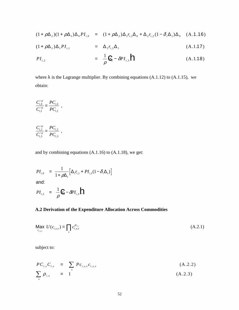
2.1 Expenditures Allocation Across Commodities

Domestic final consumption demand for each commodity takes the aggregate

consumption expenditure level previously chosen as given. In addition, we postulate that

the representative household of a country i maximizes a Cobb-Douglas utility function7:

7 An alternative way to state the problem is to consider the household as minimizing total expenditure (2.2.2), with anagregate level of consumption Ci,v being a Cobb-Douglas composite of the various commodities ci,s,v.

10

Maxc i s v i s v

si s v

i sU c c, ,

,) , , ( , , = ∏ ρ (2.2.1)

subject to:

PC C Pc ci v i v i s v i s vs

i ss

, , , , , ,

,

=

=

�

�

(2 .2.2)

(2 .2.3)ρ 1

where

ci s v, , : is consumption in country i of good s at period v,

Pi s v, , : is the price in country i of good s at period v,

ρi s, : is the share in country i of good s.

There are as many first order conditions as there are goods. The optimal consumption of a

given good s takes the following form8:

cPC C

Pci s v i si v i v

i s v, , ,

, ,

, ,

= ρ , (2.2.4)

where the aggregate price PCi,v: is given by:

PCPc

i vi s v

i ss

i s

,, ,

,

,

=FHG

IKJ∏ ρ

ρ

. (2.2.5)

Equation (2.2.4) implies that the share of aggregate consumption devoted to good s is the

product of the preference parameter for that good and its relative price.

8 See appendix for a complete derivation of this problem.

11

As for final consumption, the value of final investment demand for commodity s is also

generated by maximising aggregate investment, considered as a Cobb-Douglas composite

function of s investment goods, subject to the total investment expenditure level

determined in section 2.1. As a result, the final investment demand will take the same

form as (2.2.4), that is:

IPI IPii s v i s

i v i v

i s v, , ,

, ,

, ,

= ω , (2.2.6)

where ωi,s are share parameters in total investment and PIi,v the aggregate investment

price:

PIPi

i vi s v

i ss

i s

,, ,

,

,

=FHG

IKJ∏ ω

ω

. (2.2.7)

Equations (2.2.4) to (2.2.7) imply that the share of every good s in total consumption or

in total investment is constant.

Once the optimal level of each commodity s consumed and invested is determined, the

representative household of each country establishes the optimal composition of its

purchases in terms of specific purveyors.

2.3 Geographical Origins of Consumption and Investment goods

The representative household considers products of competitive industries from different

countries as imperfect substitutes [Armington (1969)], while it treats each good produced

by individual firms operating in non-competitive industries as specific [Dixit and Stiglitz

(1977)]. It is also assumed that firms do not discriminate between investors and

consumers, that is: the price charged by a firm f operating in country i to all customers is

12

the same, whether this customer uses its purchases for consumption or investment

purposes.

Formally, the preferences of the household in country i with respect to geographic or firm

origin are represented by a constant elasticity of substitution function (CES). The optimal

composition of its consumption basket in terms of geographic and firm origin is given by

the solution of the following optimisation problem:

Max c

c s

c sc i s v

j i s j i s vj

j i s j i s vfj

j i s v

c s i

c s i

c s i

c s i

cf s i

cf s i

cf s i

cf s i

f f

, , ,

, ,

, ,

, ,

, ,

, ,

, ,

, ,

, ,, ,

, , , , ,

, , , , , , ,

,

,

if is produced in a competitive sector

if is produced in a non-competitive sector,

=

LNMM

OQPP

LNMM

OQPP

R

S

||||

T

||||

− −

− −

�

��

δ

δ

σσ

σσ

σ

σ

σ

σ

1 1

1 1 (2.3.1)

subject to:

Pc c

P c s

P c si s v i s v

j i s v j i s v j i s vj

j i s v j f i s v j f i s vfj

, , , ,

, , , , , , , , ,

, , , , , , , , , , ,

( ) ,

( ) ,=

+

+

RS||T||�

��

1

1

τ

τ

if is competitive

if is non - competitive,(2.3.2)

where:

cj i s v, , , : consumption by country i of good s produced in country j at period v,

cj f i s v, , , , : consumption by country i of good s produced by non-competitive firm f of

country j at period v,

Pj i s v, , , : price in country i of good s produced in country j at period v,

13

Pj f i s v, , , , : price in country i of good s produced by non-competitive firm f of country j at

period v,

σ c s i, , : Armington elasticity of substitution for consumption in country i between good s

produced by competitive firms,

σ c s if , , : Dixit-Stiglitz elasticity of differentiation for consumption in country i between

good s produced by non-competitive firms,

δ c s i, , : consumption share parameters in country i for good s produced by competitive

firms,

δ c s if , , : consumption share parameters in country i for good s produced by non-

competitive firms,

τ j i s v, , , : tariff rate on good s purchased by country i from country j at period v.

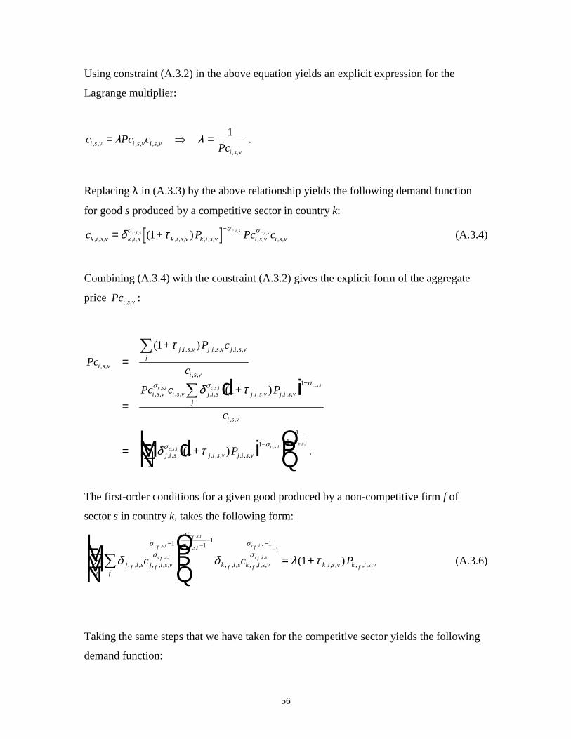
The first-order conditions for a given goods produced by a competitive sector s and

originating from a given country k takes the following form9:

c P Pc ck i s v k i s k i s v k i s v i s v i s vc i s c i s c i s

, , , , , , , , , , , , , , ,, , , , , ,( )= +

−δ τσ σ σ1 (2.3.3)

Combining (2.3.3) with the constraint (2.3.2) gives the explicit form of the aggregate

price Pci s v, , :

9 See the Appendix for a detailed derivation of the problem.

14

PcP c

c

Pc c P

c

P

i s v

j i s v j i s v j i s vj

i s v

i s v i s v j i s j i s v j i s vj

i s v

j i s j i s v j i s vj

c s i c s i c s i

c s i c s i c s i

, ,

, , , , , , , , ,

, ,

, , , , , , , , , , , ,

, ,

, , , , , , , ,

( )

( )

( ) .

, , , , , ,

, , , , , ,

=+

=+

= +LNM

OQP

�

�

�

−

− −

1

1

1

1

1

11

τ

δ τ

δ τ

σ σ σ

σ σ σ

d i

d i

(2.3.4)

This implies that the demand by an individual of country i for a good produced by a

competitive sector s in country k is function of the price of that good relative to price of

goods of type s in all other countries and of the quantity of good of type s the individual

wants to buy.

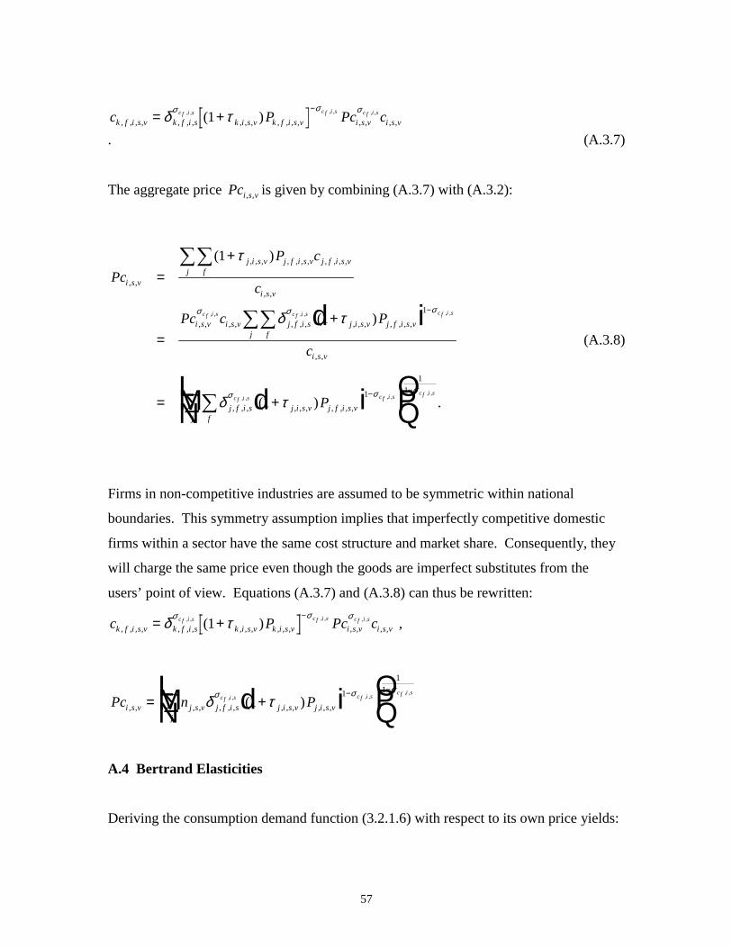
Similarly, the first-order conditions for a given good produced by a non-competitive firm

f of sector s in country k, takes the following form:

c P Pc ck f i s v k f i s k i s v k i s v i s v i s vc f i s c f i s c f i s

, , , , , , , , , , , , , , , , ,, , , , , ,( )= +

−δ τσ σ σ1 , (2.3.5)

Pc n Pi s v j s v j f i s j i s v j i s vj

c f i s c f i s c f i s

, , , , , , , , , , , , ,, , , , , ,

( )= +LNM

OQP

− −

� δ τσ σ σ

11

11d i , (2.3.6)

where nj,s,v is the number of firms in country j, sector s at time v.

The demand by an individual of country i for a good produced by firm f operating in a

non-competitive sector s of country k will therefore depends on the price of that good

relative to prices of goods of type s produced by all other firms around the world and on

the quantity of good s the individual wants to buy overall.

15

From equations (2.3.5) and (2.3.6), we can see that an increasing the number or varieties

of goods displays increasing returns (Ethier, 1982). An increase in the number of firms

reduces the relative price (vsi

vsij

PcP

,,

,,, ) of all existing goods and thus raises their demand.

As in the case of the consumption basket, the optimal investment composition in terms of

its geographic or firm origins is obtained from a maximisation of a CES composite of

investment goods s from all possible origins, subject to an investment expenditure level

as determined in section 2.2. As a result, the final investment demands take an identical

form to (2.3.3) and (2.3.5). For good s originating from competitive firms, we have:

i P Pi Ij i s v j i s j i s v j i s v i s v i s vI i s I i s I i s

, , , , , , , , , , , , , , ,, , , , , ,( )= +

−β τσ σ σ1 ; (2.3.7)

and for s originating from non-competitive firms, we have:

i P Pi Ij f i s v j f i s j i s v j i s v i s v i s vI f i s I f i s I f i s

, , , , , , , , , , , , , , , , ,, , , , , ,( )= +

−β τσ σ σ1 , (2.3.8)

where the β are share parameters. The aggregate investment prices also have forms that

are similar to the aggregate consumption prices. For good s produced by competitive

firms, we have:

Pi Pi s v j i s j i s v j i s vj

I s i I s i I s i

, , , , , , , , , ,, , , , , ,

( )= +LNM

OQP

− −

�β τσ σ σ

11

11d i , (2.3.9)

and for goods produced by non-competitive firms, we have:

Pi n Pi s v j s v j i s j i s v j i s vj

f

I f i s I f s i I f i s

, , , , , , , , , , , , ,, , , , , ,

( )= +LNM

OQP

− −

� β τσ σ σ

11

11d i . (2.3.10)

The combined Cobb-Douglas/CES functional forms on which these demand functions are

based are commonly used in the literature. They are convenient for both computational

16

and calibration procedures and require data on a smaller number of parameters than other

more flexible functional forms.

3. The Firms

In each country, there are competitive and non-competitive sectors. In both sectors, the

technology of production requires that firms employ capital, labour and intermediate

inputs to produce output. Material inputs are introduced in the production function in a

way similar to the way consumption goods are treated in the preferences of households:

with an Armington specification for goods produced by competitive sectors and with an

Ethier (1982) specification (i.e., with product differentiation at the firm level) in the

imperfectly competitive sectors. Firms are assumed to be profit maximising and each

firm produces one product, and in only one sector.

Labour and capital are assumed to be homogeneous and mobile between sectors within

national boundaries. There is no international labour or capital mobility. Therefore, the

wage and rental rate is the same across sectors within a given country, but may differ

across countries. Labour is supplied inelastically by domestic consumers.

3.1 Competitive industries

In competitive industries, the representative firm operates with constant returns to scale

technologies and behaves as a price taker on products as well as on factor markets. This

firm’s objective is to maximise its profits:

Max Qi,s,v

P Q v Qi s v i s v i s v i s v, , , , , , , ,− ,

where Qi,s,v and vi,s,v represent for country i, sector s, and period v, the production level

and the marginal cost respectively. The first-order condition to this problem is the usual

equality between price and marginal cost:

17

P vi s v i s v, , , ,= . (3.1.1)

Taking price as given, the firm’s unit cost and hence factors and materials demands are

determined by the following total cost minimization problem:

Min v Q w L r K Px Xi s v i s vL K X

i v i s v i v i s v i sd s v i sd s vsdi s v i s v i sd s v

, , , ,, ,

, , , , , , , , , , , ,, , , , , , ,

= + +� , (3.1.2)

subject to a (Cobb-Douglas) technology:

Q L K Xi s v i s v i s v i sd s vsd

Li s Ki s xi sd s, , , , , , , , ,

, , , ,= ∏α α α , (3.1.3)

where:

wi v, : wage rate in country i at period v,

Li s v, , : quantity of labour in sector s at period v,

ri v, : rental rate of capital in country i at period v,

Ki s v, , : stock of capital in sector s at period v,

Pxi sd s v, , , : average price paid by sector s of country i for goods sd at period v,

Xi sd s v, , , : average price paid by sector s of country i for goods sd at period v,

α s : share parameters.

Assuming constant returns to scale, the share parameters sum to one:

α α αL K Xsd

i s i s i sd s, , , ,+ + =� 1 . (3.1.4)

The first order conditions to this problem yield the demand conditions. First, for labour:

18

Lv Qwi s v

L i s v i s v

i v

i s

, ,, , , ,

,

,=α

; (3.1.5)

second, for capital:

Kv Qri s v

K i s v i s v

i v

i s

, ,, , , ,

,

,=α

; (3.1.6)

and third, for inputs originating from sector sd:

Xv Q

Pxi sd s vX i s v i s v

i sd s v

i sd s

, , ,, , , ,

, , ,

, ,=α

. (3.1.7)

Equations (3.1.5) to (3.1.7) imply that the proportions of labour cost, capital cost, and

intermediate good cost in total cost are constant. Substituting these demand functions

into the production function (3.1.3) gives:

Qv Qw

v Qr

v QPx

v Qw r

i s vL i s v i s v

i v

K i s v i s v

i v

X i s v i s v

i sd s vsd

i s v i s vL

i v

K

i v

i s

Li s

i s

Ki s

sd s i

Xi sd s

Lis Ki s Xi sd ssd

i s

Li s

i s

, ,, , , ,

,

, , , ,

,

, , , ,

, , ,

, , , ,, ,

,

,

,

,

, ,

, ,

, , , ,

,

,

=FHG

IKJ

FHG

IKJ

FHG

IKJ

= � FHG

IKJ

FHG

IK

∏+ +

α α α

α α

α α α

α α αα

c h J FHG

IKJ

=FHG

IKJFHG

IKJ

∏

∏ ∏− − −

α α

α α α α α α

α

α α α

Ki s

i sd s

Xi sd s

i s

Li si s

Ki si sd s

Xi sd s Li s Ki s Xi sd s

X

i sd s vsd

i s v i s v L K Xsd

i v i v i sd s vsd

Px

v Q w r Px

,

, ,

, ,

,,

,,

, ,, , , , , ,

, , ,

, , , , , , , , , .

The above yields the unit cost function:

19

vA

w r Px

A

i s vi s

i v i v i sd s vsd

i s L K Xsd

Li s Ki s Xi sd s

i s

Li si s

Ki si sd s

Xi sd s

, ,,

, , , , ,

,

, , , ,

,,

,,

, ,, ,

,=FHG

IKJ

=FHG

IKJ

∏

∏

1 α α α

α α αα α α

where

is a constant.

(3.1.8)

Since materials and factors prices are given to the representative firm in competitive

sector s of country i, equations (3.1.5) to (3.1.7) determine its factor demands, while

equations (3.1.1) and (3.1.8) determines its optimal supply. Given the constant returns to

scale technology, the level of production and the inputs demanded by industry s are

determined by the demand side of the market.

As for households, the representative firm considers intermediate inputs from competitive

industries of different countries to be imperfect substitutes and inputs from non-

competitive industries to be specific to the different firms. Therefore, firm s in country i

needs to choose from which regions and firms it purchases its intermediate inputs. The

firm's preference with respect to geographical and firm origin of a commodity sd is

assumed to be a CES aggregation function of inputs from all possible sources. The

solution to the following problem determines the share from each origin:

Max

if is produced by competitive firms,

if is produced by non - competitive firms,

X

X sd

X sd

i sd s v

j i sd s j i sd s vj

j f i sd s j f i sd s vfj

x s i

x s i

x s i

x s i

x f s i

x f s i

x f s i

x f s i

, , ,

, , , , , , ,

, , , , , , , , ,

, ,

, ,

, ,

, ,

, ,

, ,

, ,

, ,

,

,

=

LNMM

OQPP

LNMM

OQPP

R

S||||

T||||

− −

− −

�

��

η

η

σσ

σσ

σ

σ

σ

σ

1 1

1 1

subject to:

20

Px X

P X sd

P X sdi sd s v i sd s v

j i sd v j i sd v j i sd s vj

j i sd v j f i sd v j f i sd s vfj

, , , , , ,

, , , , , , , , , ,

, , , , , , , , , , , ,

( ) ,

( ) ,=

+

+

RS||T||�

��

1

1

τ

τ

if originates from competitive firms,

if originates from non - competitive firms,

where:

X j i sd s v, , , , : amount of intermediate inputs purchased by sector s of country i from

sector sd in country j at period v,

X j f i sd s v, , , , , : amount of intermediate inputs purchased by sector s of country i from firm

f of sector sd in country j at period v,

Pj i sd v, , , : price of goods sd sold by country j to country i at period v,

Pj f i sd v, , , , : price of goods sd sold by firm f of country j to country i at period v,

α s : share parameters,

σ x s i, , : Armington elasticity of substitution of sector s in country i at period v, for

intermediate inputs produced by competitive firms,

σ x s if , , : Dixit-Stiglitz elasticity of substitution of sector s in country i at period v,

for intermediate inputs produced by non-competitive firms f.

Taking the same steps as for the consumption problem (section 2.3), the demand function

for a given intermediate input sd from country j is given by the following equation if sd

originates from competitive firms:

X P Px Px Xj i sd s v j i sd v j i sd v i sd s v j i sd s i sd v i sd s vx s i x s i

, , , , , , , , , , , , , , , , , , , , ,( ) , , , ,= +− −1 1τ η

σ σ σ , (3.1.9)

where:

Px Pi sd s v j i sd s j i sd v j i sd vj

x i s x i s x i s

, , , , , , , , , , , ,, , , , , ,

( )= +LNM

OQP

− −

� η τσ σ σ

11

11d i .

21

As for consumption goods, the demand by firm f in country i for an intermediate good

produced by a competitive sector s in country k is function of the price of that

intermediate good relative to the price of intermediate goods of type s in all other

countries and the quantity of intermediate good of type s this firm wants to buy overall.

If sd originates from non-competitive firms, the demand function is given by:

X P Px Px Xj i sd s v j i sd v j i sd v i sd s v j i sd s i sd v i sd s vf

x f i s x f i s

f

x f i s

, , , , , , , , , , , , , , , , , , , , , ,( ) , , , , , ,= +− −1 1τ η

σ σ σ , (3.1.10)

where

Px n Pi sd s v j sd v j f i sd s j i sd v j i sd vj

x f i s x f i s x f i s

, , , , , , , , , , , , , , ,, , , , , ,

( )= +LNM

OQP

− −

� η τσ σ σ

11

11d i .

As for consumption goods, the demand by firm f in country i for an intermediate good

produced by sector s in country k is therefore function of the price of that intermediate

good relative to the price of intermediate goods of type s in all other firms around the

world and the quantity of intermediate good of type s this firm wants to buy overall.

3.2 Non-Competitive sectors

The number of firms in non-competitive industries is endogenous. As noted earlier, firms

in the same sector within national boundaries are symmetric, and therefore, have the

same increasing returns to scale technology. Increasing returns are obtained by assuming

that the set up of a firm requires a fixed bundle of capital and labour. In other words,

firms face fixed primary factor costs. These introduce a wedge between total unit costs

of the non-competitive firm f from sector s in country i (VTi,f,s,v) and its marginal costs

(vi,f,s,v):

22

VT vw L r K

Qi s v i s vi v i s i v i s

i s vf f

f f

f, , , , , ,

, , , , , ,

, , ,

= ++

,

where Li sf, , and Ki sf, , denote the firm’s fixed labour and capital respectively. With such

a set-up, total unit costs decline asymptotically to unit variable costs. The ratio of

marginal to average cost is conventionally used to measure the extent of unexploited

scale economies.

Regions or countries are considered segmented markets for many reasons. First, in

industries characterized by product differentiation, price discrimination between different

national markets is common, as there is no effective means of arbitrage. Second, the

presence of various forms of non-tariff barriers prevents cross-border price arbitraging.

Much of the empirical evidence on market segmentation has been drawn from the

experience of the United States in the 1980s, when the dollar underwent a massive

appreciation and subsequent depreciation. During these swings in the value of the dollar,

foreign producers charged prices in U.S. markets that were different in comparison with

those charged in other markets. Firms were choosing to “price to market”10. This has

called into question theories that rely upon the concept of spatial arbitrage in goods.

Krugman (1989) summarizes this by noting that: “Not only does the Law of One Price

fail to hold at the level of aggregate national price indices, it doesn’t even hold at the

level of individual goods.” The absence of spatial arbitrage allows prices to diverge

across markets. This view, which is adopted in the present paper, favours market

segmentation rather than integration, and thereby acknowledges the presence of

economic barriers and structural rigidities restricting convergence in inter-market prices.

As a consequence, the non-competitive firm facing demand segmentation takes

advantage of the monopoly power it has on each country’s market. For this purpose, the

firm is endowed with the knowledge of the preferences and technologies of its clients.

10 See, for example, Krugman (1987,1989), Mann (1987), Dornbush (1987), Giovannini (1988), Marston(1990).

23

Moreover, product differentiation and monopoly power raise the issue of strategic

interaction between firms. Several specifications for modelling this is available, as there

are different ways for firms to behave in an oligopolistic environment. In this model we

consider two possible strategic behaviours: non co-operative Bertrand behaviour, and non

co-operative Cournot behaviour.

3.2.1 The Bertrand Case

In the Bertrand case, the firm determines the price level that maximises its profit given

the preferences and technologies of its clients, and assuming that its competitors keep

their prices fixed at their current levels. In order to simplify the computation procedure

we also assume that in each country, each consumer’s current-price expenditures on the

whole industry is unaffected by the strategic decisions of the firm considered. As

advocated in the theoretical literature (Hart, 1985) and highlighted by Roberts and

Sonnenschein (1977), and Dierker and Grodal (1986), this assumption permits the

neutralisation of the non-existence of equilibrium problem. However, another

implication is that firms make decisions with systematic errors. The relevant question is

whether these systematic errors significantly affect the model’s predictions. This is an

important empirical issue that has not yet been addressed.

Formally, the maximisation problem for a firm f of country i is:

Max P q v q w L r KP i j s v i f j s v i f j s v i f s v i f j s v

ji v i f s i v i f s

i f j s vf

, , , ,, , , , , , , , , , , , , , , , , , , , , , , , ,

j

π = − − −� � , (3.2.1.1)

q c i xi f j s v i f j s v i f j s v i f j s sd vsd

, , , , , , , , , , , , , , , , ,= + +� , (3.2.1.2)

where qi,f,j,s is what firm f in country i perceives as the demand for goods s from

consumers, investors and other firms of country j.

24

For each good s sold by firm f of country i to country j, the first-order conditions to this

problem are:

Pq P

vi f j s vi f j s v i f j s v

i f s v, , , ,, , , , , , , ,

, , ,( , )1 1 +FHG

IKJ=

ε , (3.2.1.3)

where:

ετ

( , )( ), , , , , , , ,, , , ,

, , , , , ,

q PLog q

Log Pi j s v i j s vi j s v

i j s v i j s vf f

f=∂

∂ +

1d i (3.2.1.4)

is the definition of the Bertrand direct price elasticity of demand of goods s from firm f.

The smaller is the elasticity, the higher is the price the firm will charge. This elasticity is

given by simple differentiation of the demand function with respect to price Pi,f,j,s. When

firm f increases its price, the quantity it sells diminishes and the industry average price

increases. This pushes up the quantity sold by the other firms. Since other firms are

assumed to keep their prices unchanged and the demand for the firm’s good is function

only of the relative price [equations 2.3.5, 2.3.8, and 3.1.10], this increase in quantity sold

doesn't affect the firm’s strategy.

The demand addressed to the firm being the sum of the demand for consumption,

investment and intermediate goods, the total derivative of (3.2.1.4) is equal to the

weighted sum of the derivatives:

25

ε ε

ε

ε

( , ) ( , )

( , )

( ,

, , , , , , , , , , , , , , , ,, , , , , , , ,

, , , , , , , ,

, , , , , , , ,, , , , , , , ,

, , , , , , , ,

, , , , , , , ,

q P c PP cP q

i PP iP q

x P

i f j s v i f j s v i f j s v i f j s vi f j s v i f j s v

i f j s v i f j s v

i f j s v i f j s vi f j s v i f j s v

i f j s v i f j s v

i f j s sd v i f j sh h

=

+

+ ,, , , , , , , , ,

, , , , , , , ,

) .vsd

i f j s v i f j s sd v

i f j s v i f j s v

P xP q

h�

(3.2.1.5)

Since we assume that all firms in a noncompetitive sector of a given country are

symmetric, we omit the subscript f on the price variable in the remainder of this section.

For the consumption goods, the demand function addressed to country firm f by

consumers of country j for goods s at period v is given by combining (2.3.5) and (2.3.6):

c P Pc Pc c

P n P

i f j s v i f j s i j s v i j s v j s v j s v j s v

i f j s i j s v i j s v i s v i f j s i j s v i j s vi

cf j s cf j s cf j s

cf j s cf j s cf j s cf j s

, , , , , , , , , , , , , , , , , , ,

, , , , , , , , , , , , , , , , , , , ,

, , , , , ,

, , , , , , , ,

( )

( ) ( )

= +

= + +LNM

O

− −

− −�

δ τ

δ τ δ τ

σ σ σ

σ σ σ σ

1

1 1

1

1

QP= + +L

NMOQP

−

−

− −−

�

σ

σ

σ σ σ σδ τ δ τ

cf j s

cf j s

cf j s cf j s cf j s cf j s

Pc c

P n P Pc c

j s v j s v

i f j s i j s v i j s v i s v i f j s i j s v i j s vi

j s v j s v

, ,

, ,

, , , , , , , ,

, , , ,

, , , , , , , , , , , , , , , , , , , , , , , ,( ) ( )

1

1

11

1 1

(3.2.1.6)

Combining equation (2.2.2) with the above assumption that firms consider current-price

expenditure of their clients on the whole industry unaffected by their own action, means

that the nominal expenditure share for a given sector s:

ρ j sj s v j s v

j v j v

Pc cPC C,

, , , ,

, ,

=

is constant. This implies that the firm cares about the effect of its price on the quantity

sold by its competitors in its sector but not on the quantity sold by its competitors in other

sectors.

26

Deriving the consumption demand function (3.2.1.6) with respect to its own price11 yields

the Bertrand price elasticity:

ε σ στ

( , ) ( )( )

, , , , , , , , , , ,, , , , , , , , , ,

, , , ,

c PP c

Pc ci j s v i j s v c j s c j si j s v i j s v i j s v

j s v j s vf

f

f f= − − −

+1

1d i . (3.2.1.7)

If we derive the consumption demand function (3.2.1.6) with respect to the price of a

country k competitor, we obtain the Bertrand cross-price elasticity:

ε στ

( , ) ( )( )

, , , , , , , , ,, , , , , , , , ,

, , , ,

c PP c

Pc ci j s v k j s v c j sk j s v k j s v k j s v

j s v j s vf f

= − −+

11d i

. (3.2.1.8)

Similar Bertrand elasticities can be defined and derived for both investment demand:

ε σ στ

( , ) ( )( )

, , , , , , , , , , ,, , , , , , , , ,

, , , ,

i PP i

Pi ii j s v i j s v i j s i j si j s v i j s v i j s v

j s v j s vf f f

f= − − −+

11d i

, (3.2.1.9)

and for intermediate goods demand:

ε σ στ

( , ) ( )( )

, , , , , , , , , , , ,, , , , , , , , , , ,

, , , , , ,

X PP X

Px Xi j s sd v i j s v x j s x j si j s v i j s v i j s sd v

j s sd v j s sd vf

f

f f= − − −

+1

1d i . (3.2.1.10)

The perceived elasticity used by firm f is given by replacing equations (3.2.1.7), (3.2.1.9)

and (3.2.1.10) in equation (3.2.1.5). The quantity sold by the firm to any country j is

determined by this elasticity and equations (3.2.1.3) and (3.1.8). The sum of these sales

yields the level of production of a non-competitive firm f:

11 See Appendix for Details

27

Q qi f s v i f j s vj

, , , , , , ,=� . (3.2.1.11)

Since firms are assumed symmetric within national boundaries, the total production of a

non-competitive sector s is:

Q n Qi s v i s v i f s v, , , , , , ,= . (3.2.1.12)

Combining this level of production with equations (3.1.7) to (3.1.9) yields the quantity of

labour, capital, and intermediate inputs used by non-competitive sector s.

As for the household and the representative competitive firm, non-competitive firms

consider intermediate inputs from competitive industries of different countries, and inputs

from non-competitive industries of different firms, to be imperfect substitutes. A non-

competitive firm thus has to choose from which firms and regions it purchases its

intermediate inputs. The intermediate input demand functions of a non-competitive firm

are determined, as for competitive firms, by equations (3.1.9) and (3.1.10).

3.2.2 The Cournot Case

In the Bertrand case, imperfect competitors treat price levels as their strategic variables.

Firms choose their prices and let the market determine the quantity sold. Another

approach is to think of firms as setting their quantities while the market determines

prices. This kind of behaviour is known as Cournot competition. As in the Bertrand

case, the non-competitive firm performs a profit maximisation calculation assuming that

other firms’ strategic variables are unaffected by its own strategic action. Therefore, in

the Cournot framework, the maximising firm assumes that the quantity sold by other

firms is not affected by its own strategy. The formal maximisation problem for firm f of

country i is:

28

Max P q v q w L r Kq i j s v i f j s v i f j s v i s v i f j s v

ji v i f s i v i f s

i f j s vff

, , , ,, , , , , , , , , , , , , , , , , , , , , , , ,

j

π = − − −� � (3.2.2.1)

subject to:

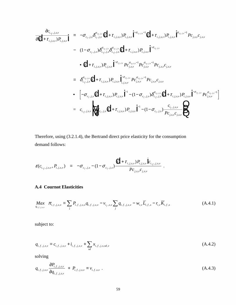
q c i xi f j s v i f j s v i f j s v i f j s sd vsd

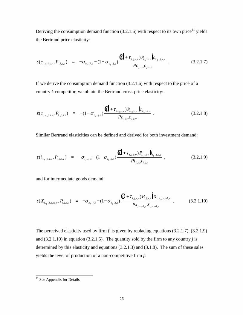
, , , , , , , , , , , , , , , , ,= + +� (3.2.2.2)

Solving this problem yields the following first-order condition:

where:

ε( , ), , , , , , , ,, , , ,

, , , ,

P qLog PLog qi f j s v i f j s v

i f j s v

i f j s v

=∂∂

(3.2.2.3)

is the Cournot direct-quantity elasticity of demand for goods s from firm f. In contrast to

the Bertrand case, the Cournot price elasticity cannot be obtained by simply

differentiating the demand function. In the Cournot case, an increase of the output firm f

raises its profits since it is selling a larger quantity of goods at the current price. As the

competitors are assumed to keep their quantity sold unchanged, the increase in industry

output pushes the price down. This decline in price reduces the firm’s profits over all the

other units it is selling. The magnitude of this price reduction depends on the reaction of

other firms to the output increase. The optimizing firm has thus to forecast other firms’

reaction functions in order to make rational decisions about its own output choice. The

Cournot equilibrium is reached when each firm’s forecast about other firms behaviour is

consistent.

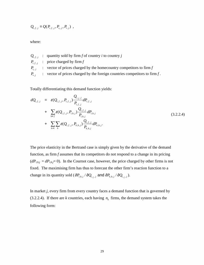
The demand function of country j for goods produced by firm f of country i can be

expressed as:

P P q vi f j s v i f j s v i f j s v i f s v, , , , , , , , , , , , , , ,( , )1 + =εd i

29

Q Q P P Pi f j i f j i j j, , , , , ,( , , )=• • ,

where:

Q f i jP fP fP f

i f j

i f j

i j

j

, ,

, ,

,

, .

: quantity sold by firm of country to country : price charged by firm : vector of prices charged by the homecountry competitors to firm : vector of prices charged by the foreign countries competitors to firm

•

•

Totally differentiating this demand function yields:

dQ Q PQ

PdP

Q PQP

dP

Q PQP

dP

i f j i f j i f ji j

i f ji f j

i f j i h jh f

i f j

i h ji h j

i f j k h jhk i

i f j

k h jk h j

f, , , , , ,

, ,

, ,, ,

, , , ,, ,

, ,, ,

, , , ,, ,

, ,, ,

( , )

( , )

( , ) .

=

+

+

≠

≠

�

��

ε

ε

ε

(3.2.2.4)

The price elasticity in the Bertrand case is simply given by the derivative of the demand

function, as firm f assumes that its competitors do not respond to a change in its pricing

(dPi,h,j = dPi,k,j= 0). In the Cournot case, however, the price charged by other firms is not

fixed. The maximising firm has thus to forecast the other firm’s reaction function to a

change in its quantity sold ( ∂ ∂ ∂ ∂P Q P Qi h j i j k h j i jf f, , , , , , , ,/ / and ).

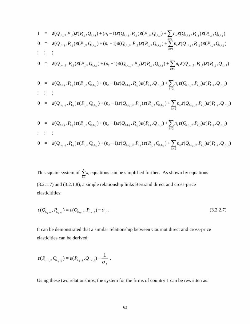
In market j, every firm from every country faces a demand function that is governed by

(3.2.2.4). If there are k countries, each having nk firms, the demand system takes the

following form:

30

dQQ

Q PdPP

dQQ

Q PdPP

dQQ

Q PdPP

j

jj k j

h

n

k

K k j

k j

j

jj k j

h

n

k

K k j

k j

j

jj k j

h

n

k

K k j

k j

hh

h

hh

h

n

nn h

h

h

k

k

k

1,1

1,11,1

1,2

1,21,2

1

11

11

11

11

1

1

1

,

,, , ,

, ,

, ,

,

,, , ,

, ,

, ,

, ,

, ,, , , ,

, ,

, ,

( , )

( , )

( , )

= ��

= ��

= ��

==

==

==

ε

ε

ε

� � �

dQQ

Q PdPP

dQQ

Q PdPP

j

jj k j

h

n

k

K k j

k j

j

jj k j

h

n

k

K k j

k j

hh

h

n

nn h

h

h

k

k

2 1

2 12 1

2

22

11

11

1

2

2

, ,

, ,, , , ,

, ,

, ,

, ,

, ,, , , ,

, ,

, ,

( , )

( , )

= ��

= ��

==

==

ε

ε

� � �

dQQ

Q PdPP

dQQ

Q PdPP

K

KK h

h

h

K n

K nK n h

h

h

j

jj k j

h

n

k

K k j

k j

j

jj k j

h

n

k

K k j

k j

k

kk

k

k

, ,

, ,, , , ,

, ,

, ,

, ,

, ,, , , ,

, ,

, ,

( , )

( , ) .

1

11

11

11

= ��

= ��

==

==

ε

ε

� � �

The Cournot behaviour implies that each firm makes a decision about its output by

solving this system and assuming that other firms’ output remain unaffected by its own

strategic action. Since all firms of a particular country i are symmetric, the system for the

firms of country i is the following12:

12 See Appendix for details

31

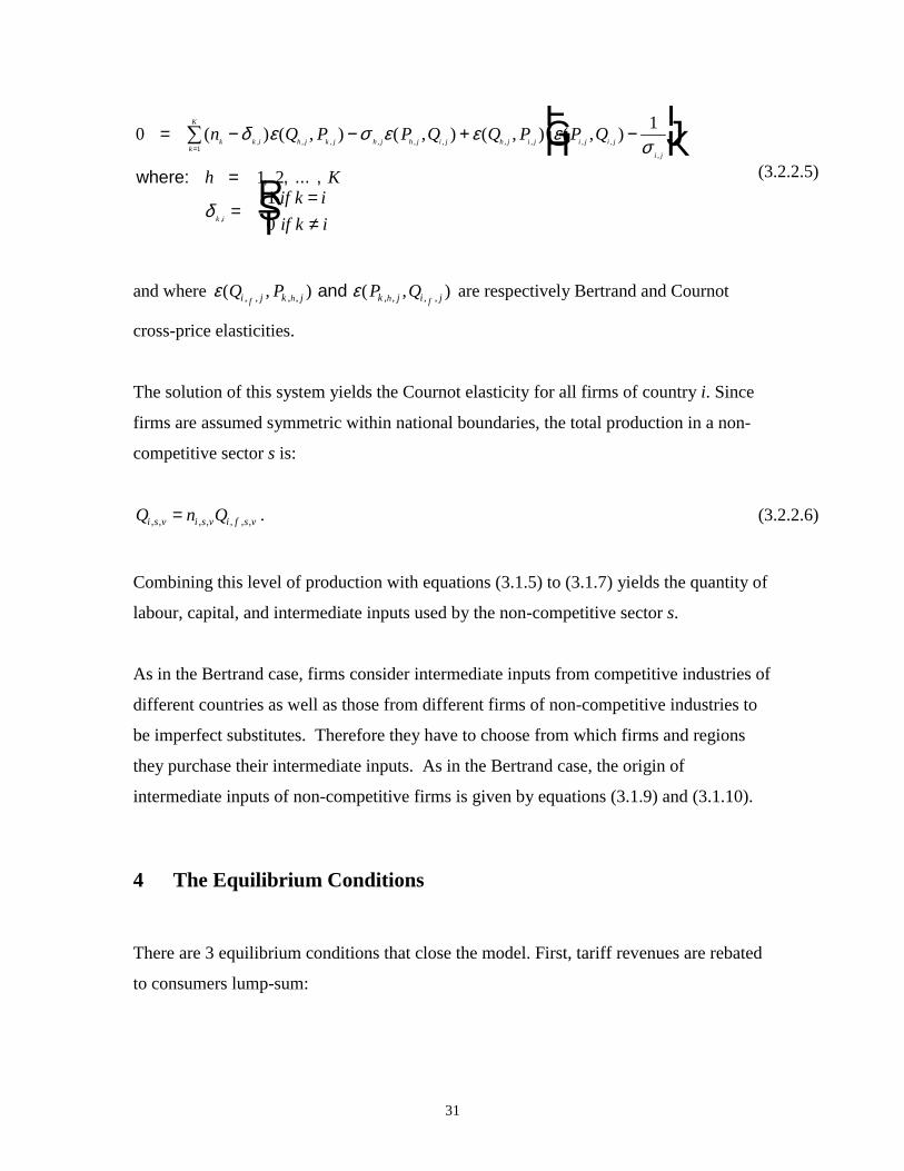
0 1

1 210

1=

where: , , ... , =

( ) ( , ) ( , ) ( , ) ( , ), , , , , , , , , ,

,

,

n Q P P Q Q P P Q

h Kif k iif k i

k k i h j k j h j h j i j h j i j i j i j

i jk

K

k i

− − + −FHG

IKJ

=

=≠

RST

=� δ ε σ ε ε ε

σ

δ

(3.2.2.5)

and where ε ε( , ) ( , ), , , , , , , ,Q P P Qi j k j k j i jf h h f and are respectively Bertrand and Cournot

cross-price elasticities.

The solution of this system yields the Cournot elasticity for all firms of country i. Since

firms are assumed symmetric within national boundaries, the total production in a non-

competitive sector s is:

Q n Qi s v i s v i f s v, , , , , , ,= . (3.2.2.6)

Combining this level of production with equations (3.1.5) to (3.1.7) yields the quantity of

labour, capital, and intermediate inputs used by the non-competitive sector s.

As in the Bertrand case, firms consider intermediate inputs from competitive industries of

different countries as well as those from different firms of non-competitive industries to

be imperfect substitutes. Therefore they have to choose from which firms and regions

they purchase their intermediate inputs. As in the Bertrand case, the origin of

intermediate inputs of non-competitive firms is given by equations (3.1.9) and (3.1.10).

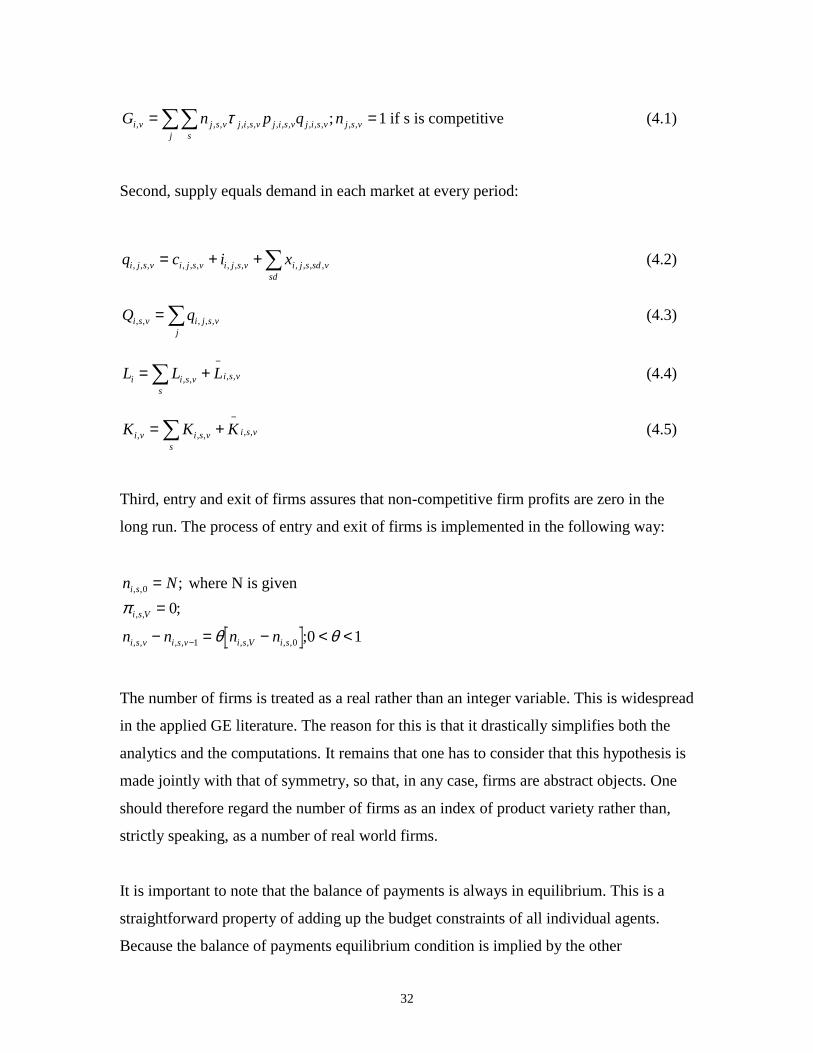
4 The Equilibrium Conditions

There are 3 equilibrium conditions that close the model. First, tariff revenues are rebated

to consumers lump-sum:

32

G n p q ni v j s vs

j i s v j i s v j i s v j s vj

, , , , , , , , , , , , , ,;= =�� τ 1 if s is competitive (4.1)

Second, supply equals demand in each market at every period:

q c i xi j s v i j s v i j s v i j s sd vsd

, , , , , , , , , , , , ,= + +� (4.2)

Q qi s v i j s vj

, , , , ,=� (4.3)

L L Li i s v i s vs

= +−

� , , , , (4.4)

K K Ki v i s v i s vs

, , , , ,= +−

� (4.5)

Third, entry and exit of firms assures that non-competitive firm profits are zero in the

long run. The process of entry and exit of firms is implemented in the following way:

n N

n n n n

i s

i s V

i s v i s v i s V i s

, ,

, ,

, , , , , , , ,

;;

;

0

1 0

0

0 1

==

− = − < <−

where N is givenπ

θ θ

The number of firms is treated as a real rather than an integer variable. This is widespread

in the applied GE literature. The reason for this is that it drastically simplifies both the

analytics and the computations. It remains that one has to consider that this hypothesis is

made jointly with that of symmetry, so that, in any case, firms are abstract objects. One

should therefore regard the number of firms as an index of product variety rather than,

strictly speaking, as a number of real world firms.

It is important to note that the balance of payments is always in equilibrium. This is a

straightforward property of adding up the budget constraints of all individual agents.

Because the balance of payments equilibrium condition is implied by the other

33

equilibrium conditions, it is not necessary to explicitly impose a balance of payments

equilibrium condition.

5. Data Requirements and Calibration Strategy

An appropriate calibration procedure for the model must be based on a multi-country

multi-sector database. Such a database requires the collection of data from national and

international publications. In these publications, we usually find nominal bilateral trade

flows, national accounts data (consumption and investment demands by sector, labour

and capital earnings), and input-output tables. Moreover, consistency among the sources

needs to be ensured13.

Constructing a consistent multi-country multi-sector database is a difficult and tedious

task. It may be preferable to use an existing database, as for instance GTAP14. The

GTAP database combines detailed consistent data across 30 regions and 37 sectors. In

the literature, this database has been used extensively for a wide variety of questions

ranging from trade to environment. Once the database is ready, the calibration procedure

follows three steps.

5.1 Balancing the Social Accounting Matrix

The first step is to balance the social accounting matrix for every country, i.e. to ensure a

consistent benchmark data set. The social accounting matrices are said to be balanced

when four major sets of equilibrium conditions are satisfied: (i) supply equals demand for

all commodities; (ii) all industries make no profits; (iii) all domestic agents’ budget

constraints are satisfied; and finally (iv) bilateral trades are consistent, i.e. domestic

external balances sum to zero.

13 For example, the sum of balance of payments across countries must be nil.

34

5.2. Calibrating the supply side of the model

The calibration of the supply side determines initial markups and elasticities for non-

competitive firms, as well as the different share parameters in the unit cost function for

all firms.

5.2.1 Determining initial markups and elasticities

The Bertrand elasticities depend on the Dixit-Stiglitz differentiation elasticities, on the

number of firms, and on the market share the exporting country has in the client market.

Reasonable estimates for the Dixit-Stiglitz differentiation elasticities can be inferred from

the literature. The number of firms in non-competitive sectors is inferred from

Herfindahl or other industry concentration indices. The market shares exporting country

i has in the client market j is expressed as:

( );

( );

( ), , , , , , ,

, ,

, , , , , , ,

, ,

, , , , , , , , ,

, , , , ,

1 1 1+ + +τ τ τi j s i j s i f j s

j s j s

i j s i j s i f j s

j s j s

i j s i j s i f j h s sd

j s sd j h s sd

P cPc C

P iPi I

P XPx X

.

Since firms are symmetric, we have:

( ) ( )

( ) ( )

( ) (

, , , , , ,

, ,

, , , , , ,

, , ,

, , , , , ,

, ,

, , , , , ,

, , ,

, , , , , , ,

, , , ,

, ,

1 1

1 1

1 1

+=

+

+=

+

+=

+

τ τ

τ τ

τ τ

i j s i j s i f j s

j s j s

i j s i j s i j s

i s j s j s

i j s i j s i f j s

j s j s

i j s i j s i j s

i s j s j s

i j s i j s i f jh s sd

j s sd jh s sd

i j s

P cPc C

P cn Pc C

P iPi I

P in Pi I

P xPx X

) , , , , ,

, , , , ,

P xn Px X

i j s i j s sd

i s j s sd j s sd

Data on country j final consumption, investment and intermediate uses of goods s by

geographical origin i (ci,j,s , ii,j,s , xi,j,s,sd) are usually not available. However, the share of

imported to total consumption of goods s [θcj,s] and the decomposition of total imports of 14 Global Trade Analysis Project Data Base, version 3, Purdue University.

35

goods s [ej,s] by origin [ei,j,s] are available. We can then use the proportion of each origin

in total imports of goods s [ei,j,s / ej,s] to total imports of consumption goods s

[θcj,sPcj,sCj,s], to approximate the imported consumption by geographical origin:

( ), , , , , , , , , , , ,1+ =τ θi j s i j s i j s i j s j s j s j s j sP c e e Pc C .

The consumption demand satisfied by domestic firms is simply:

P c c Pc Cj j s j j s j s j s j s, , , , , , ,( )= −1 θ .

The same procedure is used for investment goods imported by geographical origin and

domestic investments:

( )

( ), , , , , , , , , , , ,

, , , , , , ,

11

+ == −

τ θθ

i j s i j s i j s i j s j s j s j s j s

j j s j j s j s j s j s

P i e e i Pi IP i i Pi I

whereas for intermediate goods, we have:

( )( )

, , , , , , , , , , , , , , , ,

, , , , , , , , , , ,

11

+ == −

τ θθ

i j s i j s i j s sd i j s j s j s sd j s sd j s sd

j j s j j s sd j s sd j s sd j s sd

P x e e x Px XP x x Px X

Once imports by geographical origin are calibrated for each country j, the market shares

of each exporting country i can be established and estimates for Bertrand elasticities can

be calculated. Using these elasticity estimates in equation system (3.2.2.5) enables us to

determine Cournot elasticities.

The next step is to calibrate the markups at the benchmark equilibrium. After some

simple manipulations, we can obtain the price to variable unit cost ratio:

36

Pv

q Pq P

i j s

i s

i f j s i j s

i f j s i j s

, ,

,

, , , , ,

, , , , ,

( , )( , )

;=+

εε 1

in the Bertrand case , (5.2.1.1)

Pv P q

i j s

i s i j s i f j s

, ,

, , , , , ,( , );=

+1

1 ε in the Cournot case , (5.2.1.2)

where:

P qn

P c i x

en

i j s i f j s

i s

i j s i j s i j s i j s sdsd

i j s

i s

, , , , ,

.

, , , , , , , , ,

, ,

,

= + +FH IK=

�1

Define Pi s, as the average selling price of the firm operating in non-competitive sector s

of country i; then by definition Pi s, satisfies:

P q ei s i j s i j sjj

, , , , ,= �� .

This equation can be rewritten as:

Pv

ePv

ei s

i s

i j s

i j s

i s

i j sjj

,

,

, ,

, ,

,

, ,LNM

OQP

= �� . (5.2.1.3)

By normalising Pi s, to unity, equations (5.2.1.3) and (5.2.1.1) jointly determine the

variable unit costs vi,s, and the segmented-market price system consistent with the data set

and with preferences under the Bertrand competitive game. Alternatively, we can

determine the system under the Cournot game.

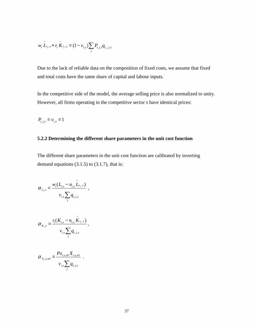
The assumption of zero pure profits determines the fixed costs as follows:

37

w L r K v P qi i s i i s i s i j s i j sj

f f f

− −+ = − �, , , , , , ,( )1

Due to the lack of reliable data on the composition of fixed costs, we assume that fixed

and total costs have the same share of capital and labour inputs.

In the competitive side of the model, the average selling price is also normalized to unity.

However, all firms operating in the competitive sector s have identical prices:

P vi j s i s, , ,= =1

5.2.2 Determining the different share parameters in the unit cost function

The different share parameters in the unit cost function are calibrated by inverting

demand equations (3.1.5) to (3.1.7), that is:

α L si i s i s i s

i s i j sj

i

fw L n L

v q,

, , ,

, , ,

( )=

−−

�

,

α K si i s i s i s

i s i j sj

i

fr K n K

v q,

, , ,

, , ,

( )=

−−

�

,

α X s sdi s sd i s sd

i s i j sj

i

Px X

v q, ,

, , , ,

, , ,

=�

.

38

5.3 Calibrating the Demand Side of the model

The Armington elasticities, the Dixit-Stiglitz differentiation elasticities, the share

parameters ( ρ ω δ βi s i s i j s i j s, , , , , ,, , , ), and the number of firms are not directly available from

the database. As noted above, reasonable estimates for the Armington and the Dixit-

Stiglitz differentiation elasticities can be inferred from the literature, as can the number of

firms in non-competitive sectors from Herfindahl or other industry concentration indices.

Finally, the share parameters are calculated by inverting the various demand equations:

ρi si s i s

i i

Pc cPC C,

, ,=

ωi si s i s

i i

Pi iPI I,

, ,=

δτ

τ θ τσ σ σ

i j sc j s i j s i j s i j s

j s j s

i j s

c j s

j s

i j s

j s

i j s

c j sP cPc c

cee, ,

, , , , , , , ,

, ,

, ,

, ,

,

, ,

,

, ,

, ,( )=

++ =

FHG

IKJ +

− −11 1

1 1c h c h

δ θσj j s j s

c j s c, , ,, , = −1d i

δτ

τ

θ τ

σ σ

σ

i f j s

c f j s i j s i j s i j s

i s j s j s

i j s i j s

c f j s

j s

i j s

i s j s

i j s i j s

c f j s

P cn Pc c

P

ce

n eP

, , ,

, , , , , , , ,

, , ,

, , , ,

, ,

,

, ,

, ,

, , , ,

, ,

( )( )

( )

=+

+

=FHG

IKJ +

−

−

11

1

1

1

δ θσ σj j s j s j j s

c f j s c f j sc P, , , , ,, , , ,= − −1 1d i

β θ τσ σi j s j s

i j s

j si j s

i j s i j siee, , ,

, ,

,, ,

, , , ,=FHG

IKJ +

−1

1d i

39

β θσj j s j s

c j s i, , ,, , = −1d i

β θ τσ σ

i f j s

i f j s

j s

i j s

i s j s

i j s i j s

i f j sie

n eP, , ,

, ,

,

, ,

, ,

, , , ,

, ,( )=FHG

IKJ +

−

11

β θσ σj j s j s j j s

i f j s i f j si P, , , , ,, , , ,= − −1 1d i

η θ τσ σi j s sd j s sd

i j s

j si j s

x j sd x j sdxee, , , , ,

, ,

,, ,

, , , ,=FHG

IKJ +

−1

1d i

η θσj j s sd j s sd

x j sd x, , , , ,, , = −1d i

η θ τσ σ

i f j s sd

x f j sd

j s sd

i j s

i s j s

i j s i j s

x f j sdxe

n eP, , ,

, ,

, ,

, ,

, ,

, , , ,

, ,( )=FHG

IKJ +

−

11

η θσ σj j s sd j s sd j j s sd

x f j sd x f j sdx P, , , , , , , ,, , , ,= − −1 1d i

6. A Fictive Simulation Exercise

In order to provide a more intuitive understanding of the model, this section discusses the

expected results of a fictive simulation exercise. The discussion focuses on the

qualitative results and their sensitivity to different assumptions. The simulation exercise

is based on a small version of the model to facilitate comprehension. The version used

can be described as follows:

Two regions: a home country and a foreign country

40

Three sectors: agriculture (tradable and competitive), manufacturing (tradable and non-

competitive) and services (non-tradable and competitive). Bertrand non-cooperative

behaviour is assumed to prevail in the non-competitive sector

One aggregate period: Only the steady-state results are therefore discussed.

The simulation consists of a tariff reduction on home country imports from the foreign

country agricultural sector. The discussion is illustrated in Charts 1a to 2d.

6.1 Economic Impacts on the Home Country (Charts 1a to 1d)

With the tariff reduction, prices paid by the home country economic agents for goods

produced by the foreign country agricultural sector fall relative to goods produced by the

agricultural sector of the home country. As a result, demand for agricultural goods of the

home country falls (from D to D’ in Chart 1a). This decrease in demand depends on how

high the Armington substitution elasticity (σ) is, how large the tariff reduction is, and

how high the share of imports by the home country from the foreign country agricultural

sector (δ,β,η) is (equations 2.3.3, 2.3.8, 3.1.9 and 3.1.10).

Prices of goods produced by the foreign country agricultural sector also fall relative to

prices of goods produced by the service and manufacturing sectors of both countries

(equations 2.3.4, 2.3.9, 3.1.9 and 3.1.10). Therefore, the demand for services and

manufactured goods declines (from D to D’ in Charts 1b and 1c). The decrease in

demand for service and manufacturing goods mostly depends on the same parameters as

does the decline in the demand for agricultural goods.

The agricultural and manufacturing sectors of the home country buy goods from the

foreign country agricultural sector for intermediate use in their production process.

Therefore the tariff reduction reduces their average and marginal production costs, which

increases the supply of these goods (from S to S’ in Charts 1a and 1b). Obviously, the

larger the share of goods from the foreign country agricultural sector in the production

41

process of the home country manufacturing and service sectors (parameters xα in

equation 3.1.8), the larger the cost savings will be.

In the agricultural sector, the fall in demand is most likely larger than the cost drop

(aahxaahhahhahh ,,,,,,,,, αηβδ ≥+ ). By contrast, for the manufacturing sector, it is reasonable

to expect more significant cost savings than decline in demand. Average profits in the

manufacturing sector increase, leading to new firm entry and an increase in overall

production of that sector. The demand curve of each existing firm (equation 3.2.1.6)

becomes more elastic (equation 3.2.1.7) as the number of varieties of goods increases.

This lowers the prices of manufacturing goods, which decrease production costs in all

sectors as manufacturing goods are used as intermediate products in the three sectors

(from S’ to S’’ in Charts 1a and 1b and from S to S’ in Chart 1c). This leads to a decline

in demand for capital and labour in the agricultural sector (from DA to DA’ in Chart 1d)

and an increase in demand in the manufacturing sector (from DM to DM’ in Chart 1d).

If we had assumed that the manufacturing sector had been competitive, the results would

have been somewhat different. The reduction in the production cost in manufacturing

would still have led to a reduction in the price of manufacturing goods, but to a lesser

extent for two reasons. First, the increase in the number of firms increases the demand

elasticity for each firm, which generate further downward pressures on prices. Second, as

explained in section 2.3 when discussing equations 2.3.5 and 2.3.6, the increased number

of varieties displays increasing returns because of horizontal or vertical specialization

(Ethier effect). As a result, the production in the manufacturing sector, as well as in other

sectors, would not have increased as much if manufacturing goods were undifferentiated.

The introduction of a non-competitive sector therefore increases the positive impact of a

tariff reduction.

Changes in supplies and demands for capital and labour in each sector determine the

nominal wage and rental rate of capital. The wage-rental-rate ratio depends on the factor

intensity of each sector ( Kl αα , ). If the agricultural sector is labour intensive, the wage-

42

rental ratio falls. The absolute wage and rental-rate levels depend on the relative shifts in

supplies and demands. This depends on the size and on the factor intensity of each sector.

Let us assume that the increase in demand for labour and capital is larger in the

manufacturing sector than the decrease in the agricultural sector, and that both nominal

wages and the rental rate of capital increase. This yields an increase in production costs

in all sectors (from S’’ to S’’’ in Charts 1a and 1b and from S’ to S’’ in Chart 1c). The

change in the production costs depends on the proportion of labour and capital costs in

total costs.

Overall, production thus declines in the agricultural and service sectors and rises in the

manufacturing sector (from Q to Q’ in Charts 1a to 1c). Prices decline in the agricultural

and manufacturing sectors, but increase in the service sector (from P to P’ in Charts 1a to

1c). The home country imports more goods of which the price has declined, and exports

more goods of which production efficiency has increased. Home country consumption

and welfare therefore increase as a result of the tariff reduction.

6.2 Economic Impacts on the Foreign Country (Charts 2a to 2d)

With the tariff reduction, demand by the home country for agricultural goods of the

foreign country increases (from D to D’ in Chart 2a , equations 2.3.3, 2.3.8, 3.1.9 and

3.1.10). Again, the higher the Armington substitution elasticity is (σ), the larger the

demand increase will be. Or, the greater the share of exports to the home country by the

agricultural sector of the foreign country (δ,β,η), the larger the increase in demand will

be.

As described in section 6.1, the price of goods from the agricultural and manufacturing

sectors of the home country declines. This leads to an increase in imports of these goods

by the foreign country (equations 2.3.3, 2.3.8, 3.1.9 and 3.1.10). Since the agricultural

and manufacturing sectors of the foreign country use these goods as intermediate inputs

in their production processes, production costs fall in these sectors (from S to S’ in Charts

2a and 2b). The larger the share of goods from the agricultural and manufacturing sectors

43

of the home country in the production process of the agricultural and manufacturing

sectors of the foreign country is, the larger will cost savings be (equation 3.1.8).

The price decline for goods from the agricultural and manufacturing sectors in the home

country also leads to a decrease in demand by the foreign country’s economic agents for

goods produced by the foreign country agricultural and manufacturing sectors (from D’

to D’’ in Chart 2a and from D to D’ in Chart 2b, equations 2.3.3, 2.3.8, 3.1.9 and 3.1.10).

The magnitude of this demand decline depends on the size of Armington and Dixit-

Stiglitz substitution elasticities.

The decline in price paid by home country individuals for agricultural goods from the

foreign country is larger than the decline in price paid by foreign country individuals for

home country agricultural and manufacturing goods. Moreover, the direct-price elasticity

is, by definition, larger than the indirect-price elasticity. Therefore, the decline in

demand by foreign country individuals for foreign country agricultural goods is

unambiguously smaller than the increase in demand by home country individuals for the

same goods. Thus the demand for labour and capital increases in the foreign country

agricultural sector (from DA to DA’ in Charts 2d).

The price paid by foreign country individuals for the home country manufacturing goods

declines. However, because these goods are used in the production process of the foreign

country manufacturing sector, the price paid by foreign country individuals for foreign

country manufacturing goods also declines. The net impact on the foreign country

manufacturing sector production is unclear. For simplicity, let us assume that the effects

cancel each other out and that the net impact is nil. The price thus falls but the

production and profit remain unchanged.

As a result, there is therefore an overall increase in the demand for labour and capital.

This leads to an increase in the wage and rate of return and in production costs in all

sectors (from S’ to S’’ in Charts 2a and 2b and from S to S’ in Chart 2c, equation 3.1.8).

This increase in production costs yields a fall of manufacturing sector profits. Firms exit,

44

lowering the demand elasticity. As a result, the price of manufacturing sector goods, and

therefore production costs, increase somewhat (equation 3.2.1.6, 3.2.1.7). As in the

home-country case, the price increase is more important under the assumption of

imperfect competition than it would be the case under the assumption of perfect

competition.

At the equilibrium, production increases in the agricultural sector, but decreases in the

manufacturing and service sectors. Prices increase in the agricultural and service sectors

and decreases in the manufacturing sector. The foreign country produces and exports

more goods of which the price has increased, and imports more goods of which the price

has decreased. Thus foreign country consumption and welfare increase as a result of the

tariff reduction.

7. Conclusion

The purpose of this paper was to describe and explain the general structure of the

new multi-sector, multi-country, dynamic general equilibrium model with imperfect

competition. Hopefully, the paper will be useful to anyone interested by the detailed

specifications included in the model. It should be remembered that the model can be

extended or adapted to a large number of economic issues.

45

References

Armington P. (1969), “A Theory of Demand for Products Distinguished by Place of

Production”, International Monetary Fund Staff Papers, 16, 159-176.

Beauséjour L. et al. (1997), “Estimating the Economic Efficiency Consequences of

Alternative Tax Reforms Using a CGE Model”, Department of Finance Working Paper,

no. 97-08.

Beauséjour, L, et al. (1995), “Potential Economic Effects of Experience-Rating the

Unemployment Insurance System using a Multi-Sector General Equilibrium Model of

Canada”, Department of Finance Working Paper, no. 95-12.

Department of Finance (1988), The Canada-U.S. Free Trade Agreement: An Economic

Assessment.

Dixit, A.K. and J.E. Stiglitz (1977), “’Monopolistic Competition and Optimum Product

Diversity”, American Economic Review, 67, 297-308.

Dornbush, R. (1987), “Exchange Rates and Prices”, American Economic Review, Vol. 77,

pp. 93-106.

Ethier, W.J. (1982), “National and International Returns to Scale in the Modern Theory

of International Trade”, American Economic Review, 72, 389-405.

Giovanni (1988)

Harris R. (1984), “Applied General Equilibrium Analysis of Small Open Economies with

Scale Economies and Imperfect Competition”, American Economic Review, 74, 1016-

1032.

46

James, S. (1994), “The Interaction of Inflation With a Canadian-Type Capital Tax

System”, Department of Finance Working Paper, no. 94-01, 70 p.

James, S. and C. Matier (1995), “The Long-Run Economic Impacts of Government Debt

Reduction”, Department of Finance Working paper, no 95-08.

James, S. et al. (1995), “The Economics of Canada Pension Plan Reforms”, Department

of Finance Working Paper, no. 95-09.

Krugman, P. (1987), “Sustainability and the Decline of the Dollar”, Brookings

Discussion Papers in International Economics, March.

Krugman, P. (1989), Exchange Rate Instability, M.I.T. Press, Cambridge, MA.

Mann, M. (1987), “Prices, Profit Margins and Exchange Rates: After the Fall”, Federal

Reserve Board of Governors, July.

Marston R. (1990), “Pricing to Market in Japanese Manufacturing”, Journal of

International Economics, Vol. 29, pp. 271-286.

Mercenier, J. and B. Akitoby (1993), “On Intertemporal General Equilibrium

Reallocations Effects of Europe’s Move to a Single Market”, Institute for Empirical

Macroeconomics Working Paper 87, Federal Reserve Bank of Minneapolis, Minneapolis,

MN.

Mercenier J. and Philippe Michel (1994), “Discrete-Time Horizon Approximation of

Infinite Horizon Optimization Problems with Steady-State Invariance”, Econometrica,

Vol 62., No. 3, 635-656.

47

Mercenier, J. (1995a), “Can ‘1992’ Reduce Unemployment in Europe? On Welfare and

Employment Effects of Europe’s Move to a Single Market”, Journal of Policy Modeling,

17, no. 1, 1-37

_____________(1995b), “Nonuniqueness of Solutions in Applied General Equilibrium

Models with Scale Economies and Imperfect Competition”, Economic Theory, 6, 161-

177.

_____________and E. Yeldan (1996), “How Prescribed Policy Can Mislead When Data

Are Defective: A Follow-up to Srinivasan (1994) Using General Equilibrium”, Federal

Reserve Bank of Minneapolis, Research Department Staff Report 207.

________________________ (1997), “On Turkey’s Trade Policy: Is a Customs Union

with Europe Enough?, European Economic Review, 41, 871-880.

Mercenier J. and N. Schmitt (1998), “On Sunk Costs and Trade Liberalization in Applied

General Equilibrium”, International Economic Review.

Mérette, M. (1997), “Income Taxes, Life-Cycles and Growth”, Department of Finance

Working Paper, no. 97-06.

Xu, J. (1997), “The Dynamic Effects of Taxes and Government Spending in a Calibrated

Canadian Endogenous Growth Model”, Department of Finance Working Paper, no. 97-

02.

48

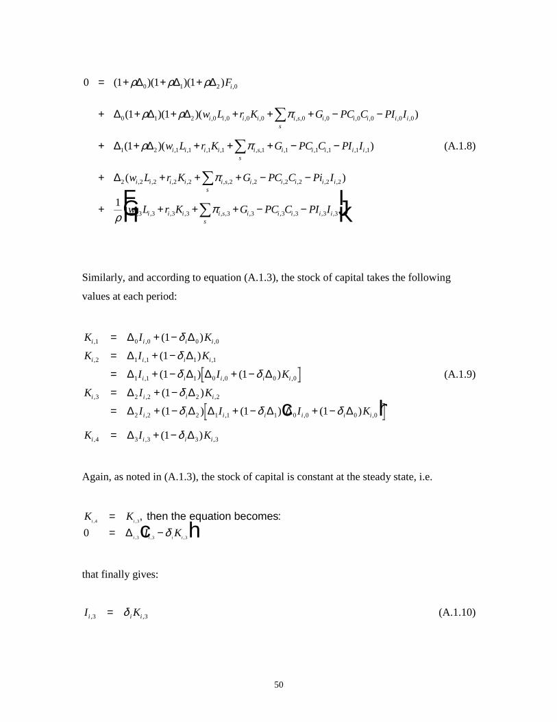
Appendix

A.1 Derivation of the Intertemporal Decision Problem

αγ

αρ γ

γ γ

v vi v V

v

Vi VC C

∆ , ,

( ) ( )

11

0

1 1

1 1

−−

=

− −

−+

−� (A.1.1)

subject to:

F F F w L r K G PC C PI I

F F

i v i v v i v i v i v i v i v i s vs

i v i v i v i v i v

i V i V

, , , , , , , , , , , , , ,

, ,

;+

−

− = + + + + − −LNM

OQP

=

�1

1

∆ ρ π

with (A.1.2)

K K I KK K

i v i v v i v i i v

i V i V

, , , ,

, ,

;+

−

− = −=

1

1

∆ δwith (A.1.3)

In order to clarify the exposition, we first assume that V=3 (i.e. 3 aggregate time periods).

According to equation (A.1.2), the stock of foreign assets takes the following values at

each period of time:

F F w L r K G PC C PI Ii i i i i i i ss

i i i i i, , , , , , , , , , , , ,( ) ( )1 0 0 0 0 0 0 0 0 0 0 0 0 01= + + + + + − −�ρ π∆ ∆ (A.1.4)

F F w L r K G PC C PI I

F

w L r K G PC C PI I

w L r K G

i i i i i i i ss

i i i i i

i

i i i i i ss

i i i i i

i i i i i ss

, , , , , , , , , , , , ,

,

, , , , , , , , , , ,

, , , , , ,

( ) ( )

( )( )

( )( )

(

2 1 1 1 1 1 1 1 1 1 1 1 1 1

0 1 0

0 1 0 0 0 0 0 0 0 0 0 0

1 1 1 1 1 1

1

1 1

1

= + + + + + − −

= + +

+ + + + + − −

+ + + +

�

�

�

ρ π

ρ ρ

ρ π

π

∆ ∆

∆ ∆

∆ ∆

∆

i i i i iPC C PI I, , , , , )1 1 1 1 1− −

(A.1.5)

49

F F w L r K G PC C PI I

F

w L r K G PC C PI I

w L r

i i i i i i i ss

i i i i i

i

i i i i i ss

i i i i i

i i i

, , , , , , , , , , , , ,

,

, , , , , , , , , , ,

, ,

( ) ( )

( )( )( )

( )( )( )

( )(

3 2 2 2 2 2 2 2 2 2 2 2 2 2

0 1 2 0

0 1 2 0 0 0 0 0 0 0 0 0 0

1 2 1 1

1

1 1 1

1 1

1

= + + + + + − −

= + + +

+ + + + + + − −

+ + +

�

�

ρ π

ρ ρ ρ

ρ ρ π

ρ

∆ ∆

∆ ∆ ∆

∆ ∆ ∆

∆ ∆ , , , , , , , , ,

, , , , , , , , , , ,

)

( )

1 1 1 1 1 1 1 1

2 2 2 2 2 2 2 2 2 2 2

K G PC C PI I

w L r K G PC C PI I

i i ss

i i i i i

i i i i i ss

i i i i i

+ + − −

+ + + + − −

�

�

π

π∆

(A.1.6)

F F w L r K G PC C PI Ii i i i i i i ss

i i i i i, , , , , , , , , , , , ,( ) ( )4 3 3 3 3 3 3 3 3 3 3 3 3 31= + + + + + − −�ρ π∆ ∆

As noted in (A.1.2), the stock of foreign assets is constant in steady state, i.e.:

F Fi i, ,4 3=

Therefore, the previous equation becomes:

0 3 3 3 3 3 3 3 3 3 3 3= + + + + − −�ρ πF w L r K G PC C PI Ii i i i i i s i i i i is

, , , , , , , , , , , , ,

which implies:

F PC C PI I w L r K Gi i i i i i i i i i ss

i, , , , , , , , , , , ,3 3 3 3 3 3 3 3 3 3 31= + − − − −FHG

IKJ�ρ

π (A.1.7)

Substituting (A.1.7) into (A.1.6), the constraint (A.1.2) can be rewritten as:

50

0 1 1 1

1 1

1

0 1 2 0

0 1 2 0 0 0 0 0 0 0 0 0 0

1 2 1 1 1 1 1 1 1 1 1 1

2 2 2 2 2 2

= + + +

+ + + + + + − −

+ + + + + − −

+ + +

�

�

�

( )( )( )

( )( )( )

( )( )

(

,

, , , , , , , , , , ,

, , , , , , , , , , ,

, , , , , ,

ρ ρ ρ

ρ ρ π

ρ π

π

∆ ∆ ∆

∆ ∆ ∆

∆ ∆

∆

F

w L r K G PC C PI I

w L r K G PC C PI I

w L r K

i

i i i i i ss

i i i i i

i i i i i ss

i i i i i

i i i i i ss

+ − −

+ + + + − −FHG

IKJ�

G PC C Pi I

w L r K G PC C PI I

i i i i i

i i i i i ss

i i i i i

, , , , ,

, , , , , , , , , , ,

)2 2 2 2 2

3 3 3 3 3 3 3 3 3 31ρ

π

(A.1.8)

Similarly, and according to equation (A.1.3), the stock of capital takes the following

values at each period:

K I K

K I K

I I K

K I K

I I I K

i i i i

i i i i

i i i i i

i i i i

i i i i i i i

, , ,

, , ,

, , ,

, , ,

, , , ,

( )

( )

( ) ( )

( )

( ) ( ) ( )

1 0 0 0 0

2 1 1 1 1

1 1 1 0 0 0 0

3 2 2 2 2

2 2 2 1 1 1 0 0 0 0

1

1

1 1

1

1 1 1

= + −

= + −

= + − + −

= + −

= + − + − + −

∆ ∆

∆ ∆

∆ ∆ ∆ ∆

∆ ∆

∆ ∆ ∆ ∆ ∆ ∆

δδδ δδδ δ δc h

(A.1.9)

K I Ki i i i, , ,( )4 3 3 3 31= + −∆ ∆δ

Again, as noted in (A.1.3), the stock of capital is constant at the steady state, i.e.

K KI K

i i

i i i i

, ,

, , ,

4 3

3 3 30== −

, then the :equation becomes∆ δc h

that finally gives:

I Ki i i, ,3 3= δ (A.1.10)

51

Substituting these values of the stock of capital at each period (A.1.10), as well as

(A.1.9), into the constraint (A.1.8) yields the following new general constraint of the

problem:

0 1 1 1

1 1

1 1

0 1 2 0

0 1 2 0 0 0 0 0 0 0 0 0 0

1 2 1 1 1 0 0 0 0 1 1 1 1 1 1

2 2

= + + +

+ + + + + + − −

+ + + + − + + − −LNM

OQP

+

�

�

( )( )( )

( )( )( )

( )

,

, , , , , , , , , , ,

, , , , , , , , , , , ,

,

ρ ρ ρ

ρ ρ π

ρ δ π

∆ ∆ ∆

∆ ∆ ∆

∆ ∆ ∆ ∆

∆

F

w L r K G PC C PI I

w L r I K G PC C PI I

w L

i

i i i i i ss

i i i i i

i i i i i i i ss

i i i i i

i

b gm ri i i i i i i i s

si i i i i

i ii

ii i i s

si i i

r I I K G PC C Pi I

w Lr

PI I G PC C

, , , , , , , , , , , ,

, ,,

, , , , , , ,

2 2 1 1 1 0 0 0 0 2 2 2 2 2 2

3 33

3 3 3 3 3 3

1 1

1

+ + − + − + + − −LNM

OQP

+ + −FHG

IKJ + + −

LNM

OQP

�

�

∆ ∆ ∆ ∆δ δ π

ρ δπ

b g b gc hn s(A.1.11)

With V=3, the problem thus consists of maximising:

∆ ∆∆

∆∆ ∆ ∆ ∆0

01

11

1

12

21

1 2

31

1 21 1 1 1 1 1 1 1 1C C C Ci i i i, , , ,

( ) ( )( ) ( )( )( ) ( )( )( )

− − − −

−+

− ++

− + ++

− + +

γ γ γ γ

γ γ ρ γ ρ ρ γ ρ ρ ρ

with respect to Ci,v and Ii,v, subject to the general constraint (A.1.11). Solving this

problem yields the following first order conditions:

∆ ∆ ∆ ∆0 0 2 1 0 01 1C PCi i, ,( )( )− = + +γ λ ρ ρ (A.1.12)

∆ ∆ ∆ ∆1 1 2 1 1 11 1C PCi i, ,( )( )− = + +γ λ ρ ρ (A.1.13)

∆ ∆ ∆ ∆2 2 2 1 2 21 1C PCi i, ,( )( )− = + +γ λ ρ ρ (A.1.14)

∆ ∆ ∆ ∆3 3 2 1 3 31 1C PCi i, ,( )( )− = + +γ λ ρ ρ (A.1.15)

52

( )( ) ( ) ( ) ( )

( ) ( )

( )

. , ,

, ,

, ,

1 1 1 1

1

1

2 1 0 0 2 1 1 0 2 2 1 0

2 1 1 2 2 1

2 3 3

+ + = + + −

+ =

= −

ρ ρ ρ δ

ρ

ρδ

∆ ∆ ∆ ∆ ∆ ∆ ∆ ∆ ∆

∆ ∆ ∆ ∆

PI r r

PI r

PI r PI

i i i i

i i

i i

A

A.1.

A.1

.1.16

17

.18c h

where λ is the Lagrange multiplier. By combining equations (A.1.12) to (A.1.15), we

obtain:

CC

PCPC

i

i

i

i

,

,

,

,

0

1

0

1

−

− =γ

γ ,

CC

PCPC

i

i

i

i

,

,

,

,

2

3

2

3

−

− =γ

γ ,

and by combining equations (A.1.16) to (A.1.18), we get:

PI r PI

PI r PI

i i i i

i i

, , ,

, ,

( )

.

01

1 1 1 1

2 3 3

11

1

1

=+

+ −

= −

ρδ

ρδ

∆∆ ∆

and:

c h

A.2 Derivation of the Expenditure Allocation Across Commodities

Maxc i s v i s v

si s v

i sU c c, ,

,( ), , , , = ∏ ρ (A.2.1)

subject to:

PC C Pc ci v i v i s v i s vs

i ss

, , , , , ,

,

=

=

�

�

(A .2.2)

(A .2.3)ρ 1

53

The first-order condition for a given good s takes the following form:

ρ λρ ρi s i s v i w v

w si s vc c Pci s i w

, , , , , , ,, ,−

≠∏ =1

Multiplying both sides by ci s v, , :

ρ λρi s i s v

si s v i s vc Pc ci s

, , , , , , ,,∏ = . (A.2.4)

Taking the sum over all goods gives:

c Pc ci s vs

i ss

i s v i s vs

i s, , , , , , ,

,ρ ρ λ∏ � �= .

Substituting constraints (A.2.2) and (A.2.3) in the above equation, and given that

c Ci s vs

i vi s

, , ,,ρ∏ =

yields the following explicit form for the Lagrange multiplier:

C PC CPCi v i v i v

i v, , ,

,

= � =λ λ 1 .

Replacing λ by its value in (A.2.3) gives the final consumption demand of therepresentative household of country i for good s at period v

cPC C

Pci s v i si v i v

i s v, , ,

, ,

, ,

= ρ , (A.2.5)

where the aggregate price PCi,v is derived by first using the constraint (A.2.2):

54

PCPc c

Ci v

i s v i s vs

i v,

, , , ,

,

=�

Then, using the objective function (A.2.1) and (A.2.4):

PCPC C

PC CPc

i vi v i v

i s i v i v

i s vs

i s,, ,

, , ,

, ,

,= F

HGIKJ∏ ρ

ρ ,

which can be rewritten as:

PCPC C

PC CPc

i vi v i v

i v i vi s

i s vs

i ss

i s,, ,

, ,,

, ,

,

,=

� FHG

IKJ∏c hρ

ρρ

,

to finally get:

PCPc

i vi s v

i ss

i s

,, ,

,

,

=FHG

IKJ∏ ρ

ρ

A.3 Geographical Origins of Consumption and Investment goods

Max c

c s

c sc i s v

j i s j i s vj

j i s j i s vfj

j i s v

c s i

c s i

c s i

c s i

cf s i

cf s i

cf s i

cf s i

f f

, , ,

, ,

, ,

, ,

, ,

, ,

, ,

, ,

, ,, ,

, , , , ,

, , , , , , ,

,

,

if is produced in a competitive sector

if is produced in a non-competitive sector,

=

LNMM

OQPP

LNMM

OQPP

R

S

||||

T

||||

− −

− −

�

��

δ

δ

σσ

σσ

σ

σ

σ

σ

1 1

1 1 (A.3.1)

55

subject to:

Pc c

P c s

P c si s v i s v

j i s v j i s v j i s vj

j i s v j f i s v j f i s vfj

, , , ,

, , , , , , , , ,

, , , , , , , , , , ,

( ) ,

( ) ,=

+

+

RS||T||�

��

1

1

τ

τ

if is competitive

if is non - competitive,

yields

δ δ λ τσσ

σσ σ

σj i s j i s v

jk i s k i s v k i s v k i s vc c P

c s i

c s i

c s i

c s i c s i

c s i, , , , , , , , , , , , , , , ,

, ,

, ,

, ,

, , , ,

, ,

− −− −

−

�LNMM

OQPP = +

1 11 1

1

1c h . (A.3.2)

By multiplying both sides of equation (A.3.2) by ck i s v, , , , we have:

δ δ λ τσσ

σ σσ

j i s j i s vj

k i s k i s v k i s v k i s v k i s vc c P cc s i

c s i

c s i c s i

c s i, , , , , , , , , , , , , , , , , , ,

, ,

, ,

, , , ,

, , ( )− − −

�LNMM

OQPP = +

11

1 1

1 . (A.3.3)

A similar first-order condition exists for each geographical origin. Taking the sum over

all geographical origins gives:

δ δ λ τσσ

σ σσ

j i s j i s vj

k i s k i s vk

k i s v k i s v k i s vk

c c P cc s i

c s i

c s i c i s

c i s, , , , , , , , , , , , , , , , , , ,

, ,

, ,

, , , ,

, , ( )− − −

� � �LNMM

OQPP

LNMM

OQPP= +

11

1 1

1 ,

or:

c P ci s v k i s v k i s v k i s vk

, , , , , , , , , , ,( )= +�λ τ1 .

56

Using constraint (A.3.2) in the above equation yields an explicit expression for the

Lagrange multiplier:

c Pc cPci s v i s v i s v

i s v, , , , , ,

, ,

= � =λ λ 1 .

Replacing λ in (A.3.3) by the above relationship yields the following demand function

for good s produced by a competitive sector in country k:

c P Pc ck i s v k i s k i s v k i s v i s v i s vc i s c i s c i s

, , , , , , , , , , , , , , ,, , , , , ,( )= +

−δ τσ σ σ1 (A.3.4)

Combining (A.3.4) with the constraint (A.3.2) gives the explicit form of the aggregate

price Pci s v, , :

PcP c

c

Pc c P

c

P

i s v

j i s v j i s v j i s vj

i s v

i s v i s v j i s j i s v j i s vj

i s v

j i s j i s v j i s vj

c s i c s i c s i

c s i c s i c s i

, ,

, , , , , , , , ,

, ,

, , , , , , , , , , , ,

, ,

, , , , , , , ,

( )

( )

( ) .

, , , , , ,

, , , , , ,

=+

=+

= +LNM

OQP

�

�

�

−

− −

1

1

1

1

1

11

τ

δ τ

δ τ

σ σ σ

σ σ σ

d i

d i

The first-order conditions for a given good produced by a non-competitive firm f of

sector s in country k, takes the following form:

δ δ λ τσ

σ

σ

σ σ

σj i s j i s v

fjk i s k i s v k i s v k i s vf f f f f

c c Pc f s i

c f s i

c f s i

c f s i c f i s

c f i s

, , , , , , , , , , , , , , , , , , , , ,

, ,

, ,

, ,

, , , ,

, , ( )

− −− −

−

��LNMM

OQPP = +

1 11 1

1

1 (A.3.6)

Taking the same steps that we have taken for the competitive sector yields the following

demand function:

57

c P Pc ck f i s v k f i s k i s v k f i s v i s v i s vc f i s c f i s c f i s

, , , , , , , , , , , , , , , , , ,, , , , , ,( )= +

−δ τσ σ σ1

. (A.3.7)

The aggregate price Pci s v, , is given by combining (A.3.7) with (A.3.2):

PcP c

c

Pc c P

c

P

i s v

j i s v j f i s v j f i s vfj

i s v

i s v i s v j f i s j i s v j f i s vfj

i s v

j f i s j i s v j f i s vfj

c f i s c f i s c f i s

c f i s c f i s

, ,

, , , , , , , , , , ,

, ,

, , , , , , , , , , , , , ,

, ,

, , , , , , , , , ,

( )

( )

( )

, , , , , ,

, , , ,

=+

=+

= +L

��

��

��

−

−

1

1

1

1

1

τ

δ τ

δ τ

σ σ σ

σ σ

d i

d iNMOQP

−1

1 σ c f i s, ,

.

(A.3.8)

Firms in non-competitive industries are assumed to be symmetric within national

boundaries. This symmetry assumption implies that imperfectly competitive domestic

firms within a sector have the same cost structure and market share. Consequently, they

will charge the same price even though the goods are imperfect substitutes from the

users’ point of view. Equations (A.3.7) and (A.3.8) can thus be rewritten:

c P Pc ck f i s v k f i s k i s v k i s v i s v i s vc f i s c f i s c f i s

, , , , , , , , , , , , , , , , ,, , , , , ,( )= +

−δ τσ σ σ1 ,

Pc n Pi s v j s v j f i s j i s v j i s vj

c f i s c f i s c f i s

, , , , , , , , , , , , ,, , , , , ,

( )= +LNM

OQP

− −

� δ τσ σ σ

11

11d i

A.4 Bertrand Elasticities

Deriving the consumption demand function (3.2.1.6) with respect to its own price yields:

58

∂

∂ += − + +L

NMOQP

− − +

− − −−

�c

PP n P Pc ci j s v

i j s v i j s vc j s i j s i j s v i j s v i s v i j s i j s v i j s v

ij s v j s v

c j s i j s

f

f ff

cf j s cf j s cf j s cf j s

f

, , , ,

, , , , , ,, , , , , , , , , , , , , , , , , , , , , , , , , ,

, , , ,

( )( ) ( )

( ) (

, , , , , , , ,

11 1

1 1

1 11

τσ δ τ δ τ

σ τ

σ σ σ σd i, , , , , , , , , , , , , , , ,

, , , , , , , , , , , , , , ,

, , , , ,

) ( )

( )

(

, , , , , , , ,

, , , ,

, ,

v i j s v i j s i j s i j s v i j s v

i s v i j s i j s v i j s vi

j s v j s v

c j s i j s

P P

n P Pc C

cf j s cf j s cf j s cf j s

cf j s cf j s

f

cf j s

f f

f

f

− −

−−

+

• +LNM

OQP

= − +

�

σ σ σ σ

σ σ

σ

δ δ τ

δ τ

σ δ τ

1

1

1

12

d ii j s v i j s v i s v i j s i j s v i j s v

ij s v j s v

c j s i j s v i j s v i j s i j s i j s v

P n P Pc c

P

cf j s cf j s cf j s

f

cf j s cf j s

f

cf j s

f

f

, , , , , , , , , , , , , , , , , , , , ,

, , , , , , , , , , , , , , , ,

) ( )

( ) ( ) ( )

, , , , , ,

, , , , , ,

− − −−

−

+LNM

OQP

− − + +

�σ σ σ

σ σ σ

δ τ

σ τ δ δ τ

1 11

1

1 1 1

d iP

n P n P Pc c

i j s v

i s v i j s i j s v i j s vi

i s v i j s i j s v i j s vi

j s v j s v

cf j s

cf j s cf j s cf j s cf j s

f f

, , ,

, , , , , , , , , , , , , , , , , , , , , , , , , ,

, ,

, , , , , , , ,( ) ( )

−

−−

−−

• +LNM

OQP +LNM

OQP� �

σ

σ σ σ σδ τ δ τ 1 1

11

11

d i d i

Since:

n P Pci s v i j s i j s v i j s vi

j s vf

c f j s c f j s c f j s

, , , , , , , , , , , , ,, , , , , ,( )δ τσ σ σ1

11

1+LNM

OQP=

−−

−� d i ,

then:

59

∂

∂ += − + +

− − +

− − −c

PP P Pc c

i j s v

i j s v i j s vc j s i j s i j s v i j s v i j s v i j s v j s v j s v

c j s i j s i j s i j

f

f f

f f

cf j s cf j s cf j s

f

c f j s cf j s

, , , ,

, , , , , ,, , , , , , , , , , , , , , , , , , , ,

, , , , , , , , ,

( )( ) ( )

( ) (

, , , , , ,

, , , ,

11 1

1 1

1 1

τσ δ τ τ

σ δ δ τ

σ σ σ

σ σ

d i d i d i, , , , ,

, , , , , , , , , , , , , ,

, , , , , , , , , , , , , , , , , ,

)

( )

( )

, ,

, , , , , ,

, , , , , ,

s v i j s v

i j s v i j s v j s v j s v j s v j s v

i j s i j s v i j s v i j s v j s v j s v j s v

c

P

P Pc Pc Pc c

P Pc Pc c

cf j s

cf j s cf i s cf j s

cf j s cf j s cf j s

f

d id i

d i

−

− − −

− −

• +

= +

• −

σ

σ σ σ

σ σ σ

τ

δ τ

σ

1

1

1 1

1

f f

c f j s c f j s c f j s

f f

f

j s i j s v i j s v c j s i j s i j s v i j s v j s v

i j s v c j s i j s v i j s v c j si j s v

j s v j s v

P P Pc

c Pc

Pc c

f

f

, , , , , , , , , , , , , , , , , , , , ,

, , , , , , , , , , , , , ,, , ,

, , , ,

( ) ( ) ( )

( ) ( )

, , , , , ,1 1 1

1 1

1 1

1

+ − − +

− + − −LNMM

− − −

−

τ σ δ τ

σ τ σ

σ σ σd i d id i=

OQPP

Therefore, using (3.2.1.4), the Bertrand direct price elasticity for the consumption

demand follows:

ε σ στ

( , ) ( )( )

, , , , , , , , , , ,, , , , , , , , , ,

, , , ,

c PP c

Pc ci j s v i j s v c j s c j si j s v i j s v i j s v

j s v j s vf

f

f f= − − −

+1

1d i .

A.4 Cournot Elasticities

Max P q v q w L r Kq i j s v i f j s v i f j s v i s v i f j s v

ji v i f s i v i f s

i f j s vff

, , , ,, , , , , , , , , , , , , , , , , , , , , , , ,

j

π = − − −� � (A.4.1)

subject to:

q c i xi f j s v i f j s v i f j s v i f j s sd vsd

, , , , , , , , , , , , , , , , ,= + +� (A.4.2)

solving

qPq

P vi f j s vi f j s v

i f j s vi f j s v i f s v, , , ,

, , , ,

, , , ,, , , , , , ,

∂∂

+ = . (A.4.3)

60

Dividing by Pi,f,j,s yields:

ε

ε

( , )

( , )

, , , , , , , ,, , ,

, , , ,

, , , , , , , , , , , , , , ,

P qvP

P P q v

i f j s v i f j s vi f s v

i f j s v

i f j s v i f j s v i f j s v i f s v

or:

+ =

+ =

1

1d i

dQQP

dPQP

dPQP

dPi f ji f j

i f ji j

i f j

i h jh fi h j

i f j

k h jhk ik h jf, ,

, ,

, ,,

, ,

, ,, ,

, ,

, ,, ,=

∂∂

+∂∂

+∂∂≠ ≠

� ��

After rearranging, we get:

dQQ

Q PdPP

Q PdPP

Q PdPP

j

jj k j

h

n

k

K k j

k j

j k jh

n

k

K k j

k j

j k jh

n

k

K k j

k j

hh

h

hh

h

n hh

h

k

k

k

1,1

1,11,1

1,2

1

11

11

11

0

01

,

,, , ,

, ,

, ,

, , ,, ,

, ,

, , , ,, ,

, ,

( , )

( , )

( , )

= ��

= ��

= ��

==

==

==

ε

ε

ε

� � �

0

0

2 1

2

11

11 2

= ��

= ��

==

==

ε

ε

( , )

( , )

, , , ,, ,

, ,

, , , ,, ,

, ,

Q PdPP

Q PdPP

j k jh

n

k

K k j

k j

j k jh

n

k

K k j

k j

hh

h

n hh

h

k

k

� � �

61

0

0

111

11

= ��

= ��

==

==

ε

ε

( , )

( , ) .

, , , ,, ,

, ,

, , , ,, ,

, ,

Q PdPP

Q PdPP

K hh

h

K n hh

h

j k jh

n

k

K k j

k j

j k jh

n

k

K k j

k j

k

k

k

� � �

Dividing right and left sides of the equations by dQQ

j

j

1,1

1,1

,

,

gives:

1

0

0

1 1 1 1

1 1 1

1 1 1

11

211

11 1

= ��

= ��

= ��

==

==

==

ε ε

ε ε

ε ε

( , ) ( , )

( , ) ( , )

( , ) ( , )

, , , , , , , ,

, , , , , , , ,

, , , , , , , ,

Q P P Q

Q P P Q

Q P P Q

j k jh

n

k

K

k j j

j k jh

n

k

K

k j j

j k jh

n

k

K

k j j

h h

h h

n h h

k

k

k

� � �

0

0

2 1 1 1

2 1 1

11

11 2

= ��

= ��

==

==

ε ε

ε ε

( , ) ( , )

( , ) ( , )

, , , , , , , ,

, , , , , , , ,

Q P P Q

Q P P Q

j k jh

n

k

K

k j j

j k jh

n

k

K

k j j

h h

n h h

k

k

� � �

0

0

1 1 1

1 1

11

11

= ��

= ��

==

==

ε ε

ε ε

( , ) ( , )

( , ) ( , ),

, , , , , , , ,

, , , , , , , ,

Q P P Q

Q P P Q

K h h

K n h h

j k jh

n

k

K

k j j

j k jh

n

k

K

k j j

k

k

k

� � �

whereε ε( , ) ( , ), , , , , , , ,Q P P Qi j k j k j i jf h h f and are respectively Bertrand and Cournot cross-

price elasticities.

62

The equilibrium computation requires solving one such system for each firm from all

countries k in all markets j. The calculation cost is prohibitive unless the symmetry

assumption between domestic firms is imposed. With this assumption, the system solved

by firm 1 of country 1 becomes:

1

0

0

1 1 1 1

1 2 1 1

1 1 1

1

1

1 1

= �

= �

= �

=

=

=

n Q P P Q

n Q P P Q

n Q P P Q

k j k j k j jk

K

k j k j k j jk

K

k j k j k j jk

K

n

ε ε

ε ε

ε ε

( , ) ( , )

( , ) ( , )

( , ) ( , )

, , , , , ,

, , , , , ,

, , , , , ,

� � �

0

0

2 1 1 1

2 1 1

1

1 2

= �

= �

=

=

n Q P P Q

n Q P P Q

k j k j k j jk

K

k j k j k j jk

K

n

ε ε

ε ε

( , ) ( , )

( , ) ( , )

, , , , , ,

, , , , , ,

� � �

0

0

1 1 1

1 1

1

1

= �

= �

=

=

n Q P P Q

n Q P P Q

k j k j k j jk

K

k j k j k j jk

K

K

K nk

ε ε

ε ε

( , ) ( , )

( , ) ( , )

, , , , , ,

, , , , , ,

� � �

Since all firms of country 1 are symmetric, every firm in that country solves a similar

system. Therefore, the second index relative to a specific firm of each country can be

dismissed. Let us rewrite the system as follows:

63

1 1

0 1

1,1 1, 1, 1 1 1,1 1 1 1 1 1 1 1 1

1,2 1, 1, 1 1 1,2 1 1 1 1 1,2 1

11

1

= + − +

= + − +≠�ε ε ε ε ε ε

ε ε ε ε ε ε

( , ) ( , ) ( ) ( , ) ( , ) ( , ) ( , )

( , ) ( , ) ( ) ( , ) ( , ) ( , ) ( ,

, , , , , , , , , , , , , ,

, , , , , , , , , , ,

Q P P Q n Q P P Q n Q P P Q

Q P P Q n Q P P Q n Q P P Q

j j j j j j j j k j k j k j jk

j j j j j j j j k j k j k j , ,

, , , , , , , , , , , , , ,

)

( , ) ( , ) ( ) ( , ) ( , ) ( , ) ( , )

1

1, 1, 1, 1 1 1, 1 1 1 1 1 1 1

1

11

0 11 1 1

jk

j j j j j j j j k j k j k j jk

Q P P Q n Q P P Q n Q P P Qn n n

≠

≠

�

�= + − +

� � �

ε ε ε ε ε ε

0 1

0 1

2 1, 1, 1 1 2 1 1 1 1 2 1 1 1

1, 1, 1, 1 1 2 1 1 1 1 2

22

22 2 2

= + − +

= + − +

≠�ε ε ε ε ε ε

ε ε ε ε ε

( , ) ( , ) ( ) ( , ) ( , ) ( , ) ( , )

( , ) ( , ) ( ) ( , ) ( , ) ( , )

,1 ,1

, ,

, , , , , , , , , , , , , ,

, , , , , , , , , ,

Q P P Q n Q P P Q n Q P P Q

Q P P Q n Q P P Q n Q P

j j j j j j j j k j k j k j jk

j j j j j j j j k j k jn n n

� � �

ε( , ), , ,P Qk j jk

1 12≠�

0 1

0 1

2 1, 1, 1 1 2 1 1 1 1 2 1 1 1

1, 1, 1, 1 1 2 1 1 1 1 2

22

22 2 2

= + − +

= + − +

≠�ε ε ε ε ε ε

ε ε ε ε ε

( , ) ( , ) ( ) ( , ) ( , ) ( , ) ( , )

( , ) ( , ) ( ) ( , ) ( , ) ( , )

,1 ,1

, ,

, , , , , , , , , , , , , ,

, , , , , , , , , ,

Q P P Q n Q P P Q n Q P P Q

Q P P Q n Q P P Q n Q P

j j j j j j j j k j k j k j jk

j j j j j j j j k j k jn n n

� � �

ε( , ), , ,P Qk j jk

1 12≠�

This square system of nkk

K

=�

1

equations can be simplified further. As shown by equations

(3.2.1.7) and (3.2.1.8), a simple relationship links Bertrand direct and cross-price

elasticitities:

ε ε σ( , ) ( , ), , , , , , , ,Q P Q Pi j i j k j i j jf f h f= − . (3.2.2.7)

It can be demonstrated that a similar relationship between Cournot direct and cross-price

elasticities can be derived:

ε εσ

( , ) ( , ), , , , , , , ,P Q P Qi j i j k j i jj

f f h f= − 1 .

Using these two relationships, the system for the firms of country 1 can be rewritten as:

64

1 1 1

0 1 2

1,2 1, 1, 11 1,1 1 1 11 11 11

1,2 1, 1, 11 1,2 1, 1, 11 1,2 1

11

1

= − − + − +

= − + − + −≠�ε σ ε σ ε ε ε ε

ε ε σ ε σ ε ε

( , ) ( , ) ( ) ( , ) ( , ) ( , ) ( , )

( , ) ( , ) ( , ) ( , ) ( ) ( ,

, , , , , , , , , , , , , ,

, , , , , , , ,

Q P P Q n Q P P Q n Q P P Q

Q P P Q Q P P Q n Q P

j j j j j j j j j j k j k j k j jk

j j j j j j j j j j j j j j k j k j k j jk

j j j j j j j j j j j j j j k j k j k j j

P Q n Q P P Q

Q P P Q Q P P Q n Q P P Q n Q P P Qn n n n

) ( , ) ( , ) ( , )

( , ) ( , ) ( , ) ( , ) ( ) ( , ) ( , ) ( , ) ( ,

, , , , , , , ,

, , , , , , , , , , , , , , , , ,

ε ε ε

ε ε σ ε σ ε ε ε ε ε

1 11 1,2 11

1, 1, 1, 11 1, 1, 1, 11 1, 1 1 11 1 11

1

10 1 21 1 1 1

+

= − + − + − +

≠�

� � �

)k≠�

1

0 1 2

0 1

2 1, 2 11 2 1, 2 11 2 1 1 11 2 1 11

2 1, 2 11 2 1,

22

2 2

= − + − + − +

= − +

≠�ε ε σ ε σ ε ε ε ε ε

ε ε σ ε

( , ) ( , ) ( , ) ( , ) ( ) ( , ) ( , ) ( , ) ( , )

( , ) ( , ) ( ,

,1 , ,1 , ,1

, , ,

, , , , , , , , , , , , , , , , ,

, , , ,

Q P P Q Q P P Q n Q P P Q n Q P P Q

Q P P Q Q P

j j j j j j j j j j j j j j k j k j k j jk

j j j j j jn n

� � �

j j j j j j j j k j k j k j jk

P Q n Q P P Q n Q P P Qn n) ( , ) ( ) ( , ) ( , ) ( , ) ( , ), , ,, , , , , , , , , , , ,− + − +≠�σ ε ε ε ε ε2 11 2 1 1 11 2 112

2

22 2

�

0 1 2

0 1

1, 11 1, 11 1 1 11 21 11

1, 11

= − + − + − +

= − +

≠�ε ε σ ε σ ε ε ε ε ε

ε ε σ ε

( , ) ( , ) ( , ) ( , ) ( ) ( , ) ( , ) ( , ) ( , )

( , ) ( , ) ( ,

,1 , ,1 , ,

, , ,

, , , , , , , , , , , , , , , , ,

, , , ,

Q P P Q Q P P Q n Q P P Q n Q P P Q

Q P P Q Q

K K K K Kn

Kn K Kn

j j j j j j j j j j K j j j j k j k j k j jk K

j j j j j j

k

k k

� � �

P P Q n Q P P Q n Q P P Qj j j j K j j j j k j k j k j jk K

K Kn nk1, 11 1 1 11 2 1122

) ( , ) ( ) ( , ) ( , ) ( , ) ( , ), , ,, , , , , , , , , , , ,− + − +≠�σ ε ε ε ε ε

Given the relationship between Cournot own and cross-price elasticities, only cross

elasticities remain in the system, that is nkk

K

=� −FHG

IKJ1

1 variables. One of the equations of the

system is therefore redundant and can be dropped. Dropping the first equation out of the

demand system, and rearranging we have:

0 1 1

0 1 1

1,2 1, 1, 1 1 1, 11 1,2 1 1 1 1 1,2 1 1

1, 1, 1, 1 1 1, 11 1,

11

11 1

= − − + − +

= − − + −

≠�ε ε σ σ ε ε ε ε ε

ε ε σ σ ε ε

( , ) ( , ) ( , ) ( ) ( , ) ( , ) ( , ) ( , )

( , ) ( , ) ( , ) ( ) (

, , , , , , , , , , , , , , ,

, , , , , ,

Q P P Q P Q n Q P P Q n Q P P Q

Q P P Q P Q n Q

j j j j j j j j j j j j k j k j k j jk

j j j j j j j jn n

� � �

j j j j k j k j k j jk

P P Q n Q P P Qn, ) ( , ) ( , ) ( , ), , , , , , , , , ,1 1 1 1 1 1 11

1

ε ε ε+≠�

�

65

0 1 1

0 1 1

2 1, 2 1 1 2 1 1 2 1 1 11 2 1 11

2 1, 2 1 1 2 11

22

22

= − − + − +

= − − + −

≠�ε ε σ σ ε ε ε ε ε

ε ε σ σ ε ε

( , ) ( , ) ( , ) ( ) ( , ) ( , ) ( , ) ( , )

( , ) ( , ) ( , ) ( ) (

,1 , , ,1

, , ,

, , , , , , , , , , , , , , , ,

, , , , ,

Q P P Q P Q n Q P P Q n Q P P Q

Q P P Q P Q n

j j j j j j j j j j j j k j k j k j jk

j j j j j j j jn

� � �

Q P P Q n Q P P Qn nj j j j k j k j k j jk

2 1 1 1 1 2 1 12 2

2, ,, , , , , , , , , ,, ) ( , ) ( , ) ( , )ε ε ε+

≠�

�

0 1 1

0 1 1

1, 11 11 1 1 11 2 1 11

1, 11 11

= − − + − +

= − − + −

≠�ε ε σ σ ε ε ε ε ε

ε ε σ σ ε

( , ) ( , ) ( , ) ( ) ( , ) ( , ) ( , ) ( , )

( , ) ( , ) ( , ) ( )

,1 , , ,

, , ,

, , , , , , , , , , , , , , , ,

, , , , ,

Q P P Q P Q n Q P P Q n Q P P Q

Q P P Q P Q n

K K K K n

K n K K

j j j j j j j j K j j j j k j k j k j jk K

j j j j j j j j K

k

k

� � �

ε ε ε ε( , ) ( , ) ( , ) ( , ), ,, , , , , , , , , ,Q P P Q n Q P P QK n nk j j j j k j k j k j jk K

1 1 11 2 112+

≠�

Given that all non-competitive firms of a given country i are identical (the symmetryassumption), this system can finally be written in a more compact form:

0 1

1 210

1=

where: , , ... , =

( ) ( , ) ( , ) ( , ) ( , ), , , , , , , , , ,

,

,

n Q P P Q Q P P Q

h Kif k iif k i

k k i h j k j h j h j i j h j i j i j i j

i jk

K

k i

− − + −FHG

IKJ

=

=≠

RST

=� δ ε σ ε ε ε

σ

δ

and where ε ε( , ) ( , ), , , , , , , ,Q P P Qi j k j k j i jf h h f and are respectively Bertrand and Cournot

cross-price elasticities.