A MULTI-STAGE HEDONIC MARKET MODEL OF COTTON ...

A MULTI-STAGE HEDONIC MARKET MODEL OF COTTON CHARACTERISTICS

WITH SEPARABLE SUPPLY AND DEMAND

by

KENNETH RAY BOWMAN, B.S., M.S.

A DISSERTATION

IN

AGRICULTURE

Submitted to the Graduate Faculty of Texas Tech University in

Partial Fulfillment of the Requirements for

the Degree of

DOCTOR OF PHILOSOPHY

Approved

May, 1989

ACKNOWLEDGEMENTS

The author would like to express his sincere

appreciation to Dr. Don E. Ethridge for his foresight and

guidance. He would also like to thank Dr. Kary Mathis, Dr.

Sujit K. Roy, Dr. Derald Walling, and Dr. Jack Gipson for

their assistance and patience in completing this project.

Special thanks are due to Dr. Don Smith, Dr. Foy

Mills, Dr. R.T. Ervin, and Dr. W.F. Edwards for their

friendship and moral support. The author also wishes to

thank David McGaughey, Dr. Sherwin Rosen, and Dr. Homer

Erickson for their assistance and comments.

This work was funded by grants from the United States

Department of Agriculture, and the Thornton Institute of

Texas Tech University.

The author also wishes to thank his family members for

their needed encouragement.

11

CONTENTS

ACKNOWLEDGEMENTS ii ABSTRACT v LIST OF TABLES vii

I. INTRODUCTION 1 Price Discovery in Cotton 4 Objectives 7 Overview of Procedures 7

II. REVIEW OF LITERATURE 9 Characteristic Demand Theory 9 Nonagricultural Empirical Studies 13 Noncotton Agricultural Models 23 Cotton Characteristic Pricing Research 27

III. CONCEPTUAL FRAMEWORK 36 The Hedonic Pricing Concept 37 Hedonic Pricing Applied to Cotton 41 A Modified Conceptualization 46 A Model for Cotton 49 Demand Factors 52 Supply Factors 53

IV. METHODS AND PROCEDURES 55 Description of the Data 55 First Stage Hedonic Model 59 An Hedonic Model For Cotton Pricing 63 Variable Explanations and Parameter Expectations 64 Estimation of First Stage Hedonic Price Model 66 A Revised First Stage Discount Model 67 Structural Equations 71 Characteristic Demand (Second Stage) Equations 76 Structural Equations for Characteristic Specific Demand 80 Characteristic Supply (Second Stage) Equations 83 Structural Supply Equations for Cotton Fiber Properties 86 Estimation Procedures 88 Interpretation of Models 91

iii

RESULTS AND ANALYSIS 94 Hedonic Price Discounts 94 Results and Analysis for 1976 96 Results for Other Years 101 Characteristic Price Flexibilities 112 Characteristic Specific Demand Equations 120 Characteristic Specific Supply Equations 135

VI. SUMMARY AND CONCLUSIONS 152 Summary 151 Conclusions 161 Suggestions for Further Research 164

BIBLIOGRAPHY 166

APPENDIX 171

IV

ABSTRACT

This study examined the impacts of fiber

characteristics on cotton prices from 1976 to 1986 for 4

production and marketing regions of the United States. A

set of 11 equations were estimated to determine the effects

of cotton fiber characteristics on cotton prices. Trash,

color, staple length, micronaire, and strength were found

to have statistically significant impacts on cotton

prices. Length uniformity was not statistically

significant. Characteristic effects were found to vary

across time and across regions. However, trends in

attribute values were similar for all characteristics

across all regions. Characteristic price flexibilities

were calculated using the regional base prices and

characteristic averages of each year. Cotton prices were

not price responsive with respect to characteristic

variation. In this context, percentage changes in

characteristic levels did not cause equivalent percentage

changes in cotton prices. A set of 24 equations found that

cotton characteristic values were functions of other

characteristics as well as characteristic specific demand

shifters, base price and proportion of open end spindles to

ring spindles. Characteristic impacts on characteristic

values were similar across regions, though some variation

of effects were present. The effects of base price were

also similar across regions. The proportion of open end

spindles to ring spindles affected characteristic values

with the largest impacts occurring in the West. Separate

systems of equations were constructed to estimate the

effects of environmental variables on each cotton

characteristic in each production region of the country.

Seasonal rainfall and temperature affected characteristics

in all regions though parameter estimates and functional

forms varied considerably among production areas.

There is a growing recognition of the need to

understand the values of fiber characteristics. Fiber

characteristic values affect the revenues of producers and

the costs of buyers. The results of this study demonstrate

that there is a functioning market for cotton

characteristics. The characteristics model constructed in

this paper is useful because it presents an alternative to

the current method of determining fiber quality premiums

and discounts.

VI

LIST OF TABLES

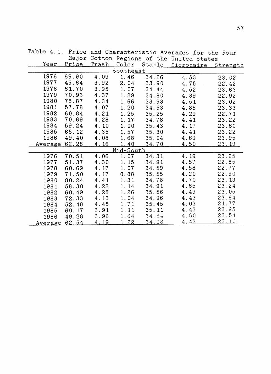
4.1 Price and Characteristic Averages for the Four Major Cotton Production Regions of the United States 57

5.1 Hedonic Discount Equation Results for 1976 97

5.2 Discounts for Cotton Attributes in the Four Major Cotton Production Regions: 1976-1986 102

5.3 Price Flexibilities for Cotton Attributes in the Four Major Production Regions: 1976-1986 114

5.4 Characteristic Specific Demand Equations: Southeast Region 121

5.5 Characteristic Specific Demand Equations: Mid-South Region 123

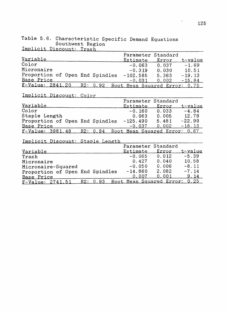
5.6 Characteristic Specific Demand Equations: Southwest Region 125

5.7 Characteristic Specific Demand Equations:

West Region 127

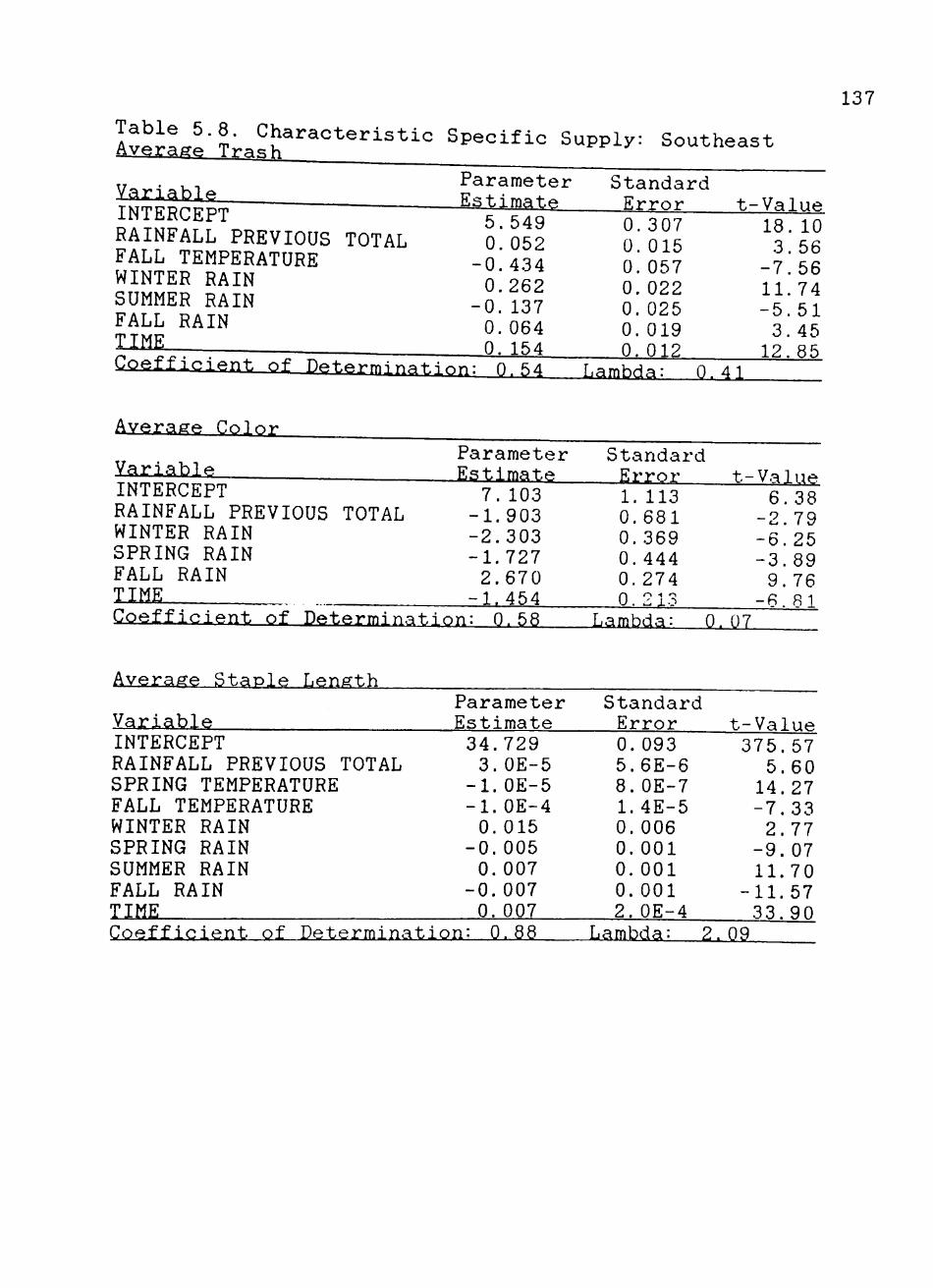
5.8 Characteristic Specific Supply: Southeast 137

5.9 Characteristic Specific Supply: Mid-South 139

5.10 Characteristic Specific Supply: Southwest 141

5. 11 Characteristic Specific Supply: West 143

A.1 Hedonic Discount Results for 1977 172







Vll




Vlll

CHAPTER I

INTRODUCTION

In a market oriented economic system, the price of any

product is determined by the forces of supply and demand.

Although an oversimplification, each producer's supply

schedule is a function of many inputs whose own prices are

determined through market forces. A similar analysis is

true for buyers. The value each consumer places on a

product is a function of the expected utility from the

purchase of the product. This level of utility is again a

function of several factors.

A valuable role of price is to convey information.

Given a market price, the information that it contains will

flow through all markets which are related to the

particular good. If the price of a good rises, producers

take this information as a signal to increase the quantity

of the good supplied. They will also demand more of the

resources that are necessary to produce it. Resource

suppliers will react to this market information by

producing greater quantities of the resources. Information

from price variation increases the efficiency with which an

economy is able to satisfy unlimited human wants with

limited resources. Economic agents in free markets

communicate through the price signals.

2 While the operation of a dynamic market is complex for

a homogeneous or standardized product, the execution of the

market for a differentiated product is even more so. For

the differentiated product, the characteristics of the good

and the values of those characteristics must be taken under

consideration. It is the differences in the

characteristics between products that yield product price

differences.

However, supply and demand still determine the price

of each product. Price is still the messenger of market

participant decisions. In this case, the decisions are in

regard to the product characteristics. If the demand for a

characteristic rises relative to the supply of the

characteristic, the price of the characteristic will

increase. Conversely, if the supply of the characteristic

rises at a greater rate than the demand, the price of the

characteristic will fall.

Analysis of characteristic market values provides

information to producers concerning the product

characteristic composition that satisfies the preferences

of the market. Buyers of the characteristics will purchase

those characteristics which most adequately satisfy their

needs subject to their budget constraints. Suppliers will

use the information generated by the market to produce

3 those characteristics that the market values, subject to

their own production and cost constraints.

Traditional economic theory has not satisfactorily

explained the market for differentiated products. For

example, under the tenets of traditional consumer theory,

only taste can explain why a ball of one color is more

highly valued by consumers than the same ball with a

different color. The characteristic approach to consumer

theory is able to explain the market because it derives the

value of a good through the values of the qualities that

each good possesses. In this instance, consumers place

different values on different colors.

The value of the balls will also be influenced by cost

considerations. If a red ball costs more to produce than a

blue ball, the red ball will have a higher equilibrium

price, ceteris paribus. Higher costs shift the marginal

cost curve leftward, yielding the subsequent increase in

the equilibrium price of the red ball.

Under traditional economic theory, there is no reason

why the balls should be close substitutes. Characteristic

theory can explain this by noting the shared

characteristics of the items. In essence, the difference

between value estimation for standardized and for

differentiated products is embodied in the difference

between employing traditional economic theory for

standardized products and characteristic theory for

differentiated products. This also constitutes much of the

difference between price determination and price discovery.

Price determination has been described as the

determination of a general price level for a specific,

homogeneous good, while price discovery involves

ascertaining "the appropriate price for a particular

quantity of the commodity with specific characteristics...

(Sporleder et al., 1978). Price discovery, therefore,

involves the additional task of deriving the impact that a

certain set of inherent characteristics have on the value

of a good. It supplies information which is much more

specific in nature.

Price Discovery in Cotton

Cotton lends itself well to the study of price

discovery. It is a commodity whose value is largely a

function of a set of measurable attributes, with each

attribute being a distinct element in the buyer's utility

function and a potential element in the producer's cost

function.

The measurement of the characteristics of cotton is

performed by the employees of the Cotton Division,

Agricultural Marketing Service, United States Department of

Agriculture (USDA). Since the passage of the U.S. Futures

Act of 1914, the USDA has implemented very strict

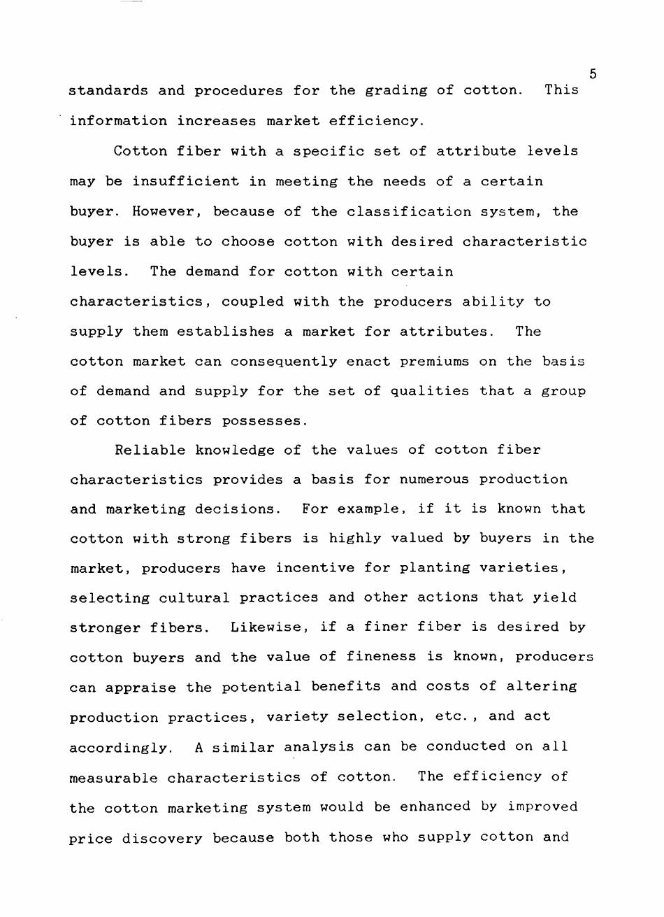
5 standards and procedures for the grading of cotton. This

information increases market efficiency.

Cotton fiber with a specific set of attribute levels

may be insufficient in meeting the needs of a certain

buyer. However, because of the classification system, the

buyer is able to choose cotton with desired characteristic

levels. The demand for cotton with certain

characteristics, coupled with the producers ability to

supply them establishes a market for attributes. The

cotton market can consequently enact premiums on the basis

of demand and supply for the set of qualities that a group

of cotton fibers possesses.

Reliable knowledge of the values of cotton fiber

characteristics provides a basis for numerous production

and marketing decisions. For example, if it is known that

cotton with strong fibers is highly valued by buyers in the

market, producers have incentive for planting varieties,

selecting cultural practices and other actions that yield

stronger fibers. Likewise, if a finer fiber is desired by

cotton buyers and the value of fineness is known, producers

can appraise the potential benefits and costs of altering

production practices, variety selection, etc., and act

accordingly. A similar analysis can be conducted on all

measurable characteristics of cotton. The efficiency of

the cotton marketing system would be enhanced by improved

price discovery because both those who supply cotton and

6 those who demand cotton are able to transmit information

that is otherwise unavailable.

While the value of price discovery knowledge is

evident, there are many obstacles which impede the price

discovery process. For instance, cotton, like all

agricultural products, is subject to price variation from

the weather, which affects its supply. Intervention into

the cotton market by nonmarket forces is also common and

provides changes whose magnitudes are often difficult to

predict.

The prime benefit of effective price discovery is

improved market efficiency through information. Farmers

often rely on the spot markets for information concerning

cotton prices. Researchers have found that discrepancies

exist between market prices and spot prices (Ethridge and

Mathews, 1983). In addition, there are no requirements for

reporting transactions and this necessarily implies

incomplete information.

Previous price discovery analyses on cotton have been

conducted (Ethridge and Davis, 1982; Hembree, Ethridge and

Neeper, 1985). These studies expressed the price of cotton

as a function of its characteristics. The approximate

value of the attributes were derived but noncharacteristic

factors were not identified.

While a perfect price discovery procedure is well

beyond existing methods and data, any analysis more

accurate than that presently in operation may provide

benefits to buyers and sellers through increased

information at lower costs. Buyers could combine the

estimated values for specific characteristics and more

accurately assess the point at which the marginal value

product of the attribute is equal to its marginal cost.

Sellers could alter production practices to produce cotton

that satisfied the desires of the cotton buyers and

therefore increase the value of the product.

Objectives

The principal objective is to estimate market values

of individual cotton fiber characteristics in the U.S.

market. The specific objectives are to:

1) Identify market variables which affect the value

of cotton and individual cotton fiber

characteristics,

2) Estimate model parameters.

3) Interpret the model for use in estimating prices

for cotton with specific characteristics.

Overview of Procedures

The selection of characteristics was made through an

examination of the attributes used by the Spot Market

Quotations and those employed in previous empirical studies

of characteristic cotton pricing. While these studies have

8 estimated characteristic market values by expressing the

price of cotton as a function of characteristics, this

study developed an alternative method which expresses price

differences as a function of characteristic differences.

This analysis estimates the variation in cotton prices

which occur due to variation in cotton characteristic

levels. An examination of the changes in the

characteristic market values over time was also conducted.

The market values of cotton fiber characteristics were

expressed as a function of the characteristics in a

particular lot of cotton, as well as exogenous demand

shifters. This analysis demonstrates the affects the

exogenous variables have on characteristic market values.

Since the price of a lot of cotton is dependent on the

actual level of cotton characteristics as well as their

market values, an examination of was undertaken to estimate

the affects that weather variables have on fiber

characteristic supplies. Regression analysis was used in

each model to estimate parameters.

In the following chapters a procedure is documented

which provides a method of estimating the market values of

characteristics and their affects on the price of cotton.

It is also shown that the level of certain characteristics

also affect the market values of other characteristics.

Finally, an examination of the weather variables that

affect the actual physical characteristic levels of the

cotton fiber is presented.

CHAPTER II

REVIEW OF LITERATURE

The central point to the characteristics approach is

that consumer preference is a preference in relation to a

collection of characteristics. When a product varies, it

is because the collection of characteristics has varied.

Given this assumption, the effects of a change in

characteristics may be evaluated. The review of literature

is organized as follows: characteristic demand theory is

reviewed nonagricultural empirical studies are reviewed,

noncotton agricultural studies are discussed, and cotton

characteristic pricing research is reviewed.

Characteristic Demand Theory

Lancaster (1971) is generally credited with the

development of the characteristic approach to consumer

economic theory, though applied studies had been conducted

prior to his analysis. Lancaster maintained that a good

was not valued for itself but for the characteristics that

the good contains. As such, each good is a collection of

characteristics for satisfying a consumer's desire for the

characteristics themselves. "The good, per se, does not

give utility to the consumer; it possesses characteristics,

and these characteristics give rise to utility" (p. 134).

10 Lancaster explained that through the characteristics

approach, theoretical problems arising through product

differentiation may be solved. He maintained that under

traditional economic theory it is not possible to verify

that wood will not be a close substitute for bread since

there is no reason except taste that they should not be.

However, under characteristic theory, they are not close

substitutes since the attributes are not similar. Also,

under traditional theory, the individual is affected by all

price changes; Lancaster stated that the individual would

not be affected by price changes that did not alter the

part of the efficiency frontier that contained his choice.

He applied his theory to such issues as the introduction of

new products, occupational choice and Gresham's Law,

explained why traditional consumer theory is unable to deal

with them, and explained how characteristic analyses could

be employed.

Lancaster concluded

In this model we have extended into consumption theory activity analysis, which has proved so penetrating in its application to production theory. The crucial assumption in making this application has been the assumption that goods possess, or give rise to, multiple characteristics in fixed proportions and that it is these characteristics, not the goods themselves, on which the consumer's preferences are exercised. The result, as this brief survey of the possibilities has shown, is a model very many times richer in heuristic explanatory and predictive power than the conventional model of consumer behavior... (pp. 154-155)

11

Rosen (1974) postulated that product prices could be

expressed as a function of the demand and supply of a set

of characteristics that were inherent in the product

itself. Products were treated as bundles of attributes

with each attribute having a price that could be identified

through an examination of the market. Each characteristic

therefore had an implicit price and each good a vector of

implicit prices. Here, as elsewhere, price differences

generally are equalizing only on the margin and not on the average. Hence estimated hedonic price characteristics functions typically identify neither demand nor supply. In fact, those observations are described by a joint envelope function and cannot by themselves identify the structure of consumer preferences and producer technologies that generate them, (p. 54)

With Rosen's method, hedonic prices were found by

regressing the price of the commodity on all attributes

inherent to it. A set of implicit marginal prices were

then found by differentiating the price of the good with

respect to the quantity of the characteristic traded in the

market. The estimated marginal prices were then used as

endogenous variables in the second-stage simultaneous

equation models containing vectors of characteristics and

shift variables. While neither supply nor demand equations

could be identified, the fact that prices are determined at

the margin ensures the estimation of implicit prices for

product characteristics.

12 Ladd and Zober (1977) developed an economic model

based upon the analysis of Lancaster, but altered the

assumptions so that every characteristic did not have

nonnegative utility, consumption technology did not

necessarily have to be linear and that utility was not

independent of characteristic distribution among products.

The authors tested the first two theoretical deviations and

found that they were correct in their modifications. Other

analyses were suggested for testing the third.

Eight applications of the model were offered for

consideration in areas including a maximization of product

sales through product design, product quality measurement,

and identification and quantification of consumptive

services. The authors also believed that these models are

attractive alternatives to the psychological and that

sociological methods often applied to measure

consumer/product relationships.

Brown and H. Rosen (1982) found that the marginal

implicit prices derived solely from quantities do not

contribute original information to that provided by the

initial observations under the given theoretical framework.

When it is assumed that the prices are generated by a single hedonic price equation, the only way to identify the structural coefficients is by (possibly arbitrary) restrictions on functional form. When it is assumed that the prices are generated by several different equations, there may

13 be sufficient "in between" variation to generate meaningful structural parameters even without such constraints on functional forms, (p. 765)

However, they maintained that much of this problem may

be avoided by employing separate markets for estimation

purposes, though structural parameters must remain constant

across the separated markets. The authors also concluded

that identification problems erect considerable barriers to

the estimation of hedonic models.

Bartick (1987) maintained that unless instrument

variables are used to exogenously shift the nonlinear

budget constraints of consumers, the fact that prices and

quantities are endogenously determined would cause

identification problems. Bartick found that by using city

and time variables he could prevent the biased results

generated by standard Ordinary Least Squares procedures.

Nonagricultural Empirical Studies

Griliches (1971), applied the concept of the hedonic

or characteristics approach to the development of price

indices. As he stated, this approach

.... is based upon the empirical hypothesis which asserts that the multitude of models and varieties of a particular commodity can be comprehended in terms of a much smaller number of characteristics or basic attributes of a commodity such as size, power, trim, accessories.... In its parametric version, it asserts the existence of a reasonably well fitting relation between

14 the prices of different models and the level of their various, but not too numerous characteristics. (p. 4)

Consequently, by utilizing regression techniques to

hold quality considerations constant, pure price indices

may be developed to measure variations in relative prices.

More precisely, "implicit" prices or values may be assigned

to the characteristics of the good. In fact, Griliches

stated that many economists, employing hedonic techniques,

have attempted to develop models which measure the price of

living, or how much money is necessary in the present to

make an individual indifferent between a former budget

constraint, income, and price level and a present budget

constraint and price level. Hence the development of a

pure price index, with quality considerations held

•'constant, has been interpreted by some to be a utility

indicator.

Fisher and Shell (1968) asserted that any attempt to

develop a true cost of living index was fraught with

difficulties because of the problem of taste variation.

Given an ability to derive quality changes and pure price

indices, any examination of a consumer's tastes over time

is certain to involve changing indifference curves and will

consequently become an intertemporal comparison of

utilities even though only one person is involved. When

15 many people are involved, the problem becomes much worse.

The authors concluded that true cost of living indices were

without foundation.

Dhrymes (1967) studied the construction of price

indices corrected for quality change in the automobile and

refrigerator industries and recognized that pricing in many

sectors was a function of price policy and not necessarily

a pure function of physically identifying characteristics.

Dryhmes states that

.... unless we conclude that all manufacturers pricing functions are statistically indistinguishable and unless we can interpret the coefficients as representing consumer (market) evaluations of the quality content of the identifiable characteristics, we cannot, strictly speaking, construct Equality corrected' price indices routinely in the manner suggested by Court and Griliches. (p. 93)

Dryhmes was unable to arrive at a conclusion

supporting the hypotheses of Court and Griliches and said

that any equation estimating the relationship between price

and characteristics was not actually a market evaluation of

the characteristics, but was, if anything, a producer

evaluation of the characteristics.

Goodman (1978) examined the market for housing in the

New Haven, Connecticut Standard Metropolitan Statistical

Area (SMSA) from 1967-1969 using hedonic methods. The

author separated the market into submarkets by employing

inherent physical components and neighborhood attributes.

By holding 1 of the characteristic sets constant, he was

16 able to determine the influence of the other in explaining

the variations in prices of homes for each subraarket.

Goodman employed the Box-Cox transformation procedure

and regression analysis in each submarket. He discovered

that suburban homes were generally 10-20 percent cheaper

than central city homes with similar characteristics, but

that the rate of difference in price diminished as housing

quality increased. He stated that given the nature of the

housing market for the period, movement from the city to

the suburb was expected. Goodman also found, by separating

the market areas across space and time, that coefficients

of attributes were not constant because improvements in

structural quality were valued more highly in suburbs.

Linneman (1980) also studied the market for housing

through hedonic price theory, though the focus of his

investigation was the development of a theoretically

appropriate model. The functional form of the model was

developed through the use of Box-Cox transformations due to

the absence of theoretical foundations for form

specification in hedonic theory. The Box-Cox search was

limited to 5 independent variables and the dependent

variables due to the dichotomous nature of the remaining 25

independent variables.

Maximum likelihood estimates were developed for rental

and owner value equations in Chicago, Los Angeles, and the

nation using the thirty independent variables (neighborhood

17 traits) during 1973. The author used standardized beta

coefficients to determine the marginal implicit prices of

the neighborhood characteristics. Neighborhood attributes

were found to be more important to property owners than

renters and explained 17 to 48 percent of site valuation.

The marginal implicit prices were evaluated at the mean to

determine the effects of varying characteristic levels on

price. For example, it was shown that housing expenditures

fell by $4.94 in Chicago for each year of a building's

age. Using a 2 percent capitalization rate, property

values fell by $7.40 per year.

Witte, Sumka, and Erekson (1979) used Rosen's

theoretical framework for an hedonic analysis of housing

attributes in 4 North Carolina cities. Orthogonal rotation

was used for data reduction, then bid and offer functions

were generated using characteristic interaction variables

to determine implicit price levels. The interaction of

variables ensured nonlinearity in first stage estimation.

The authors found that the price of housing was

predominately affected by dwelling quality. The implicit

price of a unit of this variable caused the price of

housing to vary from $57 to $87 per year. Increased

dwelling space increased the price of housing from $6 to

$38 per square foot, while increased land size had much

smaller affects.

18 Milon, Gressel, and Mulkey (1984) investigated land

prices with respect to environmental characteristics.

Three sites in the Apalachicola Bay area of northwest

Florida were ;jclected as the sites. Sales and attribute

(lot size, distance from the gulf, water frontage, etc.)

data were collected for the period 1976-82. The deflated

prices of the land segments, and characteristic data were

examined through maxiraimum likelihood estimation after

employing unrestricted Box-Cox transformations to specify

the functional form of the model.

The results of the hedonic analysis showed that form

specification had a large effect on the results. For

instance, distance from the gulf reduced the value of a lot

for the first 500 hundred feet (36.2 percent average),

declined in rate (50 percent after 1000 feet), then became

insignificant. A linear version of the model overestimated

the the decline of a site value by 630.6 percent, while the

logarithmic version of the model underestimated the decline

for the same site by 26.9 percent.

Palmquist (1984) utilized the 2 stage hedonic

estimation process formulated by Rosen and the

modifications suggested by Brown and Rosen to develop an

hedonic econometric model for housing. The author modified

Rosen's approach by assuming that the consumer is a

pricetaker and thus unable to alter equilibrium prices.

19 This is somewhat different than a price

taker in the typical market for a homogeneous product because the consumer can influence the marginal price paid by varying the quantity of the characteristics purchased, but he cannot influence the overall price schedule. The problem reduces to the consumer maximizing utility subject to an exogenous nonlinear budget constraint. The supply of characteristics was important in determining the hedonic price schedule but is exogenous for a given consumer, (p. 395)

This study avoided identification problems common to

other studies and allowed the construction of

characteristic demand equation estimations. Demands for

attributes such as living space, number of bathrooms,

central air conditioning and neighborhood quality were

developed. All variables were found statistically

significant and with expected signs.

Shonkwiler and Reynolds (1986) examined land prices on

that bordered on urban areas. It was postulated that those

areas that have desirable environmental characteristics

would have higher values than those with less desirable

attributes. Land values of the Sarasota-Brandenton,

Florida, area were obtained from the Production Credit

Association and Federal Land Bank from February 1973 to

October 1981.

The price per acre of this land was regressed against

characteristic variables using Ordinary Least Squares (OLS)

and Instrumental Variable (IV) methods of estimation. The

authors found that by separating the land parcels into 2

20 segments, commercial and residential, implicit

characteristic prices could be estimated for each. They

also found that while the implict characteristic prices

were very similar for both segments, woodlands were desired

by residential buyers but not by commercial interests.

Comparison of OLS and IV estimates using residential

and commercial indicator variables showed that if land had

commercial potential it was valued 57 percent higher using

OLS and 357 percent higher using the IV technique. If land

had residential potential, value rose by 16 percent under

OLS and 95 percent using IV. In addition, the authors

found that the ability of a land parcel to sustain

agricultural production had little effect on commercial or

residential demand. Instead, the value of urban-rural

fringe area land prices were determined to be a function of

urban development potential.

Zorn, Hansen, and Schwartz (1986) used hedonic price

theory to estimate the general impacts of growth control,

the effects of this policy on lower income households, and

government attempts to reduce the effects of growth control

on housing prices in Davis, California. In this study, the

authors gathered data on new and used home sales in Davis,

Woodland, Roaeville, and Rancho Cordova, California, for

the period 1971-1979. Prices of the homes were regressed

against a set of housing characteristics with Davis as the

focus of the study and the other cities serving as control

21 communities. This procedure allowed an ex-ante and ex-post

examination of growth control and the effects of it with

regard to housing quality and price.

The authors found that growth control increased the

price of housing in Davis, vis-a-vis that of the control

groups, because of a decrease in available housing. At the

same time, government attempts to offset housing price

increases were found to be successful for lower priced

homes. These price reductions occurred because developers

were given incentives to build smaller, lower quality

homes. The authors also concluded that attempts to

mitigate price increases only shifted the price increases

to older, higher quality homes.

Kinoshita (1987) developed a model that examined

hedonic wages under the assumption that working hours are

indivisible rather than divisible goods. By viewing

working hours as indivisible goods, it was shown that labor

can be differentiated according the characteristic length

of working hours. The wage rate (i.e., hedonic price) is a

function of this attribute.

Kinoshita deduced that under an indivisibility

assumption, the elasticity of the hedonic wage curve with

respect to wages must be greater than 0 or less than

-1. He also showed that the elasticity of the wage curve

must be positively sloped if the elasticity of production

22 with respect to hours is greater than that of production

with respect to employees.

Jones (1988) used a Lancastrian characteristic model

to estimate the attribute values of vitamins contained in

consumer food items. He found that most of the vitamins

had the correct sign and were significant though the prices

tended to be overestimated by the model.

Jones also briefly examined the labor market through

wage regressions. While no statistics were supplied by the

author, he noted that the behavior of the characteristic

coefficients reacted significantly when the data is divided

along North-South lines, blue collar-white collar, etc. He

explains that the rationale for this has been attributed in

the past to labor immobility but that if this were true,

wages would be expected to increase more per unit of a

characteristic in a sample where the characteristic is more

scarce. This was not found to be true, and the author

stated that this was a puzzle. He also noted that

Lancaster assumed divisibility of characteristics whereas

Rosen assumed indivisibility. Jones found no reason to

assume that the relation of product prices to

characteristics would be significantly affected by the

assumption of characteristic divisibility.

23 Noncotton Agricultural Models

Waugh (1929) investigated the relationship between the

prices of cucumbers, tomatoes, and asparagus and their

quality characteristics. Using univariate methods of

analysis, he found that premiums were enacted for

characteristics that were more highly valued by the

participants in the market.

Ladd and Suvannunt (1976) developed the consumer goods

characteristics model (C.G.C.M.). The model was based on

the Lancastrian assumption that products are desired by

consumers because they provide utility to the consumer.

The level of utility was a function of the characteristics

that the products contained. Total utility derived by the

consumer was dependent on the quantity of the desired

characteristics purchased by the consumer. Using these

statements as premises, the authors constructed a

theoretical model, C.G.C.M., then performed empirical tests

on 31 food items. Implicit prices were derived for the

nutritional elements in the food items. This study

indicated that "If the relation of consumer's purchases to

product characteristics is known, a product can be designed

to maximize profit by determining how much of each

characteristic to put into the product" (p. 510).

Perrin (1980) investigated the impacts of utilizing a

component pricing mechanism rather than a commodity pricing

apparatus. With component pricing, the value of a

24 commodity is determined by the sum of the quantity of

specific attributes that the product contains multiplied by

the value of the attribute, rather than appraising the

value of the product itself. Perrin stated that such a

system may be especially useful for the agricultural

commodities that possess a significant degree of

heterogeneity in terms of quality. If differences in

quality may be discerned at a practical cost, the value of

this information may, through component pricing models,

yield significant social benefits.

Given a commodity that derives its value from two

components, A and B, Perrin constructed a comparison of

market equilibria under the commodity and component pricing

methods. Under commodity pricing, the implicit prices of

components are equal since neither are accounted for in the

value determination. The ratio of the 2 attribute values

is equal to 1 and the slope of the iso-revenue curve is

equal to -1. Perrin expected a different equilibrium to

occur with component pricing because of the low probability

that the implicit prices would be equal. Equilibrium would

occur where the component price ratio is equal to the

implicit producer price ratio and the marginal rate of

transformation for A and B. This will probably yield an

increased production of one of the components. If

information costs are high, an equilibrium similar to the

commodity pricing method is more likely.

25 For soybeans and milk, Perrin found that the social

benefit of component pricing would be approximately 2

percent and that even such a small figure as this may be

overstated because of the absence of information costs, and

component transformation data for the characteristics of

the commodities.

Brorsen, Grant, and Rister (1983) constructed an

hedonic estimation model to examine the qualities that were

important in the valuation of rice bid/acceptance markets.

The authors found that federal grades could not fully

explain quality differentials. Discounts were estimated

for a number of factors. These discounts enabled rice

producers to more accurately determine the value of their

commodity than when the producers placed sole reliance on

the present grading system.

Carl, Kilmer and Kenny (1983) undertook a study of

potato contract prices. An hedonic estimation procedure

was conducted that sought to discover the implicit value of

services contained within the contracts. The authors

concluded that price differentials were indeed a function

of the service inherent in the contracts.

Wilson (1984) utilized the hedonic techniques of Rosen

to study the characteristics of the malting barley market.

An econometric model was constructed which regressed barley

prices against several commodity attributes. Marginal

implicit prices were derived from the hedonic price

26 equation for characteristics. Like Brorsen et al. , Wilson

found that federal grades did not adequately explain price

variation.

Jordan, Shewfelt, Prussia, and Hurst (1985) segmented

the market for fresh tomatoes in an attempt to analyze the

variation in implicit prices caused by different handling

techniques. A sample of 1694 tomatoes from Florida,

Georgia, and North Carolina harvested during the months of

April, August, and September was examined. The attributes

and the prices of these tomatoes were recorded. A separate

hedonic equation was estimated for each month using

iterative Ordinary Least Squares on a Box-Cox transformed

model. Implicit price shifters were not identified for

supply because the brevity of the time period allowed the

assumption of fixed supply.

The authors stated that a palletized system of

handling the tomatoes caused less damage to the quality of

the produce than a handstacking system, but was more

expensive. An examination of implicit price changes due to

handling techniques and a knowlege of the costs of these

techniques led the authors to conclude that the palletized

system was economically feasible. However, they offered

the caveats that other factors (training and supervision)

were important and that additional handling techniques

should be considered.

27 Eastwood, Brooker, and Terry (1986) constructed a

model similar to that developed by Ladd and Suvannunt in

which implicit prices were derived for nutrients in food at

the household level. Demand equations were then derived

for the nutrients using imputed prices, income, home

location and size, age, education, and race across

households. Results of this study indicated that consumers

were cognizant of nutrient levels when purchasing food and

that this was reflected in the prices paid for the goods.

The authors concluded that since consumers are willing to

increase food expenditures in return for higher nutrient

amounts, advertising nutrient levels would be an effective

procedure for the promotion of foods with desirable

attributes.

Cotton Characteristic Pricing Research

Several studies conducted in the first half of

thiscentury anticipated the hedonic research of the

present. These papers focused on the relationships that

existed between premiums and discounts and the classer's

determination of grade and staple. Univariate statistical

analyses were the predominant method of analysis. Hedonic

analysis on cotton was reimplemented in the 1970's. Much

of the relevant literature was reviewed by Neeper (1985)

and a synthesis of much of that work is presented here.

28 Taylor (1916) used 38,000 monthly data points

representing lot and single bale cotton sales obtained from

73 markets in 9 states to examine correlations between

average price and grade and staple on a monthly basis.

Crawford and Gabbard (1928) amassed cotton sales data on

markets in the 4 cotton producing regions of Texas from

samples obtained from local buyers and producers.

Paulson and Hembree (1934) examined data from 24 Texas

markets for the period 1926-33. Premiums and discounts

were viewed in relation to the classers determination of

grade and staple for an evaluation of the daily spot

quotations. Howell and Burgess (1936) recorded cotton

sample grade and staple classification along with buyer

type from markets across the southern tier of the United

States. These data were examined in relation to producer

prices for the samples during the period 1929-32. Howell

and Watson (1939) duplicated this study for 1933-36.

Central market prices were also contrasted with local

market prices. Howell wished to include assessments of

"character" in his studies but was prevented from doing so

because of the absence of a classification procedure. He

concluded that local and central market prices possessed

different premiums and discounts. Local markets were found

to have their own levels of price variation and the degree

of price variation was a function of the average cotton

quality for the market area.

29 Newton, Burley, and Laferney (1965) evaluated the

correlation between producer prices established through

classification discounts and premiums and the use value of

cotton lint. A random sample of 48 bales and their market

prices were obtained from California, Mississippi, and

North Carolina. They found that discounts and premiums

enacted on classification of grade, staple and micronaire

did not accurately correlate with the use value of the

cotton. Hudson and Williams (1975) examined the Louisiana

market. Their objective was also an examination of price

and use value correlation. Models using 1965 price and

spinning test data employed multiple regression techniques

to examine correlations between spot premiums for grade,

staple, micronaire, length uniformity, 2.5 percent span

length, and strength and use value. They found that price

differentials were not accurately explained by mill

efficiency value.

Horak (1976) used USDA data from 1964-75 to formulate

a model to predict cotton prices through an examination of

fiber properties. Step-wise regression techniques were

employed to select variables and to estimate the efficiency

of various models. One model was constructed solely of

fiber properties. Another employed supply/demand variables

such as consumption, stocks, and production. A third

combined elements of the first two models. The model using

supply/demand variables was found to more sufficiently

30 explain price variation than the model dependent on fiber

properties alone. However, the most accurate model was

that which utilized fiber properties and supply/demand

variables. By separating his models into chronological

sections, Horak found that fiber properties were

increasingly powerful for explanation of price variation.

Ethridge, Shaw, and Ross (1977) used data from the

Lubbock Cotton Classing Office that were generated via high

volume instruments (HVI) for the 1976 crop. Prices were

deseasonalized from a base of January 5, 1977. These

prices were then regressed against the attributes of grade,

length, micronaire, strength, and length uniformity.

Micronaire variation, and lot size were also included. The

authors found all variables to have significant impacts

with the exceptions of strength and length uniformity. The

lack of effect from these variables was postulated as being

due to the absence of sufficient variation for the

characteristic levels. Robinson, Ethridge, Shaw and Rogers

(1979) found similar results.

Ethridge and Davis (1982) used methods initially

presented by Rosen to derive implicit prices for a numberof

attributes common to the commodity cotton. The authors

began the paper by discussing previous work on the subject

of hedonic pricing and its implications in general, then

its relation to cotton in particular.

31 The authors noted fiber length, micronaire, color, and

trash content characteristics (and their determination),

then regressed these characteristics against the price of

cotton for the years 1976-77 and 1977-78 using the

Generalized Least Squares (GLS) technique. While all

coefficients were found to be statistically significant for

both years, their respective contributions toward the

explanation of cotton prices was variable. The point was

made that the supply of the various characteristics may

have changed between periods due to weather or a number of

other factors.

The study concluded that by observing that while many

other factors may influence the price of cotton, the

characteristics of the commodity itself have a substantial

impact. Producers might utilize the information for

variety selection, while policymakers might employ it in

recommendations for genetic research or educational

programs. Ethridge, Sudderth, and Moore (1983) constructed

a model to predict values of cotton varieties. Since

characteristics are a function of varieties, and because

price is a function of characteristics, the value of cotton

to producers is dependent on the yield and the

characteristic values.that are genetically inherent in

varieties. By estimating prices and yields for given

varieties, the authors were able to establish a monetary

value for a specific variety.

32 Ethridge and Mathews (1983) evaluated the efficiency

of market information produced by the Daily Spot Cotton

Quotations (DSCQ) Committee for the West Texas Cotton

Market. The authors examined price discrepancies that

resulted from a comparison of the discounts and premiums

reported from the Telcot marketing system and those

reported by the DSCQ for 1980-81 and 1980-82 marketing

years. Telcot and DSCQ prices varied by as much as $. 15

per pound.

Prices for base quality cotton (grade 41, staple 34,

3.5-4.9 micronaire) were similar, but discounts varied in

response to staple, 1980-81 micronaire groups, and the

upper range for trash levels. The results have

implications for futures markets in cotton.

In contrast to the Dryhmes model, Hembree, Ethridge,

and Neeper (1985) examined a market where producer input

into price determination is minimal. This study viewed the

effects of cotton fiber properties on U.S. landed prices at

textle mills. Using attribute information provided by HVI

determinations, the authors sought to discover marketplace

assignation of value for the characteristics length, length

uniformity, strength, micronaire, whiteness, yellowness,

and trash content. Landed mill prices were found to be

significantly affected by all characteristics listed above,

though the sign of the length uniformity coefficient was

not as expected.

33 This study also found that when market conditions were

not allowed to fluctuate, fiber properties explained 85

percent of the variation in landed mill prices. This would

provide empirical support that pure price indices may be

constructed. At the same time, when market forces were

allowed to vary, the characteristics of cotton explained

only 17.8 percent of the price variation.

Jones-Russell, Sporleder, and Talpaz (1986) used

Lancastrian characteristic analysis to derive implicit

prices for yarn counts and spinning techniques. The

authors estimated the shadow prices of fiber

characteristics for various yarn counts and discovered that

these values vary significantly as yarn counts are allowed

to fluctuate. Marginal implicit prices were obtained and

were found to vary with the spinning technique employed.

Bowman and Ethridge (1987) reformulated the Hembree

et al. econometric model to investigate the relationship

between U.S. mill prices of cotton and its inherent fiber

characteristics using data from 1977-1986. The authors

found that, while holding other characteristics constant,

if the length of a sample increased by one tenth of an

inch, the value of the cotton increased by 2. 1 cents per

pound, and as strength increased by one gram/tex, mills

paid an added 1.3 cents per pound. Likewise, an increase

in the trash code of 1 unit caused the value of the cotton

34 to fall by 2.5 cents per pound. Fiber characteristic price

flexibilities were also derived.

Ethridge and Neeper (1987) estimated implicit prices

for cotton fiber characteristics in Texas and Oklahoma for

the 1983/84 and 1984/85 marketing years. The focus of the

study pertained to the fiber qualities of strength and

length uniformity. Neither attribute is currently included

as a basis for spot market premiums or discounts though 90

percent of the study crop was evaluated for the

characteristics.

The authors employed a multi-equation model and

seemingly unrelated regression (SUR) to estimate the

significance of the relationship between fiber strength and

length uniformity and concluded that these measures should

become universally reported because market participants had

already begun to respond to them as valuable information.

The authors noted that increased information regarding

sample attributes would enhance the operational efficiency

of the cotton fiber market.

Jones-Russell and Sporleder (1988) estimated the mill

end-use demand for cotton fiber. The authors found that

that prices, yarn prices, and the type of spinning

technology employed significantly affected the the demand

for cotton. Jones-Russell and Spoleder employed Seemingly

Unrelated Regression techniques and found that end-use

demand for cotton in cotton/polyester fabric blends was

35 more greatly affected by changes in the price of polyester

than by changes in cotton prices. The authors also found

that the prices of polyester and cotton were complements

rather than substitutes.

CHAPTER III

CONCEPTUAL FRAMEWORK

In this chapter, the conceptual basis of hedonic price

theory is presented. Because this theory is of relatively

recent origin, and is still evolving, terms are defined and

examples are presented to aid in the clarification of

important points. The chapter is organized in 2 sections.

The first deals with the general hedonic concept as applied

to products in general and to cotton in particular. The

second part presents some conceptual modifications with

applications to cotton pricing.

The Hedonic Pricing Concept

Fundamental to hedonic price theory is the assertion

that the demand for any good is a derived demand for the

characteristics inherent to the good itself. It is the set

of identifiable characteristics that a consumer desires

rather than the good. For example, under hedonic theory,

consumers purchase automobiles because of sets of

characteristics. The sets of characteristics might include

a specific engine, 4 wheels, a particular interior

upholstery, a type of transmission, etc. This purchase is

for an automobile is because the good demanded has

characteristics attributed to the product automobile.

36

37 The conceptualization of the hedonic approach to

commodity analysis requires that a product be viewed as a

bundle of characteristics rather than as a homogenous

product. Characteristics (attributes) are homogeneous in

composition while a good is heterogeneous inasmuch as it is

composed of a differentiable set of homogeneous

attributes. Since each characteristic possesses value to

the consumer and the consumer purchases the good because of

the characteristics inherent to it, the value of the good

can be expressed as a sum of the values of the pertinent

characteristics. A characteristic value is a

multiplicative combination of the number of characteristic

units in the sample and the "implicit" price of a unit of

that characteristic. In other words, the characteristic

value is the price of the characteristic multiplied by the

level of the characteristic. If the implicit price is

positive, an increase in the amount of the characteristic

will increase the value of the product. If the implicit

price is negative, an increase in the amount of the

characteristic will cause a decrease in the value of the

product. The hedonic function is the disaggregator which

allows the implicit prices of each characteristic to be

"discovered.

An example may clarify the hedonic concept. If

supermarkets stocked grocery carts with varied assortments

of items rather than placing the items separately on

38 shelves and consumers were free to choose any market basket

from a set of market baskets, each consumer would select

that basket which yielded the highest level of utility

given his particular set of preferences (Triplett).

While the prices of the baskets would be in reference

to the baskets themselves, consumers would base their

choices on the items which are contained within the

baskets. Consequently, the price of a single item would

not be directly observable. Hedonic theory disaggregates

the prices of the goods within a particular basket to

discover the price of single items, or the "implicit"

prices. This is possible because all transactions occur at

the equilibrium price established for each given basket.

At this equilibrium, the quantity of a good implicitly

demanded through the purchases of market baskets is equal

to the quantity of the good supplied. Given equilibrium,

the price is a function of the implicit price of the goods

contained in the basket. Consequently, the price for each

good is established indirectly via market forces even

though no good is offered separately.

In fact, it is only through shared characteristics that

goods may be called substitutes. Trucks and automobiles

are discernable substitutes. This is because they share

characteristics; an engine, 4 wheels, a transmission, etc.

They are different because each has attributes not common

to the other. Motorcycles are also substitutes for

39 automobiles, albeit much weaker, because they have fewer

shared characteristics. It is only through shared

characteristics that goods may be substitutes. This is not

possible under the limitations of traditional economic

theory (Lancaster) in which substitution must be derived

from empirical analyses.

On the supply side, when a car manufacturer produces

automobiles, he is producing sets of characteristics which

are subsets of the attributes referred to as automobiles.

Since consumers of automobiles are not homogeneous, the

manufacturer varies the sets of characteristics. While

each set of characteristics is an automobile, the variation

of attributes and their monetary values will yield numerous

product prices.

The concept of value in hedonic theory is also unique.

A good has value to the extent that the characteristics

inherent to the good have value. Characteristic value is

determined by multiplying the amount of the attribute

contained in the good by the "implicit" price of a unit of

the characteristic. The value of the good is a summation

of the values of all characteristics contained in the set

of characteristics that define or comprise the good. No

good has value in and of itself, only through the value of

its characteristics. In the case of automobiles, each

characteristic adds (or subtracts) an amount to the total

value of the automobile. Also changes in the value of a

40 good arise from variations in the values of the

characteristics. For example, during the 1970's oil prices

rose quickly in the United States and the demand for

automobiles changed. Consumers wanted smaller cars with

more fuel efficient engines.

Characteristic quantity also influences implicit price

variation. If a large number of cars were produced but

only one hundred convertibles were produced in a market

period, the prices of most cars would fall because of the

decline in value of the sum of their attributes. Those

automobiles which had the characteristic of a convertible

top in their attribute set would not experience the same

decline in overall value because of the increase in the

value of the convertibility attribute.

Given the assumption that characteristic demand curves

are downward sloping, and that characteristic marginal cost

curves are positively sloped, the equilibrium implicit

price for each characteristic will be revealed at the

intersection of these curves, i.e., the characteristic

market equilibrium. While this process does occur in goods

which are heterogenous (differentiated), it is not directly

apparent because the characteristics are not overtly bought

and sold in the market place.

41 Hedonic Pricing Applied to Cotton

There are approximately 90,000 producers of cotton in

the United States and a multiple of this number worldwide.

Consequently, the domestic producer is usually viewed as a

price taker facing a perfectly elastic demand curve. Under

this assumed market structure, the producer, regardless of

his actions, cannot influence the price determined for his

commodity. If the producer attempts to establish a price

for his cotton above the established value, he will receive

no revenue because buyers are able to obtain all the cotton

they desire at the lower market price. If the producer

assigns a price below the equilibrium price, he will sell

all of his product, but at a profit that is less than he

could have earned by selling at the market price.

However, perfect competition may not be the most

accurate market structure applicable to cotton when quality

is considered. In the assumed market structure above,

cotton is traded as a homogeneous good because the

perfectly competitive model demands this assumption.

Cotton, traded in bales and mixed lots of bales, is in fact

a heterogeneous good and is viewed as such by the

participants of the market. Before cotton is offered to

the market, each bale.is classed with respect to its color,

contaminant content, length of fiber, and micronaire

reading; in some cases fiber strength and length uniformity

is also determined. Given the set of currently measured

42 attributes, and the range of variation for each attribute,

several thousand commodity classification attribute sets

exist.

Monopolistic competition is proposed as an appropriate

market structure for an examination of cotton when quality

is considered. Under monopolistic competition, it is

necessary to have a market with a large number of sellers

supplying a differentiated product. Cotton has a large

number of sellers and is a differentiated product because

it may be composed of a set of characteristics that have a

wide distribution of measured levels. Thus, the

differentiated product has a negatively sloped demand

curve, though demand may be highly elastic. Producers may

be able to influence the price they receive to some extent

by supplying cottons that possess the characteristics most

highly valued by the market. Consequently, the price of

cotton becomes a function of the market values for the

various characteristics of the commodity, although the

market for each separate characteristic may be perfectly

competitive.

Following hedonic price theory, the market value of a

particular lot of cotton is determined by a summation of

the market values of the product characteristics. A lot

with highly valued characteristics will bring a price that

43 is higher than the price received by a lot with a set of

characteristics that is regarded as less valuable by the

market.

A lot, S, has an amount of characteristic 1 equal to a,

and an amount of characteristic 2 equal to b. Assume the

hedonic disaggregator has found the implicit prices of the

characteristic 1 and 2 to be y and z, respectively. The

value of S is:

S - y*a + z*b. (3.1)

For example, the cotton attribute of fiber length is a

desirable characteristic since longer fibers produce

stronger yarns due to an increased fiber contact area

during the manufacturing process. Therefore, other things

equal, the greater the length level of a cotton lot, the

higher the lot value. To illustrate, assume a lot of

cotton of grade (GR) 42, length (L) 33 32nds of an inch and

that these are the only relevant characteristics of

cotton. The implicit prices of grade and length are y and

z, respectively, and the unit value of the lot is S, where

S = y*42 + z*33. If another lot has the same grade as S

and a length level of 34, the new value would be T, where T

= y*42 + z*34 and T > S. Using similar analyses,

derivation for cotton.lot values is feasible for all sets

of cotton attributes. Once the implicit prices of the

relevant characteristics are known, they may be multiplied

44 by the characteristic levels to provide the value for the

cotton lots.

The monetary values for cotton lots with specific

attribute levels are not constant, but vary with the forces

of supply and demand. Characteristic implicit prices are

also equilibrium prices derived from and subject to market

determination; they should be expected to vary. Even if

the characteristic levels of a lots are held constant over

time, shifts in characteristic supply and demand would

cause characteristic values to change through effects on

implicit prices. Consequently separation of characteristic

supply and demand is necessary to explain the variation in

characteristic values due to changes in implicit price

levels. Otherwise, variation over time of implicit price

levels is not revealed.

These concepts can be restated in mathematical

notation. There is inherent to each unit of cotton a

vector of characteristics Zl...Zn (using Rosen's

symbolism). The price assigned to each lot is a function

of the level of these characteristics. Consequently,

P(Z)=P(Z1...Zn). If the price of cotton, P(Z), is

differentiated with respect to its ith factor, Zi, the

market equilibrium price function for Zi, Pi(Z), may be

specified. This is implicitly contained within P(Z).

The cotton consumer's assigned marginal price for Zi is

a function Fi(Z,Yl) of all amounts of characteristics in

the lot in addition to a vector of exogenous variables,

45 Yl. This is because the variables are jointly dependent in

production and consumption. Attribute packages cannot be

subdivided. Yl is a vector of exogenous variables that

shift demand for the attributes.

The marginal value of Zi that cotton producers

determine is written as Gi(Z,Y2), where Y2 is a vector of

supply shifters. Pi(Z) will be the market generated

implicit price for the attribute Zi.

Products are particular types of products because they

contain particular groups of characteristics. Cars and

trucks are substitutes to a large degree because they share

many characteristics. Both have engines, wheels, and are

used for transportation purposes. However, they are not

the same product because they also possess characteristics

which are not the same. A truck has a greater capacity for

transporting goods. Cars do not have this characteristic.

Because a truck has a bed, its price will be affected.

The fact that a good contains a particular

characteristic at a particular level will affect the values

of other characterisitics. In the case of trucks, a large

bed for hauling objects is valuable only if the engine will

permit the capacity of the truck to be utilized. In this

case, the engine size.would be expected to have an impact

on the implicit discount of the truck bed. The premium for

increased capacity for the truck would be positively

affected by increases in the engine size. Additionally,

46 Rosen and other hedonic theorists have asserted that

products are composed of characteristic bundles and that

these bundles may not be "untied". Characteristic effects

on product prices are not completely separable.

A Modified Conceptualization

Lancaster maintained that goods are related only

through shared characteristics. Shared characteristics

means that goods are similar to buyers. The reason that

price differences occur can be explained by examining the

various levels of attributes that each good possesses. If

product A has 10 units of a desired attribute and product B

has 11 units of that characteristic then product B is

expected to have a higher value, ceteris paribus.

Rosen provided a an analytical framework that revealed

the implicit price of an additional unit of a

characteristic at a point in time for a specified period of

time. Later studies on cotton (Ethridge, Neeper, and

Hembree) indicated that fluctuations in noncharacteristic

factors, i.e., general supply and demand shifters, can

cause such large variation in the general price that

characteristics can only explain a minor amount of the

total variation of the price over time. Other studies

(Horak) found that as the period of time increased, the

level of explanation by characteristics diminished.

47 Consequently, an alternative method may be postulated

that allows the general price of a good to vary, yet

explains the variation in the prices due to

characteristics. This may be accomplished with the

definition of a standard, or base set of characteristics;

the price of a product with the base set of characteristics

would fluctuate according to changes in general supply and

demand shifters. The prices of goods that contain sets of

characteristics that differed in amounts from the base set

of attributes would be explained by discounts and

premiums. The market assessment of discounts is dependent

on the degree to which various characteristics differ from

the levels of the base set.

The premise for this theoretical addition rests upon

the assumption that general market prices for a good are

affected by supply and demand factors which cannot be

captured by specific characteristics. This assertion rests

on empirical studies which were conducted over time, and

which therefore allowed supply and demand factors to

change. The characteristic implicit prices found through

hedonic analyses are regression parameters. As the price

of a product changes because of the effects of supply and

demand changes, the parameters must vary, ceteris paribus.

If these parameters are not allowed to fluctuate, the

1 ^ 48

explanatory power of the characteristics will diminish.

This is due to the fact that the parameters are implicit

prices which are subject to the forces of supply and demand

(Rosen 1974).

As such, the general market price level (i.e., the

price for the base set of characteristics) is a function of

general market forces while values of specific

characteristics (premiums and discounts) are determined by

the supplies and demands for individual characteristics.

It is reasonable to assume that physical values of

characteristics embodied in a given type of product are

fairly constant, and do not vary with the same volatility

as product prices.

Because of the effects of supply and demand changes on

implicit prices, an alterative was hypothesized that would

allow general supply and demand variation to have an effect

on the general or base price of a product, but which would

not affect the parameters. This required defining the base

set of characteristics of a product as the set of

characteristics whose value would be allowed to fluctuate

according to changes in supply and demand.

Since all goods within a market are not the same, but

are instead differentiated, the degree to which the level

of characteristics of a good are different from the base

set of a product has some relation to its price differences

from the base in the market. Therefore, only the

49 characteristic deviations from the base would be allowed to

impact the respective prices of the differentiated

products.

A Model for Cotton

Assume that a base set of characteristics for a lot of

cotton consists of A units of attribute Y and B units of

attribute Z. A general or base price, BP, defines the

value of this set of characteristics. A second lot

contains C units of attribute Y and D units of

characteristic Z. Characteristic differences are defined

as the number of measurement units that a lot

characteristic deviates from the number of units of a

characteristic that are contained in the base set. In this

case, the characteristic differences would be C-A units of

characteristic Y and D-B units of characteristic Z. Given

time and location are the same for each lot, and that the

price of the second lot is SP, the value difference between

SP and BP must be attributable to differences in the level

of fiber characteristics.

A larger and more realistic example reveals a more

complex problem. Given a particular time and location, a

base set of characteristics includes E units of TR, F units

of C, G units of ST, H units of M, and I units of S. This

base set of characteristics has the base price, BP. Any

variation in characteristic unit levels from the base will

50 result in a variation of the price of a lot. If a lot

contained J units of S rather than the base level I, the

price level of the lot would vary by the characteristic

difference of J-I units of S multiplied by the market value

of a unit of S.

The aggregate discount, AD, is defined as the total

discount which occurs because of characteristic deviations

from the base set of characteristics. It may be positive

or negative in value. Characteristic implicit market

premiums and discounts are defined as the value that each

additional unit of a characteristic above or below the base

level adds or subtracts from the lot value. If a unit of

TR is valued by the market as a, a unit of C at b, a unit

of ST at c, a unit of M at d, and a unit of S at e, the

value of the aggregate discount would be:

AD=:SP-BP=a* (N-E) +b* (0-F) +c* (P-G) +d* (Q-H)

+e*(R-I). (3.2)

Characteristic implicit market discounts may then be

discovered with the use of the hedonic method as a

disaggregator (Triplett). The aggregate discount is a

function of the characteristic differences rather than the

price as a function of the characteristic levels. As a

result, the hypothesis becomes AD=f(CDi). The aggregate

discount is expresses as a function of the characteristic

differences from the base of all characteristics, l...n.

This is a corollary to hedonic price theory where P=f(Zi).

51 Using the example given above, the base set of cotton

characteristics contains a grade of 42 and a length of 34.

The base price, BP, is defined for this set of

characteristic levels. Any deviation from this set wil

receive a discount or a premium. If a lot contained a

grade of 42 and a length of 33 the discount for grade would

be zero because the lot grade is the same as the base

grade. The characteristic difference is zero.

However, for length, a discount would be assessed to

the length characteristic in the lot because it is one unit

below the level contained in the base. The characteristic

difference would be one. Consequently the price of the

sample would be the base price, i.e., the price of cotton

with grade 42, length 34, minus the market value assigned

for a unit of length. If the implicit market discount of a

unit of length was a, the price per pound of the lot, SP,

would be SP=BP-a*(l).

As has been shown, the hedonic price theory for cotton

has found price to be a function of the levels of

characteristics in the cotton. When the price of a lot of

cotton is expressed as a function of the characteristics in

the lot an implicit price is established for each

characteristic in that lot. The price per pound of the

cotton lot may then be calculated by multiplying the

implicit prices by the characteristic levels in a cotton

lot, then summing the resulting characteristic values.

52 Demand Factors

The levels of cotton fiber characteristics in a lot

affect the implicit market discounts of the

characteristics. The implicit market discount of a

characteristic can be affected by its own level in the

lot. If a lot has a low micronaire level, the implicit

discount can be affected by the degree to which the

micronaire is low; the value of additional units of

micronaire would be greater in lots with low micronaire

levels than in those with high micronaire levels. Also the

presence of a characteristic at a particular level may not

only affect the price of the lot, but may also affect the

value of each attribute in the lot.

Characteristics are expected to have the same type of

effect that they have on the price of a lot of cotton

though the magnitudes are expected to be smaller. For

example, if color has a significant impact on the

characteristic value of trash, that impact is expected to

have a negative sign.

For cotton, the technology that might influence the

implicit market discounts for characteristics has been the

change in the spinning technologies that transform cotton

fibers into yarn. Ring spinning is being replaced by open

end spinning methods and there is some evidence that the

methods do not operate most efficiently with the same type

of cotton characteristic levels (Price). This may cause

53 the premiums and discounts of particular characteristics to

be altered. For instance, if ring spinning is more

dependent on long fibers, the premium for fiber length

would decline as the open end spinning methods increase

their importance in the market.

The general level of the base price will also affect

the values of specific fiber characteristics. Higher

prices should cause the premiums of desired characteristics

to rise. The reason for this lies in the dispersion of

prices that occurs when prices rise and fall. As the price

of a good rises, the price differences between goods with

similar attributes tends to increase. Consequently,

premiums will become more positive and discounts will

become more negative.

Supply Factors

Characteristic difference variation between years and

areas arises because of variation in the quality

characteristics that are produced in each year and/or

area. A major factor which determines the level of a fiber

characteristic is the variety of cotton that is selected

for planting. The genetic properties of cotton plant

variety have a major effect on the physical attributes of

the cotton fiber. Environmental factors such as

temperature and rainfall levels also affect the development

of the cotton plant and therefore the cotton fiber

54 characteristics. Soil types, nitrogen, and other nutrient

levels, plant spacing, solar radiation, and humidity are

examples of environmental factors. Variation in the

characteristic levels cause variation in the characteristic

differences. Aggregate discounts are affected through

fluctuations in characteristic differences.

Some supply determinants affect both the general and

characteristic specific values. Rainfall and temperature

affect the general price through yield. They affect the

characteristic specific values by the effects they have on

fiber development. However, the effects of temperature and

rainfall on yield will be reflected in the general movement

of the general price. The affects on the characteristic

values will be through the changes in the characteristic

differences of the cotton fiber attributes.

No assumptions are made in regard to the expected

impacts of rainfall and temperature on fiber

characteristics. This is due to the fact that a large

number of variables are not considered in this study.

Consequently, the results derived from this

conceptualization must be considered purely empirical and

always interpreted with other things equal.

CHAPTER IV

METHODS AND PROCEDURES

In this chapter, the structural equations that are the

basis for the results are presented. The chapter begins

with a summary of the data sources, then proceeds with an

explanation of the formulation and the estimation of

hedonic price models for cotton. These model include both

hedonic price (demand) model formulation and a model based

on the hedonic discount technique. This section also

includes the characteristic supply relationships. The

third section presents the structural equations used in the

analysis, including the first and second stage equations in

the estimation. Estimation techniques are also discussed.

The last section discusses the approaches used for

evaluating and interpreting results from the model used.

Description of the Data

Sample characteristic observations were collected from

information published by the Testing Section of the Cotton

Division of the Agricultural Marketing Service (AMS), U.S.

Department of Agriculture (USDA). A total of 2967

observations were obtained from this source for the

production years 1976-1986. Each sample contained data on

the trash code (index of nonlint content), color, staple

55

56 length, micronaire index, fiber strength, and production

location.

Price information was obtained from AMS Spot Market

Quotations for the marketing years 1976-77 through 1986-87.

Each sample was priced using the spot market quotes nearest

the production location. Data were annual price and cotton

quality characteristics by region for the period 1976-

1986. Alabama, Georgia, Florida, Virginia, North and South

Carolina constitute the Southeast region. Tennessee,

Mississippi, Louisiana, Arkansas, and Missouri compose the

raid-South, while Texas and Oklahoma are th- Southwest. The

Western region contains California, Arizona, and New

Mexico.

Since climatic factors form a source of the variation

in physical cotton characteristics, monthly rainfall and

temperature data were collected for each sample during each

production year. Weather information and production

locations were correlated as closely as possible by

selecting weather stations that correspond to the area in

which the cotton sample was produced. Information on

spinning technologies was obtained from sources at the

National Cotton Council.

An examination of the regional cotton pricing markets

(Table 4.1) shows that the base prices vary between

regions. These price differences impact the values of the

cotton but not through the effects of variation in

57

T a b l e 4 . 1.

Y e a r

1976 1977 1978 1979 1980 1981 1982 1983 1984 1985 1986

A v e r a g e

P r i c e Majo r

P r i c e

6 9 . 9 0 4 9 . 6 4 6 1 . 7 0 7 0 . 9 3 7 8 . 8 7 5 7 . 7 8 6 0 . 8 4 7 0 . 6 9 5 9 . 2 4 6 5 . 12 4 9 . 4 0 6 2 . 2 8

a n d C h a r a c t e r i s t i c A v e r a g e s f o r C o t t o n T r a s h

4 . 09 3 . 9 2 3 . 9 5 4 . 3 7 4 . 3 4 4 . 07 4 . 2 1 4 . 2 8 4 . 10 4 . 3 5 4 . 08 4. 16

L R e g i o n s C o l o r

of t h e S t a p l e

S o u t h e a s t 1. 46 2 . 04 1. 07 1.29 1.66 1 .20 1.25 1. 17 1. 00 1.57 1.68 1 ^ 0

3 4 . 2 6 3 3 . 9 0 3 4 . 44 3 4 . 8 0 3 3 . 9 3 3 4 . 5 3 3 5 . 2 5 3 4 . 7 8 3 5 . 4 3 3 5 . 3 0 3 5 . 04 3 4 . 7 0

t h e F o u r U n i t e d S t a t e s M i c r o n a i r e

4 . 5 3 4 . 7 5 4 . 52 4 . 3 9 4. 5 1 4 . 8 5 4 . 2 9 4. 41 4 . 17 4. 41 4 . 6 9 4. 50

S t r e n g t h

2 3 . 02 22 . 42 2 3 . 6 3 2 2 . 9 2 2 3 . 02 2 3 . 33 2 2 . 7 1 2 3 . 2 2 2 3 . 6 0 2 3 . 2 2 2 3 . 9 5 2 3 . 19

M i d - S o u t h 1976 1977 1978 1979 1980 1981 1982 1983 1984 1985 1986

A v e r a g e

7 0 . 5 1 5 1 . 3 7 6 0 . 6 9 7 1 . 5 0 8 0 . 2 4 5 8 . 3 0 6 0 . 4 9 7 2 . 3 3 5 2 . 48 6 0 . 17 4 9 . 28 6 2 . 5 4

4 . 06 4 . 3 0 4 . 17 4 . 17 4 . 4 1 4 . 2 2 4 . 2 8 4. 13 4 . 4 5 3 . 9 1 3 . 9 6 4 . 19

1. 07 1. 15 1.07 0 . 8 8 1 .31 1. 14 1.26 1. 04 1 .71 1. 11 1.64 1.22

3 4 . 3 1 3 4 . 9 1 3 4 . 5 9 3 5 . 5 5 3 4 . 7 8 3 4 . 9 1 3 5 . 5 6 3 4 . 9 6 3 5 . 45 3 5 . 11 34 . 64 3 4 . 9 8

4. 19 4. 57 4. 58 4 . 2 0 4. 70 4 . 6 5 4. 49 4. 43 4 . 03 4. 43 4. 50 4. 43

2 3 . 2 5 2 2 . 8 5 2 2 . 7 7 2 2 . 9 0 2 3 . 13 2 3 . 24 2 3 . 05 2 3 . 6 4 2 1 . 7 7 2 3 . 9 5 2 3 . 54 2 3 . 10

58

Table 4.1. (continued) Year Price Trash Color Staple Micronaire Strength

Southwest 1976 1977 1978 1979 1980 1981 1982 1983 1984 1985 1986

A v e r a g e

1976 1977 1978 1979 1980 1981 1982 1983 1984 1985 1986

A v e r a g e

6 3 . 05 4 7 . 9 7 5 4 . 15 6 0 . 8 2 7 1 . 5 5 4 9 . 9 1 5 5 . 3 0 6 3 . 4 4 5 1 . 12 5 3 . 2 6 4 3 . 9 5 5 5 . 8 7

7 2 . 03 5 6 . 3 2 6 7 . 2 1 7 4 . 9 3 8 4 . 08 6 2 . 4 3 6 6 . 27 7 3 . 4 4 6 3 . 8 4 6 1 . 85 6 3 . 3 6 6 7 . 3 3

4 . 08 3 . 3 7 3 . 9 8 3 . 7 9 4 . 02 4 . 3 9 3 . 8 1 4 . 4 2 4 . 2 1 4 . 17 4 . 5 5 4 . 07

3 . 6 8 3 . 5 7 3 . 6 4 3 . 3 0 3 . 2 4 3 . 4 9 3 . 6 8 4 . 05 3 . 00 3 . 3 4 3 . 07 3 . 4 4

1.88 1 . 4 1 1 .50 1.45 1.82 1.87 1.74 1.98 1.59 1.80 1.95 1 .73 West 0. 92 0 . 8 9 1. 00 0 . 9 3 0 . 9 8 1. 00 0 . 9 5 1 .41 1. 00 1. 07 1. 07 1 .01

3 1 . 8 9 3 2 . 10 3 2 . 08 3 2 . 4 5 3 1 . 6 1 3 2 . 4 5 3 2 . 02 3 2 . 02 3 1 . 8 5 3 1 . 9 6 3 3 . 06 32 . 14

3 5 . 3 2 3 5 . 2 0 3 5 . 15 3 5 . 2 8 3 5 . 30 3 5 . 18 3 5 . 6 0 3 4 . 6 2 3 6 . 00 3 5 . 5 1 3 5 . 5 9 3 5 . 10

4 . 16 4 . 2 1 4 . 01 3 . 6 5 4 . 11 3 . 9 0 3 . 9 9 4 . 12 3 . 4 4 3 . 7 9 3 . 7 1 3 . 9 2

4 . 17 4 . 3 4 4 . 3 2 4 . 3 7 4. 33 4. 43 4 . 2 2 4. 10 4 . 2 8 4 . 3 9 4 . 4 4 4 . 2 8

2 1 . 2 9 2 1 . 7 5 2 2 . 14 2 2 . 00 2 1 . 7 1 2 1 . 9 5 2 2 . 07 2 1 . 9 3 2 2 . 08 2 3 . 05 2 3 . 2 2 22 . 11

2 5 . 00 2 5 . 54 2 5 . 2 8 2 4 . 7 9 2 5 . 01 2 4 . 7 2 2 5 . 2 7 2 4 . 8 1 2 6 . 6 1 2 6 . 6 7 2 6 . 8 7 2 5 . 33

59 the characteristic levels. Base characteristic levels are

constant across regions. Consequently, a regional

indicator variable should be included to take these effects

into account. Failure to include these could bias the

characteristic implicit fiber discounts.

First Stage Hedonic MoHt l

In estimating models to explain market values of

characteristics, a vector of implicit marginal values is

obtained by differentiating P(Z) with respect to its ith

argument, Zi, and evaluating it at the level of the

characteristics purchased or sold.

Pi(Z) = 6P(Z)/6Zi. (4. 1)

An initial regression of the product price, P, against the

product characteristics, estimates the marginal implicit

prices but says nothing about the underlying structure of

the characteristic markets. As for commodities, supply and

demand functions exist that constitute markets for product

characteristics. Likewise, the demand for attributes is a

function of a vector of shifters which influence the

purchasing decisions of buyers. The supply of

characteristics is a function of a vector of shifters which

influences supply decisions by producers. Since both the

supply of and the demand for characteristics are price

60 dependent, they must be estimated simultaneously. In

equilibrium,

6P(Z)/6Zi=Pi(Z)=Fi(Zl Zn,Yl) (demand) (4.2)

oP(Z)/6Zi=Pi(Z)=Gi(Zl Zn,Y2) (supply). (4.3)

Equation (4.2) states that the marginal demand of a

characteristic is a function of the amounts of

characteristics in the product (Zl....Zn) and a set of

shifters, Yl, which influence the demand for the

characteristic. This equation represents a demand function

for the characteristic i. The second equation states that

the marginal supply price of a characteristic is a function

of the amount of the characteristics in the commodity, and

a set of shifters, Y2, which influence the supply of the

attribute i. This equation represents a supply function

for the characteristic i. Because there are demand and

supply functions for each characteristic, the structural

model becomes a set of 2n equations.

The analysis of hedonic theory outlined thus far has

expressed the product price and its inherent marginal

implicit prices as short term equilibrium phenomena. When

the process is evaluated over time, the procedure is

altered slightly. For hedonic modeling over time, it is

first necessary to separate the first stage equations with

regard to time spans. This requires that each product be

regressed against its set of characteristics in each time

period. Failure to separate the equations over tin.e will

61 cause a reduction in the ability of the characteristics to

explain product prices. This is due to the fact that a

single implicit price is unlikely to describe the value of

a unit of a characteristic as the supply of and the demand

for that characteristic varies over time.

Consequently, it is necessary that first stage

estimation become a series of independent equations where

the price of the product is regressed against its vector of

characteristics for each given year.

Pt(Zt)=P(Zlt Znt) (4. 4)

where t=year.

Marginal implicit prices for each characteristic are

again evaluated at the levels of the attributes contained

in each product in each year. These marginal implicit

prices are then used as endogenous variables in the second

stage where they are expressed as functions of attribute

levels and supply and demand shifters. As with the first

stage, estimation of the demand and supply price equations

is as outlined before, except that 2nt equations, rather

than 2n, must be estimated simultaneously over the period

under study. This yields a more complete analysis since

the shifters in the demand and supply functions are

evaluated over time. .Their explanatory power is expected

to increase, other things equal, because the independent

variables fluctuate over time.

62 The evaluation of demand and supply prices over time

parallels the regression of prices against supply and

demand shifters in standard economic theory.

Characteristic demand and supply prices are defined as

functions of independent variables whose fluctuations

explain price variation. Like product prices in standard

economic theory, implicit prices represent equilibrium

conditions, and can be expressed as dependent variables in

reduced form equations (Witte et al., 1979). These

equations express marginal implicit prices as functions of

all supply and demand shift variables.

When the shift variables change in magnitude, the

implicit prices of the characteristics will vary. If the

shift variables are exogenous, knowledge of their

magnitudes and their relationships to the implicit prices

will allow an estimation of the implicit prices. Since the

price of the product is an additive combination of product

characteristic levels multiplied by their characteristic

implicit prices, prices for differentiated products may be

discovered by substituting various characteristic

combinations into the product price function.

63 A Hedonic Model for Cotton Pricing

The price of cotton, P, may be expressed as a function

of its vector of attributes, Z.

Consequently Pt(Zt)=P(Zt) (4.5)

and Pt=f(Zlt....Znt). (4.6)

For this study of cotton, Z is composed of observations for

length, length uniformity, micronaire, strength, color, and

trash content. For any lot of cotton, the market clearing

price for that sample may be expressed as a function of the

objectively measured levels of the vector of attributes.

The selection of these specific characteristics is to

a major degree reliant on the work of previous cotton

research (see Review of Literature). Research conducted in

the textile manufacturing sector also supplied information

concerning attribute selection.

The first-stage hypothesized model is:

Prt = f(STrt, Mrt, Srt, Crt, TRrt, Urt) (4.7)

where:

Prt = Price of cotton in region r, time t (cents per pound).

STrt = Fiber staple length in region r, time t (32nds of an inch).

Mrt = Micronaire in region r, time t (index).

Srt = Fiber strength in region r, time t (grams per tex).

Crt = Color in region r, time t (second digit of the grade code).

64 TRrt = Trash content in region r, time t (first

digit of the grade code).

Urt - Fiber length uniformity in region r, time t (mean/upper half mean length).

The first stage equation explains cotton prices

through the characteristics inherent to the sample. This

equation reveals the characteristic implicit prices as

measures of the effects that the characteristics have on

cotton prices.

Variable Explanations

and Parameter Expectations

Staple length and cotton price should be positively

correlated. This relationship is based on the fact that

cotton with longer fibers will produce a stronger yarn

because of increased contact area. Length also augments

the productivity of any yarn process which relies on roller

drafting in its method of production. Many textile

engineers maintain that as U.S. producers alter their

production practices to include less ring spinning that

length and length uniformity will become relatively less

important (Deussen 1984).

Micronaire is an indirect measurement of a cotton

sample's fineness and maturity. Low micronaire readings

indicate either fine fibers or fiber immaturity. Fine

fibers are desirable, but immature fibers yield yarn neps

and reduce the value of the good. Despite interpretational

65 problems with micronaire, it is an important characteristic

to textile manufacturers. An inspection of its components

and prior empirical analyses lead to the expectation of a

quadratic relationship with price.

However, an examination of the cotton pricing markets

will show that no discounts are made on cotton with

micronaire levels in the range of 3.5 to 4.9. A micronaire

level below 3.5 receives a discount and a micronaire level

above 4.9 receives a discount. In past studies a quadratic

relationship between price and micronaire was used.

However direct modeling of discounts allows the micronaire

level to be segmented into three parts, a low micronaire

level a medium micronaire level which corresponds to the

base and a high micronaire level. Segmentation also allows

direct inspection of the two discount areas and how

noncharacteristic factors may be influencing each.

Strength is expected to have a positive coefficient.

Strong fibers yield strong yarns. Some disagreements

concerning fiber strength's importance in relation to newer

spinning technologies have emerged, but cotton buyers have

never questioned strength as a desirable trait.

Color, the second component of the grade code, has not

been found to be a major factor in spinnng efficiency,

though high color levels may be indicative of lint

immaturity and nonuniformity of color may cause problems in

terms of dyeing consistency (Price 1986). However, the

66 color of cotton is often associated with the overall

quality of the cotton sample. Color is expected to yield a

negative coefficienct in relation to price.

Trash is also expected to yield a negative

coefficient. Cleaning the cotton constitutes a processing

expense and necessitates some degree of fiber damage. The

greater the amount of trash, the greater the degree of

fiber damage. It is also important to note that with

present technology it is virtually impossible to remove all

contaminants. The presence of these particles cause

imperfections in yarns and fabrics. Trash should increase

in its level of importance in relation to price. Producers

have begun to use stripper harvesting on more acreage

because of cost considerations while newer spinning

technologies demand cleaner cotton because of spinning

breakage rates.

Estimation of First Stage Hedonic Prioe Model

For each year of the study, the price of each cotton

sample was regressed against the characteristic contained

within that sample. Regional slope shifter variables were

used to allow coefficients to vary between regions. This

means that the implicit prices between regions were allowed

to vary between regions. Expected signs were obtained for

67 each characteristic and the coefficients of determination

were always equal to or above the mid 90's for each year of

the study.

The data set was then separated into the regions of

the Southeast, the mid-South, the Southwest and the West.

The first derivatives of each characteristic were

calculated to yield an implicit price for each

characteristic in each region. The implicit prices of the

characteristics for each region were regressed against the

demand shifter variables over the eleven year period of the

study using Seemingly Unrelated Regression (SUR). The

estimates obtained by SUR were generally not unique and

therefore unreliable. Many of the coefficients were also

biased because of the linear dependence of the matrices.

When demand shifter variables were deleted, signs were

obtained that were often unexpected according to previous

theoretical analysis. The model was abandoned at this time

and another was hypothesized.

A Revised First Stage Discount Model

The hedonic discount model for cotton asserts tht

fiber characteristics which differ from the set of base

characteristics will receive an aggregate discount, AD.

The aggregate discount may be positive or negative and is

again defined as the difference between the price of a

sample of cotton fibers and the price of the base set of

68 characteristics. If SP is the market price of the lot and

BP is the market price of the base, the aggregated discount

AD=SP-BP.

The characteristic difference is the measurement

difference of one characteristic in a lot from the level of

that characteristic in the base. If the level of that

characteristic C in the sample is denoted as SC, and the

level of characteristic C in the base is BC, the level of

the characteristic difference for characteristic C is CD=SC-

BC. Extending the analysis for all characteristics Ci,

CDi=:SCi-BCi.

Since the aggregate discounts for each lot is affected

by the characteristic differences ADi=f(CDi). This means

that the aggregate discount for all samples is a function

of the fiber characteristic differences of the lots of

cotton. The deviation of the characteristics from the base

levels will alter the level of the fibers' price.

Cotton has the physical characteristics of trash

(nonlint content), color, staple length (fiber length),

micronaire, and strength. For each characteristic, except

strength, a base level exists which forms the base level

for the discounts. Therefore, given an assigned base level

for fiber strength for cotton samples, the aggregate

discount for cotton samples may be presented as a function

of the characteristic differences in each lot.

n ^^ . 69

Cotton prices m the United States are reported by the

Spot Market Quotations Committee. A base price is reported

for cottons with the base set of characteristics, then

premiums and discounts are added to this base according to

the deviations of the various characteristics from the

base. This base set of characteristics is 4 units of

trash, 1 unit of color, which together constitute the grade

code. The base for staple is 34 32nds of an inch.

Micronaire has a base range. This range has a lower limit

of 3.5 and an upper limit of 4.9. Strength has no base at

present. However, since the hedonic discount technique

requires a base, strength has been assigned a base level of

20 grams per tex.

As in hedonic theory, neither supply nor demand

relationships may be identified with this procedure. This

is especially true in the hedonic discount model because a

general cotton base price is allowed to fluctuate

periodically according to supply and demand factors. If

these factors are negated through the use of discounts, a

model emerges which identifies the market clearing effects

of supply and demand relationships for all characteristic

combinations but which does not in effect, identify them.

While this model.is a theoretical departure from the

cotton hedonic models formerly conducted, it owes a great

deal to the development of price hedonic models constructed

by Horak, Ethridge and Davis, Ethridge and Mathews, and

70 Ethridge, Neeper, and Hembree. In each of these models,

the price of a sample of cotton was regressed against the

characteristics inherent to the sample using multiple

regression techniques. The coefficients expressed the

implicit prices of the characteristics. The implicit

prices explained how one unit changes in a particular

characteristic affected the price of the sample, when all

other factors were held constant.

Implicit fiber discounts as well as prices themselves

may also be subject to some regional variation. This says

that particular fiber discounts may be more severe in one

region than the fiber discount assessed in another region,

due to differences in supply and demand, regional pricing

bias, or pricing inaccuracies by the Spot Markets. Use of

slope shifting variables for the characteristics should

provide some information in regard to these regional market

implicit discount variations.

Length uniformity was initially included in the model

but was dropped from the model. In many cases the length

uniformity variable had no significant effect on cotton

price. In the years when length uniformity was

statistically significant, its presence caused fiber length

to behave erratically. When length uniformity was deleted,

staple length was highly significant and stable. As a

result, staple length was the variable that was retained.

Other studies (Hembree, Ethridge, and Neeper, 1985;

71 Ethridge and Neeper, 1987; Bowman and Ethridge, 1987) have

found length uniformity to be negatively related to price

even though textile engineers believe it increases the

processing efficiency of cotton. At present, cotton

economists have been unable to determine the reason for the

negative sign.

The basic form of the model may be illustrated as:

ADrt = f(DTRrt, CDCrt, CDSTrt, CDLMrt, CDHMrt, CDSrt, Rlt, R2t, R3t) (4.8)

where (units are the same as in equation 4.7):

ADrt = Aggregate discount for a given sample in region r, at time t.

CDTRrt = Characteristic difference for trash in region r, at time t.

CDCrt = Characteristic difference for color in region r, at time t.

CDSTrt = Characteristic difference for staple length in region r, at time t.

CDLMrt = Characteristic difference for low micronaire in region r, at time t.

CDHMrt = Characteristic difference for high micronaire in region r, at time t.

CDSrt = Characteristic difference for strength in region r, at time t.

Structural Equations

The structural equations for the model illustrate the

equations that were used in the parameter estimation

72 process. Since 11 years are included in the study and each

equation estimated for each year, the subscript t is added

to the presentation for the sake of brevity.

To separate the effects of micronaire into low, medium

(base) and high reading segments, low micronaire and high

micronaire terms were included. If a sample has a

micronaire level that falls into one of these ranges, the

other term is excluded. Since no discount is assessed if

the sample micronaire level falls into the base range, a

sample micronaire reading within this range negates the

high and low micronaire variables.

The fact that the data set may be divided according to

regions allows the use of slope shifter variables to

identify variations in implicit fiber discounts that occur

because of pricing point locations. This procedure allows

a more precise estimation of the implicit fiber discounts

under the constraints of a limited data set.

ADrt = 130 + f31CDTRt + I32CDCTRRlt + f33CDTRR2t + (34CDCTRR3t + (35CDCt + I36CDCRlt + (37CDCR2t + /38CDCR3t + (39CDSTt + OlOCDSTRlt + f311CDSTR2t + (312CDSTR3t + B13CDLMt + f314CDLMRlt + I315CDLMR2t + f316CDLMR3t + [317CDHMt + (318CDHMRlt + (319CDHMR2t + (320CDHMR3t + (321CDSt + I322CDSRlt + f323CDSR2t + (324CDSR3t + UOt (4.9)

where:

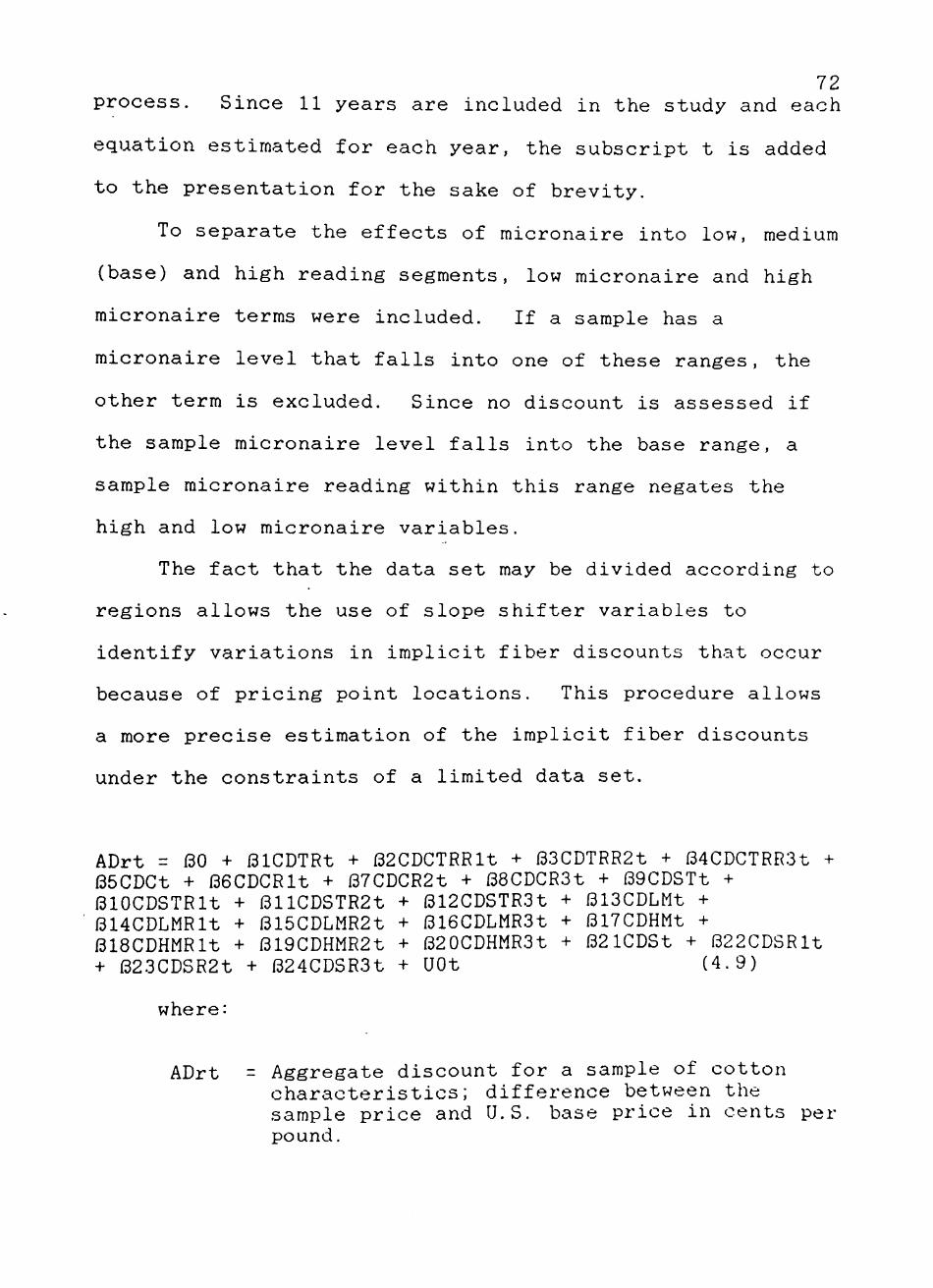
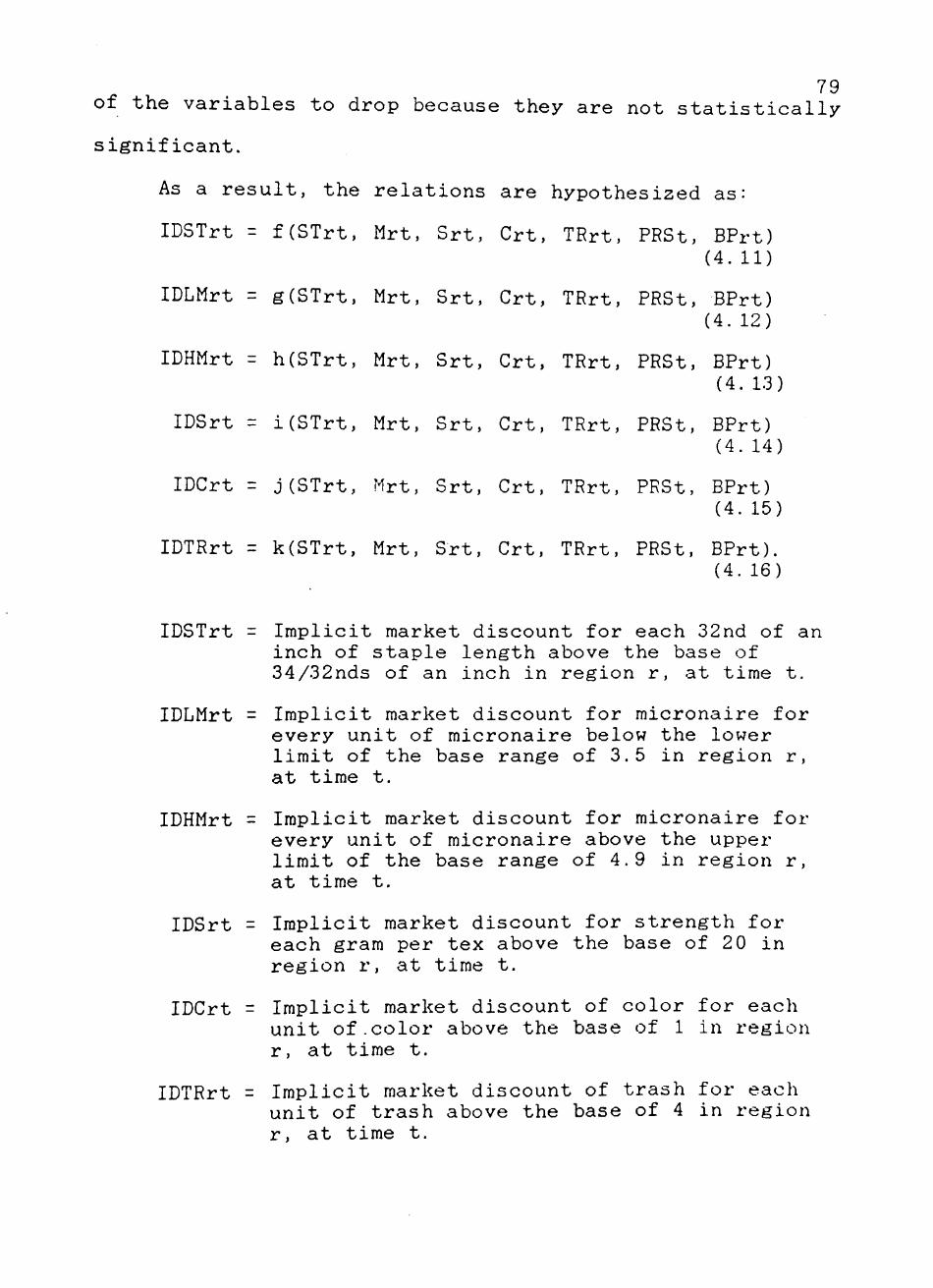
ADrt - Aggregate discount for a sample of cotton characteristics; difference between the sample price and U.S. base price in cents per pound.

73 CDTRt = Characteristic difference of trash content;

difference from the sample trash index and the base characteristic of 4.

CDCt = Characteristic difference of color; difference between sample color index and base characteristic level of 1.

CDSTt = Characteristic difference of staple; difference between sample staple length measured in 32nds of an inch and the base level of 34.

CDLMt = Characteristic difference of low micronaire; difference between the sample micronaire level and the low end of the micronaire base of 3.5 if the sample is below 3.5.

CDHMt = Characteristic difference of high micronaire; difference between the sample micronaire level and the high end of the micronaire base of 4.9 if the sample level is above 4.9.

CDSt - Characteristic difference of sample strength level and the assigned base level of 20 measured in grams per tex.

CDTRRl - Characteristic slope shifter for trash in the Southeast.

CDTRR2 = Characteristic slope shifter for trash in the mid-South.

CDTRR3 = Characteristic slope shifter for trash in the Southwest.

CDCRl = Characteristic slope shifter for color in the Southeast.

CDCR2 = Characteristic slope shifter for color in the mid-South.

CDCR3 - Characteristic slope shifter for color in the Southwest.

CDSTRl - Characteristic slope shifter for staple length in the Southeast.

CDSTR2 - Characteristic slope shifter for staple length in the mid-South.

CDSTR3 - Characteristic slope shifter for staple length in the Southwest.

CDLMRl = Characteristic slope shifter for low micronaire in the Southeast.

CDLMR2 = Characteristic slope shifter for low micronaire in the mid-South.

CDLMR3 - Characteristic slope shifter for low micronaire in the Southwest.

CDHMRl = Characteristic slope shifter for high micronaire in the Southeast.

CDHMR2 = Characteristic slope shifter for high micronaire in the mid-South.

CDHMR3 = Characteristic slope shifter for high micronaire in the Southwest.

CDSRl = Characteristic slope shifter for strength in the Southeast.

CDSR2 = Characteristic slope shifter for strength in the mid-South.

CDSR3 = Characteristic slope shifter for strength in the Southwest.

74

The i3ij 's denote structural parameters for the system,

while t and t-l denote current and past years. The

subscript r is used to denote the cotton producing region

and pricing point. UOt..U6t are the stochastic error

terms.

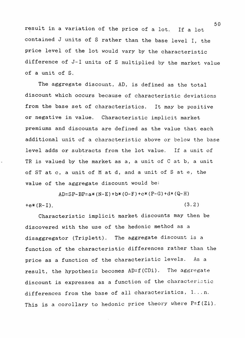
The characteristic implicit market discounts are the

first derivatives of the aggregate discounts with respect

to the characteristic differences. When the implicit

market discounts of the characteristics have been derived,

75 they may be inserted into the initial regression equation

with the characteristic differences of a specific lot to

calculate the cotton lot aggregate discount.

ADrt=IDSTrt(CDST) + IDLMrt(CDLM) + IDHMrt(CDHM) +

IDSrt(CDS) + IDCrt(CDC) +IDTRrt(CDTR) + ISRlt + ISR2t +

ISR3t. (4. 10)

The aggregate discount is then added to the base price

to determine the cotton price for the lot with the given

set of fiber characteristic levels. The price of a lot

with any combination of characteristics may be determined

by calculating the corresponding set of fiber

characteristic differences and repeating the process

outlined above.

where:

IDST = Implicit market discount for each 32nd of an inch of staple length above the base of 34/32nds of an inch.

IDLM = Implicit market discount for micronaire for every unit of micronaire below the lower limit of the base range of 3.5.

IDHM - Implicit market discount for micronaire for every unit of micronaire above the upper limit of the base range of 4.9.

IDS = Implicit market discount for strength for each gram per tex above the base of 20 grams per tex.

IDC - Implicit market discount of color for each unit of color above the base of 1.

IDTR = Implicit market discount of trash for each unit of trash above the base of 4.

76 Rl - Intercept shifter for cotton prices in the

Southeastern region. R2 = Intercept shifter for cotton prices in the

mid-South region. R3= Intercept shifter for cotton prices in the

Southwestern region.

Characteristic Demand (Second Stage) Rquationc

Characteristic demand price equations express the

implicit market discount as a function of the

characteristics inherent to the lot as well as shift

variables that may also alter the level of the implicit

market discount for the characteristic.

As stated in chapter III, the theoretical basis for

these equations is that all products are composed of

bundles of characteristics, and that the bundles of the

characteristics which compose the product may not be

untied. Characteristics are not completely separable from

each other and the presence of particular levels of one

characteristic may affect the value of another

characteristic.

For instance, the implicit market discount of trash

might be 3 cents per pound. However, this trash discount

may also be a function of the color levels that were

associated with the trash levels in the sample. This would

mean that increased levels of color might cause the the

trash discount to increase because buyers are influenced by

77 the higher color levels. This may be especially true in

the case of trash and color since together they constitute

the components of the grade code.

Likewise, implicit market discounts are expected to be

a function of their own characteristic levels. Cotton

samples receiving a discount for low micronaire are

expected to value an additional unit of micronaire while

high micronaire discounts are expected to respond

negatively to additional micronaire since high micronaire

is penalized for the number of units over the upper limit

of the base.

The characteristic values may also be affected by

noncharacteristic demand shifters. A decrease in the

proportion of domestic mills using ring spinning technology

is expected to increase the demand for strength and to

decrease the demand for length because the newer

technologies react differently to the characteristics

(Duessen 1984). Trash should be negatively related (i.e.,

discounts become increasingly negative) to the increases in

open end spinning because newer technologies are more

sensitive to trash than ring spinnning methods.

Low micronaire cottons are more acceptable to the open

end methods while high micronaire levels are less

acceptable. The changes in the discounts as technology

changes are implemented should reflect this.

78 The level of the base price should also have an

effect. The rationale for this variable lies in the

effects that the dispersion of prices have on attribute

values. As the price of a commodity rises, the spreads

between the characteristic discounts should become

greater. Likewise, when the base price falls, the spreads

between the discounts should contract. An appropriate

analogy is the behavior of air molecules in a balloon when

the temperature of air rises. Here temperature is the

proxy for price. As the heat increases, the distance

between the molecules in the ballon increases. As the heat

decreases, the distance between the molecules decreases.

An economic example may be found in automobiles. As the

prices of all cars increase, the distance in terms of price

between each car increases.

Since the objective is to see the various effects that

these variables have on the implicit market discounts in

each of the regions, the data set was separated to allow 4

models. It should be noted that the data source is

composed of quotations rather than market determined

prices. The quotations are estimates. In addition, an

examination of the quotations will show that they do not

vary consistently as the level of a characteristic varies.

In each equation, the initial hypothetical

relationship is the same, though estimation may cause some

79 of the variables to drop because they are not statistically

significant.

As a result, the relations are hypothesized as:

IDSTrt = f(STrt, Mrt, Srt, Crt, TRrt, PRSt, BPrt) (4.11)

IDLMrt = g(STrt, Mrt, Srt, Crt, TRrt, PRSt, BPrt) (4.12)

IDHMrt = h(STrt, Mrt, Srt, Crt, TRrt, PRSt, BPrt) (4.13)

IDSrt = KSTrt, Mrt, Srt, Crt, TRrt, PRSt, BPrt) (4.14)

IDCrt = j(STrt, Hrt, Srt, Crt, TRrt, PRSt, BPrt) (4.15)

IDTRrt = k(STrt, Mrt, Srt, Crt, TRrt, PRSt, BPrt). (4. 16)

IDSTrt = Implicit market discount for each 32nd of an inch of staple length above the base of 34/32nds of an inch in region r, at time t.

IDLMrt = Implicit market discount for micronaire for every unit of micronaire below the lower limit of the base range of 3.5 in region r, at time t.

IDHMrt = Implicit market discount for micronaire for every unit of micronaire above the upper limit of the base range of 4.9 in region r, at time t.

IDSrt = Implicit market discount for strength for each gram per tex above the base of 20 in region r, at time t.

IDCrt = Implicit market discount of color for each unit of.color above the base of 1 in region r, at time t.

IDTRrt = Implicit market discount of trash for each unit of trash above the base of 4 in region r, at time t.

80 STrt - Length of fiber measured in 32nds of an inch

in region r, time t.

Mrt = Micronaire reading of fibers measured in units of the micronaire index in region r, at time t.

Srt = Strength of the fibers measured in grams per tex in region r, at time t.

Crt = Color of the fibers; second digit of the grade code in region r, at time t.

TRrt = Trash code of the fibers; first digit of the grade code in region r, at time t.

PRSt = Proportion of the U.S. textile mills employing roller spinning technologies, using 1976 as the base year in year t.

BPrt = Regional base price in cents per pound in region r, at time t.

Structural Equations for Characteristic Specific Demand

The presence of other characteristics impact the

implicit discount of a specific attribute because the

characteristics are jointly purchased when the cotton fiber

is sold. It is not possible for a buyer to purchase a

certain level of a characteristic that is contained within

a lot and add it to another lot. The physical composition

of the fiber indicates that the characteristics are jointly

produced and must be jointly purchased by the buyer. For

this reason it is assumed that the levels of each

characteristic will not only have an effect on its own

implicit discount level, but on the implicit discounts of

other fiber characteristics.

81 The change in spinning methods are included in the

characteristic demand equations because the values of the

fiber characteristics are expected to be a function of the

introduction of the new open end processing technology.

While the reasons for the inclusion of this variable were

stated earlier in this chapter, it should be noted that

this variable might also have an effect on the general

price of cotton. The general price may be affected because

of the difference in processing efficiency between ring and

open end spinning methods. However, this effect would not

negate the impacts of the variable in determining the

discount values for specific characteristics. It is likely

that both affects have occurred in the market.

Following is a list of the demand equations. In these

equations, each implicit market discount is expressed as a

function of demand specific shift variables and other

characteristics. A number of shifters may not be

significant for all variables. The equations are expressed

without intercepts. Intercepts were included as an

empirical test of the propositions, but significance levels

of the variables were greatly improved when intercepts were

deleted. Signs were also more stable in the nonintercept

versions of the model.

A consequence of using the hedonic discount technique

is that the statistical methods that are applicable are

82 reduced. This reduction comes as a consequence of the

large number of zero values on both sides of all

equations. Zeroes eliminate the option of techniques that

rely upon logarithmic transformations such as the Box-Cox

method. Zarembka stated that demand theory yields little

information regarding the selection of the appropriate

functional form. As a result, functional form selection is

reduced to an iterative search process. Fuctional form

selection under these conditions becomes a matter of

circumstance. Given the method of price determination in

the United States, data at present does not exhibit stable

trends over time. This means that price quotations are

estimated by technicians with less than perfect

information. The estimates of characteristic values do not

follow consistent patterns as characteristic levels vary.

Increases in the amount of data on cotton sales should give

future researchers more opportunity to discover functional

forms with greater accuracy.

IDSTrt = iBlOSTrt + OllMrt + l312Srt+ I313Crt + (314TRrt + l315PRSrt + l316BPrt + Ulrt (4.17)

IDLMrt - l320STrt + (321Mrt + (322Srt + (323Crt + f324TRrt + f325PRSrt + (326BPrt + U2rt (4.18)

IDHMrt = (330STrt + (331Mrt + a32Srt + (333Crt + f334TRrt + f335PRSrt + {336BPrt +U3rt (4. 19)

IDSrt = (340STrt + 1341Mrt + l342Srt + (343Crt + (344TRrt + f345PRSrt + f346BPrt + U4rt (4.20)

IDCrt = I350STrt + f351Mrt + 652Srt + (353Crt + 354TRrt + /355PRSrt + f356BPrt + U5rt (4.21)

83 IDTRrt - (357STrt + f358Mrt + f359Srt + f360Crt + 136 ITRrt + I362PRSrt + (363BPrt + U6rt (4 22)

The (3ij 's denote structural parameters for the system

while t and t-l denote current and past years. r is used

to denote the cotton producing region. Ulrt...U6rt are the

stochastic error terms.

Characteristic SUPPIV (Second Stage) Equations

Aggregate discounts may be affected through two

factors: the characteristic implicit market discounts and

the level of the characteristic difference. A method for

estimating the latter has been presented in the previous

sections of this chapter. Each characteristic level is a

function of many factors and a complete analysis is beyond

the scope of this paper. In fact, this subject is only

presently being researched by cotton physiologists.

However, an attempt was made here to identify some of the

variability of cotton quality characteristics in each of

the four cotton producing regions of the United States.

As was shown in Tables 4.1 and 4.2, variation in the

fiber properties witin regions are relatively small.

However, because there are fluctuations in the

characteristic levels from year to year, an attempt was

made to identify some of the factors which affect the

levels of the fiber characteristics.

84 As stated in the previous chapter, the principal

determinant of the levels of fiber characterstics is the

variety that is selected for planting. The genetic fiber

properties inherent to the variety are those that are

apparent when the cotton is classed. The adage that what

goes into the ground is what comes out of the ground is

appropriate in this instance.

Given the complexities that arise from plant variety,

changes in plant variety, production method variations and

catastrophic occurences such as hail storms, a procedure

was selected that attempted to minmize the impacts that

these factors have on an examination of rainfall and

temperature. Variety was not included in the model because

of the lack of available data. In addition, the number of

varieties that are planted in the U.S. would require a very

large amount of data to yield statistically significant

results. In this study, variety was accounted for by

assuming that varieties within regions are relatively

stable so that their effects are captured in the separate

regional supply relationships.

Averages for each fiber property were calculated for

each region. These regional annual fiber characteristic

average were then expressed as functions of weather

variables. Weather data were assembled that corresponded

as closely as possible to each production area. The data

85 were then aggregated into the 4 regions. Weather data were

separated into seasonal periods. Monthly weather variables

were found to yield highly unstable systems and yearly

aggregations did not provide results that would explain

fiber characteristic variation over the period of the

growing season. This suggested that temperature and

rainfall data be separated into the spring, summer, and

fall seasons. Rainfall for the previous winter months and

the previous year were included in the model to test if

they too might have some effect on fiber characteristics as

well as plant development.

Consequently the average characteristic level for a

particular year is expressed as a function of the rainfall

and temperature variables then regressed over all years by

region.

ATRrt = f(RPTOTrt-l, WINRAINrt, SPRRAINrt, SUMRAINrt, FALRAINrt, SPRTEMPrt, SUMTEMPrt, FALTEMPrt)

(4.23)

where:

ATRrt = Average trash content level of cotton in region r, at time t measured in units of the trash code.

ACrt = Average color of cotton in region r, at time t measured in units of the color code,

AMrt - Average micronaire index of cotton in region r, at time t measured in units of the micronaire index.

ASTrt = Average staple length inch of cotton in region r, at time t measured in 32nds of an inch.

86 ASrt - Average strength of cotton in region r,

at time t measured in grams per tex.

RPTOTrt = Rainfall from the previous year in inches in region r, at time t,

WINRAINrt = Average monthly winter rainfall in inches in region r, at time t.

SPRRAINrt = Average monthly spring rainfall in inches in region r, at time t

SUMRAINrt = Average monthly summer rainfall in inches in region r, at time t.

FALRAINrt = Average monthly fall rainfall in inches in region r, at time t.

SPRTEMPrt - Daily average spring temperature in degrees Fahrenheit in region r, at time t.

SUMTEMPrt = Daily average summer temperature in degrees Fahrenheit in region r, at time t.

FALTEMPrt = Daily average fall temperature in degrees Fahrenheit in region r, at time t.

ACrt = g(RPTOTrt-l, WINRAINrt, SPRRAINrt, SUMRAINrt, FALRAINrt, SPRTEMPrt, SUMTEMPrt, FALTEMPrt)

(4.24)

AMrt = g(RPTOTrt-1, WINRAINrt, SPRRAINrt, SUMRAINrt, FALRAINrt, SPRTEMPrt, SUMTEMPrt, FALTEMPrt)

(4.25)

ASTrt = h(RPTOTrt-l, WINRAINrt, SPRRAINrt, SUMRAINrt, FALRAINrt, SPRTEMPrt, SUMTEMPrt, FALTEMPrt)

(4.26)

ASrt = i(RPTOTrt-l, WINRAINrt, SPRRAINrt, SUMRAINrt, FALRAINrt, SPRTEMPrt, SUMTEMPrt, FALTEMPrt)

(4.27)

Structural Supply Equations for Cotton Fiber Properties

The absence of determinants such as cotton variety,

changes in type of variety planted, catastrophic

87 occurrences, humidity, radiation, plant spacing, soil type

and soil nutrient levels, and the size of the study area

demand an important qualifier on the results of the study.

The characteristic supply relationships represent only

generalized and nonprice responsive supplies. However,

much of the variation that might be attributed to other

factors may be absorbed by temperature and rainfall

variables. Because of the number of determinants that are

not considered, no attempt was made to hypothesize the

reaction of the characteristics to specific exogenous

variables. Instead, signs of coefficients which could not

be rationalized are noted in the results and analysis

chapter.

The characteristic supply relationships provide a

method to examine changes in characteristic difference

levels when combined with the characteristic demand

relationships. Since fiber characteristic levels determine

the characteristic difference levels, they impact the

levels of the aggregate discounts. Research by cotton

physiologists on factors that affect fiber characteristic

levels is in progress at present and should greatly

increase the efficiency with which the characteristic

differences and aggregate discounts may be evaluated.

Structural equations are listed below. Variables were

defined in the previous section of this chapter.

o o

ATRrt = 1310 + f311RPT0Trt-1 + l312WINRAINrt + f313SPRRAINrt + f314SUMRAINrt + l315FALRAINrt + (316SPRTEMPrt + i317SUMTEMPrt + (318FALTEMPrt + Ulrt (4.28)

ACrt = 1320 + f321RPT0Trt-l + f322WINRAINrt + /323SPRRAINrt + I324SUMRAINrt + (325FALRAINrt + i326SPRTEMPrt -f327SUMTEMPrt + l328FALTEMPrt + U2rt (4.29)

AMrt = 1330 + a31RPT0Trt-l + f332WINRAINrt + f333SPRRAINrt + [334SUMRAINrt + a35FALRAINrt + f336SPRTEMPrt + r337SUMTEMPrt + f338FALTEMPrt + U3rt (4.30)

ASTrt - (340 + f341RPTOTrt-1 + a42WINRAINrt + f343SPRRAINrt + f344SUMRAINrt + I345FALRAINrt + I346SPRTEMPr^ + i'347SUMTEMPrt + f348FALTEMPrt + U4rt (4.51)

ASrt - 1350 + f351RPTOTrt-l + f352WINRAINrt + I353SPRRAINrt + f354SUMRAINrt + f355FALRAINrt + (356SPRTEMPrt + (357SUMTEMPrt + l358FALTEMPrt + U5rt (4.32)

The f3ij 's denote structural parameters for the system

while t and t-l denote current and past years. r is used

to denote the cotton producing region. Ulrt . . . U5rt are

the stochastic error terms.

Estimation Procedures

Hedonic analyses have been typically conducted using

ordinary least square (OLS) as the method of estimation,

although at least one multi-equation system was estimated

using seemingly unrelated regression (Ethridge and Neeper,

1987). Examination of the estimation generated by OLS

procedures both in the initial discount equations and in

the characteristic demand equations indicated that

characteristic multicollinearity was not a problem. In

addition, results provided coefficients that were expected

89 in terms of sign and magnitude with high levels of variable

significance. The Box-Cox method was employed with the

characteristic supply model because of the lack of a

conceptual basis for the mathematical structure. Economic

theory is of limited use for specifying the functional

relationships that exist between dependent and independent

variables (Zarembka, 1974 and Ziemer, 1980). Consequently,

the Box-Cox method of variable transformation was preferred

because it does not require an apriori justification of the

functional form of the equation. Instead, Box-Cox

transformations provide a statistical method for

discovering the functional form of a model within the range

of the data. The transformation is made by finding the

constant exponent transformation, T, which maximizes the

log likelihood function:

2 L(max)(T)=-l/2Nlna (T)+(T-1) 2 Inyi. y is the

dependent variable, T is the power transformation and N is

the number of observations. The transformation is defined

as (Zarembka, 1974)

(T) T y = (y -1)/T, T=0

- In y, -c O.

When the exponent was found that maximized the log

likelihood relation between the fiber characteristic and

90 set of weather variables, each set of regional equations

regressed the fiber characteristics against the weather

variables using Seemingly Unrelated Regression (SUR). SUR

was chosen because the error terms of the equations were

likely correlated due to the genetic relationships that

exist between fiber qualities and the effects that weather

variables have on the variation of these fiber qualities.

SUR constructs a variance-covariance matrix from the error

terms produced by an initial OLS regression. Covariances

of error terms across equations are represented in this

matrix by the off-diagonal elements. If these are not

equal, correlation exists across the equations, and OLS is

not appropriate for the model.

SUR was initially chosen as the method to estimate the

set of characteristic demand equations. However, results

obtained with SUR through SAS (Statistical Analysis System)

yielded biased coefficents. The biased coefficients were

determined to be from the high degree of correlation

between endogenous variables and the fact that all

exogenous variables were identical in all equations. A

decision was subsequently made to separate the equations

and employ OLS.

OLS was also used on the aggregate discount

equations. As noted earlier, use of the hedonic discount

technique omits the possibility of employing

91 transformations that involve logarithms because of the

large number of zeroes that are found on each side of all

equations. In addition, the availability of data at

present is restricted to that generated in the cotton spot

markets. Since the quoted discounts are estimates, they do

not reveal systematic trends in characteristic value

variation as the levels of a characteristic vary within a

given year.

Interpretation of Models

The set of 11 aggregate discount equations (one for

each year of the study period) were obtained initially.

These equations reflect the deviation from the base price

that occurs because a lot of cotton has a set of

characteristics which are different from the base set of

characteristics. A large degree of multicollinearity

between characteristics was expected because of the genetic

relationships between variables, but an examination of the

correlation matrix indicated that multicollinearity was not

significant. This was surprising in view of the fact that

staple length is often used as a barometer of strength

since strength is often not reported when cotton is sold.

Autocorrelation was not a problem since the data used was

cross-sectional. Inclusion of the regional slope and

92 regional intercept terms probably aided in the stability of

the error terms.

From this set of equations a method was derived to

estimate the aggregate discount that is attributable to

characteristic variation. The results from the estimation

may be used to illustrate a procedure by which the

aggregate discount may be derived given a set of fiber

characteristics. When combined with a particular base

price, the prices of cottons with all possible combinations

of characteristics may be calculated.

Price flexibilities for characteristics are estimated

at the means of the characteristics for each region. Price

flexibilities indicate the percentage change in the price

of cotton due to a percentage change in the level of a

characteristic. This procedure yields a method for

comparing the affects of characteristics on price.

Characteristic demand equations were also very

stable. Inclusion of the base price term stabilized the

variance of the error term. Without this term, error terms

tend to fluctuate according to the level of the base price

across time. The effects of time are also diminished

because of the inclusion of the exogenous variable labeled

proportion of open end spinning since implementation of

open end spinning has increased over time. Autocorrelation

was found in these equations but because the equations are

93 not time series, the autocorrelation was not viewed as a

detrimental factor.

Characteristic supply equations were estimated using

SUR after determining functional form with Box-Cox

transformations. This process not only increased the

likelihood that the estimation would follow a the actual

trend but also accounted for cross correlation of error

terms across equations. Time was also included in to

account for variations in the characteristic levels which

occurred due to variation in factors which were beyond the

scope of the model.

CHAPTER V

RESULTS AND ANALYSIS

In this chapter, the results from the 3 models are

presented and analyzed. The initial set of results concern

the estimation of the implicit discounts in each of the

production areas for each year of the 11-year study

period. An example is provided that illustrates how the

aggregate discount is determined. Price flexibilities are

presented for each variable in each area in each year.

The second set of equations, the characteristic demand

equations, show how the implicit discounts for each

variable are affected by the levels of other

characteristics and by changes in spinning technology and

the base price. Demands are derived for each region.

The final set of equations are the characteristic

specific supply equations. In these equations, the

attribute levels in each production location are derived as

functions of weather variables. As with demand, supply

relationships are derived for the 4 production regions.

Hedonic Price Discounts

In this section, the results of the hedonic discount

equations are presented and explained. The first year of

the study is examined at length to illustrate how regional

94

95 slope shifters are used to derive the discount for a given

characteristic in each region. An example is then

presented which illustrates how the characteristic implicit

market discounts may be used to calculate the aggregate

discount for a lot of cotton with a particular set of

characteristics.

An analysis of characteristic discounts over the study

period is also presented. Each characteristic implicit

discount varies over time and across regions. Trends in

parameter estimate magnitudes are documented. The causes

of these fluctuations are also discussed. The section

concludes with an- examination of characteristic price

flexibilities. The characteristic price flexibilities are

computed for each characteristic for all regions and

years. Variations of the flexibilities are examined for

trends. Since the magnitudes of price flexibilities are

dimensionless, comparisons between characteristics are

made to explain the relative impact of each characteristic

on cotton discounts.

All estimated signs were rational for all variables in

all years. Increases in trash content, color, and

micronaire above the base of 4.9 decreased the value of the

aggregate discount. Increases in staple length and

strength added to the value of the aggregate discount while

decreases in the micronaire level below the 3.5 base

decreased the discount value.

96 Results and Analysis for 1976

For the 1976 crop year (the estimated equation is

presented in Table 5.1), the coefficient of determination, 2

R indicated that the included variables explained 96

percent of the variation in the aggregate discount for this

year. The F-Value of 681.06 indicates the significance of

the model at the 0.0001 level of probability.

The characteristic implicit market discount for trash

in the West was 1.86 cents in 1976. This means that if the

trash level of a cotton was one unit greater than the base

level of 4, the aggregate discount fell by 1.86 cents,

other factors held constant. The slope shift variables

(CDTRRl and CDTRR2) were not significant at the 0.10 level,

indicating that the trash discount for the Southeast and

mid-South were not different from the discount for the

West. However, the slope shifter variable CDTRR3 was

significant. Thus the characteristic implicit discount for

trash content was 2.29 in the Southwest (-1.86 - 0.43); an

increase of one unit of trash above the base of 4 resulted

in an increase in the aggregate discount of 2.29 per pound,

ceteris paribus.

Estimates of the effects of color show that the

characteristic implicit discount for color in the West was

1.11 cents for every additional unit above the base level

of 1. The color discount in the Southwest was

significantly different from that of the West at 3. 11

97

Table 5.1 Hedonic Discount Equation Results for 1976 Parameter Standard

Variable Estimate Error t-value INTERCEPT -0.517 0.138 -3.76 DTR -1.858 0.108 -17.21 DTRR3 -0.437 0.175 -2.50 DC -1.112 0.290 -3.83 DCRl -1. 754 0. 339 -5. 18 DCR2 -1.828 0. 356 -5. 14 DCR3 • -1.996 0.338 -5.90 DST 0.475 0.087 5.45 DSTR3 0.296 0.097 3.06 DLM -9.553 0.601 -15.89 DHM -4.331 0.690 -6.28 DS 0. 114 0. 038 3. 00 Rl 0.590 0.160 3.68 E3 ^ -2. 055 0.188 -10.94 Coefficient of Determination: 0.96 F-Value: 681.06 Root Mean Squared Error: 0.86

98 ("I'll - 2.0). The color discount in the Southeast was

2.87 (-1.11 - 1.76) and 2.94 in the mid-South.

The premium estimated for staple length was 0.77 cents

per pound for every unit of staple above the base level of

34/32nds of an inch. None of the regional premiums were

significantly different from the coefficient estimated for

the Western region. The regression analysis also revealed

that a discount of 9.55 cents was assessed to each sample

for every unit that the micronaire reading fell below the

lower base limit of 3.5 for the 1976 crop, other things

equal. The discount was 4.33 cents for each additional unit

in the micronaire level beyond the upper limit of 4.9.

Neither high or low micronaire discounts had regional slope

shifter that were significant at the 0. 10 level of

probability. This may have occurred because of data

limitations.

The premium for strength was 0.11 cents for each unit

of strength above the designated base of 20 grams per tex.

This premium, acknowledged by buyers, occurred despite the

fact that the value of the characteristic was not reported

in the the Spot Market Quotations or in any other overt

manner. Length uniformity is also not reported when cotton

is sold. Length uniformity is not repoted as having an

effect on cotton prices (see explanation in Chapter IV).

The reason length uniformity has no apparent impact is not

clear. However, an assumed correlation between fiber

99 length and length uniformity on the part of cotton buyers

may be an underlying reason.

Regional intercept shifters were employed to capture

price differences which occur because of noncharacteristic

factors. These include factors such as the cost of

transportation from point of sale to domestic textile mills

or export points, and buyer expectations concerning the

cottons of particular regions. In any event, these factors

account for some price variation as evidenced by the

variable levels of base prices from region to region for

cottons that have the same base set of quality

characteristics.

For the crop of 1976, regional noncharacteristic

differences in price were not significantly different in

the mid-South and Western regions. However, the Southeast

was penalized 2.05 cents per pound for cotton that

contained characteristics identical to those in the

Mid-South and Western regions. The Southwest received a

premium of 0.59 cents per pound.

The meaning of the implicit price discounts may be

further illustrated by examining the effect of the

characteristics on the aggregate discounts in each regional

market. For the 1976 crop, the national average base price

was 70.88 cents per pound for cotton with a trash content

of 4, a color level of 1, a staple length of 34/32nds of an

100 inch and a micronaire level within the 3.5 to 4.9 range.

Using the variables and their estimated coefficients, the

prices may be compared across regions.

For example, for cotton with 3 units of trash

(characteristic difference=-1), 2 units of color

(characteristic differences^) , a staple length of 33

(characteristic difference--1), a micronaire level of 5.2

(characteristic difference^O.3), and a strength level of 25

(characteristic difference=5), the estimated price can be

found by multiplying the characteristic differences of each

characteristic by their characteristic implicit market

discounts to derive the regional aggregate discount for

cotton samples with this set of attributes. The aggregate

discount can be added to the base price to determine the

value of the specified cotton in the selected region.

In the West, the intercept is -0.52. The implicit

characteristic discounts for trash and color are 1.86 and 7

f

1.11 respectively. The premium for staple is 0.77 and the

discount for high micronaire is 4.33 per unit. The premium

for strength is 0.11. When the characteristic implicit

discounts are multiplied by the characteristic differences

the aggregate discount for cotton with the aforementioned

set of characteristics is: ,,-7

AD=-0.52-1.86(- 1)-1. ll(0)+0.77(l)-4.33(0.3)+0. 11(5)

which yields an aggregate discount of 2.53. The aggregate

discount is then added to the base price of 70.88 to

101 establish a price of 73.41 cents per pound for a cotton

with these characteristics in the Western region.

This procedure may be repeated to obtain the prices in

each of the remaining 3 regions. In the Southeast, the

regional slope shifters alter the characteristic implicit

discounts in the aggregate discount equation. Here the

characteristic implicit discounts for trash and color are

1.86 and 2.87, respectively. The implicit characteristic

discounts for staple, high micronaire and strength are the

same as in the West. Consequently the aggregate discount

is 3.12 and the cotton price is 74.00. The aggregate

discount for this cotton in the mid-South is 2.53 and the

price of the cotton is 73.41 cents per pound. In the

Southwest, the aggregate discount is 0.90 and the price is

71.78 cents per pound. This procedure may be repeated for

any year and all characteristic combinations.

Results for Other Years

Empirical results for all years are presented in the

Appendix tables Al through AlO . However, rather than

repeat the prior analysis year by year, this section

examines the variations in the magnitude of implicit

discounts over time and across regions, as summarized in

Table 5.2. In this way, patterns may be examined which may

explain past variation and provide information with regard

to the expectations of future implicit discount variation.

102

Table 5.2. Discounts for Cotton Attributes in the Four Major Cotton Production Regions: 1976-1986

Southeast

Year 1976 1977 1978 1979 1980 1981 1982 1983 1984 1985 1986

Average

Trash -1.86 -2. 13 -1.67 -3.29 -5.42 -3.72 -6.23 -5.57 -3.90 -3.72 -3.93 -3.77

Color -2.87 -3.61 -1.84 -2.60 -4.67 -5.37 -4.39 -4.63 -2.77 -3.80 -4.85 -3.76

Staple Length 0. 47 0.99 1.28 0.78 1.26 0.60 1.38 0.24 0. 40 0.74 0.53 0.79

Low Micronaire

-9.55 -5. 44 -6. 03

-13.52 -15.76 -6.91

-16. 11 -2.78 -6.95 -5.64 -5.90 -8. 60

High Micronaire

-4.33 -3.19 -7.59 -2.26 -6. 44 -7.72 -5.22 -7.74 -6.87 -2.95 -5. 13 -5. 40

Strength 0. 11 0. 08 0.50 0. 48 0.34 0. 22 0.20 0.97 0.38 0. 00 0. 00 0. 30

Mid-South

Ye^r 1976 1977 1978 1979 1980 1981 1982 1983 1984 1985 1986

Average

Trash -1.86 -3. 01 -2.95 -3.73 -4.63 -5.33 -7.33 -4. 07 -4.56 -2. 15 -2.30 - 3 . ax

Color -2.94 -2.20 -1.84 -3.30 -4.28 -3.66 -4.31 -2.20 -5.41 -1.96 -3.21 -3.21

Staple Length 0. 47 0. 99 1. 28 0.78 1.26 0.60 1.38 0.24 0. 40 0.74 0.53 0.79

Low Micronaire

-9.55 -5. 44 -6. 03

-13.52 -15.76 -6.91

-16. 11 -2.78 -6.95 -5.64 -5.90 -8.60

High Micronaire

-4. 33 -3. 19 -7. 59 -2.26 -6. 44 -7.72 -5.22 -7.74 -6.87 -2.95 -5. 13 -5. 40

Strength 0. 11 0. 08 0. 50 0. 48 0. 34 0. 22 0.20 0.97 0. 38 0. 00 0. 00 0. 30

103

Table 5.2

Year 1976 1977 1978 1979 1980 1981 1982 1983 1984 1985 1986

Average

. (continued)

Trash -2.29 -0.87 -1.74 -2. 08 -3. 16 -3.72 -1. 12 -4. 07 -2.57 -3.72 -3. 16 -2.59

Color -3. 11 -1. 14 -1.84 -1.69 -3.32 -3.66 -3. 05 -3.40 -2.77 -1.96 -4. 00 -2.72

Southwe.st Staple Length 0.47 0.99 0.89 0.78 1.26 0.92 1.38 0.24 0.40 0.74 0.53 0.81

Low Micronaire

-9.55 -5.44 -6. 03

-13.52 -15.76 -6.91

-16. 11 -2.78 -6.95 -5. 64 -5.90 -8.60

High Micronaire

-4.33 -3. 19 -7.59 -2.26 -6. 44 -7.72 -5.22 -7.74 -6.87 -2.95 -5. 13 -5. 40

Strength 0. 11 0. 08 0.50 0. 48 0.34 0.22 0.20 0.97 0.38 0. 00 0. 00 0.30

West

Year 1976 1977 1978 1979 1980 1981 1982 1983 1984 1985 1986

Average

Trash -1.86 -3. 01 -4.35 -2. 08 -3. 16 -3.72 -4.91 -4. 07 -2.57 -3.72 -9.82 -3.93

Color -1. 11 -1. 14 -1.84 -1.69 -3.32 -3.66 -3. 05 -4.63 -2.77 -1.96 -8.23 -3.04

Staple Length 0. 47 0.99 1. 28 0.78 1.26 0.60 1.38 0.24 0.40 0.74 0.53 0.79

Low Micronaire

-9.55 -5. 44 -6. 03

-13. 52 -15.76 -6.91

-16. 11 -2.78 -6.95 -5.64 -5.90 -8.60

High Micronaire

-4.33 -3. 19 -7.59 -2.26 -6. 44 -7.72 -5.22 -7.74 -6.87 -2.95 -5. 13 -5. 40

Strength 0. 11 0. 08 0. 50 0. 48 0.34 0.22 0.20 0.97 0.38 0. 00 0. 00 0. 30

104 Trash. The implicit discount for trash varies among

years and across regions. The trash discount in the West

averaged 3.93, highest of any of the 4 regions. This can

be explained by noting that the West has the lowest average

trash level (3.46) of any of the 4 regions. Cotton with

greater trash content received a more severe penalty

because of the abundance of clean cotton in the West.

The trash penalty for the West was most severe in

1986, when the trash average was the second lowest average

(3.07) during the period of the study. The West was the

only region with trash below the base quality and it

received a premium of 1.73 cents for its low trash content

over the base quality price.

In the Southeast, the mean implicit trash discount was

3.77 per unit above the base level of 4. The Southeastern

trash discount was more stable than that of the other

regions, which is especially the case from 1984-1986 when

the largest variation of this discount was 0.21 cents per

pound. The largest penalty occurred in 1982 when the

discount was 6.23 while the smallest was in 1978 when the

penalty was 1.67. Neither were extreme values among the

regions for the years in which they occurred. The average

trash was 4. 16 units per bale, and the mean trash discount

for the study period was 0.60 cents per pound (-3.77*0.16).

The average implicit trash discount for the mid-South

was similar to the discounts estimated for the West and the

105 Southeast. An 11 year average discount of 3.81 cents per

pound above the base coupled with a mean trash reading of

4.19 means that the average sample was penalized 0.72 cents

per pound. Trash discounts in the mid-South followed the

general trend of most of the other regions, though it was

either the highest or second highest penalized region from

1978 to 1983. This was reversed in the last 2 years of the

study when the mid-South had the lowest implicit trash

discounts.

In contrast to the West, the Southwest had the lowest

average penalty. With a mean discount of 2.59 cents per

pound, per unit penalties were more than a cent lower in

this region than any of the others. While the trash level

of Southwest cotton was expected to be higher than other

regions, its trash content average (4.07) was lower than

those of the mid-South and the Southeast. The mean penalty

for trash was only 0.18 cents per pound. The movement of

the trash implicit discount in the Southwest was closely

correlated with the discounts in other regions except in

1982 when it was almost 3 cents lower than that of the

West.

Color. Like the discounts for trash, implicit

discounts for color had a significant amount of variation

between regions. The discount for color was lowest in the

Southwest where each unit of color above the base level of

106 1 received a penalty of 2.72 cents per pound. The

relatively low penalty may be because the Southwest

averaged 1.73 units of color per bale over the base. This

was 0.33 units higher than the next highest region; darker

cotton was very prevalent and therefore less subject to a

discount.

The mid-South recorded an average color discount of

3.21 cents per pound with a high of 4.31 in 1982 and a low

of 1.84 in 1978. The mid-South followed the trends of the

other regions and did not have the extreme values among the

regions in either it highest or lowest discount years.

With an average color reading of 1.22, its cotton received

a derived mean implicit discount of 0.71 cents per pound

for the study period. This is very close to the mean trash

discount of 0.72 cents for each pound of cotton sold in the

mid-South over the study period.

The West received a penalty of 3.04 cents for every

unit of color above the base level of 1. Because average

color in the West was only 0.01 units above the base, the

11 year mean penalty was only 0.03 cents. The Southeast

discount for color was highest among the regions at 3.76

cents. This penalty is 0.5 cent per pound higher than the

next highest regional color discount. The Southeast

recorded the highest discount for color in 7 of the 11

study years. Since the Southeast averaged 1.4 units of

color its mean color discount was 1.5 cents.

107 The color discounts of the 4 regions followed similar

trends. They were low during the 1970's, with a

significant increase in 1980, and then decreased as the

during the 1980 's.

Staple length. Because there were no significant

regional slope shifters in the discount equations for the

Southeastern or mid-South regions, the staple discount can

be best illustrated with an examination of the 3 consistent

regions followed by a brief digression on the Southwest.

In addition, since staple is a characteristic that

increases the value of cotton as the staple level increases

from the base, its discount is positive, and the discount

becomes a premium.

An examination of the implicit market discount of

staple for the Southeast, mid-South, and West reveals a

definite pattern. From 1976 until 1983 the staple premium

increased and decreased in successive years. There is no

discernable reason for this trend, though after 1981 there

appears to be an inverse relationship between the implicit

premiums for fiber strength and staple length. This could

be due to the acknowledgement of fiber strength as an

increasingly important characteristic because of the

emergence of open end spinning technology. Since fiber

strength is often not reported at the point of sale and

because it is not evaluated in the Spot Markets, buyers may

have used length as a proxy for fiber strength.

btapie received its greatest premium in 1982 when each unit

above the base of 34 received a premium of 1.38 cents.

This was unexpected because each of the 4 production

regions recorded higher than study period averages for

staple in that year. Long staple cottons were not scarce.

Mean cotton prices of each region were below their averages

for 1982. The trend of high staple premiums was reversed

in 1983 when staple received its smallest premium. A

degree of this decline in the staple premium may be

attributable to cotton stocks of long fiber accumulated

during the 1982 crop year.

Staple length regional slope shifters were significant

only at the 0.1 level in the Southwest. In the years 1976

and 1981, this adjustment increased the premiums that were

awarded to increases in staple. The overall effect of the

shifters was to raise the study period average premium to

0.81 in the Southwest. Higher premiums for length are

expected in the Southwest since the region has historically

produced cottons with shorter staple lengths. Scarcity of

cotton samples with long fibers should yield a higher

premium for the characteristic.

Micronaire. Micronaire has a unique relationship with

the aggregate discount. All other characteristics receive

a premium if their deviations from their corresponding base

characteristic are superior in quality. Under the present

109 price quotations, micronaire may only be discounted. If

the micronaire level is below the range of the base

(3.5-4.9), the cotton receives a discount because

purchasers believe that the fiber is immature (i.e. the

development of the fiber cell wall has an amorphous rather

than crystalline pattern). If the micronaire level exceeds

the upper limit of the base range, the cotton receives a

discount because the fiber is considered to be too coarse.

If the micronaire level is within the upper and lower

limits of the base range, no discount is made. For this

reason, 2 separate discounts are considered. The low

micronaire discount is applied to fiber samples that have

low micronaire levels and the high micronaire discount is

applied to fiber samples that have high micronaire levels.

Low micronaire discounts have followed a distinct

pattern. From 1976 to 1978, discounts for low micronaire

cotton were small, averaging 7.01 cents for each unit that

the micronaire reading was below the lower base of 3.5.

During this 3 year period, all regions produced cottons

that were above the average level for the study period.

This meant that low micronaire cottons would be relatively

scarce for the domestic and foreign textile mills that

employed the open end spinning techniques which prefer the

finer fibers. Low micronaire discounts rose in 1979 and

again in 1980 but declined in 1981 as again high micronaire

cottons were prevalent. The last 4 years of the study

110 saw low micronaire discount return to lower levels;

fluctuating in the 6.00 cents per unit area. Again, this

is probably a reaction to the conversion of mills to the

open end spinning methods which prefer finer fibers because

they allow a greater contact area and yield a stronger

yarn.

High micronaire discounts also followed an interesting

pattern. Over the course of the study period, a year which

saw an increase in the severity of discounts for low

micronaire fibers generally saw a decrease in high

micronaire discounts. The cause of the movements of high

micronaire discounts are believed to be the same as for low

micronaire discounts. Higher than average micronaire

levels during the 1970's caused an abundance of high

micronaire fiber to be placed on the market. Since high

micronaire cottons were not scarce, they fell in price,

i.e., their discount level substantially increased.

An exception to the trend occurred in 1980 when large

discounts were given to both high and low micronaire

cottons. This discount variation may have come from the

market instablity that saw the prices of cottons with all

fiber quality combinations to decline substantially. The

inverse discount relationship between high and low

micronaire discounts resumed in 1981 and continued through

the remainder of the study period. From 1983 to 1986, high

micronaire discounts were greater than low micronaire

Ill

discounts in each year. As mills continue their conversion

to open end spinning methods, this trend is expected to

continue and possibly accelerate.

Strength. Strength discounts, like staple discounts,

are more easily interpreted as premiums since their

positive deviations from the base are rewarded with

increases in value. Since no base exists at present in the

spot markets, a base of 20 was defined. This means that

for each unit of strength (measured in grams per tex) that

a cotton has above the base, an increase in value for the

cotton occurs, other things equal.

Since strength is not reported frequently during the

sales of cotton outside the Southwest, there was some

concern in regards to whether the sign would be positive as

expected. However, the coefficient was not only positive

but stable over time. For all years except 1983, the range

of the coefficient fluctuated within a range of 0.5 cents

per pound above the base. The value rose until 1978, then

began a gradual decline. The reason for this gradual

decline is probably due to the relative decline in the

export markets where strength is more highly valued because

fiber strength is of greater importance in open end

spinning technologies. Still, the gradual decline saw the

coefficient fall only 0.3 cents. This means that the

coefficient was very stable over the period.

112 Strength began to behave erratically in 1983. The

coefficient rose to nearly a cent per unit, then fell until

the characteristic was not found to be significant at the

0.1 level in 1985 or 1986. An examination of the average

strength values produced in the 4 cotton regions shows that

strength values were substantially over the average from

1983 to 1986. This leads to the conclusion that fibers had

become so strong that the scarcity of the characteristic

had been reduced to the degree that the characteristic no

longer added to the value of a cotton with any degree of

consistency. If fibers decline in strength, or the rate at

which open end methods are adopted increases, the premium

is expected to return. The characteristic might also show

more significance if buyers were alerted to the level of a

cottons strength level at the point of sale.

Characteristic Price Flexibilities

Characteristic price flexibilities indicate the

percentage change in the price of a pound of cotton when

the level of the characteristic increases by a percent.

This concept is similar to price flexibilities except the

change of price is measured with respect to the change in

the quantity of the characteristic rather than the quantity

of the good. Consequently, characteristic price

flexibilities provide information regarding how responsive

prices are to changes in the characteristics of the

113 cotton. The following characteristic price flexibilities

(Table 5.3) are calculated at the mean of the regional

characteristic levels and at the mean of the regional price

for each year.

The price of cotton became more sensitive with respect

to trash as time progressed. Southeastern price/trash

flexibilities averaged -0.13 over the first 3 years of the

study then rose to -0.30 in 1980. The price/trash

flexibility was highest in the Southeast in 1981 when a 1

percent increase in the trash level caused a 0.43 percent

decrease in the price of a pound of cotton. The mid-South

followed a pattern similar to that of the Southeast, with

the Southeast and the mid-South averaging a price

flexibility for trash of -0.26.

The Southwest was the least penalized region for the

study period with a price/trash flexibility of -0.20. The

West averaged -0.20 for the study period with its study

period maximum occurring in 1986 at -0.48. The increases

in price/trash flexibilities, while small on average, may

be due to the increased usage of the open end spinning

technologies which are less trash tolerant than ring

spinning. The increases might also be due to the relative

increases in supply vis-a-vis demand in the study period

which allowed buyers to be more selective.

In general, the price/color flexibility behaved

similarly to the price/trash flexibility. There was a

114

Table 5.3. Price Flexibilities for Cotton Attributes in the Four Major Production Regions: 1976-1986

, Southeast Staple Low High

Year Trash Color Length Micronaire Micronaire Strength 1976 1977 1978 1979 1980 1981 1982 1983 1984 1985 1986

Average

- 0 . 11 - 0 . 17 - 0 . 11 - 0 . 2 0 - 0 . 3 0 - 0 . 2 6 - 0 . 4 3 - 0 . 3 4 - 0 . 2 7 - 0 . 2 9 - 0 . 3 3 - 0 . 2 6

- 0 . 06 - 0 . 15 - 0 . 03 - 0 . 05 - 0 . 10 - 0 . 11 - 0 . 09 - 0 . 0 8 - 0 . 05 - 0 . 11 - 0 . 17 - 0 . 09

0 . 2 3 0. 68 0 . 7 1 0 . 3 8 0. 54 0. 36 0 . 8 0 0. 12 0 . 2 4 0. 47 0 . 3 8 0^45

0 . 6 2 0 . 5 2 0 . 4 4 0 . 8 4 0 . 9 0 0 . 5 8 1. 14 0. 17 0 . 4 9 0. 44 0 . 5 6 0 . 6 1

- 0 . 2 8 - 0 . 3 1 - 0 . 5 6 - 0 . 14 - 0 . 37 - 0 . 6 5 - 0 . 3 7 - 0 . 48 - 0 . 48 - 0 . 2 3 - 0 . 49 - 0 . 40

0. 04 0. 04 0. 19 0. 16 0. 10 0. 09 0. 08 0. 32 0. 15 0. 00 0. 00 0. 11

Mid-South

Year 1976 1977 1978 1979 1980 1981 1982 1983 1984 1985 1986

Average

T r a s h - 0 . 11 - 0 . 2 5 - 0 . 2 0 - 0 . 2 2 - 0 . 2 6 - 0 . 3 9 - 0 . 5 2 - 0 . 2 3 - 0 . 3 9 - 0 . 14 - 0 . 19 - 0 . 2 6

C o l o r - 0 . 05 - 0 . 05 - 0 . 03 - 0 . 04 - 0 . 07 - 0 . 07 - 0 . 09 - 0 . 03 - 0 . 18 - 0 . 04 - 0 . 11 - 0 . 07

S t a p l e L e n g t h

0. 23 0 . 6 7 0 . 7 3 0. 39 0. 55 0 . 3 6 0 . 8 1 0. 12 0 . 2 7 0. 43 0. 37 0 . 4 5

Low M i c r o n a i r e

0 . 5 7 0. 48 0 . 4 6 0 . 7 9 0 . 9 2 0. 55 1.20 0. 17 0. 53 0. 42 0 . 5 4 0 . 6 0

High M i c r o n a i r e

- 0 . 2 6 - 0 . 2 8 - 0 . 57 - 0 . 13 - 0 . 38 - 0 . 6 2 - 0 . 39 - 0 . 47 - 0 . 53 - 0 . 2 2 - 0 . 47 - 0 . 39

S t r e n g t h 0. 04 0. 04 0. 19 0. 15 0. 10 0. 09 0. 08 0 . 3 2 0. 16 0. 00 0. 00 0. 11

115

Table 5 .3 . (continued)

Year 1976 1977 1978 1979 1980 1981 1982 1983 1984 1985 1986

Average

Trash -0. 15 -0. 06 -0. 13 -0. 13 -0. 18 -0.33 -0. 08 -0.28 -0.21 -0.29 -0.33 -0.20

Color -0. 09 -0. 03 -0. 05 -0. 04 -0. 08 -0. 14 -0. 10 -0. 11 -0. 09 -0. 07 -0. 18 -0. 08

Staple Length 0. 39 0.66 0.53 0.42 0.56 0.60 0.80 0. 12 0.25 0.45 0.40 0.47

Low Micronaire

0.63 0. 48 0.45 0.81 0.91 0. 54 1. 16 0. 18 0. 46 0. 40 0.50 0. 59

High Micronaire

-0.29 -0.28 -0.56 -0. 14 -0.37 -0.60 -0. 38 -0.50 -0. 46 -0.21 -0. 43 -0. 38

Strength 0. 04 0. 04 0.20 0. 17 0. 10 0. 10 0. 08 0.34 0. 16 0. 00 0. 00 0. 11

West

Year 1976 1977 1978 1979 1980 1981 1982 1983 1984 1985 1986

Average

Trash -0. 10 -0. 19 -0.24 -0. 09 -0. 12 -0.21 -0.27 -0.23 -0. 12 -0.20 -0.48 -0.20

Color -0. 01 -0. 02 -0. 03 -0. 02 -0. 04 -0. 06 -0. 04 -0. 09 -0. 04 -0. 03 -0. 14 -0.05

Staple Length 0.23 0.62 0.67 0.37 0.53 0.34 0.74 0. 12 0.22 0.53 0.30 0.41

Low Micronaire

0. 55 0.42 0. 39 0.79 0.81 0. 49 1. 03 0. 15 0. 47 0.40 0.41 0.54

High Micronaire

-0. 25 -0. 25 -0. 49 -0. 13 -0. 33 -0. 55 -0.33 -0. 43 -0. 46 -0.21 -0. 37 -0.35

Strength 0. 04 0. 04 0. 19 0. 16 0. 10 0. 09 0. 08 0.33 0. 16 0. 00 0. 00 0. U

general increase in the level of the price/color

flexibility over time. The Southeast was the region that

least followed the general trend least. Its average

price/color flexibility of -0.09 was surpassed in 2 of the

first 6 years of the study. The Southwest also had a mean

of -0.09. The mid-South peaked at -0.18 during 1984. This

year was also the year when Mid-South cotton was least

white, probably reflecting the relative scarcity of white

cotton in the region at that time. The West averaged a

price/color flexibility of -0.05. The high for the period

was in 1986 which was also the peak discount for color in

cotton in the West. All regions were very price inelastic

with respect to color. Percentage increases in color had

smaller affects on price than any other characteristic.

However, it should be noted that a small range exists for

color. Therefore small changes in the color grade code

represent large percentage changes.

Price/staple length flexibilities were erratic over

the study period. For all regions, the general trend was

for the price/staple flexibilities to become less

responsive over time. Higher price/staple length

flexibilities occur in years with higher characteristic

premiums, as expected. The West price/staple length

flexibility was marginally more inelastic (0.41) than the

other regions. The mid-South and the Southeast each had a

price/staple length flexibility of 0.45 over the period

117 while the price/flexibility for Southwest cottons was

0.47. However, a 1 percent increase in the length of

Southwest cotton would be less than a 1 percent increase in

Southeastern and mid-South growths because cottons in the

Southwest have shorter fibers on average.

The most responsive of all price/fiber characteristic

flexibilities was low micronaire. Low micronaire

flexibilites show the percentage increase in price for a

one percent increase in the micronaire level when the

micronaire reading is below the lower limit of the base

range of 3.5. The general trend of this price flexibility

was to decrease over the study period, indicating that

lower and lower premiums are being paid for additional

units of micronaire. This is expected because the

introduction of open end spinning has placed additional

demand for the fiber fineness associated with low

micronaire levels.

The smallest price/low micronaire flexibility was in

the West. This should also be expected due to the relative

sparsity of low micronaire cottons in the region. The

price/low micronaire flexibility was slightly higher in the

Southeast than in the Southwest, which was originally

unexpected. However, a 1 percent increase in the average

of Southeastern micronaire readings would be 0.045 while an

increase of 1 percent in the average of Southwestern

micronaire readings would only be 0.039. Consequently

equivalent increases in the levels of micronaire would

constitute larger percentage changes in the Southwest than

in the Southeast.

High micronaire cottons received the greatest negative

price/fiber characteristic flexibility. For each

additional one percent in the micronaire reading of high

micronaire cottons, the price of cotton would fall from

0.35 to 0.40 percent, depending on the region. In all 4

regions the price/high micronaire flexibility was lower

than the period average in 3 of the last 4 years,

reinforcing the assertion that changes in spinning

techniques have begun reduce the demand for higher

micronaire cottons.

The premiums for strength were erratic over the period

although on average they increased until the last 2 years

of the study. The price/strength flexibility was slightly

higher over the study period in the Southwest (0.11) than

in the other regions. This may be due to the fact that the

Southwest generally produces slightly weaker cottons or

because the Southwest is the only region where this

characteristic is measured at the point of sale. The

general trend was for increasing price/strength

flexibilities until 1985. Since fiber strength is becoming

increasingly important with newer spinning technolgies,

this decline may be attributable to the fact that strength

is not generally reported when cottons are sold. It may

119 also be due to the fact that cottons have become

increasingly strong over the last 11 years. During the

last 2 years of the study the strength level of cotton

fibers was higher than average in all 4 of the cotton

production regions.

The characteristic which had the greatest impact on

cotton prices was micronaire. For cottons with micronaire

levels above 4.9, the price flexibility for this

characteristic ranged from -0.40 the Southeast to -0.36 in

the West. Low micronaire had price flexibilities of 0.61

in the Southeast to 0.54 in the West. Price flexibilities

for trash were occasionally larger (more negative) than

high micronaire. Color price flexibilities were small in

comparison to other discount increasing attributes. The

price flexibility for staple length was approximately 4

times higher than that for strength in all areas of the

country.

Cross characteristic comparisons of price

flexibilities indicate that the greatest impacts on cotton

prices are due to micronaire followed by staple length.

The smallest changes in price are due to strength. Trends

indicate that the adoption of open end spinning has caused

high micronaire to become increasingly negative while the

premiums for staple length are declining. For the same

reason, low micronaire penalties have fallen while thos^

for trash and color have risen. Strength did not exhibit a

stable trend over the study period.

120 Characteristic Specific Demand Egnationr^

The characteristic specific demand equations identify

and quantify variables which are associated with the

variation of the characteristic discounts and premiums that

is not due to general supply and demand forces. It is

possible that characteristic variables not included in any

given characteristic equation have an effect on the

characteristic discount. This is because characteristic

discounts are derived from results obtained in the first

stage equations, which are in turn derived from spot market

quotations. More comprehensive data may yield more

complete estimates. Currently, these data are not

available. Results of the characteristic specific demand

equations are presented in Tables 5.4 through 5.7. The

discussion of the results is presented below by attributes.

Trash. Color significantly (0.01 level) influenced

the discount for trash in all regions of the U.S. except

the Southeast. The largest effect occurred in the mid-

South. Each unit of color caused the trash discount to

increase by -0.19 cents per pound. In the Southwest and

West, the effect of color was -0.63 and -0.53.

Increases in micronaire caused the trash discount to

decrease (i.e., become more positive) in the Southwest

(0.32) and Southeast (0.34). The impacts of micronaire

increases were very similar between these 2 regions, which

may infer that the relationship of micronaire and

121

Table 5.4. Characteristic Specific Demand Equations Southeast Region

Implicit Discount: Trash

Variable Parameter Standard Estimate Error t-value

2.92 5.32

-16.57 -14.91

Micronaire Strength Proportion Base Price

of Open End Spindles

0.341 0. 155

-204.890 -0.083

0. 117 0. 029 12.366 -0.006

F-Value: 1151.18 R2: 0.92 Root Mean Squared Error: 1.05

Implicit Discount: Color

Variable Parameter Estimate

Standard Error t-value

Color Micronaire Micronaire-Squared Proportion of Open Rase Price

End Spindles

-0 1

-0 -137

260 033 189 412

-0.029

0. 068 0.241 0. 037 10.032 0. 005

-3 4 -5

-13 -5

83 28 17 70 66


Implicit Discount: Staple Length

Variable Parameter T^l.qtimate


Micronaire 0.519 Micronaire-Squared -0.061 Proportion of Open End Spindles zl6, 012 F-Vaine: 776,14 R2: 0.R6 Root Mean Squared Error: 0.34

0. 054 0. oil 3. 827

9.55 -5.70 -4. 18

122

Table 5.4. (continued) Implicit Discount: Low Micronaire

Variable Micronaire Strength Base Price

Parameter Estimate


0.800 0.303

-0. 303

0.346 0. 079 0. 016

2.31 3.87

-18. 96 F-Value: i: f 0.3n R2: Q.dl Root Mean Squared Error: 3.10

Implicit Discount: High Micronaire

Variable Micronaire Proportion Base Price

Parameter Estimate

Standard Error

of Open End Spindles -0.363

-72.830 -0.036

0. 145 20.693 0. 009

t-value -2.51 -3.52 -4. 23

F-Value: 917. 09 R2: 0.88 Root Mean Squared Error: 1.92

Implicit Discount: Strength



Color Micronaire Base Price

-0.083 -0. 061 0. 010

0. 015 0. 014 0. 001

-5. 42 -4. 46 11.72

g-Value: 3Qg,g4 R2: 0.71 Root Mean Squared Error: Q.20

123

Table 5.5. Characteristic Specific Demand Equations Mid-South Region

Implicit Discount: Trash

Variable Trash Color Strength Proportion Base Price

Parameter Estimate

Standard Error


-0.440 -0. 187 0. 057

-39.069 -0.033

0. 073 0. 092 0. 018 10. 330 0. 005

t-value 04 04 15 78 1S_

-6

3 -3 -7

F-Value: 1288.8R R2: 0.88 Root Mean Squared Error: 1.30

Implicit Discount: Color

Variable Trash Color Staple Length Strength Proportion of Open End Spindles Base Price

Parameter Standard Estimate Error t-value

-0. 196 -0.370 -0.027 0. 138

-65.105 -0.047

0. 054 0. 060 0. 016 0. 019 6.725 0.003

-3.64 -6. 18 -1.72 7. 17

-9.68 -14.84


Implicit Discount: Staple Length



Micronaire 0.400 Micronaire-Squared -0.017 Strength -0.013 Proportion of Open End Spindles -19, 979 F-Value: 1484.37 R2: 0.87 Root Mean Squared Error: 0.33

0. 0. 0. 2 .

082 O i l 007 430

4 . 8 8 - 1 . 6 1 - 1 . 7 7 - 8 . 2 2

124


Variable Micronaire Strength Base Price

Parameter Standard Estimate Error t-value

0.409 0.348

-0.286

0.203 0. 045 0. Oil

2. 02 7.68

-27.35 F-Value: 2663.61 R2: 0.90 Root Mean Squared Error: 3.01

Implicit Discount: High Micronaire

Variable Parameter Standard Estimate Error t-value

Trash Color Micronaire Strength Proportion Base Price


-0.258 -0.443 -0.773 0. 124

-50. 174 -0.035

0. 106 0. 133 0. 129 0. 032 15.010 0. 007

-2. 43 -3.34 -6. 01 3.84

-3. 34 -5. 18


Implicit Discount: Strength

Variable Color Micronaire Base Price

Parameter Estimate -0.058 -0.052 0. 009

Standard Error 0. 015 0. 100 0. 001

t-value -4. 03 -5.24 14. 03

F-Value: 574.59 .R2± 0.66 Root Mean Squared Error: ().

125

Table 5.6. Characteristic Specific Demand Equations Southwest Region

Implicit Discount: Trash Parameter Standard

Variable Estimate Error t-value Color -0.063 0.037 -1.69 Micronaire -0.319 0.030 10.51 Proportion of Open End Spindles -102.585 5.363 -19.13 Base Price -0.031 0.002 -15.84 F-Value: 2841.20 R2: 0.92 Root M^an Squared Error: 0.75

Implicit Discount: Color Parameter Standard

Variable Estimate Error t-value Color -0.160 0.033 -4.84 Staple Length 0.063 0.005 12.79 Proportion of Open End Spindles -125.490 5.481 -22.90 Base Price -0.037 0.002 -18.13 F-Value: 3981.48 R2: 0.94 Root Mean Squared Error: 0.67

Implicit Discount: Staple Length Parameter Standard

Variable Estimate ElLT^T t-value Trash Micronaire Micronaire-Squared Proportion of Open End Spindles Base Price

-0.065 0. 427

-0. 050 -14.860

0. 007

0. 0. 0. 2. 0.

012 040 006 082 001

-5.39 10. 58 -8. 11 -7. 14 9. 14


126


Parameter Standard Variable Estimate Error t-value Micronaire 1.536 0.122 12.59 Proportion of Open End Spindles 125.171 20.670 6.06 Base Price -0.265 0.007 -35.68 F-VaXue: 3658-34 R2: 0.91 Root Mean Squared Error: 3.04

Implicit Discount: High Micronaire Parameter Standard

Variable Estimate Error t-value Trash -0.749 0.077 -9.68 Color -0.317 0.092 -3.43 Micronaire -0.340 0.062 -5.48 Proportion of Open End Spindles -29.552 15.258 -1.94 F-Value: 2037.93 R2: 0.89 Root Mean Squared Error: 1.9Q

Implicit Discount: Strength Parameter Standard

Variable Estimate Srror t-value Color -0.044 0.009 -4.87 Micronaire -0.059 0.007 -7.90 Base Price 0.009 0.001 18.53 F-Value: 905.29 R2: 0.73 Root Mean Squared Error: 0.19

127

Table 5.7. Characteristic Specific Demand Equations West Region

Implicit Discount: Trash Parameter Standard

Variable Estimate Error t-value Color -0.147 0.096 -1.54 Staple Length -0.053 0.009 -6.28 Proportion of Open End Spindles -307.638 9.453 -32.54 Base Price 0.047 0.004 12.53 F-Value: 2730.23 R2: 0.94 Root Mean Squared Error: 0.94

Implicit Discount: Color Parameter Standard

Variable Estimate Error t-value Staple Length 0.120 0.010 12.26 Micronaire 0.118 0.063 1.88 Proportion of Open End Spindles -357.139 7.258 -49.20 Base Price -0.029 0.003 -10. 10 F-Value: 2601.59 R2: 0.94 Root Mean Squared Error: 0.74

Implicit Discount: Staple Length Parameter Standard

Variable Estimate KxxQX t-value Color -0.068 0.034 -1.98 Micronaire 0.422 0.062 6.77 Micronaire-Squared -0.043 0.100 -4.39 Proportion of Open End Spindles -19.473 3.367 -5.78 Base Price 0.003 0.001 2. 45 F-Value: 928.15 R2: 0.87 Root Mean Squared Error: 0.34

128


Variable Micronaire Proportion Base Price

Parameter Estimate


of Open End Spindles 1.445

89.576 -0.257

0. 188 30.502 0. Oil

7.67 2.94

-24.33 F-Value: 2036.25 R2: 0,90 Root Mean Squared Error: 3.27

Implicit Discount: High Micronaire Parameter

Variable Estimate Trash -0.580 0.103 -5.61 Color -0.757 0.201 -3.76 Micronaire -0.297 0.101 -2.93


Proportion of Open F-Value: 1130.72

Implicit Discount:

Variable Staple Length Micronaire Micronaire-Squared Base Price F-Value: 406.16

End R2:

.Spindles 0. 87

Strength

R2: 0. 71

Root

Root

-73.426 19.064 Mean Squared Error:

Parameter Estimate

-0. 019 0. 161

-0.022 0. Oil

Standard Error t 0. 008 0. 148 0. 013 0. 001

Mean Squared Error:

-3. 85 2. 00

-value -2.27 1. 09

-1.21 12. 43 0,21

129 trash discounts may be similar across all areas of the

U.S. , even though micronaire was not significant in the mid-

South and West. Increases in strength levels caused trash

discounts to decline in the mid-South (0.06) and Southeast

(0. 16) but were not significant in the West or Southwest.

Increases in the proportion of open end spindles to

ring spindles caused the trash discount to increase in all

regions. This result was expected because open end

spinning methods are more sensitive to nonfiber content

than ring spinning techniques. This result is emphasized

because the largest effect was in the West. Western cotton

is exported to Pacific Basin nations where open end

technology is used more intensively than in the U.S.

Increases the base price of cotton caused the discount

for trash to increase in all regions except the West. This

was expected since discounts and premiums are expected to

expand as cotton prices increase. The parameter estimate

for base price in the West was positive. This means that

an increase in the base price would cause the trash

discount to decrease. The coefficient was small (0.05) but

significant and unexpected. A reason for this may be due

to the low trash levels associated with Western cottons and

the small variations of the trash levels from year to year.

Color. Trash, the first element of the grade code

significantly affected the discount for color only in the

mid-South (-0.20). It is possible that trash has an impact

130 on the color discount in the other three regions but that

the nature of the relationship was not consistent enough to

provide statistical significance. Color altered its own

discount in all regions except the West. The largest

parameter estimate occurred in the mid-South (-0.37) and

the smallest in the Southwest (-0.16). The relationship

between micronaire and the color discount is difficult to

establish with certainty. Micronaire was not significant

in the mid-South or Southwest. In the West the coefficient

was 0. 12. In the Southeast, the relationship between the

color discount and micronaire was quadratic. No reason is

known at present regarding why a linear form exists in the

West, a quadratic in the Southeast, and neither in the

remaining regions.

The relationship between the color discount and

proportion of open end to ring spindles is more precise.

In all regions, a negative coefficient was derived. The

largest impact occurred in the West (-357.14), followed by

the Southeast (-137.41). As expected, increases in the

base price increased the color discount. The largest

coefficient was in the mid-South (-0.05), closely followed

by the Southwest (-0.04), West (-0.03) and the Southeast

(-0.03). Strength altered the color discount only in the

mid-South.

Staple length. The discount for staple length had a

quadratic relationship with micronaire in all regions of

131 the country. In addition, a narrow range exists for the

coefficients of the parameters. Estimates for the linear

terms ranged from 0.40 (mid-South) to 0.52 (Southeast).

Quadratic terms were largest in the Southeast (-0.06) and

smallest in the mid-South (-0.02). The parameter for the

proportion of open end to ring spindles was negative for

all regions and, like micronaire, had a narrow range of

coefficients. The largest estimate was found in the mid-

South (-19.98) and the smallest in the Southwest (-14.86).

The inverse relationship between staple length discounts

and the new technology variable was expected because open

end spinning methods are less dependent on staple length

than ring spinning processes. The base price variable was

significant in 2 regions. Increases in the base price

caused minute increases in the staple premiums of the

Southwest (0.01) and West (0.003). A larger parameter

estimate was expected for this variable.

Trash reduced staple premiums in the Southwest (-0.07)

and color in the West (-0.07). It is possible that a

relationship exists between trash, color, and the premium

for staple length but that data limitations diminished the

significance levels of the variables. Strength was

significant in the mid-South but its coefficient had an

unexpected negative sign. The effect was small (-0.01) and

is probably due to the relationship between the strength

and staple premiums documented in this chapter.

132 Low micronaire. As expected, micronaire was

significant and positive in all 4 regions. The largest

parameter estimate occurred in the Southwest where each

additional unit of micronaire caused the low micronaire

discount to decline by 1.54 cents. Micronaire is highly

valued in the the Southwest because this region produces

low micronaire fibers. The smallest coefficient was found

in the mid-South (0.41). As the proportion of open end

spindles increased relative to ring spindles, micronaire

discounts decreased in the West and Southwest. While the

technology variable was not significant in the Southeast or

mid-South, strength was significant. Increases in strength

caused low micronaire discounts to decrease (0.30) in the

Southeast and mid-South (0.35). Since strength has

increased in importance with the introduction of open end

spinning methods, this may explain why strength and the

technology variable were unable to simultaneously enter a

low micronaire discount equation with statistical

significance. As expected, the base price was inversely

related to the low micronaire discount in all regions. The

largest impact of this variable occurred in the Southeast

(-0.30), while the smallest coefficient was in the

Southwest (-0.27). The narrow range of this parameter

estimate suggests significant reliability. Neither trash

nor color had statistically significant impacts on the

discount for low micronaire in any region.

133 High micronaire. Trash increased high micronaire

discounts in all areas of the U.S. except the Southeast.

The largest impact occurred in the Southwest where each

unit of trash caused the high micronaire discount to change

by -0.75 cents per unit. This means that discounts for

micronaire above 4,9 were increased by high nonlint

content. Color, like trash, was significant in all regions

except the Southeast. Color had its greatest impact in the

West (-0.58). The smallest impact of color was in the

Southwest (-0.32). This could be due to the high trash

penalty since color and trash combine to form the grade

code. The absence of trash and color from the Southeast

equation should not be construed to mean that these

characteristics had no relation to the high micronaire

discounts. The characteristics may have an impact, but an

impact which is not consistent enough to be statistically

significant at the 0.1 level.

As expected, micronaire was significant in all

regions. The largest coefficient was in the mid-South

where each unit of micronaire caused the discount for high

micronaire to change by -0.77 cents. The Southeast was

next highest (-0.36). As the proportion of open end

spindles rose vis-a-vis ring spindles, high micronaire

discounts became greater. The largest effect occurred in

the West (-73.43). This is consistent with expectations

since much of the Western cotton is exported to the open

134 end technology intensive Pacific Basin. Likewise,

Southwestern growths, used for coarse products, received

the smallest penalty (-29.55). The base price was

inversely related to high micronaire discounts in the

Southeast (-0.04) and mid-South (-0.04), but was not

statistically significant in the West or Southwest.

Strength entered a high micronaire discount equation only

in the mid-South.

Strength. Trash did not significantly affect the

strength premium in any region. Color, the second digit of

the grade code, had impacts in all regions except the

West. The effect of color was greatest in the Southeast

(-0.08) and smallest in the Southwest (-0.04). The

combined impact of the elements of the grade code on the

strength premium was very small. Micronaire was

significant in all regions though the functional

relationship between the variables was not constant.

Higher levels of micronaire caused small linear decreases

in the strength premium awarded in the Southeast (-0.06),

the mid-South (-0.05), and the Southwest (-0.06). While

the negative sign was not expected, an examination of the

discount equations shows that the value of micronaire was

declining during a period in which the value of strength

was increasing. In the West, a quadratic relationship

exists between micronaire and the strength premium.The

linear parameter estimate was 0.161 and the quadratic term

135 was -0.02. Micronaire was not significant as a linear term

in the West, nor as a quadratic in the remaining regions.

No reason for this relationship was discerned.

Unexpectedly, proportion of open end spinning was not

significant in any region. This could be due to the fact

that strength is generally not reported when cotton is

sold, and because a premium is not reported in the spot

quotations. This is also the reason that strength is not

significant in the strength premium equations. The base

price had a small but significant impact. The reliability

of the estimate is emphasized by the fact that the

coefficient was 0.01 in all regions.

Characteristic Specific Supply Equations

In this section the results of the characteristic

specific supply equations are presented. The

characteristic supply equations are non-price responsive

(perfectly price inelastic) equations which indicate the

effects of environmental factors on the average level of

each characteristic. Characteristic levels affect the

price of cotton because they are combined with the

characteristic discounts to determine the aggregate

discount for the lot of cotton.

As explained in Chapter IV, the characteristic

supply equations are purely empirical. No a priori

relationships between the dependent and independent

13 6 variables were assumed. This condition allowed the use of

methods which determined the functional relationships

between the variables. The exponents generated in the

estimation process are designated in Tables 5.8-5.11 as

lambdas.

Trash. The average trash level for cotton was

affected by the previous year's rainfall in the Southeast,

Southwest and West. The coefficients in the Southeast and

West were positive, while the parameter in the Southwest

was negative and small. The average previous years

rainfall in the Southeast was 51.63 inches and the exponent

for was 0.41. With a parameter estimate of 0.048, the

average effect over the 11 year period would be 0.41

0.048*51.63 (0.24 units of trash). In the Southwest, a

coefficient of -0.026, a previous years rainfall average of

23 13 and an exponent of 0.62 indicate that the mean effect 0. 62

of previous rainfall is -0.026*23.13 (-0.18 units of

trash). Spring temperature affected the trash level only

in the mid-South, while summer temperature had a

significant and positive affect in the Southeast, mid-

South, and the Southwest. The largest effect occurred in

the Southwest. Higher fall temperatures decreased the

trash level in the Southeast, and Southwest and had no

effect in the remaining regions. One explanation for this

effect is that increased fall temperatures might encourage

the use of dessicants and defoliants, thereby reducing the

137

Table 5.8. Characteristic Specific Supply: Average Ty Q>. ^^ Southeast

Variable INTERCEPT RAINFALL PREVIOUS TOTAL FALL TEMPERATURE WINTER RAIN SUMMER RAIN FALL RAIN TIM

Parameter Standard Estimate Error 5. 549 0. 052

-0.434 0.262

-0. 137 0. 064 0. 154

0. 307 0. 015 0. 057 0. 022 0. 025 0. 019 0. 012

t-Value

t^QetllCient of Determlnat.ion: 0,.'S4 Lambda: 0 41

18 3 -7 11 -5 3 12

10 56 56 74 51 45 85

Average Color

Variable INTERCEPT RAINFALL PREVIOUS TOTAL WINTER RAIN SPRING RAIN FALL RAIN TIME

Parameter Estimate 7. 103 -1.903 -2.303 -1.727 2.670

-1. 454

Standard Error 1. 113 0.681 369 444 274

t-Value 6 C-i

/-. -0 -3 9

-R Coefficient of Determination: 0.58 Lambda: 0.07

38 79 25 89 76 81

Average Staple Length

Variable INTERCEPT RAINFALL PREVIOUS TOTAL SPRING TEMPERATURE FALL TEMPERATURE WINTER RAIN SPRING RAIN SUMMER RAIN FALL RAIN TIME

Parameter Estimate 34.729 3.OE-5

-1. OE-5 -1. OE-4 0. 015

-0.005 0. 007

-0.007 0. 007

Standard Error 0. 093 5.6E-6 8.OE-7 1. 4E-5 0. 006 0. 001 0. 001 0. 001 2.OE-4

t-Value 375.57 5.60 14.27 -7.33 2.77

-9. 07 11.70

-11.57 33.90

Coefficient of Determination: 0.88 Lambda: 2.09

138

Table 5.8. (continued) Average Micronaire

Variable Par Est

ameter imate

Standard Error t-Value

INTERCEPT RAINFALL PREVIOUS TOTAL SPRING TEMPERATURE SUMMER TEMPERATURE FALL TEMPERATURE WINTER RAIN SPRING RAIN SUMMER RAIN FALL RAIN TIME Coefficient of Determination

4. 689 -0.005 0. 002 -0.010 0. 016 -0.063 -0. 013 -0.040 0. 032 -0.014 : 0.72

0. 130 0. 001 2.lE-4 0. 001 0. 002 0. 004 0. 004 0. 004 0. 004 0. 002

Lambda:

36. -9. 10.

-13. 9.

-17. -3. -9. 9.

-8. 1.04

03 71 92 06 64 16 29 59 04 02

Average Strength



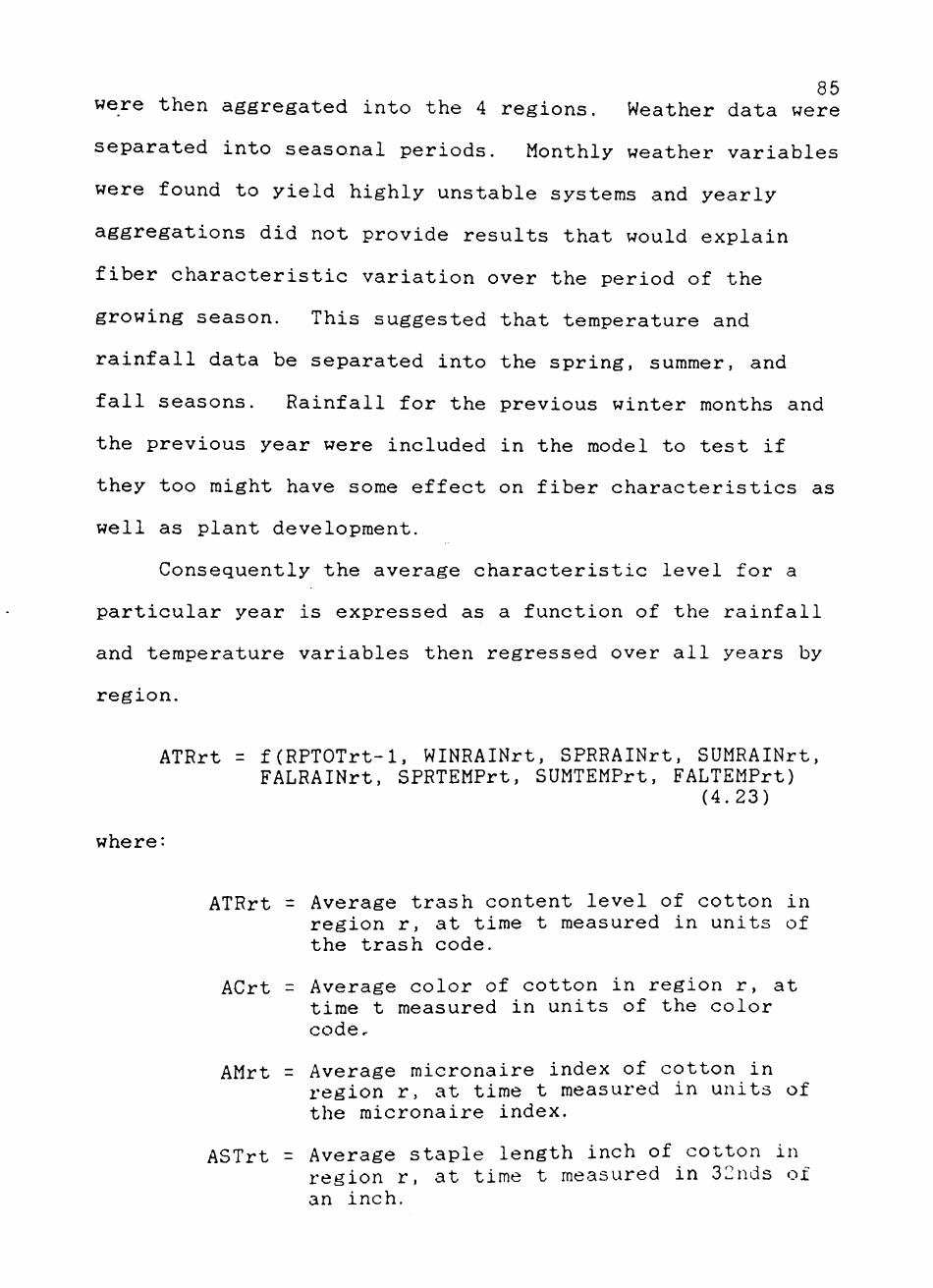
INTERCEPT RAINFALL PREVIOUS TOTAL SPRING TEMPERATURE FALL TEMPERATURE WINTER RAIN SPRING RAIN TIME

9.818 0.664 0.713 3.882

-2.021 0.803 1.245

1. 400 0. 162 0. 160 0.618 0. 136 0. 163 0. 080

7. 02 4. 10 4. 48 6.28

-14.91 4.94 15. 50


System Weighted Mean Squared Error: 0.926 1890 Degrees of Freedom Coefficient of Determination: 0JL8

139

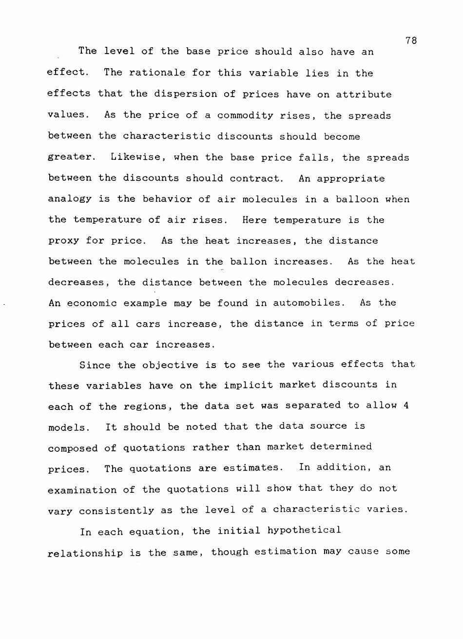
Table 5.9. Characteristic Specific Supply: Mid-South Average Tra,c h _ _ _ _ ^ INTERCEPT SPRING TEMPERATURE SUMMER TEMPERATURE WINTER RAIN SPRING RAIN SUMMER RAIN FALL RAIN um

7.772 -1. lE-10 -1.6E-10 -3.8E-7 7.6E-7 1.4E-6 7.9E-8

-1.2E-6

0. 028 1.8E-11 6.8E-12 1.5E-7 6.OE-8 7.4E-7 2.8E-8 6.5E-8

137.16 -6. 05 22.78 -2.55 12.69 1.92 2.80

-17.76 Coefficient of Determination: 0.38 Lambda: 5.0

Average Color



INTERCEPT SPRING TEMPERATURE SUMMER TEMPERATURE WINTER RAIN SPRING RAIN SUMMER RAIN FALL RAIN TIME

0.702 -1. 3E-10 1.7E-10

-3.6E-6 7.8E-7 1. OE-5 4.OE-7 3.3E-6

0. 041 1.8E-11 1.3E-11 2.7E-7 1. lE-7 1.3E-6 4.7E-8 1.lE-7

17. 12 -7. 42 13.72

-13.30 7.29 8. 32 8.50

31. 14 Coefficient of Determination: Q. 51 Lambda: 4.96

Parameter Variable Estimate INTERCEPT 35.761 SPRING TEMPERATURE -25.983 WINTER RAIN -0.870 SPRING RAIN -0.535 FALL RAIN -0.295 TIME -0.807 Coeffici^^nt of Determination: 0.£D

Standard Error 0. 116 14.790 0. 043 0. 112 0. 060 0. 021

Lambda: -1.

t-Value 308.28 -1.76

-20.42 -4.78 -4.92 -38.43

, 17

i;o




INTERCEPT RAINFALL PREVIOUS TOTAL SPRING TEMPERATURE WINTER RAIN SPRING RAIN FALL RAIN

4.981 7.796

-23.676 0.283

-0. 133 0.352

0. 497 0.497 2.814 0. 033 0. 072 0. 045

34.35 15.69 -8.41 8.58

-1.85 7.82

Coefficient of Determination: 0.23 Lambda: -Q. 71

Average Strength Parameter Standard

Variable Estimate Error t-Value INTERCEPT RAINFALL PREVIOUS TOTAL SPRING TEMPERATURE FALL TEMPERATURE SUMMER RAIN FALL RAIN TIME

25.264 -0.002 0. 030

-0.049 -0.027 -0. 017 0. 058

Coefficient of Determination: 0. 16

0. 389 0. 001 0. 003 0. 004 0. 007 0. 004 0. 003

Lambda:

64. 95 -4.23 10. 00

-12.25 -3.86 -4.25 19.37

1. 08

System Weighted Mean Squared Error: 4310 Degrees of Freedom Coefficient of Determination: 0.86

0.87

141

Table 5.10. Characteristic Specific Supply: Average Trash

Southwest

Variable INTERCEPT RAINFALL PREVIOUS TOTAL SUMMER TEMPERATURE FALL TEMPERATURE WINTER RAIN SPRING RAIN SUMMER RAIN FALL RAIN nuE

Parameter Estimate

2 . 9 6 5 - 0 . 0 2 6

0. 129 - 0 . 1 0 6

0. 119 - 0 . 105

0. 104 0. 171 0. 129

Standard Error 0. 138 0. 003 0. 013 0. 014 0. 015 0. 012 0. 008 0. 006 0. 006

t - V a l u e 2 1 - 8

9 - 7

7 - 8 13 28 2 1

49 67 92 57 93 75 00 50 50


Average Color



INTERCEPT WINTER RAIN SPRING RAIN FALL RAIN UhE

8. 6 1 1 1. 815

- 1 . 7 2 8 - 3 . 9 0 5 - 3 . 4 9 1

0 . 2 3 8 0. 098 0. 181 0. 114 0. 166

36. 18 18. 52 -9. 55 34.25 21. 03

Coefficient of Determination: Q.63 Lambda: -Q, 04

Average Staple Length



INTERCEPT WINTER RAIN SPRING RAIN SUMMER RAIN

29.970 0.989 -0.712 1.756

0. 095 0. 057 0. 069 0. 060

315.47 17.35

-10.32 29. 27


142


Variable INTERCEPT RAINFALL PREVIOUS TOTAL WINTER RAIN SPRING RAIN SUMMER RAIN FALL RAIN TIME

Parameter Standard Estimate Error t-Value 3.867 12.585 -4.6E-5 -0.037 0. 080

-0.063 0. 353

0. 012 1. 986 1.5E-5 0. 002 0. 008 0. 004 0. 024

322.25 6.34

-3. 01 -14.98

9.46 -17.00 14.65

Coefficient of Determination: 0.51 Lambda: -1.80

Average Strength

Variable INTERCEPT SPRING TEMPERATURE FALL TEMPERATURE WINTERS RAIN SPRING RAIN FALL RAIN TIME

Parameter Estimate 21.807 0. 039

-0.040 0. 116 0. 046

-0. 049 0. 120

Standard Error 0. 136 0. 002 0. 002 0. 015 0. 007 0. 003 0. 002

t-Value 160. 35 20. 10 -19.90

7. 73 6.37

-14. 40 52. 86

Coefficient of Determination: 0.68 Lambda: 1. 10

System Weighted Mean Squared Error: 0.95 5143 Degrees of Freedom Coefficient of Determination: 0.74

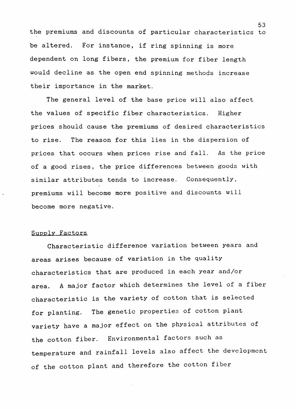
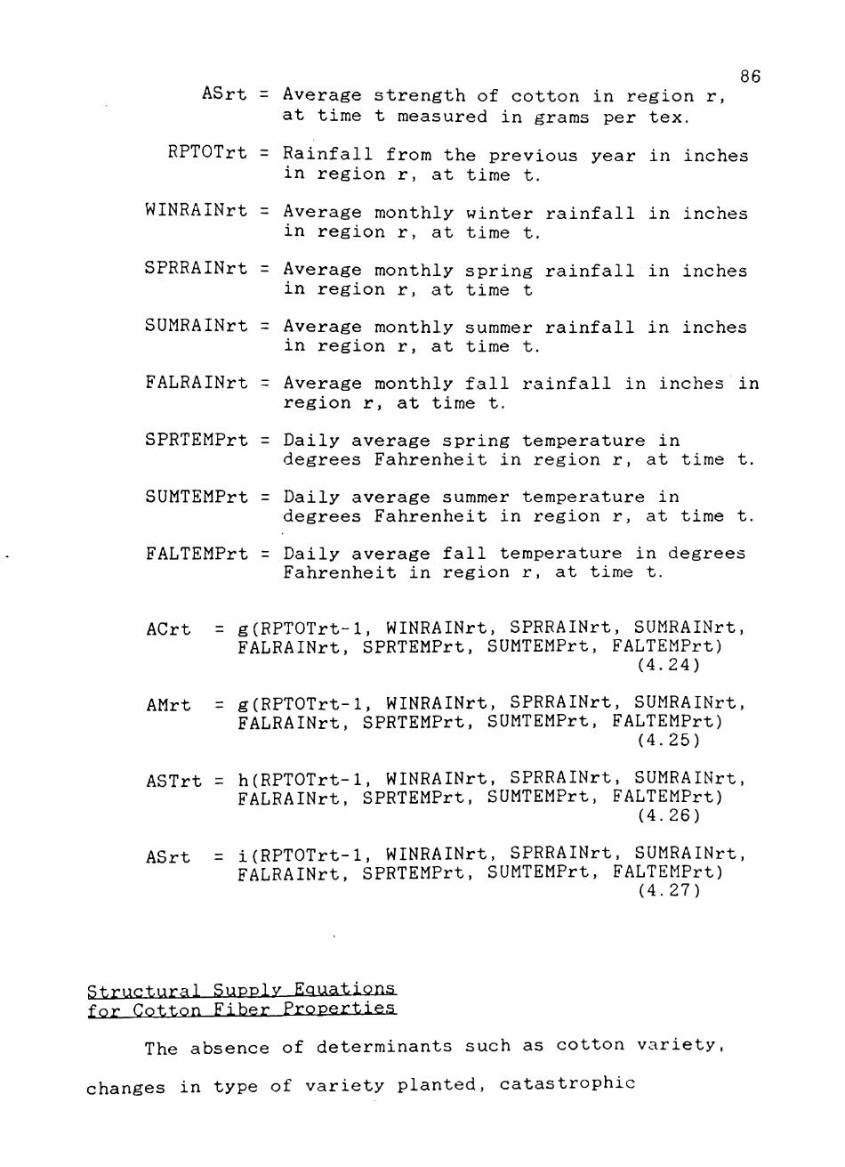
143

Table 5.11. Characteristic Specific Supply; Average Tra.- h

West

Variable INTERCEPT RAINFALL PREVIOUS TOTAL WINTER RAIN SPRING RAIN FALL RAIN TIME

Parameter Estimate


3. 055 0. 056

-0.382 0.999 0.306

-0.249

0. 060 0. 017 0. 019 0. 038 0. 014 0. 021

9? 50. »^ 3.36

-20. 11 26.29 21.86

-11. 86 Coefficient of Determination: 0.51

Average Color Parameter

Variable Estimate

Lambda: 0.34


INTERCEPT RAINFALL PREVIOUS TOTAL SPRING TEMPERATURE SUMMER TEMPERATURE FALL TEMPERATURE WINTER RAIN SPRING RAIN SUMMER RAIN FALL RAIN TIME Coefficient of

Average Siaple

Variable INTERCEPT SPRING RAIN TIME Coefficient of

Determinat

Length

1.248 6.8E-5

-1. OE-4 2.lE-5 2.lE-5 0. 003 0. 018 0. 015 0. 008 0.001

ion: 0.79

Parameter Estimate 34.367 1.403

-0.631 Determination: 0.26

0. 038 1.OE-7 4.9E-6 3.5E-6 3.OE-6 0. 001 0. 001 0. 002 0. 001 4.7E-5

Lambda: 2.

Standard Error 0. 140 0. 102 0. 129

.Lambda: -o,

33. 03 6.78

-21. 44 6. 06 6. 80 5. 75 12.21 9.55 12. 97 30.97

25

t-Value 245.48 13.71 -4. 89

14

144




INTERCEPT RAINFALL PREVIOUS TOTAL SPRING TEMPERATURE SUMMER TEMPERATURE FALL TEMPERATURE WINTER RAIN SPRING RAIN SUMMER RAIN FALL RAIN TIME

4.581 l.OE-4 1.7E-4 4.6E-5 3.3E-5 0. 004 0. 016 0. 022 0. 007 0. 001

0. 049 1.3E-5 6.6E-6 4.8E-6 4.lE-6 0. 001 0. 002 0. 002 0. 001 6.3E-5

v7 c. . KJ ^

7.61 -25.00

9. 59 7.91 6.36 8. 41 10.74 8.94

23.64 Coefficient of Determination: 0.74 L^mM^J Zuu2A.

Average Strength

Variable INTERCEPT RAINFALL PREVIOUS TOTAL SPRING RAIN SUMMER RAIN FALL RAIN TIME

Parameter Estimate 23.987 7.765 0 -0 0 -2

598 012 022 255

Standard Error 0. 088 0. 366 030 001 002 098

0 0 0 0

t-Value 272 21 20 -10 13

-22 Coefficient of Det.erminat i on: 0.54 [h mb'1- : -0.72

System Weighted Mean Squared Error: 3350 Degree of Freedom Coefficient of Determination: 0.63

0.89

89 24 13 26 46 96

145 foliage of the cotton plant more completely than would a

freeze.

Greater rainfall in the winter months decreased the

average trash levels in the mid-South, Southwest, and West,

though no interpretation is offered here for this phenomena

except that more winter rain might be a forerunner of other

weather variables associated with higher trash levels.

High spring rains were associated with increased levels of

trash in the Southeast, mid-South, and West, indicating

that increased amounts of vegetative matter were produced

because of the increased water. This parameter estimate

was negative in the Southwest, which was unexpected,

especially when the Southwest is a region where cotton is

predominantly stripped. Increased fall rains were positive

in all regions of the country, and had their greatest

impacts in the drier areas of the Southwest and West. Over

time, other things equal, the trash level of cottons in the

Southeast and Southwest increased while those in the West

and Mid-South decreased; no reason for these trends is

directly discernable.

Color. Rainfall from the previous year was effective

in raising the color level in the Southeast and West. As

rainfall increases in the Southeast, the color of the 0. 07

following years crop falls (-1.903*RPTOT ) while it 2.25

tends to rise in the West (0.0000657*RPTOT ). Temperature levels were significant in the West while

146 spring and summer temperature levels were significant in

the mid-South production areas. Temperature was not a

determinant of color in either the Southeast or Southwest.

Winter rainfall increased the color of cotton in the

mid-South, Southwest and West and decreased the color of

cotton in the Southeast. Spring, summer, and fall rainfall

increased the color levels of mid-South and Western

cottons. In the Southeast, spring rains lowered color

levels, while rains that occurred close to harvest

increased the color readings. Spring and fall rains

decreased the color levels in the Southwest. While higher

rainfalls are generally associated with increases in the

color levels of cottons, the amounts of dryland cotton in

the Southwest provide an explanation of this occurrence.

Higher levels of rainfall aids boll development, providing

a higher percentage of fiber in the cotton when classed.

Over the study period, the color levels of cottons in the

raid-South and West have fallen, while those in the

Southeast have risen, other things equal. Time was not

found to have an effect on color in the Southwest.

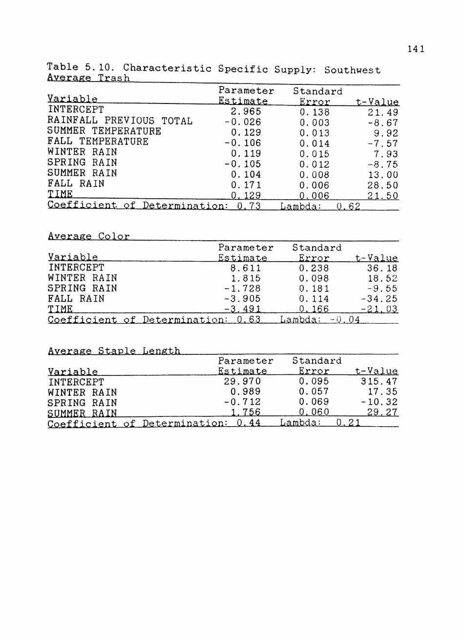
Staple length. The most notable weather related

information about staple length is the dearth of variables

that affect the length of cotton fibers and the small

effects of those variables that are significant. Previous

years rainfall was significant and positive in the

Southeast. Spring temperature had a negative effect on

-h 1 . 147

staple m the Southeast and the mid-South. The coefficient

for spring temperature in the mid-South was very large

(-25.983), but the exponent for the variable was very small

(-1.17). Consequently, the average effect of spring -1. 17

temperature was -25.983*SPRTEMP . An explanation of

the negative signs in these regions is found in the

negative signs for spring rainfall.

The coefficient for spring rainfall was also negative

in the Southwest, but was positive in the West. However,

since the average amount of rainfall for the spring in the

West is 0.091 inches with an exponent of -0.14, little

effect is produced by the variable. Summer and fall

rainfall variables were positive except in the Southeast

where increases in fall rainfall were associated with

shorter fibers. While the effect is slight, it is probably

due to the increased amount of ginning required to separate

the moist trash particles. Time was significant in the

Southeast and West. In the Southeast, fibers were becoming

longer over time and shorter in the West, though effects

were small in both regions.

Staple length is primarily determined by the variety

of the cotton that is planted. This is seen by the

combination of the sparsity of significant variables and by

an examination of the intercept terms. For the Southeast,

mid-South, Southwest, and West, the intercept terms were

34.7, 35.8, 30.0 and 34.4, respectively. The period

148

average means were 34.7 in the Southeast, 35.0 in the Mid-

South, 29.4 in the Southwest, and 35.1 in the West.

Micronc^jre. Like staple length, micronaire appears to

be predominantly determined by variety; i.e., the

intercepts are very close to the regional averages. The

intercept for micronaire in the Southeast is 4.7 while the

average micronaire was 4.5. The mid-South had an intercept

of 5.0 and an average of 4.4. The Southwest and West had

intercepts of 3.9 and 4.6 while their respective means were

3.9 and 4.3.

Unlike staple length, micronaire had many significant

weather variables. Rainfall was negatively correlated in

the heavy rainfall Southeastern region, and for the mid-

South and Southwest in the Spring. However, in both

regions the effect of the precipitation was very small.

For instance, in the Southwest, spring rainfall affected -1.80

micronaire development at a rate of -0.037*SPRRAIN

The decline in the micronaire value due to spring rain is

probably due to the delay in planting and the subsequent

shortening of the growing season. Summer rainfall did not

affect the micronaire level in the mid-South but had a

positive effect in the Southwest and West. Fall rain was

positively related to micronaire development in all regions

except the Southwest.

Study results indicate that temperature was more

likely to have an effect in the Southeast and West. Cotton

149 plants require a minimal temperature for crystalline cell

wall development to occur but this minimum is apparently

not a problem in the 4 production regions of the country.

In the Southeast, spring temperature was positively related

to micronaire while summer temperature and micronaire had

an inverse relationship. The negative sign for summer

temperature could reflect periods of moisture stress in the

region. The relationship between spring and summer

temperatures in the West is the opposite of that in the

Southeast because moisture stress is unlikely to occur

because of the large amount of the crop that is under

irrigation. The trend variable indicated that, other

things equal, micronaire levels have increased in the

Southwest and West while declining in the Southeast. The

decline in the Southeast may be intentional on the part of

producers since penalties for high micronaire readings have

begun to increase, and because Southeastern cottons had the

highest micronaire levels over the period of all 4

production regions.

Strength. Strength was affected in all regions by the

levels of rainfall, although the effects varied across

regions. In the West, increases spring and fall rainfall

levels increased the strength of the cotton while increases

in summer rainfall had the opposite affect. Since the

coefficient for this variable was -0.12 and the mean

rainfall level in this region was 0.40 inches, the impact

150 of the variable on the level of strength is small. Fall

rainfall in the Southwest and mid-South also decreased the

strength level of cotton fibers which could be due to fiber

deterioration in the field or fiber damage due to moisture

levels which occur in the ginning process. Spring rain

increased the strength levels of fiber in the 3 regions

where the variable was significant, suggesting that initial

plant development may have some determination of the fiber

strength. Fall rain was negatively related to fiber

strength in the Southwest f=ir\d mid-South as expected, but

was positively related to fiber strength in the the West.

While the affect was again very small, it was not expected.

The relationship between fiber strength and

temperature displayed an interesting relationship. In the

Southeast, all temperature levels in all periods except

summer were positively related to strength. In the

Southwest and mid-South, summer temperatures had no effect

while higher spring temperatures were related to stronger

fibers and higher fall temperatures were associated with

weaker fibers. Since the strength level of fibers is

usually determined before the autumn months, higher

temperatures at this time reflect the necessity and effects

of defoliants and dessicants on trash and the amount of

ginning that the cotton requires. In the West, temperature

had no statistically significant effect on the strength of

151 the cotton fibers. Consequently, the pattern established

was that temperature has a smaller effect on cotton fiber

strength the farther west the production area is located.

The trend variable time indicated that fibers were becoming

stronger in the Southeast, the mid-South, and the Southwest

while those in the West were becoming slightly weaker over

the period, other things equal.

CHAPTER VI

SUMMARY AND CONCLUSIONS

Summary

Price is the messenger that relays the information

generated by the participants of the market. Hedonic

theory adds content to price information. It provides a

method for analyzing markets which are not perfectly

competitive because of product differentiation. When

characteristic differences between goods yield price

differences, hedonic theory is an effective tool for

discovering the value of product characteristics.

Characteristic prices perform the same functions as

product prices. When the demand for a particular

characteristic rises, the price of the characteristic

will also rise, other things equal. When the supply of a

characteristic rises, the price of the characteristic

will fall, ceteris paribus. Knowledge of characteristic

values adds information to the marketplace. Producers

and buyers are aware of the value of product attributes.

This information encourages efficiency because producers

are able to more effectively satisfy the needs buyers by

supplying characteristics that buyers wishes to purchase.

This study used the hedonic discount technique to

derive characteristic values of cotton. Initially, a set

152

of 11 equations were estimated that expressed cotton

price differences as functions of characteristic

differences. Characteristic slope shifters were included

to account for characteristic value variation between

regions. Regional intercept shifters were included to

account for price differences due to location and other

factors. All signs were expected and coefficient

magnitudes were rational.

While this study concentrated on cotton, it is

believed that the hedonic discount technique is readily

applicable to any product. A base set of characteristics

would be defined for a good, and the price of this set of

characteristics would become the base price. Product

price differences from the base would then be expressed

as a function of the characteristics to derive the

characteristic values.

Discounts for trash were found to be more severe in

areas where cotton trash levels were low. Study period

trash discount means ranged from 3.93 cents per pound in

the West to 2.59 cents per pound in the Southwest. An

examination of the trash discount showed that penalties

for the last 5 years of the study were higher than those

in the first 6 years. This indicates that cotton buyers

are demanding cleaner cottons. This is expected because

of the adoption of open end spinning techniques. Open

153

end spinning technologies are more trash sensitive than

ring spinning methods.

Color discounts had a significant amount of

variation between regions. Discounts were generally

lower in the Southwest (2.72 per pound) and higher in the

Southeast (3.76 per pound). While discounts varied

between regions, regional discounts tended to follow the

same trends over time. They were relatively low during

the 1970's and higher in the 1980's. Buyers have

revealed preferences for increasingly whiter fibers.

Staple length premiums also illustrated the

influences of new spinning technologies. Staple length

is of greater importance to ring spinning technologies

than to open end spinning. As a result, premiums for

staple length declined over the study period. In fact,

staple premiums exceeded study period premiums means in

only 1 year of the last 5 years of the study (1982).

Staple length premiums were slightly higher in the

Southwest than in other regions. This suggests that

premiums are greater in the areas of the country where

long fibers are more scarce.

Micronaire was split into low, medium, and high

ranges to duplicate the manner in which current discounts

are assessed in the spot markets. Discounts for low

micronaire diminished over time while discounts for high

micronaire generally rose. This result indicates that

154

cotton buyers are presently demanding finer fibers. It

should be remembered that buyers are not necessarily

demanding low micronaire fibers. Micronaire is a measure

of fiber fineness and maturity. Ideally, buyers would

prefer fine, mature fibers. Methods which separate the

components of micronaire are currently available and will

become a part of the grading process when they are

economically feasible.

Strength premiums did not exhibit any general

trend. The absence of a definite pattern maybe due to 2

factors. First, strength is not generally reported when

cotton is sold. This means that buyers are not certain

of the strength levels of the cotton they purchase.

Second, increased awareness of fiber strength values ha.s

encouraged cotton producers to plant varieties which

yield stronger fibers. The increased supply of strong

cotton may have diminished strength premiums in the later

years of this study. More precise information concerning

strength premiums will become available when strength is

widely reported at points of sale. Currently, this takes

place only in the Southwest region.

A study of characteristic price flexibilities

indicated that cotton prices are not very responsive with

respect to characteristic levels. The characteristic

which generally had the greatest impact on cotton prices

was micronaire. Cottons with micronaire levels which

155

fell into the high or low ranges were significantly

discounted. Staple length also significantly affected

cotton prices though this impact diminished as the study

period progressed. An examination of the price

flexibilities revealed that cotton prices were

approximately 3 times more responsive to trash than to

color. This indicates that nonlint content is currently

more important to cotton buyers than fiber color.

Characteristic demand equations showed the

characteristic specific demand for cotton fiber

attributes which is not due to general market forces.

These equations also illustrate that characteristic

values are functions of other characteristics in a

particular lot of cotton.

Trash was often influenced by color, its counterpart

in the 2 digit grade code. Additional units of color

increased the severity of the trash discount. Micronaire

and strength diminished the trash discount, though

strength had smaller impacts on the trash discount.

Increases in the proportion of open end spindles to ring

spindles caused the penalty for trash to increase. Open

end spinning technologies do not tolerate nonlint content

as well as ring spinning techniques. The effect of this

variable was most pronounced in the West. Western cotton

is often exported to the open end spinning intensive

countries of the Far East. Increases in the base pri<

156

. C (.'

157 increased the severity of the trash discount in all areas

of the country except the West.

Color was not often affected by additional units of

trash, which may reflect restrictions imposed by the data

set. Likewise, strength had a significant effect on

color discounts only in the mid-South. Increases in the

base price increased color discounts, as expected, with

the largest impacts occurring in the mid-South and the

Southwest. Effects in the other regions were very

similar. The increased adoption of open end spinning

increased color discounts. This again reflects the

differences in characteristic demand between the 2

spinning technologies. Again the largest impact of the

technology variable on color discounts was in the West.

Staple length premiums were affected by micronaire.

Parameter estimates of the impact of micronaire on staple

premiums were very similar in all regions. Open end

spinning had an inverse relationship with staple

premiums. Staple length is not as important to open end

spinning as it is to ring spinning. Trash and color were

conspicuous by their absence in the staple length

equations. Data limitations are the suspected cause of

this phenomena. Base price increases caused staple

premiums to increase but the effects were small.

Low micronaire discounts were lowered by increases

in micronaire, as expected. Increases in micronaire

levels cause the discount for high micronaire to

increase. Since open end spinning technologies demand

finer fibers, its relationship to low micronaire was

direct and its relationship to high micronaire was

inverse. Higher base price increased micronaire

discounts for both high and low micronaire cotton. High

micronaire discounts were more often increased by

components of the grade code than low micronaire, though

the reason for this is not clear. Strength and staple

length had little impact on either.

The strength premium was often affected by color but

not trash. Micronaire also had a significant impact on

strength premiums. Increases in the base price brought

about increases in strength premiums and had the same

magnitude in all regions. Curiously, the technology

variable was not significant in any region. This may be

due to the fact that strength is often only reported at

points of sale in the Southwest.

In the characteristic supply equations, trash was

often a function of both rainfall and temperature

variables. It was concluded that rainfall generally

enhances foliage development thereby increasing trash

levels, though coefficients for all rainfall variables

were not positive. High temperatures in the fall months

were associated with lower trash levels. Higher

temperatures at this time apparently encourage the use of

158

dessicants and defoliants which may decrease trash more

effectively than a freeze.

High levels of rainfall during the growing season

were generally associated with higher levels of color

except in the Southwest. Preplant rainfall was also

associated with higher color levels. Temperature had

significant impacts in the West and mid-South with the

impacts generally greater in the earlier periods of the

growing season. Color levels in the mid-South and West

are decreasing with respect to time while those in the

Southeast are rising, other things equal. The Southwest

did not establish a statistically significant pattern for

color with regard to time.

Staple length was notable for the sparsity of

weather variables that affected it, and the small effects

of the variables that were significant. Staple length in

the Southeast was,' on average, impeded by high levels of

rainfall occurring during fiber development periods. All

other regions had positive coefficients for rainfall in

these periods. Variation in temperature had little

impact on staple length development. It is possible that

cotton production areas generally exceed minimum

temperature requirements for staple length thereby

negating the significance' of temperature.

Micronaire was affected by many weather variables,

though parameter estimates were small. Curiously, spring

159

rainfall decreased micronaire levels, though the impacts

were very small. The negative coefficient may be due to

delays in planting which shorten the growing season.

Summer rainfall was important in the moisture deficient

areas of the Southwest. Summer temperature was a factor

only in the Southeast and West. Crystalline cell wall

development requires a minimum level of temperature but

this is generally not a problem in the summer months. In

fact, it is possible that high temperatures might induce

moisture stress. Over time, micronaire levels have

increased over the study period in the Western half of

the United States and have fallen in the Southeast.

Southeastern producers may be intentionally lowering

micronaire levels because penalties for high micronaire

have increased and the Southeast has historically

produced high micronaire fibers.

Spring rainfall increased strength levels while fall

rainfall often decreased them. This might reflect fiber

deterioration and would also explain the influence of

color on strength premiums. Temperature displayed

greater impacts on strength in the Southeast. The

significance of temperature diminished as the production

area moved westward. In fact, variations in temperature

had no effects on fibers in the West. The time variable

indicated that fibers were becoming stronger in all areas

except the West.

160

161 Conclusipr^s

The results of this study demonstrate that there is

a functioning market for cotton fiber characteristics.

However, the price information generated in that market

is not obvious to participants in the market at present

except through analyses such as that in this study. At

present, fiber strength and length uniformity levels are

reported only for cottons produced in the Southwest.

Since market participants in other regions are unaware of

fiber strength levels, no premium for this characteristic

is quoted even though buyers prefer stronger fibers.

Even though strength and uniformity measures are

available in the Southwest, price premiums and discounts

are not reported even in these markets to facilitate

marketing functions through price information.

However, there is a growing recognition of the need

to understand the values of fiber characteristics.

Buyers know that fiber characteristics impact the value

of their products and the efficiency with which they may

be produced. However, the marginal cost of additional

characteristics is not known. Cotton producers know that

fiber characteristics affect the monetary value of their

crops, but the marginal revenue generated by increases in

specific fiber qualities is not known for several

characteristics.

162 The characteristics model constructed in this paper

is useful because it presents an alternative to the

current method of determining premiums and discounts.

Rather than relying on judgement alone to estimate

premiums and discounts for cottons with various

characteristic combinations, the values may be determined

through statistical procedures. Furthermore, the model

provides the means to analyze the market functioning

ex-ante rather than ex-post.

In addition, the precision of characteristic price

signals is enhanced because each attribute has a value of

its own. Producers can determine the additional revenue

which may be earned from a 1 unit increase or decrease in

each particular attribute. Buyers can measure the change

in cost that arise from purchasing cottons with

additional units of a characteristic. This cost can be

compared to the value marginal product of an attribute to

determine optimal characteristic selection.

While this model represents an improvement in

characteristic valuation, problems still exist. The

principal problem is that some fiber characteristics are

not evaluated prior to sale. Buyers and producers cannot

completely estimate the value of cottons because all

pertinent characteristic levels are not reported. This

impediment will be removed with the implementation of

High Volume Instrument (HVI) fiber evaluation systems.

163 HVI evaluates cotton characteristics, including strength

and length uniformity, and reduces the amount of human

error which may occur during the grading process. This

will increase the information available to market

constituents.

The results obtained for the characteristic specific

demand equations confirmed expectations of characteristic

interaction on characteristic values. Statistical

analysis revealed a significant degree of reliability of

the results. However, the efficiency of the study was

impeded to a small degree by the data. In the spot

quotations, values of a characteristic do not vary in any

systematic pattern as the amount of the characteristic

varies within a given year. The absence of systematic

variation of characteristic values inhibits the

efficiency which characteristic specific demand may be

discovered. This is also thought to be the cause of the

lack of statistical significance of some regressors in

these equations. In spite of these limitations, the

estimates derived and presented here are believed to be

the most accurate currently available.

The characteristic specific supply equations

represent an attempt to judge the impact of environmental

factors on characteristic levels. Since research has

only recently began in this area, the results generated

in this study are thought to be the most comprehensive to

date. To provide a definitive study of all factors in

all United States production regions, a large number of

variables would be required. This would be a task of

considerable dimension.

While the results of the characteristic specific

supply equations do not represent the final word on this

subject, they do illustrate the effects of the

environmental variables when other things are equal.

Parameter estimates illustrate the impacts of rainfall

and temperature in all areas of the country. While this

information is not complete, it is an addition to the

information presently available. The impacts of rainfall

and temperature on cotton characteristics in all areas of

the country are now quantifiable. Multi-disciplinary

research teams of economists and agronomists may be

needed for definitive supply response quantification.

Suggestions for Further Research

The greatest obstacle to further research in cotton

characteristic pricing is the availability of a larger

and more detailed data base. Present research must be

conducted with price information provided by the spot

quotations. Price data from actual transactions with

characteristic information on strength, fineness.

164

maturity and length uniformity would enhance modeling

results from future studies.

Other methods could also be applied to

characteristic forecasting. For example, since the

impacts of weather variables are probably a function of

the state that the plant is in when the variable occurs,

a Markov chain model could be an effective way to

approach the problem.

For research on characteristic analysis, it should

be noted that hedonic theory is quite malleable. There

are very few restrictions that constrain the researcher.

As a result, if the hedonic theory by Rosen is used, it

may be possible to add quantity variables to the supply

and demand equations to form a simultaneous equation

system. Quantity variables would be necessary because

general supply and demand forces affect the

characteristic prices defined in Rosen's theory. These

procedures are certainly desirable though attempts to use

them have not been successful to this point.

The next step in the development of the hedonic

model of the cotton market would be to develop a method

for estimating the price for cotton that has the base set

of characteristics. This would allow the results that

have been derived in this paper to be combined to

formulate a method for ex-ante estimation of the prices

as well as the values for all fiber characteristics.

165

BIBLIOGRAPHY

Bartick, Timothy J., "The Estimation of Demand Parameters in Hedonic Price Models,'" Journal of Political Economy. 95,1(1987): 81-88.

Bowman, Kenneth R., and Don E. Ethridge, "Prices Paid By Textile Manufacturers for Cotton Fiber Properties," 1987 Beltwide Cotton Research Conference Proceedingp. , Cotton Economics Conference, 1987, 446-448.

Brown, James N., and Harvey S. Rosen, "On the Estimation of Structural Hedonic Models," Econometrica. 50(May 1982): 765-768.

Brorsen, Wade B., Warren R. Grant, and Edward M. Rister, "A Hedonic Price Model for Rice Bid/Acceptance Markets," American Journal of Agricultural Economics. 66(1984): 156-163.

Carl, E. K. , R.L. Kilmer, and L.W. Kenny, "Evaluating Implicit Prices for Intermediate Products," American Journal of Agricultural Economics. 65(1983): 592-95.

Crawford G.L., and L.P. Gabbard, "Relation of Farm Prices to Quality of Cotton," Tex. Agr. Exp. Sta. Bulletin No. 383, July 1928.

Deussen, Helmut, "Some Thoughts on the Role of Cotton in New Spinning Technologies," Schlafhorst Dokumentation No. 10, presented to Cotton Spinners and Growers Conference, Lubbock, Texas 1984.

Dhrymes, Phoebus J. "On the Measurement of Price and Quality Changes in Some Consumer Capital Goods," American Economic Review. 57(1967): 501-518.

Dutta, M., Econometric Methods. South-Western Publishing Co., Cinn., Ohio, 1975.

Eastwood, David B., John R. Brooker, and Danny E. Terry, "Household Nutrient Demand: Use of Characteristics Theory and a Common Attribute Model," Southern Journal of Agricultural Economics. 18,2(1986): 235-243.

Ethridge, Don E., and Bob Davis, "Hedonic Price Estimation for Commodities: An Application to Cotton," Western .Journal Agricultural Economics. 7,2(1982): 293-300.

166

167

Ethridge, Don E., and Kenneth H. Mathews, "Reliability of Spot Cotton Quotations for Price Discovery in the West Texas Cotton Market," Ag. Econ. Dept., Texas Tech Univ. College of Ag. Sci. Pub. No. T-1-212, Aug 1983.

Ethridge, Don E., and Jarral T. Neeper, "Producer Returns from Cotton Strength and Uniformity: An Hedonic Approach," Southern Journal of Agricultural Economics, 19,(l)(1987): 91-97.

Ethridge, Don E., Dale L. Shaw, and John E. Ross, "An Evaluation of the Impact of Instrument Test Line Values on Cotton Marketing and Use: Progress Report," CED Working Paper, Economic Research Service, USDA, Aug. 1977.

Ethridge, Don E. , Randy Sudderth, and Mark Moore, '"A Model for Cotton Variety Selection with Yield and Quality Considerations,"' 1983 Beltwide Cotton Research Conference Proceedings. Cotton Economics and Marketing Conference, Jan. 1983 : 251-253.

Fisher, Franklin M., and Karl Shell, "Taste and Quality Change in the Pure Theory of the True Cost of Living Index," Value. Capital, and Growth: Essays in the Honor of Sir John Hicks. Ed., J.N. Wolfe. Edinburgh: University of Edinburgh Press 1968.

Goodman, Allen C., "Hedonic Prices, Price Indices and Housing Markets,"" Journal of Urban Economics . 5(1978): 471-478.

Griliches, Zvi, Ed. Price Indexes and Quality Change. Harvard University Press, Cambridge, Mass. 1971.

Hembree, Joel F., Don E. Ethridge, and Jarral T. Neeper, "Market Value of Fiber Properties in Southeastern Textile Mills," Paper presented at the 1985 Cotton Textile Conference, New Orleans, National Cotton Council Jan. 1985.

Horak, John D., "Cotton Pricing According to Fiber Properties," Natural Fibers Economic Research, The Univ. of Texas at Austin, Research Rep. No. 110, Dec. 1976.

Howell, L.D., and Joel F. Hembree, "Farm Prices of Cotton Related to Grade and Staple Length in the United States,"' USDA Technical Bulletin No. 493, Jan. 1936.

168

Howell, L.D. , and Leonard J. Watson, ""Cotton Prices in Relation to Cotton Classification Service and to Quality Improvement,"' USDA Tech. Bui. No. 699, Oct 1939.

Jones-Russell, Eluned, T.L. Sporleder, and Hovav Talpaz, "Fiber Characteristics Values by Major Spinning Technology,"' Cotton Economics and Marketing Conference Proceedings: 337-340, Las Vegas, Nev. Jan. 1986.

Jordan, Jeffrey L. , R.L. Shewfelt, S.E. Prussia, and W. C. Hurst, "Estimating Implicit Market of Quality Characteristics of Tomatoes," Southern Journal of Agricultural Eoononii , , 17,2(1985): 139-145.

Kinoshita, Tomio, "'Working Hours and Hedonic Wages in the Market Equilibrium,'" Journal of Political Economy. 95,6(1987): 1262-1277.

Ladd, George W. , and Veraphol Suvannunt, "A Model of Consumer Goods Characteristics,"" American Journal of Agricultural Eoonomin.c . 58,3(1976): 504-10.

Ladd, George W. , and Martin Zober, "'Model of Consumer Reaction to Product Characteristics," Journal of Consumer Research. 4(1977): 89-101.

Lancaster, Kelvin J. "A New Approach to Consumer Theory," Journal of Political Economics. 74(1966): 132-57.

Lancaster, Kelvin J. Consumer Demand: A New Approach. Columbia University Press, New York 1971.

Linneman, Peter, "Some Empirical Results on the Nature of the Hedonic Price Function for the Urban Housing Market,"" Journal of Urban Economics. 8(1980): 47-68.

Milon, J. W. , J. Gressel, and D. Mulkey, "'Hedonic Amenity Valuation and Functional Form Specification,'" Journal of r.and Economics. 6(1984): 378-87.

Neter, John, William Wasserman, and Michael Kutner, Applied Linear Regression Models. Richard D. Irwin Inc. Homewood, 111. 1983.

Newton, Franklin E., Samuel T. Burley, Jr., and Preston E. LaFerney, "'Does Cotton Price Reflect Use Value?,"' Textile Industries. 131(1967): 76-80.

169

Palmquist, Raymond B. , "'Estimating the Demand for the Characteristics of Housing," The Review of Economics and Stati.qt.ics. 66(1984): 394-403.

Paulson, W.E., and Joel F. Hembree, "Price-Quality Relationships in Farmer's Cotton Markets of Texas,"' Texas Agricultural Experiment Station Bulletin No. 501, Dec. 1934.

Perrin, Richard K. "The Impact of Component Pricing of Soybeans and Milk," American Journal of Agricultural Economics, 62(1980): 445-55.

Price, John B., "Future Fiber Requirements for Modern Spinning Technology," Texas Tech University, 1986.

Robinson, Jess A., Don E. Ethridge, Dale L. Shaw, and Clarence D. Rogers, "Market Impact Evaluation of Instrument Testing of Cotton: Progress Report," CED Working Paper, Economics Statistics and Cooperatives Service, USDA, May 1979.

Rosen, Sherwin, "'Hedonic Prices and Implicit Markets: Product Differentiation in Pure Competition," Journal of Political Economy. 82(1974): 34-55.

Spitzer, John, J., "A Primer on Box-Cox Estimation," Review of Economics and Statistics. 64(1982): 307-313.

Sporleder, Thomas, J. Haskell, Don E. Ethridge, and Robert Firch, "Who Will Market Your Cotton?," Texas Agricultural Extension Service D-1054, 1978.

Taylor, Fred, "Relation Between Primary Market Prices and Qualities of Cotton," USDA Bull. No. 457, Nov 24, 1916.

Triplett, Jack E. , "'The Economic Interpretation of Hedonic Models,"' Survey of Current Business. Jan. (1986): 36-48.

Triplett, Jack E. , and Richard J. McDonald, "'Assessing the Quality Error in Output measures: The Case of Refrigerators," Review of Income and Wealth, 23 (1977) : 137-156.

USDA, Cotton Market News; Southern and Western Review, Agricultural Marketing Service, 2/9/78, 2/9/79, 2/14/80,. 2/12/81, 2/11/82, 2/17/83, 2/16/84, 2/14/85. 2/13/86.

170 USDA, Summary of Cotton Fiber and Processing Test Results,

Agricultural Marketing Service Cotton Division, annual issues 1977-1985.

Waugh, Frederick V. , ""Quality Factors Influencing Vegetable Prices,"' Journal of Farm Economics, 19(1928): 185-196.

Wilson, William W. , '"Hedonic Prices in the Malting Barley Market," Western Journal of Agricultural Economics, 9(1984): 29-40.

Witte, Ann, D. Howard J. Sumka, and Homer Erekson, "An Estimate of Structural Hedonic Price Model of the Housing Market: An Application of Rosen's Theory of Implicit Markets," Econometrica, 47(1979): 1151-1173.

Zarembka,P. "Transformation of Variables in Econometrics," P. Zarembka, (ed. ), Frontiers in Econometrics. New York: Academic Press, 1974: 81-104.

Ziemer, Rod F., Wesley N. Musser, and R. Carter Hill, "Recreation Demand Equations: Functional Form and Consumer Surplus,"" American Journal of Agricultural Economics. (1980): 136-141.

APPENDIX

171

172

Table A.1 Hedonic Discount Equation Results for 1977 Parameter Standard

Variah! R Estimate Error t-value INTERCEPT DTR DTRRl DTRR3 DC DCRl DCR2 DST DLM DHM • DS R2 R3

0 . 6 4 3 - 3 . 0 0 2

0 . 8 7 6 2 . 133

- 1 . 135 - 2 . 4 7 8 - 1 . 064

0 . 9 9 0 - 5 . 4 4 4 - 3 . 1 8 5

0. 083 - 1 . 8 2 2 - 3 . 6 5 7

0. 173 0. 133 0 . 2 9 1 0 . 2 1 2 0. 143 0 . 2 0 7 0 . 2 3 5 0. 059 0 . 8 1 9 0 . 6 9 7 0. 026 0. 176 0. 217

3 . 7 1 - 2 2 . 5 3

3 . 0 1 10. 06 - 7 . 9 1

- 1 1 . 9 6 - 4 . 5 2 1 6 . 8 6 - 6 . 6 5 - 4 . 5 7

3 . 18 - 1 0 . 3 4 - 1 6 . 8 7

Coefficient of Determination: 0.94 F-Value: 478.08 Root Mean Squared Error: Q.98


Variable Estimate Error t-value INTERCEPT 0.101 0.327 0.31 DTR -4.350 0.271 -16.04 DTRRl 2.677 0.760 3.52 DTRR2 1.398 0.375 3.73 DTRR3 2.608 0.348 7.49 DC -1.837 0.176 -10.43 DST 1.278 0.136 9.41 DSTR3 -0.387 0.151 -2.57 DLM -6.025 1.057 -5.70 DHM -7.586 1.134 -6.69 DS 0.500 0.054 9.18 Rl -2.222 0.299 -7.42 R2 -2.223 0.260 -8.54 R2 -fi fi71 0.311 -18-23 Coefficient of Determination: 0.94 F-Value: 451.60 pnot Mean Squared Error: 1.41

173

Table A.3 Hedonic Discount Equation Results for 1979



INTERCEPT DTR DTRRl DTRR2 DC DCRl DCR2 DST DLM DHM • DS Rl R3

-1.601 -2.079 -1.216 -1.647 -1.686 -0.913 -1.616 0.783

-13.521 -2.260 0. 482 1. 027

-5.575

0.264 0. 171 0.503 0. 387 0.249 0. 493 0.499 0.900 0.582 1.342 0. 056 0.359 0.300

-6. 06 -12.20 -2. 42 -4.26 -6.78 -1.85 -3.24 8.75

-32.25 -1.68 8.55 2.86

-18. 62 Coefficient of Determination: 0.95 F-Value: 575.37 Root Mean Squared Error: 1.63

Table A.4 Hedonic Discount Equation Results tox 1960

Variable INTERCEPT DTR DTRRl DTRR2 DC DCRl DCR2 DST DLM DHM DS Rl R2 E3

Parameter Estimate -4.690 -3. 160 -2.260 -1.471 -3.316 -1. 358 -0.966 1.266

-15.757 -6.442 0. 340 4.682 3.320 -1.237

Standard Error 0 0 0 0 0 0 0 0 2 2 0 0 0

462 256 769 450 251 557 528 108 513 546 074 658 461

0.507

t - v a l u e - 1 0 - 2 1

- 2 - 3

- 1 3 - 2

15 35 94 27 19 44

- 1 . 8 3 1 1 . 6 9 - 6 - 2

4 7 7

-Z

27 53 6 1 12 20

Al. Coefficient of Determination: 0.90 F-Value: 278.14 Root Mean Squared Error: 2, 16

174

Table A. 5 Hedonic Discount Equation Results for 1981 Parameter Standard

Variable INTERCEPT DTR DTRR2 DC DCRl DST DSTR3 DLM DHM DS R3

Estimate -1.376 -3.721 -1.614 -3.664 -1.707 0.596 0.328

-6.914 -7.722 0.219

-2.937

Error 0.358 0. 199 0. 424 0.236 0. 495 0. 168 0. 194 0.777 1. 116 0. 075 0.361

t-value -3. 84

-18.72 -3.81

-15. 51 -3.45 3. 54 1.69

-8. 90 -6. 92 2. 94



Variable Estimate Error t-value INTERCEPT -1.794 0.305 -5.88 DTR -4.905 0.387 -12.66 DTRRl -1.327 0.626 -2.12 DTRR2 -2.425 0.594 -4.08 DTRR3 3.780 0.537 7.04 DC -3.049 0.325 -9.39 DCRl -1.338 0.553 -2.42 DCR2 -1.263 0.466 -2.71 DST 1.376 0.123 11.16 DLM -16.110 1.372 -11.74 DHM -5.223 1.632 -3.20 DS 0.204 0.071 2.87 B3 - 1 . 6 0 1 Q.471 - 3 . 4 0 C o e f f i c i e n t of D e t e r m i n a t i o n : 0. 95 F - V a l u e : 232 .97 Root Mean Squared Error: 1.28 ^

175


Variable Estimate Error t-value INTERCEPT DTR DTRRl DC DCR2 DCR3 DST DLM DHM DS • R3

-3. 186 -4.071 -1.501 -4.634 2. 437 1.234 0.244

-2.776 -7.741 0.974

-2.747

0. 451 0.311 0.743 0.357 0.612 0.514 0. 118 1.542 4. 159 0. 104 0.570

-7. 07 -13. 07 -2. 02

-12.97 3.98 2.40 2. 07

-1. 80 -1.86 9.33



Variable Estimate Error t-value INTERCEPT DTR DTRRl DTRR2 DC DCR2 DST DLM DHM DS R3

-2.820 -2.565 -1.337 -1.996 -2.768 -2.639 0.396

-6.950 -6.869 0.380

-2.477

0.479 0.289 0.707 0.511 0.286 0.645 0. 158 0.656 3. 026 0. 103 0,654

-5.89 -8.89 -1.89 -3.91 -9.68 -4. 09 2.51

-10.51 -2.27 3.69 -3.79

Coefficient of Determination: 0.94 F-Value: 237.62 Root Mean Squared Error:—1.80

176


Variable Estimate Error t-value INTERCEPT DTR DTRR2 DC DCRl DST DLM DHM R2 R3

-1. 468 -3.724 1. 574

-1.962 -2.839 0. 744

-5.636 -2.953 0.881

-1. 282

0.223 0. 181 0.451 0.278 0.607 0. 108 1.381 1.943 0.236 0.380

-6.59 -20.60

3.49 -7. 07 -4.68 6.91

-4. 08 -1.52 3.74 -3.37

Coefficient of Determination: 0.95 F-Value: 298.15 Root Mean Squared Error: 1. 11

Table A. 10 Hedonic Di.scount Equation Results for 1986 Parameter Standard

Variable Estimate Error t-value INTERCEPT DTR DTRRl DTRR2 DTRR3 DC DCRl DCR2 DCR3 DST DLM DHM R2 R3

0.208 -9.816 5. 882 7.752 6. 655 -8.227 3.375 5. 013 4.225 0.533

-5.897 -5. 132 -1.761 -2.539

0. 495 0. 568 0.843 0.805 0.649 1. 101 1.254 1. 177 1. 167 0. 148 1.340 1.795 0.579 0.625

0. 42 -17. 29 6.98 9.63 10.26 -7. 47 2.69 4.26 3.62 3.60

-4. 40 -2.86 -3. 04 -4. 06

Coefficient of Determination: 0.96 F-Value: 292.24 pnnt Mean Squared Error: 1.49

Date post:	18-Mar-2022
Category:	Documents
Upload:	others
View:	3 times
Download:	0 times

A MULTI-STAGE HEDONIC MARKET MODEL OF COTTON ...

Documents