A multilevel, level-set method for optimizingeigenvalues in shape design problems

E. Haber∗

July 22, 2003

Abstract

In this paper we consider optimal design problems that involveshape optimization. The goal is to determine the shape of a certainstructure such that it is either as rigid or as soft as possible.

To achieve this goal we combine two new ideas for an efficientsolution of the problem. First, we replace the eigenvalue problemwith an approximation by using the inverse iteration.

Second, we use a level set method but rather than propagatingthe front we use constrained optimization methods combined withmultilevel continuation techniques.

Combining these two ideas together we obtain a robust and rapidmethod for the solution of the problem.

1 Introduction and problem setup

In this paper we consider optimal design problems that involve shape op-timization. The goal is to determine the shape of a certain structure suchthat it is either as rigid or as soft as possible. Although similar problem wasoriginally posed by Lagrange and later by Rayleigh, only recent numericaltreatment has been given to it [18, 16, 12, 11, 17]. In general, the mathe-matical problem can be represented as finding a distributed parameter ρ(x)

∗Dept of Mathematics and Computer Science Emory University, Atlanta, GA

1

such that it solves the following constraint optimization problem

min or max λ (1a)

s.t λ is the minimal eiganvalue of Lu = λρ(x)u (1b)

ρ ∈ S (1c)∫

Ω

ρ dV = M (1d)

where L is a self adjoint differential elliptic operator and S is a space suchthat ρ can have values of ρ1 or ρ2 only. If L is the minus Laplacian, aswe assume in this paper, then the problem is a model problem for manyengineering design problems [3, 4].

In general, the eigenvalues are not continuously differentiable functionwith respect to the parameters we seek and this generates a considerablecomplication that had lead to semi-definite programming techniques [12]. Inthis paper we avoid this complication by assuming that the first eigenvalueis simple, that is, it does not have a multiplicity of more than one. This istheoretically justified for the model problem we solve here.

All the methods known to us for eigenvalue optimization use the eigen-value equations themselves to define gradients of the eigenvalue with respectto the parameter (for a survey see [12, 17]). For large scale problems suchapproach is computationally expensive as it requires accurate evaluation ofeigenvectors. Indeed, if we consider 3D structures then the discretized con-straint optimization problem (1) can be very large as both ρ and u can havedimensionality of millions. We therefore take a very different approach. First,we approximate the (smallest) eigenvalue as a finite fixed point process andreplace the eigenvalue equation with the inverse iteration. We then computethe gradients of this approximation (rather then of the true eigenvalue). Ourapproach tightly couples the way we compute the eigenvalue to the way wecalculate its derivative and it is unlike the common approach where the pro-cess of obtaining the eigenvalue is divorced from the process of calculatingits derivative. The advantages of our approach is that we are able to easilytransform the problem to a constrained optimization problem and use stan-dard techniques for its solution. Even more important, we are able to avoid avery exact eigenvalue computation early in our iteration and we can generatea natural continuation process to be used for highly nonlinear problems.

In order to deal with the constraint that ρ ∈ S we use a level set method.In a recent paper Osher and Santosa [15] have used a level-set method to

2

solve this problem. Their approach requires the computation of the gener-alized eigenvalues problem at each iteration and uses level set technologyto track the evolving interface by solving the Hamilton Jacobi equationswhich describe the surface evolution. From an optimization stand point,their method is equivalent to a steepest descent method and therefore, con-verges slowly. We like the general idea of using level-set to represent theshape but our numerical treatment of the equations is very different. Weavoid the Hamilton Jacobi equations all together and treat the problem asa numerical optimization problem. We solve the optimization problem usinga reduced Hessian Sequential Quadratic Programming (SQP) method com-bined with multilevel continuation techniques. This allows us to quickly solvethe optimization problem in a very few iterations at a fraction of the costused when the problem is solved by traditional level set methods.

We choose to discretize the problem first and only then to optimize sowe are able to use the overall framework and tools of numerical optimizationtechniques [14]. Care must be taken that at the end of the process the solutionto the discrete problem is actually (an approximation to) the solution of thecontinuous problem. To use level set ideas on a grid we set ρ = χh(m) whereχ is the usual characteristic function. To make this function differentiablewe use similar ideas as in [10] and set

χh(m) =1

2tanh(αhm) + 1.5 (2)

where αh depends on the grid size h. The derivative of this function convergesto a (scaled) delta function and approximates the interface. It has beenproved in [10] that at the limit (as α →∞) the solution m converges to thecontinuous solution. We choose αh such that the width of the approximationto the delta function is roughly three pixels1. Discretizing the problem wedefine the following optimization problem

min ±λ +1

2γ‖∇hm‖2 (3a)

s.t λ is the minimal eiganvalue of Lu = λD(m)u (3b)

hdeT ρ(m) = M (3c)

where L is a finite volume or a finite element discretization of L and D(m)is a diagonal mass matrix of the values of ρ(m) on the grid, ∇h is the discrete

1We define the width of the function w is an interval where∫ w/2

−w/2χ′h(x) dx = 0.66

3

gradient and γ is a small regularization parameter. This regularization termis added in order to obtain a smooth level-set function m; it does not intendto change the level-set of m by much but to rather generate a unique smoothfunction m which we are able to easily interpolate on different grids. Fi-nally, the single integral equality constraint is discretized using the midpointmethod, where h is the grid size and d is the dimension of the problem. Inorder to avoid the equality constraint (3c) directly we use regularization orpenalty. We replace the constrained problem (3) with the problem

min ±λ + β

(1

2γ‖∇hm‖2 ± hdeT ρ(m)

)(4a)

s.t λ is the minimal eiganvalue of Lu = λD(m)u (4b)

where β is a fixed regularization or a penalty parameter and βγ = γ. It iseasy to show that β correspond to the Lagrange multiplier of the constrainedproblem which is positive for the minimization problem (the plus λ) andnegative for the maximization problem. For the minimization problem, if βis very large, we require to minimize the total mass and therefore we obtaina very small mass, thus ρ is mainly made of material ρ1 which is lighter. If,on the other hand, β is very small, the penalty on the total mass is smalland this leads to a large mass thus ρ is mainly material ρ2 which is heavier.The total mass in this formulation can be thought of as a map

M = M(β) = hdeT ρ(m(β)) (5)

where m(β) is obtained by solving to the optimization problem (4) for a spe-cific β. The parameter β has to be tuned such that the constraint is satisfied.From a theoretical point of view, there is no guaranty that the map M(β) issmooth. In some well known cases such a map can have jumps [7] and thisimplies that there is no minimizer subject to the constraint. This formulationis very similar to regularization of inverse problems [6] and to trust regionmethods [5] where an integral constraint is replaced with a penalty parame-ter. In our previous work [1] we have used multilevel continuation techniquesto evaluate this parameter. In this paper we use a similar strategy with afew minor modifications.

The rest of this paper is divided as follows. In Section 2 we review theinverse iteration method to compute the smallest eigenvalue of D−1A andmotivate its use. In Section 3 we formulate the discrete optimization problemand derive the Euler-Lagrange equations to be solved. In Section 4 we discuss

4

the solution of these equations utilizing constrained optimization techniquesand the reduced Hessian SQP approach. In Section 5 we show how to usea multilevel continuation method to quickly solve the problem. In Section 6we use yet another continuation process in the inverse iteration in order toobtain a stable algorithm. Combining the two continuation processes allowus to quickly converge even for highly nonlinear problems. Finally in Section7 we carry out numerical experiments that demonstrate the advantages ofour technique, we summarize the paper in Section 8.

2 The inverse iteration

As explained in the introduction, we would like to avoid the need to ac-curately compute the eigenvalue problem Lu = λD(m)u at each iteration,especially if we consider problems in 3D. We therefore reformulate the prob-lem such that only the smallest eigenvalue is obtained in an increasing orderof accuracy.

There are a few options for such a process. Maybe the fastest convergingone is the Rayleigh Quotient iteration which converges in a cubic rate. Theproblem with this process is that it involves with solving linear systems of theform (L−λkD)v = Du which can become very ill-conditioned. We thereforeuse the inverse iteration technique. This method converges only linearly butit has the three main advantages. First, only systems of the form Lv = Duneed to be solved. Using the fact that L is a discretization of an ellipticoperator we use multigrid methods [19] to quickly calculate an approximatesolution to these systems with the desired accuracy. Second, it can be shownthat the convergence, although linear, is grid independent [13]. Finally, theapproach generates simple expressions which are easily differentiated. This isan important advantage when we consider a constrained optimization processwhere derivatives have to be taken.

The inverse iteration process for the computation of the smallesteigenvalue of a positive definite system can be summarized as follows

The inverse iteration

• Choose a vector u0 and an integer k such that ‖u0‖ = 1

5

• For j = 1...k

Solve Luj =1√

uTj−1uj−1

Duj−1.

• Set λ ≈ 1√uT

k uk

An important issue is the selection of u0, the initial vector. If the vectorcontains mainly the eigenvector which corresponds to the smallest eigenvalueof generalized eigenvalue problem then we may require a small k to obtaingood results. We return to this point when we discuss the multilevel contin-uation process.

We reformulate the inverse iteration process as a nonlinear system ofequations

C(m,u) = I(u)Au−B(m)u + b(m) = 0 (6)

where

A = diag(L,L, ..., L);

B(m) =

0D(m) 0

·D(m) 0

I(u) =

I √uT

1 u1

√uT

k uk

u = [uT1 , ..., uT

k ]T ;

b(m) = [(D(m)u0)T , 0, ..., 0]T

We also define the matrix Q as a matrix of zeros and ones such that Qu =uk. Obviously, the matrices A,B and I(u) are never generated in practiceand only matrix vector products of the form Lu and Du and are neededbut it is easier to analyze our problem and to use numerical optimizationtechniques when the system is written in this form.

6

Using these definitions we replace the original eigenvalue optimizationwith the minimization or maximization of

1

2λ2≈ 1

2uT QT Qu.

The advantage of this formulation is that the original eigenvalue equationhas, in general, n solutions however, the process we define here has a uniqueresult. Also, by minimizing or maximizing the inverse of the eigenvaluesquare (rather than the eigenvalue itself) we get a simple expression to beoptimized.

3 The discrete optimization problem

We now return to the discrete optimization problem. As explained in theintroduction, we avoid the eigenvalue problem directly and replace it with thenonlinear system (6). This allows us to use simple optimization tools. Caremust be taken such that we are solving the correct optimization problem, i.e.that the number of iterations in the inverse iteration process is sufficientlylarge to approximate the eigenvalue of the system. We return to this pointlater. For simplicity of notation we write the problem of maximizing thesmallest eigenvalue. The minimization is done by simply changing the signof the eigenvalue approximation and the level-set term.

The problem we solve is the following constrained optimization problem

min1

2uT QT Qu + β

(1

2γ‖∇hm‖2 − hdeT ρ(m)

)(7a)

s.t C(m,u) = I(u)Au−B(m)u− b(m) = 0 (7b)

Following our work [8, 2, 9] we form the Lagrangian

J (u,m, µ) =1

2uT QT Qu + β

(1

2γ‖∇hm‖2 − hdeT ρ(m)

)+ (8)

µT (I(u)Au−B(m)u− b(m))

where µ is a vector of Lagrange multipliers.

7

Differentiating with respect to u,m and µ we obtain the following non-linear system of equations to be solved

Ju = QT Qu + CTu µ = 0 (9a)

Jm = β(γ∇T

h∇hm + hdρ′(m))

+ CTmµ = 0 (9b)

Jµ = I(u)Au−B(m)u− b(m) = 0 (9c)

The matrices Cm and Cu are the differentiation of the constraint C(m,u)with respect to m and u respectfully.

Cu = I(u)A + [I(u)Aufix]u −B(m)

Cm = [diag ((ρ′(m))(u0)) diag ((ρ′(m))(u1)) , ..., diag ((ρ′(m))(uk−1))]T

It is important to note that the matrix Cu can be thought of a discretiza-tion of a differential operator and the matrix Cm is simply a combinationof a diagonal positive matrices which implies that it involves with only zeroorder derivatives. This fact is crucial to the effective solution of the prob-lem. Also, its important to note that the matrix [I(u)Aufix]u is a lower blocktriangular dense matrix but its product with a vector can be calculated inO(n) operations by simple rearrangement of the vectors. The matrix Cu isa lower triangular matrix with the Laplacian on its diagonal and thereforeit is possible to solve a system of the form Cuv = w and CT

u v = w by solv-ing a few Poisson equations that can be done efficiently by using multigrid.Our multigrid is a standard geometrical multigrid method with bilinear pro-longation and restriction. We use two steps of symmetric Gauss-Siedel asa smoother and combine everything into a W-cycle. The number of cyclesneeded to obtain a relative accuracy of 10−8 range between 5-6.

4 Solving the optimization problem

In order to solve the optimization problem we use the reduced HessianSequential-Quadratic-Programming method (SQP) [14], utilizing the prop-erties of the matrices in the Euler-Lagrange equations in order to solve theresulting linear systems.

We start by approximating the full Hessian of the problem by a Gauss-Newton approximation (see for details [9])

Cu 0 Cm

QT Q CTu 0

0 CTm βR

su

sµ

sm

= −

Lµ

Lm

Lu

(10)

8

In the reduced Hessian method, we eliminate the unknowns su and sµ

obtaining an equation for sm alone.We therefore start by eliminating su

su = C−1u Lµ − C−1

u Cmsm.

To calculate the term C−1u Lµ solve the lower triangular block system Cuv =

Lµ which is done by solving k Poisson equation.After eliminating su we eliminate sµ. To do that we substitute the com-

puted su into the Hessian system.

sµ = C−Tu (Lm −QT Qsu).

Note that this requires the solution of the system

CTu v = w

This system is an upper triangular block system with LT on its diagonal.We therefore use the same multigrid solver for the solution of this problemas well.

Substituting su and sµ into (10) we obtain an equation for sm alone. Theequation has the form

(JT J + βR′′)sm = CTmC−T

u (Lm + QT QC−1u Lµ) ≡ gr (11)

where the matrix J isJ = −QC−1

u Cm

The right hand side of this equation, gr, is referred to as the reduced gradientand the dense matrix on the left hand side is referred to as the reducedHessian. The reduced Hessian is dense and therefore, we do not computeit in practice. There are two options to proceed. First, we can solve thereduced Hessian system using the conjugate gradient (CG) method. At eachCG iteration we require to solve systems of the form Cuv = w and CT

u v = wwhich can be done using a multigrid method. If the number of CG iterationsis small then such an approach can quickly converge.

Another approach is to use a quasi-Newton method in order to approxi-mate the reduced Hessian and solve instead.

Hrsm = gr

9

where Hr is an approximation to the reduced Hessian. In this case no orvery simple matrix inversion is needed and the approximation to the reducedHessian is obtained through the sequence of reduced gradients gr. In thiswork we have chosen to use the L-BFGS method [14]. The advantage ofthe method is that the only matrix inversion that is needed for the solutionof the approximate reduced Hessian is its initial guess and therefore we canquickly calculate the product of the inverse reduced Hessian times a vector.In general, the number of steps of this method can be larger compared withthe Newton type approach however, for this problem, as we demonstrate inour numerical examples, the number of steps needed was very small. Ourimplementation of L-BFGS is standard (see [14]). The reduced Hessian isinitiated to

H0 = β(I + γ∇Th∇h).

and we invert it at each iteration by using the same multigrid solver.In order to globalize the optimization algorithm and to guaranty the

convergence to a (local) minimum we use the l1 merit function with a simpleArmijo backtracking line-search (see [14] for details). We have found thatusing our continuation strategy (see Sections 5 and 6) this line search wasmore than sufficient and never fail thus we avoided the more involved andmore expensive line search which involves evaluating reduced gradients inaddition to objective functions.

5 Multilevel continuation

In order to speed-up computations, deal with possible high nonlinearities,gain extra accuracy and evaluate the penalty parameter we have embeddedour nonlinear optimization solver within a multilevel continuation iteration.Multilevel methods are especially effective for this problem due to two mainreasons.

• The smallest eigenvalue of an elliptic differential operator correspondsto a smooth eigenvector and therefore can be computed on a coarsegrid with (relative) high accuracy.

• The function m is smooth and therefore we are able to represent it ona coarse grid.

10

As we now demonstrate, utilizing these properties we obtain a multileveliteration that is highly efficient and reduces the computational time signifi-cantly. We base our method on our previous work [1] with some modificationsto deal with the problem at hand. The algorithm is as follows:

Algorithm 1 - Grid continuation

• Initialize the parameter mH and choose a vector qH as initial guess tothe first eigenvector on the coarse grid.

• while not converge

1. Use the methods discussed in Section 4 to solve the optimizationproblem on the current grid.

2. Use a search technique in the regularization parameter to approx-imately solve the mass constraint (5) M = M(β).

3. Output: mH , λH , β, k and qH where qH is the approximation to thefirst eigenvector, β is the regularization parameter evaluated ongrid H and k is the number of inverse iteration needed to computethe eigenvalue to a prescribed accuracy.

4. Check for convergence

5. Refine the mH and qH grid to h using bilinear interpolation.

mh = IhH mH ; qh = Ih

H qH

6. Set the initial guess for the eigenvector qh.

7. Set H ← h

In order to check for convergence we compare the difference betweenthe computed models τm = ||Ih

HmH − mh|| and the computed eigenvectorsτu = ||Ih

HqH − qh|| on fine and coarse grids. We stop the iteration whenmax(τm, τu) ≤ τ . Typically in our implementation we choose τ = 10−3. Inother cases we will use a pre-prescribe fine grid. In these cases we stop theprocess only when we have solved the equations on the pre-prescribe finestgrid.

To evaluate the regularization parameter we use a simple secant method.This allow us to approximately solve the equation

hdeT ρ(mh(β)) = Mh (12)

11

by only a few evaluations of m for different β’s. Our basic assumption isthat M(β) is a smooth function. If this is not the case then β on the coarsegrid may not indicate the correct β on the fine grid. In virtually all ofour numerical experiments we have found this process to be efficient. It isimportant to note that we should not try to over-solve equation (12). Recallthat due to our parametrization, the mass is almost a discrete variable. Wetherefore solve (12) only approximately and stop when

‖hdeT ρ(mh(β))−M‖ ≤ lhd

where l is a small integer (typically 2-4). Thus we allow some flexibility whichis proportional to the mass of each pixel. We have found in our experimentsthat we are able to evaluate β accurately on a coarse grid and avoid expensivefine grid iterations.

There are a few other points in our continuation procedure which aredifferent then standard continuation methods. The major being the outputof the initial guess qH and setting it as the initial guess for the next level.As we have discussed in the introduction, the choice of a good initial vectorcan reduce the number of fixed point iterations. If the initial vector is closeenough to the first eigenvector then one requires a very small number ofinverse iterations. We have found that using this strategy, the initial vectoron the finest grid is very good and that we are typically able to reduce thenumber of inverse iterations on the finest grid to 2− 3.

Furthermore, using this approach we needed very few fine grid iterations(usually less than 5) and thus the total work on the fine grid was very minimalindeed.

6 Continuation in the fixed point iteration

Although our multilevel iteration is highly efficient we found that for somecases, the solution on the coarsest level required many iterations and in somecases fail to converge if we start from a very bad guess. In order to beable to always converge, even on coarse grids, and to obtain a more robustalgorithm we have used a continuation in the fixed point parameter, that is,we start by doing very few inverse iterations and increase this number untilwe converge. The reason that such a method works well is that it is easy toverify by inspecting the equations that the problem becomes more nonlinearas the number of inverse iterations increase. Therefore, problems with small

12

number of inverse iterations tend to converge faster and give good initialguesses to the next problem with more inverse iterations. We summarize thealgorithm as follows.

Algorithm 2 - Fixed point continuation

• Initialize the parameter m and choose a vector q as initial guess tothe first eigenvector on the coarse grid. Set the number of fixed pointiterations k = 2

• while not converge

1. Use the methods discussed in Section 4 to solve the optimizationproblem.

2. Use a search technique in the regularization parameter to approx-imately solve the mass constraint

3. Output: m,λ, β and q

4. Check for convergence

5. Set k ← k + 1.

Similar to the grid continuation we successively improve our initial guessand obtain high accuracy in the computed eigenvectors and eigenvalues.

7 Numerical experiments

In this section we report on numerical experiments in 2 and 3D. The goal ofthese experiments is to demonstrate the effectiveness of the techniques

7.1 Maximizing and minimizing λ in 2D

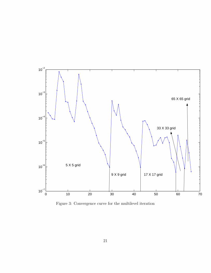
Our first experiment we run the model problem in 2D where L = −∇2 whichDrichlet boundary conditions, on a 652 grid points and use the LBFGS(10)method. We shoot for a total mass of 1.154. To obtain an eigenvalue withat least three digit accuracy we set (after some experiments) the number offixed point iterations to 7. We then solve the problem first on the single finegrid without any continuation and follow the iteration. To solve the problem

13

Grid Iterations Final mass52 29 1.360192 14 1.2592172 16 1.1584332 4 1.1538652 3 1.1539

Table 1: Iterations per grid for maximizing λ

on a single fine grid, we needed 44 fine grid iterations to reduce the absolutevalue of the gradient to 10−6. This number is better than the iteration countsreported in [15] in a factor of 3− 4 but as we see next, we can be much moreambitions then that. Recall that each iteration requires 14 solutions of thePoison equation thus even in 2D using multigrid methods, the problem iscomputationally expensive.

When we use a multilevel continuation technique we can do much better.First, initializing the first eigenvector with the coarse grid interpolation, wecan reduce the number of inverse iterations to 2 keeping the same accuracyand reducing nonlinearity. The number of iterations and the total mass oneach grid is summarized in Table 1.

As we can see, the number of the iterations on the coarsest grid is some-what large but this iteration is very cheap. Using the coarse grid solutionas an initial guess, the number of finer grid iteration reduces dramatically.Finally the number of the finest grid iteration is reduced to only 3. Sincewe solve only 4 Poison equations at each iteration (due to the good initialapproximation to the first eigenvector), compared with 14 when we do notuse multilevel methods, the cost of each fine grid iteration in the multilevelsetting is roughly 3.5 times cheaper than the iteration on a single grid. Thusthe overall saving is more then a factor of a hundred.

In this case, even though the number of iterations on the coarse grid waslarge, the line search did not fail and we did not need to use the continuationin the fixed point iteration. However, when starting from different startingmodels we have used this continuation on the coarse grid if the line searchfails.

The final result of the density on each grid in these experiments areplotted in Figure 1. The level-set function is plotted in Figures 2 Finally, weplot the convergence curve of this process in Figure 3. We can see that using

14

Grid Iterations Final mass52 38 1.60392 19 1.588172 12 1.567332 6 1.562652 4 1.562

Table 2: Iterations per grid for minimizing λ

the multilevel process, the initial iteration on the finest grid had roughly agradient norm of 10−5.

We repeat the experiment but this time we minimize λ by changing thesign in Equation (4). The results in this case are recorded in Table 2. Wesee that we keep the overall efficiency and that our formulation is insensitiveto this change.

7.2 Maximizing λ on a complicated domain

In the next experiment we demonstrate the ability of the level-set to changetopology. We solve the problem on a square domain with two holes with abutterfly shape. Drichlet boundary conditions are imposed inside and out-side. In this case we do not use a multilevel scheme as we are interested infollowing the changes in the density through the iteration.

We set the grid to 65 × 65 We set the total mass to 1.33 and tracethe iteration. The stopping criteria is set to when the absolute value ofthe gradient is smaller than 10−6. We start our iteration with a connectedshape. We see that the shape quickly disconnect into two separate shapesthat “travel” to the right place.

In this case there is no analytic solution to compare our results with.However, starting from different starting models yield identical results. Theresults are plotted in Figure 4.

7.3 Maximizing λ in 3D

As a third experiment we solve the same problem in 3D on a simple domain.The finest grid is set to 653 thus the size of the matrix is 2746252. We setthe total mass in this case to 1.11. Evaluating eigenvalues and eigenvectors

15

Grid Iterations Final mass52 52 1.26192 13 1.132172 9 1.116332 5 1.110652 2 1.112

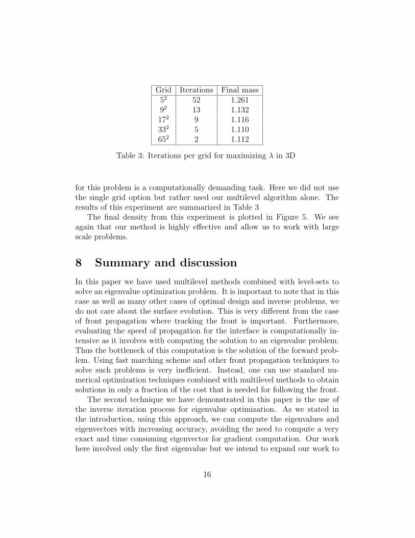
Table 3: Iterations per grid for maximizing λ in 3D

for this problem is a computationally demanding task. Here we did not usethe single grid option but rather used our multilevel algorithm alone. Theresults of this experiment are summarized in Table 3

The final density from this experiment is plotted in Figure 5. We seeagain that our method is highly effective and allow us to work with largescale problems.

8 Summary and discussion

In this paper we have used multilevel methods combined with level-sets tosolve an eigenvalue optimization problem. It is important to note that in thiscase as well as many other cases of optimal design and inverse problems, wedo not care about the surface evolution. This is very different from the caseof front propagation where tracking the front is important. Furthermore,evaluating the speed of propagation for the interface is computationally in-tensive as it involves with computing the solution to an eigenvalue problem.Thus the bottleneck of this computation is the solution of the forward prob-lem. Using fast marching scheme and other front propagation techniques tosolve such problems is very inefficient. Instead, one can use standard nu-merical optimization techniques combined with multilevel methods to obtainsolutions in only a fraction of the cost that is needed for following the front.

The second technique we have demonstrated in this paper is the use ofthe inverse iteration process for eigenvalue optimization. As we stated inthe introduction, using this approach, we can compute the eigenvalues andeigenvectors with increasing accuracy, avoiding the need to compute a veryexact and time consuming eigenvector for gradient computation. Our workhere involved only the first eigenvalue but we intend to expand our work to

16

the case of minimizing the gap between eigenvalues as well as other eigenvalueproblems.

Acknowledgment

The author would like to thank Stanley Osher for introducing the prob-lem.

References

[1] U. Ascher and E. Haber. Grid refinement and scaling for distributedparameter estimation problems. Inverse Problems, 17:571–590, 2001.

[2] U. Ascher and E. Haber. A multigrid method for distributed parameterestimation problems. Preprint, 2001.

[3] M. Bendsoe and C. Mota Soares. Topology design of structuts. KluwerAcademic, Dordrecht, MA, 1993.

[4] S. Cox and D. Dobson. Band structure optimization of two dimen-sional photonic crystals in h-polarization. J. Comput. Phys., 158:214–223, 2000.

[5] J. E. Dennis and R. B. Schnabel. Numerical Methods for UnconstrainedOptimization and Nonlinear Equations. SIAM, Philadelphia, 1996.

[6] H.W. Engl, M. Hanke, and A. Neubauer. Regularization of InverseProblems. Kluwer, 1996.

[7] C. Farquharson and D. Oldenburg. Non-linear inversion using generalmeasures of data misfit and model structure. Geophysics J., 134:213–227, 1998.

[8] E. Haber and U. Ascher. Preconditioned all-at-one methods for large,sparse parameter estimation problems. Inverse Problems, 2001. Toappear.

[9] E. Haber, U. Ascher, and D. Oldenburg. On optimization techniquesfor solving nonlinear inverse problems. Inverse problems, 16:1263–1280,2000.

17

[10] A Leito and O. Scherzer. On the relation between constraint regulariza-tion, level sets, and shape optimization. Inverse Problems, 19 (1):1–11,2003.

[11] A.S. Lewis. The mathematics of eigenvalue optimization. MathematicalProgramming, to appear, 2003.

[12] A.S. Lewis and M.L. Overton. Eigenvalue optimization. Acta Numerica,5:149–190, 1996.

[13] K. Neymeyr. Solving mesh eigenproblems with multigrid efficiency, inNumerical Methods for Scientific Computing. Variational problems andapplications. CIMNE, Barcelona, 2003.

[14] J. Nocedal and S. Wright. Numerical Optimization. New York: Springer,1999.

[15] S. Osher and F. Santosa. Level set methods for optimization problemsinvolving geometry and constraints i. frequencies of a two density inho-mogeneous drum. JCP, 171:272–288, 2001.

[16] M. Overton. On minimizing the maximum eigenvalue of a symmetricmatrix. SIAM J. on Matrix Analysis and Applications, 9(2):256–268,1988.

[17] M.L. Overton. Large-scale optimization of eigenvalues. SIAM J. Opti-mization, 2:88–120, 1992.

[18] A. Shapiro and M.K.H. Fan. On eigenvalue optimization. SIAM J. onOptimization, 5:552–569, 1995.

[19] U. Trottenberg, C. Oosterlee, and A. Schuller. Multigrid. AcademicPress, 2001.

18

1.2

1.4

1.6

1.8

0 0.5 1

0

0.5

11.2

1.4

1.6

1.8

0 0.5 1

0

0.5

1

1.2

1.4

1.6

1.8

0 0.5 1

0

0.5

11.2

1.4

1.6

1.8

17 X 17 Grid

0 0.5 1

0

0.5

1

1.2

1.4

1.6

1.8

33 X 33 Grid

0 0.5 1

0

0.5

1

1.2

1.4

1.6

1.8

Initial guess 5 X 5 Grid

9 X 9 Grid

65 X 65 Grid

0 0.5 1

0

0.5

1

Figure 1: Evolution of the density when using the multilevel approach

19

−0.4

−0.3

−0.2

−0.1

0

0.1

0.2

0.3

0 0.1 0.2 0.3 0.4 0.5 0.6 0.7 0.8 0.9 10

0.1

0.2

0.3

0.4

0.5

0.6

0.7

0.8

0.9

1

Figure 2: The final level set function on the finest grid

20

0 10 20 30 40 50 60 7010

−7

10−6

10−5

10−4

10−3

10−2

5 X 5 grid

9 X 9 grid 17 X 17 grid

33 X 33 grid

65 X 65 grid

Figure 3: Convergence curve for the multilevel iteration

21

Initial guess 5 Iter 10 Iter

15 Iter 20 Iter 25 Iter

34 Iter

Figure 4: Density distributions with the iteration

22

Figure 5: The final density on the finest 3D grid

23