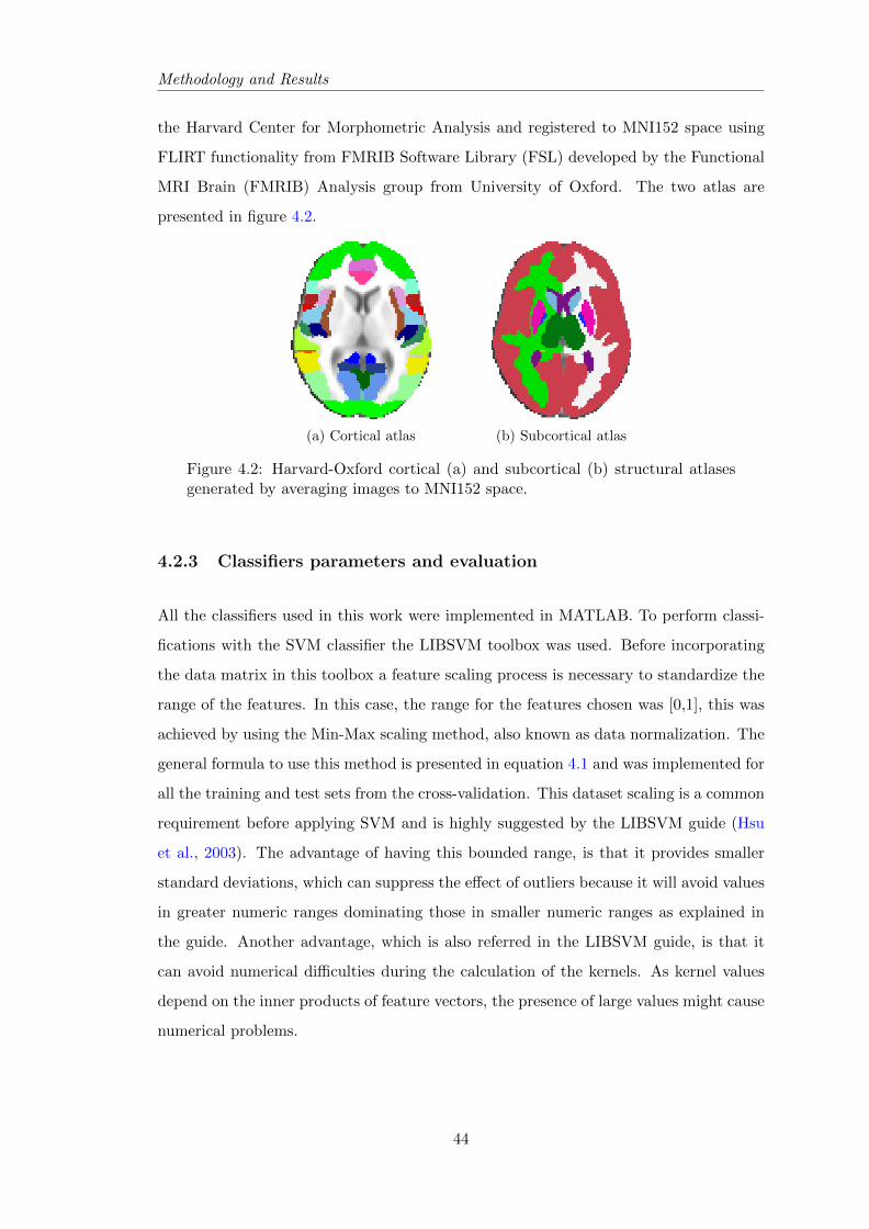
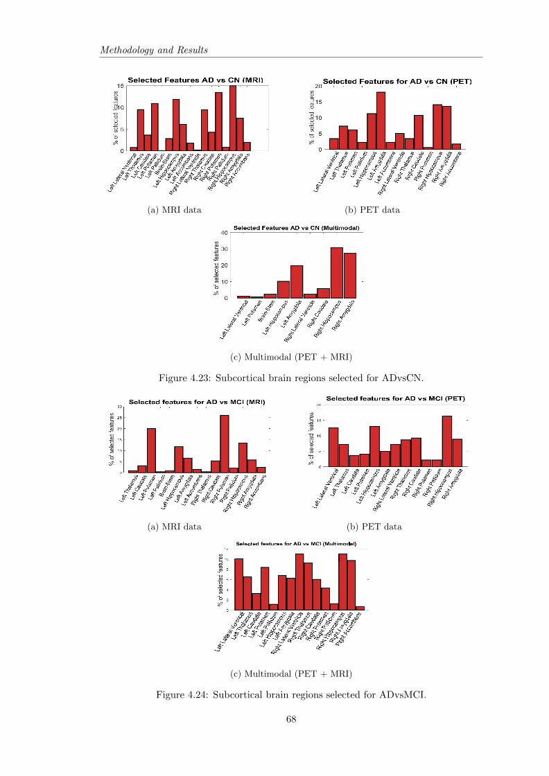
UNIVERSIDADE DE LISBOA FACULDADE DE CI ˆ ENCIAS DEPARTAMENTO DE F ´ ISICA A multimodal approach to distinguish MCI-C from MCI-NC subjects Rochelle Ann Costa Silva Mestrado Integrado em Engenharia Biom´ edica e Biof´ ısica Perfil em Sinais e Imagens M´ edicas Disserta¸c˜ ao orientada por: Orientador Externo: Professora Dra. Margarida Silveira, Instituto de Sistemas e Rob´ otica (ISR), Instiuto Superior T´ ecnico (IST) Orientador Interno: Professor Dr. Nuno Matela, Instituto de Biof´ ısica e Engenharia Biom´ edica (IBEB), Faculdade de Ciˆ encias da Universidade de Lisboa (FCUL) 2016
Transcript
UNIVERSIDADE DE LISBOA
FACULDADE DE CIENCIAS
DEPARTAMENTO DE FISICA
A multimodal approach to distinguish
MCI-C from MCI-NC subjects
Rochelle Ann Costa Silva
Mestrado Integrado em Engenharia Biomedica e Biofısica
Perfil em Sinais e Imagens Medicas
Dissertacao orientada por:
Orientador Externo: Professora Dra. Margarida Silveira, Instituto de Sistemas e
Robotica (ISR), Instiuto Superior Tecnico (IST)
Orientador Interno: Professor Dr. Nuno Matela, Instituto de Biofısica e
Engenharia Biomedica (IBEB), Faculdade de Ciencias da Universidade de Lisboa
(FCUL)
2016
’ Nobody ever figures out what life is all about, and it doesn’t matter. Explore the world.
Nearly everything is really interesting if you go into it deeply enough.’
- Richard Feynman
Acknowledgements
First of all, I would like to express my very special thanks to Prof. Dr. Margarida
Silveira, from Instituto Superior Tecnico (IST), for having accepted to be my supervisor
for this thesis in Institute for Systems and Robotics (ISR), in Lisbon. I am very grateful
for having had the opportunity and privilege to learn and achieve success in one of the
most important experience of my academic life. I truly value all her guidance, support,
patience in helping to solve the technical problems that occurred, and the knowledge
transmitted throughout the development of the present thesis. I also acknowledge all
the corrections and comments on this written work, which were fundamental.
I would also like to express my deep gratitude to Dr. Jonathan Young from Centre
for Neuroimaging Sciences, King’s College London, for responding very promptly to my
e-mails and clearly explaining the key steps to implement the method from his article.
I also thank Prof. Dr. Nuno Matela, for having promptly accepted to be my internal
supervisor, for being accessible to help me when needed, and for the comments and
suggestions on this written work.
My gratitude also goes to Prof. Dr. Eduardo Ducla Soares for presenting the wonderful
world of Biomedical Engineering in my 12th grade and to Dr. Maria Joao Rosa and Dr.
Janaina Mourao Miranda with whom I did an internship in London in my third year of
the course. They were instrumental in my choice of specialising in such an interesting
area which is Machine Learning.
I appreciate all the support and advice provided by my friends, which helped me over-
come stressful moments, and thank them for the great memorable times spent together,
during these 5 years of my academic life.
Finally, to my beloved parents I thank their love, trust, patience and motivation. A
special thank you to my brother Ryan, who has always been there for me at all times.
iv
Abstract
Alzheimer’s Disease (AD) is one of the most common neurodegenerative diseases, affect-
ing 60-80% from all dementia cases. Unfortunately, the cure for AD is still not known
and only some treatments can be done in its early stages to slow up the symptoms and
cognitive decline, avoiding worst patients’ living conditions. As most of the AD diagnoses
are late, it increases the difficulty of applying the strategies and treatments available.
Therefore, current studies aim at detecting AD at an early stage. For this purpose, they
are studying mild cognitive impairment (MCI) subjects, as this is normally the first
condition before developing AD. Nonetheless, not all MCI patients convert to AD, some
remain stable or even may reverse the cognitive decline. In this sense, being able to dis-
tinguish between MCI-converters (MCI-C) and MCI-non converters (MCI-NC) reveals
a quite important task.
In order to distinguish between these and other groups of subjects many classifiers can
be used. Classifiers are machine learning algorithms which apply artificial intelligence.
These are extremely useful to identify patterns in, for example, medical brain images,
to find disease related patterns and try to achieve an early and reliable diagnosis. The
Support Vector Machine (SVM) is a widely used classifier for AD studies and is very
appealing as it deals well with high-dimensional problems, which is present when using
neuroimages because of the high number of voxels in each image. Nonetheless, SVM is
a non-probabilistic classifier and only provides the class predicted for a given test. In
a clinical perspective, it would be advantageous to also have a confidence level about
the prediction made, to avoid diagnosis being hampered by overconfidence. Hence, of
late the interest in probabilistic classifiers is rising. The Logistic Regression (LR) and
the Gaussian Process (GP) are examples of probabilistic classifiers, but few studies used
these methods to present results for AD classification, additionally the analysis of the
posterior probability given by these classifiers is also still not well explored.
In this context, this thesis proposes the comparison of the performance of probabilistic
(LR and GP) and non-probabilistic (SVM) classifiers for AD context with special in-
terest in reaching good results for MCI-C vs MCI-NC. These tests were done using two
neuroimaging modalities: the deoxyglucose Positron Emission Tomography (FDG-PET)
and structural Magnetic Resonance Imaging (sMRI), in single modal and multimodal
approach. A whole-brain approach was chosen, to avoid restringing the model just for
certain brain regions. For feature selection methods, the LASSO and group LASSO with
L1/L2 regularization, for both single and multimodality cases, were used respectively.
Four different binary classification tests involving AD, MCI and elderly cognitive normal
(CN) subjects from the Alzheimer’s Disease Neuroimaging Initiative (ADNI) database,
vi
vii
were performed: AD vs CN, AD vs MCI, CN vs MCI and MCI-C vs MCI-NC with a con-
version period of 24 months. The results demonstrated the advantage of using GP and
LR as they can achieve state-of-the art classification results and be better than SVM, in
most cases, while providing posterior probabilities that will help evaluate how confident
the classifier is on its predictions. However, to distinguish MCI-C and MCI-NC, SVM
seemed to get better results, with LR being just a little worse than SVM. The poste-
rior probabilities from GP attracted more attention, because they demonstrated higher
confidence in results, whereas LR posterior probabilities were mostly near the thresh-
old value, meaning that the class is not chosen with a lot of confidence. Although the
multimodal approach did not show always the best results, for the MCI-C vs MCI-NC
classification it outperformed the single modality results, independently of the classifier
used. Thus, exhibits that is useful to joint information of different modalities to help
LASSO Least Absolute Shrinkage and Selection Operator
LIBSVM Library for Support Vector Machines
LONI Laboratory of Neuro Imaging
LR Logistic Regression
MCI Mild Cognitive Impairment
xvi
Acronyms xvii
MMSE Mini-Mental Status Exam
MNI Montreal Neurological Institute
MRI Magnetic Resonance Imaging
NIA National Institute on Aging
NINCDS-ADRDA National Institute of Neurological and Communicative Disorders
and Stroke-Alzheimer’s Disease and Related Disorders Association
PAD Pre-dementia Alzheimer Disease
PIB Pittsburgh Compound B
ROI Region Of Interest
SLEP Sparse Learning with Efficient Projections
SPM Statistical Parametric Mapping
SVM Support Vector Machine
TN True Negatives
TP True Positives
WM White Matter
WHO World Health Organization
Symbols
Greek Symbols
α Lagrange multiplier
λ Regularization parameter
λmax Maximum regularization parameter defined by SLEP toolbox
θ Hyperparameter
θMRI Hyperparameter which defines the weight for MRI data
θPET Hyperparameter which defines the weight for PET data
ξn Slack variable
Roman Symbols
K Kernel matrix
W Feature weight matrix
w Feature weight vector
X Feature data matrix
x Feature data vector
XMRI Feature matrix for MRI data
XPET Feature matrix for PET data
b Bias term
C SVM parameter
xviii
Symbols xix
D Data set
d Number of features
L Lagrangian
n Number of samples/subjects
s Weight for a given sample
t Number of tasks/modalities
y Sample label, (positive +1, or negative -1)
Chapter 1
Introduction
Alzheimer’s Disease (AD) is one of the most common neurodegenerative disorders in
older people, accounting for 60-80% of age-related dementia cases (Ye et al., 2011). The
disease causes neurons progressive damage or destruction and loss of their connections
in the brain, consequently the patient begins losing memory, thinking and behavior
abilities and reaches a state that they are entirely unable to take care of themselves,
having difficulties controlling even the most basic necessities and consequently, require
around-the-clock care. Most often, AD is diagnosed in people over 65 years of age (late-
onset), however some individuals younger than age 65 (early-onset) can also develop
the disease, but the risk of getting this disease is much higher as people get older.
Unfortunately, as neurons normally are not able to regenerate and do not undergo cell
division, all the caused damage in the brain cannot be recovered. Therefore, till date AD
is considered an irreversible brain disease which leads ultimately to death, because there
is currently no known cure and present treatments cannot stop AD from progressing,
they only can slow down the worsening of symptoms. The speed of progression can vary,
but an average point for survival time ranges from 3.3 to 11.7 years, with most cases in
the 7 to 10-year period (Todd et al., 2013).
Brookmeyer in 2007 reported that there were 26.6 million cases of AD in the world in
2006 and in 2050 one person in 85 will suffer from AD (1.2% of total population) or
106.8 million (Cornutiu, 2015). In Portugal the numbers from 2012 indicate that more
than 182 000 people suffer with dementia (this represents 1.71% of the population, a
little higher than the European mean which is 1.55%) (Alzheimer Europe, 2013). A
1
Introduction
report estimates from (World Health Organization (WHO) and Alzheimer’s Disease
International, 2012) point that the numbers from 2012 will double until 2030, and more
than triple by 2050. As most of the AD diagnoses are late, it increases the difficulty of
applying some strategies which are used actually to try reducing the progression of the
disease. For this reason and due to its big emotional and financial impact on society, AD
is a quite concerning public health issue and has been identified as a research priority
(Ballard et al., 2011).
Patients suffering from AD at a prodromal stage, i.e. when early symptoms appear and
might indicate the start of the disease before the characteristic symptoms occur, are,
mostly, clinically classified as amnestic mild cognitive impairment (aMCI). When refer-
ring to a patient with MCI it means that the patient has an early loss of brain function
before meeting criteria for the diagnosis of dementia. In most cases, the function lost is
memory, thus, commonly it can be named as aMCI. These patients show cognitive de-
cline greater than expected for their age and education level, however these alterations
are not severe enough to interfere with everyday activities (Alzheimer’s Association,
2016). According to (Petersen et al., 2010) study, they suggested that about 16% of
elderly people with no dementia are affected by MCI and that approximately two-thirds
of those with MCI have aMCI. Studies have also compared the rate of conversion of
MCI, they have shown that MCI patients convert to AD at an annual rate of 10-15%
per year compared with healthy controls who develop dementia at a rate of 1–2% per
year (Bischkopf et al., 2002). So, older MCI patients are at a greater risk of developing
AD. The patients that do indeed convert to AD are named as MCI-converters (MCI-
C). However, not all MCI patients will develop AD, some either develop other forms of
dementia (Vascular dementia; Dementia with Lewy bodies; Parkinson’s disease; Hunt-
ington’s disease), remain stable, or in a small minority, revert the process and go back
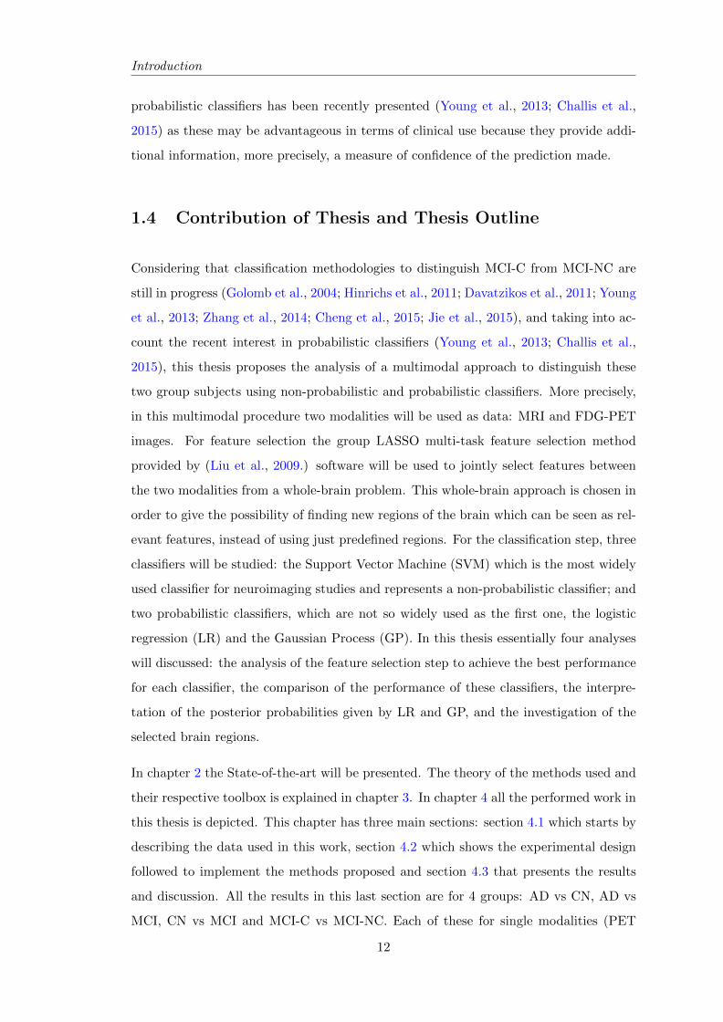
to normal cognition, so these are seen as MCI-non converters (MCI-NC), figure 1.1 de-
scribes this division. It is unclear why some MCI patients develop AD or other dementia
and others do not (Alzheimer’s Association, 2016).
1.1 Alzheimer’s Disease
AD is named after the German physician Dr. Alois Alzheimer, who first described this
disease in 1906 (Hippius and Neundorfer, 2003). He detected a dramatic shrinkage of the
2
Introduction
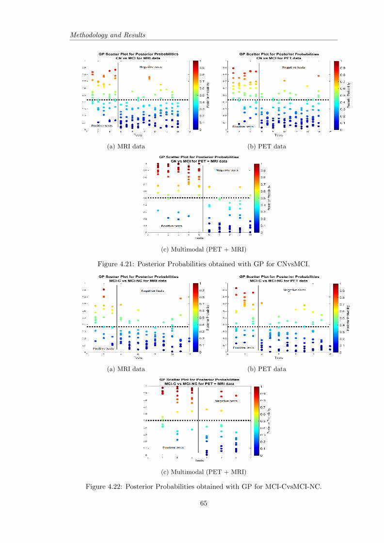
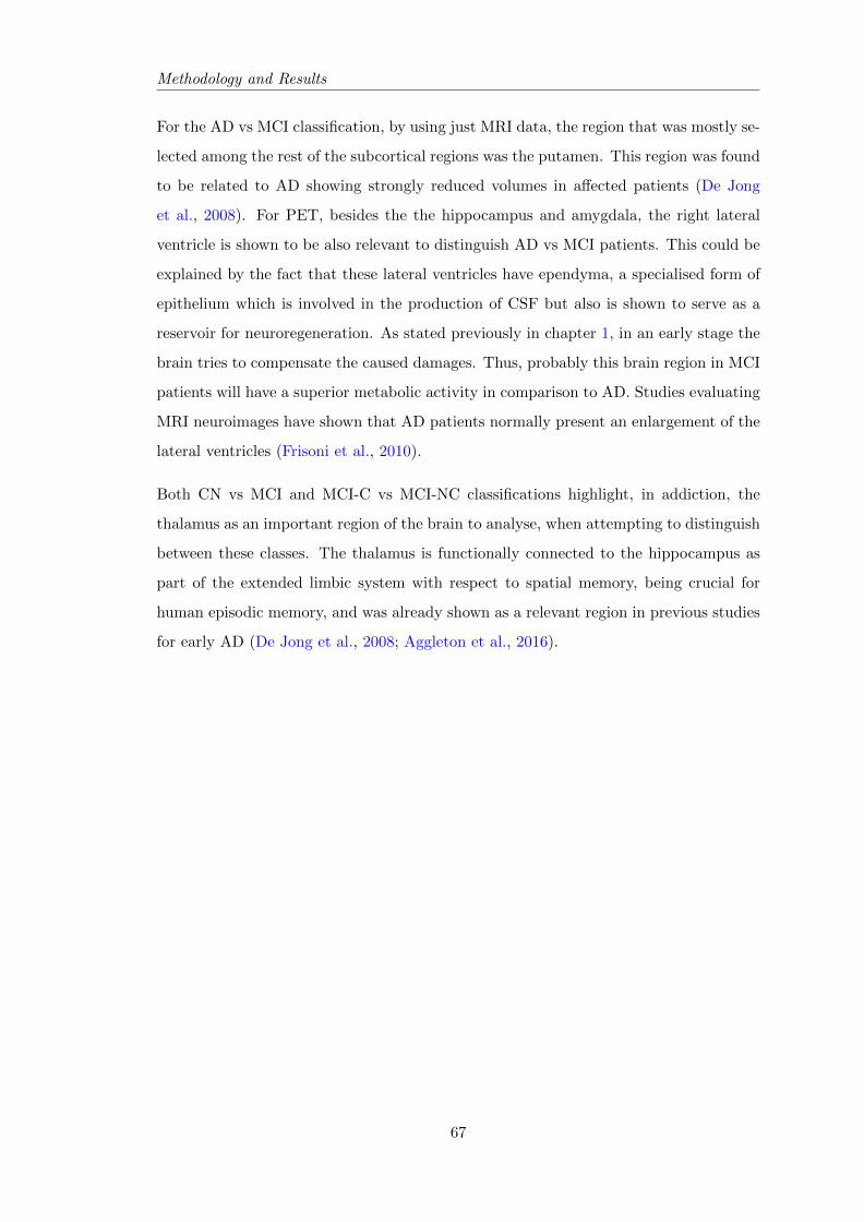
Figure 1.1: A conceptual model of possible developments after reaching MCIstate. They can convert to AD (MCI-C) or not (MCI-NC). Adapted from(Golomb et al., 2004)
brain and abnormal deposits in and around nerve cells when analysing the autopsy of
a patient who had profound memory loss and many psychological changes. Since then,
scientist have been investigating how AD affects the brain, trying to understand its real
cause and also several efforts to know how it can be treated are being made, but still
with little or no success.
In a healthy adult brain there are around 100 billion nerve cells (neurons), which are the
core structural and functional components of the brain and the nervous system. Typ-
ically the structure of a neuron consists of dendrites which receive the neural signal, a
cell body that will process the signal and an axon which will pass the signal electrically
through the neuron and when the electrical signal reaches the end of the axon this causes
the terminal branches to release chemical messengers called neurotransmitters. There-
fore, the neural communication actually involves an electrochemical communication. An
example of a neuron is presented in figure 1.2. In turn, these cells can connect to each
other by spaces called synapses, which count for approximately 100 trillion (Alzheimer’s
Association, 2016). The neurotransmitters travel across these synaptic clefts and bind
to the receptors present in the dendrites from neighbour neuron’s. This transmission
will cause the other neuron to become electrically active and the same process continues
and passes through other neurons.
3
Introduction
Figure 1.2: Structure of a neuron and how the nerve impulse travels.(http://www.appsychology.com/Book/Biological/neuroscience.htm)
The exact cause of AD is still to be fully understood. However, based on several research
done for AD along these years, two pathological hallmarks are known: the accumulation
of plaques of the protein beta-amyloid (Aβ) outside neurons and the formation of an
abnormal form of the protein tau (neurofibrillary tangles) inside the neurons (Ballard
et al., 2011). See figure 1.3 for illustration.
Figure 1.3: Illustration of the two pathological hallmarks in AD: formation ofamyloid plaques betwen neurons and neurofibrillary tangles inside the neurons.(http://www.brightfocus.org/alzheimers/)
The first hypothesis about the amyloid plaques suggested that the total amyloid load had
a toxic effect on neurons and consequently lead to neurons failure. With more studies
in this area, the pathological changes were more deeply investigated, more precisely the
4
Introduction
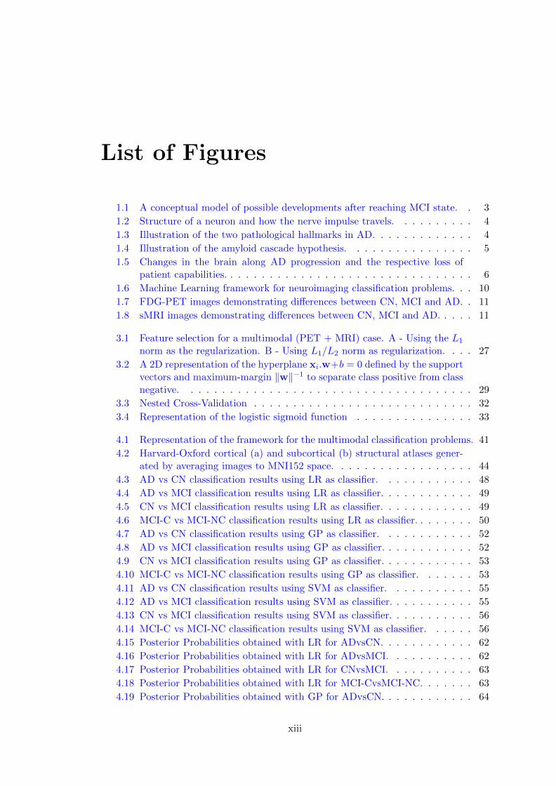
(Aβ) processing, and a more detailed hypothesis was formulated: the amyloid cascade
hypothesis. According to this hypothesis, the protein (Aβ) results from the cleavage
of the amyloid precursor protein (APP) and accumulates inside neuronal cells but also
extracellulaly where it aggregates into plaques and is believed to interfere with the
neurons communication by causing synaptic dysfunction and neuronal death (figure
1.4).
Figure 1.4: Illustration of the amyloid cascade hypothesis. Illustration from(Ballard et al., 2011).
The tau tangles are believed to unable the transport of nutrients and other essential
molecules inside neurons contributing therefore for their death.
These processes and changes in the brain are progressive. The first changes can oc-
cur without the patient feeling it (clinically silent), as the brain tries to compensate
the caused damages (Alzheimer’s Association, 2016). However, as the process starts
evolving, the brain can no longer compensate the damages and the first symptoms start
appearing in accordance to the brain regions affected. A scheme of the affected areas
along AD progress and the symptoms are presented in figure 1.5.
The first areas affected are normally in the medial temporal lobe from the brain cortex,
which suffers a shrinkage. More specifically the hippocampus is quite affected. As this
part of the brain plays a key role in formation of new memories, patients start having
difficulties in storing short-term memories. As years pass more neurons are affected from
other brain areas like lateral temporal and parietal temporal lobes; consequently the
patient begins suffering some difficulties in other activities like reading and recognising
objects. The disease spreads also to the frontal lobe. The frontal lobe is responsible for
executive functions such as planning, judgment, decision-making skills, and attention.
5
Introduction
Figure 1.5: Changes in the brain along AD progression and the respective loss ofpatient capabilities. (http://my-dementia.co.uk/Stages%20and%20Cases.html)
Consequently, in this phase, all these functions can decrease drastically. In a more severe
stage the disease reaches the occipital lobe and difficulties in seeing clearly rise.
The diagnosis of AD, at present, can only be done with certainty in autopsy by perform-
ing a histopathological confirmation, which involves a microscopic examination of brain
tissue. Thus, clinically, only probable diagnosis is possible. In addition, as this disease is
quite complex and not fully understood, a single medical test will not be sufficient. The
diagnosis has to be carefully evaluated by a physician, normally along with a neurologist
help, by following some established guidelines. In this context, the physician can require
many different tests and patients’ family help, in particular, as explained in (Alzheimer’s
Association, 2016), these include: 1- Obtaining medical background (including psychi-
atric and cognitive history) and family history from the patient; 2- Requesting a family
member or an person close to the patient to describe the changes in thinking skills and
behavior; 3- Executing cognitive tests and physical and neurologic examinations; and 4-
Acquiring patients’ blood tests and brain images.
1.2 Motivation and problem identification
There is a strong belief that pathological manifestations of AD may appear around
20 or more years before subjects become symptomatic (Alzheimer’s Association, 2016).
Therefore, it is important to find a way to diagnose even before the classical symptoms
6
Introduction
appear. An early and accurate diagnosis will allow patients to benefit from new treat-
ments or strategies that may delay the progress of the disease. In this sense, the aim of
today’s investigations in this area, is mainly to find the best possible methods which will
distinguish between MCI-C and MCI-NC, in order to know which patients will develop
AD and need treatment in a near future (i.e. within a few years), and target the disease
before irreversible damage or mental decline has occurred.
However, unfortunately the task of predicting conversion from MCI to AD is still known
to be difficult and presents challenges beyond that of classifying AD and cognitive normal
(CN) subjects or even that of classifying AD/CN vs MCI subjects. For that reason many
studies have achieved good results distinguishing AD from CN or CN from MCI, but
studies which analyzed MCI-C vs MCI-NC still have low classification performances.
This difficulty may be due to the “lag” between brain atrophy and cognitive decline
(Hinrichs et al., 2011).
From a public health perspective, treatments as well as clinical trials of therapeutics are
classified in terms of primary, secondary, and tertiary prevention interventions (Cavedo
et al., 2014). Primary prevention aims at reducing the incidence of illness across the
broad population by treating the subjects before disease appears, in other words, it tries
to eliminate the potential causes of the disease. Secondary prevention aims at preventing
disease at preclinical phases of illness. While tertiary prevention is focused on treating
the disease when it has been clinically diagnosed. In AD context, is seems obvious that
the primary and the secondary preventions are the ones which concern the population
because there is still no known cure for AD, and so tertiary prevention interventions
are still not very useful. In case of AD, when referring to a primary prevention it
means distinguishing between healthy and MCI patients, when referring to a secondary
prevention would be referring to detecting MCI subjects which will convert to AD.
1.3 Use of machine learning for early diagnosis
Machine learning is a subfield of computer science which uses algorithms of artificial
intelligence to perform pattern recognition, i.e., to identify patterns and regularities in
the data in order to build a model that will make accurate predictions on new data.
7
Introduction
Recent advances in neuroimaging techniques and image analysis have significantly con-
tributed to better understand the factors which change the brain and are associated
with Alzheimer’s disease. Combining them with machine learning algorithms will bring
enormous help in finding the best process to reach an early diagnosis of this disease.
This combination of elements of artificial intelligence and digital image processing gave
rise to a relatively young interdisciplinary technology called computer-aided diagnosis
(CAD). For this reason, CAD has gained increasing attention in the medical field in
order to simplify the task of interpreting test results by constructing a set of algorithms
and computational techniques which use pattern recognition to make future predictions
and correctly classify a certain patient.
To define a good classification model when using imaging data, five key steps need to be
followed: pre-processing of the data, feature extraction, feature selection, classification
and finally the evaluation of the performance of the classification results.
The first steps: pre-processing and feature extraction and feature selection are cru-
cial to perform when using neuroimaging data because without these most probably
good results for classification would be difficult to get. This is because medical images
can have noise and intensity-inhomogeneity, and in addition, when comparing different
scans they might not all be aligned so pre-processing will overcome these issues. The
pre-processing can include: motion correction with realignment, spatial normalization
and spatial smoothing. Furthermore, when dealing with CAD, there exists the high
dimensional problem of neuroimaging data, as neuroimages are characterized by having
high dimensionality, i.e. having a very large number of voxels in each image. Thus,
when analyzing pattern recognition for neuroimaging studies, the number of voxels is
much higher than the number of scans/subjects available. This leads to two big prob-
lems: it will require a large amount of memory and computation time and can lead to
overfitting, which means that it gives rise to a model that overfits the training sample
and generalizes poorly to new samples. One of the first steps to overcome this issue is
by performing feature extraction. This can be done by extracting, for example, some
predefined regions of interest (ROI) which can be meaningful for the study. A feature se-
lection on the extracted features can then be performed. Feature selection is the process
of selecting a subset of features that can be meaningful and relevant for the classifica-
tion procedure. The feature selection is quite crucial for various reasons: it simplifies the
model facilitating interpretation; it makes it computationally more effective as it requires
8
Introduction
shorter training times and it enhances generalization by reducing overfitting. Hence, an
effective feature selection could not only speed up computation, but also improve the
classification performance (Liu et al., 2014).
It is also very common to use kernel methods to solve the high dimensionality of image
data. Kernel methods consist of a collection of algorithms based on pair-wise similarity
measures between all examples (feature vectors), summarized in a kernel matrix that
will have n× n dimensions instead of data matrix dimensions n× d (n-number of sub-
jects/scans; d- number of voxels). Given two feature vectors, a kernel function returns
a real number characterizing their similarity. The simplest operation one can perform
to measure the similarity between two vectors is a dot product (linear kernel). So, in
pattern recognition the kernel matrix is many times used instead of the data matrix
to simplify the calculations when using neuroimages data, because it makes the model
computationally more efficient.
There are many types of machine learning algorithms like supervised learning, unsu-
pervised learning and semi-supervised. Unlike in unsupervised learning, in supervised
learning all the training data (i.e. the examples provided to the classifier) are properly
labeled by hand (i.e. all examples have their class). It consists in two important steps:
training and testing. During the training phase, the algorithm learns some mapping be-
tween patterns and the labels and then creates a function that can accurately predict the
labels for unseen new patterns. For AD classification problems, the method mostly used
is the supervised learning method. Nonetheless, semi-supervised learning algorithms are
also recently being tested. Furthermore, in supervised learning we can have two types
of pattern recognition: classification and regression. If one wants to distinguish classes
or subjects (e.g. distinguish MCI from AD) the learnt function is a classifier model and
the labels are discrete values, for example -1, 1 for negative class and positive class,
respectively. If instead, one wants to predict a specific value (e.g. values of cognitive
test scores), then the learnt function will be a regression model and the labels in this
case are continuous values.
The final step, after using the classification algorithm, is then to validate it by evaluating
its performance. This evaluation is done by performing a cross-validation and looking
into the statistics of the model. A good classification model, will present high accuracy
(test’s ability to correctly detect or exclude a condition correctly), high sensitivity (test’s
9
Introduction
ability to identify a condition correctly) and high specificity (test’s ability to exclude
a condition correctly) values. These statistical measurements are calculated by the
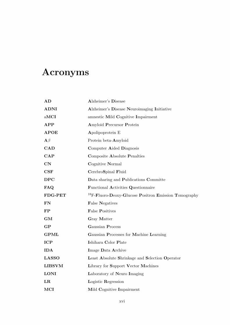
formulas presented in figure 1.6, where TP is the number of true positives, TN the
number of true negatives, FP the number of false positives and FN the false negatives.
This figure 1.6 presents the machine learning framework usually followed for classification
problems using neuroimaging data.
Figure 1.6: Representation of the framework for neuroimaging classificationproblems.
For AD classification studies, a wide range of different medical information could be used
as data to distinguish between patients with AD from those who do not have the disease,
or to determinate which are more likely to develop AD. These data, in a machine learning
context, are normally called modalities, and include: neuroimages, neuropsychological
tests, genetic tests, and cerebrospinal fluid (CSF) tests. The two most widely used
PET) that measures the cerebral metabolic rate for glucose, and structural Magnetic
Resonance Imaging (sMRI) which provides information about brain morphometry and
therefore can capture brain tissue atrophy related to the loss of neurons (Vemuri and
Jack, 2010). Furthermore, these could be used separately or together giving rise to a
multimodal classification approach. Existing studies have indicated that different modal-
ities can provide essential complementary information and therefore improve accuracy
in disease diagnosis, some of these studies will be presented in chapter 2. An illustration
of these two image modalities is presented in figures 1.7 and 1.8.
10
Introduction
Figure 1.7: Example of FGD-PET images from cognitive normal (left), MCI(middle) and AD (right) subjects. The color scale represents the magnitudeof 18F-FDG standardized uptake value ratio (SUVR) which is proportional toglucose uptake. By these images one can identify lower SUVRs in MCI and ADwhen compared to cognitive normal. Illustration from (Schilling et al., 2016).
Figure 1.8: Structural MRI images from an older cognitively normal (left),an amnestic mild cognitive impairment (middle) and an Alzheimer’s disease(right) subjects demonstrating progressive brain tissue atrophy. Illustrationfrom (Vemuri and Jack, 2010).
The feature selection for the neuroimage multimodal case can be performed indepen-
dently in each modality. However, this may overloook the complementary information
conveyed in different modalities. More recently, studies have used multi-task learning
to perform the feature selection for a multimodal approach, where each modality is seen
as a task. Multi-task learning is based on a procedure which takes a number of tasks
simultaneously and exploits the commonalities between them. So the objective is to
defect the intrinsic relationship among different tasks, which can lead to a better results
than when learning the tasks independently (Liu et al., 2014).
In terms of classifiers, these can also be distinguished by their property of providing a
probability. Most of the classification done in AD studies are based in non-probabilistic
classifiers (Zhang et al., 2011; Hinrichs et al., 2011; Liu et al., 2014; Jie et al., 2015),
which only provide the class that a sample should belong to. Nonetheless, interest in
11
Introduction
probabilistic classifiers has been recently presented (Young et al., 2013; Challis et al.,
2015) as these may be advantageous in terms of clinical use because they provide addi-
tional information, more precisely, a measure of confidence of the prediction made.
1.4 Contribution of Thesis and Thesis Outline
Considering that classification methodologies to distinguish MCI-C from MCI-NC are
still in progress (Golomb et al., 2004; Hinrichs et al., 2011; Davatzikos et al., 2011; Young
et al., 2013; Zhang et al., 2014; Cheng et al., 2015; Jie et al., 2015), and taking into ac-
count the recent interest in probabilistic classifiers (Young et al., 2013; Challis et al.,
2015), this thesis proposes the analysis of a multimodal approach to distinguish these
two group subjects using non-probabilistic and probabilistic classifiers. More precisely,
in this multimodal procedure two modalities will be used as data: MRI and FDG-PET
images. For feature selection the group LASSO multi-task feature selection method
provided by (Liu et al., 2009.) software will be used to jointly select features between
the two modalities from a whole-brain problem. This whole-brain approach is chosen in
order to give the possibility of finding new regions of the brain which can be seen as rel-
evant features, instead of using just predefined regions. For the classification step, three
classifiers will be studied: the Support Vector Machine (SVM) which is the most widely
used classifier for neuroimaging studies and represents a non-probabilistic classifier; and
two probabilistic classifiers, which are not so widely used as the first one, the logistic
regression (LR) and the Gaussian Process (GP). In this thesis essentially four analyses
will discussed: the analysis of the feature selection step to achieve the best performance
for each classifier, the comparison of the performance of these classifiers, the interpre-
tation of the posterior probabilities given by LR and GP, and the investigation of the
selected brain regions.
In chapter 2 the State-of-the-art will be presented. The theory of the methods used and
their respective toolbox is explained in chapter 3. In chapter 4 all the performed work in
this thesis is depicted. This chapter has three main sections: section 4.1 which starts by
describing the data used in this work, section 4.2 which shows the experimental design
followed to implement the methods proposed and section 4.3 that presents the results
and discussion. All the results in this last section are for 4 groups: AD vs CN, AD vs
MCI, CN vs MCI and MCI-C vs MCI-NC. Each of these for single modalities (PET
12
Introduction
and MRI) and for multimodality (PET + MRI). Finally, the conclusion and future work
suggestions are presented in chapter 5.
The innovation in this thesis is the comparison of the performance of non-probabilistic
and probabilistic classifiers in a whole-brain approach using LASSO with L1 regulariza-
tion and group LASSO with L1/L2 regularization as the feature selection methods, for
both single and multimodality respectively, and the analyses of the posterior probabili-
ties provided by LR and GP.
13
Chapter 2
State-of-the-art
The publication of the National Institute of Neurological and Communicative Disorders
and Stroke-Alzheimer’s Disease and Related Disorders Association (NINCDS-ADRDA)
criteria in 1984 represented a breakthrough in the diagnosis of AD (McKhann et al.,
1984). These criteria established that the clinical diagnosis should be based on certain
characteristics: medical history, clinical examination, neuropsychological testing, and
laboratory assessments. However, most demented patients were seen by community
physicians who often did not detect dementia or misdiagnosed it, and for pre-dementia
AD (PAD) detection this criteria did not show enough sensitivity (Alom et al., 2012). In
this context, researchers began developing studies which test machine learning methods
in order to understand if new guidelines could be suggested to facilitate physicians in the
diagnosis process. Presently, with the research done since then, these guidelines from
the 1984 criteria were updated with new guidelines established by the National Institute
on Aging (NIA) and the Alzheimer Association, in 2011 (Sperling et al., 2011; Albert
et al., 2011; McKhann et al., 2011; Jack et al., 2011). According to this criteria, the
brain changes due to Alzheimer’s begin several years (20 or more) before symptoms, and
suggest that, in some cases, MCI is an early stage of Alzheimer’s, whereas the earlier
criteria from 1984 would require the appearance of memory loss and cognitive decline in
order to make a diagnosis of AD. Although this new criteria for a preclinical phase of AD
is still not used by doctors for clinical diagnosis, it will help a lot for research purposes.
These new guidelines also added other tests that could facilitate an early diagnosis, like
for example the use of neuroimages.
14
State-of-the-art
One of the first studies using machine learning for AD diagnosis was (Shankle et al.,
1997). They used machine learning algorithms combined with clinical data such as
subjects demographic data (age, gender, education) and neuropathological tests, like
Functional Activities Questionnaire (FAQ), the Mini-Mental Status Exam (MMSE),
and the Ishihara Color Plate (ICP) tasks, to learn rule sets that would help detect very
early stages of dementia from normal aging and the results were as good as or better
than any rules derived from knowledge provided by expert clinicians. This demonstrated
the importance of exploiting machine learning techniques for AD early diagnosis.
Most machine learning studies in this area are making efforts to understand which
biomarkers are able to indicate early stages of AD. A biomarker is a biological factor
that can be measured to accurately and reliably indicate the presence or absence of
disease, or risk of developing a disease (Alzheimer’s Association, 2016). Examples being
studied for AD include beta-amyloid and tau levels in CSF, genetic risk factors and
brain changes detectable by brain imaging techniques. However, the difficulty rises as
these indicators may change at different stages of the disease process. In addition, for
a biomarker to be validated in order to be used as medical test for clinical diagnosis,
multiple studies in large groups of people have to be made and proven that it accurately
and reliably indicates the presence or absence of AD. These factors make it difficult to
validate biomarkers for AD and researchers are still investigating these promising candi-
dates. Although these candidates are not still seen as entirely validated biomarkers for
clinical use, they can provide comprehensive information about the disease being help-
ful to investigators in machine learning studies and also to physicians and neurologists,
specially the neuroimaging techniques, as they also allow the detection of brain changes
associated with AD. These techniques will be presented in the following paragraphs.
Structural Magnetic Resonance Imaging (sMRI) is an extremely important image modal-
ity for AD studies since it helps detecting brain atrophy as it was presented in previous
chapter in figure 1.8. In AD, brain atrophy occurs in a characteristic topographic distri-
bution, it begins in the medial temporal lobe and spreads to the lateral temporal areas,
and medial and lateral parietal areas (Cavedo et al., 2014). The most common sMRI
measure employed in AD is the atrophy of the hippocampus, recently recommended by
the revised criteria for AD as one of the core biomarkers (Albert et al., 2011; McKhann
et al., 2011; Jack et al., 2011). In this sense, several studies proposed classification
methods to discriminate between patients with AD or MCI and CN based on sMRI like
15
State-of-the-art
for example (Kloppel et al., 2008; Davatzikos et al., 2008). Comparing performance re-
sults of these studies an other sMRI studies may not be fully correct because they were
assessed on different populations. Many factors as: degree of impairment, age, gender,
genotype and level of education could be affecting the evaluation of the prediction accu-
racy. Therefore, in order to have the possibility to compare different performance results
(Cuingnet et al., 2011) studied 10 methods of classification of AD using sMRI with the
same population. Most of the methods showed high accuracy in classifying AD and CN,
nevertheless at the prodromal stage, i.e. for MCI, their sensitivity was very low. This
suggests the need of combination with other modalities, to overcome this difficulty.
Functional Magnetic Resonance Imaging (fMRI) has also been used for AD detection.
This modality tracks changes associated with blood flow, more precisely, it measures
the blood-oxygen-level dependent (BOLD) signal, reflecting the regional neuronal acti-
vation and intracortical processing. As a primary prevention biomarker, it still needs
considerable research and development work, because it has the issue of possible con-
found between normal aging and development of AD-related pathology. Normal aging
alters potential fMRI biomarker and alterations that are seen in MCI group are similar
to middle aged healthy controls (Cavedo et al., 2014). Therefore, at the moment, the
main use of fMRI would be in secondary prevention trials, which is actually the main
concern in this area. However, it should be noticed that pathologies other than AD,
such as Major Depression, can mimic the symptoms experienced by MCI patients, and
have also been shown to induce changes in functional connectivity (Challis et al., 2015).
So, further work needs to be done to better understand the relationship between BOLD
signal and clinical changes in dementia and non dementia cases.
As already referred in chapter 1 and presented in figure 1.7, another imaging modality
widely used for AD detection and study of its progression is 18F-fluorodeoxyglucose
(FDG) positron emission tomography (PET). FDG-PET is a functional marker that
measures tissue uptake of glucose and can therefore be linked to the detection of cortical
synaptic dysfunction. Normally it can reveal hypometabolism in the temporoparietal
regions, posterior cingulate cortex, and frontal lobe even prior to atrophy (Schilling et al.,
2016). This image modality has been approved in the USA for diagnostic purposes and
is sensitive and specific for AD detection in its early stages (Ballard et al., 2011) and
revealed to be a good predictor of MCI progression within the next 2 years combining
clinical covariates (Shaffer et al., 2013).
16
State-of-the-art
In recent years, researches have also studied a new modality called carbon 11-labeled
Pittsburgh Compound B (11C-PIB) PET. This modality provides both perfusion and
amyloid deposition information. Combining this modality with structural MRI good
results were achieved (Liu et al., 2015). However, this study was basically to distinguish
between AD vs CN (accuracy 100%) and MCI vs CN (accuracy 85%) and did not
explore MCI conversion to AD. The ones that indeed evaluated MCI conversion like the
longitudinal study from (Zhang et al., 2014) did not get such good results and showed
high sensitivity results (83-100%) but poor specificity (46-88%). This was explained
by the fact that positive results of PIB-PET were also present in other patients with
other diseases (Lewy body dementia, Parkinson) and also in some normal subjects. For
this reason, prior to 11C-PIB-PET being widely used as diagnostic modality it is still
important to demonstrate its accuracy, as it is a high cost investigation biomarker.
Furthermore, some AD studies were also based on cerebrospinal fluid (CSF) biomarkers.
At present there are three main CSF possible biomarkers for AD molecular pathology:
total tau protein (T-tau) that reflects the intensity of neuronal degeneration; hyperphos-
phorylated tau protein (P-tau) that probably reflects neurofibrillary tangle pathology;
and the 42 amino-acid-long form of amyloid beta (Aβ42) that is inversely correlated with
Aβ pathology in the brain (Cavedo et al., 2014). So, when using this modality for AD
prediction these are the ones which are used as CSF features, like it was done in (Cheng
et al., 2015).
In addition, genetic factors play an important role in late onset Alzheimer’s disease (Al-
bert et al., 2011). Variants of the apolipoprotein E (APOE) gene, found on chromosome
19, are known to affect the risk of developing AD. These are: APOE ε2, which is rel-
atively rare and may provide some protection against the disease; APOE ε3, which is
the most common allele, and is believed to play a neutral role in the disease (neither
decreasing nor increasing risk); and APOE ε4, which is the strongest known genetic risk
factor for AD and present in about 25% to 30% of the population and in about 40%
of all people with AD (Liu et al., 2013; Crenshaw et al., 2013). So people who develop
Alzheimer’s are more likely to have an APOE ε4 allele than people who do not develop
the disease.
Neuropsychological assessments have been used to grade the cognitive state of patients
(Folstein et al., 1975) and to characterize dementia associated with AD in several studies
17
State-of-the-art
(Shankle et al., 1997; Salmon and Bondi, 2009; Chapman et al., 2010; Weintraub et al.,
2012). A very common neuropsychological test is the MMSE already mentioned in this
chapter when referring to (Shankle et al., 1997) study, one of the first using machine
learning methods for AD diagnosis. The neuropsychological tests have proven to be
extremely useful to identify the cognitive profiles, determine patterns of impairment,
assess changes of impairment over time and also after treatment, and in fact, have been
widely used clinically to achieve a probable diagnosis of the disease (McKhann et al.,
2011). These are normally the preferred assessments used clinically because they present
some advantages and facilities like being inexpensive in comparison with other types of
exams, as neuroimaging, and are totally innocuous for the patients, compared to invasive
tests like nuclear medicine imaging.
Almost all of the data from these different modalities described above, used as predictors
for the disease, can be found in Alzheimer’s Disease Neuroimaging Initiative (ADNI)
data repository (http://adni.loni.usc.edu/data-samples/access-data/). All ADNI data
is archived in a secured and encrypted system through Image Data Archive (IDA), of
the University of Southern California’s Laboratory of Neuro Imaging (LONI), and can
be accessed with proper authorization provided by ADNI Data sharing and Publications
Committee (DPC). This well-curated scientific data repository is remarkably successful
across the globe, and has been a huge help for studies in this area providing data since
2004. According to (Murray, 2012) more than 1300 investigators have been granted
access to ADNI data, resulting in extensive download activity that exceeds 1 million
downloads of imaging, clinical, biomarker and genetic data. ADNI has data of AD,
MCI patients and elderly cognitive normal (CN). These participants are followed and
reassessed over time to track the pathology of the disease as it progresses.
2.1 Multimodality
Given that different modalities can help in the detection of different characteristics, an
approach combining more than one modality would be preferable. Multimodal neu-
roimaging, which is the combination of more than one image modality, may play an
important role with regard to early and reliable detection of subjects at risk of develop-
ing AD, for two important reasons. Firstly, neurodegeneration in AD cannot be reduced
to a singular pathological process in the brain (Cavedo et al., 2014). Thus, different
18
State-of-the-art
modalities can detect different important neuropathological aspects which can facilitate
the detection of the disease. Secondly, it is well accepted that the onset of appear-
ance of these different neuropathological aspects in the brain may occur subsequently
and not simultaneously (Cavedo et al., 2014). Therefore, depending on which stage the
disease is, one modality may detect a certain pathological characteristic better than
other. Intuitively, integration of more than one modality may uncover the previously
hidden information that cannot be found using just a single modality. In this context,
multimodality is seen as a very useful tool to achieve better classification performances
(Zhang et al., 2012; Cavedo et al., 2014; Uludag and Roebroeck, 2014). Several studies
have exploited the fusion of the multiple modalities to improve AD or MCI classification
performance. Some recent studies which use multimodality are presented in table 2.1.
It is possible to see how using different modalities allows better results. For example,
(Jie et al., 2015) tests two different multimodal cases MRI+PET and MRI+PET+CSF,
using the same population, and shows that the second presents better results. In com-
parison with single modality, the multimodal approach requires a more careful handling
of the data as in this case data from different modalities have to be joined and the num-
ber of features given to the classifier rises. The simplest way to combine the data, which
was done in many studies (Bouwman et al., 2007; Vemuri et al., 2009; Walhovd et al.,
2010) is by concatenating all the features of each modality in the same vector. Other
more powerful methods include allocating kernels for each modality and then using a
multi-kernel learning method to aggregate all kernels in one only kernel like it is done
in (Hinrichs et al., 2011; Zhang et al., 2011).
Study Subjects Modalities Classifier AD vs CN MCI vs CNMCI-C
vs MCI-NC
Zhang et al., 2011 51 AD + 99 MCI + 52CN MRI + PET SVM 90.6% — —Zhang et al., 2011 51 AD + 99 MCI + 52CN MRI + PET + CSF SVM 93.2% 76.4% —Hinrichs et al.,2011
48 AD + 66 CN MRI + PET SVM 87.6% — —
Hinrichs et al., 2011 48 AD + 66 CNMRI + PET + CSF+ APOE +Cognitive scores
SVM 92.4% — —
Huang et al., 2011 49 AD + 67 CN MRI+PET SVM 94.3% — —Zhang et al., 2012 45 AD + 91 MCI + 50CN MRI + PET + CSF SVM 93.2% 83.2% —Gray et al., 2013 37 AD+ 75 MCI+ 35 CN MRI+ PET+ CSF+ genetic RF 89.0% 74.6% 58.0%Liu et al., 2014 51 AD+ 99 MCI+ 52 CN MRI+ PET SVM 94.4% 78.8% 67.8%
Jie et al., 201551 AD+ 99 MCI+ 52CN
MRI+ PET SVM 95.0% 79.3% 68.9%
Jie et al., 201551 AD+ 99 MCI+ 52CN
MRI +PET+ CSF SVM 95.4% 83.0% 72.3%
Table 2.1: Accuracy of state-of-the-art Multimodality studies.
19
State-of-the-art
2.2 Feature Selection
As stated in the previous chapter, feature selection is a crucial step prior to any classi-
fication performed on high-dimensional data, because it reduces the number of features
given to the classifier, leading therefore to sparse representations of data. As stated in
(Yu, 2003), since 1970’s the problem of feature selection has been extensively studied
by the machine learning community and it has been proven that it can be effective to
remove irrelevant and redundant features.
For neuroimaging studies there are essentially two ways of dealing with feature selection
depending on the feature extraction chosen: 1- extracting specific brain regions, which
are called regions of interest (ROI) and then performing feature selection in these regions;
2- using feature selection methods to select only the important features of the whole-
brain. Many researchers opt for the first approach (Zhang et al., 2011; Zhu et al., 2015;
Lahmiri and Boukadoum, 2013; Young et al., 2013) to avoid the high dimensionality
problem. For example, in (Zhang et al., 2011) they select 93 ROIs and then average
intensity of each ROI region having in total just 93 features for each neuroimage modality,
in (Young et al., 2013) they choose to select 10 regions according to (Braak and Braak,
1995), therefore reducing drastically the computational time. However this approach can
have some issues. First if there are no ROI’s known a priori, and second having ROI’s a
priori will not give the possibility to find new important regions. On the one hand, it can
be logical and facilitating to use just ROI’s because they are based in previous studies
which have proven a certain theory driven assumptions of which areas are most involved
in the disease, nonetheless, research must be done not only to confirm findings but also
to expand them, specially for AD case, where absolute knowledge is still on construction.
Therefore, a whole-brain analysis may give new and interesting information, in addition
to the one already known. On the other side, choosing to design a whole-brain classifier
is quite challenging as it will present a lot more features. Typically the consequence
is an overfitting of the data, leading to high accuracies for data used in designing the
classifier, but poor classification accuracies for new independent test data. To overcome
this problem, there is a huge need to use of feature selection methods.
A well-known method is the Least Absolute Shrinkage and Selection Operator (LASSO)
method, introduced in 1996 (Tibshirani, 1996). This method uses a regularized L1-
penalty for sparse variable selection. The L1-norm regularization was already used for
20
State-of-the-art
regression problems in several studies, but also has become popular topic in the context
of classification problems. For the regression problems the most popular loss function
used is the least squares estimate (Schmidt, 2005), for classification problems, however,
least squares estimate may not be adequate, as it gives poor predictions compared to
other loss functions, like logistic regression (Rosasco et al., 2004). The comparison of
the L1 penalty and the L2 penalty was also performed, and results showed that models
produced with L1 penalty often outperformed the ones produced with L2. (Schmidt,
2005).
Further work have also extended the LASSO for multi-task problems by using other
regularization parameters, in particular the L1/Lq regularization, with 1≤ q ≤ ∞,
proposed by (Yuan and Lin, 2006) for regression and extended for classification in (Meier
et al., 2008). The L1/Lq regularization belongs to the composite absolute penalties
(CAP) family. When q=1, this extension is equivalent to the L1-penalty problem; when
q>1, the L1/Lq regularization promotes group sparsity in the resulting model, which
is quite desirable in many applications of classification problems. Studies analyzed also
the influence of different values for q. For example, the results of (Liu and Ye, 2010)
showed that smaller values of q had lower balanced error rates then higher values of q.
Another study also performed this analysis of the q values, in this case for a multi-task
learning with large scale experiments (Vogt and Roth, 2012), and the results also showed
better results for lower values of q more precisely for values between 1.5 and 2. Thus,
L1/L2 regularization seem to be the preferred choice to use for the model creation. This
L1/L2 norm penalty was already used for AD studies. In (Zhou et al., 2011) they used it
for regression, specifically they tested a multi-task regression problem predicting disease
progression measured by cognitive tests. This method of using LASSO with the L1/Lq
penalty for multi-task is also known as the the group LASSO multi-task method or just
group LASSO, for simplification.
2.3 Classifiers
Most of machine learning studies carried out for AD classification from neuroimaging
problems used the Support Vector Machine (SVM) algorithm as the classifier (Zhang
et al., 2011; Hinrichs et al., 2011; Liu et al., 2014; Jie et al., 2015), due to its good
accuracy, ability to cope with very high-dimensional data (several features and small
21
State-of-the-art
number of examples) as it uses kernels, and for providing a unic solution every time the
problem is solved with the same inputs and same conditions. In fact, all studies presented
in table 2.1 used SVM as the classifier, expect for (Gray et al., 2013) which used random
forest (RF). Although SVM can bring good results and has big advantages, this classifier
is a non-probabilistic binary classifier which uses a supervised learning algorithm, and
the use of other classifiers, like probabilistic classifiers, could also be helpful for these
kind of studies.
One example is Logistic Regression (LR) which is able to predict, given a sample input,
a probability distribution over a set of classes, rather than only outputting the most
likely class that the sample should belong to. So, it provides classification with a degree
of certainty. Nonetheless, it is worth noting that LR should not be used when there are
a large number of features in comparison to the number of training samples, because
of the problem of overfitting. In this sense, sparse models are necessarily needed for
neuroimaging pattern recognition studies, which is achieved by adding regularization
parameters as described above in section 2.2. In (Rao et al., 2011) they tested LR with
L1 and also another penalty, the L2, for classification of AD vs CN based on sMRI,
and presented classifications with better accuracies when using L1 than when using only
the L2 regularization. Furthermore, (Ryali et al., 2010) used LR with a combination of
L1 and L2 norm regularization for whole-brain classification of fMRI data, however not
for AD applications. With their work they could identify relevant discriminative brain
regions and accurately classify fMRI data.
StudySubjects
(MCI-NC; MCI-C)Modalities Conversion period Accuracy AUC
Nho et al., 2010 355 (205; 150) MRI + APOE+ family history 0-36 months 71.6% —Zhang et al., 2011 99 (56, 43) MRI + PET + CSF 0-18 months (sens 91.5% spec 73.4%) —Davatzikos et al.,2011
239 (170, 69) MRI + CSF 0-36 months 61.7% —
Hinrichs et al.,2011
119MRI + PET + CSF+APOE +Cognitive scores
0-36 months — 0.7911
Ye et al., 2012 319 (177, 142)MRI+ APOE+cognitive scores
0-48 months — 0.859
Young et al., 2013 143 (96, 47) MRI+ PET +APOE 0-36 months 74.1% 0.795Cheng et al., 2015 99 (56, 43) MRI + PET + CSF 0-24 months 80.1% 0.852
Table 2.2: Performance of different state-of-the-art Multimodality studies forpredicting MCI conversion to AD.
Recently two papers have also explored another classification algorithm for AD studies:
the Gaussian Process (GP). Gaussian Process is a probabilistic classifier and can be
seen as a Kernelised Bayesian extension of logistic regression. The first study to use
GP for AD applications was (Young et al., 2013). They tested GP in a multimodality
22
State-of-the-art
study using MRI, PET, CSF and genetic for classification of MCI-C vs MCI-NC. Their
multimodality results were significantly better than any single modality and better than
when performing the classification with SVM. Thus, they achieved state-of-the art ac-
curacy (table 2.2) and showed that the GP classifier can be successfully applied to the
prediction of conversion of MCI patients to AD. Another study (Challis et al., 2015)
also used GP classifier, but only for fMRI data and tested different covariance functions.
These papers showed that with GP the results were very similar to SVM results or even
better. Additionally, they also argue that GP has advantages in comparison to SVM:
(i) having a probabilistic classification means that each diagnosis includes an attached
degree of confidence rather than a simple binary decision. In case of clinically decision
this can be quite useful, as frequently this decision is hampered by overconfidence. (ii)
GP is better at finding a set of kernel weights for optimum classification. Rather than
finding these through a grid search, like is done when using SVM, with GP a tuning is
performed via the likelihood function, which seems to be both more robust and allows
a wider search range.
From table 2.1 it is possible to note that the older studies were more concerned with
classifying AD vs CN and CN vs MCI. However more recent studies are also concerned in
classifying MCI-C vs MCI-NC. Some of the studies performed to predict MCI conversion
to AD are presented in table 2.2.
23
Chapter 3
Proposed Methods
In the following chapter the proposed methods will be explained, more precisely each
section will present a brief introduction about the basic theory behind each method and
the toolboxes used to implement them.
3.1 Feature Selection
The overall goal of feature selection is to overcome the high-dimensional problem by
selecting the most important features, i.e., the ones that help minimizing redundancy
and maximizing relevance in distinguishing particular conditions of interest. In the case
of this work, to distinguish two classes from the study (binary or binomial classification).
In this perspective, the goal is to get sparse models, i.e., models that will have zero
weights for the features that are not relevant in distinguishing the classes.
3.1.1 LASSO with L1 penalty
Several studies that wish to achieve sparse models, are using the L1 norm penalty as
it has a strong sparsity-inducing property and has shown great empirical success for
various applications (Schmidt, 2005; Liu and Ye, 2010). The least absolute shrinkage
and selection operator (LASSO) is an example of a model trained with the L1-norm
regularization.
24
Proposed Methods
Given a dataset D with a feature data matrix X ∈ Rn×d having n samples and d features,
one can represent the dataset by D={xi, yi}ni=1, where xi is the feature vector represent-
ing the i-th sample which corresponds to the i-th row of matrix X and yi ∈ {−1, 1}
is the respective label for that i-th sample. Mathematically, the objective function to
minimize in order to determine the features weight vector w ∈ Rd×1 is presented in
equation 3.1, where f(w) is the loss function and constant λ is the parameter that will
determine the contribution of the L1-norm of the weight vector w. The loss function
can be the least-squares loss and so this equation can be written as 3.2, or in case of
choosing the logistic loss function this equation would be represented by 3.3.
minwf(w) + λ‖w‖1 (3.1)
minw
1
2‖Xw − y‖22 + λ‖w‖1 (3.2)
minw
n∑i=1
silog(1 + exp(−yi(wTxi + b))) + λ‖w‖1 (3.3)
In equation 3.3 the value si is the weight for the i-th sample and b represents the intercept
(scalar) also seen as the bias.
As it was mentioned in chapter 2 the logistic loss function was already tested when study-
ing classification problems showing better performance than the least-squares (Rosasco
et al., 2004), therefore, instead of choosing the least squares as the loss function, this
work will be focused on using the logistic loss represented by equation 3.3.
3.1.2 Group LASSO multi-task with L1/L2 penalty
LASSO was further extended to many other variants. These were created to make the
method more useful also for other particular problems, for example when having a multi-
task problem. Thus, the L1/Lq regularization (λ‖w‖q,1) emerged, also known as group
LASSO multi-task. As already stated in chapter 2, (Liu and Ye, 2010; Vogt and Roth,
2012) tested different values for q and showed better results for lower values of q more
precisely for values between 1.5 and 2. Hence, L1/L2 regularization will be used for the
model creation. Considering this regularization, minimizing the objective function, in a
multi-task problem, can be performed by the following equation:
25
Proposed Methods
minw
t∑j=1
n∑i=1
silog(1 + exp(−yij(wTxij + bj))) + λ‖w‖2,1 (3.4)
where t denotes the number of tasks. It is easily seen, by comparing equations 3.3 and
3.4, that this group LASSO multi-task problem reduces to the LASSO method when
there is only one task (t=1) and for q=1. The difference in this method is that for
Group LASSO multi-task with L1/L2 penalty the algorithm performs the sum (i.e. the
L1 norms) of the L2 norms of the weight vector w for each feature over all tasks. In
other words the L2 norm of each weight feature vector will form a group and L1 norm
will select the features in accordance to the weight of each group formed. Consequently,
it tends to select features based on the strength of each feature over all t tasks (Zhou
et al., 2011).
When analysing a multimodal problem this technique can also be used, and in this
case, each modality will be seen as a single task. A illustration comparing these two
feature selection methods for a multimodal problem is presented in figure 3.1. The figure
shows in A the feature selection with L1-norm, here the feature selection is performed
independently on each modality, and in B the L1/L2 penalty, which demonstrates that
a common set of features are selected based on information of both modalities.
The toolbox Sparse Learning with Efficient Projections (SLEP) (Liu et al., 2009.), im-
plemented in MATLAB, is widely used to perform these and many other regularization’s
and has been shown very effective on many datasets. Plus, in terms of computational
time, it is quite good at handling large-scale data in order to create sparse data. The
first version of the SLEP toolbox was released in August 2009, currently its latest version
is Version 4.1., released in December 2011.
For both LASSO and Group LASSO, SLEP toolbox automatically computes a λmax
(the maximum value of λ) and gives the user the possibility of establishing values in
the interval [0,1] for the percentage of this λmax. Thus, the resulting regularization
parameter used in the program is given by multiplying the maximum value λmax by a
chosen ratio of the regularization parameter, which will be presented as λ, in this thesis.
26
Proposed Methods
Figure 3.1: Feature selection for a multimodal (PET + MRI) case. A - Usingthe L1 norm as the regularization. B - Using L1/L2 norm as regularization.Adapted from (Liu et al., 2014)
3.2 Classifiers
In this section the proposed classifiers will be discussed and compared. All of these
classifiers have the advantage of returning the same output upon feeding the classifier
with the same input.
3.2.1 SVM
The support vector machine (SVM) is a non-probabilistic decision machine classifier and
so it does not provide direct posterior probabilities, in other words it does not give the
probability of belonging to a certain class taking into account previous examples, instead
it gives directly the class of a given example which is attempting to classify. This classifier
is extremely useful in neuroimaging studies as it deals well with high-dimensional data
by using the kernel method, as stated previously in section 1.3. Furthermore, it also has
the advantage of giving a unique best solution for the problem of classification.
27
Proposed Methods
Likewise defined previously, assuming we have a dataset of n examples D={xi, yi}ni=1,
consisting of features vectors xi with dimensionality d (number of features in each fea-
ture vector xi) and the respective correct label yi ∈ {−1, 1}, ; the objective is to define a
function based on the data that will accurately predict the labels yi for new feature vec-
tors x, i.e. f(x) = y. For this purpose, SVM uses a linear model for binary classification
which has the form:
f(x) = wTx + b Classification: y(x) = sgn(wTx + b) (3.5)
where b is the bias term and w is the weight vector which is a normal vector perpendicular
to the hyperplane wTx + b = 0. The new data points x will be classified according to
the sign of wTx + b. Thus, if wTx + b ≥ 1 then y = 1; if wTx + b ≤ −1 then y = −1;
these constraints can be summarised by: yi(wTxi + b)− 1 ≥ 0.
In case d = 2, i.e. when having just two features for each sample, this function will
draw a line on a graph of x1 vs x2 separating the two classes, see figure 3.2. For
other cases (d ≥ 2), which have the most prevalence, SVM will define a hyperplane
on graphs of x1, x2, . . . , xd (Fletcher, 2006). This hyperplane represents the decision
boundary, i.e., all points lying on one side of the hyperplane and with sgn(wTx + b)
positive will be classified as having y = 1 and the points lying on the other side with
sgn(wTx + b) negative will be considered y = −1. SVM defines this decision boundary
by using a subset of data points known as support vectors (examples closest to the
separating hyperplane). Among all hyperplanes separating the data, there exists one
which is optimal, this hyperplane would be the one representing the largest separation,
or margin, between the two classes. The margin is defined as the perpendicular distance
between the decision boundary and the support vectors and represented by ‖w‖−1 see
figure 3.2 for illustration. Therefore SVM needs to find values of w and b that will
maximize ‖w‖−1 which is equivalent to minimizing ‖w‖2 or minimizing 12‖w‖
2 (Bishop,
2006).
This is an example of a quadratic programming optimization problem. We need to
minimize a quadratic function taking into account a set of linear inequality constraints:
28
Proposed Methods
Figure 3.2: A 2D representation of the hyperplane xi.w + b = 0 defined bythe support vectors (shown in green and lying on the margins) and maximum-margin ‖w‖−1 to separate class positive from class negative. Adapted from(https://en.wikipedia.org/wiki/Support vector machine).
min1
2‖w‖2 s.t. yi(xi.w + b)− 1 ≥ 0 ∀i (3.6)
To solve this constrained optimization problem we will need to allocate for each con-
straint in 3.6 Lagrange multipliers αi ≥ 0 (Fletcher, 2006).
L(w, b, α) =1
2‖w‖2 − α[yi(xi.w + b)− 1 ∀i] (3.7)
=1
2‖w‖2 −
n∑i=1
αi[yi(xi.w + b)− 1] (3.8)
=1
2‖w‖2 − αiyi(xi.w + b) +
n∑i=1
αi (3.9)
The Lagrangian L has to be minimized with respect to the variables w and b and
maximized with respect to the variables αi (Scholkopf and Smola, 2002). To do this we
have to compute the derivatives of L with respect to w and b and setting the derivatives
29
Proposed Methods
to zero:
∂L
∂w= 0⇒ w =
n∑i=1
αiyixi (3.10)
∂L
∂b= 0⇒
n∑i=1
αiyi = 0 (3.11)
However, in practice defining a hyperplane can be inappropriate in cases which data is
not fully linearly separable. For example, when the data has some misclassified examples,
i.e., some training samples have incorrect label and are on the wrong side of the decision
boundary, defining a linear decision boundary will not be possible. So, in order to
allow some misclassified examples the introduction of slack variables (ξn ≥ 0) with one
slack variable for each training data point is needed. The way to get this trade-off
between maximizing the margin and minimizing the number of misclassified sample is
to introduce a parameter C and minimize the function:
Cn∑
i=1
ξn +1
2‖w‖2 (3.12)
In the limit when C→ ∞ this model will not allow soft margins and therefore it will
recover the previous SVM model for linearly separable data.
Furthermore, given the duality property of Lagrange multipliers, this problem can be
rewritten in dual form, which corresponds to writing the algorithm from equation 3.5 in
terms of the inner product between points in the input space giving rise to equation 3.13,
taking into account equation 3.10. The fact that it is possible to express the algorithm
in its dual form will be very useful for later application of the kernel trick, which will
be explained in the following section 3.2.1.1.
f(x) = sgn(n∑
i=1
αiyi(x · xi) + b) (3.13)
30
Proposed Methods
3.2.1.1 Kernel Trick
Another way of dealing with data not linearly separable in the input space, is to map
the data into a higher dimensional space, named feature space, and perform the linear
separation for example using a kernel in this new space. As already stated, having the
problem represented in its dual form enables the use of kernels. There are many kernel
functions available, the simplest kernel and one which is often used in these problems is
the linear kernel, which is basically the use of the dot product. One of the big advantages
of using kernels in SVM is that it overcomes the high-dimensional problem and therefore
makes the problem computationally less demanding.
Given two feature vectors, kernel linear function will perform the dot product of these two
feature vectors and will return a real number characterizing their similarity. Therefore,
instead of having a data matrix with dimensionality of number of features per number
of samples (d×n) this kernel transformation turns the data matrix into a much smaller
dimension: number of samples per number of samples (n× n).
3.2.1.2 Nested Cross-validation to discover C parameter
Normally, for pattern recognition techniques in neuroimaging data, the number of sam-
ples available are not very high, introducing some issues because in a predictive test
having many examples is crucial for the model creation and further evaluation. In this
sense, usually the technique of choice to estimate the performance of the predictive
model is the cross-validation method. A common variant of cross-validation is called
“leave-one-out” and consists in three main steps which should be followed: leaves one
example out and trains with the remaining ones to make a prediction for this example;
repeats this for every example in turn (Pereira et al., 2009); and then compares with
the actual values and the statistics of the predictions made for each example are calcu-
lated. Finally all of the results of the statistics are averaged and these final results will
represent the evaluation of the model created. This approach was also extended for the
k-folds. In k-folds cross validation the dataset is partitioned into k different test and
training sets and then the statistics is averaged over the k-folds.
In case of the SVM classifier, besides evaluating the performance of the classifier, an
evaluation to determine which parameter C is the best for the studying data is also
31
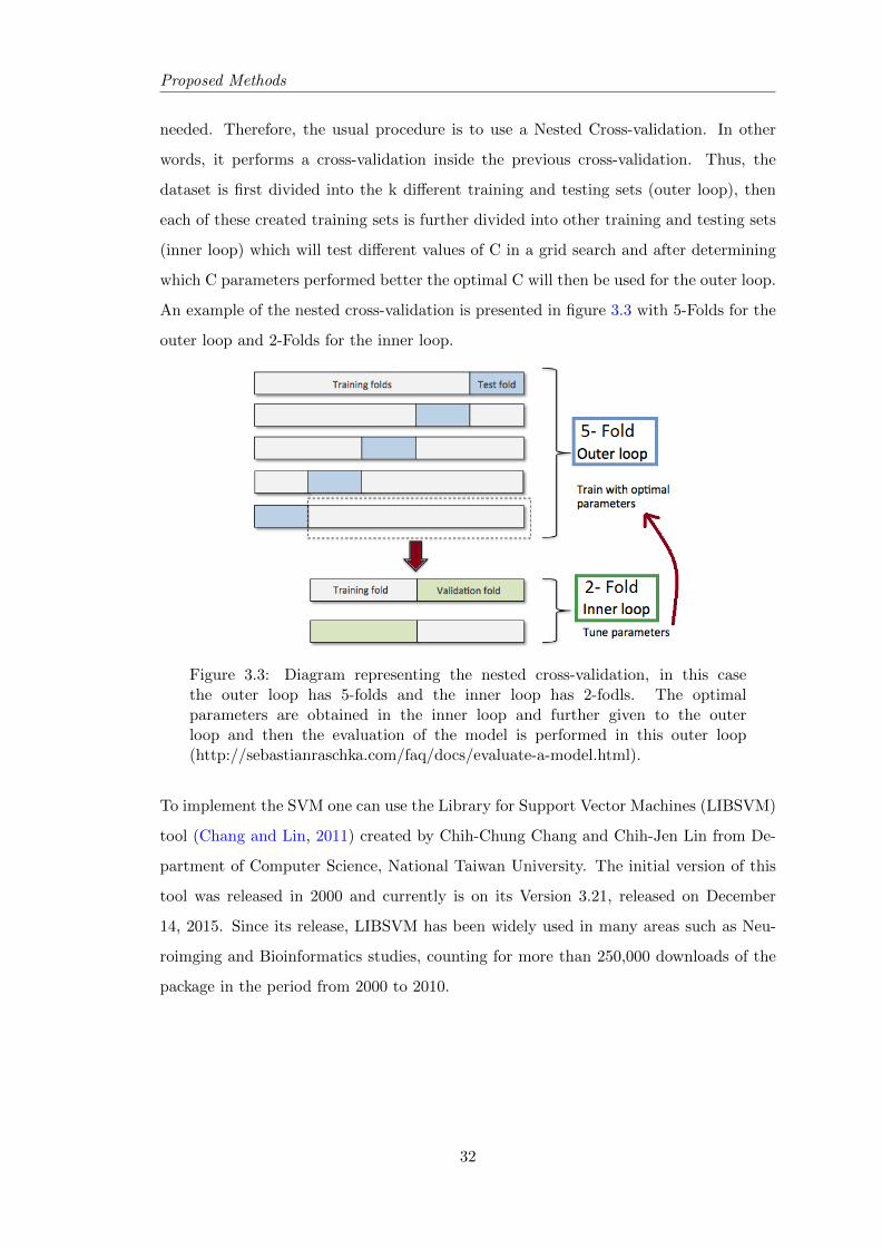
Proposed Methods
needed. Therefore, the usual procedure is to use a Nested Cross-validation. In other
words, it performs a cross-validation inside the previous cross-validation. Thus, the
dataset is first divided into the k different training and testing sets (outer loop), then
each of these created training sets is further divided into other training and testing sets
(inner loop) which will test different values of C in a grid search and after determining
which C parameters performed better the optimal C will then be used for the outer loop.
An example of the nested cross-validation is presented in figure 3.3 with 5-Folds for the
outer loop and 2-Folds for the inner loop.
Figure 3.3: Diagram representing the nested cross-validation, in this casethe outer loop has 5-folds and the inner loop has 2-fodls. The optimalparameters are obtained in the inner loop and further given to the outerloop and then the evaluation of the model is performed in this outer loop(http://sebastianraschka.com/faq/docs/evaluate-a-model.html).
To implement the SVM one can use the Library for Support Vector Machines (LIBSVM)
tool (Chang and Lin, 2011) created by Chih-Chung Chang and Chih-Jen Lin from De-
partment of Computer Science, National Taiwan University. The initial version of this
tool was released in 2000 and currently is on its Version 3.21, released on December
14, 2015. Since its release, LIBSVM has been widely used in many areas such as Neu-
roimging and Bioinformatics studies, counting for more than 250,000 downloads of the
package in the period from 2000 to 2010.
32
Proposed Methods
3.2.2 Logistic Regression
In contrast with SVM, Logistic Regression (LR) is a probabilistic classifier, so the result
of the classification is not the sign which will represent the class label like in SVM,
instead the result will be a probability.
LR is based on the concept of linear regression models, however in this case it has to be
generalised in order to be used for classification. In linear regression models the model
prediction is given by the linear function: y(x) = wTx + b, with y ∈ R, consequently it
would have values ranging [-∞, + ∞]. However, in classification problems, we wish to
predict discrete class labels, or in this case, a posterior probability which will identify
how likely a given sample belongs to the positive or negative class. Therefore the values
of y should be in the interval [0,1], as it corresponds to probability values. In order to
achieve this, the linear function has to suffer some transformation, which is done with a
non-linear function called logistic sigmoid function σ(.), represented by equation σ(a) =
11+exp(−a) . Thus, the probabilities in logistic regression for a given sample belonging to
a positive class are given by equation 3.14. The graphical representation of the sigmoid
function is presented in figure 3.4.
p(wTx + b) =1
1 + e−(wTx+b)(3.14)
Figure 3.4: Representation of the logistic sigmoid function σ(a). Regardless thevalue of a (horizontal axis), the function σ(a) will always return a value in theinterval [0,1].
Plus, this sigmoid function satisfies the following symmetric property: σ(−a) = 1−σ(a);
which allows finding the corresponding probability of the same sample belonging to a
33
Proposed Methods
negative class and is in accordance with the probability property that P(positive class)
+ P(negative class) = 1.
The implementation of this classifier is quite straightforward when using the SLEP
toolbox that was previously used for feature selection. First the SLEP toolbox is used to
determine the weight vector w and the parameter b, then the probabilities are discovered
by using equation 3.14.
As LR returns probabilities, in order to turn these into a discrete label to further use
statistics to evaluate the model prediction performance, a threshold should be defined.
Normally this threshold can be defined as 0.5, meaning that all the test samples with
probabilities inferior to 0.5 are classified as negative and all the ones which are higher
than 0.5 are classified as positive label, the ones with values equal to 0.5 have equal
probability of belonging to positive class and negative class. This means that the clas-
sifier cannot decide which class it should belong to. In these cases, it is possible to
predefine the location of a equal sign in the threshold, which will determinate the class
to attribute for that sample. For example, if one defines that only values higher than
0.5 are seen as positive samples, it implies that values equal or lower will be seen as
negative. In this case, the decision is not made by the classifier instead is the user who
defines it.
3.2.3 Gaussian Process
Gaussian process classifiers are formulated based on the foundation of linear logistic
regression models, more specifically they can be seen as a kernelized Bayesian extension
of the logistic regression model (Young et al., 2013).
3.2.3.1 Bayesian theory
Before starting to explain GP classifier theory, it is useful to understand how the
Bayesian theory is formulated. This theory is known as:
p(h|D) =p(D|h)p(h)
p(D), p(D) 6= 0 (3.15)
34
Proposed Methods
Interpreting equation 3.15 we can say that p(h | D) is the posterior probability, i.e., is
the probability of a hypothesis h after data D is observed; p(h), is the prior probability,
which is the probability of h before any D is observed; and p(D | h) also known as the
likelihood is the probability of D with h fixed.
For most standard Bayesian methods, the prior distribution p(h) is fixed before any
data is observed. However, for GP classifiers as it is a supervised classifier, we want to
determine the statistical inference based on a prior distribution which is estimated from
the data, i.e., empirically. For that reason, in GP classifiers the method used is called
Empirical Bayes method, which is an approximation of the fully Bayesian treatment.
3.2.3.2 Gaussian Process classification formulation
The probability of belonging to a certain class at an input location has a relation with
the value of some latent function f at that location (Young et al., 2013). For the
purpose of determining this probability, GP classifier forms a prior over this latent
function p(f), and then squishes this through the logistic sigmoid function σ(.), as in
logistic regression, to obtain values in the [0,1] interval, guaranteeing valid values for
probabilistic interpretations.
Thus, given a datasetD = (xi, yi)ni=1 with n samples, to obtain the posterior probabilities
mathematically these can be represented by (Williams, 2006):
p(f |D) ∝ p(f)p(D|f) (3.16)
posterior ∝ prior× likelihood (3.17)
In order to perform GP classification and apply a prior over the function values, the
classifier should be first parametrized by a mean function and a covariance function
(equation 3.18).
p(f) = N (mean, cov) (3.18)
35
Proposed Methods
The covariance function plays an important role in GP classifier formulation because
it will define the similarity between data points (samples). Usually, this is achieved
using the linear kernel as the covariance function k, which performs the dot product
between two samples x and x′ and is parametrized by a hyper-parameter θ giving rise
to a covariance matrix K, see equation 3.19. Thus, equation 3.18 can be rewritten as
equation 3.20. This covariance function can then be optimized by determining the proper
hyper-parameter θ via type-II maximum likelihood, also known as Empirical Bayes.
Type-II maximum likelihood maximizes the marginal likelihood which will automatically
incorporates a trade-off between model fit and model complexity (Williams, 2006).
K = k(x,x′) = x · x′ + θ (3.19)
p(f |θ) = N (mean,K) (3.20)
Once the hyper-parameters are defined, the predictions to unseen data are done by in-
tegrating across this prior (Young et al., 2013). However, for classification problems,
because the sigmoid function is used, the exact Bayesian inference is analytically in-
tractable and therefore approximation inference techniques have to be used, in order to
obtain the final desired posterior probability p(f |D, θ). For this purpose, the usual ap-
proximation methods used are the Laplace Approximation (Williams and Barber, 1998)
or the Expectation-Propagation (EP) method (Minka, 2001).
Likewise LR, the GP will also need to define a threshold in order to further transform
these probabilities into class labels for further statistical evaluation.
To implement the GP classifier the Gaussian Processes for Machine Learning (GPML)
Matlab Code version 3.6 was used (Rasmussen and Nickisch, 2015). The code was
written by Carl Edward Rasmussen and Hannes Nickisch and is based on previous
versions written by Carl Edward Rasmussen and Chris Williams. Both Carl Edward
Rasmussen and Chris Williams are the authors of the book Gaussian Processes for
Machine Learning (Rasmussen and Williams, 2006) which explains in detail how GP are
formulated and used for pattern recognition problems. This code runs on both Octave
3.2.x and Matlab 7.x and later.
36
Chapter 4
Methodology and Results
This chapter will present the experiments performed in this thesis and its results along
with the discussion. The first section 4.1 shows the details of the data used, section 4.2
presents the experimental approach tested in this work, finally in section 4.3 the results
and discussion are presented.
4.1 Data
4.1.1 Subjects
All data used in this thesis was collected from the ADNI database and were baseline
scans, i.e. scans corresponding to the subject’s first visit. The total number of subjects
was 210, with 50 belonging to the AD group, 48 to the CN group and 112 to MCI, which
in turn, were further divided into 82 MCI-non converters and 30 MCI-converters, over a
24 month period, by analysing an excel file provided by the ADNI database where the
diagnosis history is presented. The demographic data of these subjects is presented in
Table 4.1.
Prior to classification, some statistical tests on these demographic data are necessary
to make sure that the classification results for the different groups are not influenced
by a significant difference in age populations or by a disproportion of males or females
subjects. Hence, two statistic tests were performed: two sample t-test for age and the
Table 4.1: Distribution of male and female subjects, with total number of sub-jects presented in parenthesis, and mean ages with the respective standard de-viation values for each group.
4.1.1.1 Two sample t-test for age
The two-sample t-test is a test statistic which follows the t-Student’s distribution under
a null hypothesis which states that the means of two independent samples are equal. If
the p-value obtained from this test is lower than a significant level previously defined
(usually 0.05 or 0.1) then the null hypothesis should be rejected. In order to determine
if the various groups of data (AD; MCI; CN; MCI-C; MCI-NC) are significantly different
from each other, in terms of their mean ages (µ), the following the null hypothesis were