1 A MULTISCALE APPROACH IN TOPOLOGY OPTIMIZATION Gr´ egoire ALLAIRE CMAP, Ecole Polytechnique The most recent results were obtained in collaboration with F. de Gournay, F. Jouve, O. Pantz, A.-M. Toader. Topology optimization G. Allaire
Transcript
1
A MULTISCALE APPROACH
IN TOPOLOGY OPTIMIZATION
Gregoire ALLAIRE
CMAP, Ecole Polytechnique
The most recent results were obtained in collaboration with F. de
Gournay, F. Jouve, O. Pantz, A.-M. Toader.
Topology optimization G. Allaire
2
CONTENTS
1. Introduction.
2. Classical method of shape differentiation. Link between ill-posedness and
topology optimization.
3. The level set method.
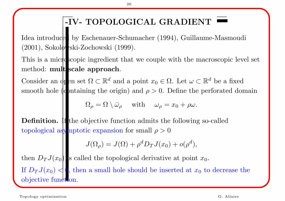
4. The topological gradient.
Topology optimization G. Allaire
3
-I- INTRODUCTION
A shape optimization problem is defined by three data:
a model (a p.d.e.) in order to analyze the mechanical behavior of a
structure,
an objective function which measures one or several performance(s) and
has to be minimized,
an admissible set of shapes (the optimization variables) which takes into
account additional constraints.
For simplicity, we choose to focus on single load optimization in linear
elasticity.
Topology optimization G. Allaire
4
SHAPE OPTIMIZATION
Mathematical formulation : minimize an objective function over a set of
admissibles shapes Ω (including possible constraints)
infΩ∈Uad
J(Ω)
The objective function is evaluated through a partial differential equation
(state equation)
J(Ω) =
∫
Ω
j(uΩ) dx
where uΩ is the solution of
PDE(uΩ) = 0 in Ω
Topology optimization : the optimal topology is unknown.
Topology optimization G. Allaire
5
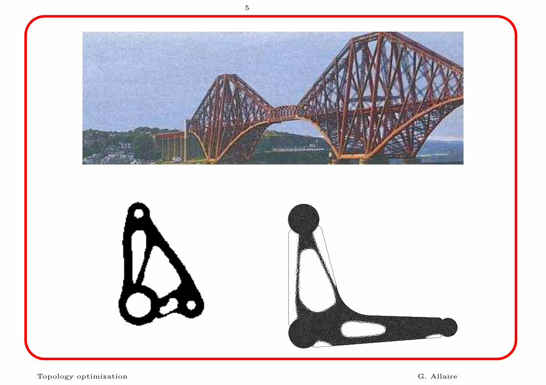
Topology optimization G. Allaire
6
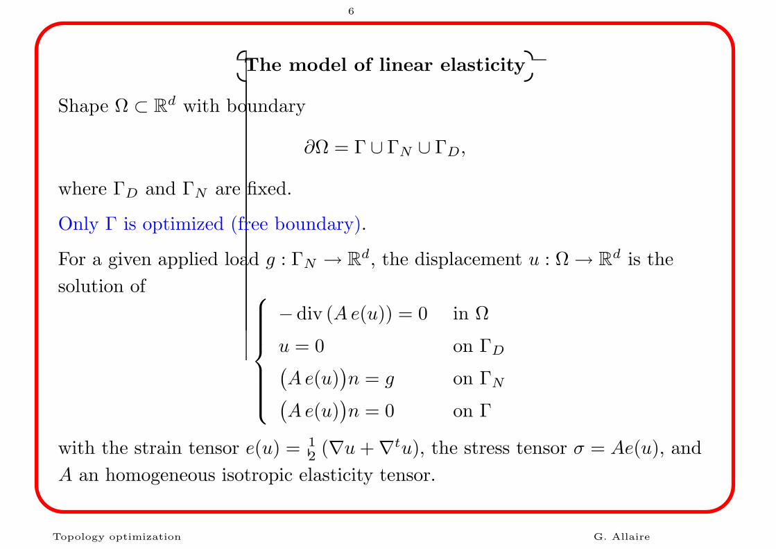
The model of linear elasticity
Shape Ω ⊂ Rd with boundary
∂Ω = Γ ∪ ΓN ∪ ΓD,
where ΓD and ΓN are fixed.
Only Γ is optimized (free boundary).
For a given applied load g : ΓN → Rd, the displacement u : Ω → R
d is the
solution of
− div (Ae(u)) = 0 in Ω
u = 0 on ΓD(
Ae(u))
n = g on ΓN(
Ae(u))
n = 0 on Γ
with the strain tensor e(u) = 12 (∇u+ ∇tu), the stress tensor σ = Ae(u), and
A an homogeneous isotropic elasticity tensor.
Topology optimization G. Allaire
7
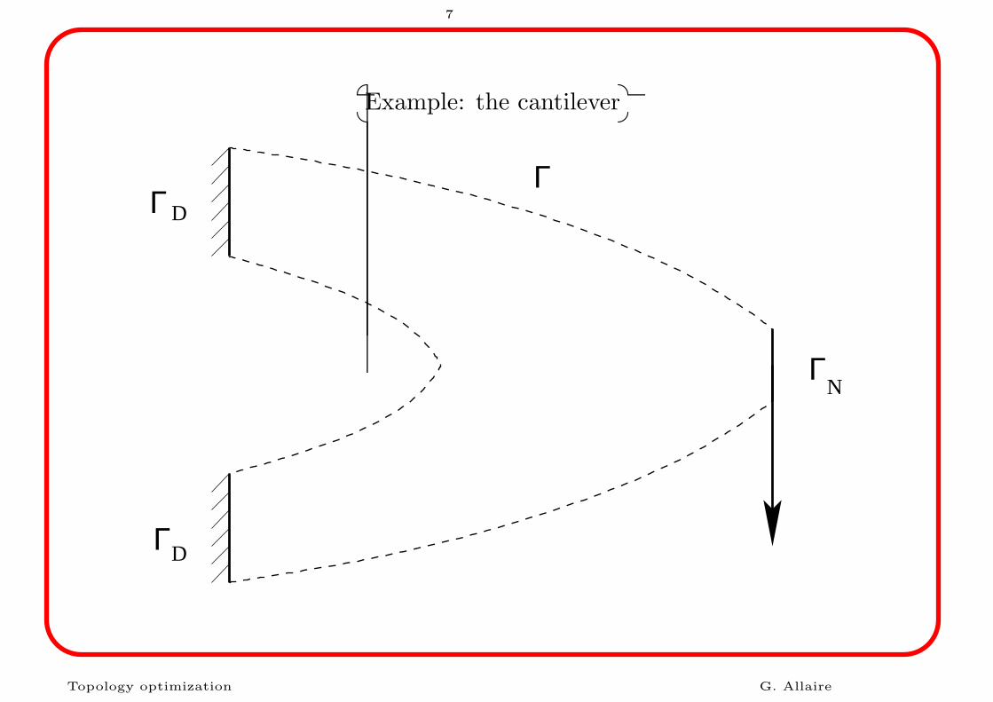
Example: the cantilever
Γ
Γ
Γ
Γ
N
D
D
Topology optimization G. Allaire
8
Admissible set and objective function
The set of admissible shapes is typically
Uad =
Ω ⊂ D open set such that ΓD
⋃
ΓN ⊂ ∂Ω and
∫
Ω
dx = V0
,
where D ⊂ Rd is a given “working domain” and V0 is a prescribed volume.
The shape optimization problem is
infΩ∈Uad
J(Ω),
with, as an objective function, the compliance
J(Ω) =
∫
ΓN
g · u dx,
or a least square criteria for a target displacement u0(x)
J(Ω) =
∫
Ω
k(x)|u− u0|2dx.
The true optimization variable is the free boundary Γ.
Topology optimization G. Allaire
9
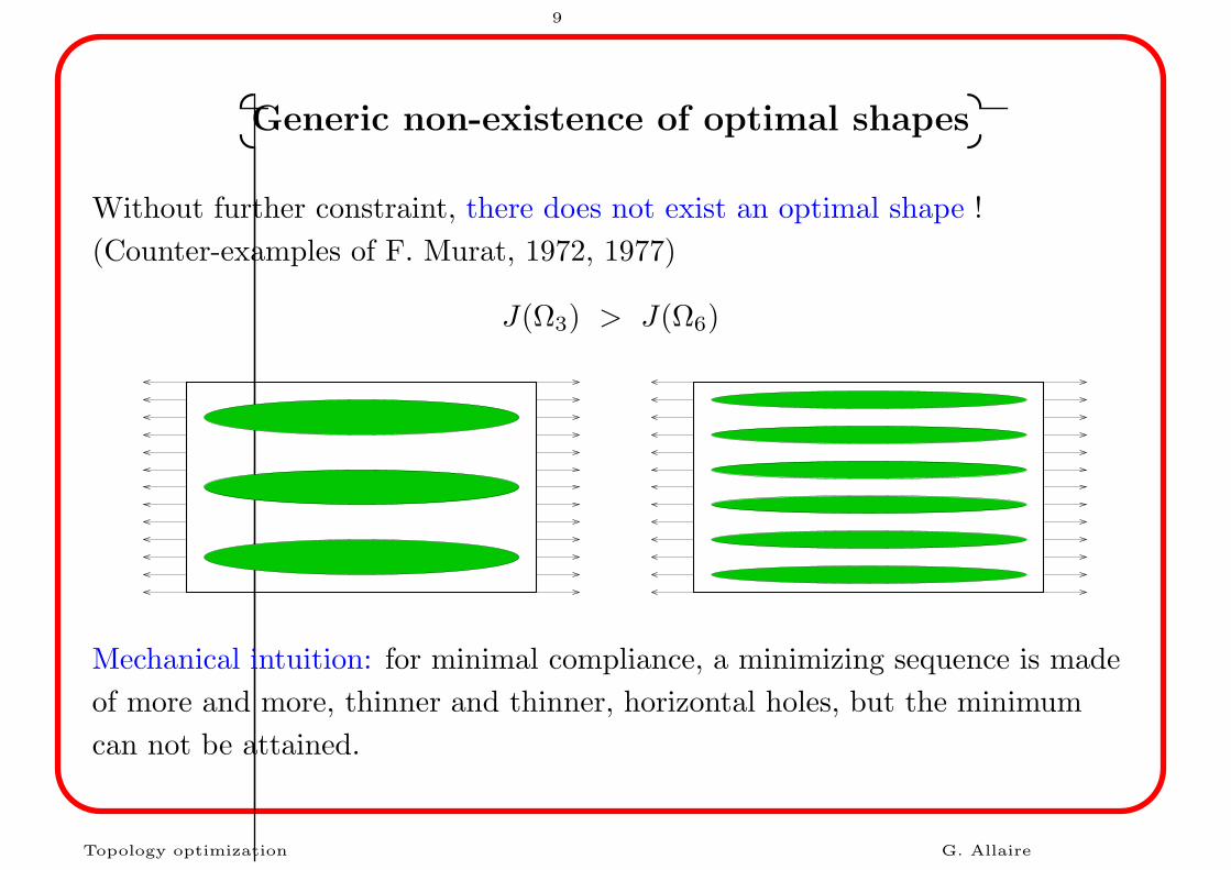
Generic non-existence of optimal shapes
Without further constraint, there does not exist an optimal shape !
(Counter-examples of F. Murat, 1972, 1977)
J(Ω3) > J(Ω6)
Mechanical intuition: for minimal compliance, a minimizing sequence is made
of more and more, thinner and thinner, horizontal holes, but the minimum
can not be attained.
Topology optimization G. Allaire
10
Consequences of ill-posedness
Deep interplay between mathematical and computational issues !
Ill-posedness can be seen numerically in the occurence of many local
minima.
Very often local minima correspond to different topologies.
A microstructure appears in the minimizing sequences.
Need a multiscale approach to numerically solve this difficulty.
Two possible numerical remedies:
1. The homogenization method: composite materials with a microstructure
are introduced (relaxation of the problem).
2. Level set method with a topological gradient: possible topology changes
with a nucleation mechanism for new holes.
Topology optimization G. Allaire
11
-II- SHAPE DIFFERENTIATION
We recall the well-known Hadamard’s method.
Let Ω0 be a reference domain. Shapes are parametrized by a vector field θ
Ω = ( Id + θ)Ω0 with θ ∈W 1,∞(Rd; Rd).
x
Ω (Ι+θ)Ω
x+ (x)θ
00
Topology optimization G. Allaire
12
Shape derivative
Definition: the shape derivative of J(Ω) at Ω0 is the Frechet differential of
θ → J(
( Id + θ)Ω0
)
at 0.
Lemma. For any θ ∈W 1,∞(Rd; Rd) such that ‖θ‖W 1,∞(Rd;Rd) < 1, ( Id + θ) is
a diffeomorphism in Rd. In particular, it implies that there are no topology
variations.
Many authors have contributed to this setting: Hadamard (1907),
Murat-Simon (1976), Pironneau (1984), Sokolowski-Zolesio (1992), etc.
Topology optimization G. Allaire
13
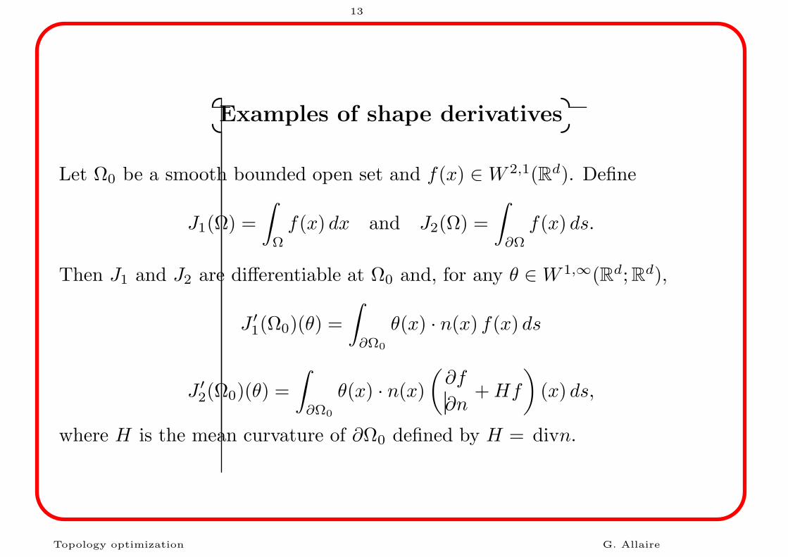
Examples of shape derivatives
Let Ω0 be a smooth bounded open set and f(x) ∈W 2,1(Rd). Define
J1(Ω) =
∫
Ω
f(x) dx and J2(Ω) =
∫
∂Ω
f(x) ds.
Then J1 and J2 are differentiable at Ω0 and, for any θ ∈W 1,∞(Rd; Rd),
J ′1(Ω0)(θ) =
∫
∂Ω0
θ(x) · n(x) f(x) ds
J ′2(Ω0)(θ) =
∫
∂Ω0
θ(x) · n(x)
(
∂f
∂n+Hf
)
(x) ds,
where H is the mean curvature of ∂Ω0 defined by H = divn.
Topology optimization G. Allaire
14
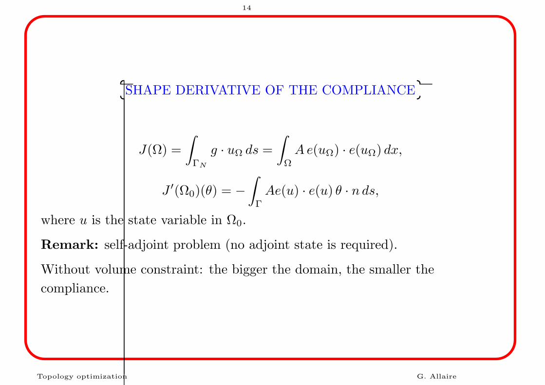
SHAPE DERIVATIVE OF THE COMPLIANCE
J(Ω) =
∫
ΓN
g · uΩ ds =
∫
Ω
Ae(uΩ) · e(uΩ) dx,
J ′(Ω0)(θ) = −
∫
Γ
Ae(u) · e(u) θ · n ds,
where u is the state variable in Ω0.
Remark: self-adjoint problem (no adjoint state is required).
Without volume constraint: the bigger the domain, the smaller the
compliance.
Topology optimization G. Allaire
15
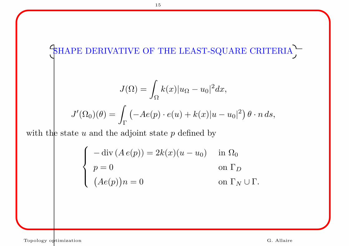
SHAPE DERIVATIVE OF THE LEAST-SQUARE CRITERIA
J(Ω) =
∫
Ω
k(x)|uΩ − u0|2dx,
J ′(Ω0)(θ) =
∫
Γ
(
−Ae(p) · e(u) + k(x)|u− u0|2)
θ · n ds,
with the state u and the adjoint state p defined by
− div (Ae(p)) = 2k(x)(u− u0) in Ω0
p = 0 on ΓD(
Ae(p))
n = 0 on ΓN ∪ Γ.
Topology optimization G. Allaire
16
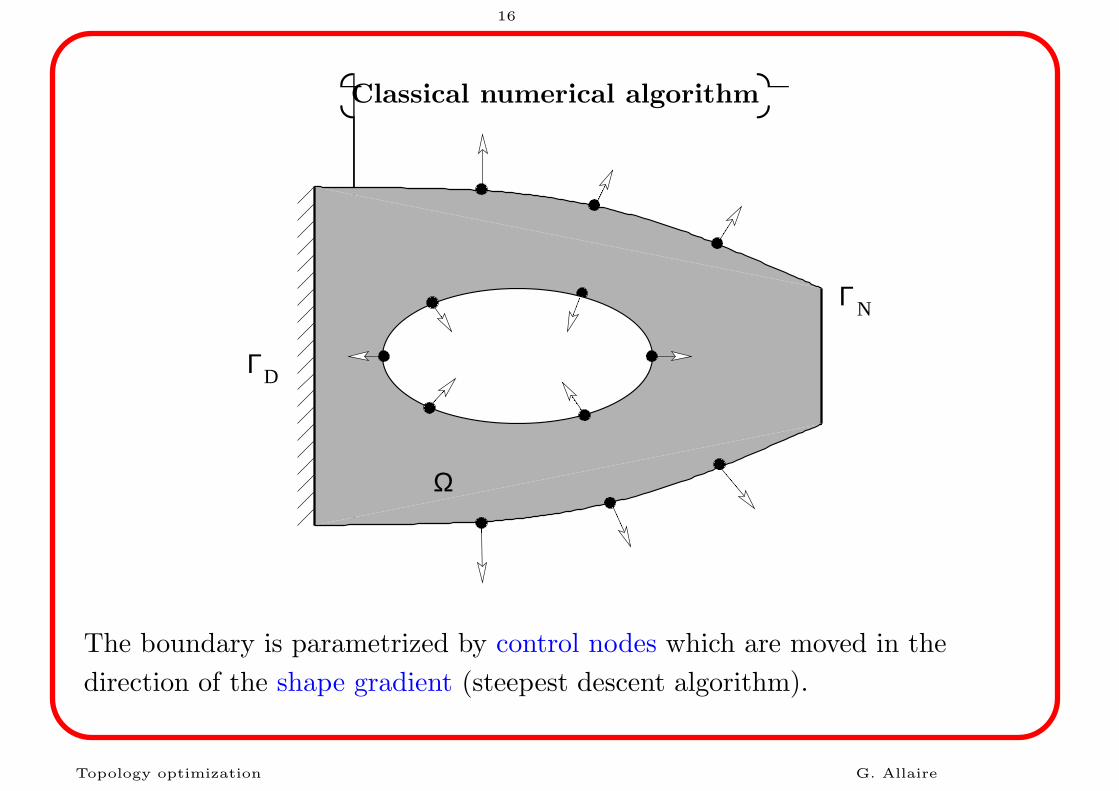
Classical numerical algorithm
! ! !! ! !! ! !! ! !! ! !
" " "" " "" " "" " "" " "Ω
Γ
Γ
D
N
## $$
%% &&
'' ((
)))
***
++ ,,
The boundary is parametrized by control nodes which are moved in the
direction of the shape gradient (steepest descent algorithm).
Topology optimization G. Allaire
17
Principles
Iterative algorithm: the shape derivative is computed (by solving a
p.d.e.), and accordingly the shape is deformed.
Convergence to a local minimum.
Strong influence of the initial design and of the mesh size.
The topology (number of holes in 2-d) can not change.
The shape must be re-meshed in case of large deformations: this is too
costly in 3-d.
Topology optimization G. Allaire
18
NUMERICAL RESULTS
Illustration of ill-posedness: local minima and impossibility of topology
changes. (Results obtained with FreeFem++ in collaboration with O. Pantz.)
Cantilever problem: compliance minimization.
Consequence: we must optimize both the shape and the topology.
Two possible directions (among others):
Relaxation by the homogenization method.
The level set method with a topological gradient.
They both rely on a multiscale approach. We focus on the latter one. (Similar
idea in the context of inverse problems by Burger, Hackl and Ring, JCP 2004).
Topology optimization G. Allaire
19
-III- LEVEL SET METHOD
A new numerical implementation of an old idea...
Still in the framework of Hadamard’s method.
Shape capturing algorithm.
Fixed mesh: low computational cost.
Main tool: the level set method of Osher and Sethian (JCP 1988).
Some references: Sethian and Wiegmann (JCP 2000), Osher and Santosa