A Multivariate Robust Control Chartfor Individual Observations

SHOJA’EDDIN CHENOURI and STEFAN H. STEINER

University of Waterloo, Waterloo, ON N2L 3G1, Canada

ASOKAN MULAYATH VARIYATH

Memorial University of Newfoundland, St.John’s, NL A1C 5S7, Canada

To monitor a multivariate process, a classical Hotelling’s T 2 control chart is often used. However, it

is well known that such control charts are very sensitive to the presence of outlying observations in the

historical Phase I data used to set the control limit. In this paper, we propose a robust Hotelling’s T 2-

type control chart for individual observations based on highly robust and efficient estimators of the mean

vector and covariance matrix known as reweighted minimum covariance determinant (RMCD) estimators.

We illustrate how to set the control limit for the proposed control chart, study its performance using

simulations, and illustrate implementation in a real-world example.

Key Words: Hotelling’s T 2; Multivariate Robust Estimation of Location and Scatter; Multivariate Statistical

Process Control; Outliers; Reweighted Minimum Covariance Determinant Estimators.

MONITORING a process/product over time using acontrol chart allows quick detection (and cor-

rection) of unusual conditions. Control charts are im-plemented in two phases. In Phase I, some historicalprocess data, assumed to come from an in-controlprocess, are used to set the control limit(s). In PhaseII, the process is monitored on an ongoing basis usingthe control limit(s) from Phase I. In Phase II, obser-vations falling outside the control limit(s) or unusualpatterns of observations signal that the process hasshifted from the in-control process settings. Such sig-nals trigger a search for an assignable cause and, ifthe cause is found, lead to corrective action to pre-vent its recurrence.

For many products or processes, overall quality is

Dr. Chenouri is an Assistant Professor in the Depart-

ment of Statistics and Actuarial Science. His email address

is schenouri@uwaterloo.ca.

Dr. Variyath is an Assistant Professor in the Department

of Mathematics and Statistics. His email address is variyath@

mun.ca.

Dr. Steiner is an Associate Professor in the Department

of Statistics and Actuarial Science. He is a Senior Member of

ASQ. His email address is shsteiner@uwaterloo.ca.

defined simultaneously by a number of quality char-acteristics. To monitor a multivariate process in away that takes into account the correlations amongthe variates, we may use a Hotelling’s T 2 controlchart (Hotelling (1947), Tracy et al. (1992)). To im-plement the Hotelling’s T 2 control chart in Phase Iwith n observations, for each individual observationj we calculate

T 2(j) = (xj − x)′C−1(xj − x), (1)

where xj = (xj1, . . . , xjp)′, j = 1, . . . , n, are the np−variate Phase I observations with sample meanx = n−1

∑ni=1 xi and covariance matrix C = (n −

1)−1∑n

i=1(xi−x)(xi−x)′. For each individual obser-vation, we compare T 2(j) with a control limit usuallyderived by assuming the xj ’s are independent multi-variate normal, i.e., MVNp(μ,Σ), with mean μ andcovariance matrix Σ. Note that, in this paper, wedo not consider the situation where observations arecorrelated over time. Under these normality and in-dependence assumptions, the control limit for PhaseI data is based on a Beta distribution and an F distri-bution for a Phase II observation that is independentof the Phase I data (see Tracy et al. (1992)). A largevalue of T 2(j) indicates that the process has shiftedin some way.

Vol. 41, No. 3, July 2009 259 www.asq.org

260 SHOJA’EDDIN CHENOURI, ASOKAN MULAYATH VARIYATH, AND STEFAN H. STEINER

To motivate and illustrate this work, consider thefinal assembly of automobiles. A critical character-istic of each automobile, which can influence cus-tomer perception of quality, is alignment. One mea-sure of alignment depends on four angles, namelyfront-right, and front-left wheel camber and caster.In this example, large volumes of data are collectedbecause final 100% inspection includes measurementof the four camber and caster angles. Automobileswith any of the characteristics out of specificationare reworked before shipment. To monitor the align-ment process, we can use a multivariate control chart,such as a Hotelling’s T 2 chart. However, the processproduces the occasional outlier or flyer (that are re-worked before shipment). As a result, it would beuseful to have a control-chart setup procedure thatis robust to outliers.

As in the alignment example, the assumption thatthe Phase I data comes from an in-control process isnot always valid. Unusual observations in Phase I canlead to inflated control limits and reduced power todetect process changes in Phase II. For this reason,part of Phase I consists of the retrospective applica-tion of the control chart with the determined controllimit(s) to the Phase I process data. Any Phase Iobservations outside the control limit(s) are investi-gated. If found to be due to an identified assignablecause that can be removed, the observation is elim-inated and the control limit(s) recalculated. This it-erative re-estimation procedure in Phase I can elim-inate the effect of a small number of very extremeobservations but will fail to detect more moderateoutliers. For this reason, in Phase I, we propose touse robust estimators of the mean vector and covari-ance matrix in order to determine an appropriatecontrol limit for Phase II data.

As shown in Equation (1), Hotelling’s T 2 uses theclassical sample mean and sample covariance matrixto estimate the population mean vector and covari-ance matrix. However, the sample mean vector andcovariance matrix estimators are very sensitive tooutliers in the Phase I data. Thus, Hotelling’s T 2

suffers from a masking effect, where multiple out-liers in the Phase I data yield T 2 values that arenot large or unusual (Rousseeuw and van Zomeren(1990)). Sullivan and Woodall (1996, 1998) showedthat, in certain situations, the T 2 statistic with thesample covariance matrix estimator is not effectivein detecting shifts in the process mean vector. Theyproposed several different estimators of the covari-ance matrix and concluded that an estimator based

on successive differences is more effective in detectingthe process shift when certain conditions apply.

Vargas (2003) introduced robust control charts foridentifying outliers in Phase I multivariate individ-ual observations based on two robust estimates ofmean vector and covariance matrix, namely, the min-imum covariance determinant (MCD) and the min-imum volume ellipsoid (MVE). The exact distribu-tion of T 2 with robust estimators based on MVE andMCD is not available, so control limits for Phase Idata need to be obtained empirically. Vargas (2003)and Jensen et al. (2007) estimated the control lim-its for the robust T 2 charts for Phase I data basedon simulations. Jensen et al. (2007) tabulated theseestimates for sample sizes of n = 10, . . . 100, dimen-sions p = 2, . . . 10, and an overall confidence level of1−α = 0.95 for any out-of-control points in Phase I.The performance of these robust control charts wasassessed in terms of the probability of a signal (i.e.,detecting an outlier) in Phase I only.

Our approach to the problem of monitoring themultivariate observations differs in two ways fromVargas (2003) and Jensen et al. (2007). We pro-pose using robust estimators of the mean vectorand the covariance matrix based on the reweightedMCD (Rousseeuw and Van Zomeren (1990), Lop-uhaa and Rousseeuw (1991), Willems et al. (2002)).Reweighted MCD estimators inherit the nice proper-ties of initial MCD estimators, such as affine equiv-ariance, robustness, and asymptotic normality, whileachieving a higher efficiency. Reweighted MCD esti-mates are not unduly influenced by the outliers andthus there is no need to identify outliers in the PhaseI data, which is reflected in our simulations results.Second, we propose robust control charts for PhaseII data based on the reweighted MCD estimates ofthe mean vector and covariance matrix from PhaseI. Our simulation studies show that the robust con-trol chart based on the reweighted MCD estimateshas better performance than other existing controlcharts under certain conditions.

Organization of the remaining part of the paperis as follows. In the next section, we discuss the ex-isting robust estimation methods. Following that, weformally introduce a robust control chart based onthe reweighted MCD. The estimation of distributionquantiles using Monte Carlo methods needed to setthe control limit is then presented. Following that,we compare the performance of reweighted MCD andother previously proposed robust control charts usingsimulations. Then the reweighted MCD control chart

Journal of Quality Technology Vol. 41, No. 3, July 2009

A MULTIVARIATE ROBUST CONTROL CHART FOR INDIVIDUAL OBSERVATIONS 261

is applied to the alignment example. A discussionand final conclusions are given in the last section.

Some Background onRobust Estimation

Consider the problem of estimating the parame-ters μ and Σ based on a random sample x1, . . . ,xn

from a p-variate normal MVNp(μ,Σ) distribution. Itis desirable that the estimators are independent ofthe choice of coordinate system. More formally, theestimators tn and Cn of μ and Σ, respectively, arecalled affine equivariant if, for any nonsingular p× pmatrix A and vector b ∈ R

p,

tn(Ax1 + b, . . . ,Axn + b) = Atn(x1, . . . ,xn) + b

Cn(Ax1 + b, . . . ,Axn + b) = ACn(x1, . . . ,xn)A′.

(2)

The finite sample breakdown point, introduced byDonoho and Huber (1983), is a very popular globalmeasure of robustness. Intuitively, it is the smallestamount of contamination necessary to upset an es-timator entirely. Formally, let X

(o) = {x1, . . . ,xn}be a random sample of n observations and tn(X(o))the corresponding estimator. Imagine replacing m ar-bitrary points in X

(o) by arbitrary values. Let thenew data be represented by X

(m). The finite samplebreakdown point of the estimator tn for sample X

(o)

is

ε∗n(tn, X(o))

= min{

m

n; sup

X(m)‖tn(X(m)) − tn(X(o))‖ = ∞

},

(3)

where ‖ · ‖ is the Euclidean norm.

If ε∗n(tn, X(o)) is independent of the initial sampleX

(o), we say the estimator tn has the universal finitesample breakdown point ε∗n(tn). In this case, we cancalculate the limit ε∗ = limn→∞ ε∗n(tn), which is of-ten called the breakdown point or, sometimes, theasymptotic breakdown point. A higher breakdownpoint implies a more robust estimator. For example,for univariate data,

• The mean x has ε∗n(x) = 1/n and hence break-down point ε∗ = 0.

• For odd sample sizes n, the median x =x((n+1)/2) has ε∗n(x) = (n + 1)/2n and hencebreakdown point ε∗ = 1/2.

Relaxing the affine equivariance condition of estima-tors to invariance under the orthogonal transforma-

tion makes it easy to find an estimator with the high-est possible breakdown point 1/2. But, if we are inter-ested in finding an affine equivariant estimator and,at the same time, a robust one, things get compli-cated. The combination of affine equivariance andhigh breakdown is rare. Davies (1987) showed thatthe largest attainable finite sample breakdown pointof any affine equivariant estimator of the location andscatter matrix is �(n − p + 1)/2�/n.

Classical estimators of μ and Σ, i.e., the sample-mean vector and covariance matrix, are affine equiv-ariant but their finite sample breakdown point is1/n. This means that only one outlier can cor-rupt the estimators. Several multivariate robustestimators of μ and Σ have been proposed inthe literature. Examples include the M-estimators(Maronna (1976)), the Stahel–Donoho estimators(Stahel (1981), Donoho (1982)), the S-estimators(Rousseeuw and Yohai (1984), Davies (1987), Lop-uhaa, (1989)), the minimum volume ellipsoid (MVE)and minimum covariance determinant (MCD) esti-mators (Rousseeuw (1985)). The M-estimators arecomputationally cheap, but their breakdown point,under some general conditions, cannot exceed 1/(p+1) (Maronna (1976), Huber (1981)). This upperbound is disappointingly low in high dimension.

The Stahel–Donoho estimators are projectionbased, are reasonably efficient, and have finite samplebreakdown point �(n−2p+2)/2�/n (Donoho (1982)).They are the first affine equivariant estimators withthe highest possible breakdown point, ε∗ = 1/2. Onemajor trouble with Stahel–Donoho estimators is thatthey are computationally expensive.

The S-estimators can attain a finite sample break-down point of �(n − p + 1)/2�/n, with ε∗ = 1/2,under suitable conditions (Lopuhaa and Rousseeuw(1991)). However, these estimators are also very ex-pensive to compute.

The MVE and MCD are two affine equivari-ant estimators introduced by Rousseeuw (1985) thathave finite sample and asymptotic breakdown points�(n − p + 1)/2�/n and 1/2, respectively. The MVElocation estimator has a slow, n−1/3, rate of con-vergence and a nonnormal asymptotic distribution(Davies (1992)). In addition, there is no existingfast algorithm to compute the MVE estimators. TheMCD location and scatter estimators have a n−1/2

rate of convergence, and the former has an asymp-totic normal distribution (Butler et al. (1993)). A fast

Vol. 41, No. 3, July 2009 www.asq.org

262 SHOJA’EDDIN CHENOURI, ASOKAN MULAYATH VARIYATH, AND STEFAN H. STEINER

algorithm is available in standard software packagesto compute MCD estimators in high dimensions.

In this paper, we consider a modified and moreefficient version of the MCD estimators of locationand scatter. To begin, we formally define the MCDestimators. Let x1, . . . ,xn be a random sample takenfrom an absolutely continuous distribution F in R

p.The MCD estimators of location and scatter of thedistribution are determined by the subset of sizeh = �nγ� (where 0.5 ≤ γ ≤ 1), the covariance ma-trix of which has the smallest possible determinant.The MCD location estimate xMCD is defined as theaverage of this subset of h points, and the MCD scat-ter estimate is given by SMCD = an

γ,pCMCD, whereCMCD is the covariance matrix of the subset; the con-stant an

γ,p is cγ,p × bnγ,p, where cγ,p is a consistency

factor (see Croux and Haesbroeck (1999)); and bnγ,p

is a finite sample correction factor (see Pison et al.(2002)). Here 1−γ represents the (asymptotic) break-down point of the MCD estimators, i.e., ε∗ = 1 − γ.

The MCD estimator has its highest possible finite-sample breakdown point when h = �(n + p +1)/2� (see Rousseeuw and Leroy (1987)). Comput-ing the exact MCD estimators (xMCD,SMCD) isvery expensive or even impossible for large samplesizes in high dimensions (see Woodruff and Rocke(1994)). However, various algorithms have been sug-gested for approximating the MCD. A fast algorithmwas proposed independently by Hawkins and Olive(1999) and Rousseeuw and Van Driessen (1999). Forsmall datasets, the algorithm of Rousseeuw and VanDriessen (1999), known as FAST-MCD, typicallyfinds the exact MCD, whereas, for larger datasets,it is an approximation. The FAST-MCD is imple-mented in standard statistical softwares such asSPLUS, R, SAS, and Matlab.

For the multivariate normal distribution

MVNp(μ,Σ),

the MCD estimator (xMCD,SMCD) with

cγ,p = γ/P (χ2(p+2) ≤ qγ)

is consistent for (μ,Σ), where χ2(r) represents a chi-

square random variable with r degrees of freedomand qγ is the γth quantile of χ2

(r).

In addition to being highly robust against out-liers, if robust multivariate estimators are going tobe of use in statistical inference, they should offerreasonable efficiency under the multivariate normaldistribution. There is usually a tradeoff between ef-ficiency and robustness, but if one is interested in

having both efficiency and robustness, the best pro-posal seems to be two-stage or reweighted estima-tors (Rousseeuw and van Zomeren (1990), Woodruffand Rocke (1994)). In this paper, we propose usingreweighted MCD estimators as commonly defined inthe literature (Willems et al. (2002)). This is becausethe reweighted MCDs are affine equivariant estima-tors with a high breakdown point, an n−1/2 rate ofconvergence, high efficiency, and there exists a fastand good approximate algorithm for computationalpurposes. The reweighted MCD estimators of μ andΣ are the weighted-mean vector,

xRMCD =

(n∑

i=1

wixi

)/ (n∑

i=1

wi

), (4)

and covariance matrix,

SRMCD

= cη,pdn,pγ,η

n∑i=1

wi(xi − xRMCD)(xi − xRMCD)′

n∑i=1

wi

,

(5)

where the weights are based on the robust distances

D(xi) =√

(xi − xMCD)′S−1MCD(xi − xMCD). (6)

Observations with D(xi) below the cutoff value qη,where qη is the ηth quantile of the chi-square distri-bution with p degrees of freedom, are assigned weight1, while all other observations are given weight 0, i.e.,

wi ={

1 if D(xi) ≤ qη

0 otherwise.(7)

We use the value η = 0.975, which was advocated andused by Rousseeuw and Van Driessen (1999). Usingcη,p = η/P (χ2

(p+2) ≤ qη) makes SRMCD consistentunder the multivariate normal distribution. The fac-tor dn,p

γ,η is a finite sample correction given by Pisonet al. (2002).

The reweighted MCD estimators preserve the fi-nite sample breakdown point of the MCD estima-tors (Lopuhaa and Rousseeuw (1991)). Because theMCD estimators are affine equivariant and the robustdistance D(xi) is invariant under an affine transfor-mation of xi, the reweighted MCD estimators areaffine equivariant. In addition, the reweighted MCDestimators have bounded influence functions and areasymptotically normal, just like the MCDs. In sum-mary, the reweighted MCD estimators inherit thenice properties of the initial MCD estimators, such as

Journal of Quality Technology Vol. 41, No. 3, July 2009

A MULTIVARIATE ROBUST CONTROL CHART FOR INDIVIDUAL OBSERVATIONS 263

affine equivariance, robustness, and asymptotic nor-mality while achieving a higher efficiency. The choiceof γ = 0.5 yields the maximum asymptotic break-down point for the MCD and reweighted MCD esti-mators, i.e., ε∗ = 1 − γ = 0.5.

A Robust Control Chart

Let {x1, . . . ,xn} be a p-variate random sample ofsize n from MVNp(μ,Σ) that is considered the PhaseI data in what follows. It is well known (see Wilks(1963), p. 263) that, for a Phase II observation xf /∈{x1, . . . ,xn}, we have

T 2(f) ∼[p(n + 1)(n − 1)

n(n − p)

]F (p, n − p), (8)

where T 2(f) is as defined in Equation (1) andF (r1, r2) is F distribution with r1 and r2 degreesof freedom. To robustify the T 2 control chart basedon Phase I data, we propose to replace x and S, theclassical estimators of μ and Σ, by the reweightedMCD estimators. Suppose xRMCD and SRMCD rep-resent the reweighted MCD mean vector and covari-ance matrix estimators, respectively. We define a ro-bust Hotelling’s T 2 for xf based on these RMCDestimates by

T 2RMCD(f) = (xf − xRMCD)′S−1

RMCD(xf − xRMCD),(9)

where f = n + 1, n + 2, . . .. The finite sample dis-tributions of the MCD and reweighted MCD esti-mators and thus T 2

MCD(f) and T 2RMCD(f) are un-

known. Asymptotic properties of these estimatorshave been investigated in Butler et al. (1993), Croux,and Haesbroeck (1999), and Lopuhaa (1999). Tofind the asymptotic distribution of T 2

RMCD(f), wefirst note that xRMCD and SRMCD are consistentestimators of μ and Σ, respectively. Furthermore,xf ∼ MVNp(μ,Σ), thus applying the Slutsky the-orem (see Serfling (1980)), as n → ∞

(xf − xRMCD)′S−1RMCD(xf − xRMCD)

D→ (xf − μ)′Σ−1(xf − μ) ∼ χ2(p), (10)

i.e., T 2RMCD(f) has an asymptotic χ2

(p) distribution.However, this asymptotic distribution only works forlarge sample sizes. In the next section, we applyMonte Carlo simulations to estimate quantiles of thedistribution of T 2

RMCD(f) for several combinations ofsample size and dimension. For each dimension, wefurther fit a smooth curve between the sample sizeand quantiles of T 2

RMCD(f). These fits can be usedto estimate appropriate quantiles of T 2

RMCD(f) forsmall Phase I sample sizes (n ≤ 200).

Construction Procedures

Estimation of Control Limits

In order to estimate the 99%, and 99.9% quan-tiles of T 2

RMCD(f) for a given Phase I sample size n,dimension p, and breakdown point 1 − γ, we gener-ate K = 10,000 samples of size n from a standardmultivariate normal distribution MVNp(0, Ip). Foreach data set of size n, we compute the reweightedMCD mean vector and covariance matrix estimates,xRMCD(k), and SRMCD(k), k = 1, . . . K. In addi-tion, for each data set, we randomly generate a newobservation xf,k from MVNp(0, Ip) (treated as aPhase II observation) and calculate the correspond-ing T 2

RMCD(k, f) value as given by Equation (9). Theempirical distribution function of T 2

RMCD(f) is basedon the simulated values

T 2RMCD(1, f), T 2

RMCD(2, f), . . . , T 2RMCD(K, f). (11)

By inverting the empirical distribution function ofT 2

RMCD(f), we obtain Monte Carlo estimates of the99%, and 99.9% quantiles. We construct the empiri-cal distribution of T 2

RMCD(f) for any combination ofp = 2, . . . , 10 and n = 20, 21, . . . , 50, 55, 60, . . . , 200.

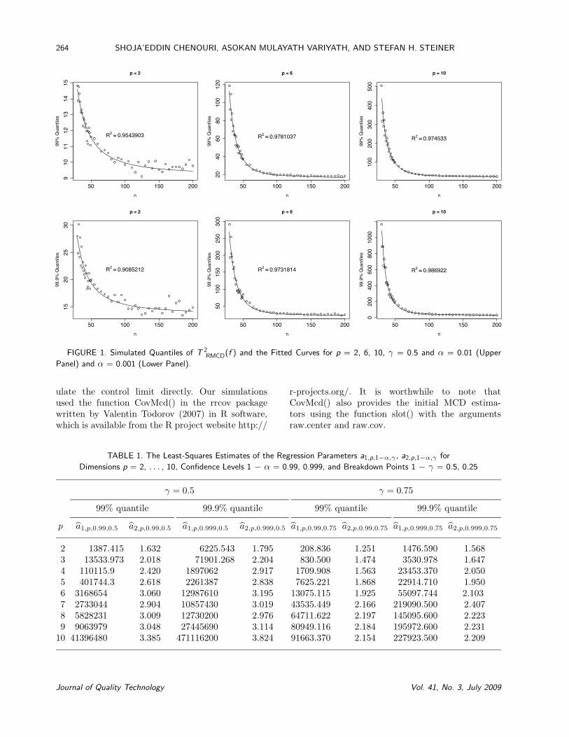
Figure 1 shows scatter plots of the empirical 99%,and 99.9% quantiles of T 2

RMCD(f) versus the sam-ple size n for dimensions p = 2, 6, and 10. Thesescatter plots for different dimensions suggest that wecould model the quantiles using a family of regressioncurves of the form f(n) = b1 + b2/nb3 . Because theasymptotic distribution of T 2(f) is χ2

(p), it is sensibleto use the following two parameter family of curvesinstead:

fp,1−α,γ(n) = χ2(p,1−α) +

a1,p,1−α,γ

na2,p,1−α,γ, (12)

where χ2(p,1−α) is the 1 − α quantile of the χ2 dis-

tribution with p degrees of freedom and a1,p,1−α,γ

and a2,p,1−α,γ are constants. Fitting this curve tothe data will help us predict the desired quantilesof T 2

RMCD(f) for any Phase I sample size n. Notethat, as n increases, fp,1−α,γ(n) approaches χ2

(p,1−α).Table 1 gives the least-square estimates of the pa-rameters a1,p,1−α,γ and a2,p,1−α,γ , for dimensionsp = 2, 3, . . . 10 and the 99%, 99.9% quantiles. UsingTable 1 and Equation (12), we can compute the 99%and 99.9% quantiles of T 2

RMCD(f) for p = 2, . . . , 10and any Phase I sample size n. The regression curvesgiven by Equation (12) fit well to all the cases inTable 1, yielding R2 values of at least 88%. For di-mensions p ≥ 11, a similar pattern is expected, al-though for a given situation, a practitioner may sim-

Vol. 41, No. 3, July 2009 www.asq.org

264 SHOJA’EDDIN CHENOURI, ASOKAN MULAYATH VARIYATH, AND STEFAN H. STEINER

FIGURE 1. Simulated Quantiles of T 2RMCD(f ) and the Fitted Curves for p = 2, 6, 10, γ = 0.5 and α = 0.01 (Upper

Panel) and α = 0.001 (Lower Panel).

ulate the control limit directly. Our simulationsused the function CovMcd() in the rrcov packagewritten by Valentin Todorov (2007) in R software,which is available from the R project website http://

r-projects.org/. It is worthwhile to note thatCovMcd() also provides the initial MCD estima-tors using the function slot() with the argumentsraw.center and raw.cov.

TABLE 1. The Least-Squares Estimates of the Regression Parameters a1,p,1−α,γ , a2,p,1−α,γ for

Dimensions p = 2, . . . , 10, Confidence Levels 1 − α = 0.99, 0.999, and Breakdown Points 1 − γ = 0.5, 0.25

γ = 0.5 γ = 0.75

99% quantile 99.9% quantile 99% quantile 99.9% quantile

p a1,p,0.99,0.5 a2,p,0.99,0.5 a1,p,0.999,0.5 a2,p,0.999,0.5 a1,p,0.99,0.75 a2,p,0.99,0.75 a1,p,0.999,0.75 a2,p,0.999,0.75

2 1387.415 1.632 6225.543 1.795 208.836 1.251 1476.590 1.5683 13533.973 2.018 71901.268 2.204 830.500 1.474 3530.978 1.6474 110115.9 2.420 1897062 2.917 1709.908 1.563 23453.370 2.0505 401744.3 2.618 2261387 2.838 7625.221 1.868 22914.710 1.9506 3168654 3.060 12987610 3.195 13075.115 1.925 55097.744 2.1037 2733044 2.904 10857430 3.019 43535.449 2.166 219090.500 2.4078 5828231 3.009 12730200 2.976 64711.622 2.197 145095.600 2.2239 9063979 3.048 27445690 3.114 80949.116 2.184 195972.600 2.231

10 41396480 3.385 471116200 3.824 91663.370 2.154 227923.500 2.209

Journal of Quality Technology Vol. 41, No. 3, July 2009

A MULTIVARIATE ROBUST CONTROL CHART FOR INDIVIDUAL OBSERVATIONS 265

Implementation Procedures

A step-by-step approach for constructing a T 2RMCD

control chart is given as follows:

Phase I

1. Decide on the sample size n, number of vari-ables p, and confidence level 1 − α.

2. Collect the Phase I data {x1,x2, . . . ,xn} atwell-defined periodic intervals.

3. Using the Phase I data, compute the reweightedMCD estimates xRMCD and SRMCD withbreakdown point 1 − γ = 0.5 or 0.25.

4. For the desired α and p values, choose the least-square estimates a1,p,1−α,γ and a2,p,1−α,γ fromTable 1, and then compute the control limitusing Equation (12).

Phase II

5. Compute T 2RMCD for each of the new observa-

tion as per Equation (9) and plot it on a controlchart with the limit derived in Phase I (step 4).

6. Interpret the chart and look for out-of-controlpoints or patterns. Diagnose the process ifneeded.

Performance ofRobust T2 Control Charts

In order to assess the performance of T 2RMCD con-

trol charts, we conduct a number of simulation stud-ies that consider different Phase I data structuresand the amount of shift in the process mean vectorin the Phase II data. The performance of the controlchart is judged based on the probability of detectingchanges in the process behavior based on the Phase IIdata. A shift in the process mean vector is measuredby the noncentrality parameter (ncp) δ2 as

δ2 = (μ − μA)′Σ−1(μ − μA), (13)

where μ and μA represent in-control and out-of-

control mean vectors, respectively. In this paper,we assume that there are no changes in covari-ance structure. Without loss of generality, because ofaffine equivariance, we generate in-control (no out-lier) Phase I data from the standard multivariatenormal distribution MVNp(0, Ip). In Phase I, 100π%of the data are generated from MVNp(μI , Ip) and100(1 − π)% from MVNp(0, Ip), where δ2

I = ‖μI‖2

and π = 0, 0.10, 0.20. Phase II data are generatedfrom MVNp(μII , Ip) where δ2

II = ‖μII‖2. We consid-ered the following different cases in our performancestudies. We consider each combination of the abovePhase I and II scenarios for Phase I sample sizesn = 50, 150, dimensions p = 2, 6, 10, and breakdownpoints 1−γ = 0.5, 0.25, with the control limit set fora level of confidence of 1 − α = 0.99. We presentonly the result for α = 0.01 here and note thatsimilar conclusions hold for other values of α. Theperformance of the control charts is judged by theprobability of signal that is estimated as the propor-tion of T 2

RMCD(f) values that fall above the controllimit based on 10,000 simulations. In each simula-tion, we generate a sample of size n and compute thereweighted MCD estimates. Using these estimates,we compute the T 2

RMCD(f) from Equation (9) foreach observation in the Phase II data. The computedT 2

RMCD(f) values were then compared with the ap-proximate control limit to estimate the probabilityof signal. This is done for breakdown points of 50%and 25%, and the respective probabilities of signalare denoted by Re-MCD50 and Re-MCD75 in Fig-ures 2–6.

For comparison purposes, we also estimate theprobability of signal, on the same data sets, for othermethods, such as the standard T 2 chart, the robustT 2 chart based on raw MCD and MVE estimatorsdiscussed in Vargas (2003) and Jensen et al. (2007),to identify outliers in Phase I data. We extend theraw MCD and MVE approaches to Phase II by usingthe robust estimators on the Phase I data to elim-inate outliers. Then we construct the standard T 2

TABLE 2. Different Data Cases in the Performance Study

Case Phase I Phase II

1 No outliers (π = 0) Process shifted with δ2II = 0, 5, 10, 15, 20, 25, 30

2 10% (π = 0.10) of the data from δ2I = 5 Process shifted with δ2

II = 0, 5, 10, 15, 20, 25, 303 10% (π = 0.10) of the data from δ2

I = 30 Process shifted with δ2II = 0, 5, 10, 15, 20, 25, 30

4 20% (π = 0.20) of the data from δ2I = 5 Process shifted with δ2

II = 0, 5, 10, 15, 20, 25, 305 20% (π = 0.20) of the data from δ2

I = 30 Process shifted with δ2II = 0, 5, 10, 15, 20, 25, 30

Vol. 41, No. 3, July 2009 www.asq.org

266 SHOJA’EDDIN CHENOURI, ASOKAN MULAYATH VARIYATH, AND STEFAN H. STEINER

●

●

●

●

●● ●

0 5 10 15 20 25 30

0.0

0.2

0.4

0.6

0.8

1.0

p = 2

Phase II non−centrality parameter δδII2

Pro

babi

lity

of s

igna

l

● StandardMVE50MCD50Re−MCD50Re−MCD75

●

●

●

●

●

●

●

0 5 10 15 20 25 30

0.0

0.2

0.4

0.6

0.8

1.0

p = 6

Phase II non−centrality parameter δδII2

Pro

babi

lity

of s

igna

l

● StandardMVE50MCD50Re−MCD50Re−MCD75

●●

●

●

●

●

●

0 5 10 15 20 25 30

0.0

0.2

0.4

0.6

0.8

1.0

p = 10

Phase II non−centrality parameter δδII2

Pro

babi

lity

of s

igna

l

● StandardMVE50MCD50Re−MCD50Re−MCD75

●

●

●

●

●● ●

0 5 10 15 20 25 30

0.0

0.2

0.4

0.6

0.8

1.0

p = 2

Phase II non−centrality parameter δδII2

Pro

babi

lity

of s

igna

l

● StandardMVE50MCD50Re−MCD50Re−MCD75

●

●

●

●

●

●●

0 5 10 15 20 25 30

0.0

0.2

0.4

0.6

0.8

1.0

p = 6

Phase II non−centrality parameter δδII2

Pro

babi

lity

of s

igna

l

● StandardMVE50MCD50Re−MCD50Re−MCD75

●

●

●

●

●

●

●

0 5 10 15 20 25 30

0.0

0.2

0.4

0.6

0.8

1.0

p = 10

Phase II non−centrality parameter δδII2

Pro

babi

lity

of s

igna

l

● StandardMVE50MCD50Re−MCD50Re−MCD75

FIGURE 2. Probability of Signal When the Phase I Data Sets of Size n = 50 (Upper Panel) and n = 150 (Lower Panel)

Are Outlier Free (See Case 1 in Table 2).

FIGURE 3. Probability of Signal When the Phase I Data Set Has 10% (Upper Panel) and 20% (Lower Panel) Outliers with

δ2I = 5 and Sample Size n = 50 (see Cases 2 and 4 in Table 2).

Journal of Quality Technology Vol. 41, No. 3, July 2009

A MULTIVARIATE ROBUST CONTROL CHART FOR INDIVIDUAL OBSERVATIONS 267

FIGURE 4. Probability of Signal When the Phase I Data Set Has 10% (Upper Panel) and 20% (Lower Panel) Outliers with

δ2I = 5 and Sample Size n = 150 (See Cases 2 and 4 in Table 2).

FIGURE 5. Probability of Signal When the Phase I Data Set Has 10% (Upper Panel) and 20% (Lower Panel) Outliers with

δ2I = 30 and Sample Size n = 50 (See Cases 3 and 5 in Table 2).

Vol. 41, No. 3, July 2009 www.asq.org

268 SHOJA’EDDIN CHENOURI, ASOKAN MULAYATH VARIYATH, AND STEFAN H. STEINER

FIGURE 6. Probability of Signal When the Phase I Data Set Has 10% (Upper Panel) and 20% (Lower Panel) Outliers with

δ2I = 30 and Sample Size n = 150 (See Cases 3 and 5 in Table 2).

chart based on the outlier-free Phase I data withan appropriate quantile of F distribution to monitorPhase II data. We denote these methods by Stan-dard, MCD50, and MVE50, respectively, in Figures2–6.

From Figure 2, we see that, when the Phase I dataset is outlier free (π = 0 or δ2

I = 0), the probabilityof signal is increasing as the value of the Phase IInoncentrality parameter δII increases. For n = 50and p = 2, all five methods perform similarly, butas dimensionality of data increases, (p = 6, 10) Re-MCD50 and Re-MCD75 methods do not perform aswell as the other three methods. This is expectedbecause, if there are no outliers in Phase I, it is bestto use the efficient standard T 2 in Phase II. On theother hand, as the sample size increases (n = 150),the probabilities of signal for Re-MCD50 and Re-MCD75 are similar to that of the Standard, MCD50,and MVE50 charts.

Figure 3 shows the signal probabilities when n =50 Phase I data are generated with π = 0.10, 0.20and noncentrality parameter of δ2

I = 5. As we see, forp = 2, Re-MCD50 and Re-MCD75 perform slightlybetter than the three other methods, but for p = 6, 10and a sample size of n = 50, none of the meth-

ods work well. If we increase the sample size ton = 150 (Figure 4), then the Re-MCD50 and Re-MCD75 methods slightly outperform the other threemethods for all dimensions p = 2, 6, 10. Figures 5and 6 show that, when the noncentrality parame-ter in Phase I is large (δ2

I = 30), Re-MCD50 andRe-MCD75 substantially outperform the Standard,MCD50, and MVE50 charts for both sample sizesn = 50 and n = 150.

It is worthwhile to note that the performanceof Re-MCD50 in high dimensions and small sam-ple sizes is not as good as Re-MCD75 in all caseswe considered, but is still better than the stan-dard, MCD50, and MVE50 charts for large values ofthe Phase I noncentrality parameter. On the otherhand, when sample size is increased to 150, bothRe-MCD50 and Re-MCD75 have more or less sim-ilar performance for a small percentage of outliersin the Phase I data. For a large percentage of out-liers in Phase I with a high noncentrality parameter,Re-MCD50 out-performs Re-MCD75. This indicatesthat, if we have sufficiently large sample size, Re-MCD50 is preferable to Re-MCD75. We recommendthat for a breakdown point of 1 − γ = 0.5, a PhaseI sample size of 10 to 15 times the dimension (p) issufficient.

Journal of Quality Technology Vol. 41, No. 3, July 2009

A MULTIVARIATE ROBUST CONTROL CHART FOR INDIVIDUAL OBSERVATIONS 269

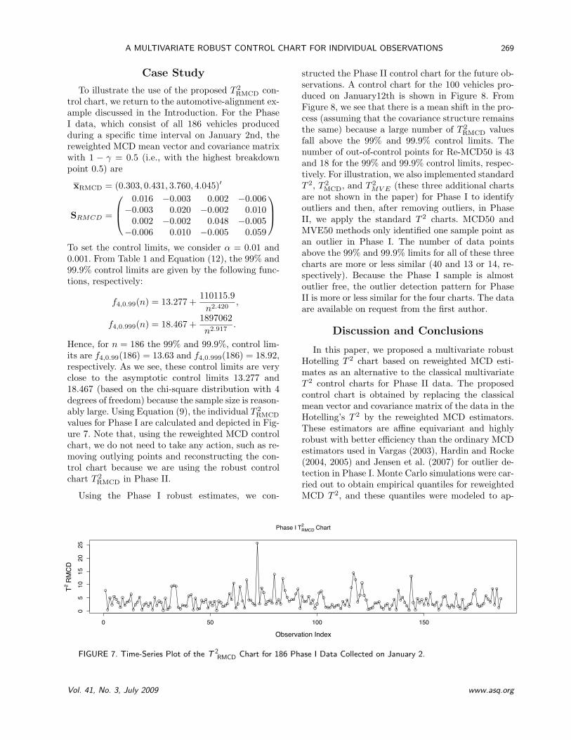
Case Study

To illustrate the use of the proposed T 2RMCD con-

trol chart, we return to the automotive-alignment ex-ample discussed in the Introduction. For the PhaseI data, which consist of all 186 vehicles producedduring a specific time interval on January 2nd, thereweighted MCD mean vector and covariance matrixwith 1 − γ = 0.5 (i.e., with the highest breakdownpoint 0.5) are

xRMCD = (0.303, 0.431, 3.760, 4.045)′

SRMCD =

⎛⎜⎝0.016 −0.003 0.002 −0.006

−0.003 0.020 −0.002 0.0100.002 −0.002 0.048 −0.005

−0.006 0.010 −0.005 0.059

⎞⎟⎠To set the control limits, we consider α = 0.01 and0.001. From Table 1 and Equation (12), the 99% and99.9% control limits are given by the following func-tions, respectively:

f4,0.99(n) = 13.277 +110115.9n2.420

,

f4,0.999(n) = 18.467 +1897062n2.917

.

Hence, for n = 186 the 99% and 99.9%, control lim-its are f4,0.99(186) = 13.63 and f4,0.999(186) = 18.92,respectively. As we see, these control limits are veryclose to the asymptotic control limits 13.277 and18.467 (based on the chi-square distribution with 4degrees of freedom) because the sample size is reason-ably large. Using Equation (9), the individual T 2

RMCD

values for Phase I are calculated and depicted in Fig-ure 7. Note that, using the reweighted MCD controlchart, we do not need to take any action, such as re-moving outlying points and reconstructing the con-trol chart because we are using the robust controlchart T 2

RMCD in Phase II.

Using the Phase I robust estimates, we con-

structed the Phase II control chart for the future ob-servations. A control chart for the 100 vehicles pro-duced on January12th is shown in Figure 8. FromFigure 8, we see that there is a mean shift in the pro-cess (assuming that the covariance structure remainsthe same) because a large number of T 2

RMCD valuesfall above the 99% and 99.9% control limits. Thenumber of out-of-control points for Re-MCD50 is 43and 18 for the 99% and 99.9% control limits, respec-tively. For illustration, we also implemented standardT 2, T 2

MCD, and T 2MV E (these three additional charts

are not shown in the paper) for Phase I to identifyoutliers and then, after removing outliers, in PhaseII, we apply the standard T 2 charts. MCD50 andMVE50 methods only identified one sample point asan outlier in Phase I. The number of data pointsabove the 99% and 99.9% limits for all of these threecharts are more or less similar (40 and 13 or 14, re-spectively). Because the Phase I sample is almostoutlier free, the outlier detection pattern for PhaseII is more or less similar for the four charts. The dataare available on request from the first author.

Discussion and Conclusions

In this paper, we proposed a multivariate robustHotelling T 2 chart based on reweighted MCD esti-mates as an alternative to the classical multivariateT 2 control charts for Phase II data. The proposedcontrol chart is obtained by replacing the classicalmean vector and covariance matrix of the data in theHotelling’s T 2 by the reweighted MCD estimators.These estimators are affine equivariant and highlyrobust with better efficiency than the ordinary MCDestimators used in Vargas (2003), Hardin and Rocke(2004, 2005) and Jensen et al. (2007) for outlier de-tection in Phase I. Monte Carlo simulations were car-ried out to obtain empirical quantiles for reweightedMCD T 2, and these quantiles were modeled to ap-

FIGURE 7. Time-Series Plot of the T 2RMCD Chart for 186 Phase I Data Collected on January 2.

Vol. 41, No. 3, July 2009 www.asq.org

270 SHOJA’EDDIN CHENOURI, ASOKAN MULAYATH VARIYATH, AND STEFAN H. STEINER

FIGURE 8. The T 2RMCD Chart for 100 Phase II Observations Collected on January 12. The dashed and solid horizontal

lines represent control limits based on 99.9% and 99% quantiles, respectively.

proximate control limits for any sample size. Oursimulation studies showed that the proposed robustcontrol charts (T 2

RMCD) are similar to standard T 2

charts in performance when the process is in-controland are more efficient than standard T 2 charts (withand without outlier removal in Phase I) when thereare outliers in the process during Phase I. We illus-trated our proposed method using a case study fromthe automotive industry.

Acknowledgments

The authors would like to thank the editor andtwo anonymous referees for their valuable comments,which substantially improved the overall presenta-tion of an earlier version of the paper. The work ofDrs. Chenouri and Steiner was partially supportedby the Natural Sciences and Engineering ResearchCouncil of Canada.

References

Butler, R. W.; Davies, P. L.; and Juhn, M. (1993). “Asymp-totics for the Minimum Covariance Determinant Estimator”.The Annals of Statistics 21, pp. 1385–1400.

Croux, C. and Haesbroeck, G. (1999). “Influence Func-tion and Efficiency of the Minimum Covariance DeterminantScatter Matrix Estimator”. Journal of Multivariate Analysis71, pp. 161–190.

Davies, P. L. (1987). “Asymptotic Behavior of S-Estimates ofMultivariate Location Parameters and Dispersion Matrices”.The Annals of Statistics 15, pp. 1269–1292.

Davies, P. L. (1992). “The Asymptotics of Rousseeuw’s Mini-mum Volume Ellipsoid Estimator”. The Annals of Statistics20, pp. 1828–1843.

Donoho, D. L. (1982). “Breakdown Properties of Multivari-ate Location Estimators”. Ph.D. Qualifying Paper, HarvardUniversity.

Donoho, D. L. and Huber, P. J. (1983). “The Notion ofBreakdown Point”. In A Festschrift for Erich L. Lehmannin Honor of His Sixty-Fifth Birthday, P. J. Bickel, K. A.

Doksum, and J. L. Hodges, Jr., eds., pp. 157–184. Belmont,CA: Wadsworth.

Gnanadesikan, R. and Kettenring, J. R. (1972). “RobustEstimates, Residuals, and Outlier Detection with Multire-sponse Data”. Biometrics 28, pp. 81–124.

Hardin, J. and Rocke, D. M. (2004). “Outlier Detection inthe Multiple Cluster Setting Using the Minimum CovarianceDeterminant Estimator”. Computational Statistics & DataAnalysis 44, pp. 625–638.

Hardin, J. and Rocke, D. M. (2005). “The Distribution ofRobust Distances”. Journal of Computational and GraphicalStatistics 14, pp. 928–946.

Hawkins, D. M. and Olive, D. J. (1999). “Improved Fea-sible Solution Algorithm for High Breakdown Estimation”.Computational Statistics and Data Analysis 30, pp. 1–11.

Hotelling, H. (1947). In Techniques of Statistical Analysis,C. Eisenhart, H. Hastay, and W. A. Wallis, eds., pp. 111–184.New York, NY: McGraw-Hill.

Huber, P. J. (1981). Robust Statistics. New York, NY: JohnWiley and Sons.

Jensen, W. A.; Birch, J. B.; and Woodall, W. H. (2007).“High Breakdown Estimation Methods for Phase I Multi-variate Control Charts”. Quality and Reliability EngineeringInternational 23(5), pp. 615–629.

Lopuhaa, H. P. (1989). “On the Relation Between S-Estimators and M-Estimators of Multivariate Location andCovariance. The Annals of Statistics 17, pp. 1662–1683.

Lopuhaa, H. P. (1999). “Asymptotics of Reweighted Estima-tors of Multivariate Location and Scatter”. The Annals ofStatistics 27, pp. 1638–1665.

Lopuhaa, H. P. and Rousseeuw, P. J. (1991). “BreakdownPoints of Affine Equivariant Estimators of Multivariate Lo-cation and Covariance Matrices”. The Annals of Statistics19, pp. 229–248.

Maronna, R. A. (1976). “Robust M-Estimators of Multivari-ate Location and Scatter”. The Annals of Statistics 4, pp.51–67.

Pison, G.; Van Alest, S.; and Willems, G. (2002). “SmallSample Corrections for LTS and MCD”. Metrika 55, pp. 111–123.

Rousseeuw, P. J. (1985). “Multivariate Estimation with HighBreakdown Point”. In Mathematical Statistics and Applica-tions, Section B, W. Grossmann, G. Pflug, I. Vincze, andW. Werz, eds., pp 283–297. Dordrecht: Reidel.

Journal of Quality Technology Vol. 41, No. 3, July 2009

A MULTIVARIATE ROBUST CONTROL CHART FOR INDIVIDUAL OBSERVATIONS 271

Rousseeuw, P. J. and Leroy, A. M. (1987). Robust Regres-sion and Outlier Detection. New York, NY: John Wiley andSons.

Rousseeuw, P. J. and Van Driessen, K. (1999). “A FastAlgorithm for the Minimum Covariance Determinant Esti-mator”. Technometrics 41, pp. 212–223.

Rousseeuw, P. J. and Yohai, V. (1984). “Robust Regressionby Means of S-Estimators”. In Robust and Nonlinear TimeSeries Analysis. Lecture Notes in Statistics 26, pp. 256–272.Berlin: Springer.

Rousseeuw, P. J. and van Zomeren, B. C. (1990). “Unmask-ing Multivariate Outliers and Leverage Points”. Journal ofAmerican Statistical Association 85, pp. 633–639.

Seber, G. A. F. (1984). Multivariate Observations. New York,NY: John Wiley and Sons.

Serfling, R. (1980). Approximation Theorems of Mathemat-ical Statistics. New York, NY: John Wiley and Sons.

Stahel, W. A. (1981).“ Robust Estimation: Infinitesimal Op-timality and Covariance Matrix Estimators”. Ph.D. Disser-tation, ETH, Zurich (in German).

Sullivan, J. H. and Woodall, W. H. (1996). “A Comparison

of Multivariate Control Charts for Individual Observations.Journal of Quality Technology 28, pp. 398–408.

Sullivan, J. H. and Woodall, W. H. (1998). “Adapting Con-trol Charts for the Preliminary Analysis of Multivariate Ob-servations”. Communications in Statistics, Simulation andComputation 27, pp. 953–979.

Tracy, N. D.; Young, J. C.; and Mason, R. L. (1992). “Mul-tivariate Control Charts for Individual Observations. Jour-nal of Quality Technology 24, pp. 88–95.

Vargas, J. A. (2003). “Robust Estimation in MultivariateControl Charts for Individual Observations”. Journal ofQuality Technology 35, pp. 367–376.

Wilks, S. S. (1962). Mathematical Statistics. New York, NY:John Wiley and Sons.

Willems, G.; Pison, G.; Rousseeuw, P. J.; and Van Alest,

S. (2002). “A Robust Hotelling Test”. Metrika 55, pp. 125–138.

Woodruff, D. L. and Rocke, D. M. (1994). “ComputableRobust Estimation of Multivariate Location and Shape inHigh Dimension Using Compound Estimators. Journal ofAmerican Statistical Association 89, pp. 888-896.

∼

Vol. 41, No. 3, July 2009 www.asq.org