A Multivariate Spatial Model for Soil Water Profiles

Stephan R. Sain,1 Shrikant Jagtap,2 Linda Mearns,3 and Doug Nychka4

July 20, 2004

SUMMARY: Pedotransfer functions are classes of models used to estimate soil water

holding characteristics based on commonly measured soil composition data as well as other

soil characteristics. These models are important on their own but are particularly useful

in modelling agricultural crop yields across a region where only soil composition is known.

In this paper, an additive, multivariate spatial process model is introduced that offers the

flexibility to capture the complex structure typical of the relationship between soil compo-

sition and water holding characteristics. A new form of pedotransfer function is developed

that models the entire soil water profile. Further, the uncertainty in the soil water charac-

teristics is quantified in a manner to simulate ensembles of soil water profiles. Using this

capability, a small study is conducted with the CERES maize crop model to examine the

sources of variation in the yields of maize. Here it is shown that the interannual variability

of weather is a more significant source of variation in crop yield than the uncertainty in

the pedotransfer function for specific soil textures.

KEY WORDS: Additive and mixed models, smoothing, pedotransfer functions, crop mod-

els.

1Geophysical Statistics Project, National Center of Atmospheric Research and Department ofMathematics, University of Colorado at Denver, P.O. Box 173364, Denver, CO 80217-3364,ssain@math.cudenver.edu. Corresponding author.

2Department of Agricultural and Biological Engineering, University of Florida3Environmental and Societal Impacts Group, National Center for Atmospheric Research4Geophysical Statistics Project, National Center for Atmospheric Research

1

1 Introduction

Soil scientists have long been interested in pedotransfer functions that are used to estimate

soil water holding characteristics from commonly measured soil composition data. These

water holding characteristics are necessary, along with other inputs such as weather, for use

with crop models such as the Crop Environment Resources Synthesis (CERES) models that

predict yields of maize, wheat, etc. Although crop yields are of interest in their own right,

our interest is in using these models to assess the impacts of the interannual variability

in climate as well as climate change. Crop yields are a useful integration of the weather

during a growing season and provide a meaningful summary measure of the meteorology at

a specific location. Considering the difference in the average yields predicted by the crop

models under weather simulated from present and a possible future climate is a metric

for climate change with agricultural and economic import. However, the uncertainty and

variation in the predicted yields are also of vital concern to scientists, researchers, and policy

makers. In particular, it is important to quantify how variation in the soil characteristics

influence the crop models. Understanding the uncertainty in the soil characteristics as well

as other inputs to the crop models will further our understanding of the uncertainty in the

predicted crop yields and the impact of climate change.

1.1 Soil Characteristics

The water holding characteristics of a soil are generally characterized by measurements

of the drained upper limit (DUL) and wilting point or lower limit (LL). It is these water

holding characteristics that are inputs for the CERES crop model. The DUL is defined as

the amount of water that a particular soil can hold after drainage is virtually complete.

The LL is defined as the smallest amount of water that plants can extract from a particular

soil. These values are often measured at different depths at a single location, yielding an

entire profile of water holding characteristics.

The direct measurement of DUL and LL is difficult and is only available for a limited

number of soils. In order to apply the crop model to a wide variety of soils, it is necessary

2

to infer DUL and LL from more commonly measured soil characteristics based on soil

composition and it is these measurements of the percentages of clay, sand, and silt that

are key components of most pedotransfer functions. Other variables are also at times

incorporated into pedotransfer functions. These include, for example, bulk density (the

weight of dry soil per unit volume of soil) and the amount of organic carbon in the soil.

1.2 Modeling Approaches for Pedotransfer Functions

A number of different approaches to the development of pedotransfer functions have ap-

peared in the literature. Multiple regression, nonlinear regression (e.g. neural networks),

and nonparametric methods such as nearest-neighbor regression have been used along with

methods based on established physical relationships and differential equations. Several re-

views have appeared in the literature discussing the various forms of pedotransfer functions

including Rawls et al. (1991), Timlin et al. (1996), Minasny et al. (1999), Pachepsky et

al. (1999), and Gijsman et al. (2002). However, there are still issues in applying modern

statistical models to this problem and, just as important, in characterizing the uncertainty

of the estimated pedotransfer function.

1.3 Impacts for Soil and Statistical Science

We propose a flexible procedure based on an additive, multivariate spatial process model

that simultaneously models the entire soil water profile of LL and DUL yielding a new and

innovative form of pedotransfer function. While accounting for the spatial dependence in

the LL and DUL as a function of depth, this model also allows for smooth contributions of

important covariates related to the soil composition as well as the inclusion of additional

covariates.

These types of models are complex and direct estimation of parameter values through,

for example, maximum likelihood or restricted maximum likelihood (REML) can be prob-

lematic. Beyond the specific contributions of such models in the development of new forms

of pedotransfer functions, we also introduce an iterative approach for fitting such mod-

3

els. Inspired by traditional approaches to geostatistics and algorithms like backfitting and

expectation-maximization (EM), it is demonstrated in this situation that our approach

produces parameter values consistent with those obtained via REML but with substantial

computational savings.

Although these models can be complicated, the additive structure of the model allows

the uncertainty in the predicted LL and DUL to be easily characterized. Further, the model

gives a framework for generating random realizations of soil water profiles for particular

collections of soil composition characteristics. These realizations can be interpreted as

random samples from the posterior distribution of the soil water profiles given the database

of observed soil water profiles. Of course, the variation in these random samples reflects

the uncertainty in the soil water profiles and the subsequent use as inputs to a crop model

will produce variation in crop yields.

1.4 Outline

The following section gives details about the data used in this work and Section 3 outlines

the construction of the model as well as estimation. Section 4 presents the results of the

model fitting and Section 5 presents a discussion of the prediction error in the model and

the generation of soil water profiles. Finally, Section 6 discusses an application utilizing the

CERES maize crop model to examine the behavior of the predicted crop yields for different

soil types.

2 Soil Data

The soil database used in this work consists of 272 individual measurements on 63 soil

samples selected by Gijsman et al. (2002) from a national field study of Ratliff et al. (1983)

and Ritchie et al. (1987). See also Jagtap et al. (2003). To our knowledge, this is one of

the most extensive soil databases for use in the development and validation of pedotransfer

functions.

Individual measurements from the original study that were beyond the reach of the

4

CLAY

SILTSAND

−2 0 2 4

−1.

0−

0.5

0.0

0.5

1.0

1.5

2.0

log(SAND/CLAY)

log(

SIL

T/C

LAY

)

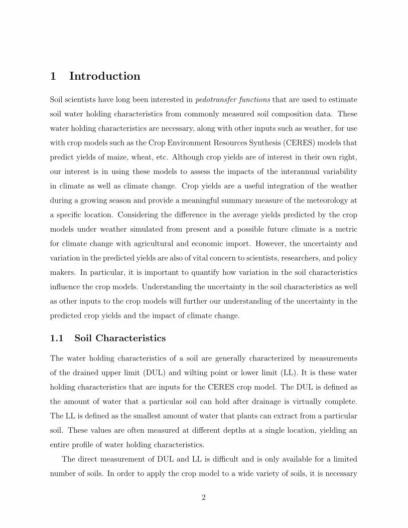
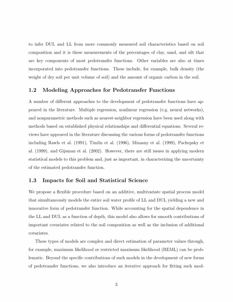
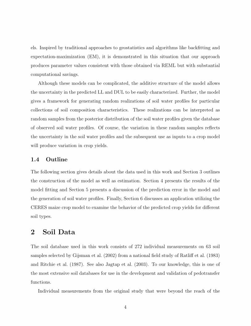
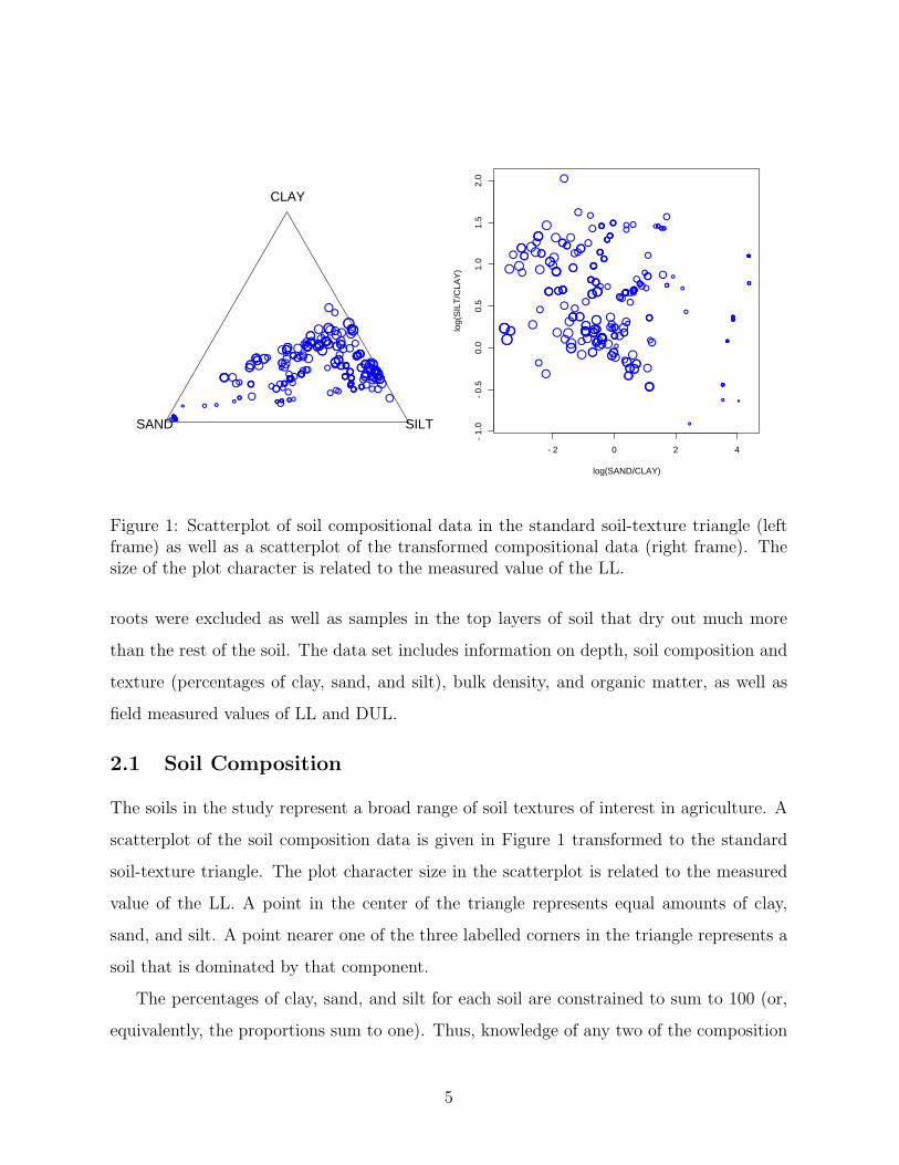
Figure 1: Scatterplot of soil compositional data in the standard soil-texture triangle (leftframe) as well as a scatterplot of the transformed compositional data (right frame). Thesize of the plot character is related to the measured value of the LL.

roots were excluded as well as samples in the top layers of soil that dry out much more

than the rest of the soil. The data set includes information on depth, soil composition and

texture (percentages of clay, sand, and silt), bulk density, and organic matter, as well as

field measured values of LL and DUL.

2.1 Soil Composition

The soils in the study represent a broad range of soil textures of interest in agriculture. A

scatterplot of the soil composition data is given in Figure 1 transformed to the standard

soil-texture triangle. The plot character size in the scatterplot is related to the measured

value of the LL. A point in the center of the triangle represents equal amounts of clay,

sand, and silt. A point nearer one of the three labelled corners in the triangle represents a

soil that is dominated by that component.

The percentages of clay, sand, and silt for each soil are constrained to sum to 100 (or,

equivalently, the proportions sum to one). Thus, knowledge of any two of the composition

5

percentages completely defines the third. So there are not three distinct variables in the

soil composition, rather the measurements inhabit a lower-dimensional structure. Aitchison

(1987) suggests transforming such data using the additive log-ratio transform. Consider

constructing two new variables defined as

X1 = log

(Silt

Clay

)X2 = log

(Sand

Clay

).

A scatterplot of X1 and X2 is also shown in Figure 1. The choice of which variable to use

in the denominator is somewhat arbitrary, and, for these data, the clay component is used

since that choice yields the smallest correlation among the transformed variables X1 and

X2.

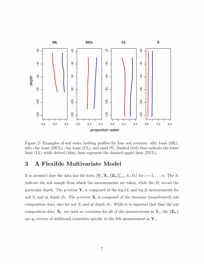
2.2 Soil Water Profiles

The data exhibit a nested structure in that each of the 63 different soil samples have

measurements of soil composition, LL, DUL, etc. taken at different depths. For a particular

soil, this collection of LL and DUL measurements at different depths make up the soil water

profile. Examples of the LL and DUL profiles for four particular soil texture types are

displayed in Figure 2. The soil texture classification is based on the relative percentages of

clay, sand, and silt. The data set includes soils with the following soil textures: silty loam

(SIL), silty clay loam (SICL), loam (L), clay loam (CL), sand (S), silty clay (SIC), sandy

loam (SL), sandy clay loam (SCL), clay (C) and loamy sand (LS).

As is shown by Figure 2, the LL and DUL measurements are constrained in the sense

that 0 < LL < DUL < 1. Since DUL is typically much less than 1, this suggests the

transformation

Y1 = log(LL) Y2 = log(∆)

where ∆ = DUL − LL. Given the measurements, the statistical problem now is to accu-

rately reproduce the profile structure in the Y1 and Y2 as a function of depth and across

the range of possible soil compositions and texture classes.

6

0.0 0.2 0.4

−12

0−

100

−80

−60

−40

−20

SIL

0.0 0.2 0.4

−12

0−

100

−80

−60

−40

−20

SICL

0.0 0.2 0.4

−12

0−

100

−80

−60

−40

−20

CL

0.0 0.2 0.4

−12

0−

100

−80

−60

−40

−20

S

proportion water

dept

h

Figure 2: Examples of soil water holding profiles for four soil textures: silty loam (SIL),silty clay loam (SICL), clay loam (CL), and sand (S). Dashed (red) lines indicate the lowerlimit (LL) while dotted (blue) lines represent the drained upper limit (DUL).

3 A Flexible Multivariate Model

It is assumed that the data has the form (Yi,Xi, Zkipk=1, Si, Di) for i = 1, . . . , n. The Si

indicate the soil sample from which the measurements are taken, while the Di record the

particular depth. The p-vector Yi is composed of the log LL and log ∆ measurements for

soil Si and at depth Di. The q-vector Xi is composed of the bivariate (transformed) soil

composition data, also for soil Si and at depth Di. While it is expected that that the soil

composition data, Xi, are used as covariates for all of the measurements in Yi, the Zki

are qk-vectors of additional covariates specific to the kth measurement in Yi.

7

3.1 Multivariate Regression Models

Construct the n×p matrix Y = [Y1 . . .Yn]′ and the n×q matrix X = [X1 . . .Xn]′, and, for

the moment, ignore the nested structure of the data, depth, and the additional covariates

Zki. The traditional approach to multivariate response regression suggests a model of

the form

Y = Xβ + ε (1)

where β is a q × p matrix of regression coefficients and ε = [ε1 . . . εn]′ is a n × p matrix

of errors. The standard assumptions on the error terms posit that, for each i = 1, . . . , n,

E[εi] = 0 and Var[εi] = Σ. Also, the rows of ε are assumed to be independent. Then the

least-squares estimates of β are equivalent to performing p individual regressions on the

columns of Y.

A second formulation of the multivariate response regression model in (1) can be con-

structed by stacking the columns of Y, yielding

vecY = (Ip ⊗X)vecβ + vecε, (2)

where vecY is now a np × 1 vector given by

vecY = [Y11 · · ·Y1nY21 · · ·Y2n]′ ,

and Y1i and Y2i represent the measurements of log LL and log ∆, respectively. Also, ⊗ is

the Kronecker product, vecβ is a qp×1 vector of regression coefficients, and vecε is a np×1

vector of errors. This formulation changes the behavior of the error structure somewhat.

For example, although E[vecε] = 0, Var[vecε] = Σ ⊗ In. In the following, we will drop

the vec notation and simply consider, for example, Y as a np × 1 vector while retaining

the knowledge that the first n elements of Y refer to the first response variable, that the

second set of n elements refer to the second response variable, etc.

3.2 An Extended Multivariate Model

Preliminary analysis as well as a close examination of the data in Figure 2 suggest that a

model such as those in (1) and (2) is inappropriate. These models fail because the response

8

is not linear and the covariance structure does not follow the simple Kronecker form. We

seek to generalize these simple models in several ways. First, through a type of additive

model, flexibility will be incorporated into the regression function, in particular, to model

the relationship between the transformed soil composition data and the transformed soil

water variables. Secondly, additional covariates, including those specific to just LL and ∆

will be included. Finally, there is a certain smoothness in the profiles in Figure 2 suggesting

that the measurements are correlated with depth. Hence, the model should be able to

account for dependence not only within measurements for each observation (e.g. between

LL and ∆ at the same depth for a particular soil) but also possible spatial dependence

between the observations (e.g. across LL and ∆ measurements at different depths for a

particular soil).

Consider expanding the multivariate response regression model as

Yi = P (Xi, Zkipk=1) + h(Xi) + εSi

(Di), (3)

where P is a fixed polynomial function, h is a random function of the transformed soil

composition, and εSiis a random error process accounting for both the variation between

measurements for a particular soil at some fixed depth and the spatial dependence across

measurements for a particular soil at different depths. The inclusion of h in the model is

equivalent to a form of nonparametric regression.

Assuming that the errors have a normal distribution, the model in (3) implies that Y

is multivariate normal with

E[Y] = Tβ Var[Y] = Σh + Σε. (4)

The regression matrix T is a block diagonal matrix with p blocks. The kth diagonal block

has the form [1 X Zk]. Here, 1 is a n-vector of 1’s (intercept), X is the n × q matrix

of variables common to all response variables and Zk is the n × qk matrix of explanatory

variables specific to the kth response variable. This structure implies that T and β have

p + nq +∑

k qk columns and elements, respectively.

9

3.3 Covariance Structures

The covariance matrix Σh in (4) is associated with random process h in (3) while Σε is the

covariance associated with the error process, εS. These covariance matrices have the form

Σh = diag(ρ1, . . . , ρp) ⊗K Σε = W ⊗B, (5)

where diag indicates a diagonal matrix. We assume that h is a stationary process and so

the matrix K contains elements of the form Kij = Cov[h(Xi), h(Xj)] = C(||Xi −Xj||) for

i, j = 1, . . . , n. A flexible class of covariance functions is the Matern family (Stein, 1999)

given by

C(d) = σ2 2(θd/2)νKν(θd)

Γ(ν)(6)

where d = ||Xi − Xj||, σ2 is a scale parameter, θ represents the range, ν controls the

smoothness, and Kν is a modified Bessel function of order ν. We use this family for mod-

elling the regression function relating soil parameters to composition. In this application,

the covariance function for K is fixed with σ2 = 1 (the parameters ρi adjust for different

variances), ν = 1, and θ is taken to be on the order of the range of the data.

The matrices W and B represent the within observation covariance (fixed depth) and

the across observation covariance (across depths), respectively. The p × p matrix W has

elements wij = Cov[εki, εkj] for all k = 1, . . . , n and i, j = 1, . . . , p. The matrix B is a n×n

matrix whose structure is more complex as it reflects the nested structure in the data,

i.e. the effect that measurements within a particular soil water profile are related across

depth. The elements of B are given by

bij =

Cov[εik, εjk] = C(||Di −Dj||) Si = Sj

0 otherwise,

for all k = 1, . . . , p and i, j = 1, . . . , n where again we assume that the process modelling

dependence on depth is stationary. The covariance function used here is the exponential

covariance given by

C(d) = exp(−(d/θ)2), (7)

10

where d = ||Di −Dj||. Note that that the exponential covariance function is in the Matern

family where ν = 0.5. Typically, the observations will be grouped by soil sample, indicated

by the Si. Hence, B will have a block diagonal structure and all of the off-diagonal elements

will be zero reflecting the independence of measurements from different soil samples.

Our choices for fixed and free parameters in the covariance functions is an attempt

to balance model flexibility with the amount of information available in the data. The

covariance function for h has only the scale parameters free to be estimated from the data,

while the covariance function for εS has both the scale parameters as well as the range

parameters free. This difference in the parameterization of the two covariance matrices is

due to important distinctions between the roles of the two random terms in the model and

the structure of the data used for estimation. As mentioned earlier, h is included in the

model as a form of nonparametric regression. Just as the bandwidth is more important

than the functional form of the kernel for optimal kernel smoothing (Scott, 1992, and Wand

and Jones, 1994), the scale parameter (or the ratio of the scale parameter to the range in

the case of an exponential covariance function) plays a similar role for optimal prediction

with kriging (Stein, 1999). With a single realization of the soil compositional data, it is

difficult to estimate both scale and range parameters for h. On the other hand, the nested

structure of the soil data is essentially comparable to multiple realizations which should

greatly improve our ability to estimate both sets of parameters for the covariance of εS. In

this case, different soil profiles are combined to yield information about the correlation of

water holding capacity with depth.

3.4 Smoothing

Smoothing the data to estimate the surface represented by h is accomplished by finding the

appropriate balance between the respective components of the overall covariance matrix.

However, it is also desirable to allow different amounts of smoothing across the different

variables. Formally, the full covariance matrix can be written as

Σh + Σε = diag(ρ1, . . . , ρp) ⊗K + W ⊗B

11

= w11 [diag(η1, . . . , ηp) ⊗K + V ⊗B]

= w11Ω, (8)

where ηi = ρi/w11 and the elements of V are of the form vij = wij/w11. Assuming that V,

B, and K are known, then smoothing can be accomplished by choosing the appropriate

values of η1, . . . , ηp. Larger values of ηi leads to rougher estimates.

3.5 Estimation I: REML

Given covariances for h and εS in (3), a standard estimator is the best linear unbiased

method (commonly known as universal kriging) which has the form

Y = Tβ + (diag(η1, . . . , ηp) ⊗K)δ. (9)

More traditional geostatistical methods for parameter estimation and prediction often use

the data twice. First, spatial covariance parameters are estimated by, for example, fitting

covariance models to sample covariance functions. Then, the data are used for prediction

at locations where data are not observed. See, for example, Cressie (1991). However, it is

difficult to fit covariance models in this fashion with fixed-effects terms present.

An alternative is to estimate model parameters using REML (Kitanidis, 1997; Stein,

1999; see also Wahba, 1990a, and Nychka, 2000). To demonstrate, take the QR decompo-

sition of T, i.e. write T as

T = [Q1 Q2]

[R0

],

where the matrix R is upper-triangular and Q = [Q1 Q2] is an orthogonal matrix with

Q1 having columns that span the column space of T and Q2 having columns that span

the space orthogonal to T. Then Q′2Y has zero mean and covariance matrix given by

Q′2(Σh + Σε)Q2. Hence, the likelihood corresponding to the transformed Q′

2Y only in-

volves covariance parameters, which in this case includes ρi, W, and θ from (7). The

likelihood is complex and closed form solutions for the parameter estimates are intractable.

12

However, the likelihood can be maximized via numerical methods. Then, given the covari-

ance parameters, estimates of β and predictions for δ are obtained directly as

β = (T′Ω−1

T)−1T′Ω−1

Y

δ = Ω−1

(Y −Tβ),

where Ω is an estimate of Ω in (8). Note that the form β is equivalent to the general-

ized least-squares estimator and that δ is equivalent to the best linear unbiased predictor

(BLUP).

3.6 Estimation II: An Iterative Approach

In practice, the size and complexity of data sets may lead to computational difficulties

when directly maximizing the likelihood. To counter such problems, we propose an iterative

approach to parameter estimation that is inspired by traditional approaches to geostatistical

data analysis as well as such procedures as backfitting (Breiman and Friedman, 1985;

Buja et al., 1989) and the expectation-maximization algorithm (Dempster et al., 1977).

The procedure cycles between a REML step to update the smoothing parameters, an

estimation/prediction step to update β and δ, and a final step examining residuals to

update estimates of W and B. We conjecture that, at convergence, the algorithm produces

approximate likelihood estimators that are comparable to those obtained from the REML.

The algorithm is as follows:

0. Initialize: Compute K and set W = Ip and B = In.

1. Using a modified form of the REML discussed Section 3.5, estimate η1, . . . , ηp. Be-

cause the matrices K, W, and B are fixed at this stage, profiling the log-likelihood

with respect to w11 from (8) leaves the log-likelihood as a function of only the

η1, . . . , ηp. Estimates of the ηi are then found through a simple grid search.

2. Estimate β and predict δ via

β = (T′Ω−1

T)−1T′Ω−1

Y

13

δ = Ω−1

(Y −Tβ).

3. Compute residuals as R = Y − Y where Y is given in (9).

a. Update W (B fixed).

b. Update B (W fixed).

4. Repeat steps 1-3 until parameter estimates converge.

Some remarks on the third step in the procedure are in order. Residuals are computed

by subtracting estimates of the fixed effects and predictions of the random effects. To

justify the use of such residuals to estimate the covariance matrix of the error process (W

and B), let Y = µ + h + ε denote a general mixed effects model. Then, assuming h and ε

are independent Gaussian random variables, the conditional distribution of Y−µ−h given

h is a zero mean Gaussian with the covariance matrix of ε. See, for example, McCulloch

and Searle (2000).

Considering the updating of W and B, note that the log-likelihood associated with the

residuals R is proportional to

−n

2|W| − p

2|B| −R′(W−1 ⊗B−1)R (10)

where the determinant and inverse of Σε follow directly from the properties of Kronecker

products and R = [r′1 · · · r′p]′ with ri denoting the n-vector of residuals for the ith variable.

Note that the quadratic form in (10) can be rewritten as

tr(W−1n∑

i=1

n∑j=1

bijuju′i)

where tr indicates the trace of a matrix, bij is the ijth element of B−1 and ui indicates the

p-vector of residuals for the ith observation constructed by unstacking the residual vector,

R, into a n × p matrix. Thus, an update of W can be obtained via

W =1

n

n∑i=1

n∑j=1

bijuju′i

=1

nU′B−1U

14

η1 η2 W11 W22 W12 θREML 5.84 1.66 0.0765 0.0483 -0.0222 134.6

Iterative 5.74 2.21 0.0697 0.0445 -0.0217 144.2

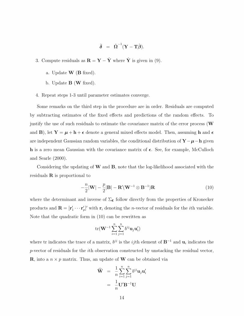
Table 1: A comparison of parameter estimates from REML (Section 3.5) and the iterativeapproach (Section 3.6).

where U indicates the n × p matrix of (unstacked) residuals. See, for example, Theorem

4.2.1 from Mardia et al. (1979).

Unfortunately, there is no easy update for B. However, B is simply a function of the

range θ from (7), and, given W, (10) can be computed easily and maximized via a simple

grid search.

4 Results

The methods presented in Section 3 were used to fit the model in (3) and (9). The matrix

X contains the transformed composition data, which are common to both log LL and log ∆.

A measure of organic matter in the soil was included as an additional covariate for log LL

(Zi1, i = 1, . . . , n). Also, the profiles in Figure 2 suggest that ∆ is smaller for deeper soils.

Hence, both linear and quadratic terms were included as additional covariates for log ∆ by

setting Zi2 = [(Di − 70) (Di − 70)2]′ for i = 1, . . . , n where the midpoint of the values

of depth in the data is 70. Approximately ten iterations of the algorithm in Section 3.6

were required for fitting the model and convergence was monitored by examining parameter

estimates and predicted values.

Table 4 shows a comparison of the parameter estimates of the covariance matrices

obtained from directly maximizing the likelihood using REML and the iterative algorithm

from Section 3.6. The parameter estimates are quite close and yield virtually identical

predictions of log LL and log ∆.

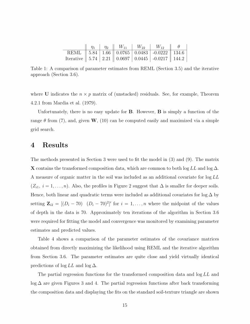
The partial regression functions for the transformed composition data and log LL and

log ∆ are given Figures 3 and 4. The partial regression functions after back transforming

the composition data and displaying the fits on the standard soil-texture triangle are shown

15

−2 0 2 4

−1.

0−

0.5

0.0

0.5

1.0

1.5

2.0

−4.

5−

4.0

−3.

5−

3.0

−2.

5−

2.0

−1.

5

X1

X2

Y

Figure 3: The partial regression function for log LL as a function of the transformed com-position data.

−2 0 2 4

−1.

0−

0.5

0.0

0.5

1.0

1.5

2.0

−3.

0−

2.8

−2.

6−

2.4

−2.

2−

2.0

−1.

8

X1

X2

Y

Figure 4: The partial regression function for log ∆ as a function of the transformed com-position data.

16

−4.

5−

4.0

−3.

5−

3.0

−2.

5−

2.0

−1.

5

CLAY

SILTSAND

−3.

0−

2.8

−2.

6−

2.4

−2.

2−

2.0

−1.

8

CLAY

SILTSAND

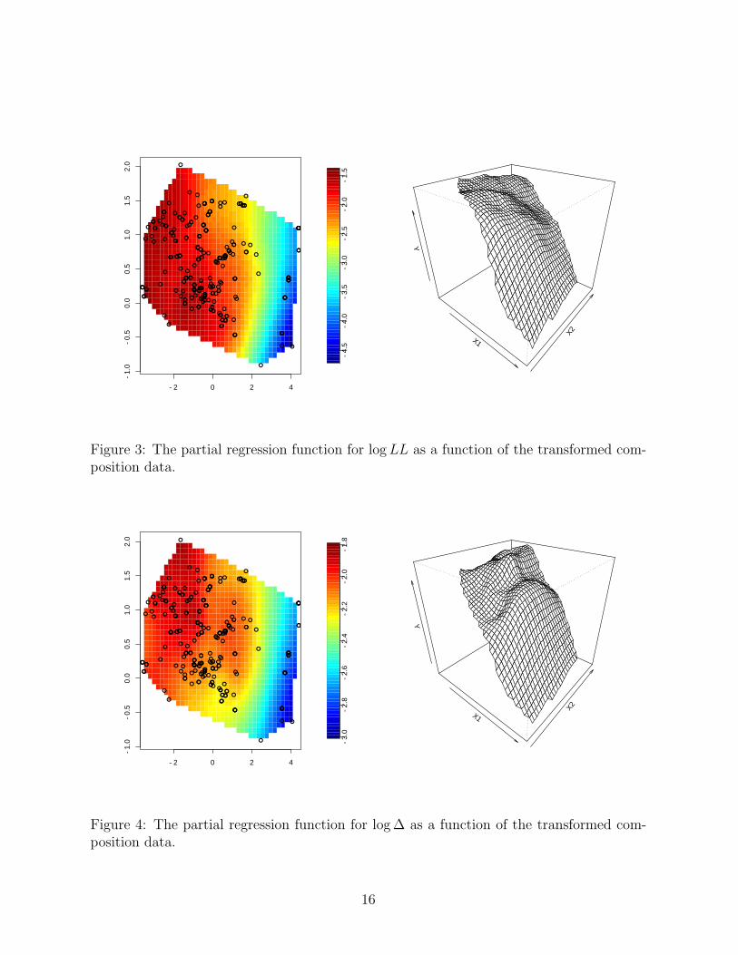
Figure 5: Partial regression functions for log LL (left frame) and log ∆ (right frame) as afunction of the transformed composition data after transforming back to the soil composi-tion triangle.

in Figure 5. In general, the fits show considerable structure with smaller log LL and log ∆

for larger values of X1 = log(Silt/Clay), increasing log LL and log ∆ as X1 decreases, and

a levelling out of log LL and log ∆ for larger X2 = log(Sand/Clay) values.

This phenomenon translates into sandy soils having the lowest log LL and soils with a

stronger clay component having the highest log LL. Sandy soils also had lower log ∆ values,

suggesting that the LL and DUL are closer together. Interesting, the final regression fits

for log ∆ seem to peak and plateau near more loamy soils. These results indicate that the

random component h plays a significant role in determining the composition beyond just

a simple polynomial relationship.

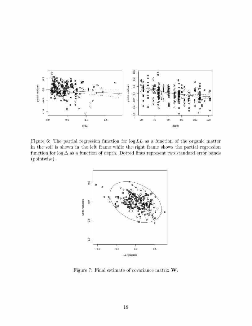
The contribution of organic matter to the log LL is shown in the left frame of Figure

6 along with two standard error bands (pointwise). There does not seem to be strong

evidence of a significant contribution of organic carbon to log LL. The contribution of

depth to the log ∆ is shown in the right frame of Figure 6, also with two standard error

bands (pointwise). Depth, on the other hand, does seem to have a significant impact on

17

0.0 0.5 1.0 1.5

−1.

0−

0.5

0.0

0.5

orgC

part

ial r

esid

uals

20 40 60 80 100 120

−0.

6−

0.4

−0.

20.

00.

20.

40.

6

depthpa

rtia

l res

idua

ls

Figure 6: The partial regression function for log LL as a function of the organic matterin the soil is shown in the left frame while the right frame shows the partial regressionfunction for log ∆ as a function of depth. Dotted lines represent two standard error bands(pointwise).

−1.0 −0.5 0.0 0.5

−1.

0−

0.5

0.0

0.5

LL residuals

Del

ta r

esid

uals

Figure 7: Final estimate of covariance matrix W.

18

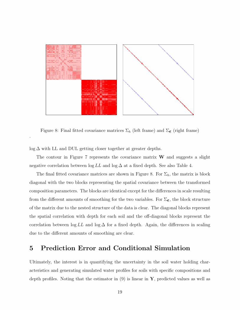
Figure 8: Final fitted covariance matrices Σh (left frame) and Σε (right frame).

log ∆ with LL and DUL getting closer together at greater depths.

The contour in Figure 7 represents the covariance matrix W and suggests a slight

negative correlation between log LL and log ∆ at a fixed depth. See also Table 4.

The final fitted covariance matrices are shown in Figure 8. For Σh, the matrix is block

diagonal with the two blocks representing the spatial covariance between the transformed

composition parameters. The blocks are identical except for the differences in scale resulting

from the different amounts of smoothing for the two variables. For Σε, the block structure

of the matrix due to the nested structure of the data is clear. The diagonal blocks represent

the spatial correlation with depth for each soil and the off-diagonal blocks represent the

correlation between log LL and log ∆ for a fixed depth. Again, the differences in scaling

due to the different amounts of smoothing are clear.

5 Prediction Error and Conditional Simulation

Ultimately, the interest is in quantifying the uncertainty in the soil water holding char-

acteristics and generating simulated water profiles for soils with specific compositions and

depth profiles. Noting that the estimator in (9) is linear in Y, predicted values as well as

19

the prediction error are easily found. Let (X0i, Z0kipk=1, S0i, D0i) for i = 1, . . . , n0 denote

the data structure for a new soil where predictions of the water holding characteristics are

desired. Further, let X0 denote the n0 × q matrix of explanatory variables common to all

the response variables and Z0k the n0× qk matrix of explanatory variables specific to the

kth response variable. Predicted values are obtained via

Y0 = T0β + K0δ

= A0Y (11)

where the matrix T0 is given by

T0 =

[1 X0 Z01 0

0 1 X0 Z02

],

K0 is a n0×n matrix with elements Kij = C(||X0i−Xj||) and C is the covariance function

defined in (6). Letting

M = (T′Ω−1

T)−1T′Ω−1

,

then

A0 = T0M + K0Ω−1

(I−M).

The prediction error is obtained via

Var(Y0 − Y0) = Var(Y0 −A0Y)

= Var(Y0) + A0Var(Y)A′0 − 2A0Cov(Y,Y0). (12)

The variance of Y is easily estimated by plugging in the parameter estimates for Σh and

Σε. Similarly, an estimate for the variance of Y0 can also be easily constructed. The

covariance between Y and Y0 is implied by the random function h in (3) and is obtained

via the covariance function based on the transformed compositional data.

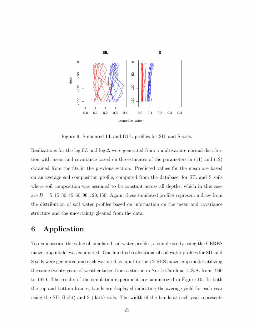
Figure 9 shows ten simulated LL and DUL profiles for two soils of interest, silty loam

(SIL) and sand (S) based on the estimates obtained from the multivariate spatial model.

20

0.0 0.1 0.2 0.3 0.4

−15

0−

100

−50

0

SIL

0.0 0.1 0.2 0.3 0.4

−15

0−

100

−50

0

S

proportion water

dept

h

Figure 9: Simulated LL and DUL profiles for SIL and S soils.

Realizations for the log LL and log ∆ were generated from a multivariate normal distribu-

tion with mean and covariance based on the estimates of the parameters in (11) and (12)

obtained from the fits in the previous section. Predicted values for the mean are based

on an average soil composition profile, computed from the database, for SIL and S soils

where soil composition was assumed to be constant across all depths, which in this case

are D = 5, 15, 30, 45, 60, 90, 120, 150. Again, these simulated profiles represent a draw from

the distribution of soil water profiles based on information on the mean and covariance

structure and the uncertainty gleaned from the data.

6 Application

To demonstrate the value of simulated soil water profiles, a simple study using the CERES

maize crop model was conducted. One hundred realizations of soil water profiles for SIL and

S soils were generated and each was used as input to the CERES maize crop model utilizing

the same twenty years of weather taken from a station in North Carolina, U.S.A. from 1960

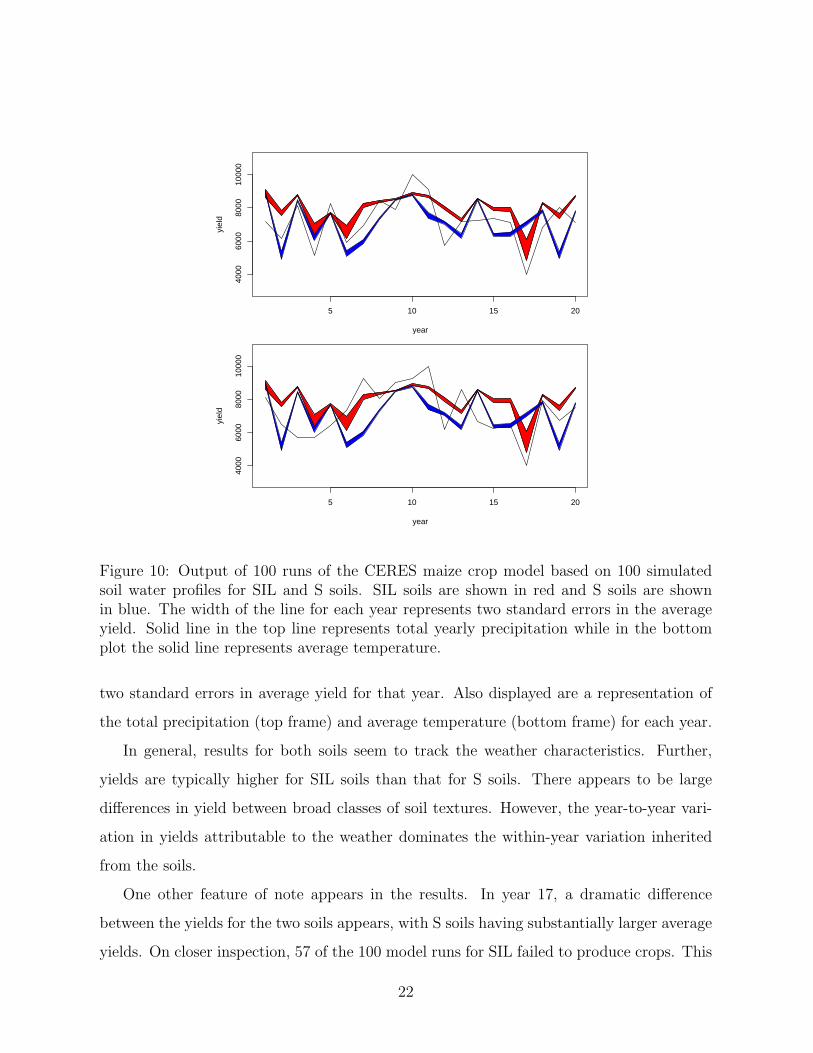
to 1979. The results of the simulation experiment are summarized in Figure 10. In both

the top and bottom frames, bands are displayed indicating the average yield for each year

using the SIL (light) and S (dark) soils. The width of the bands at each year represents

21

5 10 15 20

4000

6000

8000

1000

0

year

yiel

d

5 10 15 20

4000

6000

8000

1000

0

year

yiel

d

Figure 10: Output of 100 runs of the CERES maize crop model based on 100 simulatedsoil water profiles for SIL and S soils. SIL soils are shown in red and S soils are shownin blue. The width of the line for each year represents two standard errors in the averageyield. Solid line in the top line represents total yearly precipitation while in the bottomplot the solid line represents average temperature.

two standard errors in average yield for that year. Also displayed are a representation of

the total precipitation (top frame) and average temperature (bottom frame) for each year.

In general, results for both soils seem to track the weather characteristics. Further,

yields are typically higher for SIL soils than that for S soils. There appears to be large

differences in yield between broad classes of soil textures. However, the year-to-year vari-

ation in yields attributable to the weather dominates the within-year variation inherited

from the soils.

One other feature of note appears in the results. In year 17, a dramatic difference

between the yields for the two soils appears, with S soils having substantially larger average

yields. On closer inspection, 57 of the 100 model runs for SIL failed to produce crops. This

22

year is characterized by low temperatures and low precipitation. Because the SIL requires

a greater amount of water in the soil (refer to Figures 2 and 9), the lack of precipitation

leads to decreases in yields and more frequent failed crops.

7 Concluding Remarks

An additive, multivariate regression model is introduced that includes smooth contributions

of the explanatory variables common to all of the response variables as well as traditional

linear contributions of additional covariates specific to each response variable. It should

be noted that variations on this basic structure are easily accommodated. The model is

also able to account for complex error structures, including spatial and other forms of

dependence.

The model presented here shares a connection with thin-plate smoothing splines (de

Boor, 1978; Wahba, 1990a; and Green and Silverman, 1994) and spatial models including

universal kriging (Cressie, 1991). This model also offers an alternative to the semiparamet-

ric smoothing approach of Ruppert et al. (2003). On the surface, these regression techniques

are quite different and are motivated from different perspectives. However, there has been

much effort on establishing the clear connection between the spline smoothing and spatial

models (Wahba, 1990b; Cressie, 1990; Kent and Mardia, 1994; and Nychka, 2000). This

connection lies in the additive structure of these models that includes fixed, polynomial

components as well as random components whose correlation structure effectively controls

the amount of smoothing.

The model parameters can be fit using established techniques such as REML. How-

ever, for complex data structures and regression functions this may be impractical and

an iterative procedure is introduced to reduce the computational burden. In this setting,

parameter estimates very similar to those obtained from REML are obtained using the

iterative approach. While we believe this algorithm is effective at producing reasonable

parameter estimates, more study is certainly warranted.

The model is used to develop a new type of pedotransfer function for estimating soil

23

water holding characteristics based on soil composition data as well as other covariates.

This model is unique in that the entire soil water profile as a function of depth is estimated.

Of perhaps more importance is that the model offers the ability to capture the uncertainty

in the soil characteristics as well as the ability to simulate complete soil water profiles.

Using this model, a small simulation study was conducted in which soil water profiles

were simulated for two soil texture classes and yields computed using the CERES maize

crop model. This initial study suggests that there are differences in yields between soil

texture classes (based on composition), but that variation in yields due to the variation

in weather dominate that due to variation in soils and uncertainty in the pedotransfer

function.

Finally, this work represents a preliminary result that is a part of a larger collabora-

tion between statisticians and scientists who are studying global climate change by using

statistical models to assess the sources of uncertainly in large, complicated and typically

deterministic models used to describe natural phenomenon.

Acknowledgements

This research is supported in part by the National Science Foundation under grant DMS

9815344.

24

References

Breiman, L. and Friedman, J.H. (1985), “Estimating optimal transformations for multiple

regression and correlations (with discussion),” Journal of the American Statistical

Association, 80, 580-619.

Buja, A., Hastie, T.J., and Tibshirani, R.J. (1989), “Linear smoothers and additive models

(with discussion),” Annals of Statistics, 17, 453-555.

Cressie, N.A.C. (1990), Reply to Wahba’s letter, American Statistician, 44, 256-258.

Cressie, N.A.C. (1991), Statistics for Spatial Data, New York: John Wiley.

de Boor, C. (1978), A Practical Guide to Splines, New York: Springer-Verlag.

Dempster, A.P., Laird, N.M., and Rubin, D.B. (1977), “Maximum likelihood from incom-

plete data via the EM algorithm (with discussion)”, Journal of the Royal Statistical

Society, Ser. B, 39, 1-37.

Gijsman, A.J., Jagtap, S.S., and Jones, J.W. (2002), “Wading through a swamp of com-

plete confusion: how to choose a method for estimating soil water retention parame-

ters for crop models,” European Journal of Agronomy, 18, 75-105.

Green, P.J. and Silverman, B.W. (1994), Nonparametric Regression and Generalized Lin-

ear Models: a Roughness Penalty Approach, London: Chapman and Hall.

Kent, J.T. and Mardia, K.V. (1994), “The link between Kriging and thin plate spline

splines,” In Kelly, F.P. (ed.), Probability, Statistics, and Optimization, New York:

John Wiley.

Kitandidis, P.K. (1997), Introduction to Geostatistics: Applications in Hydrogeology, Cam-

bridge University Press.

Jagtap, S.S., Lall, U., Jones, J.W., Gijsman, A.J., and Ritchie, J.T. (2003), “A dynamic

nearest neighbor method for estimating soil water parameters,” In press.

25

McCulloch, C.E. and Searle, S.R. (2000), Generalized, Linear, and Mixed Models, New

York: John Wiley.

Mardia, K.V., Kent, J.T., and Bibby, J.M. (1979), Multivariate Analysis, London: Aca-

demic Press.

Minansy, B., McBratney, A.B., and Bristow, K.L. (1999), “Comparison of different ap-

proaches to the development of peodtransfer functions for water retention curves,”

Geoderma 93, 225-253.

Nychka, D.W. (2000), “Spatial-process estimates as smoothers,” In Schimek, M.G. (ed.),

Smoothing and Regression: Approaches, Computation, and Application, New York:

John Wiley.

Pachepsky, Y.A., Rawls, W.J., and Timlin, D.J. (1999), “The current status of pedo-

transfer functions: their accuracy, reliability and utility in field- and region-scale

modeling,” In Corwin, D.L., Loague, K.M., and Ellsworth, T.R. (ed.), Assessment

of Non-Point Source Pollution in the Vadose Zone, Geophysical Monograph 108,

American Geophysical Union, Washington, D.C.

Ratliff, L.F., Ritchie, J.T., and Cassel, D.K. (1983), “Field-measured limits of soil water

availability as related to laboratory-measured properties,” Soil Science Society of

America Journal, 47, 770-775.

Rawls, W.J., Gish, T.J., and Brakensiek, D.L. (1991), “Estimating soil water retention

from soil physical properties and characteristics,” Advances in Agronomy, 16, 213-

234.

Ritchie, J.T., Ratliff, L.F., and Cassel, D.K. (1987), “Soil laboratory data, field descrip-

tions and filed measured soil water limits for some soils of the United States,” ARS

Technical Bulletin, ARS Agriculture Research Service and Soil Conservation Service

/ Stat Agriculture Experimental Stations, Temple, Texas.

26

Ruppert, D., Wand, M.P., and Carroll, R.J. (2003), Semiparametric Regression, Cam-

bridge, U.K.: Cambridge University Press.

Scott, D.W. (1992), Multivariate Density Estimation: Theory, Practice, and Visualization,

New York: John Wiley.

Stein, M.L. (1999), Interpolation of Spatial Data: Some Theory for Kriging, New York:

Springer-Verlag.

Timlin, D.J., Pachepsky, Y.A., Acock. B., and Whisler, F. (1996), “Indirect estimation

of soil hydraulic properties to predict soybean yield using GLYCIM,” Agricultural

Systems, 52, 331-353.

Wahba, G. (1990a), Spline Models for Observational Data, Philadelphia: SIAM.

Wahba, G. (1990b), Letter to the editor, American Statistician, 44, 256.

Wand, M.P. and Jones, M.C. (1995), Kernel Smoothing, London: Chapman and Hall.

27