39 5 , ru e W ell ing ton O t ta w a ON K1A 0N 4 C a n a d a
NOTICE:The author has granted a nonexclusive license allowing Library and Archives Canada to reproduce, publish, archive, preserve, conserve, communicate to the public by telecommunication or on the Internet, loan, distribute and sell theses worldwide, for commercial or noncommercial purposes, in microform, paper, electronic and/or any other formats.
AVIS:L'auteur a accorde une licence non exclusive permettant a la Bibliotheque et Archives Canada de reproduire, publier, archiver, sauvegarder, conserver, transmettre au public par telecommunication ou par I'lnternet, preter, distribuer et vendre des theses partout dans le monde, a des fins commerciales ou autres, sur support microforme, papier, electronique et/ou autres formats.
The author retains copyright ownership and moral rights in this thesis. Neither the thesis nor substantial extracts from it may be printed or otherwise reproduced without the author's permission.
L'auteur conserve la propriete du droit d'auteur et des droits moraux qui protege cette these.Ni la these ni des extraits substantiels de celle-ci ne doivent etre imprimes ou autrement reproduits sans son autorisation.
In compliance with the Canadian Privacy Act some supporting forms may have been removed from this thesis.
While these forms may be included in the document page count, their removal does not represent any loss of content from the thesis.
Conformement a la loi canadienne sur la protection de la vie privee, quelques formulaires secondaires ont ete enleves de cette these.
Bien que ces formulaires aient inclus dans la pagination, il n'y aura aucun contenu manquant.
i * i
CanadaR ep ro d u ced with p erm issio n o f th e copyrigh t ow n er. Further reproduction prohibited w ithout p erm ission .
ABSTRACT
The thesis describes the development and implementation o f the basic concept o f
a Virtual Dressing Room (VDR) simulation, which is a system to allow customers to use
their own 3D models to ‘try on’ outfits and see how they look before they buy them. The
primary objective o f the project is to design a multilayer perceptron neural network for
the virtual dressing room.
This project was divided into three main tasks: (1) theory o f creation o f the 3D
model, (2) design and implementation o f a multilayer perceptron neural network, and (3)
implementation o f the VDR system user interface. This thesis project is mainly focused
on designing the neural network. The multilayer perceptron neural network is designed
to retrieve a particular preference o f garments for a specific customer depending on his or
her age, gender and the ethnicity. Thus, the customer does not have to go through the
entire database o f the garments to select one piece o f clothes based on his or her interest.
The database will contain all sorts o f clothes: wedding dresses for females and suits for
males, sports wears for both genders, night gowns, and they might also have unique
dresses that are o f interest to specific cultures such as Sarees for South Asians, etc. For
example, a customer from Africa will not waste his or her time by going through the
entire database to choose one for his or her preference. The multilayer perceptron neural
network will choose the dresses for their specific interest. The neural network is trained
for each ethnic group, but if someone comes with multiple ethnic backgrounds such as
African American, the neural network will generalize the preference o f the garments for
them too.
ii
R ep ro d u ced with p erm issio n o f th e copyrigh t ow n er. Further reproduction prohibited w ithout p erm ission .
ACKNOWLEDGEMENT
I would like to express my sincere thanks to my supervisors Professors Peter Liu
and Brahim Chebbi for their support, patience and well-anchored guidance throughout
the process o f this thesis.
I would also like to express my very special thanks to my parents, and to my
brother and sister. Without their support and encouragement, this work would not have
been possible.
R ep ro d u ced with p erm issio n o f th e copyrigh t ow n er. Further reproduction prohibited w ithout p erm ission .
APPENDIX A - THE RESULTED IMAGES.......................... 88
R ep ro d u ced with p erm issio n o f th e copyrigh t ow n er. Further reproduction prohibited w ithout p erm ission .
VI
LIST OF TABLES
Table 1: Input bit for gender............................................................................................................58
Table 2: Input bits for age group....................................................................................................58
Table 3: Input bits for ethnic group............................................................................................... 59
Table 4: Iteration Table for Standard B P......................................................................................66
Table 5: Inputs and Outputs from Standard BP Algorithm......................................................66
Table 6: Iteration Table for Modified-LABP...............................................................................67
Table 7: Inputs and Outputs from Modified-LABP Algorithm...............................................68
Table 8: A set o f Sample Inputs and Desired Outputs...............................................................71
Table 9: A set o f Sample Inputs and Outputs from Standard BP Algorithm for VDR
system ...................................................................................................................................................72
Table 10: A set o f Sample Inputs and Outputs from Modified-LABP Algorithm for VDR
system ...................................................................................................................................................73
Table 11: A set o f Sample Inputs and Outputs from Modified-LABP Algorithm for VDR
system with 4 S ty les......................................................................................................................... 75
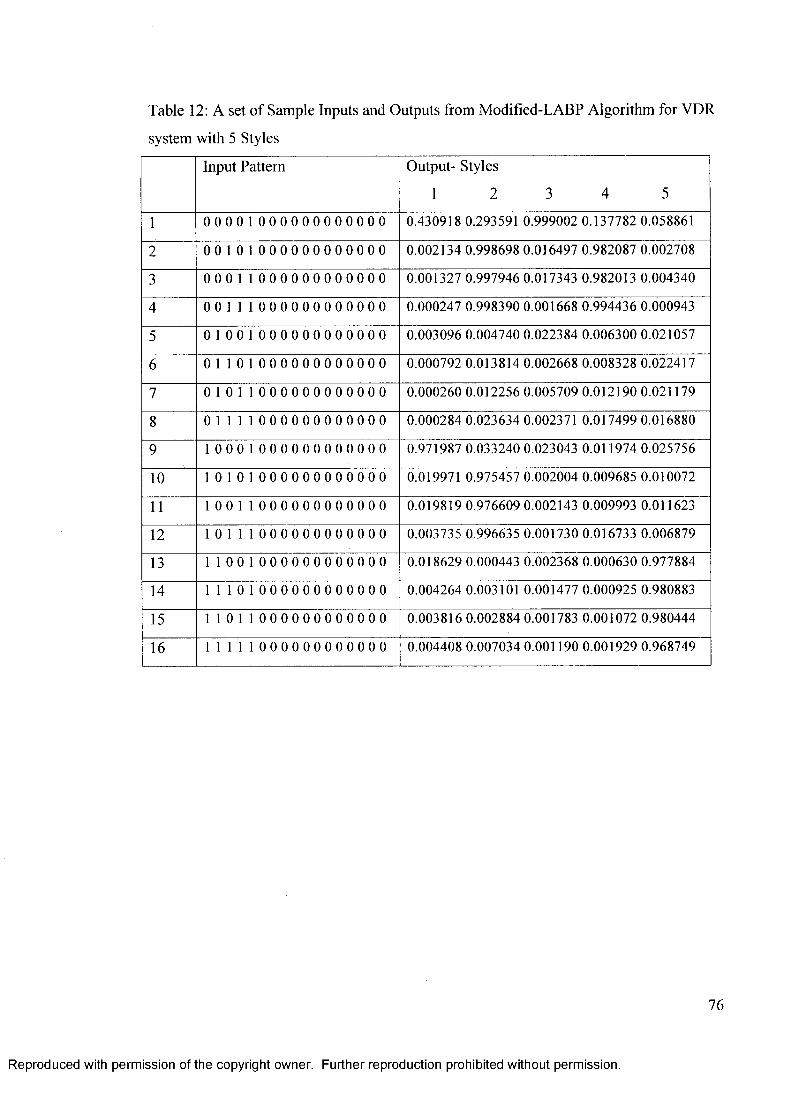
Table 12: A set o f Sample Inputs and Outputs from Modified-LABP Algorithm for VDR
system with 5 S ty les......................................................................................................................... 76
Table 13: A set o f Sample Inputs and Desired Outputs for 7 Styles..................................... 77
Table 14: A set o f Sample Inputs and Outputs from Modified-LABP Algorithm for VDR
system with 7 S ty les......................................................................................................................... 78
Table 15: A set o f Sample Inputs and Outputs from Modified-LABP Algorithm for VDR
system with 8 S ty les......................................................................................................................... 79
vii
R ep ro d u ced with p erm issio n o f th e copyrigh t ow n er. Further reproduction prohibited w ithout p erm ission .
Table 16: A Sample Generalization Result 80
vii i
R ep ro d u ced with p erm issio n o f th e copyrigh t ow n er. Further reproduction prohibited w ithout p erm ission .
LIST OF FIGURES
Figure 1: Overview o f 3D Model Reconstruction [1]................................................................ 10
Figure 2: Image with Extracted Features [1 ] ............................................................................... 13
Figure 3: Password User Interface................................................................................................. 43
Figure 4: Main YDR System User Interface...............................................................................44
Figure 5 : Help P age.......................................................................................................................... 46
Figure 6: Original Image and Filtered Im age..............................................................................50
Figure 7: Silhouette Images o f Front and Side V iew ................................................................. 53
Figure 8: 3D Reconstructed Images...............................................................................................55
Figure 9: Architecture o f the Neural Network.............................................................................57
Figure 10: Desired and Actual outputs with added Noise level...............................................74
Figure 11: Original and Gaussian and Salt and Pepper Noisy Im ages..................................88
R ep ro d u ced with p erm issio n o f th e copyrigh t ow n er. Further reproduction prohibited w ithout p erm ission .
x
CHAPTER 1 - INTRODUCTION
This thesis project proposes a Virtual Dressing Room (VDR) simulation to allow
clothing store customers to use their own 3D model to try the suitability o f outfits before
they buy them. The purpose o f this simulation is to improve the clothing stores’
customer friendliness. In clothing stores, the customers have to try on the garments every
time to select the one that they want. This will not allow the customer to try more than
perhaps 10 or 15 outfits due to the time limits o f patience or boredom. Moreover, the
customer can try only the materials that are available to them in the store they are
currently in. In order to avoid these two circumstances and to improve sales by allowing
customers to try more materials in a shorter time period, this project proposes a Virtual
Dressing Room (VDR) system. This will allow customers to try clothing on a computer
R ep ro d u ced with p erm issio n o f th e copyrigh t ow n er. Further reproduction prohibited w ithout p erm ission .
without physically wearing them and also to try on the clothes that are offered in other
branches o f the store without going there.
There will no longer be a need for individual changing rooms. A hall with a few
stations will fulfill the purpose o f the existing changing rooms. There will be two kinds
o f stations: one capable o f taking photos to create 3D images in the computer and the
other with a computer to try the clothes. Photo stations will each have 4 fixed cameras
and a place where the customer is required to stand when the photos are taken. Using
these photos, a 3D image o f the customer will be reconstructed. The 3D image can be
accessed by the user at the computer station using a password, which will be given to the
customer at the photo station. There are many methods to reconstruct 3D images. In this
report, a method is discussed and a modified version o f it is implemented for this project.
After the reconstruction o f the 3-D model, the user can select garments from the
database to try on the model. These images o f the garments can be anywhere in the
stores’ computer network. Distributed shared memory (DSM) is used to acquire these
images from remote nodes. Many methods are used in implementing DSM. In this
project, the analysis o f the five most popular methods has been used to draw a conclusion
o f the most efficient method.
After having the full 3-D human body model and images o f garments, there is a
need to display specific garments for a specific customer instead o f wasting their time by
requiring the customer to go through the entire database. For example, the preferences o f
the style o f a teenaged customer are different from those o f a middle-aged customer. In
2
R ep ro d u ced with p erm issio n o f th e copyrigh t ow n er. Further reproduction prohibited w ithout p erm ission .
addition to age differences, there will be gender, ethnic, shape and size differences. To
choose the specific garments for a specific customer, Multilayer Perceptron (MLP) neural
network is used. In this project, the neural network will be trained with age, gender and
ethnicity as inputs and preference o f styles o f the garments as outputs. Three methods are
discussed in this project: standard back propagation (BP), Lyapunov stability-based
adaptive back-propagation (LABP), and recursive least squares (RLS). Afterwards, the
standard BP and a new version o f LABP are implemented to test and prove that the
Modified-LABP gives a better performance for this project.
1.1 Motivation
One o f the difficult and time consuming aspects o f buying a garment is fitting the
garment on one individual and seeing the look o f the garment on him or her. Even if, a
customer likes them, he or she cannot try on all the garments physically. To pick one,
they have to choose some garments at first sight and then try on the few they picked.
What if the one garment that they ignored would be good on them? They will never
know that because they did not try that one.
Another difficult part is whether a particular garment is available in store or not.
If it is not in the store, a customer might have to travel to another branch or wait until it is
brought in from the warehouse. This is another problem which is time consuming and
troublesome.
3
R ep ro d u ced with p erm issio n o f th e copyrigh t ow n er. Further reproduction prohibited w ithout p erm ission .
These problems can be solved with a virtual dressing room (VDR) system. The
customer does not have to try on all the garments physically to see the fitting. However,
they can try all the garments in a virtual environment, if they want, because mouse
clicking is not going to take much o f their time. Moreover, the customer does not have to
travel from one branch to another to try out a garment. They can see all the garments that
can be purchased from all the branches o f the store by viewing through the VDR system.
This project also helps the clothing store managements by improving sale. If a
customer cannot find clothes in one store, he or she might not go to another branch o f the
same store. They might go to another store located in the neighbourhood. The VDR
system will prevent these inconveniences. Furthermore, an easy way to see the fitting o f
the garment will attract more customers to the store. Therefore, this will improve sales in
clothing stores. Also, stores would not need large showrooms to display their garments.
As the customers can see the garments on the computer, there would be no need for more
customer service personnel to help customers to locate garments or to put the garments
back on the shelf from the fitting room. This would reduce stores’ operating expenditure.
The time saving and conveniences are the main reasons for my motivation to propose the
VDR system.
The motivation for the neural network, which is the main contribution for this
VDR system, is to give an extra feature to the VDR system. In the clothing stores there
will be many kinds o f outfits: wedding dresses for women and suits for men, night
gowns, sports clothes, casual garments, party dresses, and so on. When a customer wants
4
R ep ro d u ced with p erm issio n o f th e copyrigh t ow n er. Further reproduction prohibited w ithout p erm ission .
to select a casual dress, he or she has to go through the entire database to select one dress.
By inputting personal information such as age, gender and ethnicity o f the customer
through the neural network, the customer’s preference o f the style o f garments will be
obtained. As such, customers would not have to go through the entire database to select
their clothes.
1.2 Contribution
Designing o f a neural network to obtain the preference o f customers based on
their gender, age and ethnicity is my contribution toward VDR system. The neural
network will get age, gender, and the ethnic background from the customer. The neural
network will be trained with many customers’ preferences. From the trained network, the
customer will be shown the clothes that suit his or her taste.
A survey is done on DSM systems to choose a better DSM to get the garments’
images from remote nodes. The remote access is important because each branch o f the
clothing store will have their separate servers with the garments that are available in that
particular branch. If a customer is not interested in any o f the clothing in that particular
branch, the VDR system will access the database form other branches o f the store. For
this process, a better DSM is needed for remote access.
R ep ro d u ced with p erm issio n o f th e copyrigh t ow n er. Further reproduction prohibited w ithout p erm ission .
1.3 Overview
In the following sections, a detailed analysis o f user interface o f VDR system, 3D
human model reconstruction, distributed shared memory (DSM), and Multilayer
Perceptron (MLP) Neural network are presented with implementations and results o f user
interface o f VDR system, 3D human model reconstruction and MLP Neural network.
Subsequently, the report presents a short discussion o f future work followed with the
conclusion.
R ep ro d u ced with p erm issio n o f th e copyrigh t ow n er. Further reproduction prohibited w ithout p erm ission .
6
CHAPTER 2 - BACKGROUND AND ANALYSIS
2.1 Introduction
A survey is done on 3D modeling, distributed memory system (DSM) and neural
network. The 3D modeling is to reconstruct a 3D model o f the customer and garments so
when a customer picks a dress from the database, it will be tried on his or her 3D model.
The DSM is to get all the garments from all servers from other branches o f the
stores. If there is only one server, there is a danger o f loosing the entire database o f
garments if there is a problem with a server. Further, overload o f system access can be
generated if many customers form many stores try to access the server at the same time.
7
R ep ro d u ced with p erm issio n o f th e copyrigh t ow n er. Further reproduction prohibited w ithout p erm ission .
Also, there will be customers who will be happy with the clothes from one store, so no
need for remote access at that time. Thus, there is a need for server in each store. If the
need o f remote access is aroused, the DSM can be used. For this purpose, there is a
survey done on DSM to choose the best DSM for this particular system. Last but not
least, the survey is done on neural networks to choose the better neural network for this
VDR system.
2.2 Human Model
A 3D human model is required for Virtual Dressing Room (VDR) system to try
garments without the person actually wearing it. There are many methods to reconstruct a
3D model image from photos. Two papers by [2] Cipolla and Giblin, and [3] Zhao and
Mohr proposed 3D image surface reconstruction using apparent contours. 3D image
quadric surface reconstruction is proposed by Cross and Zisserman [4], Conic surface
reconstruction for photo-grammetry techniques proposed Slama [5], Sullivan and Ponce
proposed silhouette with B-splines based reconstruction methods [6], Two papers [7], [8]
proposed the method, which deform a mesh model to fit the actual image o f the person.
Furthermore, the paper by Chang and Gerhard proposed free form surface reconstruction
[9]- [1] proposed the reconstruction o f 3D image using a humanoid model and four
orthogonal view images. The details o f this method are discussed in the following section
because the modification o f this method is used for this VDR system implementation.
8
R ep ro d u ced with p erm issio n o f th e copyrigh t ow n er. Further reproduction prohibited w ithout p erm ission .
2.2.1 3D Model Reconstruction Using Humanoid Model
To generate a 3-D human model o f a customer, a generic humanoid 3D model is
used [1], From this generic model four orthogonal views (front, back and both sides)
images are produced. These are already saved in the database. When a customer stands
on the landmark in front o f the camera four orthogonal view photos will be taken. These
images, called data images, will undergo filtering, edge detection and creation o f
silhouette images. After the creation o f silhouette images on both generic humanoid
model and data orthogonal view images, a set o f key feature points will be found on both
sets o f images. The feature points on the model and data images are aligned to match
both sets o f images. From these silhouette images, with the feature points, 2D-to-2D
linear affine mapping creates sets o f dense images [1], These dense 2D images are then
used to define the deformation for the 3D model [1], Using this deformation on the
humanoid 3D model, the 3D model o f an actual human body will be reconstructed. The
details o f each step is discussed in the following sub-sections. Figure 1 shows an
overview o f the algorithm: la is the humanoid model, lb is orthogonal images o f
humanoid model, lc is the orthogonal views o f a person, Id is the silhouette images o f
the humanoid model with features, le is the silhouette images o f the person with features,
I f is the dense images and lg is the 3D model [1].
R ep ro d u ced with p erm issio n o f th e copyrigh t ow n er. Further reproduction prohibited w ithout p erm ission .
(a) Cionorio mode l (b> M od e l proi tv i ion
I I 1 I 'I 11 I n 'U',
W ^ p ®
A m
f t& *
i c ; i a p l u i v d i n i . i j e .
■ e i ( a p l u i v d i m a g e da la >ilhi>uc-ue
^ ' 11 Deu ce 2d mapping o f data image e.n mode l si lhouei te
,-J M"f i - ■ ;;.\
U M$0 f||
( e i 31.) Model
Figure 1: Overview o f 3D Model Reconstruction [1]
In this section, reconstruction o f 3D model o f a human body will be discussed in
detail. The model is built using Matlab. The following sections will go through the
process in detail.
10
R ep ro d u ced with p erm issio n o f th e copyrigh t ow n er. Further reproduction prohibited w ithout p erm ission .
2.2.2 Humanoid Model
Any public available humanoid model can be used for this algorithm. This
humanoid model is a 3D polygonal mesh segment [1].
U J = ( 1)
Here UjNp is to represent the polygonal mesh with a list o f N p 3D vertices.
2.2.3 Image Capture
Using the cameras, all the four orthogonal view images are taken. This will give
a set o f four data images o f a customer.
I - , i = 1,2,3,4 (2)
R ep ro d u ced with p erm issio n o f th e copyrigh t ow n er. Further reproduction prohibited w ithout p erm ission .
11
The homogeneous coordinate o f the camera 3D to 2D projection is
u' = Ex' = ME,x (3)
where
u - (u,v,w)~ 3D point
it = (u / w,v / v i ' ) - 2D point in the camera image plane
5c' = (x,y,z , l ) - 3D point
5c - (x, y, z) - world homogenous coordinate
P is 4x3 projection matrix, which is changed into 3x4 camera calibration matrix M. Ej is
the extrinsic parameter o f view transformation.
where Rj is 3x3 rotation matrix and tj is 3x1 translation vector. 0 is 3x1 vector o f zeros. fu
and fv are camera calibration parameters (focal lengths) and ou and ov are image origin.
fu = vertical pixels x distance to camera vertical height
fv = horizontal pixels x distance to camerahorizontal height
/„ 0 o„ 0
M = 0 f v ov 0
0 0 1 0(4)
(5)
12
R ep ro d u ced with p erm issio n o f th e copyrigh t ow n er. Further reproduction prohibited w ithout p erm ission .
2.2.4 Feature Extraction
The key features need to be extracted in order to establish the correct
correspondence between humanoid orthogonal view images and data images. Figure 2
shows the front orthogonal view image with features [1],
(a) Image (b) Silhouette (c) Extrema (d) Features Figure 2: Image with Extracted Features [1]
An algorithm to find feature points is given as follows [1]. First, it explains about
finding the extrema points Uei-e5 as shown in figure 2c. To find the extrema points on the
top o f the head, the following formula is used,
uel = min[jw; j^ ' j and (6)
Ve, = V, (7)
The minimum is used here because the top o f the head is the contour point with
minimum vertical coordinate u.
13
R ep ro d u ced with p erm issio n o f th e copyrigh t ow n er. Further reproduction prohibited w ithout p erm ission .
To calculate the extrema points on the left arm, Ue2 and right arm, Ue5, the
following formula is used,
ve2 = min^vv ) and (8)
ue2 = Uj (9)
ve5 = m a x ({v jj) and (10)
uei = Uj (11)
Because the arms take as the minimum and maximum on horizontal coordinates
on the contour points, here the minimum and maximum o f horizontal coordinates, v, are
used.
To evaluate the centroid o f the silhouette image, the following equation is used
1 Npu = E «(i) (12)
c N 1=ip
To calculate the extrema points on the left feet, Ue3 and right feet, Ue4 , the
maximum vertical coordinate o f the contour on either side o f the centroid, vc, is used.
ue3 - max[{w; }jV'’J and (13)
V,3 = V, ^ Vc (14)
ueA = max({tty ) and (15)
ve4 = v , ^ v c (16)
14
R ep ro d u ced with p erm issio n o f th e copyrigh t ow n er. Further reproduction prohibited w ithout p erm ission .
After finding the extrema points, the algorithm went on and explained how to
extract the feature points shown in figure 2d. The feature points for crotch ufl, left arm
U(2 - and right arm u^ are evaluated with vertical coordinates, u.
Crotch U/]= min(jw; }^e3) and (17)
Left arm
Right arm
V/! =
un = min({M/ ) and
V/2 =V ,
un = min({w; }'^4) and
V/3 = V;
(18)
(19)
(20)
(21)
(22)
The feature points for left shoulder Uf4, and right shoulder Uf5 are evaluated with
horizontal coordinates, v.
Left shoulder
Right shoulder
74 = min(W-2-J andV/4 = V/2
m/ 5 = m i n ( { W /} ^ 5 ) a n d
V/J = v /3
(23)
(24)
(25)
(26)
15
R ep ro d u ced with p erm issio n o f th e copyrigh t ow n er. Further reproduction prohibited w ithout p erm ission .
2.2.5 2D to 2D Silhouette Mapping
After the feature point extraction, using these points, a dense image is created. As
it is mentioned in the feature points extraction the body parts can be separated into seven
parts: head, shoulder, left arm, right arm, torso, left feet and right feet. By a 2D linear
mapping, a body part can be created using the humanoid model and the data image.
u D = S u M (27)
Equation 27 coordinates a particular body part in the mapping, which is between the
corresponding silhouette images o f humanoid and data.
5 =s «
s.„Suv K
(28)
0 0 1
where s represents rotation, shear and scale; and t represents the translation. sv
represents the horizontal scaling factor and su represents the vertical scaling factor.
Because o f the principal axis o f the body parts are aligned, suv and svu are zero.
u° - u D_ max min O Q t
" ~ u M - u M ( }max min
t ——s uM + u Du u m in min (30)
16
R ep ro d u ced with p erm issio n o f th e copyrigh t ow n er. Further reproduction prohibited w ithout p erm ission .
(31)
t v(u) = - s v(u)v*m (u) + V°m (U) (32)
2.2.6 2D to 3D Silhouette Mapping
After 2D to 2D mapping, the next step is 2D to 3D mapping. For this affine
transform from orthogonal 2D to 3D model, the 3D displacement is required. For the
displacement component, first inverse projections must be calculated from the following
formula:
(33)
Where X,j represents the scaling factor.
fu
(34)/ v / ,
0 0 1
0 0 0
(35)
17
R ep ro d u ced with p erm issio n o f th e copyrigh t ow n er. Further reproduction prohibited w ithout p erm ission .
x D = x M + Ax, - Aj (x d )r ; ' M - ] [uf + A m , ) - RT% (36)
Using the above formula the 3D displacement component can be calculated as follows
Ax, * 2, (xM ) r ; ]M - ] (m ,m + A m , ) - R~% - x M (37)
When the estimated displacement component is put on the vertex on the 3D humanoid
mode it will give affine transform to orthogonal to 3D image.
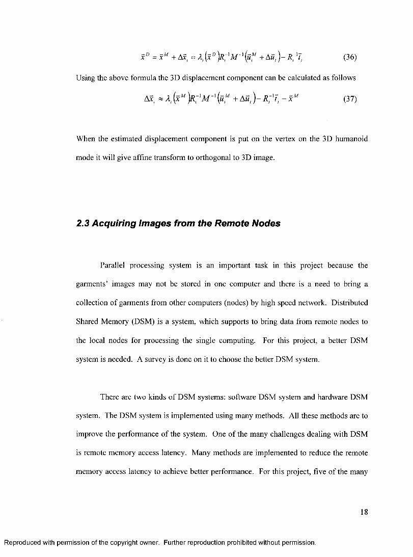
2.3 Acquiring Images from the Remote Nodes
Parallel processing system is an important task in this project because the
garments’ images may not be stored in one computer and there is a need to bring a
collection o f garments from other computers (nodes) by high speed network. Distributed
Shared Memory (DSM) is a system, which supports to bring data from remote nodes to
the local nodes for processing the single computing. For this project, a better DSM
system is needed. A survey is done on it to choose the better DSM system.
There are two kinds o f DSM systems: software DSM system and hardware DSM
system. The DSM system is implemented using many methods. All these methods are to
improve the performance o f the system. One o f the many challenges dealing with DSM
is remote memory access latency. Many methods are implemented to reduce the remote
memory access latency to achieve better performance. For this project, five o f the many
18
R ep ro d u ced with p erm issio n o f th e copyrigh t ow n er. Further reproduction prohibited w ithout p erm ission .
methods, which were proposed by many talented authors, are analyzed: maximized
speedup through performance prediction [10], hiding latency through bulk transfer [11],
improving performance with speculation [12], RAPID [13], and extended kernel mode
[14].
2.3.1 Maximized Speedup through Performance Prediction
The major interest o f implementing a parallel processing system is to improve the
performance. Normally, a lager DSM system gives better speed. However, because o f
the overhead cost for large size o f DSM system, the performance could not be improved
or even degraded. Therefore, the best performance can be achieved by determining the
appropriate size o f the DSM system [10],
In the paper, “Maximizing Speedup through Performance Prediction for
Distributed Shared Memory Systems,” a performance prediction model is proposed. A
DSM system Proteus is implemented. The runtime information was used to predict the
performance o f any parallel applications, which run on Proteus. Proteus DSM system
contains a set o f runtime Library to provide globally shared address space among nodes;
Ethernet connects the nodes. Proteus also supports dynamic node reconfiguration that
allows them to add or remove a new computer anytime; that is Proteus supports node
reconfiguration to adjust the system size at runtime. Proteus also supports per-node
multithreading, thread migration, synchronization primitives, and load balancing [10],
19
R ep ro d u ced with p erm issio n o f th e copyrigh t ow n er. Further reproduction prohibited w ithout p erm ission .
The prediction method was used to collect runtime information. Using this
runtime information, the execution time o f application was predicted under different
system sizes. The following equation was used to predict the time application,
t { n ) = — t (n) (38)n
t(n) is the predicted time o f application; ts is the time o f application executing in one
node; n is number o f nodes used for the execution; and tp0 is the time induced by
parallelizing overhead [10] and this tpo can be predicted by using following formula,
tp o M = K ys M + Korn M + K a i , M (39)
tcom is communication overhead; tsys is system overhead; and twait is waiting and load
balancing overhead. Using t(n), the predicted time o f application, the DSM size is
adjusted to appropriate size which gives the best performance [10],
By using this performance prediction mechanism, the appropriate system size,
which gives max speedup, is determined. The experiment result shows that the accuracy
of the performance prediction mechanism is acceptable [10].
R ep ro d u ced with p erm issio n o f th e copyrigh t ow n er. Further reproduction prohibited w ithout p erm ission .
2 0
2.3.2 Hiding Latency through Bulk Transfer and Prefetching
DSM machine achieves high performance by caching o f sharing data. This will
reduce the remote node usage, so the remote access latency will be reduced. But this
works fine and gives good performance only on fine-grain pattern. In coarse-grain
pattern, the performance is reduced by cache miss and remote access latency because
coarse-grain pattern has small size o f cache compare to shared memory in the system.
This limitation can be overcome by software prefetching; however, there are some
critical problems in this approach. One o f the problems is “memory latency widely
varies depending on the remote node in which the required data is located” [11].
To overcome these problems and to get good performance, a bulk transfer and
prefetching method is proposed in the paper, “Hiding Latency Through Bulk Transfer
and Prefetching in Distributed Shared Memory Multiprocessors.” First, the remote
access latency was overcome by converting remote access into local access. For this, a
part o f local memory was used as a destination o f the bulk transfer. The Adaptive
Granularity (AG) was used for bulk transfer. When a node requests data, the remote node
will send a bulk o f data; but, when false sharing expected, the remote node only sends
half o f the bulk data, which contains the requested data. If there is invalidation message,
it will only affect the half bulk. Therefore, the memory latency problem is solved
because the data is in local node. AG also guarantees the consistency o f the replication
data in local memory [11].
21
R ep ro d u ced with p erm issio n o f th e copyrigh t ow n er. Further reproduction prohibited w ithout p erm ission .
After the data is replicated and stored in local memory, software prefetching is
used to overcome the local access latency. This software prefetching is developed into
uni-processor; so, the frequently coherent traffic problem, which is caused by multi
processors specific characteristics, is overcome [11].
When this bulk transfer and prefetching method are simulated, the result shows
that the memory latency for local and remote access was reduced by 25-40% [11].
2.3.3 Improving the Performance with Speculation
DSM brings data, which is located in remote node to local node for processing.
DSM cache data from remote memory to local memory and runs coherent protocol to
ensure all replicas o f data remains coherent to improve the performance. Because o f high
overhead o f the coherent operation, software DSM performance is degraded [12],
In the paper, “Improving the Performance o f Software Distributed Shared
Memory with Speculation,” Speculation Home-based Release Consistency (SHRC)
method is proposed that uses speculation to improve the performance. Speculation is
executing an operation before it is actually needed. “Speculation can improve the
performance by weakening dependencies in program execution” [12]. Speculation
predicts the subordinate processing, which will be needed in the future use, and execute it
before the outcome is required. This speculation was used here to predict the remote
22
R ep ro d u ced with p erm issio n o f th e copyrigh t ow n er. Further reproduction prohibited w ithout p erm ission .
data, which will be required later. Then, a protocol was used to transfer the remote data
from the home node to the local node before the data is needed. This mechanism, which
uses speculation, is implemented in the home node (remote node) [12].
They modified Home-based Lazy Release Consistency (HLRC) protocol into
Speculation Home-based Release Consistency (SHRC), which is responsible for
maintaining and distributing the data store on the memory space to other nodes. This
protocol implies that it will only send the updated version o f the data to other nodes if
only they were asked. The extended version o f HLRC protocol, SHRC, will speculatively
perform certain coherence operation in the data before it is required.
This SHRC maintains a table with patterns o f past shared memory access. SHRC
protocol will use these patterns to predict the future memory access and transfer them to
the local mode. Therefore, local nodes will not try to access remote data from home
node. The home node itself sends the remote data to the local node, which may require
the data in future. Therefore, there will not be a remote access. It will always be local
access.
For the application, which has regular access pattern, this method performs
effectively and efficiently. The SHRC improves performance by reducing the remote
access latency.
23
R ep ro d u ced with p erm issio n o f th e copyrigh t ow n er. Further reproduction prohibited w ithout p erm ission .
2.3.4 RAPID
There are many methods that were proposed to reduce remote memory access
latency. In a large scale DSM, a node, which needs some data from a remote, will
broadcast messages to all nodes. The remote node which has the requested data will
send a message back to the node which requested the data with requested data “if the data
is clean,” or forward the request back ‘if the data is dirty.” This transfer undergoes
communication with remote nodes to access remote memory. Increase in remote memory
access latency is the main problem when the nodes on DSM system increase. The
methods, which were proposed to reduce the remote memory access latency, successfully
achieved the goal but they were expensive because most o f these methods require more
bandwidth [13].
In the paper, “RAPID: reconfigurable and scalable all-photonic interconnect for
distributed shared memory multiprocessors”, there is a method proposed to reduce the
remote memory access latency using fibre optical interconnects which provides higher
bandwidth and lower latency and lower cost [13].
This RAPID architecture design contains “3-tuples”: P, D and G. P is number o f
processors in a node (an assumption - only one processor is assigned to one node); D is
number o f nodes in a group; and G is number o f groups (D > G is another assumption to
ensure that every group communicates to every other group). There are two sub
networks: scalable intragroup interconnection (IGI) and scalable intergroup remote
24
R ep ro d u ced with p erm issio n o f th e copyrigh t ow n er. Further reproduction prohibited w ithout p erm ission .
interconnection (SIRI). All nodes are connected to these sub-networks through the
intergroup passive coupler (1GPC). The local and remote communications are separated
to ensure efficient implementation. All local interconnects are implemented using
waveguide optics and all remote interconnections are implemented using fibre optics
because fibre optics can be extended to different length [13].
Each node is identified as R(d,g), where the d is node number and g is the group
number. Within the group, all the nodes are connected to multiplexers and de
multiplexers. This will help for local and remote communication. The wavelength is
reused to design an efficient wavelength assignment strategy. For this strategy, the
spatial division multiplexing (DSM) technique is used [13].
Each node is assigned to a wavelength. When nodeO wants to communicate to
nodel within the same group (local communication), nodeO will use the wavelength; this
wavelength is assigned to nodel to transmit the data. Therefore, each node will receive
optical packet at the unique wavelength that is assigned to that node [13].
For remote communication, there are two groups involved: destination and source
group. For a specific destination, a source group is assigned to a unique wavelength at
which it can transmit the packet to destination group [13].
For message routing in RAPID, there are three possibilities: local message
routing, remote message routing and broadcast. If it is a local message routing, the
25
R ep ro d u ced with p erm issio n o f th e copyrigh t ow n er. Further reproduction prohibited w ithout p erm ission .
source and the destination nodes are in the same group, such as R (0, g l) and R (1, g l).
The source node uses the pre-assigned wavelength o f the destination node to transmit the
packet using waveguide optics. If it is a remote communication, the source and
destination nodes are not in the same group. The source node will use the specific
wavelength, which is assigned to the specific source group, to transmit packet using fibre
optics. The node in the destination that receives the packet will forward the packet to the
destination node using the wavelength o f the destination node. If it broadcasts and the
broadcasting is for only the nodes within the group, it will use wavelength 0 to transmit
the message. If it is broadcasting for all the groups, the source node uses the specific
wavelengths that for the destination group. A node in the destination group gets the
message and uses wavelength 0 to broadcast the message to the nodes within the specific
destination group [13].
This architecture is much faster and inexpensive and reduces the remote access
latency. RAPID maximizing the channel availability for communication and wavelength
are reused for local and remote communications. This RAPID architecture provides high
bandwidth and highly scalable network with minimized latency. If this achieved by
traditional electrical way, it will be much more expensive [13].
R ep ro d u ced with p erm issio n o f th e copyrigh t ow n er. Further reproduction prohibited w ithout p erm ission .
2 6
2.3.5 Extended Kernel Mode
Many people are interested in clusters o f personal computers. A set o f kernel
mechanism allows users to control the DSM on this cluster. These parallel applications
need processors and memory scalability; but the software DSM depends on the OS
virtual memory manager and do not maximize the usage o f the local memory for data
sharing. Moreover, the DSM uses mechanism to ensure data consistency at the expense
o f increasing system complexity. To solve these problems, memory is managed globally.
For this global memory management, first, OS virtual memory mechanism must be
extended. Then a set o f module must be provided for basic functionalities with minimum
overhead. Later, high-level modules will support the DSM protocols [14].
In this paper, “Distributed Shared Memory in Kernel Mode,” a new set o f kernel
mechanism is proposed to allow users to have full control on the DSM. This new set o f
kernel mechanism is called MOMEMTO (MOre MEMory Than Others) DSM system.
This MOMEMTO extends Linux 2.4 kernel and provides a set o f mechanism to support
global shared memory. MOMEMTO provides a basic shared mechanism by creating and
managing its own virtual memory area (VMA) in kernel. If a user requests memory
address, the MOMEMTO creates its own virtual memory address and uses them in
process’ VMA. Then the process uses this MOMEMTO memory. Each application has
virtual memory segment into its address space. Normally, a node will have its own
virtual memory segment. In MOMEMTO, all nodes will have their own virtual memory
segment. But all the nodes will share them. Therefore, the virtual memory segment is
27
R ep ro d u ced with p erm issio n o f th e copyrigh t ow n er. Further reproduction prohibited w ithout p erm ission .
managed globally. Individual nodes will allocate the virtual memory segment they own
at initialization [14].
MOMEMTO uses three functions: m m tin it, m m tm m ap, and mmtupdate. The
function mmt init is to initialize the MOMEMTO. The input parameter is a text file,
which contains all the nodes that are going to share the memory. All application must call
this function at all the nodes. The function mmt_mmap is to map a VMA that will be
shared among the nodes. The input is how much memory is asked by every node. All
nodes must call this function. The function mmt update is called to update virtual
memory pages. The latest version will be sent to all other nodes. If the owner node does
not have the latest version, the owner’s virtual memory page will be updated first; then all
the other nodes’ virtual memory pages will be updated [14].
MOMEMTO executed in low overhead cost and performed well with small
overhead for virtual memory management [14].
R ep ro d u ced with p erm issio n o f th e copyrigh t ow n er. Further reproduction prohibited w ithout p erm ission .
28
2.3.6 Comments
The first paper [10] analyses the performance prediction mechanism to improve
the performance o f the parallel processing system. The paper explains how to determine
the appropriate size o f the DSM, which will give a best speedup. The execution time is
predicted using runtime information to adjust the DSM system. In the formula, which
was used to predict execution time, there are 3 parameters: ts, n, and tpo. n is known
parameter and ts and tp0 are determined using runtime information. Even though, the
experiment gave an acceptable result, ts and tpo must be calculated separately before
finding the prediction time to adjust DSM size. It will have extra overhead.
The second paper [11] examines how to reduce the remote access latency. The
method that was proposed in this paper to reduce remote access latency was to transfer a
bulk o f data with requested data to local memory. Therefore, most o f the time when the
required data will be in the local memory, so the remote memory access latency is
reduced. However, if the bulk o f data does not contain data which was needed for the
specific application, there will be overhead because the size o f the transfer data is bigger
than the size o f the requested data, so higher bandwidth is required. Moreover, remote
access is needed because the bulk data does not contain useful data for that specific
application. Therefore, this bulk transfer can worsen the problem by adding more
overheads with remote memory access latency. But if the data contains useful
information for the application, it will give high performance.
2 9
R ep ro d u ced with p erm issio n o f th e copyrigh t ow n er. Further reproduction prohibited w ithout p erm ission .
In the third paper [12], a method using speculation is analyzed to improve
performance by reducing remote memory access latency. The remote node (home node)
has a protocol, SHRC, which predicts the data that is needed in future, using speculation.
SHRC protocol maintains a table with past memory pattern. Using this table, SHRC
protocol predicts the future memory access and transfer that memory to the local node
before it required. If the application has a regular access pattern, this method improves
the performance. Otherwise, the performance can be degraded because home node
transfer data which is never required by the application. Therefore, with the remote
access latency, there will be overhead to transfer not useful data and a higher bandwidth
is needed. Therefore, before using this method, determining the pattern o f the memory
access o f the application is required. Thus, this will add another overhead to predict the
memory access pattern o f the applications.
In the fourth paper [13], a method is proposed to use fibre optical interconnects to
transfer data. This will increase the bandwidth and it is inexpensive. Therefore, the
RAPID architecture is fast, reduces the remote access latency, and maximizes the channel
availability. This method reuses wavelength. It is easy to add or remove a node to a
group anytime because the only thing needed is assigning a wavelength to the node if the
node is added. If the node is removed nothing will be required to be changed. For
communication to the remote node, the wavelength is assign to the group, so each node
does not have to care about that. This will be more than one node on a group and work as
a one local node. Therefore, if an application is only needed the nodes within the group,
there will not be any remote group access needed.
30
R ep ro d u ced with p erm issio n o f th e copyrigh t ow n er. Further reproduction prohibited w ithout p erm ission .
The fifth paper [14] analyzes a hardware DSM system, MOMEMTO.
MOMEMTO is an extended version o f Linux 2.4 kernel to support global shared memory
management. It provides three basic functions to initialize map and update. There will
not be data consistency problem because the virtual memory is shared globally.
However, critical section problem will be there. This method also needs more bandwidth
when the data is transferred from physical memory to cache.
All those five methods are implemented to improve the DSM system performance
in different ways. But, for the purpose o f this project, reducing the remote memory
access latency is the better method because the bulk o f data that contains not-useful data
is minimal.
R ep ro d u ced with p erm issio n o f th e copyrigh t ow n er. Further reproduction prohibited w ithout p erm ission .
31
2.4 Neural Network MLP
In the Virtual Dressing Room (VDR) system, if the customer asks for it, the
system must find the garments that are most appropriate for the particular customer. For
example, if the customer is a teenaged girl, then the materials that fall under categories,
female and teenage will be chosen to be displayed. In doing this, it ensures that the
customer does not have to go through the entire database to select the desired outfit. The
database will contain all sorts o f garments such as sports clothing, wedding dresses and
night clothing. It will be a waste o f time and effort to go through the entire database to
select one or two garments. To choose the style o f the garments for a specific customer,
the Multilayer Perceptron (MLP) Neural network is used. This system will train with
customers’ age, gender and ethnic group as inputs to choose styles. For example, a
teenage boy and a girl may like the same kind o f T-shirt. If the VDR system does not use
neural network, the database must save the T-shirt in teenage boy section and teenage girl
section. This will lead to store one item more than one time and waste o f hardware
because it is not going to be one or two items. Another example could be a 30-year-old
woman and a 50-year-old woman wanting to choose a similar kind o f jackets. The neural
network will give output which indicates the style o f garment that is preferred by age,
gender and ethnic group. For example, the teenage girl likes the style group 1 and 3 and
teenage boys like the style group 2 and 3.
Multilayer Perceptron is a network o f simple neurons called perceptron. MLP is
made up o f several layers o f neurons. Each layer is fully connected to the next layer. The
supervised learning problem o f the MLP can be solved with the standard back-
32
R ep ro d u ced with p erm issio n o f th e copyrigh t ow n er. Further reproduction prohibited w ithout p erm ission .
propagation (BP) algorithm. The standard BP algorithm is based on gradient descent.
The weights are modified in the direction that corresponds to the negative gradient o f an
error measurement. However, there are some drawbacks for standard back-propagation
algorithm. One o f them is the rate o f convergence which is very slow. Second one is that
the rate o f the convergence is highly dependent on choice o f the learning rate, which is
pre-specified tolerance. If the learning rate is chosen as a large value, it will lead to rapid
learning but weight choice may cause oscillation or become unstable. On the other hand,
i f the learning rate is chosen as a small value, it will lead to a slow learning. Therefore,
for standard back-propagation, the training is dependent on the learning rate, but finding
appropriate learning rate is difficult. The third drawback is that the standard back-
propagation is prone to become trapped in the nearest local minima and/or fail to find
global minimum representing the solution [15].
In this project, two algorithms were analyzed to accelerate the learning algorithm
for MLP Networks. One is Lyapunov stability-based adaptive back-propagation (LABP),
and the other one is recursive least squares (RLS) algorithm. Standard BP and LABP
algorithms are implemented for testing on this project. This will take age, gender and
ethnic group as the inputs and preference o f the styles as the output.
R ep ro d u ced with p erm issio n o f th e copyrigh t ow n er. Further reproduction prohibited w ithout p erm ission .
33
2.4.1 Theory
Training algorithm learns or updates weight until the mean squared error between
the output predicted by the network (or actual output) and the desired output (or target
output) is less than a pre-specified small value. The total error can be calculated using
the following formula [16]:
E = — Z E(k) (40)N k=l
1 Mwhere, E(k) = y f r l H O
M '=>
where N is number o f patterns in the training set, M is the number if the output nodes,
y, (k) is the actual output o f the training pattern k and j), (k) is the desired output o f the
training pattern k. The standard back-propagation updates the weight using the following
formula [16]:
n/j \w(new) = w(old ) - r j —— (42)
w
where w is the weight and r\ is the learning rate. The main problem here is choosing the
proper learning rate, which allows convergence and is required for the stability o f the
total system. But there is not a specific definition to choose learning rate [16],
34
R ep ro d u ced with p erm issio n o f th e copyrigh t ow n er. Further reproduction prohibited w ithout p erm ission .
To overcome this problem, many algorithms were reviewed from the literature.
The rest o f the report analyses two algorithms to accelerate learning algorithm for MLP.
One is Lyapunov stability-based adaptive back-propagation (LABP), and the other one is
recursive least squares (RLS).
2.4.2 Architecture and Design of Lyapunov Stability- Based Adaptive
Back-Propagation (LABP)
Lyapunov stability theory, which is implemented for the standard BP, guarantees
the stability o f the neural network. This algorithm is called Lyapunov stability- Based
Adaptive Back-Propagation. The Lyapunov stability theory adjusts the weight so that the
error between the actual output and the target output can converge to zero asymptotically.
Moreover, the Lyapunov stability theory ensures that the system will not be stuck on the
local minima and will have fast convergence [15].
There are five steps to train this algorithm [15].
Step 1:
The weights (wy and Wji) are randomly initialized, wy represents the connection
weight between ith input node and jth hidden node. Let say, there are m input nodes and
M hidden nodes. As a result, i goes from 1 to m and j goes from 1 to M. wy represents
the connection weight between the jth hidden node and 1th output node.
35
R ep ro d u ced with p erm issio n o f th e copyrigh t ow n er. Further reproduction prohibited w ithout p erm ission .
Step 2:
The input vector is passed to the nodes in the input layers.
X,{k)= (43)
where, X t (a) represents the input vector o f the k,h training pattern.
Step3:
The output function qj(k) is computed.
<1, (k ) = f j - x, (*)]j (44)
where, fj is the activation function,
^ W = T ^ r <45>
where, a is pre-specified parameter.
After computing the output function, the actual output is computed using the
following equation,
y ( k) = ^ l wji -? /(* )] (46)
Step 4:
The error between the actual and the target output is computed.
e(k) = y ( k ) - y { k ) (47)
36
R ep ro d u ced with p erm issio n o f th e copyrigh t ow n er. Further reproduction prohibited w ithout p erm ission .
Step 5:
where,
and,
where,
where,
where,
The weights are adjusted using the following equations.
w (48)
Aw {k) =1 1
h { k ) M y { k ) - Y \ wji •?,-(*)]j=i
(49)
w, ( k ) = Wi/( k - i j + A w ^ k ) (50)
Awv (*}= -Wy (k - O + (m W ) (51)
“W = — T ^ — yik)w(52)
gj(u(k)) = l + e -«(«(*)) (53)
These weights adjustment leads the error E(k) to asymptotically converge to zero.
37
R ep ro d u ced with p erm issio n o f th e copyrigh t ow n er. Further reproduction prohibited w ithout p erm ission .
2.4.3 Architecture and Design of Recursive Least Squares Algorithm
(RLS)
The Recursive Least Squares (RLS) algorithm is proposed to speed up the
convergence.
A performance measure is introduced in RLS algorithm [17].
(5 4 )
where, E) = y ] - f ( x ' (t)T • w 1. (k)) (55)
where, N is number o f nodes in the output layer, X is a positive constant less than and
close to 1, EjL represents the error o f the jth node in the output layer, y . is the desired
output o f the jth node, x L is vector o f inputs for the output layer, and Wj is vector o f
weights o f the jth node in the output layer.
Partial derivative o f Q(k) is taken with respect to weight and is set to zero to
minimize the performance index.
- ^ = £ ^ ' i 4 | U K ' ) = 0 (56)w, (k) ,=] J=] wi (k)
38
R ep ro d u ced with p erm issio n o f th e copyrigh t ow n er. Further reproduction prohibited w ithout p erm ission .
where, is the actual output o f the jth node in the output layer and w" is the vector o f
th thweights o f the i node in the n layer.
After some calculation the equation, which is shown above, can be converted to
± A i -‘f ' 2(s ; ( t ) % - ( , ) - x ' ( t ) ’ w - ( k ) y ( , ) T = 0 (5T)/ = ] v '
where, s" (t) = w" (k)xn (t)T and (58)
* ," (')= /■ '(* ;) (5 9 )
The above equation can be presented in the vector form as follows
r," (* )= * ,” (*)*,"(*) (60)
where, vector r/‘ and matrix R" can be calculated by
r ” (k) = Xr" ( k - \ ) + f 2 (s" (t))x" (k)y" (*) (61)
R ” {k) = X R " { k - \ ) + f 2 (5 ,” (t))x ” (k)x ” ( k f (62)
So, the weight can be calculated as follows
39
R ep ro d u ced with p erm issio n o f th e copyrigh t ow n er. Further reproduction prohibited w ithout p erm ission .
where,
r ’ ( U / ' ( < ( * ) ) » ; ( *x + f 2(s; (t))*" (*)r S ; (k - 1)"' r (*)
The adjustment o f the weights leads to speed up the convergence.
R ep ro d u ced with p erm issio n o f th e copyrigh t ow n er. Further reproduction prohibited w ithout p erm ission .
CHAPTER 3 - VIRTUAL DRESSING ROOM SYSTEM
3.1 Stations and VDR System User Interface
There is no need for separate rooms to ‘try on’ the garments anymore. Instead,
there will be a hall with 2 kinds o f stations: photo stations to take photos and computer
stations to ‘try on’ the garments. The computers in the computer station have the Virtual
Dressing Room (VDR) simulations. This simulation has a VDR system user interface to
obtain the inputs from the customers and presents the outputs to the customers. The
following sections will discuss the stations and the VDR system user interface in detail.
41
R ep ro d u ced with p erm issio n o f th e copyrigh t ow n er. Further reproduction prohibited w ithout p erm ission .
3.1.1 Stations
The two stations are photo stations and computer stations. The photo stations have 2
cameras, which will be used to acquire orthogonal view (front and side) images o f the
customer. The cameras are fixed to take the orthogonal images. From those orthogonal
images, 3D images will be generated. To access their own 3D images from the computer
station, the customers will be given a password.
The computer station, which has a computer and a user manual for the users’
usage, contains a Virtual Dressing Room (VDR) simulation on the computer. Using the
VDR simulation, the 3D images that were reconstructed in the photo station can be used
to ‘try on’ the garments. A database o f the images of garments is accessible to the
customers. If the customer provides his or her age, gender and ethnicity, the garments
with the style that is mostly preferred by that particular age, gender and ethnic group will
appear first. If the customer is not satisfied with the chosen garments, they can always
view the entire database.
R ep ro d u ced with p erm issio n o f th e copyrigh t ow n er. Further reproduction prohibited w ithout p erm ission .
42
3.1.2 VDR System User Interface
'■‘M
Enter the P a s s w o rd here
0.8913
R eset I OK i
1 j
I
Figure 3: Password User Interface
A user interface is implemented using Matlab to access the Virtual Dressing
Room (VDR) system. After the photos are taken, the customer comes to the computer
station. The computer shows a window (user interface) as shown in Figure 3 to enter the
password, which was given in the photo station. When the customer enters the correct
password and presses OK, the main VDR system user interface will open. If the
customer fails to give the correct password, an error message will pop up. There is a
‘Reset’ button to reset and re-enter the password.
43
R ep ro d u ced with p erm issio n o f th e copyrigh t ow n er. Further reproduction prohibited w ithout p erm ission .
C hoose Your Style
Age :
Gender :
ttEthnic :
20(* Wedding Dress
C Party Dress
C Casual Dress
Ethnic : J South Asian origins
FrontView
Help
SideView
Close
Figure 4: Main VDR System User Interface
When the customer enters the correct password, the main VDR system user
interface will be open as illustrated in Figure 4. The 3D image is shown in the top right
hand comer. If the customer presses on ‘Front V iew ’, he or she will be able to see the
front view 3D image and he or she can press on ‘Side V iew’ to see the side view 3D
image.
44
R ep ro d u ced with p erm issio n o f th e copyrigh t ow n er. Further reproduction prohibited w ithout p erm ission .
On the top left hand comer, the images o f the garments from the database are
shown. If the customer clicks on ‘Choose From Entire D B’, all the garments from the
database can be seen by pressing ‘Previous’ and ‘Next’ buttons. These garments will
include wedding dresses, party dresses, and casual dresses, etc.; that is the entire
database. There can be sports clothes, gym clothes, and night clothes too, but due to the
lack o f the real database, the garments are limited to wedding, party, and causal dresses.
Going through the entire database is a waste o f time if the customer has come for
a particular garment such as a wedding dress. In that case, the user selects the ‘Wedding
Dress’, gives the gender and presses ‘Choose Your Style’ button to see the wedding
dresses from the database. It will exclude party and casual dresses. If the customer is a
female, the wedding tuxedos will be excluded as well. The same applies for the party
dresses. By selecting the ‘Party Dress’ and giving the gender, a customer can see the
party dresses that are appropriate for them.
If the customer chooses casual dresses, the age, gender and ethnic group are
needed. The age must be a number and gender must be typed as ‘female’, ‘male’, ‘f or
‘m’ and the case is not sensitive. If the customer fails to give proper entry, error messages
will pop up. Casual dresses is selected when the customer presses ‘Choose Your Style’
button, the garments, which are particularly interested by that specific gender, age and
ethnic group will be selected from the database and is shown in the top left hand comer.
If they do not like the garments that are chosen for them, they can always go to choosing
from the entire database.
45
R ep ro d u ced with p erm issio n o f th e copyrigh t ow n er. Further reproduction prohibited w ithout p erm ission .
Clicking on the ‘Help’ button will open a window as shown in Figure 5 to help to
use main VDR system user interface. This page can be used to give the customer the
direction to find the clothes in the store.
h'd'.ur
H elp File
Y o u c a n s e l e c t a g a r m e n t form th e e n t i re d a t a b a s e b y c lick ing o n ' C h o o s e F ro m Entire DB'. H o w e v e r , y o u c a n g iv e y o u r a g e a n d g e n d e r a n d le t th e s y s t e m c h o o s e th e a p p r o p r i a t e g a r m e t s for y o u . F ro m th e c h o s e n o n e s b y th e s y t e m , y o u c a n try th e o n e y o u like. If y o u d o n ' t like a n y from th e c h o s e n g a r m e n t s , y o u c a n g o to th e en t i re DB.
Close
Figure 5: Help Page
R ep ro d u ced with p erm issio n o f th e copyrigh t ow n er. Further reproduction prohibited w ithout p erm ission .
4 6
3.2 3D Model Reconstruction
3.2.1 Filter the Images
After capturing the images, they are filtered so it will be easier to detect edges.
There are many ways to filter images: flat averaging filter, directional averaging filter,
Gaussian filter, and median filter. Noises are added to the images and then filtered to
find better silhouette images.
3X3 flat averaging filter on original image gives a pure black and white image.
The grey color is removed to white. 3X3 flat averaging filter on Gaussian noisy image
removes some o f the Gaussian noise, but there is still noise. 3X3 flat averaging filter on
salt and pepper noisy image filtered some o f the dark and light spots all over the places,
but the salt and pepper noise is not removed entirely. 3X3 flat averaging filter does not
blur the image so much.
7X7 flat averaging filter on original image gives a pure black and white image.
The grey color is removed to white. 7X7 flat averaging filter on Gaussian noisy image
removes most o f the noisy effect. 7X7 flat averaging filter on salt and pepper noisy
image filtered most o f the dark and light spots all over the places, but the salt and pepper
noise is not removed completely. 7X7 flat averaging filter gives better-filtered (noisy
removed) images compared to 3X3 flat averaging filter but it blurs the images.
47
R ep ro d u ced with p erm issio n o f th e copyrigh t ow n er. Further reproduction prohibited w ithout p erm ission .
3X3 directional averaging filter on original image gives the same noise removal
performance as 3X3 flat averaging filter. 3X3 directional averaging filter on Gaussian
noisy image removes noise the same as 3X3 flat averaging filter. 3X3 directional
averaging filter on salt and pepper noisy image gives almost the same noise removal
performance as 3X3 flat averaging filter, but 3X3 flat averaging filter is slightly better.
where, the out output represent the actual output, out hidden represents the output o f the
hidden node, and Total Hidden is the total number o f nodes in the hidden layer.
63
R ep ro d u ced with p erm issio n o f th e copyrigh t ow n er. Further reproduction prohibited w ithout p erm ission .
The input weight is calculated as follows.
input weight change - ((-l)* inpui _w eight[input _node][middIe _node]) + \ ------------------- ](-----------------------------------------------------)v y T O T A L _ I N P U T j y in p u t __ p a f fe r n [ s y m b o l _ in d e x ] [ in p u t _ n o d e ] J
Many algorithms were proposed to accelerate the MLP training algorithm. This
report discusses two o f these algorithms: Lyapunov stability-based adaptive back-
propagation algorithm (LABP) and Recursive least squares algorithm (RLS). LABP
guarantees the stability o f the total network. The error between target and actual outputs
converges to zero asymptotically. RLS guarantees fast convergence without trap in the
local minima.
For this project, standard BP and Modified-LABP algorithms are implemented to
use in Virtual Dressing Room (VDR) system using Visual C++. First both algorithms are
80
R ep ro d u ced with p erm issio n o f th e copyrigh t ow n er. Further reproduction prohibited w ithout p erm ission .
tested with an encoder and the Modified-LABP algorithm finished the training 494
iteration advanced to the standard BP. This algorithm is proposed for discrete time
system. However, the changes in the process o f updating the input weights make the
Modified-LABP algorithm to work for the encoder. The results show that Modified-
LABP works better than standard back-propagation algorithm. Then both o f them are
tested with the age, gender and ethnic group as inputs and preference o f styles as outputs.
The Modified-LABP gives the better output and the standard BP does not give the correct
output at all. This shows that the standard BP cannot be used in the VDR system. It may
give the correct output, if the correct learning rate is found; but that is almost impossible.
Also, if there is a new style in the store, the neural network must be trained again with the
new desired outputs. In that case, finding the learning rate again is not practical.
Therefore, using Modified-LABP is the most appropriate for this project because one
does not have to change anything other than the desired output for Modified-LABP.
The results also show that any number o f styles can be added and removed from
the system and the system will predict the output. Furthermore, the customer can have
any ethnic group or can have any number o f ethnic backgrounds. The system will
generalize the output and predict the correct results.
R ep ro d u ced with p erm issio n o f th e copyrigh t ow n er. Further reproduction prohibited w ithout p erm ission .
81
CHAPTER 5 - CONCLUSION AND FUTURE WORK
The clothing stores’ customer friendly environment is increased by this project:
Virtual Dressing Room (VDR) simulation. The 3D reconstruction program is
implemented to acquire photos o f a customer and reconstruct a 3D model o f the particular
customer, so the customer can try the garments without physically ‘put on’ them.
Moreover, choosing the appropriate garments for a particular group o f customers using a
Modified-LABP MLP neural network is implemented. The customer, if she or he wanted,
leaves the system to select garments that are o f interest to their particular age, gender and
ethnic group. It will save their time because the database will have thousands o f
garments for both genders and there will be sports clothing and wedding dresses too. If a
customer has to go through the entire database to select an item it is waste o f time.
However, if they do not want the garments that are selected by the system for them, they
82
R ep ro d u ced with p erm issio n o f th e copyrigh t ow n er. Further reproduction prohibited w ithout p erm ission .
can always fetch the entire garments form the database to try. Furthermore, the user
interface for the system is created so the customer can easily use the VDR system.
Moreover, the system is built in a way so the management can add or remove any
number o f styles to the system and it will work correctly. Also, any number o f inputs can
be added.
5.1 Future Work
There is some work remaining to be done to use the Virtual Dressing Room
(VDR) system as full. First, the application must read the images directly from the
cameras and save them. Because o f the lack o f equipment and software, this is not
implemented yet. Now the VDR system uses already-taken images and no cameras are
used.
A random number, to be used as an access password, must be created for each 3D
reconstructed image. The DSM method and merging the garments and the 3D images
remain to be implemented in future work.
The current implementation o f the neural network has as inputs: gender, age, and
ethnic groups and as output numbers to indicate the preference o f styles. This must be
83
R ep ro d u ced with p erm issio n o f th e copyrigh t ow n er. Further reproduction prohibited w ithout p erm ission .
changed so that shape, and skin complexion will be included in inputs and size and color
will be included in outputs. The VDR system also needs to get an appropriate database to
check the Modified-LABP.
84
R ep ro d u ced with p erm issio n o f th e copyrigh t ow n er. Further reproduction prohibited w ithout p erm ission .
REFERENCE
[1] A. Hilton, D.Beresford, T. Gentils, R.J.Smith, W. Sun, and J.Illingworth, “Whole- Body Modelling o f People from Multi-View Images to Populate Virtual Worlds,” Journal the vision computer, vol. 16, pp. 411-436, Nov. 2000.
[2] R. Cipolla and P. Giblin, “Visual Motion o f Curves and Surfaces” Cambridge University Press, 2000.
[3] C. Zhao and R. Mohr, “B-spline Patches for Surface Reconstruction in Computer Vision,” In P.-J. Laurent, A. L. Mehaute, and L. Schumaker, editors, Wavelets, Images and Surface Fitting, pp 521-528, 1994.
[4] G. Cross and A. W. Zisserman, “Quadric Surface Reconstruction from Dual-Space Geometry,” In Proceedings o f the 6th International Conference on Computer Vision, pp 25-31, 1998.
[5] C. C. Slama, editor, “Manual o f Photogrammetry. American Society o f Photogrammetry and Remote Sensing,” Falls Church, Virginia, USA, 1980.
[6] S. Sullivan and J. Ponce, “Automatic Model Construction and Pose Estimation from Photographs using Triangular Splines,” IEEE Transactions on Pattern Analysis and Machine Intelligence, vol. 20(10), ppl091-1097, 1998.
[7] P. Fua and Y. LeClerc, “Object-Centered Surface Reconstruction: Combining Multi- Image Stereo and Shading,” International Journal o f Computer Vision, vol. 16, pp35-56, 1995.
[8] L. Zhang and S. Seitz, “Image-Based Multiresolution Shape Recovery by Surface Deformation,” In Proceedings o f SPIE: Videometrics and Optical Methods for 3D Shape Measurement, pp 51-61, 2001.
[9] Chang Shu and Gerhard Roth, “Free-From Surface Reconstruction from Multiple Images,” 4th International Conference on 3-D Digital Imaging and Modeling, ppl63-170, October, 2003.
[10]Y. Zhuang C. Shieh T. Liang and C. Chou, “Maximizing Speedup through Performance Prediction for Distributed Shared Memory Systems,” IEEE 21st International Conference on Distributed Computing Systems, pp.723-726, April 2001.
[11] Y. Roh Byeong, H. Seong and D. Park, “Hiding Latency Through Bulk Transfer and Prefetching in Distributed Shared Memory Multiprocessors,” IEEE 4th International Conference on High Performance Computing, vol. 1, pp. 164-166, May 2000.
85
R ep ro d u ced with p erm issio n o f th e copyrigh t ow n er. Further reproduction prohibited w ithout p erm ission .
[12] M. Kistler, and L. Alvisi, “Improving the Performance o f Software Distributed Shared Memory with Speculation,” IEEE Transactions on Parallel and Distributed Systems, vol. 16, pp. 885-896, September 2005.
[13] A. Kodi, and A. Louri, “RAPID: Reconfigurable and Scalable All-Photonic Interconnect for Distributed Shared Memory Multiprocessors,” IEEE Journal Lightwave Technology, vol. 22, pp. 2101-2110, September 2004.
[14] T. Trevisan, V. Costa, L. Whately, and C. Amorim, “Distributed Shared Memory in Kernel Mode,” Proceedings o f IEEE 14th Symposium Computer Architecture and High Performance Computing, pp. 159-166, October 2002.
[15] Z. Man, S. Phooi, and H. Wu, “Lyapunov Stability-Based Adaptive Backpropagation for Discrete Time System,” Proceedings o f IEEE Fifth Int. Symposium Signal Processing and Its Applications, vol. 2, pp. 661-664, Aug. 1999.
[16] A. Parlos, B. Fernandez, A. Atiya, J. Muthusami, and W. Tsai, “An Accelerated Learning Algorithm for Multilayer Perceptron Networks,” IEEE Transactions on Neural Networks, vol. 5, pp. 493-497, May 1994.
[17] J. Bilski, and L. Rutkowski, “A Fast Training Algorithm for Neural Networks,”IEEE Transactions on Circuits and Systems II: Analog and Digital Signal Processing, vol. 45, pp. 749-753, Jun. 1998.
[18] N. Jojic, J. Gu, T.S. Shen, and T.S Huang, “Computer Modeling, Analysis, and Synthesis o f Dressed Humans,” IEEE Transactions on Circuits and Systems for Video Technology, vol.9, pp.378 - 388, Mar. 1999.
[19] A. Sappa, N. Aifanti, S. Malassiotis, and M.G. Strintzis, “Monocular 3D Human Body Reconstruction Towards Depth Augmentation o f Television Sequences,” International Conference on Image Processing, 2003. ICIP 2003. Proceedings. 2003, vol. 2, pp. 325-328, Sept. 2003.
[20] H.B.Burke, D.B.Rosen, and P.H.Goodman, “Comparing Artificial Neural Networks to Other Statistical Methods for Medical Outcome Prediction,” IEEE International Conference on Computational Intelligence and IEEE World Congress on Neural Networks, vol. 4, pp. 2213 - 2216, July 1994.
[21] I.Aleksander, and H.Morton, “An Introduction to Neural Computing,” 2nd edition
[22] C. Stergiou and D. Siganos, “Neural Networks.”http://www.doc.ic.ac.uk/~nd/surprise_96/journal/vol4/cs 11 /report.html#References
[23] L.Chen, “Pattern Classification by Assembling Small Neural Networks,” IEEE International Conference on Neural Networks, vol. 3, pp.1947-1952, July 2005.
86
R ep ro d u ced with p erm issio n o f th e copyrigh t ow n er. Further reproduction prohibited w ithout p erm ission .
[24] T. Yoshikawa, “Foundations o f Robotics: Analysis and Control,” Cambridge, MA: MIT Press, 1990.
[25] B. Kosko, “Neural Networks for Signal Processing,” Englewood Cliffs, NJ:Prentice-Hall, 1992.
[26] D. W. Tank and J. J. Hopfield, “Simple Neural Optimization Networks: An A/D Converter, Signal Decision Circuit, and a Linear Programming Circuit,” IEEE Transactions on Circuits Syst. II, vol. 33, pp. 533-541, May 1986.
[27] A. Cichocki and R. Unbehauen, “Switched-Capacitor Artificial Neural Networks for Differential Optimization,” J. Circuit Theory Applicat., vol.19, pp. 161-187, 1991.
[28] G. L. Dempsey and E. S. McVey, “Circuit Implementation o f a Peak Detector Neural Network,” IEEE Transactions on Circuits Syst. II, vol. 40, pp. 585-591, Sept. 1993.
[29] A. Cichocki and R. Unbehauen, “Neural Networks for Optimization and Signal Processing,” New York: Wiley, 1993.
[30] M.P.Kennedy and L.O.Chua, “Neural Networks for Nonlinear Programming,” IEEE Transactions on Circuits System II, vol. 35, pp. 554-562, May 1988.
[31] S. Zhang, X. Zhu, and L.-H. Zou, “Second-Order Neural Networks for Constrained Optimization,” IEEE Transactions on Neural Networks, vol. 3, pp. 1021-1024, Nov. 1992.
[32] Q. Tao, J. D. Cao, M. S. Xue, and H. Qiao, “A High Performance Neural Network for Solving Nonlinear Programming Problems with Hybrid Constraints,” Phys. Lett. A, vol. 288, no. 2, pp. 88-94, 2001.
R ep ro d u ced with p erm issio n o f th e copyrigh t ow n er. Further reproduction prohibited w ithout p erm ission .
87
A P P E N D IX A - T H E R E S U L T E D IM A G E S
The images show the different results acquired from the different filters and edge
detection.
SI FLjijj -i j I'j. I ' " ’ ' ̂ -j!File Edit View Insert Tools Window Help
□ os H m k a s / $ ;3' •
O riginal, G a u s s ia n an d S a lt an d p e p p e r N oisy im a g e s
Figure 11: Original and Gaussian and Salt and Pepper Noisy Images
R ep ro d u ced with p erm issio n o f th e copyrigh t ow n er. Further reproduction prohibited w ithout p erm ission .
H^^raSwi^s^^lgBB^^^S^BpS^PH^^^sPSSIISBIIBSBSSiHSi^alii-iJi U; File Edit View Insert Tools Window Help
l o a f H # \ A S / $ >3 •'■
I 3X3 Flat Averaging Filtered im ages
Figure 12: 3X3 Flat Averaging Filtered Images| B J i K-UJ ? J t'J. _» _ ly jj
I File Edit View Insert Tools Window Help
D a ? H # \ A S ' / J S ^ O|I 7X7 Flat A veraging F iltered im ag es
Figure 13: 7X7 Flat Averaging Filtered Images
R ep ro d u ced with p erm issio n o f th e copyrigh t ow n er. Further reproduction prohibited w ithout p erm ission .
; File Edit View Insert Tools Window Help
| : D S B S I U ^ /
: 3X3 D irectional A veraging F iltered im ag es
Figure 14: 3X3 Directional Averaging Filtered ImagesDU ri'JLijv i ,v, -jFile Edit View Insert Tools Window Help
D t S Q S U / / £> o7X7 D irectional A veraging F iltered im ages