The author has granted a nonexclusive license allowing Library and Archives Canada to reproduce, publish, archive, preserve, conserve, com m unicate to the public by telecom m unication or on the Internet, loan, distrbute and sell theses worldwide, for commercial or noncommercial purposes, in microform, paper, electronic and/or any other formats.
AVIS:
L 'auteur a accorde une licence non exclusive perm ettant a la Bibliotheque et Archives Canada de reproduire, publier, archiver, sauvegarder, conserver, transm ettre au public par telecom m unication ou par I'lnternet, preter, d istribuer et vendre des theses partout dans le monde, a des fins com m erciales ou autres, sur support m icroforme, papier, electronique et/ou autres formats.
The author retains copyright ownership and moral rights in this thesis. Neither the thesis nor substantial extracts from it may be printed or otherwise reproduced w ithout the author's permission.
L'auteur conserve la propriete du droit d 'auteur et des droits moraux qui protege cette these. Ni la these ni des extraits substantiels de celle-ci ne doivent etre imprimes ou autrement reproduits sans son autorisation.
In compliance with the Canadian Privacy Act some supporting forms may have been removed from this thesis.
W hile these forms may be included in the docum ent page count, their removal does not represent any loss o f content from the thesis.
Conform em ent a la loi canadienne sur la protection de la vie privee, quelques form ulaires secondaires ont ete enleves de cette these.
Bien que ces form ulaires aient inclus dans la pagination, il n'y aura aucun contenu manquant.
Canada
AbstractA 2 m long Time Projection Chamber (TPC) is being developed as the central tracker
for the proposed International Large Detector (ILD) at the Intenational Linear Col
lider (ILC). In order to achieve the momentum resolution required by the ILD, the
single hit transverse resolution must not exceed 100 /xm at the full 2 m drift. These
resolution requirements exceed what is possible with a traditional multi-wire TPC.
A TPC readout using Micro-Pattern Gas Detectors (MPGDs), with ~1 mm wide
readout pads is capable of achieving the resolution requirements. However, ~1 mm
pads increases the number of readout channels and detector complexity. The use of
wider pads is possible using the concept of charge dispersion first developed by our
group at Carleton.
Beam tests of a Large Prototype TPC (LP-TPC) with charge dispersion have
shown the ILC requirements can be achieved using ~3 mm wide pads. However,
these measurements required relatively long (500 ns) shaping times for the digitized
main amplifier pulse, and this will degrade the TPC longitudinal resolution and two
hit resolving power.
For my thesis research, I have developed a new pulse analysis technique which
improves transverse resolution while employing short (100 ns) shaping time amplifier
pulses. Using this new technique the transverse resolution requirements, at ILC
conditions, can be achieved without compromising the TPC longitudinal resolution
or two hit resolving power.
Acknowledgm ents
I would like to thank the following people without whose help, support, and encour
agement this work could not have been completed. Firstly, I would like to thank my
supervisor Dr. Madhu Dixit for teaching me almost everything I know about TPCs
and for having the patience to work with me especially throughout the writing of
this document. I would also like to thank our collaborators from Saclay France, Paul
Colas, David Attie, and Wenxin Wang for their help at the beam test and throughout
the course of this work. I also owe thanks to the ILC group members at Carleton,
Alain Bellerive, Peter Hayman, and especially Yun-Ha Shin for teaching how to use
the analysis code and answering my many questions about it. Lastly I would like
to thank my friends and family for their support and encouragement throughout my
Masters. I would especially like to thank my sister Sofika for helping draw many of
the diagrams in this document.
I also owe thanks to the following collaborations: The Saclay group for the fabri
cation of the MicroMeGas modules and the AFTER readout electronics used during
the test, the KEK group for providing us with the superconducting magnet, DESY
laboratory for providing the electron test beam, and finally EUDET for providing
infrastructure support for the beam test.
iv
Table of Contents
A bstract
A cknowledgm ents
Table o f C ontents
List o f Tables
List o f Figures
1 Introduction
1.1 The International Linear Collider (IL C )....................................................
1.2 The International Large Detector for the ILC .......................................
1.3 The International Large Detector Time Projection Chamber (ILD-TPC)
1.4 M otivation........................................................................................................
1.5 Thesis L a y o u t..................................................................................................
1.6 Authors C ontribution.....................................................................................
2 Physics o f a T PC
2.1 Fundamentals of a T P C ..............................................................................
2.2 Ionization and D rift........................................................................................
2.2.1 Io n iz a tio n ...........................................................................................
2.2.2 D r i f t .....................................................................................................
iii
iv
i
iv
v
2
2
4
6
8
9
10
12
12
15
15
17
i
2.3 Traditional Wire T P C ................................................................................ 19
2.3.1 Wire A m plification............................................................................ 19
2.3.2 Traditional Wire TPC R e a d o u t ..................................................... 22
2.4 The Resistive Anode MPGD T P C ............................................................. 23
2.4.1 Amplification by MircoM eGaS........................................................ 23
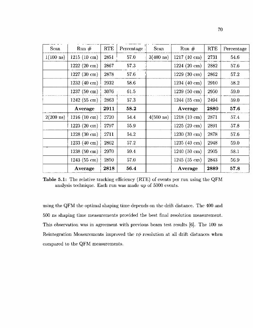
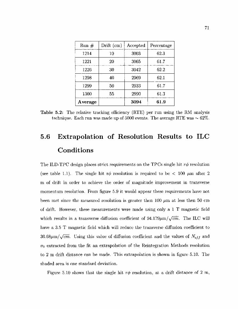
5.8 Average and STD row residual comparison (before and after correction) 73
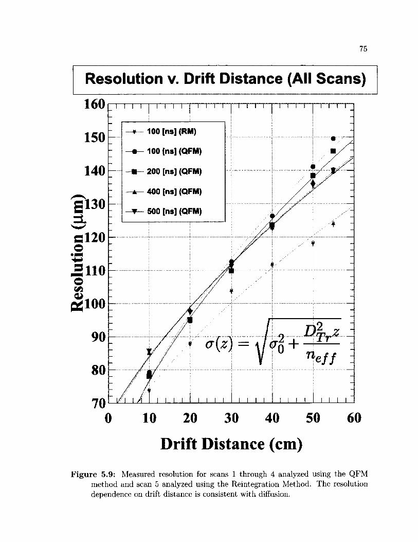
5.9 Single hit r<p resolution vs. drift d is ta n c e ................................................ 75
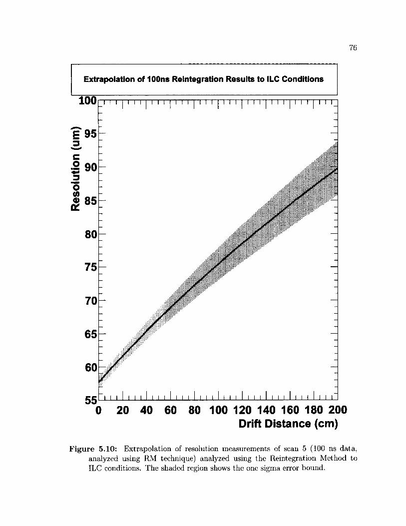
5.10 Extrapolation of Reintegration Method resolution to ILC conditions . 76
List o f Acronym sA FT E R ASIC For TPC Electronic Read out
ASIC Application Specific Integrated Circuit
CEA Atomic and Alternative Energy Commission of France
D E SY Deutsches Elektronen-Synchrotron
FADC Flash Analog to Digital Converter
GEM Gas Electron Multiplier
ILC International Linear Collider
ILD International Large Detector
LHC Large Hadron Collider
LIN AC Linear Accelerator
LP-T PC Large Prototype Time Projection Chamber
M icroM eG as Micro-Mesh Gaseous Structure
M P G D Micro Pattern Gas Detector
PR F Pad Response Function
QFM Quadratic Fit Method
R M Reintegration Method
RTE Relative Tracking Efficiency
RM S Root Mean Square
SiD Silicon Detector
SPM Single Point Maximum
T2K Tokai to Kamioka neutrino experiment, Japan
T PC Time Projection Chamber
1
C hapter 1
Introduction
1.1 T he In ternational Linear C ollider (ILC)
The International Linear Collider (ILC) is a future electron/positron collider intended
to complement the Large Hadron Collider (LHC). The ILC will be able to perform
precision measurements of particles and physical phenomena discovered at the LHC.
The increase in precision of measurements made at the ILC is a result of the nature
of the particles being collided. The LHC, as the name implies, collides hadrons,
which are not fundamental particles. Instead they are a mixture of quarks and gluons
making any interaction between them a complicated multi-body interaction. The ILC,
however, will collide fundamental particles, namely the lightest charged lepton, the
electron, and its antiparticle, the positron. Because these are fundamental particles
they have no internal structure and so any interaction between them is a much simpler
two body collision.
Figure 1.1 shows a diagram of the basic layout of the ILC facility. The initial
phase of the accelerator calls for a total footprint of ~ 31 km. This initial stage will
have a total e+/e~ center of mass collision energy (Ecm) of 500 GeV (250 GeV from
each beam), and a peak luminosity of 2xl034 cm~2s_1, which is a measure of the
number of collisions occurring at the interaction point. A second phase is planned to
2
3
increase the Ecrn to 1 TeV with an additional 11 km of LINACs (linear accelerators)
added to each beam.
Figure 1.1: Diagram of the International Linear Collider layout. In the figure can be seen the electron and positron LINACs, the damping rings (used to compact the particle bunches), the positron/electron sources, and the beam crossing point with the detector system in place. Figure used with permission from the ILD collaboration.
Although the of the ILC is less than that of the LHC, the energy per particle
is comparable. This is again a result of the nature of the particles being accelerated.
The LHC energy is divided amongst the constituent quarks and gluons of each proton.
The ILC’s energy is entirely contained by a single electron or positron.
The ILC is intended to be a facility capable of probing some of the most important
questions still open in particle physics. Central to a broad range of unanswered
questions is the Higgs boson. The Standard Model of Particle Physics requires the
existence of the Higgs boson to give mass to the other elementary particles. Recently
a new boson has been discovered [1] at the LHC which is appears to be consistent
with the Standard Model Higgs. Confirmation that this new boson is indeed the
Higgs boson will require further studies of its physical properties and interactions.
These studies will require the precision available at the ILC.
Model independent studies of the Higgs boson can be conducted at the ILC using
the so-called Golden Channel (see equation 1.1).
e+e“ -> Z°H l+T X , (1.1)
where Z° is a Z boson, l+/l~ are a lepton/anti-lepton pair and X are the decay
products of the Higgs boson. The precision of Higgs studies conducted using the
Golden Channel are limited by the knowledge of the beam energy and measurements
of the final state lepton four momenta. The precision does not depend on the Higgs
decay products, this is what is meant when the Golden Channel is said to be model
independent. Current design requirements for ILC detector system concepts call for
the precision of such a measurement to be ultimately limited by the beam energy. This
means new detector technologies will be required to precisely measure the resulting
leptons.
Currently there are two approved detector system concepts being developed to
meet the requirements for use with the ILC. The first of these is SiD which is a silicon
based detector. The other, the focus of the ILC group at Carleton, is the International
Large Detector (ILD), which will be discussed further in the next section.
1.2 T he International Large D etector for th e ILC
The International Large Detector (ILD) is a detector system intended for use at the
ILC (see figure 1.2). The design philosophy of the ILD, outlined in the 2010 Letter
of Intent [2], is to build a detector which takes full advantage of the well defined
initial state and relative simplicity of interactions provided by a lepton collider. To
this end the ILD intends to couple high granularity calorimeters and a high precision
charged particle tracking system. This will produce a final detector system with
unprecedented spatial and energy resolution of the particle interactions limited
5
Figure 1.2: 3D model of the International Large Detector (ILD) system. The solenoidal magnet is shown in light brown enclosing the entire detector system. The beam pipe can be seen passing through the axis of the magnet. The Time Projection Chamber (TPC) is shown in yellow close to the beam pipe. Figure used with permission from the ILD collaboration [2],
only by the knowledge of the beam energy.
The ILD detector subsystems can be divided into three groups: the beam moni
tors, the detectors dedicated to measuring charged particle momenta and identifying
particle type, and finally detectors intended to identify muons and measure the en
ergy of electromagnetic and neutral particles resulting from interactions. All of these
detectors can be seen in figure 1.2. Upstream of the interaction region in both beam
directions, are the beam monitors. These are responsible for measuring the beam
energy and polarization. Next come the detectors of the charged particle tracking
6
system. These include a Pixel Vertex Detector, then a Silicon Strip Tracker. Sur
rounding these is the main component of the tracker, a Time Projection Chamber
(TPC). Following the TPC are the detectors of the calorimetry group: first the electro
magnetic calorimeter, then the hadronic calorimeter, and finally the muon chambers.
There is also a forward calorimeter which give the system 47r coverage.
The focus of the work conducted by the ILC group at Carleton, and the focus of
this thesis, is the TPC. This detector is called the ILD-TPC and will be discussed in
more detail in the next section.
1.3 T he International Large D etecto r T im e P ro
jec tio n C ham ber (IL D -T P C )
The International Large Detector Time Projection Chamber (ILD-TPC) is intended
to be the central tracker for the ILD. The ILD design calls for a 4.3 m long cylindrical
TPC, divided into two equal sized drift regions by a central cathode, with a diameter
of 3.6 m. This size of TPC will have a readout end plate surface area of 10 m2, which
will need to be instrumented. These detector dimensions are taken from the latest
TPC design report [3]. This large surface area is a driving force for the development of
new readout technologies. The other driving forces are the unprecedented momentum
resolution requirements.
To take full advantage of the possible precision at the ILC, the ILD places strict
design requirements on the momentum resolution for the TPC. The ILD-TPC will
have to significantly improve the single hit transverse (oy^) and longitudinal (<rr2) spa
tial resolution over the traditional TPC design. The spatial resolution requirements
are needed to achieve an order of magnitude improvement in momentum resolution.
7
Apart from the momentum requirements, two track resolutions must also be im
proved. All the resolution requirements for the ILD-TPC are summarized in table
1.1. An explanation of the different spatial resolutions (single hit re/) and rz, as well
as two track r<p and rz) and their effect on momentum resolution can be found in
Appendix C.
Resolution Value Unit
<5 (1 / P t ) 2xl0-5 (GeV/c)-1
& r<f> < 100 f j ,m
(Jr z 0 1 i—1 mm
2 hit r 0 ~ 2 mm
2 hit rz ~ 6 mm
dE/dx ~ 5% -
T able 1.1: Summary of ILD-TPC resolution requirements.
In order to achieve the design requirements of the ILD-TPC novel TPC readout
technologies are being developed. The ILC group at Carleton has focused on the
development of such a readout system. This novel readout utilizes a new class of
amplification structure called Micro Pattern Gas Detectors (MPGDs). MPGDs have
been shown to achieve resolutions on the order of 40 fim with 200 fim wide anode
pads [4]. Use of such narrow pads in the ILD-TPC would require an excessively large
number of readout channels. This complication has been overcome by employing the
process of charge dispersion [5] (described in section 2.4.2) first developed by the ILC
group at Carleton University. Charge dispersion allows for the use of pads which
are an order of magnitude wider, while still achieving the ILD-TPC resolution goals.
The process of charge dispersion is achieved by adhering a resistive foil to the anode
readout pads with a dielectric glue. A TPC which utilizes this improved readout
8
system will henceforth be referred to as a resistive anode MPGD TPC.
1.4 M otivation
The large 1 metre prototype TPC (LP-TPC), used in the present study, was con
structed in 2008 to develop the design for the much larger ILD-TPC. For the present
study the LP-TPC had been equipped with a resistive anode MPGD readout mod
ule. The readout electronics used during the beam test of the resistive anode MPGD
readout module amplify the pad charge pulse from the front-end preamplifier. The
rise time of the front-end preamplifier pulse is larger than its intrinsic rise time due to
longitudinal diffusion of the electron cluster, the induction time of the MPGD, and
charge dispersion. The amplifier shapes the preamplifier pulse with an adjustable
shaping time between 100 and 2000 ns. Existing analysis techniques have shown a
shaping time of 500 ns to achieve the best single hit r r e s o l u t i o n [6]. The 500 ns
shaping time was needed to integrate all electrons contributing to the pad preamplifier
pulse in order to achieve resolution limited only by diffusion and electron statistics.
However, long shaping time pulses require significantly more time to return to
baseline. Figure 1.3 below shows examples of shaped pad pulses digitized by a FADC
(Flash Analog to Digital Converter) for shaping times of 100, 200, 400 and 500 ns. The
slow fall times of pulses from long shaping times will degrade the TPC longitudinal
resolution as well as its ability to resolve multiple tracks.
In order to concurrently achieve both the single point transverse and longitudinal
resolution and prevent signal pile up (resulting in decreased 2 track resolving power),
a new FADC pulse analysis technique using shorter shaping times is required.
9
Main Pad Signal (100ns 30cm drift)
= 2500
<->1500
Main Pad Signal (200ns 30cm drift)
100 110 120 130 140 ISO 160 170Time Bins (40ns)
(a)
Main Pad Signal (400ns 30cm drift)“ 2000
150 160 170Tbm Bins (40ns)
(c)
« 1000
Tims Bins (40ns)
Main Pad Signal (500ns 30cm drift)
£ 2 0 0 0
150 160 170Time Bins (40ns)
(d)
Figure 1.3: Comparison of FADC pulses for different peaking times. Note the time required for FADC pulses to return to baseline increases with shaping time.
1.5 T hesis Layout
This thesis contains the results obtained from the May 2011 beam test of the resistive
anode MPGD equipped LP-TPC. The analysis uses two methods for determining the
single hit r<j> resolution. The first method uses existing pulse analysis technique for
shaping times between 100 ns and 500 ns. The second method, developed for this
thesis, uses a new pulse analysis technique called the Reintegration Method. Because
the shortest possible shaping time is desired, measurements for the Reintegration
10
Method were carried out only for 100 ns data. The results from the different analysis
techniques are then compared.
The thesis proceeds as follows:
1. Chapter 2 covers the fundamental physics of a TPC, as well as the workings of
a traditional wire TPC readout and its limitations. It then goes on to describe
the resistive anode MPGD readout developed by the ILC group at Carleton.
2. Chapter 3 describes the experimental setup used to collect the data analyzed
in this thesis. It describes the TPC readout electronics and how the different
shaping times affect the detector signals. It also describes the different data
sets collected.
3. Chapter 4 explains the steps used in the analysis of the data. The description
starts at the analysis of the shaped FADC pulses and ends with the calculation
of the resolution measurements.
4. Chapter 5 presents the results of the resolution measurements as well as a
comparison of the different techniques. It also contains an extrapolation of the
Reintegration Method resolution measurements to ILC conditions.
5. Chapter 6 summarizes the results obtained and compares them to the ILD-TPC
resolution requirements. Work which must be completed in the future is also
discussed.
1.6 A uthors C ontribution
I contributed to the work presented in this thesis in a number of ways. Firstly, I
actively participate at the DESY beam test of the LP-TPC in May 2011. I ana
lyzed the data collected at the beam test for this thesis. While at the beam test I
11
assisted in the daily operation of the test. This included monitoring detector, beam,
and magnet parameters, changing gas cylinders, and adjusting experimental variables
(drift distances, electronic shaping times, and sampling frequencies). Secondly, while
at Carleton I worked with another student on improving and “cleaning up” of the
analysis code. The improvements to the code included making changes to handle new
data types, implementing new pulse analysis techniques, adjusting data cuts, testing
new functional forms of the pad response function (PRF), and general maintenance
of the code. Thirdly, I was responsible for applying the analysis code to the data
collected. I analyzed 30 separate runs which studied the effects of drift distance and
shaping time on single hit transverse resolution. This part of the analysis was carried
out using existing analysis techniques. My final and most significant contribution to
the work presented in this thesis was the development of a new analysis technique
called the Reintegration Method. The aim of the Reintegration Method was to im
prove the transverse resolution of short shaping time data in order to preserve two
hit resolving power and longitudinal resolution. This new method was applied to the
data first analyzed using the existing analysis techniques. Upon comparison with the
existing analysis methods the Reintegration Method was shown to improve transverse
resolution at all drift distances while employing shorter shaping times.
C hapter 2
Physics o f a TPC
2.1 Fundam entals o f a T P C
A Time Projection Chamber (TPC) is a gas filled particle detector used to study
charged particles. It functions as a high speed 3-D camera that images the ionization
tracks of charged particles which travel through its gas volume. The characteristics
of the track, its radius of curvature (caused by a magnetic field) and amount of
ionization, can be used to measure the particle momentum and to identify the particle
type. Figure 2.1 shows the basic setup and operation of a TPC. As shown in figure
1.2, the ILD-TPC will be cylindrically symmetric with the beam pipe passing through
its axis. In addition to this symmerty the ILD-TPC will also be symmetric about its
central cathode. For this reason figure 2.1 only shows half the TPC when explaining
the basic operation of the detector. The important features shown in the diagram are
the gas volume, the axial magnetic (B ) and electric (E) fields, the central cathode,
and the readout plane which is located on the TPC end plate.
The four steps in the operation of the TPC are shown in figure 2.1. Firstly, (a)
ionization is deposited in the gas volume by the charged particle. The ionization
electrons are then drifted (b) through the gas volume toward the readout plane,
located at the TPC end plate, under the combined influence of the magnetic and
electric fields. Once at the readout plane an amplification structure (c) amplifies
12
TPC Cross Section
13
Beam Pipe
■8O«(TJ0
1 so
ReadoutPlane
Central Cathode(b) (c)
w *'**
■uj.p
Gas Volume Readout Plane
Figure 2.1: Basic setup and operation of a TPC. The smaller diagram shows a cross sectional view of a cylindrical TPC similar to the geometry of the ILD- TPC. The beam pipe can be seen running through the TPC. A central cathode separates the TPC into two drift regions. The operation of the TPC is depicted in the zoomed in view of the upper right section: (a) ionization is deposited in the gas volume by the charged particle, (b) ionization electrons drift and diffuse toward the readout plane (ions drift toward cathode), (c) at the readout plane, an amplification structure amplifies the ionization, (d) the charge created in the amplification causes signal in readout pads. A TPC is symmetric about its central cathode so only half the TPC is depicted in this figure.
14
the ionization. Lastly, the charge created in the amplification causes signals to be
produced in the readout structure (d) on the readout plane.
The first two stages are common to both the traditional wire TPC and the resistive
anode MPGD TPC. The fundamentals of ionization and drifting will be discussed in
the following section. The amplification and readout of the wire and resistive anode
MPGD TPC will then be discussed in following sections.
As a note, the coordinate system shown in figure 2.1 will be used throughout this
thesis. The readout plane is located at 2 = 0 with the origin of the coordinate system
at its center. There are rows of pads extending in the x direction, and columns of
pads in the y direction. The axial magnetic and electric fields are in the positive
z direction. When something is referred to as being transverse or longitudinal it is
with respect to these fields. The gas volume extends from the xy plane into the
positive z region. The resolutions aT(t> and arz also called (transverse and longitudinal
resolutions, respectively) refer to a cylindrical system based on the symmetry of the
TPC. The single hit ar<p resolution refers to the resolution in the v<p plane which is
also the xy plane. Likewise, the single hit arz resolution refers to the resolution in
the rz plane which is in the z direction (into the gas volume).
Although the readout module and readout pads studied in this thesis are keystone
shaped (see section 3.1 for description of the detector) and lend themselves well to
a cylindrical coordinate system, the Cartesian system described above will be used.
There are two reasons for this choice of coordinate system. The first reason is that
the software used to analyze the data studied in this thesis was originally written for
a TPC with a rectangular readout geometry. The second reason is that the readout
pads are nearly rectangular and therefore Cartesian coordinates can still be used to
15
simplify some calculations and descriptions.
2.2 Ion ization and D rift
2.2.1 Ionization
As a charged particle traverses the gas volume of a TPC, it interacts electromag-
netically with the gas molecules producing clusters of ionization. The size of these
clusters (number of electrons) and their frequency along the charged particles path
are probabilistic. The spacing between clusters follows a Poisson Distribution with
a mean which depends on the electron density in the gas and the cross section for
ionization of the gas. The size of a particular cluster is dependent on fluctuations in
the average energy deposited per unit length by the charged particle. Although the
typical cluster has only a few electrons, the cluster size distribution has a long upper
tail caused by rare high energy ionization electrons which cause significant secondary
ionization. The cluster size distribution including this long tail is described by a
Landau curve [7].
The average energy deposited per unit length, d E /d x , is dependent on the particle
momentum and its mass. The dE/dx of a particle is well described by the Bethe-Bloch
equation [8] (equation 2.1).
dE _ 4nNe4 z 2 dx m ec2 f32 In I ^ V ) (2 . 1)
In equation 2.1 N and I are the electron density and mean ionization potential of the
absorbing material. In the case of a TPC the absorbing material is the gas. 8, z, and
7 are the speed (in terms of c), charge, and Lorentz factor of the incident particle.
Lastly, d(/3) is the so-called density effect factor, which accounts for screening of the
incident particle electric field by the atoms of the absorber.
16
Figure 2.2 shows the theoretical dE /dx over a range of momenta for six particle
types calculated using equation 2.1. It also shows the measured d E /d x verses mea
sured momenta for various unknown particles. As the figure shows, this relationship
closely follows the theoretical calculations of dE/dx. Particles can be identified after
their momentum and average energy deposited per unit length have been measured
by referring to figure 2.2.
D t l i . L . . i.~ . iX x l .— .......I....— *—X .X X .i . . . . . .
Cl] 1 10X lnm entum (GeV/r)
Figure 2.2: Scatter plot of average energy deposited per unit distance verses momentum which can be used to identify a particle. Used with permission of the Particle Data Group [9].
As the charged particle traverses the gas volume, its trajectory is bent due to
the magnetic field (shown in figure 2.1). The radius of curvature of the path is
inversely proportional to the strength of the magnetic field and proportional the
particle momentum (equation 2.2),
R = J 4 - 1\B\
(2 .2)
17
Here R is the radius of curvature, \p\ is the magnitude of momentum, q is the charge of
the particle, and |5 | is the magnitude of the magnetic field. If the particle trajectory
is reconstructed, then the radius of curvature can be used to measure the particle
momentum.
2.2.2 Drift
After the ionization electrons have been produced they begin to drift toward the
TPC readout plane under the influence of the electric and magnetic fields. The mo
tion of the electrons as they drift is described by 3 parameters; the drift velocity,
vDrifti arid the coefficients of longitudinal and transverse diffusion DL and DTr, re
spectively. These parameters can be understood by considering a simple model of
electron transport.
A drifting electron in a gas has two components to its velocity, as shown in equation
2.3: a thermal component, Vthermai, and a component resulting from the influence of
the electric and magnetic fields, vfields-
V e le c tro n ~ V th e r m a l T f / i e / d s ( 2 - 3 )
The thermal component of the electron’s velocity has a randomly oriented direction
and a magnitude following a Maxwell distribution. As for the component of the
electron’s velocity caused by the electric and magnetic fields, v fields, since the fields are
aligned vfields is in the same direction as the electric field. The electron is accelerated
by the electric field between collisions with gas molecules.
Immediately after ionization, the electron has only a thermal component to its
velocity. It is then accelerated by the electric field for some amount of time until
it scatters off a gas molecule. Upon this interaction the electron loses the preferred
directionality of its velocity gained from the fields. The time between scattering
18
events follows a Poisson distribution with mean r . This time interval, r , is called the
mean free flight time.
Averaging the stop start motion of the electron over a time t » t (equivalently
over many collisions) the electron’s velocity reaches a steady state. This constant
velocity is called the drift velocity, v D r i f t - When viewed at the macroscopic scale of
the TPC, the electrons drift smoothly toward the readout plane at the constant rate
of VDrijt.
The random motion caused by the thermal component of the velocity results in
diffusion of the electrons in the gas. Initially the electrons are located relatively close
to the point of ionization (disregarding their relatively slow drift toward the readout
plane). However, over time the electron positions become a 3-D Gaussian probability
distribution. The standard deviation of the distribution is described by the coefficient
of diffusion. The diffusion is not isotropic in a TPC. It is suppressed in the transverse
direction by the magnetic field. The dependence of the standard deviations of the
distribution of positions in the transverse and longitudinal directions on drift distance
are shown in equation 2.4.
& T r , L = DTr,L\fz (2-4)
Here z is the drift distance and D T r ,L is the coefficient of transverse or longitudinal
diffusion.
Usually the coefficient of diffusion is given in units of length/ y/time. It is more
convenient in the case of a TPC to define the coefficient of diffusion in units of
length/y/length , where the \Jlength is the drift distance. This is because the amount
of time an electron has been diffusing for is directly related to the distance the electron
has drift. This direct relation is a result of the constant drift velocity, VDrift, of the
electron.
19
Direct calculations of the coefficients of diffusion and drift velocity from the mo
tion of the electrons requires knowledge of the mean free flight time, r , between
collisions with the gas molecules. Values of this parameter are not readily available
or easily calculated. However, the software package Magboltz [10] can calculate these
parameters using a Monte Carlo simulation of electron transport. Values for the drift
parameters, calculated using Magboltz, in the LP-TPC are shown in table 3.1.
It should be noted that the coefficient of transverse diffusion, in table 3.1, is much
smaller then the coefficient of longitudinal diffusion. As mentioned above this is due
to the presence of the magnetic field. Any motion transverse to the magnetic field
has its displacement suppressed because it is forced to travel along a curved rather
than straight line. So after many collisions the total displacement in the transverse
direction is suppressed.
The remaining steps in the operation of the TPC, the amplification and readout,
differ between the traditional wire and the resistive anode MPGD TPC. These will
be discussed in separate sections for each type of TPC.
2.3 T raditional W ire T P C
2.3.1 W ire Amplification
Traditional TPCs have used an anode wire/cathode pad amplification and readout
structure. This setup is illustrated in figure 2.3. Amplification of the electron clusters
occurs around the anode wires which are held at a high voltage. As the electrons
drift closer to the anode they begin to rapidly gain energy in the high field area near
the wire. Eventually the electrons have sufficient energy to begin ionizing the gas
molecules and thus creating secondary electrons. These secondary electrons then go
through the same process of liberating other electrons from the gas. This process is
20
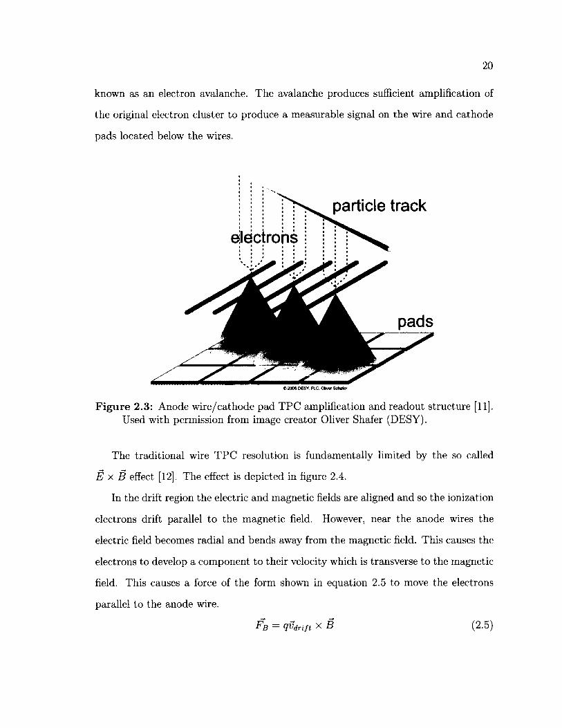
known as an electron avalanche. The avalanche produces sufficient amplification of
the original electron cluster to produce a measurable signal on the wire and cathode
pads located below the wires.
Figure 2.3: Anode wire/cathode pad TPC amplification and readout structure [11].Used with permission from image creator Oliver Shafer (DESY).
The traditional wire TPC resolution is fundamentally limited by the so called
E x B effect [12]. The effect is depicted in figure 2.4.
In the drift region the electric and magnetic fields are aligned and so the ionization
electrons drift parallel to the magnetic field. However, near the anode wires the
electric field becomes radial and bends away from the magnetic field. This causes the
electrons to develop a component to their velocity which is transverse to the magnetic
field. This causes a force of the form shown in equation 2.5 to move the electrons
parallel to the anode wire.
particle track
electrons
e 2006 DESY R.C. Oftvvr Schafer
Fq — ^V'dnjt d B (2.5)
21
Figure 2.4: The E x B Effect. This diagram depicts a view of the readout plane from inside the gas volume of the TPC. The readout pads are shown as blue rectangles, the anode wires can be seen (in gray) stretched out above the rows of readout pads. The clusters of ionization are shown as yellow circles. The different sizes of the circles depicts the differing amount of charge per cluster. The electric field lines near the anode wires are radial to the wire. This causes the electrons to develop a component in their velocity which is transverse to the magnetic field. This results in a rotation of the track segment above each wire. The dashed line separates the segment of the track rotated by the central wire from the segments rotated by the wires above and below.
This results in a rotation of the section of the track above each anode wire. The
E x B effect would be less of an issue if the electron clusters were all about the same
size. However, the cluster size distribution follows a Landau curve so some clusters
are significantly larger than the others. The size of the electron cluster affects the
amount of charge created in the avalanche. In turn, the readout pad amplitude is
proportional to the charge in the electron avalanche. If the clusters were about the
same size the weighted mean would reconstruct the correct avalanche position with
somewhat larger error. However, since the clusters differ in size significantly, the
22
weighted mean cannot accurately reproduce the avalanche position. This is because
a larger cluster will skew the weighted mean toward its location.
The wire TPC is also limited by the large number of positive ions created at the
anode wire during the avalanche process. The ions disrupt the operation of the TPC
in two regions: the amplification region around the anode wires, and the drift region
in the gas volume. The positive ions have a mass which is ~ 2000 times that of the
electrons. Since they are accelerated by the same force the ions travel ~ 2000 times
slower than the electrons. For this reason the positive ions can accumulate around
the anode wires, and only slowly drift away. This reduces the accelerating potential
created by the anode wires reducing the wire gain. Some of the positive ions drift
away from the anode wires and follow the electric field lines back to the cathode at
the opposite end of the drift region. At high rates, these ions can create a significant
space charge which disrupts the electric field in the drift region. Wire TPCs overcome
the limitations imposed by the positive ions by using a gating grid.
These effects (mainly E x B effect) prevent the traditional wire TPC from achiev
ing the resolution goals of the ILD-TPC. They have spurred the development of new
TPC amplification and readout structures.
2.3.2 Traditional W ire T PC Readout
The cathode pads in a traditional wire TPC readout are laid out in rows under the
anode wires (see figure 2.3). The pads generally have an elongated keystone shape
and are aligned with their long axis perpendicular to the anode wires. When an
avalanche occurs a capacitive signal is seen by the pads in the underlying pad row.
The amplitude of the signal seen by the pad is proportional to the distance from the
avalanche. By computing the centroid of pad signals the position of the avalanche
along the wire can be determined.
The path of the charged particle is reconstructed from a number of (x,y,z) points.
23
The number of points is determined by the number of pad rows. The x position
is calculated from the centroid calculation of the pad signals. The y coordinate is
determined from the position of the anode wire which caused the avalanche. The
z coordinate is calculated from the drift time (see equation 2.6). The drift time is
defined as the time between the charged particle entering the gas volume, to (measured
using a fast trigger system), and the time when the avalanche occurs, tsignai (measured
from the timing of the pad pulses). Multiplying this time by the drift velocity,
(which is constant, see section 2.2.2) gives the distance from the readout plane.
Z ~ V d r i f t ( t o ^ s i g n a l ) (2 -6 )
2.4 T he R esistive A node M P G D T P C
2.4.1 Am plification by M ircoM eGaS
The limitations of the traditional TPC readout discussed in section 2.3 prevent such
a TPC from achieving the ILD-TPC resolution requirements. For these reasons a
new type of amplification and readout structure is required. Improvements to the
TPCs resolution can be achieved by employing so-called Micro Pattern Gas Detectors
(MPGDs). Two different types of MPGDs have been developed. The Gas Electron
Multiplier (GEM) [13] and the Micro Mesh Gaseous Structure (MicroMeGaS) [14].
Previous studies have demonstrated the ability of GEMs to achieve the ILD-TPC res
olution requirements using 1 mm wide readout pads [15]. However, complications in
the operation of GEMs with much larger number of readout pads, and their tendency
to damage themselves through sparking at high voltages has lead the ILC group at
Carleton to focus on the use of the MicroMeGaS MPGD.
A schematic diagram of how a MicroMegas functions is shown in figure 2.5. The
diagram is divided into two regions (labelled a, and b, along the right hand side),
and each region is bounded by a plane of constant voltage (labelled HV1, HV2, and
Anode). Region (a) is the drift region. This is the volume of gas where the charged
fTNTI
Anode
READ O UT PLANE
Figure 2.5: Schematic diagram of MicroMegas. (a) represents the drift region and (b) is the amplification region. The MicroMeGas mesh, which separates the drift region from the amplification region, defines a plane of constant voltage labelled HV2. The mesh is supported by insulating pillars not shown in the diagram. The drift field is created by the potential difference between the mesh (HV2) and the central cathode (HV1). the amplification field is created by the potential difference between HV2 and the readout plane (Anode). Due to the proximity of the mesh to the readout plane ( ~ 1 0 0 / i m ) the electric field, even for modest potential differences, is large.
particle would travel depositing clusters of ionization. These clusters then drift to the
amplification region, labelled (b). The drift field is defined by the voltages at HV1
and HV2. These voltages can be set to create a suitable drift field of a few hundred
V/cm. In figure 2.5 the amplification region is divided from the drift region by a
dashed line. This line represents the MicroMeGaS mesh which is a fine metallic mesh
25
with center to center spacing of ~ 25 p.m. The fine spacing of the holes ensures that
the distortion of the electron trajectory is minimized. The spacing between the mesh
and the readout plane, region (b), is ~ 100 pm, this is called the amplification region.
The mesh is supported above the readout plane by insulating spacers called pillars
(not shown). The spacing between pillars is ~ 2 mm ensuring only a few stand above
any one readout pad, preventing distortion of the amplification field. The small gap
between the planes HV2 and Anode produces the amplification field. These voltages
can be adjusted to produce a field of 30 — 40 kV/cm.
The MicroMeGaS amplification structure deals with both factors which limit the
traditional anode wire TPC. Firstly, the resolution of the traditional TPC was limited
by the E x B effect. The MicroMeGaS mesh essentially does not alter the direction of
the electric field thus keeping the electric and magnetic fields well aligned. This min
imizes the amount of transverse motion by the electrons and thus effectively removes
the E x B effect. Secondly, the amount of slow moving positive ions created by the
anode wires of the traditional TPC, could reduce the amplification field of the anode
wires and disrupt the electric field in the drift region. The MicroMeGaS mesh creates
a barrier to the positive ions which efficiently collects the ions and prevents them
from entering the drift region. The high electric field and small distance between
the ions and the mesh quickly removes the ions from the amplification region. This
prevents a build up of positive charge in the amplification region which would reduce
amplification, as was the case in the traditional wire TPC.
2.4.2 Charge Dispersion Readout
The LP-TPC readout module utilizes MicroMeGaS to amplify the electron clusters.
However, due to the proximity of the amplification structure to the readout pads
the resulting electron avalanche is very localized. In previous applications of the
MicroMeGaS this had not been an issue because they had been used to instrument
26
relatively small areas. Instrumenting small areas meant narrow (~ 200 /im) pads
could be used without the large number of readout channels required becoming an
issue. However, the ILD-TPC requires an area of ~ 10 m2 to be instrumented. An
area of this size would require an unmanageable number of readout channels if such
narrow pads were used. To overcome this issue the phenomenon of charge dispersion
is used.
Charge dispersion was first developed and studied by the ILC group at Carleton
University [16]. The process is used to disperse avalanche charge over several anode
pads of the MPGD TPC readout system. The charge dispersion is achieved by forming
a two dimensional resistive-capacitive network on the readout plane.
To produce the 2D RC network a high resistivity (on the order of a few MD/D)
foil is adhered to the readout plane with an insulating glue. Figure 2.6 shows a
cross sectional view of the resistive anode. Any charge which is deposited on to this
foil disperses with an RC time constant much like the charge on a capacitor in an
RC circuit. The RC time constant is defined by the resistivity of the foil, and the
capacitance density between the foil and the readout plane.
Micro Mesh
Avalanche
PCBFigure 2.6: Cross sectional view of the resistive anode which allows for charge
dispersion on the readout plane. The charge from the MicroMeGas avalanche can be seen dispersing across the surface of the resistive foil.
27
The dispersion of the charge on the foil is modelled by the 2D Telegraph equation
shown in equation 2.7.f ) n 1 r r p - n 1
(2.7)dp 1 dt = RC
d2p 1 dp dr2 ^ r dr
In equation 2.7, p(r, t) is the surface charge density at a given location and time, R is
the resistivity of the foil, and C is the capacitance density. The solution for a point
charge deposited at the origin is shown in equation 2.8.
p ( M ) = ^ e x p ( i £ ) ( 2 8 )
Here h — 1 /R C is the inverse of the time constant per unit area of the RC network,
and R and C are the same as in equation 2.7. The raw signal induced on a pad can
be calculated by integrating the time dependent charge density function over the pad
area.
The time/space evolution of a point charge and the induced signal on 3 nearby
pads is shown in figure 2.7. A simulation of the charge dispersion phenomena in a
TPC with MPGD including the effects of diffusion, MPDG rise time, and electronic
timing effects has shown good agreement between the model and measurements [17].
28
third pad3C V U U U { J« U
central pad
p(r,t) integral over pads. . i i . , , . i , .
mm ris
F ig u re 2.7: Surface charge density and the resultant raw charge pulses induced on neighbouring pads [17]. The distribution of surface charge density is shown on the left at five different times between 10 ns and 1000 ns. The figure on the right shows the time dependence of the charge signal seen by 3 different pads. The central pad has observed the charge avalanche directly, whereas the second and thirds pads have seen only the charge dispersion signals.
C hapter 3
Experim ental Setup and D ata Taking
3.1 E xperim ental Setup
The data analyzed in this thesis were collected during a beam test at the DESY
laboratory in Hamburg, Germany in May of 2011. The purpose of the beam test was
to measure the z (drift distance) dependence of the resistive anode MPGD T PC ’s
single hit transverse resolution under different settings of the readout electronics (see
section 3.2). The experimental hall was setup as shown in figure 3.1. The main
components of the setup shown in the figure are,
1. The LP-TPC
2. The superconducting magnet (PCMAG)
3. Moveable stage
4. Electron beam (5 GeV)
5. Readout module
6. Trigger System
This section will describe the important features of each component.
29
30
10m
~6m :
S u p e r c o n d u c t i n g
Magnet
TriggerScinti l lator
<
R e a d o u t
M o d u le
IM o v e a b le
S ta g e
IP TPC
B e a m Entry P oint
ITrigger
Sc inti l la tor
E lectronB e a m
Figure 3.1: Diagram of the experimental setup. The 6 main components of the apparatus can be seen. The motion of the movable stage is shown by the thick arrows.
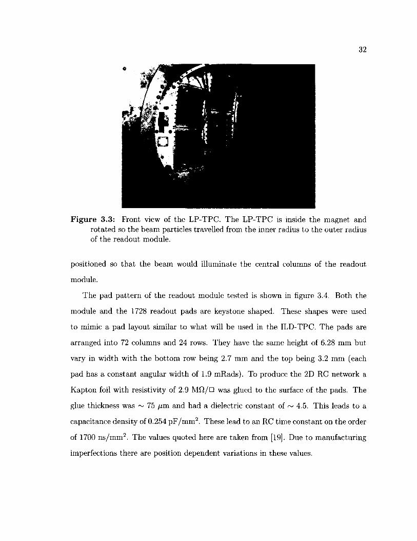
The LP-TPC (side view shown in figure 3.2) is a cylindrical TPC with a diameter
of ~ 80 cm, and a maximum drift length of 60 cm. The end plate contains 7 keystone
shaped ports (see in figure 3.3), arranged in 3 rows, used for testing different readout
modules. Only the central port was used during the present test. The drift volume was
filled with a gas mixture of At /CF^/C^H iq with mixture ratios 95:3:2. The conditions
inside the drift volume were kept at standard temperature and a slight over pressure
to minimize gas contamination. The drift field was set to 230 V/cm and kept constant
throughout the tests. The TPC was placed inside a super conducting magnet.
The magnet, called PCMAG [18], has an inner bore radius of 85 cm and an active
length of 1 m. It is capable of supplying up to a 1.2 T field, though for the purposes of
our tests the field was kept at 1 T. The magnetic field produced has been accurately
Figure 3.2: Side view of the LP-TPC. Note that an older style of readout electronics is attached to the TPC. The new electronics are integrated into the readout module.
measured and even though it contains no iron it has been shown to have a fairly
uniform field in the central region [18]. The LP-TPC was placed close to the center
where the field was most homogeneous. The magnet and TPC were mounted on the
movable stage.
The movable stage allowed the LP-TPC to be kept at the center of the magnet
to ensure a homogenous field but still allowed the location of the beam to be varied
relative to the readout plane. The stage is capable of moving perpendicular to the
beam axis both vertically and horizontally. However, since the resolution as a function
of drift distance was being measured the stage was only used to move the magnet
and LP-TPC horizontally in a direction perpendicular to the beam axis (direction of
motion shown in figure 3.1).
A 5 GeV electron beam with a spread in momentum of A p/p ~ 5%, in the
T22 DESY test beam area [11], was used in the resolution studies. The TPC was
32
Figure 3.3: Front view of the LP-TPC. The LP-TPC is inside the magnet and rotated so the beam particles travelled from the inner radius to the outer radius of the readout module.
positioned so that the beam would illuminate the central columns of the readout
module.
The pad pattern of the readout module tested is shown in figure 3.4. Both the
module and the 1728 readout pads are keystone shaped. These shapes were used
to mimic a pad layout similar to what will be used in the ILD-TPC. The pads are
arranged into 72 columns and 24 rows. They have the same height of 6.28 mm but
vary in width with the bottom row being 2.7 mm and the top being 3.2 mm (each
pad has a constant angular width of 1.9 mRads). To produce the 2D RC network a
Kapton foil with resistivity of 2.9 MD/D was glued to the surface of the pads. The
glue thickness was ~ 75 /Ltm and had a dielectric constant of ~ 4.5. This leads to a
capacitance density of 0.254 pF/m m 2. These lead to an RC time constant on the order
of 1700 ns/m m 2. The values quoted here are taken from [19]. Due to manufacturing
imperfections there are position dependent variations in these values.
33
6 .2 8 m m
1 .9m R ads
F ig u re 3.4: Front view of the readout module. The 1728 readout pads are laid out in a keystone geometry. The pads are arranged into 24 rows each with 72 columns. Due to their keystone shape, pads in the bottom rows are narrower (2.7 mm) than the pads in the top rows (3,2 mm). The pads outlined in orange (those between rows 12 and 23 and columns 30 and 45) were used in the resolution calculation. Initial analysis of the data showed the other pads were not functioning properly.
These variations result in position dependent systematic biases in track position de
termination. These bias errors can be calibrated and are corrected for in the analysis
of the data (see section 4.3.3). The MicroMeGaS amplification structure is attached
above the resistive foil. The MicroMeGaS pillars have a height of 128/im and spacing
of 2 mm. The hole to hole spacing is 63/un. The gain voltage applied to the mesh
was 380 V giving an amplification field of ~ 29.6 kV/cm. The readout electronics are
34
integrated into the readout module and were located outside of the TPC gas volume.
The electronics will be discussed in the next section.
The trigger system shown in the figure 3.1 was used to determine when a beam
electron had traversed the TPC gas volume. Three scintillation counters with at
tached photomultipliers were used to detect the electrons. Two scintillation counters
were located upstream of the TPC and the third was placed downstream. If all three
counters measured a signal, then a signal was sent to the readout electronics to record
data for a sent time window.
Table 3.1 summarizes the experimental parameters which were kept constant
throughout the beam test.
Parameter Name Value Units
Drift Field 230 V/cm
Magnetic Field 1.0 T
MicroMeGas Voltage 380 V
Gas Parameters
Coefficient of Transverse Diffusion D rr 94.2 H m /y/an
Coefficient of Longitudinal Diffusion D i 226.6 lim /y/cm
Drift Velocity vdrift 76.05 [l m /ns
Beam Parameters
Mean Momentum 5.0 GeV/c
A p/p 5 %
Table 3.1: Summary of Experimental Setup Parameters.
3.2 R eadout E lectronics
35
The first studies of a previous resistive anode MPGD TPC undertaken by the ILC
group at Carleton were conducted without shaping the preamplifier pulses [20], [21].
Instead the preamplifier pulses were digitized directly using 200 MHz FADCs (Flash
Analog to Digital Converter). The tests were conducted in this way to study and
understand the new charge dispersion phenomena and to develop techniques to use it
for position determination. Using these 200 MHz FADCs would not have been feasible
at the ILD-TPC due to their cost and the amount of data which would be produced.
Alternatively, a new suite of readout electronics using 25 MHz FADCs could have
been developed. However, due to monetary, manpower and time constraints such a
system was not be developed. In the end the decision was made to adopt the read
out electronics developed for the Tokai to Kamioka (T2K) TPCs [22]. The T2K TPC
electronics utilize the so called AFTER chip [22] readout system developed by CEA
in Saclay, France. The AFTER chip fully integrates the electronics to the readout
module. The new fully integrated electronics contains: front end pre-amp, shaper,
a switched capacitor array to store signals on board, multiplexers/ digitizers, zero
suppression, FADC, and readout drivers. The final digitized data from the module is
readout by a single optical fibre.
The main amplifier shaper of readout systems contains an adjustable shaping time.
The shaper response to an impulse charge has been experimentally measured and
parametrized by the equation 3.1 [23]. Table 3.2 shows parameters for the response
function for different shaping times. Figure 3.5 shows the different response functions.
steps: a raw charge pulse on a pad is amplified in the preamplifier, the preamplifier
(3.1)
Figure 3.6 shows the readout electronics pipeline. The pipeline is made up of four
36
Shaper R esponse Functions |
0.06
0.04
0.02
Time [ns]
Figure 3.5: Examples of the shaper response functions for a range of different shaping times, (black 100 ns, blue 200 ns, red 400 ns, green 1000 ns)
pulse is then sent to the shaper amplifier, the shaped pulse is digitized by a FADC
(at either 25 or 50 MHz), and finally the digitized pulse is stored in memory. The
affect of the pulse shaping on resolution is studied in this thesis.
Shaping Time (ns) Ao b r (ns)
100 0.835065 3 2.05 x 20
200 0.91629 3.5 3.55 x 20
400 0.95396 3.7 7.55 x 20
1000 0.984186 3.85 18.2 x 20
Table 3.2: Summary of response function parameters for different shaping times.
37
Preamp FADC
P a d s A m p lif ie r S t o r a g eFigure 3.6: Signal readout pipeline.
3.3 D ata Taking
The data studied in this thesis were collected in 5 scans. Each scan is made up of 6
runs, which are collections of 5000 events taken at fixed drift distances (10, 20, 30,
40, 50, 55 cm). Each scan studied a different combination of detector settings. The
detector settings which were varied between scans were shaping time (100, 200, 400,
500 ns), and whether to turn on or off the zero suppression process. These detec
tor settings all refer to the readout electronics. The shaping time characterized the
pulse shaping electronics, and zero suppression, a method to automatically record
only nonzero data to limit data set sizes, could be turned on or off. All other de
tector settings were kept constant between scans. These included TPC drift field,
MicroMeGas voltage, and magnetic field strengths, as well as gas composition pres
sure and temperature. Table 3.3 shows an example of scan settings and the runs
which are contained in it. A complete list of scans is given in appendix B.
D ata were collected for all readout pads during the beam test. Initial analysis of
the data showed a number of sections of the readout pad array were not functioning
properly. The readout module being tested was the first of a new design to be built.
This may account for the improper functioning of parts of the readout. Due to
malfunctioning sections, only the pads outlined in orange in figure 3.4 of the readout
array were used in the analysis. The functional pads included those in between rows
38
Scan Parameters Run Parameters
Scan # Shaping Time [ns] Zero Sup. Sampling [MHz] Run # Zrfri/t [cm
1218 10
1225 20
1230 301 500 TRUE 25
1235 40
1240 50
1245 55
Table 3.3: An example of the detector settings used in a scan and the run settings (scan 1).
12 and 23 and between columns 30 and 45 (the pads in other columns may have
worked but we used only the pads in the beam region). Of the pads used in the
analysis not all were used in the calculation of the resolution. The top and bottom
pad rows were not included in the resolution calculation. These rows were omitted
due to the method used to calculate the resolution measurement (see section 4.4).
The data in scan 5 were collected with zero suppression turned off. This was done
because the runs in this scan were analyzed using a new pulse analysis technique.
The zero suppression process affects the recorded pad pulses which would impact
the new analysis technique. It truncates the pad pulses below a certain lower limit.
Charge dispersion pulses generally have slowly rising pulses with low amplitudes in
their leading edge. These time bins, which need to be integrated, would have been
removed by the zero suppression process. The new analysis technique depends on the
full shape of the pulses, including time bins with negative values, and low amplitude
leading edge time bins. For these reasons the zero suppression process had to be
turned off.
C hapter 4
Analysis
4.1 O verview o f A nalysis
The purpose of the analysis is to determine the dependence of the detector’s single hit
T(p resolution on drift distance. The process of determining this dependence has four
steps. Firstly, the signals from the pads must be analyzed and amplitudes determined.
Secondly, these amplitudes are used to determine the trajectory of the charged particle
which traversed the TPC. This is called the track fit. Thirdly, systematic biases in
position determination resulting from imperfections in the detector assembly must be
measured and corrected. And fourthly, after all these steps are taken the resolution
can be measured.
The trajectory of the charged particle which traverses the TPC is reconstructed
from n (x, y, z) points, where n is the number of pad rows. Determination of the
y and z coordinates is the same between the traditional wire and resistive anode
MPGD TPC (see section 2.3.2). The z coordinate is measured from the timing of the
signals and the y coordinate is measured from the position of the pad row. However,
determination of the x coordinate differs.
In the case of a traditional wire TPC the preamplifier pulse has the same shape
for each pad. The only difference is the pulse height which is proportional to the
39
40
distance to the track. The x coordinate can simply be measured by calculating a
weighted mean of the pad amplitudes.
In the case of a resistive anode MPGD TPC the entire pulse shape is dependent
on the track position. This is due to the charge dispersion. The pulse height, rise
time and fall time all differ between pads. Pads which directly observe the charge
have larger pulse heights and faster rise and fall times than pads which only see the
charge dispersion signal. For this reason a simple weighted mean of the pulse heights
will not accurately reconstruct the position of the track (the x coordinate). Instead a
new definition of the pad amplitude is required. Once this new amplitude is defined
its dependence on track position can be characterized by a Pad Response Function
(PRF). This gives us some freedom in defining the amplitude. The definition of the
pad amplitudes used in this thesis are discussed in section 4.3.1.
The PRF relates the distance between a pad center and a track, to the pad
amplitude. Since we are free to define the pad amplitude, the PRF can take many
forms, and all that is needed is a suitable function to parameterize it. In the present
study the PRF has been parameterized by the so-called Product-Form equation,
P R F ( x ) - e x p l - i ‘n ( m - r ) z 2/ w 2}1 + 4r:,:Vw‘ ' >
Equation 4.1 is the product of a Gaussian with a Lorentzian function. The amount
of mixing is defined by the parameter r. When r is 1 the function is fully Lorentzian.
When r is 0 the function is fully Gaussian. Both the Lorentzian and the Gaussian
share the same width parameter w.
Both PRF parameters, r and w, depend on the drift distance of the track, and the
shaping time of the readout electronics. In order to use the PRF to determine the
x coordinate it must first be calibrated to the drift distance of the run and shaping
time of the scan. The method used to calibrate the PRF parameterization will be
41
discussed later in section 4.3.2. Once the PRF has been calibrated it can be used to
fit tracks to the observed pad amplitudes. How the track fitting is accomplished will
be discussed in section 4.2.
Local inhomogeneities in the construction of the resistive anode assembly intro
duce position dependent systematic biases in measurement of the track position.
These biases must be measured and corrected for before the resolution can be cal
culated. Measurements of the inhomogeneities and calculation of the bias correction
are conducted during the analysis. How this is done is discussed in section 4.3.3.
The resolution of the detector is determined from the width of a Gaussian fit to
the global (meaning from all rows) row residual distribution. A row residual is the
difference between the true track position and the fitted track position for the row.
However, because no external reference of the track is available the residuals must be
estimated using equation 4.2 (see reference [24] for a derivation and justification of
this equation).
R = \Z@in&ex (4-2)
Here ain is called the inclusive track fit residual and aex is called the exclusive track
fit residual. The definition of the inclusive and exclusive residuals and how they are
calculated is given in section 4.3.3. An example resolution calculation is shown in
section 4.4.
4.2 Track F ittin g
Figure 4.1 shows an example of a track fit to an event, and the coordinate system
used during the track fitting. The origin of the coordinate system is located in the
middle of the readout plane (between the 12th and 13th row, and the 36th and 37th
columns). Current track fitting procedures fit curved tracks to the data. The track
is described by three parameters, (x0,<p, 1/i?), shown in figure 4.1. In figure 4.1 x0 is
42
the x intercept, (j> is the local azimuthal angle tangent to the track where it crosses
the x-axis, and R is the radius of curvature.
The position, x track, at which the track crosses a given pad row (where the y
coordinate of the pads in the row are y row) is given by equation 4.3,
X t r a c k — X q -f" y r o w t a n {tf>local) (4.3)
In equation 4.3 the angle (f>iocai is the azimuthal angle of the track when it crosses a
pad with midpoint at y r0w-
Y
x ° t -i i\ i 111111 liT m i
IIIHIIIIIHII! !
Figure 4.1: Example of track fitting to an event. Radius of curvature exaggerated to demonstrate track parameters.
43
A chi-square minimization is used to determine the track parameters. The chi-
square minimized to fit the track is given in equation 4.4,
X track ^ ̂Xrow = £ £Aj A 1peakP R F (xlj X t r a c k )
aA\(4.4)
Here the first sum is over all the pad rows used and the second is over the pads in each
row which recorded an amplitude above a threshold value (in figure 4.1 those would
be the coloured pads). The variables A* and x* are the amplitude and position of the
j th pad in the ith row. The scaling factor, Apeafc, is calculated for each row individually
by minimizing Xrow w^ h respect to A % k. The value of Alpmk which minimizes Xrow
is found by taking the derivative of xfow wbh respect to A lpeak and setting the result
equal to zero. Then solving for A lpeak finds the value of Apeak which minimizes Xrow-
The result of this process is given in equation 4.5,
A ) P R F ( x *)
a* ________ j (a eopeak PRFHA) ’ V }
^>3 AA 1.3
where .x* and A* are the same as in equation 4.4. The error, aA,., in equations 4.4
and 4.5 was set to the square root of the pad amplitude.
The initial guess of the track used in the chi-square minimization is called the
seed track. The pads in each row with the largest amplitudes, called the primary
pads, are used to determine the seed track. A linear least squares fit is applied to the
positions of the primary pads and the resulting fit parameters define the seed track.
The inverse radius of curvature of the seed track is always set to 0.
4.3 A nalysis P ip e lin e
44
This section will describe the analysis pipeline starting from the raw pad signals and
ending with the calculation of the detector single hit r</> resolution. The analysis is
made up of four separate steps. These steps can be seen schematically in figure 4.2.
FADC Pulse Analysis
IPRF
Calibration
I
Bias Correction
IResolution Calculation
F igu re 4.2: Schematic of the analysis pipeline.
The analysis pipeline is applied to each run individually. The first of these steps
computes a pad amplitude and time measurement from the shaped pulses of each pad.
The time measurement is not used in the calculation of the transverse resolution but
will be included in this description for completeness. These values are then stored in
what are called dense data (DD) files. The next step uses the values in the DD files to
calibrate the PRF for the given run. Once the PRF has been properly calibrated the
next step is to calculate a bias correction for each pad row in the detector. Finally, the
DD file, PRF, and bias corrections are used to calculate the resolution of the detector.
These four steps in the the analysis pipeline will be described in more detail in the
following subsections.
45
4.3.1 Calculation o f Pad A m plitudes
The amplitude and time are calculated using some defining feature of the shaped pad
pulses. There are three methods which have been used to determine the amplitude
and time measurement. This section will give a description of each method.
The pulse analysis method which had been used in previous studies is known as
the Single Point Maximum (SPM). This defines the amplitude as the largest FADC
value in the pulse and uses the value of the time bin of the largest pulse as the
time measurement. While this can produce a useful value for amplitude, the time
measurement is quantized to the widths of the FADC bins (either 40 ns or 20 ns
depending on the sampling frequency used). As well, both the time and amplitude
measurements are significantly affected by noise. This effect is more pronounced in
pads with lower pulse heights as the amount of noise is independent of pulse height.
An example of this SPM method is shown in figure 4.3.a.
An improvement to the SPM method is the Quadratic Fit Method (QFM). This
method finds the largest FADC value and the four time bins surrounding it. These five
points are then used to fit a quadratic function (see figure 4.3.b). The maximum point
of the fitted quadratic is then used to define the time and amplitude measurements.
This method improves both the amplitude and the time measurements compared to
the SPM. The time value is no longer quantized to the time bin widths of the FADC.
As well, both the time and amplitudes are less affected by noise since the fit averages
the values over more than one time bin. This method of pulse analysis will be used
to produce baseline measurements of the x<p resolution. These baseline measurements
will then be compared to the results obtained using the new pulse analysis technique
described next.
The new method, which is the focus of this work, is used presently only for de
termining the amplitude and would require another method for determining the time
46
Main Pad
120 140 160 100 200 220 240
Time Bins (40ns)
1st Neighbour
100 120 140 100 110 200 220 240
Tims Bins (40ns)
.1 i 2nd Neighbour
'lOO 120 140 100 100 200 220 240Time Bins (40ns)
(a)
12001000
800000
4002000
Main Pad
100 120 140 160 180 200 220 240
Time Bins (40ns)
oOoQ<Ul
1«t Neighbour
140 160 180 200 220 240
Time Bins (40ns)
100 120 140 160 180
2nd Neighbour
^16^^18^^20^^22^^240Time Bins (40ns)
(b)
Figure 4.3: Examples of the pulse height analysis techniques, a) Single Point Maximum (SPM), b) Quadratic Fit Method (QFM).
measurement. The amplitude is calculated by integrating the FADC pulse over a fixed
window. The integration is defined by two numbers: the starting time bin, T star t, and
the integration width, to. Presently the same width is used for an entire scan and is
calibrated to give the best resolution. The starting time bin changes between rows
depending on the FADC pulse of the pad in each row with the largest signal and is
found using the following method. The RMS of the noise, crrms, is calculated from the
first 20 bins of the FADC pulse. The RMS of the noise is found by first calculating
the average FADC value, A , in the first 20 bins. Next A is used to find a rm s using
equation 4.6. ______________
(4.6)N - 1
where Aj the FADC value in the ith time bin, and N is the number of time bins used
47
(20 in this case). To avoid signal being located in the bins used to calculate the RMS
of the noise extra time bins were record before the actual signal arrived (see figure
4.4). The first time bin, Tsignat, with a signal greater then 4arms is then located.
This time bin is located in the actual pulse. To ensure the beginning of the pulse is
included in the window, Tstart is located 3 time bins before Tsignai, (see figure 4.5).
The pad amplitude is then calculated using equation 4.7,
t s t a r t ~
A = £ A . (4.7)i = t s t a r t
where A{ is the value in the ith FADC time bin and A is the resulting integrated pad
amplitude.
The rationale for the Reintegration Method is as follows. Short shaping times are
not long enough to fully integrate the preamplifier pulse. As a result the peak height
of a short shaping time pulse is not an accurate measure of the charge seen by the
pad. The information contained in the entire shape of the pulse, however, can be
used to get a better estimate of the total charge seen by the pad. The Reintegration
Method uses the information contained in the shape of the pad pulse to calculate
the pad amplitude. The pad amplitude calculated using the Reintegration Method is
then a better estimate of the total charge seen by the pad.
4.3.2 PR F Calibration
The PRF could be measured directly if an external measure of the track position
was available. A similar measurement was conducted using a fixed collimated x-ray
source [16]. Since no precise external measurement of the track is available for the
LP-TPC, the PRF must be calibrated using another method. The technique uses an
iterative approach which requires an initial guess of the PRF parameters. It relies on
internal consistency of the data to ensure an appropriate PRF is found.
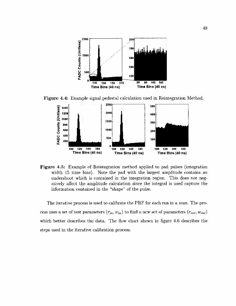
Time Bins (40 ns) Time Bins (40 ns)
Figure 4.4: Example signal pedestal calculation used in Reintegration Method.
100 120 140 160Time Bins (40 ns)
100 120 140 160Time B ins (40 ns)
100 120 140 160Time B ins (40 ns)
Figure 4.5: Example of Reintegration method applied to pad pulses (integration width 15 time bins). Note the pad with the largest amplitude contains an undershoot which is contained in the integration region. This does not negatively affect the amplitude calculation since the integral is used capture the information contained in the “shape” of the pulse.
The iterative process is used to calibrate the PRF for each run in a scan. The pro
cess uses a set of test parameters (rin, wlTl) to find a new set of parameters (rout, wout)
which better describes the data. The flow chart shown in figure 4.6 describes the
steps used in the iterative calibration process.
st I
F ig u re 4.6: This flow chart shows the steps used in the iterative PRF calibration process.
50
To start the iterative process, initial guesses of the PRF parameters are required.
For most runs initial guesses of r = 0.5 and w = 3.5 were used. This started the PRF
as half Gaussian, half Lorentzian, and with a width about the same as a single pad.
The initial set of PRF parameters was then used to perform all the track fitting in
the run. Only events which passed the event selection rules described in appendix A
were used. After tracks have been fit to all the successful events, the values shown
in equations 4.8 and 4.9 were recorded for each pad with an amplitude greater than
some threshold value, determined by noise.
Ax = X lp a d - X tr a c k (4.8)
Anorm = Ai/Apeak (4-9)
In equation 4.8 Ax is the distance between the ith pad (located at xpad) and the
track (located at x track). In equation 4.9 A norm is the normalized amplitude of the i th
pad, Aj is the amplitude of the i th pad, and Apmk is the peak amplitude described in
section 4.2.
The values Ax and Anorm are then used to create a scatter plot of Ax versus
A norm- An example of such a scatter plot is shown in figure 4.7. This scatter plot is
the combined measurement of the PRF from all events in the run.
The scatter plot is then divided into 86 bins of equal width and the average of each
bin is calculated. These 86 points are then used to fit the functional form (equation
4.1) of the PRF, figure 4.8. From the fit two new parameters ( r ^ , u w ) and the chi-
square value Xnew °f the fit are retrieved. To determine whether the new parameters
better describe the data Xnew is compared to the total chi-square value of the previous
iteration, xlid-If Xnew smaller than xlut? then the PRF defined by (rout, wout) better describes
the data and these parameters are used as the initial guess of the next iteration.
51
oc
0.8
0.6
0.4
0.2
AX (mm)
F ig u re 4.7: Example scatter plot of AX vs. A norm. From the the PRF calibration of run 1230.
Otherwise, Xnew greater than xhd, the iterative process is ended and the parameters
(rin, win) are the properly calibrated PRF parameters. In the case of the first iteration
where no xhd value is available the comparison is skipped and a second iteration is
automatically conducted.
To test whether the iterative approach produces a valid PRF, the behaviour of
the PRF parameters as a function of drift distance is checked. This check is done
after the PRF has been determined for a full scan of the TPC. One would expect the
parameters to display a smoothly varying dependence on drift distance. In particular,
the PRF is expected to become wider with increasing drift distance. This widening
is due to diffusion, and charge dispersion.
For the present functional form of the PRF the r parameter is expected to decrease
and the w parameter is expected to increase as a function of drift distance. Both of
these behaviours are caused by the increase in diffusion resulting from an increase
in drift distance. An electron cluster which drifts further will become wider due to
52
1.265c
<
0.8
0.6
0.4
0.2
A X (mm)
Figure 4.8: Example fit of equation 4.1 to the binned scatter plot of A x vs. Anorm. From the PRF calibration of run 1230.
diffusion. As the cluster becomes more diffuse the amount of charge dispersing from
any one point decreases and the charge dispersion signals becomes less prominent.
This will result in a wider and more Gaussian PRF. Diffusion causes the electron
cluster to take on a Gaussian profile and this results in an increase in the weight of
the Gaussian in the PRF. To account for this, the r parameter becomes smaller which
increases the weight on the Gaussian portion of the PRF. The increase of w is natural
because it is the width parameter of both the Gaussian and Lorentzian.
4.3.3 Bias Corrections
Due to imperfections in the construction of the resistive anode assembly leading to
local variations in the RC parameters, each row has a position dependent systematic
error associated with its track position determination. A bias correction is calculated
to account for this systematic error before the final resolution of the detector is mea
sured. Bias corrections are calculated separately for each row. They are calculated as
a function of position along a row and are made up of averaged row residuals. This
53
section will explain how equation 4.2 is used to calculate row residuals. It will then
explain how the bias correction is found from the row residuals and how it is applied.
Before a more rigorous description of row residuals is given, and how they are
used to calculate bias corrections and resolution, a more qualitative description will
be discussed.
Since no external measure of a track is available, a comparison between the true
track and measured track is not possible. This would be the typical way of accessing
the resolution of the detector. However, by relying on the internal consistency of the
track positions measured by each pad row in the TPC, a similar comparison can be
made.
To determine the resolution of the detector overall first the resolution of each pad
row is measured. These row resolutions can then be combined later to determine the
resolution of the detector. To measure the resolution of a single row, called the test
row, a more accurate determination of the track must be made then can be achieved
by the test row alone. This more accurate measurement, the inclusive or exclusive
track fit mentioned previously, is achieved by using all the pad rows (inclusive track
fit) or all the pad rows except the test row (exclusive track fit) in the detector to fit
a track. The test row is then used individually to determine the position of the track
above the test row. This measurement of the track position by the test row is called
the single row track fit. The position predicted by the inclusive or exclusive track
fit can then be compared to the position predicted by the single row track fit. The
difference between the predicted track positions is called the row residual (of the test
row). In the case where the inclusive track fit is used it is called the inclusive row
residual, and in the case where the exclusive track fit is used it is called the exclusive
row residual.
The reason for the two types of track fits (inclusive and exclusive) is that the
residual calculated by each individually are incorrect. The inclusive row residual is
54
too small and the exclusive row residual is too large. However when combined using
equation 4.2 they produce a more accurate estimate of the true row residual.
By collecting the row residuals calculated from equation 4.2 a measurement of the
error in the determination of track position by a row can be made. How this can then
be used to correct for position dependent bias in a row is discussed in section 4.3.3.
How the row residuals are used to calculate the detector resolution is then described
in section 4.4.
Row Residuals
As mentioned in the analysis overview (section 4.1) the row residual is estimated using
equation 4.2. This equation estimates the row residual of a test row using the so-called
inclusive, ain, and exclusive, aex, track fit row residuals. An inclusive row residual
is calculated from a track fit which includes the test row. An exclusive row residual
is calculated from a track fit which does not include the test row. As mentioned
previously both inclusive and exclusive residuals are required because individually
their estimates are incorrect.
The inclusive and exclusive row residuals are calculated using equation 4.10 and
4.11, respectively.
& in X tr a c k X tr a c k ' (4-10)
ex A r a c k ~ A r a c k ' t 4 ' 1 1 )
where x™ack and x ^ ack are the track positions on the test row for the inclusive and
exclusive track fits respectively. The position x'track is the single row track fit. The
single row track fit is calculated by minimizing the chi-square in equation 4.12 with
55
respect to x'track.
Aj — A peakP RF(xi — x track)x2 = YA.rcrw / j (4.12)
Where x'track is the position of the track on the test row as determined by the test
row itself.
C alculation o f Bias Correction
The bias correction is calculated after all the row residuals have been found. The
residual for each row and the inclusive track fit parameters are recorded. Using the
inclusive track parameters the track position on each row, x)"ac(t, is calculated. This
value is then plotted against the row residual for that track in separate plots for each
row. After all the tracks have been analyzed a scatter plot is produced for each row.
Figure 4.9 shows an example of such a scatter plot for the 13th pad row of the readout
plane.
The scatter plot is then binned into forty bins and the average residual in each
bin is calculated. These forty points sample the bias correction function at equally
spaced steps (step size is 0.5 mm). Figure 4.10 below shows an example of the
resulting histogram after binning and averaging the scatter plot shown in figure 4.9.
A spline interpolation is used to evaluate the bias correction function between points.
The bias correction is used during the track fitting and row residual calculation
processes. The correction is applied whenever the PRF must be evaluated on a row.
For example, when performing the single row track fit or the inclusive/exclusive fit
the minimized Xrow becomes,
x 2Araw / jAi ApeakP R F ( X i ■X'track "f" B i a s ( x t r a c k ) }
<JAl(4.13)
56
I Row13 |0.5IM0.3
"flj 0.2
-Q 0.1
'35<D
-o.i - 0.2
-0.3
-0.4
■ - . . ’ -
■; !'•* .
’ ]■
: • a- ■ v - T r M v . . V' £ ' K V v , \
— . • V •
-1 , 1 , ,
t : : '■ ■: T ^ ::C i't'Z1/' &‘-s •: - ?^?7 * : ‘
r ■ ■
" * * * !'j‘7 ■ ■' • . i '
L. . .1 . :i----1 - i - I i i i i
■r ~ , .• v.f J
. . , . 1— -10 -5 0 5 10
X (mm)row' ' <|Bias|>: 46.1 um , STD: 65.9 urn
F ig u re 4.9: Example of a scatter plot of row residual verses x™ack for the 13th row of the detector.
where Bias{xtrack) is the bias correction function evaluated at the point where the
track fit crosses the row.
After applying the bias correction to the track fitting the resolution can be calcu
lated. Figures 4.11 and 4.12 show the row residual of row 13 after the application of
the corrections. Note the reduction in row residuals across all pads in the row.
Two other consistency checks are conducted after the application of the bias cor
rections. After the row residuals for each row are plotted as in figures 4.10 and 4.12
two values are calculated. The average absolute value of the residuals and the stan
dard deviation of the absolute value of the residuals are calculated (they can be seen
under the x-axis of figures 4.10 and 4.12). These values are then compared for the
row residual distributions before and after the application of the bias correction. If
the average and standard deviation both decrease then the bias correction has been
F ig u re 4.11: Example of a scatter plot for the 13th row of the detector after the application of the bias corrections.
for the middle pad rows. When performing the exclusive track fit on a test row in
the middle of the readout module, the rows above and below the test row constrained
the fitted track. However, when the exclusive track fit is performed on the top and
bottom rows the fitted track is not constrained. The resulting track does not take
into account the trend of the top or bottom row.
4.5 D ep en d en ce o f R eso lu tion on D rift D istan ce
After all the runs in a scan have been analyzed the relationship between single hit
r<p resolution and drift distance can be plotted (see figure 5.9). If the resolution
dependence on drift distance is consistent with the effects of diffusion and electron
statistics, as has been observed in previous studies [20] [25] [24], then the measured
59
I Row13 |
(0 0.2 E-
3 « i -
-0 .2 E -
-0.3
-0.4
-0.5 -10 -5 0 5 10
X (mm)row'<|Bias|>: 23.8 wm , STD: 31.3 um
F ig u re 4.12: Example of a binned and average row residual scatter plot for the 13th row of the detector after the application of the bias corrections.
resolution as a function of drift distance should follow equation 4.14.
Equation 4.14 shows the single point transverse resolution has 2 components. The
first component, a0, is the intrinsic component of resolution resulting from noise in
the detector. The other component is the result of diffusion which depends on the
When combined as in equation 4.14 these two terms are the variance of the estimated
mean position of an electron cluster from a sample size of ne//.
Equation 4.14 function is fitted to the measurements of transverse resolution.
Before equation 4.14 can be used to fit the experimentally measured resolution, a
value for Dtr must be found. As mentioned previously (section 2.2.2) this value can
(4.14)
width of the electron cluster D\Tz and the effective number of electrons observed nej f .
F ig u re 4.13: Examples of the global residual distributions and corresponding normal distribution fits for for runs 1226 (100 ns), 1228 (200 ns), 1229 (400 ns), and 1230 (500 ns).
Resolution Fit For Run #1230 Resolution Fit27783Entries
be calculated using the Monte Carlo program Magboltz.
The resulting fit parameters (<j0 and A e//), from the fit to scan 5 measurements,
were also used to extrapolate the r<p resolution found using the Reintegration Method
to 2 m of drift. To complete the extrapolation the coefficient of transverse diffusion
must be recalculated. This recalculation is required to due the dependence of D7>
on magnetic field strength. The measurements of the V(j> resolution made with the
LP-TPC were conducted with a 1 T magnetic field, whereas the ILD-TPC will be in
a 3.5 T magnetic field.
C hapter 5
R esults
The outcome of the intermediate analysis steps will be presented in the same order
as the analysis was conducted. Firstly, the optimization of the integration width,
needed for the Reintegration Method, will be presented. Secondly, the calibrated
PRF parameters for all 5 scans will be shown along with the outcome of the PRF
parameter validation test. Next the calculation and application of the bias corrections
and the outcome of the bias consistency checks will be presented. Following this the
results of the single hit r</> resolution measurements for all 5 scans will be presented
and compared. Finally, the extrapolation of the Reintegration Method resolution
measurements to the ILD-TPC conditions will be presented.
5.1 O ptim ization o f In tegration W id th
In order to use the Reintegration Method to calculate pad amplitudes, an integration
width, uj, must be chosen. This width will be the range over which the pad pulse will
be integrated (as discussed in section 4.3.1). In order for the Reintegration Method
to produce the best possible results, ui must be optimized. To determine the optimal
integration width, u> was varied between 10 and 35 time bins and the resolution
measured. Since the technique was applied to data collected at a FADC sampling
62
63
rate of 25 MHz, this corresponds to integration widths between 400 ns and 1400 ns.
These optimization measurements were conducted using run 1226 (30 cm drift, 100
ns shaping time, none zero suppressed). The results of these calculations can be seen
in Figure 5.1.
Optimization of Integration Width120
S118
2 116
114
112
110
108
106
5 10 15 20 25 30 35 40Time Bins [40ns]
F ig u re 5.1: Determination of optimal integration width. Note errors on resolution are set equal to the error on the Gaussian width fit to the residual distribution.
From figure 5.1 it is seen that the optimal integration width is 15 bins. This value
was applied to all the amplitude calculation in the runs of scan 5.
5.2 P R F C alibration
Figures 5.2 and 5.3 show the calibrated PRF parameters for scans 1 through 4 (scan
parameters listed in appendix B) as a function of drift distance. These scans were
analyzed using the QFM pulse analysis technique. Figures 5.4 and 5.5 show the same
plots for the PRF parameters obtained for scan 5, which was analyzed using the
Reintegration Method. In both cases the calibrated PRF parameters satisfy the first
64
validation check of the analysis, a smoothly varying dependence on drift distance (see
section 4.3.2). The shape of the PRF is governed by diffusion which increases as a
function of drift distance. For this reason the PRF parameters should also show a
monotonic behaviour as a function of drift distance. The PRF parameters for both
analysis techniques showed a monotonic behaviour with increased drift distance.
PRF Param eter ’r' vs. Drift Distance
2 0.9
0.8lOOnt
0.78
0.76
0 10 20 30 40 50 60Drift Distance [cm]
F ig u re 5.2: Calibration results for scans 1 through 4 of the PRF mixing parameter r. These scans were analyzed using the QFM method. An r value of 1 produces a fully Lorentzian PRF and 0 a fully Gaussian PRF. The trend shows the PRF becoming more Gaussian-like as drift distance increases. Note errors (statistical component only) on PRF parameters to small to be seen on graph.
Figures 5.2 and 5.4 show that the mixing parameter r decreases with increased
drift distance for both the QFM and Reintegration Method. This is consistent with
diffusion, as discussed in section 4.3.2. The PRF of the Reintegration Method dis
plays a more Gaussian shape than the QFM PRF, irrespective of shaping time. The
Reintegration Method also shows a quicker decrease in the mixing parameter of its
PRF than the QFM PRF. This is demonstrated by the quadratic dependence on drift
distance seen in the mixing parameter of the Reintegration Method PRF as opposed
to the linear dependence of the QFM PRF mixing parameter.
65
**£sseE>to£
fta.
PRF Parameter V vs. Drift Distance
-..........¥...*’*
“ ...A- •" ....
- ___
.............
L. . . . 1 . . . . 1 . . . . 1 . . . . 1 .
100ns-•-2 0 0 n s
400ns500ns
Drift Distance [cm]
F ig u re 5.3: Calibration results for scans 1 through 4 of the PRF width parameter ’w’. These scans were analyzed using the QFM method. The width increases as a function of drift distance as can be expected due to diffusion. Note errors (statistical component only) on PRF parameters to small to be seen on graph.
Figures 5.3 and 5.5 show an increase in width parameter, w, with increased drift
distance for both analysis techniques. These trends are again consistent with predic
tions resulting from diffusion. Both techniques produce PRFs with width parameters
displaying a linear dependence on drift distance. However, the width parameter of
the Reintegration Method PRF is significantly wider then the QFM PRF at all drift
distances. The rate of increase in w is comparable between techniques, and across all
shaping times.
Figures 5.6 and 5.7 show the PRFs determined for both analysis techniques and
all shaping times. Figure 5.6 compares the PRFs at 10 cm of drift (shortest measure
ment). Figure 5.7 shows the same comparison at a drift distance of 55 cm (longest
measurement). As can be seen in these figures the Reintegration Method produces a
more dynamic PRF than the QFM. The vertical dashed lines represent the location
and width of the average pad in the readout plane. The pad amplitude predicted by
the PRF is the value of the PRF at the pad’s midpoint. In figures 5.6 and 5.7 the
66
PRF Parameter V vs. Drift Distance
100ns Reintegration.
L_ ... L _1. 1 !■ _t._ ..I. L 1 _L . I- . .i_ _ _l_. . 1 .. 1- 1 ■ 1 » I- I - -I. »- t 1*1 I
"0 10 20 30 40 50 60Drift Distance [cm]
Figure 5.4: PRF parameter ’r ’ as a function of drift distance for scan 5 analyzed using the Reintegration Method. An ’r ’ value of 1 produces a fully Lorentzian function and 0 a fully Gaussian. The trend shows the PRF becoming more Gaussian like as drift distance increases. Note errors (statistical component only) on PRF parameters to small to be seen on graph.
neighbouring pad midpoints are at ±3 mm.
At short drift distances the RM PRF predicts an amplitude on the neighbouring
pads of ~ 12% that of the main pad. This value is in between the short shaping
time (100 and 200 ns) and long shaping time (400 and 500 ns) QFM PRF predic
tions. At long drift distances the RM PRF matches the 500 ns QFM PRF with a
neighbouring pad amplitude of ~ 20% that of the main pad amplitude. At all drift
distances the Reintegration Method PRF decreases to zero within ~ 5 mm. This is
similar behaviour to the 100 ns and 200 ns QFM PRFs. This adaptability of the RM
PRF may contribute to the Reintegration Method’s improved transverse resolution
measurements.
The PRF parameters determined in this section were used to complete the rest of
the steps in the analysis pipeline. The parameters will also be useful to analyze data
taken in the 7 modules test conducted in July of 2012.
«f0.552.> 0.5 1
£ 0 A&“-0.35
0.3
0.25
67
1 3.9Sie2.> 3.8
j„a. 3.6 a.
3.5
3.4
PRF Parameter 'w' vs. Drift Distance
—-
—- ■» +
y '*
y* y
**
¥
+ 100ns Reintegration.
” 1 1 1 . / 1 t .. 1 .1. 1 ... i ...X .1 ..X .X .. _i_ I i » ■ i—l-_t- i— i —>0 10 20 30 40 50 60
Drift Distance [cm]
Figure 5.5: PRF parameter ’w’ (width) as a function of drift distance for scan 5 analyzed using the Reintegration Method. The width increases as a function of drift distance as can be expected due to diffusion. Note errors (statistical component only) on PRF parameters to small to be seen on graph.
5.3 R ela tive Tracking Efficiency
The relative tracking efficiency (RTE) of a run is defined as the ratio of events which
pass the event selection cuts (details of cuts given in appendix A) to the total number
of events taken in that run. Table 5.1 and table 5.2 summarize the RTE for each
run after the application of event cuts for the QFM and Reintegration Methods,
respectively. An average RTE of ~ 62% was observed for the Reintegration Method.
The RTE for the QFM method varied depending on shaping time. The average RTE
for the QFM was ~ 58%.
The measured resolution of a run can be artificially improved by decreasing the
number of events which pass the event selection cuts. By allowing only those events
which have a high signal to noise ratio to be analyzed the measured resolution would
not be representative of the detectors abilities to measure the average track. Since
the RTE for the Reintegration Method was similar to that of the QFM RTE, we can
68
•g 0.8| a E< 0.6 u. tc cl
0.4
0.2
°-5 -4 -3 -2 -1 0 1 2 3 4 5x [mm]
Figure 5.6: Comparison of the PRFs, at short drift distance, determined for both analysis techniques and all shaping times. The vertical dashed lines represent the average pad width.
be confident that the resolutions measured using the Reintegration Method were not
artificially improved through too restrictive event selection.
5.4 B ias C orrection
The bias corrections were calculated as described in section 4.3.3. The second and
third consistency checks (also described in section 4.3.3) of the data were performed
after applying the corrections to the track fitting procedure. In order to quantitatively
express whether the bias correction had indeed decreased the position dependent
biases in track position determination, the weighted average of the absolute value of
row residuals and weighted standard deviation of the row residuals were calculated
from the separate row residual scatter plots.
The weighted means and standard deviations (see figure5.8), for the row residuals
both before and after application of the bias correction, were collected and displayed
PRF Comparison (z=10cm)
100ns(RM) 100n*(QFM) 200ns 400ns 500ns
69
PRF Comparison (z=55cm)
100ns(RM)lOOns(QFM)200ns400ns500ns
■“P ^ r T i l i i i i I i i i i I i i i i I i i i .i ..I i i i_i I i i i_i Li i i i_l i—i i i X T frrr& s•5 -4 -3 -2 -1 0 1 2 3 4 5
x [mm]
F ig u re 5.7: Comparison of the PRFs, at long drift distance, determined for both analysis techniques and all shaping times. The vertical dashed lines represent the average pad width.
in the bar graphs of weighted mean (top) and standard deviation (bottom) versus row
number. As the graphs show, there was a significant reduction in position dependent
biases in all rows.
5.5 R eso lu tion M easurem ents
After the calculation and application of the bias corrections, the resolution for each
run was measured. The method for determining the resolution is described in section
4.4. The measured resolution values with uncertainty are summarized in table 5.3.
The error values included in the table were taken from the uncertainty on the fit to
the global residual distribution for that run as described in section 4.4.
Each scan was used to plot a graph of measured resolution versus drift distance,
and equation 4.14 fitted to the measurements. These graphs were collected and
plotted together in figure 5.9. Among the measurements of rr/> resolution obtained
70
Scan Run # RTE Percentage Scan Run # RTE Percentage
Table 5.1: The relative tracking efficiency (RTE) of events per run using the QFM analysis technique. Each run was made up of 5000 events.
using the QFM the optimal shaping time depends on the drift distance. The 400 and
500 ns shaping time measurements provided the best final resolution measurement.
This observation was in agreement with previous beam test results [6]. The 100 ns
Reintegration Measurements improved the r4> resolution at all drift distances when
compared to the QFM measurements.
71
Run # Drift (cm) Accepted Percentage
1214 10 3003 62.3
1221 20 3065 61.7
1226 30 3042 62.2
1298 40 2969 62.1
1299 50 2933 61.7
1300 55 2990 61.3
Average 3094 61.9
Table 5.2: The relative tracking efficiency (RTE) per run using the RM analysis technique. Each run was made up of 5000 events. The average RTE was ~ 62%.
5.6 E xtrap olation o f R eso lu tion R esu lts to ILC
C onditions
The ILD-TPC design places strict requirements on the TPCs single hit r<p resolution
(see table 1.1). The single hit x(j> resolution is required to be < 100 /mi after 2
m of drift in order to achieve the order of magnitude improvement in transverse
momentum resolution. From figure 5.9 it would appear these requirements have not
been met since the measured resolution is greater then 100 /mi at less then 50 cm
of drift. However, these measurements were made using only a 1 T magnetic field
which results in a transverse diffusion coefficient of 94.179/im/ y/crn. The ILC will
have a 3.5 T magnetic field which will reduce the transverse diffusion coefficient to
30.68/mij\Jcm . Using this value of diffusion coefficient and the values of Nef f and
(To extracted from the fit an extrapolation of the Reintegration Methods resolution
to 2 m drift distance can be made. This extrapolation is shown in figure 5.10. The
shaded area is one standard deviation.
Figure 5.10 shows that the single hit r(p resolution, at a drift distance of 2 m,
72
achieved using the Reintegration method is 89.8 ± 4 fxm. This demonstrates the
Reintegration Method’s ability to meet the ILD-TPC single hit r<p resolution require
Figure 5.8: Weighted mean and standard deviation of the absolute value of row residuals for each run, before and after application of bias correction factors. Each run shows an improvement in the residuals for each row. a)100 ns (Reintegration) b)200 ns (QFM) c)400 ns (QFM) d)500 ns (QFM)
74
Scan# R un# Drift [cm] ffir[/im] Scan# R un# Drift [cm] <Tfr[/im]
F ig u re 5.10: Extrapolation of resolution measurements of scan 5 (100 ns data, analyzed using RM technique) analyzed using the Reintegration Method to ILC conditions. The shaded region shows the one sigma error bound.
C hapter 6
Conclusion
For this thesis I worked on the development of a new pulse analysis technique, the
Reintegration Method, which is capable of achieving the ILD-TPC single hit r4> reso
lution requirements while employing relatively short 100 ns shaping times. Previously,
a relatively long main amplifier shaping time of 500 ns was needed to integrate all
electrons contributing to the pad preamplifier pulse. However, by integrating a 100
ns shaping time FADC pulse over a fixed window the Reintegration Method is able
to emulate the long shaping time pad amplitudes.
The relatively long shaping times previously required would be detrimental to
longitudinal resolution, and two hit resolving power. The Reintegration Method,
however, is capable of achieving the single hit r0 resolution requirements without
compromising longitudinal resolution and two hit resolving power. The measurements
of the single hit r<j> resolution are summarized in table 5.3. As the table shows, the
Reintegration Method provides significant improvements at all drift distances between
10 cm and 55 cm when compared with existing pulse height techniques.
Fitting equation 4.14 to the measured resolutions obtained using both pulse anal
ysis methods shows the dependence of resolution on drift distance is consistent with
being only limited by diffusion and electron statics. Fitting equation 4.14 to the Rein
tegration Method resolution measurements provides the fit parameters a0 = 57.7±0.9
77
78
and nef j = 39.8 ± 0.6. These parameters were used to extrapolate the r4> resolution
to 2 m (see figure 5.10) of drift under the ILC conditions (B= 3.5 T, D7> = 24.9
fxm/y/cm). The extrapolated resolution at 2 m drift is 89.8 ± 4 pm which more than
fulfils the ILD-TPC transverse resolution requirement of < 100 pm. This demon
strates that the Reintegration method is capable of achieving the ILD-TPC single hit
r(p resolution requirements.
The validity of the results obtained has been confirmed through three validation
tests of the data and analysis techniques. The first check focused on the dependence
of the PRF parameters on drift distance. The second and third tests examined the
distribution of row residuals before and after the application of bias corrections. The
offset from zero, and the width of the distribution were both considered.
The PRF parameters were shown to vary smoothly (figures 5.2, 5.3, 5.4, and 5.5)
with drift distance. The mixing parameter r decreased and the width parameter w
increased with increasing drift distance. These behaviours were consistent with what
was to be expected due to the increase in diffusion resulting from increased drift
distances.
The results of the second and third consistency checks also confirmed the validity
of the analysis results. There was a decrease in residual distribution offset for all 11
pad rows used in the resolution measurement studies. There was also a decrease in
the widths of the distributions for all row residual distributions.
Tables 5.1 and 5.2 further confirm the validity of the r(p resolution measurements
obtained using the Reintegration Method. The relative tracking efficiency (RTE)
shown in these tables demonstrate that the Reintegration Method improved the RTE
of short shaping time data. The RTE were comparable between the Reintegration
Method and QFM which means the improved resolutions of the Reintegration Method
were not necessarily the result of overly restrictive event selection cuts.
79
Although a method has been developed which is capable of achieving the ILD-
TPC transverse resolution goals using short shaping times there is plenty of work left
to be done. The Reintegration Method does not provide a time measurement of the
pulse. A suitable method must be developed which can use short 100 ns shaping time
pulses to achieve the ILD-TPC rz resolution goals (table 1.1). The Reintegration
Method could be further improved by optimizing the integration width for longer
drift distances instead of for 30 cm of drift as was presently done.
[2] T. Abe et al., The International Large Detector: Letter of Intent, http://ilcild. org/documents/ild-letter-of-intent/LO V/, 20Feb2010.pdf /view.
[3] LCTPC Collaboration, Report to the Desy RPC 2010, http://ilcdoc. linearcollider.org/record/37960?ln=en, 2012.
[4] F. Sauli and A. Sharma, M ICROPATTERN GASEOUS DETECTORS, Annual Review of Nuclear and Particle Science 49, 341 (1999).
[5] M. Dixit, Development of high resolution Micro-Pattern Gas Detectors with wide readout pads,Journal of Instrumentation, (http://stacks.iop.org/1748- 0221/5/i=03/a=P03008), 5, P03008 (2010).
[6] P. Colas, First test results from a Micromegas large TPC prototype, Nuclear Instruments and Methods in Physics Research Section A: Accelerators, Spectrometers, Detectors and Associated Equipment 623, 100 (2010), International Conference on Technology and Instrumentation in Particle Physics.
[7] R. Fernow, Introduction to experimental particle physics, (Cambridge University Press, Cambridge, England, 1986).
[8] W. Blum et a l, Particle Detection with Drift Chambers, (Springer-Verlag Berlin Heidelberg, Berlin, Germany, 2008).
[9] J. Beringer et al. (Particle Data Group), Phys. Rev. D86, 010001 (2012), .
[10] S. Biagi, Monte Carlo simulation of electron drift and diffusion in counting gases under the influence of electric and magnetic fields, Nuclear Instruments and Methods in Physics Research Section A: Accelerators, Spectrometers, Detectors and Associated Equipment 421, 234 (1999).
[11] N. M. Isabell Melzer-Pellmann, Test Beams at DESY, http://adweb.desy.de/ -testbeam/, 2012.
[12] S. Amendolia et al., ExB and angular effects in the avalanche localization along the wire with cathode pad read-out, Nuclear Instruments and Methods in Physics Research 217, 317 (1983).
[13] F. Sauli, GEM: A new concept for electron amplification in gas detectors, Nucl.Instrum.Meth. A386, 531 (1997).
[14] Y. Giomataris, P. Rebourgeard, J. Robert, and G. Charpak, MICROMEGAS: A High granularity position sensitive gaseous detector for high particle flux environments, Nucl.Instrum.Meth. A376, 29 (1996).
[15] D. Karlen, P. Poffenberger, and G. Rosenbaum, TPC performance in magnetic fields with GEM and pad readout, Nuclear Instruments and Methods in Physics Research Section A: Accelerators, Spectrometers, Detectors and Associated Equipment 555, 80 (2005).
[16] M. Dixit, J. Dubeau, J. Martin, and K. Sachs, Position sensing from charge dispersion in micropattem gas detectors with a resistive anode, Nucl.Instrum.Meth. A518, 721 (2004).
[17] M. Dixit and A. Rankin, Simulating the charge dispersion phenomena in micro pattern gas detectors with a resistive anode, Nucl.Instrum.Meth. A566, 281 (2006).
[18] J. Alozy et al., First Version of the PCMAG Field Map, www.eudet.org/e26/ e28/el82/e599/eudet-memo-2007-51.pdf, 2007.
[19] Madhu S. Dixit, Carleton University (Ottawa), personal communication, 2012.
[20] K. Boudjemline, M. Dixit, J.-P. Martin, and K. Sachs, Spatial resolution of a GEM readout TPC using the charge dispersion signal, Nucl.Instrum.Meth. A574, 22 (2007).
[21] A. Bellerive et al., Spatial resolution of a micromegas-TPC using the charge dispersion signal, eConf C050318, 0829 (2005).
[22] N. Abgrall et al., Time Projection Chambers for the T2K Near Detectors, Nucl.Instrum.Meth. A637, 25 (2011).
[23] Eric Delagnes, CEA(Saclay), personal communication, 2012.
[24] R. Carnegie et al, Resolution studies of cosmic ray tracks in a TPC with GEM readout, Nucl.Instrum.Meth. A538, 372 (2005).
[25] D. Attie, Beam tests of Micromegas LC-TPC large prototype, JINST 6, C01007 (2011).
[26] R. Gluckstern, Uncertainties in track momentum and direction, due to multiple scattering and measurement errors, Nuclear Instruments and Methods 24, 381 (1963).
Appendix A
Event Selection
There are six event selection cuts performed before an event is used in the analysis.
These event cuts are applied before the PRF calibration, bias correction calculation,
and resolution calculation steps of the analysis pipeline. This appendix will describe
each event cut in order of its application.
A .l C entral C olum ns Check
As described in section 3.1 the readout module is positioned so the electron beam
illuminates only the central columns. Any particle detected outside of the central
columns is either not a beam particle or a scattered beam particle. Since we are
interested in analyzing only well defined (5 GeV electrons) beam particles, any events
with particles outside the beam should be cut. This event selection cut only allows
through events which contain a track which is fully contained within the central ten
columns. To ensure the track is fully contained in the central region of the readout
an event is discarded if signal is present in columns 31 and 42.
83
84
A .2 Single Track Check
The central columns check only ensures the signals in the central region are fully
contained, it does not check the number of tracks contained. As the name implies
the single track check ensures only a single track is contained in the central region.
This is done by checking the number of pads in each row which contain signal. The
charge from a single track rarely reach more then 5 pads in a single row. If there are
more than 3 pad rows in a single event with more than 5 pads with signal then the
event is discarded as a multitrack event.
A .3 E vent V eto
The event veto check makes sure enough rows containing adequate signal to complete
the track fit. For a row to have adequate signal a minimum number of pads must
have an amplitude greater than a certain threshold. The amplitude threshold is set as
a percentage of the primary pad amplitude. This percentage is stored in the code as
the variable “kPercentNoise” and is set to a value of 0.05. For a row to be considered
as having adequate signal a minimum of two pads must have amplitudes above the
threshold. For the event to pass this selection cut at least “minHitTrack” number of
rows must contain enough signal. The variable “minHitTrack” is currently set to 6.
A .4 A m p litu d e Overflow
The signals recorded by each pad are digitized using a 12-bit ADC. This gives the
digitized pad pulses a range from 0 to 4096. To account for undershoots in the pulses
the zero of the digitized pulse is set to 256. This results a maximum pulse height
of 3840. This value is stored in the code as “kMaxSignal” and any pulse greater
than this value will be truncated. This will result in an artificially lowered calculated
85
pad amplitude. A maximum pad amplitude, “kMaxAmplitude” , is set to ensure
these truncated pulses are not used. When using the pulse height analysis techniques
(Either fit point maximum or quadratic fit maximum) “kMaxAmplitude” amplitude
is set to 3840. When using the pulse shape analysis technique (the Reintegration
method) this value is set to 13000. When an amplitude is being calculated using
the Reintegration Method if any time bin in the ADC pulse has a value greater than
“kMaxSignal” (meaning it has been artificially truncated), the amplitude is set to
99999. This will ensure the overflow event selection detects the event and discards it.
A .5 Track F it Failure
A track is fit to the data using a x 2 minimization as described in section 4.2. The
X2 is minimized using the Minuit minimization package. If a minimum is not found
by Minuit then the track fit has failed for some reason. If this happens the event is
discarded.
A .6 Track A ngle C ut
The final event selection cut is applied after the track has been fit to the event data.
If the fitted track has a 4> angle, the angle the track makes with respect to the y-
axis (see section 4.2), which is greater then 5 degrees the event is discarded. This
track angle cut is applied to remove events suffering from the track angle effect which
adversely affects the calculated detector resolution.
Appendix B
Scan and Run Param eters
This appendix contains the parameters for each scan and its associated runs. Each
scan contains six runs which are collections of 5000 events at fixed drift distances.
The parameters changed between scans are,
1. Shaping Time (100, 200, 400, 500[ns])
2. Zero Suppression (TRUE, FALSE)
The tables are divided into two groups. The first set of data was analyzed using
the Quadratic Fit Method of amplitude calculation, and the second set was analyzed
using the Reintegration Method.
86
87
Scan Parameters Run Parameters
Scan # Shaping Time[ns Zero Sup. Sampling[MHz] Run # ^drift [ciXl]
1218 10
1225 20
1230 301 500 TRUE 25
1235 40
1240 50
1245 55
1217 10
1224 20
1229 302 400 TRUE 25
1234 40
1239 50
1244 55
1216 10
1223 20
1228 303 200 TRUE 25
1233 40
1238 50
1243 55
1215 10
1222 20
1227 304 100 TRUE 25
1232 40
1237 50
1242 55
1214 10
1221 20
1226 305 100 FALSE 25
1298 40
1299 50
1300 55
Appendix C
R esolution Definitions
There are five types of resolution mentioned in this thesis, four spatial and one mo
mentum. The four spatial resolutions are the single hit r(j) and rz, and the two track ref)
and rz. It is the goal of this thesis to develop a pulse analysis technique which achieves
a single hit r(p resolution of less than 100 /.mi at 2 m of drift, without compromising
the other spatial resolutions. The single hit rd resolution requirement is needed to
attain a transverse momentum resolution of 2 x 10⁻⁵ (GeV/c)-1. The meaning of the
different spatial resolutions and the effect of single hit r<p on the transverse momentum
resolution will be discussed in this appendix.
The spatial resolutions are divided into two groups single hit and two track reso
lutions. The single hit resolution refers to the resolution associated with a single pad
rows measurement of track position. The two track resolution is the degree to which
the detector is capable of resolving two tracks in close proximity to each other.
Both the single hit and two track resolutions have two directions associated with
them, r(f) and rz. The ILD-TPC will be a cylindrical TPC so it is easy to describe
positions or directions using a cylindrical coordinate system. The directions r(j> and
rz refer to directions in this coordinate system. The r<p resolution refers to resolution
in the direction transverse to the axis of the TPC, that is, transverse to the readout
plane. The rz resolution is in the direction parallel to the axis of the TPC. That is,
88
the direction from the readout plane into the gas volume.
Putting the concepts together one arrives at the following definitions of the spatial
resolutions:
• Single Hit r4>: Resolution associated with determination of the x coordinate of
the track position for a pad row.
• Single Hit rz: Resolution associated with determination of the z coordinate of
the track position for a pad row.
• Two Track r0: Ability of the detector to resolve two closely separated tracks in
the transverse direction.
• Two Track rz: Ability of the detector to resolve two closely separated tracks in
the longitudinal direction.
There is no resolution associated with the measurement of the y coordinate of the
track position. This is because the y coordinate is measured from the position of the
pad row.
How the single hit ref) resolution impacts the transverse momentum resolution can
be seen from a simple example. Assume a charged particle travels through the gas
volume of the TPC in the transverse direction (ie. at constant z). The particle track
will be a segment of a circular arc. The N pads rows on the detector readout will
sample this path at N points. Each of the N points will have an error associated to
it equal to the single hit r0 resolution. A circle can be fit to these N points and the
radius of curvature of the circle related to the particle momentum through equation
C.l, where R is the radius of curvature, p is the particles momentum, q the charge of
the particle, and B the strength of the magnetic field.
90
The error on the N points will propagate through the circle fit to the radius of
curvature and then to the determination of the particle momentum.
A more rigorous derivation of the errors in the track fit, which accounts for energy
loss of the charge particle, multiple scattering in the gas, and a particle trajectory not
confined to the transverse plane was carried out by Gluckstern [26]. The Gluckstern
formula used to calculate the transverse momentum resolution given the single hit r0
resolution, artf,, (and other detector parameters) is shown in equation C.2.
9 P t t Or(j> 1 / 720 / p ^
P | r “ L2 0.3b \I N + 4 1 ‘ j
In the Gluckstern formula B is the strength of the magnetic field (3.5 T at the ILD-
TPC), L is the track length (about the radius of the ILD-TPC 2 m), and N is the
number of track points (on the order of 200 for the ILD-TPC).