A new approach to fuzzy estimation of Takagi-Sugeno model and its applications to optimal control for nonlinear systems Basil M. Al-Hadithi, Agustin Jimenez , Fernando Matia

A B S T R A C T

An efficient approach is presented to improve the local and global approximation and modelling capability of Takagi-Sugeno (T-S) fuzzy model. The main aim is obtaining high function approximation accuracy. The main problem is that T-S identification method cannot be applied when the membership functions are overlapped by pairs. This restricts the use of the T-S method because this type of membership function has been widely used during the last two decades in the stability, controller design and are popular in industrial control applications. The approach developed here can be considered as a generalized version of T-S method with optimized performance in approximating nonlinear functions. A simple approach with few computational effort, based on the well known parameters' weighting method is suggested for tuning T-S parameters to improve the choice of the performance index and minimize it. A global fuzzy controller (FC) based Linear Quadratic Regulator (LQR) is proposed in order to show the effectiveness of the estimation method developed here in control applications. Illustrative examples of an inverted pendulum and Van der Pol system are chosen to evaluate the robustness and remarkable performance of the proposed method and the high accuracy obtained in approximating nonlinear and unstable systems locally and globally in comparison with the original T-S model. Simulation results indicate the potential, simplicity and generality of the algorithm.

1. Introduction

Nonlinear control systems based on the T-S fuzzy model [35-37] have attracted lots of attention during the last twenty years (e.g., see [5,8,13-16,18,20,28,29,31,39,44]. It provides a powerful solution for development of function approximation, systematic techniques to stability analysis and controller design of fuzzy control systems in view of fruitful conventional control theory and techniques. They also allow relatively easy application of powerful learning tech­niques for their identification from data [11 ]. This model is formed using a set of fuzzy rules to represent a nonlinear system as a set of local affine models which are connected by fuzzy membership functions [6]. This fuzzy modelling method presents an alternative technique to represent complex nonlinear systems [12,39,46,48] and reduces the number of rules in modelling higher order nonlin­ear systems [13,37]. T-S fuzzy models are proved to be universal function approximators as they are able to approximate any smooth nonlinear functions to any degree of accuracy in any convex com­

pact region [12,22,28,39,46,48]. This result provides a theoretical foundation for applying T-S fuzzy models to represent complex nonlinear systems approximately.

Great attention has been paid to the identification of T-S fuzzy models and several results have been obtained [7,22,30,40,47]. They are based upon two kinds of approaches, one is to linearize the original nonlinear system in various operating points when the model of the system is known, and the other is based on the input-output data collected from the original nonlinear system when its model is unknown. The authors in [7] use a fuzzy cluster­ing method to identify T-S fuzzy models, including identification of the number of fuzzy rules and parameters of fuzzy membership functions, and identification of parameters of local linear models by using a least squares method [33,43]. The goal is to minimize the error between T-S fuzzy models and the corresponding origi­nal nonlinear systems. In [24], Klawonn et al. explained how fuzzy clustering techniques could be applied to design a fuzzy controller from the training data. In [17], Hong and Lee have analyzed that the disadvantages of most fuzzy systems are that the membership functions and fuzzy rules should be predefined to map numerical data into linguistic terms and to make fuzzy reasoning work. They suggested a method based on the fuzzy clustering technique and the decision tables to derive membership functions and fuzzy rules from numerical data. However, Hong and Lee's algorithm presented in [17] needs to predefine the membership functions of the input

linguistic variables and it simplifies fuzzy rules by a series of merge operations. As the number of variables becomes larger, the decision table will grow tremendously and the process of the rule simpli­fication based on the decision tables becomes more complicated. The authors in [22] suggest a method to identify T-S fuzzy models. Their method aims at improving the local and global approxima­tion of T-S model. However, this complicates the approximation in order to obtain both targets. It has been shown that constrained and regularized identification methods may improve interpretabil-ity of constituent local models as local linearizations, and locally weighted least squares method may explicitly address the trade-off between the local and global accuracy of T-S fuzzy models.

In [33] a new method of interval fuzzy model identification was developed. The method combines a fuzzy identification method­ology with some ideas from linear programming theory. The idea is then extended to modelling the optimal lower and upper bound functions that define the band which contains all the measurement values. This results in lower and upper fuzzy models or a fuzzy model with a set of lower and upper parameters. This approach can also be used to compress information in the case of large amount of data and in the case of robust system identification. The method can be efficiently used in the case of the approximation of the non­linear functions family. The paper focuses on the development of an interval L-norm function approximation methodology problem using the LP technique and the TS fuzzy logic approach. This results in lower and upper fuzzy models or a fuzzy model with lower and upper parameters.

In [29] a constructive method to synthesize a MISO TS fuzzy logic system imposing the requested derivative constraints on the function representing its behavior is presented. The values of that function and its partial derivatives on the grid points of the input space permit to define a suitable interpolator of the function itself

In [23], a new approach to fuzzy modelling using the rele­vance vector learning mechanism (RVM) based on a kernel-based Bayesian estimation is introduced. The main concern is to find the best structure of the TS fuzzy model for modelling nonlinear dynamic systems with measurement error. The number of rules and the parameter values of membership functions can be found as optimizing the marginal likelihood of the RVM in the proposed FIS. Because the RVM is not necessary to satisfy Mercer's condition, selection of kernel function is beyond the limit of the positive defi­nite continuous symmetric function of SVM. The relaxed condition of kernel function can satisfy various types of membership func­tions in fuzzy model. The RVM which was compared with support vector learning mechanism in examples had the small model capac­ity and described good generalization. Simulated results showed the effectiveness of the proposed FIS for modelling of nonlinear dynamic systems with noise.

In [45] a singular value-based method for reducing a given fuzzy rule set was discussed. The method conducts singular value decomposition of the rule consequents and generates certain lin­ear combinations of the original membership functions to form new ones for the reduced set. The work characterizes membership func­tions by the conditions of sum normalization (SN), nonnegativeness (NN), and normality (NO). Algorithms to preserve the SN and NN conditions in the new membership functions were presented. Preservation of the NO condition relates to a high-dimensional convex hull problem and is not always feasible in which case a closed-to-NO solution may be sought. The proposed method is applicable regardless of the adopted inference paradigms. With product-sum-gravity inference and singleton support fuzzy rule base, output errors between the full and reduced fuzzy set are bounded by the sum of the discarded singular values. The present work discusses three specific applications of fuzzy reduction: fuzzy rule base with singleton support, fuzzy rule base with nonsingle-ton support (which includes the case of missing rules), and the T-S

model. Numerical examples are presented to illustrate the reduc­tion process.

Jang [19] proposed a fuzzy neural network model - the Adap­tive Neural Fuzzy Inference System or semantically equivalently. Adaptive Network-based Fuzzy Inference System (ANFIS). It is one of the most popular algorithms to integrate the best features of fuzzy systems and neural networks. He reported that the ANFIS architecture can be employed to model nonlinear functions, iden­tify and estimate nonlinear components on-line in a control system, and predict a chaotic time series. It is a hybrid neuro-fuzzy tech­nique that brings learning capabilities of neural networks to fuzzy inference systems. The learning algorithm tunes the member­ship functions of a Sugeno-type Fuzzy Inference System using the training input/output data using. Its learning method is based on gradient descent and least square estimation [l].The limitation of ANFIS is that it cannot be applied to estimate fuzzy systems when the membership functions are overlapped by pairs.

In [37], the authors develop an interesting method to identify nonlinear systems using input-output data. They divide the iden­tification process in three steps; premise variables, membership functions and consequent parameters. With respect to membership functions, they apply nonlinear programming technique using the complex method for the minimization of the performance index.

In spite of such important works, prior to 1989, most FLS's were still designed with preselected structures and the adjustment of membership functions (MF's) was carried out by trial and error. Since 1989, a number of techniques for structure and/or parameter identification from 1/0 data have been suggested in the literature. In 1989, Sugeno and Tanaka presented a new method for a successive identification method for constructing a T-S fuzzy model [33]. In this method, structure determination was implemented by a com­bination of least-squares estimation (LSE), the complex method, and an unbiasedness criterion; while parameter adjustment was achieved using fuzzy adjustment rules and a weighted recursive least-squares algorithm.

In 1991, Wang and Mendel developed a method for gener­ating fuzzy rules by learning from examples [43] and proved that a fuzzy inference system is a universal approximator by the Stone-Weierstrass theorem [41].

In 1995, Wang proposed a new state-space analytical approach to fuzzy identification of nonlinear dynamical systems [42]. In 1996, Langari and Wang proposed achieving structure identification of a T-S fuzzy model using a combination of fuzzy c-means clustering technique and a fuzzy discretization technique [26].

In [32], Nozaki et al. presented a heuristic method for generat­ing T-S fuzzy rules from numerical data, and then converted the consequent parts of T-S fuzzy rules into linguistic representation.

In [25], a study has outlined a new min-max approach to the fuzzy clustering, estimation, and identification with uncertain data. The proposed approach minimizes the worst-case effect of data uncertainties and modelling errors on estimation performance without making any statistical assumption and requiring a priori knowledge of uncertainties. Simulation studies have been provided to show the better performance of the proposed method in com­parison to the standard techniques. The developed fuzzy estimation theory was applied to a real world application of physical fitness classification and modelling.

In [9] a fuzzy linear control design method is introduced for nonlinear systems with optimal H°° robustness performance. First, the Takagi and Sugeno fuzzy linear model is used to approxi­mate a nonlinear system. Then, based on the fuzzy linear model, a fuzzy controller is developed to stabilize the nonlinear system, and at the same time the effect of external disturbance on con­trol performance is reduced to a minimum level. Thus, based on the fuzzy linear model, H°° performance design can be achieved in nonlinear control systems. In the suggested fuzzy linear control

method, the fuzzy linear model provides rough control to approxi­mate the nonlinear control system, while the H°° scheme provides an accurate control to obtain the optimal robustness performance. Linear matrix inequality (LMl) techniques are employed to solve this robust fuzzy control problem. In the case that state variables are unavailable, a fuzzy observer-based H°° control is also proposed to achieve a robust optimization design for nonlinear systems.

A new fuzzy system containing a dynamic rule base is proposed in [10]. The characteristic of the proposed system is in the dynamic nature of its rule base which has a fixed number of rules and allows the fuzzy sets to dynamically change or move with the inputs. The number of the rules in the proposed system can be small, and chosen by the designer. The focus of article is mainly on the approximation capability of this fuzzy system. The proposed sys­tem is capable of approximating any continuous function on an arbitrarily large compact domain. Moreover, it can even approxi­mate any uniformly continuous function on infinite domains. This paper addresses existence conditions, and as well provides con­structive sufficient conditions so that the new fuzzy system can approximate any continuous function with bounded partial deriva­tives.

As we will demonstrate in this article, the T-S model cannot be applied when the membership functions are overlapped by pairs. This limits the usage of the model because as it was shown in the last two decades that the major part of the results obtained in the field of stability and controller synthesis are based on this type of membership functions. Moreover, the method presented here is characterized by the high accuracy obtained in approxi­mating nonlinear systems locally and globally in comparison with the original T-S model. The rest of the paper is organized as fol­lows. In Section 2, the estimation of fuzzy T-S model's parameters is described. Section 3 presents the restrictions of T-S identification method. Section 4 demonstrates the proposed approach to improve and generalize the T-S model. In Section 5, identification of vecto­rial functions is presented. The design of a global optimal controller based on the proposed estimation method is detailed in Section 6. Section 7 entails two nonlinear examples of an inverted pendulum and Van der Pol system to demonstrate the validity of the proposed approach. The results show that the proposed approach is less con­servative than those based on (standard) T-S model and illustrate the utility of the proposed approach in comparison with T-S model. The conclusions of the effectiveness and validity of the proposed approach are explained in Section 8.

XL

a, ft. I I

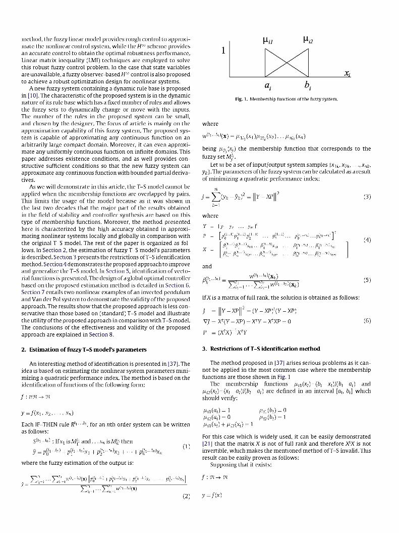
Fig. 1. Membership functions of tlie fuzzy system.

where

w('l^^'"'(x) = /Aii-,(Xi)/i2,2(X2). . . /Ani„(Xn)

being jijiiXj) the membership function that corresponds to the fuzzy set Mi.

Let m be a set of input/output system samples {Xn.,X2k x„i., yi(}. The parameters of the fuzzy system can be calculated as a result of minimizing a quadratic performance index:

(3) i - Z (yk-9k?' = ^"^^p k=l

where

y = lyi yi . . . ym f p = vV'vV'v'i--" . . . p < ' - " n(ri-rn) _p(ri-r„) 1

X = .../s';-"x„, .

/J(l-l)y . /3'n -•'"hnm

(4)

and

Pi il...in) . W(ll...ln)(x^)

If X is a matrix of full rank, the solution is obtained as follows:

J = \\Y -XP\\^ = (Y -XP)\Y -XP)

VJ = X^iY-XP)= X^Y - X^XP = 0

p = {x^xy^x^Y

(5)

(6)

2. Estimation of fuzzy T-S model's parameters 3. Restrictions of T-S identification method

An interesting method of identification is presented in [37]. The idea is based on estimating the nonlinear system parameters mini­mizing a quadratic performance index. The method is based on the identification of functions of the following form:

f :nm^m

y = / ( X i , X 2 , . . . , X n )

Each IF-THEN rule R'l '", for an nth order system can be written as follows:

S(ii...in) : ifxj isM'ji and ...Xn isMJf then

y = p(j'i ^ '") -I- p(j'i -^"hi + p? 'i '"'x2 H h PSI'I^ '"'xn

where the fuzzy estimation of the output is:

(1)

y ...y" w(ii-*)(x)

The method proposed in [37] arises serious problems as it can­not be applied in the most common case where the membership functions are those shown in Fig. 1

The membership functions m\{x{) = {bi-x{)\{bi-a{) and IM2iXi) = iXi-<ii)libi-ai) are defined in an interval [a,-, b,] which should verify:

/i„(a,-) = l tin{bi) = 0 /i,-2(a,-) = 0 fij2{bi) = '[

/An(Xi) + /Ai2(Xi) = l

For this case which is widely used, it can be easily demonstrated [21 ] that the matrix X is not of full rank and therefore X^X is not invertible, which makes the mentioned method of T-S invalid. This result can be easily proven as follows:

Supposing that it exists:

y^_^ • • • Er-i"""'-'"''{x) K'l"""'"' + p?i""*'xi + pp-'"''Xl +... + pgi-'«'x„l / : ^ -IH

(2) y=/ (x)

in which each row of the matrix X is of the form: 4. Proposed approach

Xk = ll^liXk) l^liXk)Xk l^liXk) ll2iXk)Xk

b - Xk b -Xk Xk-a Xk-a

b-a

verifying that:

-Xk Xk-~^Xk -j— Xk

(7)

b-Xk b-Xk Xk-T. ^Xk -r-

Xk--Xk

1

The rank of X in this case is 3. In other words, the columns of X are linearly dependent which in turn makes impossible the use of the above mentioned identification method proposed in [37]. Analyzing another example of two variables:

/ : 21H^1H

y = / ( x i , X 2 )

Each row of the matrix X is of the form:

[fM\fl2\ fM\fJa\Mk fM\fJa\^2k fJ'WfJ'll fJ'WfJ'llMk fM\fJa2^2k

fM2fJa\ fM2fJa\Mk fM2fJa\^2k fM2fJa2 Ml2M22^1fc Ml2M22^2fc] (8)

It can be noticed that the columns 1, 3, 4 and 6 have the same form as in the previous example multiplied by a constant jiw and therefore they are linearly dependent as well. The same thing hap­pens with the columns 6, 9,10 and 12, etc. In fact, the rank of the matrix in this case is 8.

The solution proposed in [37] avoids the occurrence of this sit­uation. In order to identify a function in the interval [a,-, b,] using T-S method, certain intermediate points are chosen of the form:

a? s [a,-, b,] andb? s [a,-, b,]

and they use membership functions which verify:

Xi - b? a,- < X < b*.

/ i „ (x )=<^ a , -b .?

0 b? < X < bi

0 Oj < X < a*.

IMiix) = { xi- a* a* < X < bi

(9)

(10)

bi - at

and thus:

/in(ai) = l tin{b*) = 0 lii2ia*) = 0 /i,-2(b,-) = l

which impedes that the domains of these functions being over­lapped and therefore it can be observed that, except for some isolated points,

and thus, in general, the matrixX will be of full rank and the method is applicable. This solution can be clearly seen in [37] where the authors find the optimum membership functions minimizing the performance index and reducing the problem to a nonlinear pro­gramming one. For this reason, they use the well-known complex method for the minimization. This can obviously be observed in the illustrative examples selected by the authors in [37] where all the identified memberships are non overlapping ones.

The restriction of T-S identification method for the case pre­sented in the previous section does not mean the non-existence of solutions rather than an incentive for their search. As it has been seen, the problem comes from the fact that the solution should fulfil:

y/=X^Y-X^XP = 0 (11)

But as it was shown above, the columns of the matrix X are lin­early dependent and consequently X' X is not an invertible matrix, therefore it is impossible to calculate P through:

P = [X^xy^X^Y (12)

Nevertheless, as the rows ofX' are linearly dependent, the indepen­dent term in Eq. (11) X' Ywill have the same dependence among its rows and thereupon the rank of the system matrix will be the same as the rank of the extended matrix with the independent term.

rank(X^X) = rank(X^X|X^Y)

And so the system has solution. In other words, the system is a compatible indeterminate one, that is, if P is a solution of (11) and K belongs to the kernel ofX' X

K e KeriX^X)

thenP* =P+/<'will also be a solution. Therefore, the problem is not the lack of a solution rather the existence of infinite solutions and the key idea is the ability to find one of them. Several proposals can be made to select a solution. In our case, the aim is to find solutions with lower norm.

4.1. Parameters' weighting method

An effective approach with few computational efforts, based on the well known parameters' weighting method, is proposed. The main target is to improve the choice of the performance index and minimize it. It is characterized by extending the objective function by including a weighting y of the norm of P vector.

J = j:Uyk-yk? + y'J2pf

\Y-XP\\ -^y^\\P\

This can be rewritten as follows:

(13)

Y-XP

Y

0

Ya-XaP

-^y \\P\\

X- 2 P

|2

(14)

Now the extended matrix Xa is of full rank, and the vector P can be computed as:

P = {XiXa)-'XiYa (15)

Obviously the solution that minimizes this index is not opti­mum. However, for a small value of)/, it will be close to the optimum one and it will be unique as well.

The weighting of y does not need to have a unique value, rather than some values can be weighted more than others to choose the most suitable one.

k=\ j

| |Y-XP|P + \\rp\\^

r r i r x i _ p

|_oJ [i'\

(16)

where F is a diagonal matrix formed by the values y^ which should necessarily have a value other than zero to guarantee that the extended matrix is invertible.

4.2. Example

In the following example, we will compare the proposed method with the one proposed by T-S in [37]. A non-linear function will be proposed and the fuzzy models will be obtained assigning an interval [a,-, b,] for each variable x,-. In this interval, two fuzzy sets are defined whose membership functions are:

However, as demonstrated above, these membership functions cannot be used directly in the method of T-S, as the resulting matrix X would not be full rank.

In order to compare these methods, we use a factor 0 < a < 1, which determines two points within the interval. This means:

a- =bi-a{bi-ai)

b? = a,- + a{bj - a,-)

And so, we define two fuzzy sets whose membership functions are:

X,- - bt

IMlM=< ^-"l • " " ' (17)

/Ai2(x) -- (18)

which are those used with the direct method of T-S. As a measure of error for comparing these methods, the maximum of the absolute values of the errors is used, which is the same method applied by T-S in [37].

Example 4.1. Consider the following simple nonlinear system:

It is aimed to estimate this system:

y-- x e [ 0 , l ]

Let us suppose that we define in this interval two fuzzy sets with their corresponding membership functions as follows:

/ i j(x) = 1 - X

/ i2 (x)=X

The objective is to calculate the corresponding fuzzy model in an optimum form:

S : IfxisM} theny:

S2 : Ifx is M2 theny :

-•PI + P\X

•• PI + p\x (19)

In order to identify the nonlinear function, we take 6 points uni­formly distributed {0, 0.2, 0.4, 0.6, 0.8, 1} in the interval [0, 1]. In the original T-S method [37], The X matrix becomes:

1 0 0 0 0.8 0.16 0.2 0.04

0.6 0.24 0.4 0.16

0.4 0.24 0.6 0.36

0.2 0.16 0.8 0.64

0 0 1 1

Its rank is 3 (the condition number is 8.1154e +015). The X'X prod­uct has the following value:

2.2 0.4 0.8 0.4 •

0.4 0.1664 0.4 0.2336

X 'X= 0.8 0.4 2.2 1.8

0.4 0.2336 1.8 1.5664

whose determinant is 5.5707e - 017. Applying the proposed weighting of parameters approach for

various values of y to examine the trade-off between the accuracy of the identification of the model and the condition number, the following results are obtained:

For y = 0.1, the obtained fuzzy rules are:

S : IfxisM} theny =-0.004-0.3167X

S2 : IfxisM^ theny = 0.3392-h0.6559x (20)

The error between the original system and the identified fuzzy model is with an error of 0.0050.

For y = 0.01, the obtained fuzzy rules are:

(21) S : IfxisM} theny = -0.3332x

S2 : IfxisM^ theny = 0.3334-h0.66666x

The error between the original system and the identified fuzzy model is with an error of 5.141 Oe- 005.

For y = 0.001, the obtained fuzzy rules are:

S : IfxisM} theny = -0.3333x

S2 : IfxisM^ theny = 0.3333-h0.6667x (22)

The error between the original system and the identified fuzzy model is with an error of 5.1409e - 007.

As it can be seen that although it is not an optimal solution, but it is obviously very close and presents a good estimation. In addition to that, it can be clearly noticed that as y is reduced, the accuracy of the identified model is tangibly increased though the condition number of the matrix Xa is about 3.6608e + 003 which is excessively high. In other words, Xa is ill-conditioned and this leads to an unreliable results.

In the method of T-S, let us suppose that a = 0.7. The fuzzy model is:

S : IfxisM} theny =-0.0389-h0.5238x

S2 : IfxisM^ theny =-0.5151-h 01.4762X (23)

The identification error is 0.0201, which is higher than the one obtained in the proposed two methods. Increasing a = 0.8, the error is reduced to 0.0160, i.e., the identification is improved. With a = 0.9, the error becomes 0.0081, where the identification is again improved. The same occurs for a = 0.95 where the error is reduced to 0.0044. In other words, as the factor a is approaching unity the identification is improved, but it cannot reach the optimum which precisely occurs when a = 1. Since at this value, the matrixX is not of full rank and therefore the matrixXfX is not invertible. Even when a is approaching unity, the condition number of the matrixX starts increasing which indicates that XfX is approaching the singular­ity and therefore its inverse is no longer numerically reliable. For instance, when a = 0.999, the condition number ofXis 5.2523e + 004 which shows clearly a non reliable result.

4.3. Parameters tuning using the parameters' weighting method

The parameters' weighting method can also be used for param­eters tuning of T-S model from local parameters obtained through the identification of a system in an operating region or from any physical input/output data.

We suppose that in this case we have a first estimation

Po- [Po Pi Ppl. •P°n\'

of the T-S model parameters. In order to obtain such an estimation, the classical least square method can be used around the equilib­rium point. The objective is to obtain a global approximation of the system.

y = Po + P°M + P2X2 + •••+ P°Xn

Let us analyze a set of input/output system samples {Xn.,X2fc Xnk<yk}- The parameters of the global approximation can be calcu­lated by minimizing the following quadratic performance index:

This first approximation can be utilized as reference parameters for all the subsystems. Then, the parameters' vector of the fuzzy model can be obtained minimizing:

J m T\

i i = i k=\

\\Y -Xp

Y

ypo

\Ya-Xap\

in = l J = 0

. p( i l ^ ) ) 2

+ riiPo-

X (27)

where

Po = [Po P0...P0]

In this case, the factor y represents the degree of confidence of the parameters initially estimated. In a similar way to the previous case, different weight factors of )/('i '") can be used to each one of the parameters p j ' i ' " ' depending on the reliability of the initial parameter p° in the specific rule.

m r-i

k=\ i i = l i n= l J = 0

n(ii ^ ) l 2 O

-xp|| ' + | | r (po-p) | | '

r Y

[^Po. -

"X"

r p

(28)

= | |ya-Xap||

where F is a diagonal matrix with the weight factor yf'i '"). It is not necessary to apply this process for all the parameters. If the values of some of them are known, they can be fixed beforehand or we can assign them a weighting factor yf'i '"' comparatively high.

5. Identification of vectorial functions

iyk-ykT = p-^sM (24) In the case of vectorial functions,

/ : IH" ^ IH™

where

Y =

Po =

\y\ yi y3 •

[pg P? P^ •

1 x i i X21

1 X\2 X22

1 Xln Xjn

ym\

pS!f

• • Xnl (25)

In this case, if we select a sufficient number of points distributed in the region where it is required to obtain the approximation, then the matrix Xg will be of a full rank and therefore, the solution becomes unique, which can be calculated as follows:

Po = (XjXg)-^XjY (26)

y=/ (x i ,X2, . . . ,Xn) yslH™

This function is equivalent to m scalar functions

yj=fj{xi,X2,... ,Xn) yslH, j = l , , , m

Each one of these functions can be modeled as follows:

5(ii i„) . ifxj isM'i andx2 isM'2 and .. .Xn isM'" then yj = p(h ^ in) + pj<l ^ ) x i + p<M ^ ) x 2 + ••• + p<h ^^'n)xn

Applying the previous method for each one of these models, we get in basic case:

(29)

^ . - [ Pi =

X =

yji yj2

„ ( i - i ) „ ( i - i )

yjN

n ( r i - -m) r ) ( r i - m ) )(ri--m) 1 J" J '-,0 '-'n '-in ' JO ''n

/ ! j ; - " / ! j ; - " x „ . . . / ! ] ; - " x „ , . . . /!(;i --«> /!(;i --«)x„ . . . /!(ji --«)x„,

and the formulation for parameters tuning becomes

(30)

l^iPjO. - Pj (31)

It is quite usual in the modelling of T-S model, that the fuzzy sets of the premise part of all the subsystems are the same, fulfilling in this case that:

Xi =X2 = Xm = X

In addition to that, if the weight factors yf'i '"' of the matrix F are the same for all the subsystems, they can be all grouped as follows:

J = Vl Y2 Ym

T p i o rp20 rpmO. -

X

r = Ya-XaPp

and the solution is still:

P = (X^^ a) X(j Ya

[P\ P2 Pm] (32)

(33)

6. Design of an optimal controller

In order to show the effectiveness of the proposed estimation methods, a design of an optimal controller is carried out for a dynamic system whose discrete model is following:

x{k + \)=f{x{k),u{k)) xenm uemm

Applying the proposed estimation method mentioned above to a set of points, the T-S model can be adjusted as follows:

S(ii--*) : lfx,(;<)isM'i andX2(/<)isM^2and... andx„(/<)isM*>

thenx(/< + 1) = a'n-in) +A'n-''^'ix(k) + B('i-'n'u(/<) (34)

a 'i ^ '"' s nm A 'i ^ '"' enxnm ' ( i l^^^in) mlH

where M51 (I'l =1,2 ri) are fuzzy sets for Xi(/c),M^2 (12 = 1,2 r2) are fuzzy sets for X2(fe) and MJf (in = 1, 2 Tn) are fuzzy sets forXn(fe). The fuzzy system is described as:

V" ' . . . V ' ° w('i-*'(x(;<)) [a(;i-*'+/i('i-'«'x(;<)l

J2'^_j • • • J27-,^^'^ -'«'(x(;<)) |B('i -'«)u(;<)]

which is equivalent to the system:

x{k + 1) = ao{x{k)) +A{x{kMk) + B{x{k))u{k)

(35)

(36)

a time interval, minimizing a quadratic performance index of the form:

k i - i

J = ^x\k + 1 )Q_xik + 1) + u\k)Ruik) (38) k=ko

Q. is a non-negative definite matrix which is called weighting matrix. On the other hand, R is a positive definite weighting matrix. Optimal selection of these matrices determines the dynamic speed of the controller as well as amplitudes of state variables and control signals. For example if R is selected small while Q. is selected large, more stability will be attained with large control efforts.

The solution is well known [2-4,27,49] when the system is a linear one. However, it is not easy enough for the nonlinear system obtained before (see Eq. (36). In order to solve this problem, it is proposed to minimize the cost of each step instead of the global cost. The solution will be a suboptimal one but with a great advan­tage due to its easy calculation. It is suggested in each step to apply the control action that minimizes:

Jfc = x'{k + 1 )Qx{k +-[) + u'{k)Ru{k) (39)

Substituting (36) in (39), we obtain:

Jk = lao{x{k))+A{x{k))x{k) + B{x{k))u{k)]'

X a[ao(x(/<)) + A{x{k))x{k) + B{x{k))u{k)] + u'{k)Ru{k) (40)

Applying the gradient and equating to zero to minimize the perfor­mance index:

V„(k)/k = 2[aoixik))+Aixik))xik) + Bixik)Mk)]'

X QBixik)) + 2u^ik)R = 0

Thus,

Ru{k) + B'{x{k))(llao{x{k)) +A{x{k))x{k) + B{x{k))u{k)] = B'{x{k))

xQ_[aoixik))+Aixik))xik)] + [R + B\xik))mxik))Mk) (41)

The optimal control law is then computed as follows:

u{k) = -[R + B'{x{k))QB{x{k))]-'B'{x{k)mao{x{k)) + A{x{k))x{k)]

where the matrices are determined by the fuzzy system as follows: 7. Illustrative example

S(ii--in) : Ifxi(/<)isMji andX2(/<)isM5!and... andx„(/<)isMj,n

then ao = agi --'»' and/I = ACi --'»' and B = Bd --'»' (37)

In order to calculate the rest of control coefficients, any control design methodology through state feedback control can be applied. However, these methodologies can lead to systems where the control action exceeds the allowed environment limits. Selecting closed loop poles with great negative real parts make the dynamic response of the system to be quick while the control effort to be greater than permissible levels. If selection of the closed loop poles saturate of control signals, dynamic behavior of the system will not be as same as the desired behavior even it may become unsta­ble. Therefore optimal selection of closed loop poles will lead to a trade-off between speed of dynamic response and control effort. Together with the proposed estimation method, the well known Linear Quadratic Regulator (LQR) method might be an appropri­ate choice. With this method we might not guarantee of stability, which needs to be analyzed a posteriori, gaining in return a balance between static and dynamic behavior of the system with admissible control actions.

The objective is to find the control action u(/c) to transfer the system from any initial state x(/co) to some final state x(/ci) = 0 in

In this section the proposed estimation method and its applica­tion to design a FC-LQR is illustrated by two examples of an inverted pendulum and Van der Pol oscillator respectively.

Example 7.1. Inverted pendulum:

Consider the problem of stabilizing and balancing of swing up of an inverted pendulum (see Fig. 2). The control of this system is a widely used performance measure of a controller, since this sys­tem is unstable and highly nonlinear. The objective is to maintain the inverted pendulum upright with 9 despite small disturbances due to wind or system noises. The inverted pendulum can be rep­resented as follows:

e--^ s i n 0 - c o s 6{{u + ml6'^ sin 6)/{M + m))

1(4/3-(mcos^e/M + m) (42)

where 9 denotes the angular position (in radians) deviated from the equilibrium position (vertical axis) of the pendulum and 9 is the angular velocity, g(gravityacceleration) = 9.8 m/s^, M (mass) of the cart = l kg, m (mass) of the pole = 0.1 kg, / is the distance from the center of the mass (m) of the pole to the cart = 0.5 m.

Centre of grcMty

Fig. 2. Inverted pendulum system.

•71/4 0 "^M X

Fig. 3. Membership functions fortlie angle x of the inverted pendulum.

Assuming that Xj =0 and X2 = 9, then (42) can be rewritten in state space form as follows:

xi =9

X2

.9 (43)

sin(xi) - cos(xi )((u + mlxj sin(xi ))/(M + m)) /(4/3 - (m cos2(xi )/(M + m))

The aim is to move the pendulum to its instable equilibrium position, i.e., Xj =X2 = 0. In order to control the system, a discrete controller is proposed with a sampling time of 0.1 s and a sample-hold device is used for the control action. It is suggested to model the equivalent discrete system as:

x{k + 1) = ao(x(/<)) +A{x{k))x{k) + B{x{k))u{k)

X s 21H us lH ao s 21H A s 2 x 21H B s 21H

(44)

Using the proposed methodology, supposing the universe of dis­course of the angle is {-njA, TCJA\ rad. and the one of the angular velocities is [-5, 5]rad/seg. Both membership functions for the angle x and its derivative x' are shown in Figs. 3 and 4 respectively.

-5 " 5 X

Fig. 4. Membership functions for the angular velocity of the inverted pendulum.

If we apply the T-S method directly to this example, then the condition number of the matrix X is 3.4148e + 015, which shows clearly a non reliable result.

By using the identification with the classical least square method in an interval close to the equilibrium point

Xi S - T T TT

l o " ' 4 0 X2 s [-0.5, 0.5]

The resultant linear model of the system in this interval is:

X{k + \): 1 . 0 7 9 0 0 . 1 0 2 6

1 . 6 1 5 4 1 . 0 7 8 8 x{k) +

- 0 . 0 0 7 3

- 0 . 1 4 9 9 u{k)

This approximation gives us an idea of the quantitative relation among various variables. By applying the tuning of parameters method, taking as a reference the parameters obtained through least square method with a weighting factor )/ = 0.001 *np, where np is the number of samples used in the identification, we obtain:

lf(xi isMj)and(X2 is M') then "1.0696 0.1010

x(;< + i) = 0.0037

0.0865 1.3784 1.0388

lf(xi isMj)and(X2 is M^) then

x(;< + i) = 0.0029

0.0610

1.0724 0.1022

1.4757 1.0665

lf(xi isMj)and(X2 is M^) then

x(;< + i) = 0.0034

0.0795

1.0786 0.1035

1.6547 1.0958

S21 : lf(x, isM2)and(X2isMi)then

x(;< + i) = 0.0001

0.0021

1.0831 0.1023

1.6833 1.0687

x(k) +

x(k) +

x(k) +

m +

-0.0041

-0.0707

-0.0053

-0.1074

-0.0062

-0.1361

-0.0075

-0.1499

uQi)

u(k)

u(,k)

u(,k)

lf(xi isM2)and(X2 is M^) then

x(;< + i) = -0 .0000

-0 .0000

1.0875 0.1028

1.7990 1.0861 x(k) +

-0.0078

-0.1599

S23 : If (x, is M2) and (X2 is M^) then

x(;< + i) = -0 .0000

-0.0006

1.0831 0.1022"

1.6833 1.0683

S i : lf(x, isM3)and(X2isMi)then

x(;< + i) = -0.0035

-0.0802

1.0786 0.1034"

1.6536 1.0954

S32 : If (x, is M^) and (X2 is M2 ) then

x(;< + i) = -0.0029

-0.0612

1.0724 0.1022

1.4756 1.0663

x(k) + • -0.0075

-0.1494

x(k) + " -0.0062

-0.1362

x(k) + • -0.0053

-0.1066

5 3 : If (x, is M^) and (X2 is M^) then

x(;< + i) = -0.0037

-0.0873

1.0696 0.1010

1.3774 1.0392 x(k) +

-0.0042

-0.0714

u(k)

u(k)

u(,k)

u(,k)

u(k)

which has a mean square error of 7.9608e - 006. It has been taken into account that the system has an instable equilibrium point in [0 0], therefore, it should fulfill that

. (2 .2) .

To achieve this target, we can either fix the value of this parameter or assign it a very large weighting factor as explained in Section (4.3). In this case, a weighting factor of lOOy has been assigned to this parameter.

For the control system, it is required to minimize the following performance index:

Jfc=X^(/< + l ) 1 0 0 0

0 1 xik + 'i) + u\k)[Om]uik)

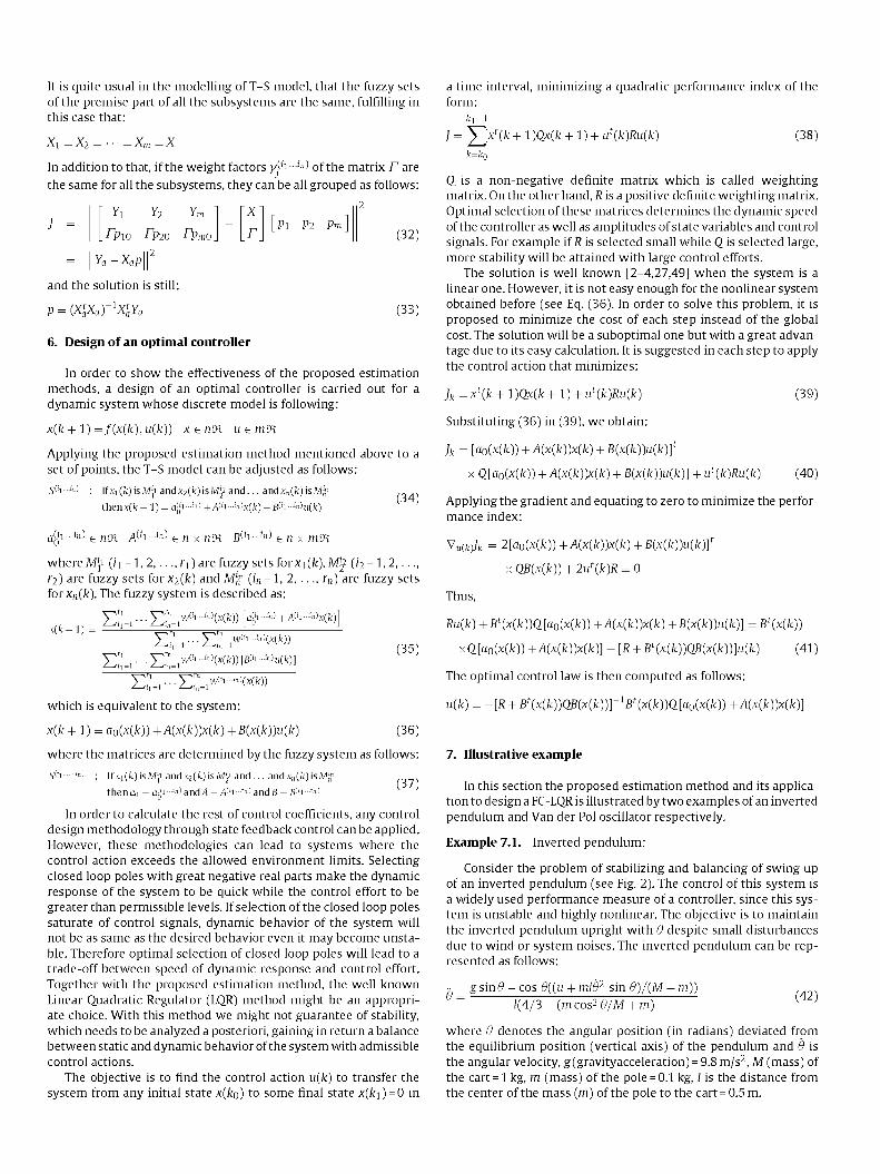
Fig. 5 shows the controlled system behavior subjected initial con­ditions [15°0]' and [-10°0]'^. Fig. 6 shows the controlled system

0 0.5 1 1.5 2 Time (seconds)

2.5

Fig. 5. Transient response of the inverted pendulum controlled by the fuzzy LQR.

15,

4 5 6 Time (seconds)

Fig. 6. Transient response of the inverted pendulum controlled by the fuzzy LQR subjected to disturbances.

-10 0 10

Angle(deg.)

Fig. 7. Trajectories of the system for several initial conditions.

Fig. 8. Membership functions for X.

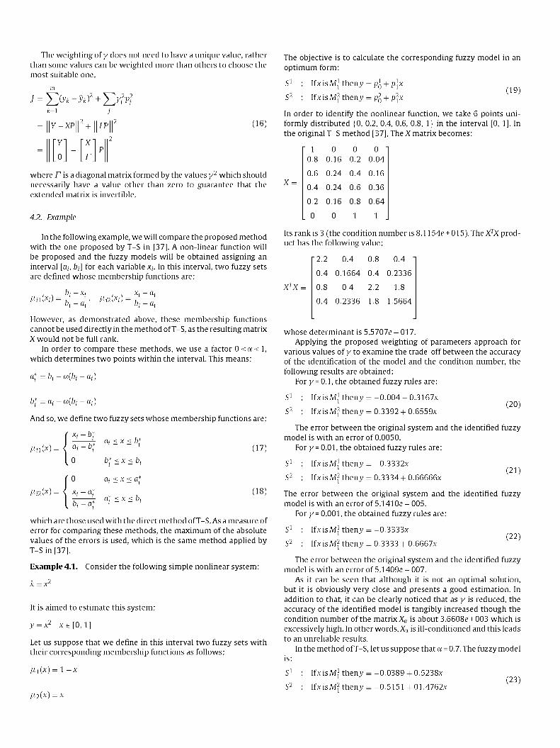
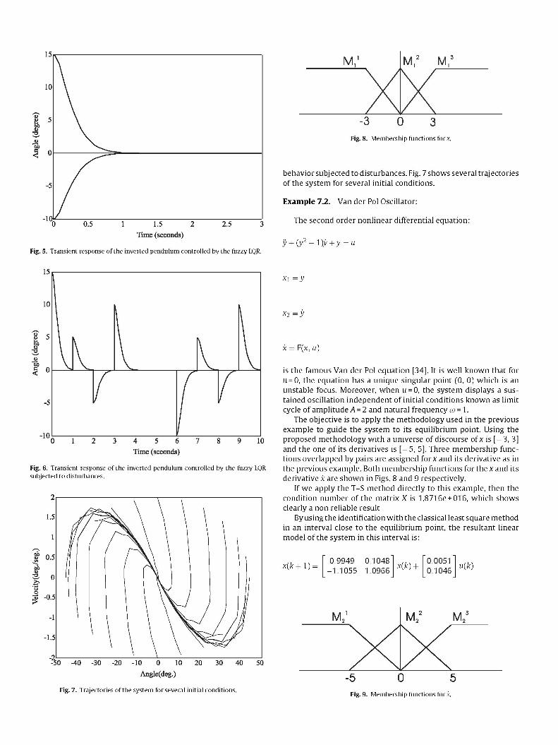
behavior subjected to disturbances. Fig. 7 shows several trajectories of the system for several initial conditions.

Example 7.2. Van der Pol Oscillator:

The second order nonlinear differential equation:

y + ( y ^ - i ) y + y = "

X2=y

X = F(x, u) is the famous Van der Pol equation [34]. It is well known that for u = 0, the equation has a unique singular point (0, 0) which is an unstable focus. Moreover, when u = 0, the system displays a sus­tained oscillation independent of initial conditions known as limit cycle of amplitude A = 2 and natural frequency (o=\.

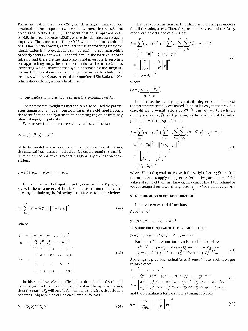
The objective is to apply the methodology used in the previous example to guide the system to its equilibrium point. Using the proposed methodology with a universe of discourse of x is [- 3, 3] and the one of its derivatives is [-5, 5]. Three membership func­tions overlapped by pairs are assigned forx and its derivative as in the previous example. Both membership functions for the x and its derivative x are shown in Figs. 8 and 9 respectively.

If we apply the T-S method directly to this example, then the condition number of the matrix X is 1.8716e + 016, which shows clearly a non reliable result

By using the identification with the classical least square method in an interval close to the equilibrium point, the resultant linear model of the system in this interval is:

X{k + \): 0.9949 -1.1055

0.1048 1.0966

x{k) + 0.0051 0.1046

u{k)

Fig. 9. Membership functions forx.

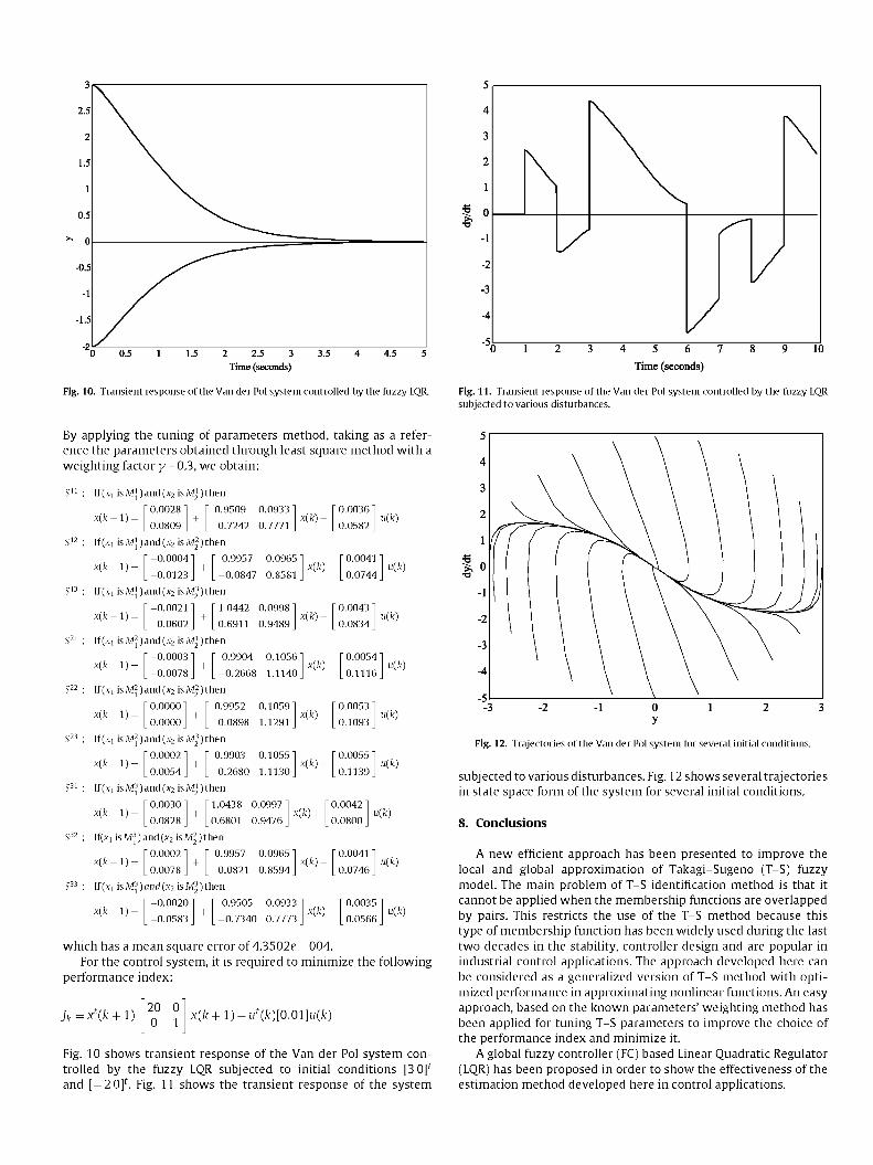
Fig. 10. Transient response of tlie Van der Pol system controlled by the fuzzy LQR.

Time (seconds)

Fig. 11. Transient response of the Van der Pol system controlled by the fuzzy LQR subjected to various disturbances.

\

\

/

/

0 1 2 5 4 5 5 7 i ? 10

By applying the tuning of parameters method, taking as a refer­ence the parameters obtained through least square method with a weighting factor )/ = 0.3, we obtain:

If (x, is M\) and (xj is M') then

x(;< + i) = 0.0028

0.0809

0.9509 0.0933

-0.7242 0.7771 x(k) +

0.0036

0.0582 u(k)

lf(xi isMj)and(X2 is M^) then

x(;< + i ) = -0.0004

-0.0123

0.9957 0.0965

-0.0847 0.8581 x(k) +

0.0041

0.0744 u(,k)

S " : lf(x, isMj)and(X2 is M^) then

x(;< + i) = -0.0021

-0.0602

1.0442 0.0998

0.6911 0.9489 x(k) +

0.0043

0.0834 u(,k)

S" : lf(x, isM2)and(X2isMi)then

x(;< + l) = -0.0003

-0.0078

0.9904 0.1056

-0.2668 1.1140 x(k) +

0.0054

0.1116 u(k)

S22 : If (x, is M2) and (X2 is M2) then

x(;< + i) = 0.0000

0.0000

0.9952 0.1059

-0.0898 1.1291

lf(xi isM2)and(X2 is M^) then

x(;< + i) = 0.0002

0.0054

0.9903 0.1055

-0.2680 1.1130

x(k) +

x(k) +

0.0053

0.1093

0.0055

0.1139

u(k)

u(,k)

S i : lf(x, isM3)and(X2isMi)then

x(;< + i) = 0.0030

0.0828

1.0438 0.0997

0.6801 0.9476 x(k) +

0.0042

0.0800 u(,k)

5 2 : lf(x, isM3)and(X2 isM^jthen

x(;< + i) = 0.0002

0.0078

0.9957 0.0965

-0.0821 0.8594 x(k) +

0.0041

0.0746 u(k)

S33 : lf(x, isM3)and(X2 isM^jthen

x(;< + l) = -0.0020

-0.0583

0.9505 0.0933

-0.7340 0.7773 x(k) +

0.0035

0.0566 u(k)

which has a mean square error of 4.3502e - 004. For the control system, it is required to minimize the following

performance index:

Jfc =/(/< + !) 20 0 0 1

x(/<+l) + u^(/<)[0.01]u(/<)

Fig. 10 shows transient response of the Van der Pol system con­trolled by the fuzzy LQR subjected to initial conditions [3 0] ^ and [-2 0]' . Fig. 11 shows the transient response of the system

- 3 - 2 - 1 0 1 2 3 y

Fig. 12. Trajectories of the Van der Pol system for several initial conditions.

subjected to various disturbances. Fig. 12 shows several trajectories in state space form of the system for several initial conditions.

8. Conclusions

A new efficient approach has been presented to improve the local and global approximation of Takagi-Sugeno (T-S) fuzzy model. The main problem of T-S identification method is that it cannot be applied when the membership functions are overlapped by pairs. This restricts the use of the T-S method because this type of membership function has been widely used during the last two decades in the stability, controller design and are popular in industrial control applications. The approach developed here can be considered as a generalized version of T-S method with opti­mized performance in approximating nonlinear functions. An easy approach, based on the known parameters' weighting method has been applied for tuning T-S parameters to improve the choice of the performance index and minimize it.

A global fuzzy controller (FC) based Linear Quadratic Regulator (LQR) has been proposed in order to show the effectiveness of the estimation method developed here in control applications.

Illustrative examples of an inverted pendulum and Van del Pol system have been chosen to evaluate the robustness and remark­able performance of the proposed method and the high accuracy obtained in approximating nonlinear and unstable systems locally and globally in comparison with the original T-S model. Simulation results have shown the potential, simplicity and generality of the algorithm. As future objectives, it is aimed to extend the proposed estimation method for multivariable nonlinear systems. The sec­ond target is to examine other control methodologies and compare them with the proposed LQR. It will also be an interesting issue to examine the validity of the proposed control method for tracking control problems for several typical reference inputs such as step, ramp, etc.

References

S. Alavandar, M.J. Nigam, Adaptive neuro-fuzzy inference system based control of six DOF robot manipulator,]. Eng. Sci.Technol. Rev. 1 (2008) 106-111. A.E. Bryson, Applied optimal control: optimization, estimation and control. Hemisphere (2008). B.D.O. Anderson, J.B. Moore, in: Optimal Control: Linear Quadratic Methods, Dover Publications, 2007. M. Athans, P. Falb, in: Optimal Control: An Introduction to the Theory and Its Applications, Dover Publications, 2006. P. Baranyi, SVD-based reduction to MISO TS models, IEEE Trans. Ind. Electron. 51 (February (1)) (2003) 232-242. S.G. Cao, N.W. Rees, G. Feng, Stability analysis of fuzzy control systems, IEEE Trans. Syst. Man Cybern. B Cybern. 26 (February (1)) (1996) 201-204. S.G. Cao, N.W. Rees, G. Feng, Analysis and design for a class of complex con­trol systems - Part I: fuzzy modeling and identification, Automatica 33 (1997) 1017-1028. B. Chen, Xiaoping Liu, Shaocheng Tong, Adaptive fuzzy output tracking control of MIMO nonlinear uncertain systems, IEEE Trans. Fuzzy Syst. 15 (April (2)) (2007) 287-300. B.-S. Chen, C-S. Tseng, H.-J. Uang, Robustness design of nonlinear dynamic sys­tems via fuzzy linear control, IEEE Trans. Fuzzy Syst. 7 (October (5)) (1999) 571-585. W. Chen, M. Saif A novel fuzzy system with dynamic rule base, IEEE Trans. Fuzzy Syst. 13 (October (5)) (2005) 569-582. O. Cordon, F. Herrera, L. Magdalena, P. Villar, A genetic learning process for the scaling factors, granularity and contexts of the fuzzy rule-based system data base. Inform. Sci. 136 (2001) 85-107. C. Fanutzzi, R. Rovatti, On the approximation capabilities of the homogeneous Takagi-Sugeno model, in: in: Proc. 5th IEEE Int. Conf Fuzzy Systems, New Orleans, LA, 1996, pp. 1067-1072. F. Gang, A survey on analysis and design of model-based fuzzy control systems, IEEE Trans. Fuzzy Syst. 14 (October (5)) (2006) 676-697. T.M. Guerra, L Vermeiren, LMI-based relaxed nonquadratic stabilization condi­tions for nonlinear systems in the Takagi-Sugeno's form, Automatica 40 (2004) 823-829. Y. Hou, Jacek M. Zurada, W. Karwowski, W.S. Marras, K. Davis, Identification of key variables using fuzzy average with fuzzy cluster distribution, IEEE Trans. Fuzzy Syst. 15 (August (4)) (2007) 673-685. T. Hseng, S. Li, S.-H. Tsai, Fuzzy bilinear model and fuzzy controller design for a classofnonlinearsystems, IEEE Trans. Fuzzy Syst. 15 (|une (3)) (2007) 494-506. T.P. Hong, C.Y. Lee, Induction of fuzzy rules and membership functions from training examples. Fuzzy Sets Syst. 84 (1) (1996) 33-47. K. Jae-Hun, C.-H. Hyun, E. Kim, M. Park, New adaptive synchronization of uncer­tain chaotic systems based on T-S fuzzy model, IEEE Trans. Fuzzy Syst. 15 (June (3)) (2007) 359-369. J.S.R.Jang,ANFIS: adaptive-network-based fuzzy inference systems, IEEE Trans. Syst. Man Cybern. 23 (03) (1993) 665-685. X. Jiang, Q.-L Han, Robust H control foruncertainTakagi-Sugeno fuzzy systems with interval time-varying delay, IEEE Trans. Fuzzy Syst. 15 (April (2)) (2007) 321-331.

121

|22

123

124

125

126

|27

|28

129

|30

131

|32

|33

134 135

|36

|37

|39

|39

140

141

142

143

144

145

146

147

|48

149

A. Jimnez, B.M. Al-Hadithi, F. Mata, An optimal T-S model for the estimation and identification of nonlinear functions, WSEAS Trans. Syst. Control October (3) (10) (2008) 897-906. T.A.Johansen, R. Shorten, R. Murray-Smith, On the interpretation and identifi­cation of dynamic Takagi-Sugeno models, IEEE Trans. Fuzzy Syst. 8 (|une (3)) (2000)297-313. J. Kim, Y. Suga, S. Won, A new approach to fuzzy modeling of nonlinear dynamic systems with noise: relevance vector learning mechanism, IEEE Trans. Fuzzy Syst. 14 (April (2)) (2006) 222-231. F. Klawonn, R. Kruse, Constructing a fuzzy controller from data. Fuzzy Sets Syst. 85(2)(1997) 177-193. M. Kumar, R. Stoll, N. Stoll, A min-max approach to fuzzy clustering, estimation, and identification, IEEE Trans. Fuzzy Syst. 14 (April (2)) (2006) 248-262. R. Langari, L Wang, Complex systems modeling via fuzzy logic, IEEE Trans. Syst. Man Cybern. B Cybern. 26 (February) (1996) 100-106. F.L. Lewis, in: Optimal and Robust Estimation: With An Introduction to Strochastic Control Theory, CRC Press, 2008. K.-Y. Lian, C.-H. Su, C-S. Huang, Performance enhancement forT-S fuzzy control usingneuralnetworks,IEEETrans. Fuzzy Syst. 14 (October (5)) (2006) 619-627. A. Mencattini, M. Salmeri, A. Salsano, Sufficient conditions to impose derivative constraints on MISO Takagi-Sugeno fuzzy logic systems, lEEETrans. Fuzzy Syst. 13 (August (4)) (2005). S. Mollov, R. Babuska, J. Abonyi, H.B. Verbruggen, Effective optimization for fuzzy model predictive control, lEEETrans. Fuzzy Syst. 12 (October (5)) (2004) 661-675. 0. Nelles, in: Nonlinear System Identification, Springer, Berlin, 2001, ISBN: 3540673695. K. Nozaki, H. Ishibuchi, H. Tanaka, A simple but powerful heuristic method for generating fuzzy rules from numerical data. Fuzzy Sets Syst. 86 (3) (1997) 251-270. 1. Skrjanc, S. Blazic, O. Agamennoni, Interval fuzzy model identification using l-norm, IEEE Trans. Fuzzy Syst. 13 (October (5)) (2005). J.-J.E. Slotine, in: Applied Nonlinear Systems, Prentice-Hall, 1991. M. Sugeno, G. Kang, Structure identification of fuzzy model. Fuzzy Sets Syst. 28 (1988) 15-33. M. Sugeno, K. Tanaka, Successive identification of a fuzzy model and its applications to prediction of a complex system. Fuzzy Sets Syst. 42 (1991) 315-334. T. Takagi, M. Sugeno, Fuzzy identification of systems and its applications to modeling and control, IEEE Trans. Syst. Man Cybern. SMC-15 (January (1)) (1985)116-132. K. Tanaka, T. Hori, H.O. Wang, A multiple Lyapunov function approach to stabi­lization of fuzzy control systems, IEEE Trans. Fuzzy Syst. 11 (August (4)) (2003) 582-589. K. Tanaka, H.O. Wang, in: Fuzzy Control Systems Design and Analysis: A Linear Matrix Inequality Approach, Wiley, New York, 2001. M.C.M. Teixeira, E. Assuno, R.G. Avellar, On relaxed LMI based designs for fuzzy regulators and fuzzy observers, IEEE Trans. Fuzzy Syst. 11 (October (5)) (2003) 613-623. L Wang, in: Adaptive Fuzzy Systems and Control: Design and Stability Analysis, Prentice-Hall, Englewood Cliffs, NJ, 1994, pp. 27-28. LX. Wang, J.M. Mendel, Design and analysis of fuzzy identifiers of nonlinear dynamic systems, IEEE Trans. Automat. Control 40 (January) (1995) 11-23. LX. Wang, J.M. Mendel, Generating fuzzy rules by learning from examples, IEEE Trans. Syst. Man Cybern. 22 (1992) 1414-1427. P. Xian-Tu, Generating rules for fuzzy logic controllers by functions. Fuzzy Sets Syst. 36 (1990) 83-89. Y. Yam, P. Baranyi, C.-T. Yangand, Reduction of fuzzy rule base via singular value decomposition, IEEE Trans. Fuzzy Syst. 712 (April (25)) (1999), 120-132675. H.Ying, General SISOTakagi-Sugeno fuzzy systems with linear rule consequent are universal approximators, IEEE Trans. Fuzzy Syst. 6 (November (4)) (1998) 582-587. W. Yu, X.O. Li, Fuzzy identification using fuzzy neural networks with stable learning algorithms, IEEE Trans. Fuzzy Syst. 12 Qune (3)) (2004) 411-420. K. Zeng, N.Y. Zhang, W.L. Xu, A comparative study on sufficient conditions for Takagi-Sugeno fuzzy systems as universal approximators, IEEE Trans. Fuzzy Syst. 8 (December (6)) (2000) 773-780. K. Zhou, in: Robust and Optimal Control, Prentice-Hall, 1996.