Mon. Not. R. Astron. Soc. 000, 000–000 (0000) Printed 16 May 2015 (MN L A T E X style file v2.2) A New Class of Accurate, Mesh-Free Hydrodynamic Simulation Methods Philip F. Hopkins 1 * 1 TAPIR, Mailcode 350-17, California Institute of Technology, Pasadena, CA 91125, USA Submitted to MNRAS, August, 2014 ABSTRACT We present two new Lagrangian methods for hydrodynamics, in a systematic comparison with moving-mesh, SPH, and stationary (non-moving) grid methods. The new methods are designed to simultaneously capture advan- tages of both smoothed-particle hydrodynamics (SPH) and grid-based/adaptive mesh refinement (AMR) schemes. They are based on a kernel discretization of the volume coupled to a high-order matrix gradient estimator and a Rie- mann solver acting over the volume “overlap.” We implement and test a parallel, second-order version of the method with self-gravity & cosmological integration, in the code GIZMO: 1 this maintains exact mass, energy and momentum conservation; exhibits superior angular momentum conservation compared to all other methods we study; does not require “artificial diffusion” terms; and allows the fluid elements to move with the flow so resolution is automatically adaptive. We consider a large suite of test problems, and find that on all problems the new methods appear com- petitive with moving-mesh schemes, with some advantages (particularly in angular momentum conservation), at the cost of enhanced noise. The new methods have many advantages vs. SPH: proper convergence, good capturing of fluid-mixing instabilities, dramatically reduced “particle noise” & numerical viscosity, more accurate sub-sonic flow evolution, & sharp shock-capturing. Advantages vs. non-moving meshes include: automatic adaptivity, dramatically reduced advection errors & numerical overmixing, velocity-independent errors, accurate coupling to gravity, good angular momentum conservation and elimination of “grid alignment” effects. We can, for example, follow hundreds of orbits of gaseous disks, while AMR and SPH methods break down in a few orbits. However, fixed meshes minimize “grid noise.” These differences are important for a range of astrophysical problems. Key words: methods: numerical — hydrodynamics — instabilities — turbulence — cosmology: theory 1 INTRODUCTION: THE CHALLENGE OF EXISTING NUMERICAL METHODS Numerical hydrodynamics is an essential tool of modern astro- physics, but poses many challenges. A variety of different numeri- cal methods are used, but to date, most hydrodynamic simulations in astrophysics (with some interesting exceptions) are based on one of two popular methods: smoothed-particle hydrodynamics (SPH; Lucy 1977; Gingold & Monaghan 1977), or stationary-grids, which can be either “fixed mesh” codes where a time-invariant mesh cov- ers the domain (e.g. Stone & Norman 1992), or “adaptive mesh refinement” (AMR) where the meshes are static and stationary ex- cept when new sub-cells are created or destroyed within parent cells (Berger & Colella 1989). These methods, as well as other more exotic schemes (e.g. Xu 1997; Zhang et al. 1997), have advantages and disadvantages. Unfortunately, even on simple test problems involving ideal fluid dynamics, they often give conflicting results. This limits their pre- dictive power: in many comparisons, it is unclear whether differ- ences seen owe to physical, or to purely numerical effects (for an example, see e.g. the comparison of cosmological galaxy formation in the Aquila project; Scannapieco et al. 2012). Unfortunately, both SPH and AMR have fundamental problems which make them inac- curate for certain problems – because of this, the “correct” answer is often unknown in these comparisons. In Table 1, we attempt a cursory summary of some of the methods being used in astrophysics today, making note of some * E-mail:[email protected]of the strengths and weaknesses of each. 1 Below, we describe these in more detail. 1.1 Smoothed-Particle Hydrodynamics (SPH) In SPH, quasi-Lagrangian mass elements are followed – the con- served quantities are discretized into particles (like an N-body code), and a kernel function is used to “smooth” their volumetric distributions to determine equations of motion. SPH is numerically stable, Lagrangian (follows the fluid), provides continuous adap- tive resolution, has truncation errors which are independent of the fluid velocity, couples trivially to N-body gravity schemes, exactly solves the particle continuity equation, and the equations of motion can be exactly derived from the particle Lagrangian (Springel & Hernquist 2002) giving it excellent conservation properties. 2 This has led to widespread application of SPH in many fields (for re- views see Rosswog 2009; Springel 2010; Price 2012b). However, it is well-known that “traditional” SPH algorithms 1 A public version of the GIZMO code (which couples the hydrodynamic algorithms described here to a heavily modified version of the paralleliza- tion and tree gravity solver of GADGET-3; Springel 2005) together with movies and additional figures, an extensive user’s guide, and the files and instructions needed to run the test problems in this paper, are available at http://www.tapir.caltech.edu/~phopkins/Site/ GIZMO.html 2 The “particle Lagrangian” and “particle continuity equation” are the La- grangian/continuity equation of a discretized particle field, where each par- ticle occupies an infinitely small volume. Exactly solving the continuity equation of a continuous fluid, of course, requires infinite resolution. This often leads to SPH being described as correct in the “molecular limit.” But at finite resolution, the more relevant limit is actually the “fluid limit.” c 0000 RAS
Transcript
Mon. Not. R. Astron. Soc. 000, 000–000 (0000) Printed 16 May 2015 (MN LATEX style file v2.2)
A New Class of Accurate, Mesh-Free Hydrodynamic SimulationMethodsPhilip F. Hopkins1∗
1TAPIR, Mailcode 350-17, California Institute of Technology, Pasadena, CA 91125, USA
Submitted to MNRAS, August, 2014
ABSTRACT
We present two new Lagrangian methods for hydrodynamics, in a systematic comparison with moving-mesh,SPH, and stationary (non-moving) grid methods. The new methods are designed to simultaneously capture advan-tages of both smoothed-particle hydrodynamics (SPH) and grid-based/adaptive mesh refinement (AMR) schemes.They are based on a kernel discretization of the volume coupled to a high-order matrix gradient estimator and a Rie-mann solver acting over the volume “overlap.” We implement and test a parallel, second-order version of the methodwith self-gravity & cosmological integration, in the code GIZMO:1 this maintains exact mass, energy and momentumconservation; exhibits superior angular momentum conservation compared to all other methods we study; does notrequire “artificial diffusion” terms; and allows the fluid elements to move with the flow so resolution is automaticallyadaptive. We consider a large suite of test problems, and find that on all problems the new methods appear com-petitive with moving-mesh schemes, with some advantages (particularly in angular momentum conservation), at thecost of enhanced noise. The new methods have many advantages vs. SPH: proper convergence, good capturing offluid-mixing instabilities, dramatically reduced “particle noise” & numerical viscosity, more accurate sub-sonic flowevolution, & sharp shock-capturing. Advantages vs. non-moving meshes include: automatic adaptivity, dramaticallyreduced advection errors & numerical overmixing, velocity-independent errors, accurate coupling to gravity, goodangular momentum conservation and elimination of “grid alignment” effects. We can, for example, follow hundredsof orbits of gaseous disks, while AMR and SPH methods break down in a few orbits. However, fixed meshes minimize“grid noise.” These differences are important for a range of astrophysical problems.
1 INTRODUCTION: THE CHALLENGE OF EXISTINGNUMERICAL METHODS
Numerical hydrodynamics is an essential tool of modern astro-physics, but poses many challenges. A variety of different numeri-cal methods are used, but to date, most hydrodynamic simulationsin astrophysics (with some interesting exceptions) are based on oneof two popular methods: smoothed-particle hydrodynamics (SPH;Lucy 1977; Gingold & Monaghan 1977), or stationary-grids, whichcan be either “fixed mesh” codes where a time-invariant mesh cov-ers the domain (e.g. Stone & Norman 1992), or “adaptive meshrefinement” (AMR) where the meshes are static and stationary ex-cept when new sub-cells are created or destroyed within parent cells(Berger & Colella 1989).
These methods, as well as other more exotic schemes (e.g.Xu 1997; Zhang et al. 1997), have advantages and disadvantages.Unfortunately, even on simple test problems involving ideal fluiddynamics, they often give conflicting results. This limits their pre-dictive power: in many comparisons, it is unclear whether differ-ences seen owe to physical, or to purely numerical effects (for anexample, see e.g. the comparison of cosmological galaxy formationin the Aquila project; Scannapieco et al. 2012). Unfortunately, bothSPH and AMR have fundamental problems which make them inac-curate for certain problems – because of this, the “correct” answeris often unknown in these comparisons.
In Table 1, we attempt a cursory summary of some of themethods being used in astrophysics today, making note of some
of the strengths and weaknesses of each.1 Below, we describe thesein more detail.
1.1 Smoothed-Particle Hydrodynamics (SPH)
In SPH, quasi-Lagrangian mass elements are followed – the con-served quantities are discretized into particles (like an N-bodycode), and a kernel function is used to “smooth” their volumetricdistributions to determine equations of motion. SPH is numericallystable, Lagrangian (follows the fluid), provides continuous adap-tive resolution, has truncation errors which are independent of thefluid velocity, couples trivially to N-body gravity schemes, exactlysolves the particle continuity equation, and the equations of motioncan be exactly derived from the particle Lagrangian (Springel &Hernquist 2002) giving it excellent conservation properties.2 Thishas led to widespread application of SPH in many fields (for re-views see Rosswog 2009; Springel 2010; Price 2012b).
However, it is well-known that “traditional” SPH algorithms
1 A public version of the GIZMO code (which couples the hydrodynamicalgorithms described here to a heavily modified version of the paralleliza-tion and tree gravity solver of GADGET-3; Springel 2005) together withmovies and additional figures, an extensive user’s guide, and the files andinstructions needed to run the test problems in this paper, are available athttp://www.tapir.caltech.edu/~phopkins/Site/GIZMO.html2 The “particle Lagrangian” and “particle continuity equation” are the La-grangian/continuity equation of a discretized particle field, where each par-ticle occupies an infinitely small volume. Exactly solving the continuityequation of a continuous fluid, of course, requires infinite resolution. Thisoften leads to SPH being described as correct in the “molecular limit.” Butat finite resolution, the more relevant limit is actually the “fluid limit.”
have a number of problems. They suppress certain fluid mixing in-stabilities (e.g. Kelvin-Helmholtz instabilities; Morris 1996; Dilts1999; Ritchie & Thomas 2001; Marri & White 2003; Okamotoet al. 2003; Agertz et al. 2007), corrupt sub-sonic (pressure-dominated) turbulence (Kitsionas et al. 2009; Price & Federrath2010; Bauer & Springel 2012; Sijacki et al. 2012), produce orders-of-magnitude higher numerical viscosity in flows which should beinviscid (leading to artificial angular momentum transfer; Cullen &Dehnen 2010), over-smooth shocks and discontinuities, introducenoise in smooth fields, and numerically converge very slowly.
The sources of these errors are known, however, and heroicefforts have been made to reduce them in “modern” SPH. First, theSPH equations of motion are inherently inviscid, so require someartificial viscosity to capture shocks and make the method stable;this generally leads to excessive diffusion (eliminating on of SPH’smain advantages). One improvement is to simply insert a Riemannsolver between particles (so-called “Godunov SPH”; see Inutsuka2002; Cha & Whitworth 2003), but this is not stable on many prob-lems; another improvement is to use higher-order switches (basedon the velocity gradients and their time derivatives) for the diffu-sion terms (Cullen & Dehnen 2010; Read & Hayfield 2012).
Second, a significant part of SPH’s suppression of fluid mixingcomes from a “surface-tension”-like error at contact discontinuitiesand free surfaces, which can be eliminated by kernel-smoothingall quantities (e.g. pressure), not just density, in the equations ofmotion (Ritchie & Thomas 2001; Saitoh & Makino 2013; Hopkins2013). Recently, it has also been realized that artificial diffusionterms should to be added for other quantities such as entropy (Price2008; Wadsley et al. 2008); and these further suppress errors atdiscontinuities by “smearing” them.
Third, and perhaps most fundamental, SPH suffers from low-order errors, in particular the so-called “E0” zeroth-order error(Morris 1996; Dilts 1999; Read et al. 2010). It is straightforwardto show that the discretized SPH equations are not consistent atany order, meaning they cannot correctly reproduce even a con-stant (zeroth-order) field, unless the particles obey exactly certainvery specific geometric arrangements. This produces noise, of-ten swamping real low-amplitude effects. Various “corrected” SPHmethods have been proposed which eliminate some of these errorsin the equation of motion (e.g. Morris 1996; Abel 2011; García-Senz et al. 2012): however, thus far all such methods require nu-merically unstable violations of energy and momentum conserva-tion, leading to exponentially growing errors in realistic problems(see e.g. Price 2012b). Adding terms to force them to be conserva-tive re-instates the original problem by violating consistency at ze-roth order, although it can still improve accuracy compared to otherchoices for the SPH equations of motion (García-Senz et al. 2012;Rosswog 2014). But in any case, these fixes also do not eliminateall the low-order inconsistencies. The only way to decrease all sucherrors is to increase the number of neighbors in the SPH kernel; us-ing higher-order kernels with several hundred neighbors, instead ofthe “traditional” ∼ 32 (Read et al. 2010; Dehnen & Aly 2012).3
3 It is sometimes said that “SPH does not converge,” or that “SPH is asecond-order method” (i.e. converges as N−2 in a smooth 1D problem).Both of these are incorrect. SPH does converge at second order, but only inthe limit where the number of neighbors inside the smoothing kernel goesto infinity (NNGB →∞), which eliminates the zeroth-order terms that donot converge away with increasing total particle number N alone. Howeverincreasing NNGB is both expensive and leads to a loss of resolution (and inmost actual practice is not actually done correctly as N increases). So thepractical convergence rates of SPH are very slow (see Zhu et al. 2014).
However, all of these improvements have costs. As such, it isunclear how “modern” SPH schemes compare with other methods.
1.2 Stationary-Grid Methods
In grid-based methods, the volume is discretized into points orcells, and the fluid equations are solved across these elements.These methods are well-developed, with decades of work in com-putational fluid dynamics. The most popular modern approach isembodied in finite-volume Godunov schemes,4 which offer higher-order consistency,5 numerical stability and relatively low diffusiv-ity, and conservation of mass, linear momentum, and energy.
However, there are errors in these methods as well. At fixedresolution, grid codes have much larger advection errors comparedto quasi-Lagrangian methods, when fluids (especially with sharpgradients) move across cells. These errors produce artificial diffu-sion, and can manifest as unphysical forces. For example, rotat-ing disks are “torqued” into alignment with the grid cardinal axes(“grid alignment”; see e.g. Hahn et al. 2010), shocks preferentiallyheat, propagate along, and “break out of” the grid axes (“carbun-cle” instabilities; Peery & Imlay 1988), and contact discontinuitiesare “smeared out” upon advection. Related to this, angular mo-mentum is not conserved: at realistic resolutions for many prob-lems, gaseous orbits can be degraded within a couple orbital times(unless special coordinates are used, which is only possible if theproblem geometry is known ahead of time). The errors in thesemethods are also velocity-dependent: unlike SPH, “boosting” thefluid (so it uniformly moves across the grid) increases diffusionacross the problem (see Wadsley et al. 2008; Tasker & Bryan 2008;Springel 2010) and suppresses fluid mixing instabilities (Springel2010). Grid methods also require special fixes (e.g. energy-entropyswitches; Ryu et al. 1993; Bryan et al. 1995) to deal with highlysuper-sonic flows. Free surfaces and steep “edges” (e.g. water flowin air, or sharp surfaces of planets/stars) require extremely highresolution to maintain. The inherent mis-match between particle-based N-body methods and cell-based hydro methods means thatvarious errors appear when the hydrodynamics are coupled to grav-ity, making it difficult for such methods to handle simple situationslike self-gravitating hydrostatic equilibrium (see Müller & Stein-metz 1995; LeVeque 1998; Zingale et al. 2002). Worse, these errorscan introduce spurious instabilities (Truelove et al. 1997, 1998).
In AMR methods, the fact that refinement boundaries arenecessarily dis-continuous entails a significant loss of accuracy atthe boundaries (the method becomes effectively lower-order). Thismeans convergence is slower. When coupled to gravity, variousstudies have shown these errors suppress low-amplitude gravita-tional instabilities (e.g. those that seed cosmological structure for-mation), and violate conservation in the long-range forces when-
4 Older, finite-difference methods simply discretized the relevant equationsonto interpolation points in a lattice, but these methods often do not con-serve quantities like mass, momentum, and energy, require artificial vis-cosity/diffusion/hyperviscosity terms (as in SPH), and can be numericallyunstable under long integrations for sufficiently complicated problems. Assuch they have proven useful mostly for weak linear-regime flows wherestrong shocks are absent and growth of e.g. momentum errors will not cor-rupt the entire domain; here there can be significant advantages from thefact that such methods very easily generalize to higher-order.5 Typically second-order, or third-order in the case of PPM methods. Someschemes claim much higher-order; however, it is almost always the case thatthis is true only for a sub-set of the scheme (e.g. a gradient estimator). Inour convention, the order represents the convergence rate, which is limitedby the lowest-order aspect of the method.
ever cells are refined or de-refined (O’Shea et al. 2005; Heitmannet al. 2008; Springel 2010).
Again, significant effort has gone into attempts to reducethese sources of error. Higher-order WENO-type schemes for gra-dients can help reduce edge effects. Various authors have im-plemented partially-Lagrangian or “abitrary Lagrange-Eulerian”(ALE) schemes where partial distortion of the mesh is allowed,but then the meshes are re-mapped to regular meshes; or “patch”schemes in which sub-meshes are allowed to move, then mappedto larger “parent meshes” (see e.g. Gnedin 1995; Pen 1998; Trac &Pen 2004; Murphy & Burrows 2008). However, these approachesusually require foreknowledge of the exact problem geometry towork well. And the re-mapping is a diffusive operation, so some ofthe errors above are actually enhanced.
1.3 Moving, Unstructured Meshes
Recently, there has been a surge in interest in moving, unstructuredmesh methods. These methods are well-known in engineering (seee.g. Mavriplis 1997), and there have been earlier applications inastrophysics (e.g. Whitehurst 1995; Xu 1997), but recently consid-erable effort has gone into development of more flexible examples(Springel 2010; Duffell & MacFadyen 2011; Gaburov et al. 2012).These use a finite-volume Godunov method, but partition the vol-ume into non-regular cells using e.g. a Voronoi tessellation, andallow the cells to move and deform continuously.
In many ways, moving meshes capture the advantages of bothSPH and AMR codes: like SPH they can be Lagrangian and adaptresolution continuously, feature velocity-independent truncation er-rors, couple well to gravity, and avoid preferred directions, whilealso like AMR treat shocks, shear flows, and fluid instabilities withhigh accuracy and eliminate many sources of noise, low-order er-rors, and artificial diffusion terms.
However, such methods are new, and still need to be tested todetermine their advantages and disadvantages. It is by no meansobvious that they are optimal for all problems, nor that they arethe “best compromise” between Lagrangian (e.g. SPH) and Eule-rian (e.g. grid) methods. And there are problems the method doesnot resolve. Angular momentum is still not formally conserved inmoving meshes, and it is not obvious (if the cell shapes are suffi-ciently irregular) how much it improves on stationary-grid codes.“Mesh-deformation” and “reconnection” in which distortions to themesh lead to highly irregular cell shapes, is inevitable in compli-cated flows. This can lead to errors which effectively reduce theaccuracy and convergence of the method, and would eventuallycrash the code. This is dealt with by some “mesh regularization,”by which the cells are re-shaped or prevented from deforming (i.e.made “stiff” or resistant to deformations). But such regularizationobviously risks re-introducing some of the errors of stationary-gridmethods which the moving-mesh method tries to avoid (the limitof a sufficiently stiff grid is simply a fixed-grid code with a uni-form drift). And dis-continuous cell refinement/de-refinement or“re-connection” is inevitable when the fluid motion is complicated,introducing some of the same errors as in AMR.
1.4 Structure of This Paper
Given the above, the intent of this paper is two-fold.First, we will introduce and develop two new methods for
solving the equations of hydrodynamics which attempt to simulta-neously capture advantages of both Lagrangian and Eulerian meth-ods (§ 2). The methods build on recent developments in the fluiddynamics community, especially Lanson & Vila (2008a,b), but
have not generally been considered in astrophysics, except for re-cent efforts by Gaburov & Nitadori (2011). The methods move withthe flow in a Lagrangian manner, adapt resolution continuously,eliminate velocity-dependent truncation errors, couple simply to N-body gravity methods, have no preferred directions, do not requireartificial diffusion terms, capture shocks, shear flows, and fluid in-stabilities with high accuracy, and exhibit remarkably good angularmomentum conservation. We will show how these methods can beimplemented into GIZMO, a new (heavily modified) version of theflexible, parallel GADGET-3 code.6
Second, we will consider a systematic survey of a wide rangeof test problems (§ 4-5), comparing both new methods, moving-mesh, modern stationary-grid, and both “traditional” and “modern”SPH methods. This is intended not just to validate our new meth-ods, but also to test the existing major classes of numerical meth-ods on a wide range of problems, to assess some of their relativestrengths and weaknesses in different contexts.
2 A NEW NUMERICAL METHODOLOGY FORHYDRODYNAMICS
In the last two decades, there has been tremendous effort in thecomputer science, engineering, and fluid dynamics literature, di-rected towards the development of new mesh-free algorithms forhydrodynamics; but much of this has not been widely recognizedin astrophysics (see e.g. Hietel et al. 2000). Various authors havepointed out how matrix and least-squares methods can be used todefine consistent, higher-order gradient operators, and renormal-ization schemes can be used to eliminate the zeroth-order errors ofmethods like SPH (see e.g. Dilts 1999; Oñate et al. 1996; Kuhnert2003; Tiwari & Kuhnert 2003; Liu et al. 2005). Most of this haspropagated into astrophysics in the form of “corrected” SPH meth-ods, which partially-implement such methods as “fixes” to certainoperators (e.g. García-Senz et al. 2012; Rosswog 2014) or in finitepoint methods, which simply treat all points as finite difference-like interpolation points rather than assigning conserved quantities(Maron & Howes 2003; Maron et al. 2012). However these im-plementations often sacrifice conservation (of quantities like mass,momentum, and energy) and numerical stability. Meanwhile, otherauthors have realized that the uncertain and poorly-defined artifi-cial diffusion operators can be eliminated by appropriate solutionof a Riemann problem between particle faces; this has generallyappeared in the form of so-called “Godunov SPH” (Cha & Whit-worth 2003; Inutsuka 2002; Cha et al. 2010; Murante et al. 2011).However on its own this does not eliminate other low-order SPHerrors, and those errors can de-stabilize the solutions.
A particularly intriguing development was put forward byLanson & Vila (2008a,b). These authors showed that the advancesabove could be synthesized into a new, meshfree finite-volumemethod which is both consistent and fully conservative. This is afundamentally different method from any SPH “variant” above;it is much closer in spirit to moving-mesh methods. Critically,rather than just attaching individual fixes piece-wise to an existingmethod, they re-derived the discrete operators from a consistentmathematical basis. A first attempt to implement these methodsin an astrophysical context was presented in Gaburov & Nitadori
6 Detailed attribution of different algorithms in the code, and descriptionsof how routines originally written for GADGET-3 have been modified, canbe found in the public source code.
Adaptive-Mesh Refinement (AMR) 2-3 X × Riemann X ∼ 8−48 over-mixing,(ENZO, RAMSES, FLASH) (1) solver + ∼ 24−216 ang. mom., VDE,
slope-limiter refinement criteriaMoving-Mesh Methods 2 X × Riemann X ∼ 13−30 mesh deformation,(AREPO, TESS, FVMHD3D) solver + ang. mom. (?),
slope-limiter “mesh noise”
New Methods In This PaperMeshless Finite-Mass 2 X up to Riemann X ∼ 32 partition noise& Meshless Finite-Volume gradient solver + ?(MFM, MFV) errors slope-limiter (TBD)
A crude description of various numerical methods which are referenced throughout the text. Note that this list is necessarily incomplete, and specific sub-versionsof many codes listed have been developed which do not match the exact descriptions listed. They are only meant to broadly categorize methods and outlinecertain basic properties.(1) Method Name: Methods are grouped into broad categories. For each we give more specific sub-categories, with a few examples of commonly-used codes thiscategory is intended to describe.(2) Order: Order of consistency of the method, for smooth flows (zero means the method cannot reproduce a constant). “Corrected” SPH is first-order in thepressure force equation, but zeroth-order otherwise. Those with 2-3 listed depend on whether PPM methods are used for reconstruction (they are not 3rd order inall respects). Note that all the high-order methods become 1st-order at discontinuities (this includes refinement boundaries in AMR).(3) Conservative: States whether the method manifestly conserves mass, energy, and linear momentum (X), or is only conservative up to integration accuracy (×).(4) Angular Momentum: Describes the local angular momentum (AM) conservation properties, when the AM vector is unknown or not fixed in the simulation. Inthis regime, no method which is numerically stable exactly conserves local AM (even if global AM is conserved). Either the method has no AM conservation(×), or conserves AM up to certain errors, such as the artificial viscosity and gradient errors in SPH. If the AM vector is known and fixed (e.g. for test massesaround a single non-moving point-mass), it is always possible to construct a method (using cylindrical coordinates, explicitly advecting AM, etc.) which perfectlyconserves it.(5) Numerical Dissipation: Source of numerical dissipation in e.g. shocks. Either this comes from an up-wind/Riemann solver type scheme (where diffusioncomes primarily from the slope-limiting scheme; Toro et al. 2009), or artificial viscosity/conductivity/hyperdiffusion terms.(6) Integration Stability: States whether the method has long-term integration stability (i.e. errors do not grow unstably).(7) Number of Neighbors: Typical number of neighbors between which hydrodynamic interactions must be computed. For meshless methods this is the numberin the kernel. For mesh methods this can be either the number of faces (geometric) when a low-order method is used or a larger number representing the stencilfor higher-order methods.(8) Known Difficulties: Short summary of some known problems/errors common to the method. An incomplete and non-representative list! These are describedin actual detail in the text. “Velocity-dependence” (as well as comments about noise and lack of conservation) here refers to the property of the errors, not theconverged solutions. Any well-behaved code is conservative (of mass/energy/momentum/angular momentum), Galilean-invariant, noise-free, and captures thecorrect level of fluid mixing instabilities in the fully-converged (infinite-resolution) limit.
(2011),7 and the results there for both hydrodynamic and magneto-hydrodynamic test problems appeared extremely encouraging. Wetherefore explore and extend two closely-related versions of thismethod here.
2.1 Derivation of the Meshless Equations of Motion
We begin with a derivation of the discretized equations govern-ing the new numerical schemes. This will closely follow Gaburov& Nitadori (2011), and is aimed towards practical aspects of im-plementation. A fully rigorous mathematical formulation of themethod, with proofs of various consistency, conservation, andconvergence theorems, is presented in Lanson & Vila (2008a,b);Ivanova et al. (2013).
The homogeneous Euler equations for hydrodynamics are ulti-mately a set of conservation laws for mass, momentum, and energy,which form a system of hyperbolic partial differential equations ina frame moving with velocity vframe of the form
∂U∂t
+∇· (F−vframe⊗U) = 0 (1)
where ∇·F refers to the inner product between the gradient oper-ator and tensor F, ⊗ is the outer product, U is the “state vector” ofconserved (in the absence of sources) variables,
U =
ρρvρe
=
ρρv
ρu + 12 ρ |v|
2
=
ρρvx
ρvy
ρvz
ρu + 12 ρ |v|
2
(2)
(where ρ is mass density, e is the total specific energy, u the specificinternal energy, and the last equality expands the compact form of vin 3 dimensions), and the tensor F is the flux of conserved variables
F =
ρvρv⊗v + PI(ρe + P)v
(3)
where P is the pressure, and I is the identity tensor.As in the usual Galerkin-type method, to deal with non-linear
and discontinuous flows we begin by determining the weak solutionto the conservation equation. We multiply Eq. 1 by a test functionφ, integrate over the domain Ω (in space such that dΩ = dνx, whereν is the number of spatial dimensions), and follow an integration byparts of the φ∇·F term to obtain:
0 =
∫Ω
(dUdtφ−F ·∇φ
)dΩ +
∫∂Ω
(Fφ) · n∂Ω d ∂Ω (4)
where d f/dt ≡ ∂ f/∂t + vframe(x, t) ·∇ f is the co-moving deriva-tive of any function f , and n∂Ω is the normal vector to the surface∂Ω. The test function φ = φ(x, t) is taken to be an arbitrary (dif-ferentiable) Lagrangian function (dφ/dt = 0). Assuming the fluxesand/or φ vanish at infinity, we can eliminate the boundary term andpull the time derivative outside of the integral (see Luo et al. 2008)to obtain
0 =ddt
∫Ω
U(x, t)φ dνx−∫
Ω
F(U, x, t) ·∇φ dνx (5)
To discretize this integral, we must now choose how to dis-cretize the domain volume onto a set of points/cells/particles i with
7 The source code from that study (WPMHD) is available athttps://github.com/egaburov/wpmhd/tree/orig
coordinates xi. If we chose to do so by partitioning the volume be-tween the xi with a Voronoi mesh, we would obtain the moving-mesh method of codes like AREPO with the more accurate gradientestimators implemented in Mocz et al. (2014). Here we consider amesh-free alternative, following Lanson & Vila (2008a,b); Gaburov& Nitadori (2011). Consider a differential volume dνx, at arbitrarycoordinates x; we can partition that differential volume fractionallyamong the nearest particles/cells8 through the use of a weightingfunction W , i.e. associate a fraction ψi(x) of the volume dνx withparticle i according to a function W (x−xi, h(x)):
ψi(x)≡ 1ω(x)
W (x−xi, h(x)) (6)
ω(x)≡∑
j
W (x−x j, h(x)) (7)
where h(x) is some “kernel size” that enters W . In other words,the weighting function determines how the volume at any pointx should be partitioned among the volumes “associated with” thetracer points i. Note that W can be, in principle, any arbitrary func-tion; the term ω(x)−1 normalizes the weights such that the total vol-ume always sums correctly (i.e. the sum of fractional weights mustalways be unity at every point). That said, to ensure the second-order accuracy of the method, conservation of linear and angularmomentum, and locality of the hydrodynamic operations, the func-tion W (x−xi, h(x)) must be continuous, have compact support (i.e.have W = 0 for sufficiently large |x−xi| h(x)), and be symmet-ric (i.e. depend only on the absolute value of the coordinate differ-ences |x− xi|, |y− yi|, etc.). Because of the normalization by ω(x),the absolute normalization of W is irrelevant; so without loss ofgenerality we take it (for convenience) to be normalized such that1 =
∫W (x−x′, h(x))dνx′.
An example of this is shown in Fig. 1, with (for comparison),the volume partitions used in moving-mesh and SPH methods. Weconstruct a two-dimensional periodic box of side-length unity withthree randomly placed particles, and use a cubic spline kernel forW with kernel length h set to the equivalent of what would contain≈ 32 neighbors in 3D. We confirm that the entire volume is indeedpartitioned correctly, like a Voronoi tessellation with the “edges”between particles smoothed (avoiding discontinuities in the “meshdeformation” as particles move9). In the limit where W is suffi-ciently sharply-peaked, we can see from Eq. 6 that we should re-cover exactly a Voronoi tessellation, because 100% of the weight(ψ(x)) will be associated with the nearest particle. In fact, techni-cally speaking, Voronoi-based moving-mesh methods are a specialcase of the method here, where the function W is taken to the limitof a delta function and the volume quadrature is evaluated exactly.10
8 In this paper, we will use the terms “particles” and “cells” interchange-ably when referring to our MFM and MFV methods, since each “particle”can just as well be thought of as a mesh-generating point which defines thevolume domain (or “cell”) whose mean fluid properties are represented bythe particle/cell-carried quantities.9 Throughout, when we refer to “mesh deformation,” we refer to the factthat when particles move, the volume partition – i.e. the map between posi-tion and association of a given volume element with different particles/cells– changes. This occurs constantly in Lagrangian codes (SPH/MFM/MFV,and moving meshes), regardless of whether or not the partition is explicitlyre-constructed each timestep or differentially “advected.”10 In practice, the reconstruction step (§ 2.4) differs slightly in mostVoronoi-mesh schemes, because they reconstruct the primitive quantities atthe centroid of the face, rather than at the point along the face intersectingthe line between the two points sharing said face.
Figure 1. Illustration of key conceptual differences between some of the methods here. For an irregularly distributed set of sampling/grid points or “particles”(black circles) with locations xi, we require a way to partition the volume to solve the equations of hydrodynamics between them. Left: The meshless finite-mass(MFM) and meshless finite-volume (MFV) methods here. The volume partition is given by the weighted kernel at each point (Eq. 6); here the red/green/bluecolor channels represent the fraction of the volume at each point associated with the corresponding particle (ψi(x)). Here we apply the same kernel function andtypical kernel “width” as in the text. Note that this returns a Voronoi tessellation with the boundaries “smoothed.” Despite the kernel function being spherical,the domains associated with each particle are not, and the entire volume is represented. The fluid equations are then solved by integrating over the domain ofeach particle/cell. Center: The unstructured/moving-mesh partition. Now the boundaries are strict step functions at the faces given by the tessellation. Notethat this is (exactly) the limit of our MFM/MFV method for an infinitely sharply-peaked kernel function; technically the moving-mesh method is a specialcase of the MFV method. The volume integrals are then reduced to surface integrals across the faces. Right: The SPH partition. In SPH the contribution tovolume integrals behaves as the kernel, centered on each particle location; the whole volume is “counted” only when the kernel size is infinitely large comparedto the inter-particle spacing (number of neighbors is infinite). The equations of motion are evaluated at the particle locations xi, using the weighted-averagevolumetric quantities from the volume partition.
We now insert this definition of the volume partition intoEq. 5, and Taylor-expand all terms to second order accuracy inthe kernel length h(x) (e.g. f (x) = fi(xi) + h(xi)∇ f (x = xi) ·(x− xi)/h(xi) +O(h(xi)
2); the algebra is somewhat tedious butstraightforward). Note that 1 =
∑i ψi(x), and since the kernel has
compact support, |x− xi| ∼ O(h(xi)) where W 6= 0. If we applythis to the integral of an arbitrary function (and assume the kernelfunction is continuous, symmetric, and compact) we obtain∫
f (x)dνx =∑
i
∫f (x)ψi(x)dνx (8)
=∑
i
fi(xi)
∫ψi dνx +O(hi(xi)
2) (9)
≡∑
i
fi Vi +O(h2i ) (10)
where Vi =∫ψi(x)dν x is the “effective volume” of particle i (i.e.
the integral of its volume partition over all of space). Applyingthe same to Eq. 5, evaluating the spatial integral, and dropping theO(h2) terms, we obtain
0 =ddt
∑i
Vi Uiφi−∑
i
Vi Fi · (∇φ)x=xi (11)
=∑
i
[φi
ddt
(Vi Ui)−Vi Fi · (∇φ)x=xi
]where Fi · (∇φ)x=xi refers to the product of the tensor F with thegradient of φ evaluated at xi.
To go further, and remain consistent, we require a second-order accurate discrete gradient estimator. Here, we can use locally-centered least-squares matrix gradient operators, which have beendescribed in many previous numerical studies (Dilts 1999; Oñateet al. 1996; Kuhnert 2003; Maron & Howes 2003; Maron et al.2012; Tiwari & Kuhnert 2003; Liu et al. 2005; Luo et al. 2008;
Lanson & Vila 2008a,b). Essentially, for any arbitrary configura-tion of points, we can use the weighted moments to defined a least-squares best-fit to the Taylor expansion of any fluid quantity at acentral point i, which amounts to a simple (small) matrix calcula-tion; the matrix can trivially be designed to give an arbitrarily high-order consistent result, meaning this method will, by construction,exactly reproduce polynomial functions across the particles/cells upto the desired order, independent of their spatial configuration. Thesecond-order accurate expression is:
(∇ f )αi =∑
j
β=ν∑β=1
( f j− fi)Bαβi (x j−xi)β ψ j(xi) +O(h2
i ) (12)
≡∑
j
( f j− fi) ψαj (xi)
ψαj (xi)≡β=ν∑β=1
Bαβi (x j−xi)β ψ j(xi)≡ Bαβi (x j−xi)
β ψ j(xi)
where the we assume an Einstein summation convention over theGreek indices α and β representing the elements of the relevantvectors/matrices, and the matrix Bi is evaluated at each i by takingthe inverse of another matrix Ei:
Bi ≡ E−1i (13)
Eαβi ≡∑
j
(x j−xi)α (x j−xi)
β ψ j(xi) (14)
Note that in Eqs. 12-14, we could replace the ψ j(xi) with any otherfunction ξ j(xi), so long as that function ξ is also continuous andcompact. However, it is computationally convenient, and physicallycorresponds to a volume-weighting convention in determining theleast-squares best-fit, to adopt ξ j(xi) = ψ j(xi), so we will followthis convention. It is straightforward to verify that when the f j fol-low a linear function in N-dimensions ( f j = fi +∇ ftrue · (x j−xi)),
this estimator exactly recovers the correct gradients (hence, themethod is consistent up to second order).
Now, inserting this into Eq. 11, and noting that:∑i
Vi Fαi (∇φ)αi =∑
i
∑j
Vi Fαi (φ j−φi) ψαj (xi) (15)
=−∑
i
φi
∑j
(Vi Fαi ψαj (xi)−Vj Fαj ψ
αi (x j))
we obtain
0 =∑
i
φi
( ddt
(Vi Ui) +∑
j
[Vi Fαi ψαj (xi)−Vj Fαj ψ
αi (x j)]
)(16)
This must hold for an arbitrary test function φ; so therefore theexpression inside the parenthesis must vanish, i.e.
ddt
(Vi Ui) +∑
j
[Vi Fαi ψαj (xi)−Vj Fαj ψ
αi (x j)] = 0 (17)
Now, rather than take the flux functions F directly at the par-ticle location and time of i or j, in which case the scheme wouldrequire some ad-hoc artificial dissipation terms (viscosity and con-ductivity) to be stable, we can replace the fluxes with the solutionof an appropriate time-centered Riemann problem between the par-ticles/cells i and j, which automatically includes the dissipationterms. We define the flux as Fi j; this replaces both Fi and F j sincethe solution is necessarily the same for both i and j “sides” of theproblem;11 this gives
ddt
(Vi Ui) +∑
j
Fαi j [Vi ψαj (xi)−Vj ψ
αi (x j)] = 0 (18)
Now, we can define the vector Ai j = |A|i j Ai j where Aαi j ≡Vi ψ
αj (xi)−Vj ψ
αi (x j), and the equations become:
ddt
(Vi Ui) +∑
j
Fi j ·Ai j = 0 (19)
This should be immediately recognizable as the form of theGodunov-type finite-volume equations. The term Vi Ui is simply theparticle-volume integrated value of the conserved quantity to becarried with particle i (e.g. the total mass mi = Vi ρi, momentum,or energy associated with the particle i); its time rate of change isgiven by the sum of the fluxes Fi j into/out of an “effective facearea” Ai j.
We note that our method is not, strictly, a traditional Godunovscheme as defined by some authors, since we do not actually calcu-late a geometric particle face and transform a volume integral intoa surface integral in deriving Eq. 19; rather, the “effective face”comes from solving the actual volume integral, over the partitiondefined by the weighting function, and this is simply the numericalquadrature rule that arises. But from this point onwards, it can betreated identically to Godunov-type schemes.
2.2 Conservation Properties
It should be immediately clear from Eq. 19, that since we ulti-mately calculate fluxes of conserved quantities directly between
11 Note that this replacement of Fi and F j can be directly derived, as well,by replacing the F in the integral Eq. 16 with a Taylor expansion in spaceand time, multiplying the terms inside by 1 =
∑ψi, centering the expansion
about the symmetric quadrature point between i and j and centering it atthe mid-point in time for a discretized time integral, and then evaluating theintegrals to second order. For details, see Lanson & Vila (2008a).
particles/cells, the conserved quantities themselves (total mass, lin-ear momentum, and energy) will be conserved to machine accu-racy independent of the time-step, integration accuracy, and parti-cle distribution. Moreover, it is trivial to verify that Ai j =−A ji, i.e.the fluxes are antisymmetric, so the flux “from i to j” is always thenegative of the flux “from j to i” at the same time, and the discreteequations are manifestly conservative.
2.3 Pathological Particle/Cell Configurations
We note that if very specific pathological particle configurations ap-pear (e.g. if all particles in the kernel “line up” perfectly), our gra-dient estimator (the matrix B in Eq. 12) becomes ill-conditioned.However it is straightforward to deal with this by expanding theneighbor search until cells are found in the perpendicular direction.Appendix C describes a simple, novel algorithm we use which re-solves these (very rare) special cases.
2.4 Solving the Discrete Equations
The approach to solving the discretized equations of the form inEq. 19 is well-studied; we can use essentially the same schemesused in grid-based Godunov methods. Specifically, we will em-ploy a second-order accurate (in space and time) MUSCL-Hancocktype scheme (van Leer 1984; Toro 1997), as used in state-of-the-art grid methods such as Teyssier (2002); Fromang et al. (2006);Mignone et al. (2007); Cunningham et al. (2009); Springel (2010).This involves a slope-limited, linear reconstruction of face-centeredquantities from each particle/cell, a first-order drift/predict step forevolution over half a timestep, and then the application of a Rie-mann solver to estimate the time-averaged inter-particle fluxes forthe timestep. Details of the procedure are given in Appendix A.
2.4.1 Gradient Estimation
In order to perform particle drift operations and reconstruct quan-tities for the Riemann problem, we require gradients. But we havealready defined an arbitrarily high-order method for obtaining gra-dients using the least-squares matrix method in Eq. 12-14. We willuse the second-order accurate version of this to define the gradi-ent of a quantity (∇ f )i at position xi; recall that these are exactfor linear gradients and always give the least-squares minimizinggradient in other situations. As noted by Mocz et al. (2014), thisgradient definition has a number advantages over the usual finite-volume definition (based on cell-to-cell differences).
2.4.2 Slope-Limiting in Mesh-Free Methods
However, as in all Riemann-problem based methods, some slope-limiting procedure is required to avoid numerical instabilities neardiscontinuities, where the reconstruction can “overshoot” or “un-dershoot” and create new extrema (see e.g. Barth & Jespersen1989). Therefore, in the reconstruction step (only), the gradient(∇ f )i above is replaced by an appropriately slope-limited gradi-ent (∇ f )lim, i, using the limiting procedure in Appendix B.
We have experimented with a number of standard slope-limiters like that in Gaburov & Nitadori (2011) and find generallysimilar, stable behavior. However, as noted by Mocz et al. (2014),for unstructured point configurations in discontinuous Galerkinmethods, there are some subtle improvements which can be ob-tained from more flexible slope-limiters. We find signifiant im-provement (albeit no major changes in the results here) if we adoptthe new, more flexible (and closer to total variation-diminishing)slope-limiting procedure described in Appendix B.
2.4.3 Reconstruction: Projection to the Effective Face
In Eq. 19, only the projection of the flux onto Ai j is required; there-fore the relevant flux Fi j · Ai j can be obtained by solving a one-dimensional, unsplit Riemann problem in the frame of the quadra-ture point between the two particles/cells. Because of the symmetryof the kernel, the relevant quadrature point at this order (the pointwhere the volume partition between the two particles is equal) isthe location along the line connecting the two which is an equalfraction of the kernel length h from each particle, i.e.
xi j ≡ xi +hi
hi + h j
(x j−xi
)(20)
This quadrature point moves with velocity vframe (at second order)
vframe, i j = vi + (v j−vi)[ (xi j−xi) · (x j−xi)
|x j−xi|2]
(21)
However, we note that we see very little difference in all thetest problems here using this or the first-order quadrature pointxi j = (xi + x j)/2 (which can sometimes be more stable, albeit lessaccurate).12.
So we must reconstruct the left and right states of the Rie-mann problem at this location: for a second-order method, we onlyrequire a linear reconstruction in primitive variables, so we requiregradients and reconstructions of the density ρ, pressure P (and in-ternal energy for a non-ideal equation of state), and velocity v. Foran interacting pair of particles i and j, the linearly-reconstructedvalue of a quantity f at a position x, reconstructed from the particlei, is frec, i = fi +(x−xi) · (∇ f )i and likewise for the reconstructionfrom particle j; these define the left and right states of the Rie-mann problem at the “interface” xi j. Details of the reconstructionand Riemann solver are given in Appendix A.
2.4.4 The Riemann Solver
Having obtained the left and right time-centered states, we thensolve the unsplit Riemann problem to obtain the fluxes Fi j. We haveexperimented with both an exact Riemann solver and the commonapproximate HLLC Riemann solver (Toro 1999); we see no differ-ences in any of the test problems here. So in this paper we adoptthe more flexible HLLC solver with Roe-averaged wave-speed es-timates as our “default” Riemann solver (see Appendix A).
2.4.5 Time Integration
The time integration scheme here closely follows that in Springel(2010), and additional details are given in Appendix G.
We use the fluxes Fi j to obtain single-stage second-order ac-curate time integration as in Colella (1990); Stone et al. (2008). Fora vector of conserved quantities Qi = (V U)i,
Q(n+1)i = Q(n)
i + ∆t⟨
dQi
dt
⟩≡Q(n)
i + ∆tdQi
dt
(n+1/2)
(22)
= Q(n)i −∆t
∑j
Ai j · F(n+1/2)i j (23)
12 As shown in Inutsuka (2002), a higher-order quadrature rule betweenparticles using the “traditional” SPH volume partition implies a quadraturepoint which is offset from the midpoint atO(h2). It is straightforward to de-rive an analogous rule here, and we have experimented with this. However,we find no significant improvement in accuracy, presumably because therest of the reconstruction we adopt is only second-order. Moreover, becauseInutsuka (2002) derive this assuming there is always an exact linear gra-dient connecting the particles and extrapolate this to infinity beyond them,this can lead to serious numerical instabilities in the Riemann problem whenthere is some particle disorder.
We employ a local Courant-Fridrisch-Levy (CFL) timestepcriterion; for consistency with previous work we define it as
∆tCFL, i = 2CCFLhi
|vsig, i|(24)
vsig, i = MAX j
[cs, i + cs, j−MIN
(0,
(vi−v j) · (xi−x j)
|xi−x j|
)](25)
where hi is the kernel length defined above, MAX j refers to themaximum over all interacting neighbors j of i, and |vsig| is the sig-nal velocity (Whitehurst 1995; Monaghan 1997b).13 We combinethis with a limiter based on Saitoh & Makino (2009) to preventneighboring particles/cells from having very different timesteps(see Appendix G).
We follow Springel (2010) to maintain manifest conserva-tion conservation of mass, momentum, and energy even whileusing adaptive (individual) timesteps (as opposed to a single,global timestep, which imposes a severe cost penalty on high-dynamic range problems). This amounts to discretizing timestepsinto a power-of-two hierarchy and always updating fluxes of con-served quantities across inter-particle faces synchronously. See Ap-pendix G for details.
Because our method is Lagrangian, when the bulk velocity ofthe flow is super-sonic (|v| cs), the signal velocity is typicallystill close to cs. Contrast this to stationary grid methods, where vsig
must include the velocity of the flow across the grid (Ryu et al.1993). As a result, we can take much larger timesteps (factor ∼1000 in some test problems below) without loss of accuracy.
We also note that, like all conservative methods based on aRiemann solver, when flows are totally dominated by kinetic en-ergy, small residual errors can appear in the thermal energy whichare large compared to the correct thermal energy solution. This isa well-known problem, and there are various means to deal withit, but we adopt the combination of the “dual energy” formalismand energy-entropy switches described in Appendix D. It is worthnoting here, though, that the Lagrangian nature of our method min-imizes this class of errors compared to stationary-grid codes.
2.5 Setting Particle Velocities: TheArbitrary-Lagrangian-Eulerian Nature of the Method
Note that so far, we have dealt primarily with the fluid velocityv = v(x). We have not actually specified the velocity of the par-ticles (e.g. the vi which enters in determining the velocity of theframe in Eq. 21). It is, for example, perfectly possible to solve theabove equations, with the particle positions fixed; everything aboveis identical except the frame velocity is zero and the particles/cellsare not moved between timesteps. This makes the method fully Eu-lerian; since the particle volumes depend only on their positions,they do not change in time, and we could choose an initial par-ticle distribution to reproduce a stationary mesh method. On theother hand, we could set the velocities equal to the fluid velocity,in which case we obtain a Lagrangian method. Our derivation thusfar describes a truly Arbitrary Lagrangian-Eulerian (ALE) method.
In this paper, we will – with a couple of noted exceptionsshown for demonstration purposes – set the particle velocities vi to
13 Note that the normalization convention here is familiar in SPH, but dif-ferent from most grid codes (in part because hi is not exactly the same asthe “cell size”). For our standard choice of kernel, a choice CCFL = 0.2 (ourdefault in this paper) is equivalent to CCFL = 0.8 in an AMR code with theconvention ∆tCFL = CCFL ∆xcell/(cs + |vgas|).
match the fluid velocities. Specifically, we choose velocities suchthat the “particle momentum” mi vi is equal to the fluid momen-tum integrated over the volume associated with the particle. Thisamounts numerically to treating the fluid and particle velocities atthe particle positions as the same quantity. This is the Lagrangianmode of the method, which has a number of advantages. In pureEulerian form, most of the advantages of the new methods herecompared to stationary grid codes are lost.
That said, more complicated and flexible schemes are possi-ble, and may be advantageous under some circumstances. For ex-ample, the particles could move with a “smoothed” fluid velocity,which would capture bulk flows but could reduce noise in com-plicated flows (an idea which has been explored in both SPH andmoving-mesh codes; see Imaeda & Inutsuka 2002; Duffell & Mac-Fadyen 2014).
2.6 What Motion of the “Face” Means: The DifferenceBetween MFV and MFM Assumptions
In our flux calculation, the projection of states to the “face” is well-defined. However, the distortions of the effective volume with timeare more complex. When we solve the Riemann problem in Eq. 19,we have to ask how the volumes assigned to one particle vs. theother are “shifting” during the timestep.
One choice is to assume, that since we boosted to a framemoving with the velocity of the quadrature point assuming the time-variation in kernel lengths was second-order, the “face” is exactlystationary in this frame (vframe
eff = 0). This is what we would ob-tain in e.g. a moving-mesh finite-volume method, where the facemotion can be chosen (in principle) arbitrarily and the faces arelocally simple, flat, “planes” of arbitrary extent in the directionsperpendicular to the quadrature point. This was the choice madein Gaburov & Nitadori (2011), for example. We will consider this,and it defines what we call our “Meshless Finite-Volume” or MFVmethod. This is analogous to the finite-volume method: we solvethe Riemann problem across a plane whose relative position to themesh-generating points is (instantaneously) fixed.
However, when the fluid flow is complicated, there is rela-tive particle motion which changes the domain, leading to higher-order corrections. Moreover, assuming vframe
eff = 0 does not neces-sarily capture the true up-wind motion of the face. Since we de-rived this method with the assumption that the particles/cells movewith the fluid, we could instead assume that the Lagrangian vol-ume is distorting with the mean (time-centered and face-area av-eraged) motion of the volume partition, such that the mass on ei-ther “side” of the state is conserved. In practice, this amounts to anidentical procedure as in our MFV case, but in the Riemann prob-lem itself, we assume the face has a residual motion vframe
eff = S∗,where S∗ is the usual “star state” velocity (the speed of the con-tact wave in the Riemann problem), on either side of which massis conserved. Note that this does not require that we modify ourboost/de-boost procedure, since the frame we solve the problemin is ultimately arbitrary so long as we correct the quantities ap-propriately. This assumption defines what we call our “MeshlessFinite-Mass” (MFM) method, because it has the practical effect ofeliminating mass fluxes between particles. This choice is analogousto the finite-element method: we are solving the Riemann problemacross a complicated Lagrangian boundary distorting with the rela-tive fluid flow. We stress that this is only a valid choice if the parti-cles are moved with the fluid velocity; otherwise the MFM choicehas a zeroth-order error (obvious in the case where particles are notmoving but the fluid is).
A couple of points are important to note. First, for a smooth
flow (with only linear gradients), it is straightforward to show thatthe MFM and MFV reduce to each other (they become exactly iden-tical). So the difference is only at second-order, which is the or-der of accuracy in our method in any case. Second, it is true that,in situations with complicated flows, because we cannot perfectlyfollow the distortion of Lagrangian faces, the assumption made inthe MFM method for the motion of the face in the Riemann prob-lem will not exactly match the “real” motion of the face calculatedby directly time-differencing the positions estimated for it acrosstwo timesteps. However, the error made is second-order (in smoothflows); and moreover, this is true for MFV and most moving-meshfinite-volume methods as well.
So both methods have different finite numerical errors. Wewill systematically compare both, to study how these affect certainproblems. Not surprisingly, we will show that the differences aremaximized at discontinuities, where the methods become lower-order, and the two should not be identical.
2.7 Kernel Sizes and Particle “Volumes”
In our method, the kernel length h does not play any “inherent” rolein the dynamics and we are free to define it as we like; however itdoes closely relate to the “effective volume” of a particle. This sug-gests setting it so that some (relatively small) number of neighborsis enclosed by the compact kernel function centered at each parti-cle; this also makes the resolution intrinsically adaptive. It is alsoimplicit in our derivation and required for second-order accuracythat h(x) vary smoothly across the flow. Therefore, like in mostmodern SPH schemes, we do not set the particle-centered hi = h(xi)to enclose some actual discrete “number of neighbors,” (which isdiscontinuous) but rather follow Hopkins (2013) and Gaburov &Nitadori (2011) and constrain it by the smoothed particle numberdensity ni ≡ n(xi) = ω(xi) (see e.g. Springel & Hernquist 2002;Monaghan 2002). In ν dimensions, this is
NNGB = Cν ni hνi = Cν hνi∑
j
W (x j−xi, hi) (26)
where Cν = 1, π, 4π/3 for ν = 1, 2, 3, and NNGB is a constant weset, which is the “effective” neighbor number (close to, but not nec-essarily equal to, the discrete number of neighbors inside hi). Justas in Hopkins (2013) this is solved iteratively (but the iteration im-poses negligible cost).14 Note that, unlike a “constant mass in ker-nel” approach as in Springel & Hernquist (2002), this choice isindependent of the local fluid properties (depends only on particlepositions) and eliminates any discontinuities in the kernel length.15
With this definition of h, we can also now calculate the effec-tive volume of a particle, Vi =
∫ψi(x)dνx. Inserting the above, and
14 We use an iteration scheme originally based on that in Springel & Hern-quist (2002), which uses the continuity equation to guess a corrected hi eachtimestep, then uses the simultaneously computed derivatives of the parti-cle number density to converge rapidly; and we have further optimized thescheme following Cullen & Dehnen (2010) and our own SPH experimentsin Hopkins (2013); Hopkins et al. (2014). This means that once a solutionfor hi is obtained on the first timestep, usually < 1% of active particles re-quire multiple iteration (beyond a first-pass) in future timesteps and almostnone require second iterations, so the CPU cost compared to a single-sweepis negligible (and the gains in accuracy are very large).15 We should also note that because the kernel length is ultimately arbitrary,so long as it is continuous (as far as the formal consistency, conservation,and accuracy properties of our method are concerned), the particle numberdensity estimator in Eq. 26 does not actually have to reproduce the “true”particle number density, just a continuous and finite approximation.
keeping terms up to second order accuracy, we find
Vi =
∫ψi(x)dνx = ω(xi)
−1(
1 +O(h2))
(27)
In fact, this expression is exact if h is locally constant (does notvary over the kernel domain). For h being a general function of po-sition, it is not possible to analytically solve for the exact Vi; how-ever this expression is second-order accurate so long as the varia-tion of h across the kernel obeys |(∇h)i| . 1, which our definitionmaintains (except at discontinuities, where this drops to first order-accurate). We stress that the method is still a “partition of unity”method (see Lanson & Vila 2008a,b), since our equations of motionwere derived from an exact and conservative analytic/continuumexpression for the volume partition; this is distinct from SPH whereeven in the continuum limit, volume is not conserved. However, thequadrature rule we use on-the-fly to estimate the volume integralassociated with a given particle is only accurate in our scheme tothe same order as the integration accuracy. This does not, therefore,reduce the order of the method; however, we will show that it doeslead to noise in some fields, compared to methods with an exactdiscretized volume partition (e.g. meshes). If desired, an arbitrarilyhigh-order numerical quadrature rule could be applied to evaluateEq. 27; this would be more expensive but reduce noise.
We should stress that while some authors have advocated us-ing the continuity equation (dh/dt = ν−1 h∇·v) to evolve the ker-nel lengths, it is not a stable or accurate choice for this method.As noted by Gaburov & Nitadori (2011), the results of such anexercise depend on the discretization of the divergence operatorin a way that is not necessarily consistent, and more worryingly,this will inevitably produce dis-continuous kernel lengths in suf-ficiently complex flows, reducing the accuracy and consistency ofthe method.
2.8 Higher-Order Versions of the Scheme
It is straightforward to extend most elements of this method tohigher-order. The moving, weighted-least squares gradient estima-tors can be trivially extended to arbitrarily high order if higher-order gradients are desired; it simply increases the size of thematrix which must be calculated between neighbors (see Bilottaet al. 2011). As discussed in Gaburov & Nitadori (2011), Ap-pendix A, this makes it straightforward to perform the reconstruc-tion for the Riemann at equivalent higher-order, for example theyexplicitly show the equations needed to make this a piecewiseparabolic method (PPM). From the literature on finite-volume Go-dunov methods, there are also well-defined schemes for higher-order time-integration accuracy, which can be implemented in thiscode in an identical manner to stationary-grid codes. However, ifwe wish to make the method completely third-order (or higher) atall levels, we also need to re-derive an appropriate quadrature rule;that can trivially be done numerically via Gaussian quadrature (seee.g. Maron et al. 2012), however it is computationally expensive, soan analytic quadrature expression would be more desirable. Finally,this quadrature rule, if used, should also be used to re-discretize theequation of motion (i.e. correct the “effective face” terms in § 2.1),to complete the method.
2.9 Gravity & Cosmology
In astrophysics, gravity is almost always an important force. In-deed, as stressed by Springel (2010), there is essentially no pointin solving the hydrodynamic equations more accurately in most as-trophysical problems if gravity is treated less accurately, since the
errors from gravity will quickly overwhelm the real solution. A ma-jor advantage, therefore, of the new methods proposed here is thatthey, like SPH, couple naturally, efficiently, and accurately to N-body based gravitational solvers.
Details of the implementation of self-gravity and cosmologi-cal integrations are reviewed in Appendix H. Briefly, the N-bodysolver used in our code follows GADGET-3, but with several impor-tant changes. Like GADGET-3, we have the option of using a hybridTree or Tree-Particle Mesh (TreePM) scheme; these schemes arecomputationally efficient, allow automatic and continuous adaptiv-ity of the gravitational resolution in collapsing or expanding struc-ture, and can be computed very accurately. Following Springel(2010), the gravity is coupled to the hydrodynamics via operatorsplitting (see Eq. H1-H2); if mass fluxes are present, appropriateterms are added to the energy equation to represent the gravita-tional work (§ H1). This makes the coupling spatially and tempo-rally second-order accurate in forces (exact for a linear gravitationalforce law) and third-order accurate in the gravitational potential.
An advantage of our particle-based method is that it removesmany of the ambiguities in coupling gravity to finite-volume sys-tems. Essentially all N-body solvers implicitly neglect mass fluxesin calculating the forces; our Lagrangian methods either completelyeliminate or radically reduce these fluxes, eliminating or reducingsecond-order errors in the forces.
To treat the self-gravity of the gas, we must account for thefull gas mass distribution at second order. For any configurationother than a uniform grid, this cannot be accomplished using aconstant gravitational softening or a particle-mesh grid. However,in Appendix H, we show that the gravitational force obtained byintegrating the exact mass distribution “associated with” a givenparticle/cell (dmi = dνxρ(x)ω−1(x)W (x−xi, h(x))) can be rep-resented at second order with the following gravitational force law:
midvi
dt
∣∣∣grav
=−∇iEgrav (28)
=−∑
j
Gmi m j
2
(∂φ(r, hi)
∂r
∣∣∣ri j
+∂φ(r, h j)
∂r
∣∣∣ri j
)ri j
ri j
−∑
j
G2
(ζi∂W (r, hi)
∂r
∣∣∣ri j
+ ζ j∂W (r, h j)
∂r
∣∣∣ri j
)ri j
ri j
ζa ≡ maha
na ν
1Ωa
∑b
mb∂φ(rab, h)
∂h
∣∣∣h=ha
(29)
Ωa ≡ 1 +ha
na ν
∂ni
∂hi(30)
= 1− ha
na ν
∑b
(rab
ha
∂W (r, ha)
∂r
∣∣∣rab
+ν
haW (rab, ha)
)where ri j = xi−x j, φ is defined by Φi ≡Gmiφi where Φi is the thegravitational potential given by integrating Poisson’s equation fora mass distribution dm(x) = mi W (x−xi)dνx, and the ζ terms ac-count for the temporal and spatial derivatives of the kernel lengthsh. This is derived following Price & Monaghan (2007), althoughthe final equations differ owing to different definitions of the ker-nel length and volume partition. We emphasize that these equationsmanifestly conserve momentum and energy, and are exact to all or-ders if φ exactly represents the mass distribution. We also note thata similar volume partition rule, and corresponding second-orderaccurate adaptive gravitational softenings, can be applied to othervolume-filling fluids (e.g. dark matter) in the code.
Essentially, this makes the gravitational softening adaptive, ina way that represents the hydrodynamic volume partition. In otherwords, the resolution of gravity and hydrodynamics is always equal
and the two actually use the same, consistent set of assumptionsabout the mass distribution. This also avoids the ambiguities andassociated errors of many mesh-based codes, which must usuallyadopt some ad-hoc assumptions to treat Cartesian cells or compli-cated Voronoi cells as simplified “spheres” with some “effective”radius.16
3 SMOOTHED-PARTICLE HYDRODYNAMICS
3.1 Implementing SPH as an Alternative Hydro Solver
Having implemented our new methods, we note that, with a fewstraightforward modifications, we can also run our code as an SPHcode. The details of “SPH mode” in GIZMO are given in Ap-pendix F (note these are distinct in several ways from the “default”GADGET-3 SPH algorithms). In “SPH mode,” much of the code isidentical including: gravity, time-integration and timestep limita-tion, and definition of the kernel lengths. The essential changes arein (1) the computation of volumetric quantities (e.g. density, pres-sure), and (2) the computation of “fluxes” (there is no mass flux inSPH and no Riemann problem, but we can use the same appara-tus for time integration, treating the results from the standard SPHequation of motion as momentum and energy fluxes). We imple-ment both a “traditional” and “modern” SPH, as described below.
3.2 Differences Between our New Methods and SPH
Although it should be obvious from § 2 and Fig. 1, we wish toclarify here that our MFM and MFV methods are not any formof SPH. Formally, they are arbitrary Lagrangian-Eulerian finite-volume Godunov methods. The derivation of the equations of mo-tion, their final functional form, and even their dimensional scal-ing (with quantities like the kernel length and particle separations)are qualitatively different between our new methods and SPH. Thegradient estimators are also different – note that kernel gradientsnever appear in our equation of motion, while they are fundamen-tal in SPH. “Particles” in the MFM/MFV methods are really justmoving cells – they represent a finite volume, with a well-definedvolume partition (and our equations come from explicit volume in-tegrals). As noted in Fig. 1, the SPH volume partition is not well-defined at all, and “particles” in that method are represent truepoint-particles (their “volume” is collapsed to a delta function inderiving quadrature rules), hence the common statement that SPHrepresents the “molecular limit.” As an important consequence ofthis, our MFM/MFV methods are second-order consistent, whileSPH is not even zeroth-order consistent. Although so-called “Go-dunov SPH” introduces a Riemann problem between particles toeliminate artificial viscosity terms, it does not change any of theseother aspects of the method, so other than the existence of a “kernelfunction” (which has a fundamentally different meaning) and “Rie-mann solver,” has nothing in common with our MFM/MFV meth-ods. These differences will manifest in our test-problem compar-isons below. In fact, the our MFM/MFV methods are most closelyrelated to Voronoi-based moving-mesh methods (which are for-mally a special case of the MFV method).
16 Strictly speaking, at small separations, this mis-match in mesh-basedmethods leads to low-order errors in the sense that the gravitational forcescalculated from the cell deviate from the true force associated with thatcell geometry. If the field is well-resolved so that the gravitational forcesrequire the collective effect of many cells, the errors are diminished rapidly,but for self-gravitating regions near the resolution limit, the errors can besignificant (and increase as cells become less spherical).
4 TEST PROBLEMS
In this section, we compare results from the different methods wehave discussed in a number of pure hydrodynamic test problems.We will frequently compare both of our new proposed methods,both “traditional” and “modern” SPH, as well as moving mesh andstationary grid codes.
4.1 Reference Methods for Test Problems
In the tests below, we will generally consider six distinct numericalmethods for treating the hydrodynamics (sometimes with individ-ual variations). These and other methods are roughly summarizedin Table 1. They include:
• Meshless Finite-Volume (MFV): This refers to the mesh-less finite-volume formulation which we present in § 2. This isone of the two new methods used here, specifically the quasi-Lagrangian formulation which includes inter-particle mass fluxes.We use the implementation in GIZMO for all runs, with the detailsof the scheme following those outlined above. But we have con-firmed that it gives very similar results on the same tests to thesimplified, earlier implementation in Gaburov & Nitadori (2011).• Meshless Finite-Mass (MFM): This refers to the other of the
two new methods developed here in § 2. Specifically, this is theLagrangian formulation which conserves particle masses. As in theMFV case, we use the implementation in GIZMO for all runs. Assuch, up to the details of the frame in which the Riemann problem issolved (as discussed in § 2.6), the code structure is exactly identical.• “Traditional” SPH (TSPH): This refers to “traditional” or
“old-fashioned” SPH formulations (see § 1 and § F). This is es-sentially the version of SPH in the most-commonly used versionsof codes like GADGET (Springel 2005), TREE-SPH (Hernquist &Katz 1989), and others. By default, it uses a Lagrangian, fully-conservative equation of motion (Springel & Hernquist 2002), a cu-bic spline smoothing kernel with ∼ 32 neighbors, a standard (con-stant) Morris & Monaghan (1997) artificial viscosity with a Balsara(1989) switch for shear flows, no artificial conductivity or other ar-tificial diffusion terms, and the standard (error-prone) SPH gradientestimators. To make our methods comparison as exact as possible,we use the TSPH version implemented in GIZMO (§ F1), so that thecode architecture is identical up to the details of the hydro solver.As such the results are not exactly identical to other TSPH-typecodes; however, we have re-run several comparisons with GADGETand find the differences are very small.• “Modern” SPH (PSPH): This refers to “modern” SPH for-
mulations (§ 1 and § F2). This is essentially the version of SPHin the P-SPH code used for the FIRE project simulations (Hopkins2013; Hopkins et al. 2014), and the adapted version of P-SPH inSPHGal (Hu et al. 2014). But it also gives very similar results tothe SPH formulations in SPHS (Read & Hayfield 2012), PHANTOM(Price & Federrath 2010), and Rosswog (2014), and modern (post-2008) versions of GASOLINE. As above, to make our comparisonas fair as possible, we use the version of PSPH implemented inGIZMO.• Moving-Mesh Method: This refers to unstructured, moving-
mesh finite-volume Godunov schemes (§ 1.3). These are theschemes in AREPO (Springel 2010), TESS (Duffell & MacFadyen2011), and FVMHD3D (Gaburov et al. 2012)17. While we have madepartial progress in implementing moving meshes into GIZMO, this
17 A public version of FVMHD3D is available athttps://github.com/egaburov/fvmhd3d
remains incomplete at present. Therefore we will use AREPO asour default comparison code for this method, instead. This is con-venient, since both GIZMO and AREPO share a common evolution-ary history; much of the underlying code architecture (for example,the parallelization, timestep scheme, and gravity solver) is similar(both share a similar amount of code with GADGET-3). Most of theAREPO results shown here are exactly those in the code methodspaper (Springel 2010).• Stationary Grids: This refers to non-moving grid codes
(§ 1.2). There are many codes which adopt such a method, forexample ATHENA (Stone et al. 2008) and PLUTO (Mignone et al.2007) in the “fixed grid” sub-class and ENZO (O’Shea et al. 2004),RAMSES (Teyssier 2002), ART (Kravtsov et al. 1997) and FLASH inthe AMR sub-class. The code ATHENA represents the state of theart and is often considered a “gold standard” for comparison stud-ies; we therefore will use it as our example in most cases (unlessotherwise specified). However, we have re-run a subset of our testswith ENZO, RAMSES, and FLASH, and confirm that we obtain verysimilar results. We stress that on almost every test here, AMR doesnot improve the results relative to fixed-grid codes at fixed resolu-tion (and in fact it can introduce more noise and diffusion in severalproblems) – it only improves things if we allow refinement to muchlarger cell number, in which case the same result would be obtainedby simply increasing the fixed-grid resolution. This is because mostof our test problems (with a couple exceptions) would require re-finement everywhere. Unfortunately, none of these codes shares acommon architecture in detail with GIZMO or AREPO; so we do ourbest to control for this by running these codes wherever possiblewith the same choice of Riemann solver, slope limiter, order of thereconstruction method, Courant factor and other timestep criteria,and of course resolution. Where possible, we have also comparedruns with AREPO in “fixed grid” mode (the mesh is Cartesian andfrozen in time); as shown in Springel (2010), this gives very similarresults to ATHENA on the problems studied.
4.1.1 Comments on Other, Alternative Numerical Methods
Before going on, we briefly comment on a couple of the other meth-ods discussed in Table 1, to which we have compared a limitedsub-set of problems, but will not show a systematic comparison.
First, we note that the SPH mode of our code can be modifiedto match different “corrected” SPH methods, and we have explic-itly run several test problems using the rpSPH method (Abel 2011),the Morris (1996) method, the MLS-SPH, (Dilts 1999), and exact-integral SPH method (García-Senz et al. 2012; Rosswog 2014).18
However, as noted in § 1, all of these methods sacrifice conser-vation of energy and linear momentum, and numerical integrationstability. As shown in Hopkins (2013) (see also Abel 2011), onmany test problems (for example, a low-resolution Sedov blast-wave), this leads to catastrophic errors that grow exponentially andtotally dominate the solution. Most will crash on more compli-cated test problems (the Keplerian disk, interacting blastwave, Noh,Zeldovich, and Santa Barbara cluster). And even on the problemswhere they run stably, these methods do not eliminate all the low-order SPH errors (just the zeroth-order pressure gradient error inthe equation of motion); therefore we do not see much performanceimprovement compared to PSPH (which is stable and conserva-tive). We find similar results if we use the method IAD0 method in
18 It is worth noting that there are many classes of “corrected” SPH, manyof which can be summarized within the context of the “reproducing kernelparticle method” as generally developed in Liu et al. (1995).
García-Senz et al. 2012; Rosswog 2014 to restore conservation atthe cost of first and zeroth-order consistency (though in sufficientlysmooth flows, this does improve things over TSPH noticeably).
Next, we can also modify the SPH mode of our code to be-have as a “Godunov SPH” code. We have done so using both the“standard” implementation by Cha & Whitworth (2003), and usingthe improved version from Inutsuka (2002); Cha et al. (2010); Mu-rante et al. (2011) which uses a higher-order quadrature rule for theequation of motion. However, we note that while this eliminates theneed for artificial viscosity and conductivity terms in SPH, it doesnot inherently resolve any of the other errors in the method (e.g.low-order errors and zeroth-order inconsistency, the surface tensionerror, etc.). Because of this, we find, as did Cha et al. (2010), that itdoes not yield any noticeable improvement for fluid mixing insta-bilities (e.g. the Kelvin-Helmholtz test); what does improve thingsin their tests is going to many more neighbors (NNGB & 300) andusing a higher-order quadrature rule, but this is already implicit inPSPH. And accuracy on some tests is noticeably poor comparedto PSPH (e.g. the “blob” test; see Fig. 12 in Murante et al. 2011).And while Godunov SPH has certain formal stability properties, itis very difficult in practice to maintain non-linear stability in theRiemann solver given the low-order SPH errors which survive, un-less huge neighbor numbers are used (this has been a significantbarrier to implementation). This instability appears in mild form inlarge post-shock oscillations in shocktubes in the papers above, butfor some of the complicated test problems here (e.g. the Zeldovichand Noh problems), the errors crash the method.
Finally, we have also compared several test problems to finite-difference codes. We have modified a version of our code to runas a Lagrangian finite-difference code, in which case the volumet-ric quantities (density, etc.) rather than the conserved quantities areevolved explicitly with our matrix gradient estimator; this makesit more similar to the method in PHURBAS (Maron et al. 2012) orFPM.19 We have also compared to fixed-grid Cartesian finite differ-ence methods; specifically using the ZEUS code (Stone & Norman1992), but this is similar in many tests to other methods like thosein the PENCIL code (Brandenburg & Dobler 2002). These meth-ods perform quite well on some tests where the flow is smooth anddensity fluctuations are small, such as the (non-boosted) Greshovortex test, or the sub-sonic Kelvin-Helmholtz test. However, aswith “corrected” SPH, we find that the sacrifice of conservationin these methods can lead to serious non-linear errors in many ofthe other test problems we consider here. The methods fail on allthe cosmological tests and strongly self-gravitating tests, as well asthe Noh problem (see Liska & Wendroff 2003) and the interactingblastwave problem. Even where the methods run well, we do notsee any major improvement compared to the Godunov method inATHENA (as noted by the code authors themselves in e.g. Maronet al. 2012, Stone et al. 2008). For a more thorough discussion ofthe conservation properties and stability of these methods, we referto Clarke (2010).
Given these results, we conclude that these methods, in theirpresent form, are not optimal for the kinds of problems we are in-terested in here. Although they may have advantages for specificsub-categories of problems (for example, sub-sonic, smooth flowswhere higher-order methods such as those in the PENCIL code can
19 By FPM, we refer to the “Finite Point Method” in e.g. Oñate et al.(1996); this includes methods referred to as “finite pointset methods” and“Lagrangian finite point methods” in e.g. Kuhnert (2003); Tiwari & Kuhnert(2003), as well as the “finite particle method” of Liu et al. (2005).
Figure 2. Linear traveling soundwave test problem (§ 4.2.1). Top: Sound-wave evolved one period; we solve the problem with each of the methodsshown, corresponding to our new Lagrangian meshless finite-mass method(MFM), new meshless finite-volume method (MFV), “traditional” SPH(TSPH), “modern” pressure-SPH (PSPH), a moving mesh (AREPO), and afixed grid (ATHENA). All the codes give indistinguishable results from theanalytic solution. Bottom: L1 error norm as a function of particle number N(the L2 norm is nearly identical). Dotted line shows the ideal second-order(L1∝ N−2) scaling. Both new methods (MFM & MFV) are second-order,and have similar convergence to grid and moving-mesh methods on thisproblem. In all cases, the neighbor number NNGB is fixed while N is varied;we plot results for three choices of NNGB for the MFV method. Conver-gence is independent of NNGB, but the normalization depends systemati-cally on NNGB (at NNGB < 4 in 1D, there are too few neighbors and noiseincreases; at NNGB > 4, the effective resolution systematically decreases).In SPH (TSPH or PSPH), L1 is very sensitive to the “particle order” of theinitial ICs. Here, L1 decreases until the zeroth-order (E0) error from im-perfect initial order dominates (fractional errors ∼ 10−3− 10−2), then theerror actually increases.
be easily implemented and stabilized), given their difficulties run-ning the full set of test problems in our suite, will not consider themfurther.
4.2 Smooth Equilibrium Tests
First we consider tests which should reflect equilibrium or steady-state configurations. Some of these turn out to be the most demand-ing tests of certain methods!
4.2.1 Linear Traveling Soundwave: Convergence Testing
We begin by considering a simple linear one-dimensional sound-wave.20 This is problem is analytically trivial; however, since vir-tually all schemes are first-order for discontinuities such as shocks,smooth linear problems with known analytic solutions are the onlyway to measure and quantitatively test the accuracy and formalconvergence rate of numerical algorithms. Following Stone et al.(2008), we initialize a periodic domain of unit length, with a poly-tropic γ = 5/3 gas with unit mean density and sound speed (sopressure P = 3/5). We then add to this a traveling soundwave withsmall amplitude δρ/ρ = 10−6 (to reduce non-linear effects) withunit wavelength. After the wave has propagated one wavelength, itshould have returned exactly to its initial condition.
Fig. 2 shows the results for each code after one period. Unsur-prisingly, all the methods are able to accurately follow the sound-wave. After one wave propagation period, we define the L1 errornorm as
L1 =1N
∑i
|ρi−ρ(xi)| (31)
where N is the number of particles, ρi is the numerical solution forcell i, and ρ(xi) is the analytic solution (identical to the initial con-ditions for this problem). Fig 2 shows the error norm as a functionof the particle number: for both the MFM and MFV methods, theresults show second-order convergence (as expected for a smoothproblem and a second-order accurate method). The MFM showsslightly smaller errors but the difference is not large. Note that thenumber of neighbors in the kernel is kept fixed as N is increased:convergence does not require higher-N. For all kernel-based meth-ods, we use NNGB = 4 neighbors in one dimension unless otherwisespecified, for this and all other 1D tests.
For the MFM and MFV methods the rate of convergence(power-law slope) is insensitive to the choice of neighbor number.We show this explicitly by comparing the L1 norm for NNGB = 12and NNGB = 3 for the MFV method (the MFM result is similar). Atfixed N, the L1 norm becomes slightly larger for NNGB . 3, becausethere are not enough particles in the stencil (so there are slightlylarger “start up” errors in the density & velocity fields). At muchlarger NNGB & 5−6, the L1 norm increases again with NNGB simplybecause the effective resolution is lower: in Fig. 2, the NNGB = 12case shows an L1 norm very similar to that with NNGB = 4 andN → N/3, exactly as expected for a kernel 3 times larger than is“needed.” The optimal choice in 1D, NNGB ≈ 4, is expected (thiscorresponds to≈ 1 neighbor within the Gaussian-like “core” of thekernel on each side of the searching particle). Note that we see iden-tical behavior in the L2 error norm (L2 ≡ 〈(ρi− ρ(xi))
2〉1/2). Wehave evolved the wave to ∼ 1000 periods in the MFM and MFVmethods, and see no visible diffusion at the resolution plotted (asexpected).
In SPH methods, it is more difficult to define the L1 norm forthis problem, because it depends sensitively on the start-up condi-tions. Per Springel (2010), if the initial particle order is imperfect,the E0 error totally dominates the L1 density norm (although thevelocity norm can continue to show convergence). Here, we itera-tively relax the initial grid and refine the smoothing lengths until“good particle order” is ensured (the absolute deviation from per-fect equality in
∑∂W (xi − x j, hi)/∂|xi − x j| = 0 and Eq. 26 is
< 10−15, with the correct initial densities at the particle locations).
20 See http://www.astro.princeton.edu/~jstone/Athena/tests/linear-waves/linear-waves.html
This eliminates the “start up” density field errors. We therefore dosee some convergence at low resolutions; however, once the frac-tional errors become comparable to the E0 pressure gradient errorintroduced by the particle relative motion (part in ∼ 10−3−10−2),convergence ceases, and in fact the errors actually grow at higherresolution. The behavior is qualitatively identical in TSPH andPSPH, for fixed NNGB.
Repeating this test in 2D and 3D gives similar results for allcodes.
4.2.2 The Square Test: Advection & Surface Tension Errors
We next consider the “square” test common for recent SPH studies(Cha et al. 2010; Heß & Springel 2010; Saitoh & Makino 2013;Hopkins 2013). We initialize a two-dimensional fluid in a periodicbox of length L = 1 and uniform pressure P = 2.5, γ = 1.4, anddensity ρ = 4 within a central square of side-length L = 1/2 andρ = 1 outside. The entire fluid is given a uniform and arbitrarylarge initial velocity vx = 142.3, vy =−31.4. We use 642 particles.Fig. 3 shows the initial condition and the resulting system evolvedto a time t = 10, centered on the central square position at that time.The square should be in hydrostatic equilibrium, with the final stateexactly identical to the initial state.
The MFM and MFV methods perform essentially perfectlyhere: in fact, it is straightforward to show that they solve this par-ticular test problem exactly (to machine accuracy). The same is trueof moving mesh codes, provided that the moving mesh also uses agradient estimator which is exact for linear gradients and advectscells with the bulk fluid velocity.
It is well known (see the references above) that “traditional”SPH (all SPH methods where the density is kernel-smoothed butentropy or internal energy is particle-carried) have an error termwhich behaves as a physical surface tension: a repulsive force ap-pears on either side of the contact discontinuity, opening the gapbetween the central square and outer medium which then deformsthe square to minimize the surface area of the contact discontinuity(eventually becoming a circle). This is the same as the error whichgenerates the well-known “pressure blips” in shocktube tests. Wesee exactly this behavior here. Perhaps most disturbing, the errordoes not converge away (it is zeroth-order). The pressure-entropycase minimizes this error (see Hopkins 2013; Hu et al. 2014); how-ever, there is still a “rounding” of the corners and substantial noisearound the edges of the square. This owes to two factors: (1) thezeroth-order consistency (E0) error in SPH means that even whenevery particle has an exactly identical pressure, there are still netforces on the particles, especially when there is an asymmetry inthe particle distribution as occurs near the contact discontinuity;(2) the artificial conduction terms in the modern SPH diffuse thecontact discontinuity even when there is perfect stability.
If the square is not moving, this problem is trivial for gridcodes. However, if the square has any motion relative to the grid(and not perfectly aligned), then large advection errors appear. InATHENA, each time the square moves its own length, it is both dif-fused and distorted (the magnitude of the distortion comparable tothat in SPH “per crossing”). Here we have used the second-order in-tegration method to match the other codes; if we use a higher orderPPM method we see some improvement but the qualitative behav-ior is the same. If we use a first-order grid method the square cannotbe reliably advected even a single unit length. It is also worth notingthat in the grid code, the timestep criterion should include the rel-ative gas-grid motion: thus these errors appear despite the fact thatthe timesteps in the grid code are a factor of ∼ 1000 smaller thanin all the other methods. And we stress that AMR methods cannot
help here, without overall increasing the resolution (in which casethey will still be less accurate than an MFM or MFV run at the sameresolution), since the diffusion is uniform around the boundaries –in fact running this test with RAMSES or ENZO, we actually seemore diffusion if we refine at the contact discontinuity, because (asis well-known) the AMR scheme effectively becomes lower-orderalong refinement boundaries.
Note that in the 1D analog of this problem (advectinga constant-pressure, constant-velocity 1D contact discontinuity),MFM, MFV, and moving-mesh methods perform similarly well,and SPH has no problems (a pressure ‘blip’ is present, but thesurface tension-like instability only appears in higher dimensions).But it is well-known that non-moving grid codes will still exces-sively diffuse the discontinuity (even though the motion is neces-sarily grid-aligned; see Springel 2010). In the 3D analog (advectinga cube), the results and differences between codes are essentiallyidentical to the 2D test here (SPH deforms it into a sphere, fixed-grid codes diffuse along all edges, moving-mesh, MFM, and MFVcodes are machine-accurate).
4.2.3 The Gresho Vortex: Sub-Sonic Turbulence & AngularMomentum
We next consider the triangular vortex of Gresho & Chan (1990). Atwo-dimensional gas with uniform ρ= 1 is initialized in a periodicdomain 0< x < 1, 0< y< 1, with zero radial velocity, pressure
P(R) =
5 + 12.5R2 (0≤ R< 0.2)
9 + 12.5R2−20R + 4 ln(5R) (0.2≤ R< 0.4)
3 + 4 ln2 (R≥ 0.4)
(32)
and azimuthal velocity
vφ(R) =
5R (0≤ R< 0.2)
2−5R (0.2≤ R< 0.4)
0 (R≥ 0.4)
(33)
where R2 = x2 + y2. This represents a steady-state equilibrium vor-tex. We initialize the vortex with 642 elements. Fig. 4 shows the re-sults, evolved to time t = 3, or about 2.4 orbits of the vortex “peak”(1.2 orbits of the outermost vortex edge). There is no “1D vortex”analogue of this problem; but we discuss the 3D analogue (the “vor-tex tube”) below.21
It is well-known that SPH has serious difficulties with this test(in fact, in most SPH tests in the literature, the vortex is not evolvedbeyond t = 1). The shear motion of particles leads to a constant im-plicit “mesh deformation” and re-calculation of the effective parti-cle “volume.” Because this “volume” is not conserved in SPH, butconserved quantities (particle masses and energies) are locally car-ried, this leads to a sort of “volume partition noise” (henceforth,simply “partition noise”) in the volumetric fields (i.e. pressure),hence ultimately in the velocity field. The velocity noise is dampedby artificial viscosity, diffusing the vortex. We confirm this: withboth TSPH and PSPH, the results are very noisy, and the dampingof the peak velocity is severe, as is the velocity diffusion out tolarger radii (beyond the original vortex). Improved artificial viscos-ity switches do not do much to change this. Various authors have
21 We have also considered the isentropic vortex from Yee et al. (1999),which involves a similar setup but with a smooth (albeit non-linear) pressureand density variation balancing the vortex rotation. Our qualitative conclu-sions are the same as for the Gresho vortex, for all the methods we compare.
Figure 3. Hydrostatic square advection test (§ 4.2.2). Top Left: Initial condition (yellow shows density ρ= 4, black ρ= 1): a high-density square in hydrostaticequilibrium, with all fluid moving at constant velocity (|v| ∼ 150). The periodic box (0< x< 1, 0< y< 1) is shown. Top Center: MFM solution at t = 10; thisreproduces the correct solution (identical to the IC) to machine precision. Top Right: MFV solution. This is also exact to machine precision. Moving-meshesshould do the same. Middle Left: TSPH: Advection is handled well, but the known “surface tension” error forces the square gradually into a circle. MiddleCenter: PSPH, using the “traditional” SPH artificial viscosity and no artificial conductivity: this removes the surface tension but particle asymmetry around thecontact discontinuity still produces spurious forces. Middle Right: “standard” PSPH: artificial conductivity produces excessive (and noisy) diffusion around thediscontinuity. Bottom Left: Stationary grid (here ATHENA): advection errors completely destroy the square, despite forcing∼ 1000 times smaller timesteps inthis case. Bottom Center: Stationary grid result at time t = 0.2, showing the magnitude of distortion after the square moves a few times its size. Bottom Right:Stationary grid result for a slower sub-sonic (|v|= 0.5) advection at t = 10 (the square has traveled much less distance).
pointed out that increasing the kernel neighbor number does helphere; Read & Hayfield (2012) (see Fig. 5-6 there) and Dehnen &Aly (2012) (Fig. 9-10 therein) advocate going to NNGB > 400 neigh-bors in 3D. We have in fact repeated this test using the Wendland C6
kernel with NNGB = 500 or triangular kernel with NNGB = 442 (todo so we repeated this with the 3D analogue of the test, which alsohelps to reduce noise). This does help, but not very much; as shown
by both groups, the L1 norm decreases only as ∼ N−0.5NGB . In fact,
the performance with both SPH methods even with NNGB ∼ 500 isstill significantly worse than any other method we consider. Andthe computational expense involved is large: depending on the ker-nel, the “effective resolution” goes down as something like N−1/2
NGB ,so the CPU cost of the SPH computation for equivalent resolutionscales something like ∼ N3/2
Figure 4. The Gresho vortex (§ 4.2.3). The code should preserve a steady-state hydrodynamic vortex following the analytic solution (dotted line); weplot the azimuthal velocity versus radius for each code method at t = 3, or∼ 1 complete vortex orbit, at 402 resolution (each point is one particle/cell;for clarity we plot a random subset of all cells). Top: SPH methods. This isknown to be a very challenging test for SPH, and even the most sophisti-cated SPH methods generate large noise (from “partition noise” and the E0error) and steadily degrade the vortex. Increasing the kernel neighbor num-ber helps, but convergence is slow: we compare a test run with a higher-order Wendland kernel and the 3D equivalent of 400 neighbor particles (vs.standard 32). Middle: MFM and MFV methods. The two are very similar.Some (much smaller) noise is generated but the peak is preserved. Bottom:Moving-mesh and fixed-grid methods. These give very similar results whenthe vortex has zero mean velocity; both give much less noise (because thevolume partition is exact, and mesh-deformation is reduced), though theydissipate the peak slightly more than MFM/MFV. We compare, however,the results if the vortex is moving (add a uniform velocity vx = 3); here ad-vection errors lead to much larger noise in the fixed-grid solution (while themoving-mesh, MFM, MFV, and SPH results are invariant to such boosts).
0.0
0.2
0.4
0.6
0.8
1.0
v φ
Lower MachM∼0.06
MFM
Stationary Grid
Stationary Grid (vx=3)
0.0
0.2
0.4
0.6
0.8
1.0
v φ
Higher MachM∼0.6
MFM
Stationary Grid
Stationary Grid (vx=3)
0.0 0.1 0.2 0.3 0.4 0.5 0.6R
0.0
0.2
0.4
0.6
0.8
1.0
v φ
Particles Non−Moving (Eulerian)
MFV-E
MFV-E (high Mach)
MFV-E (low Mach)
Figure 5. Gresho vortex as Fig. 4, but varying the Mach number of thevortex. We compare the MFM and fixed-grid methods at t = 3 (with andwithout a moving vortex, for the fixed-grid results). MFV is very simi-lar to MFM in all cases so is not shown. Top: A highly sub-sonic (rmsMach number ∼ 0.06) vortex (background pressure increased by P0 = 50).The accuracy of all methods degrades, but the effect is more severe in theMFM/MFV methods. Middle: A trans-sonic (rms Mach ∼ 0.6; P0 = −5)vortex. All solutions improve, except the noise in grid methods (especiallyfor a moving vortex) gets larger. In all cases, both SPH methods (even withNNGB = 400) perform significantly worse than any other method. Bottom:Same tests, run with our MFV method but with the particle positions fixed,so the fluid is purely advected between particles (the method becomes anEulerian stationary-finite volume method). Here even at very low Machnumber, the noise is totally eliminated; this confirms that the code be-haves like a stationary-grid code in the limit of zero particle motion, andthe noise we see comes from the second-order noise in the volume partitionand mesh deformation. This change introduces the same errors in advec-tion and velocity-dependence of errors as fixed-grid methods, however (theexamples here have no bulk fluid flow).
ment entails a factor > 50 CPU cost in the SPH loops over thestandard ∼ 32 neighbors! And both these authors verify that, be-cause this problem is significantly affected by the E0 error in SPH,convergence with total particle number, even at high NNGB, is slow(∼ N−0.6
1D ).The MFM and MFV methods show a tremendous improve-
ment relative to SPH, despite using the simple cubic spline kernelwith fixed NNGB = 32 in 3D (NNGB = 16 in 2D, following Gaburov& Nitadori 2011). The solution is less noisy than the SPH equiv-alent with NNGB & 500, and the vortex has decayed much lessrapidly. However there is still significant noise. This comes froma combination of the “partition noise” above (a much milder form,compared to SPH, still exists in these methods, because our dis-crete volume partition estimator is only accurate to second-order;see § 2.7), as well as the usual “grid noise” associated with meshmotion/deformation (which can be significant here because, as dis-cussed in § 2.6, the implicit deformation of the “effective faces”can be more complicated than simple uniform motion of a flat ge-ometric face; see Springel 2011; McNally et al. 2012; Muñoz et al.2014 for discussion of this noise in moving-mesh codes). We alsofind (not surprisingly) that the degree of vortex decay is very sensi-tive to our choice of slope-limiter: using a more conservative limiton monotonicity (see § B) leads to a smoother solution but muchstronger damping of the vortex peak.
By comparison, the results from ATHENA show almost nonoise, because the exact and time-independent volume partitionmeans there is no “partition noise” or “mesh deformation.” There ismore decay at this time compared to the MFM and MFV methods,but we find at later times the vortex is better preserved. However,while fixed-grid methods do very well in the basic version of thistest, at least two simple modifications of the problem dramaticallyreduce their accuracy (while having no effect on the other meth-ods we consider). The first is if we consider a 3D version of theproblem, where the vortex is initialized as a cylinder with the samedependence of v and P on R and infinite (periodic) in z, then rotatethe problem geometry so it is not exactly aligned with the Carte-sian grid axes. This creates significant errors which quickly dampthe angular momentum until the vortex is realigned with the localgrid (then, this realignment will slightly offset the vortices at dif-ferent heights in the cylinder, which will interfere with each othervia numerical viscosity until the structure is dissipated). We willconsider such errors in the next test problem (§ 4.2.4). The secondmodification is to simply set the problem in bulk motion. Springel(2010) consider this case in more detail, and show that the errors atfixed resolution then grow rapidly with the bulk motion: for a bulkmotion with vbulk & vvortex (where vvortex = 1 is the peak vortex ve-locity here), the noise in the fixed-grid solution becomes very large.We verify this here – for modest bulk flow velocities relative to thegrid (any velocity comparable to the vortex rotation velocity itself),the noise “blows up,” becoming worse than our MFM and MFV re-sults (though still superior to the SPH results, until we reach vortexvelocities & 30−50).22
Of course, in stationary grid codes this noise owing to mis-alignment or bulk-motion of vortices can be reduced by increasingthe resolution, and will eventually converge away. However thismeans that at fixed resolution, their accuracy can be severely re-
22 We have verified that what matters for these errors in stationary-gridcodes is the ratio of bulk velocity to vortex velocity, not the sounds speedor pressure. The errors which scale with the sound speed (discussed below)are almost entirely separable.
duced, or equivalently that their “effective resolution” will be muchlower for certain problems. By comparison, all the other methodswe consider are manifestly invariant to both rotations of the vor-tex and bulk motions. So, for a mis-aligned vortex with bulk mo-tion of ∼ vvortex, for example, we require a resolution of ∼ 2562
to achieve similar accuracy to a 642 simulation with the MFM orMFV methods. And since the whole volume is affected, AMR doesnot improve things.
This is a serious concern for realistic simulations with sta-tionary grids, where the vortex position and motion cannot beexactly known “ahead of time.” Consider, for example, simula-tions of super-sonic turbulence. If we desire to resolve a modestReynolds number of ∼ 100, then since the super-sonic cascade|v2(λ)|1/2 ∝ λ1/2 (where λ is a parameter reflecting spatial scale;see Federrath et al. 2010), we expect the smallest “resolved” eddiesto be randomly advecting through the box with bulk motions setby the largest eddies, a factor 1003/8 ∼ 6 larger than their internaleddy velocities. If we “boost” the Gresho problem by this multi-plier, we find we require a resolution ∼ 322− 642 across the eddyfor its structure to survive to t = 3, and ∼ 2562 for it to have com-parable accuracy to a non-boosted 322 simulation: so the smallesteddy we wish to resolve should actually be ∼ 32− 256 (depend-ing on the desired accuracy) times larger along each axis than thegrid scale! Quite similar criteria have been obtained in other stud-ies with grid codes, when the turbulence is driven by self-gravityand/or magnetic fields (Federrath et al. 2011). This is more de-manding than what is usually estimated based on examining theshape of the turbulent power spectrum, by a factor of a few (whichshould actually not be surprising, since here we are not just requir-ing the second moments be reasonable, which can be accomplishedvia noise, but that the eddy structure is reasonable). Because theerrors grow with boost velocity, the resolution requirement growssuper-linearly with the desired Reynolds number in stationary-gridsimulations.
The best compromise in this particular test problem appearsto come from moving mesh methods. These give similarly accurateand smooth results to the second-order stationary grid methods withno bulk velocity, but are invariant to bulk motions of the vortex andto rotations. The advantage over the MFV and MFM methods hereis the exact volume partition (which eliminates the “partition noise”described above), combined with the fact that the faces are simple,flat geometric objects (which decreases the “mesh noise” as theseare deformed, although non-trivial motions such as mesh rotationstill introduce grid-scale noise).
All of these results, however, are sensitive to the Mach num-ber of the vortex. Note that, mathematically, we can add any con-stant P0 to the pressure everywhere in Eq. 32 and the dynamicsshould be identical. Numerically, however, none of the methods isinvariant with respect to this choice. In all cases, lowering (raising)the background pressure (P0 < 0 or P0 > 0) leads to better (worse)conservation of the vortex; this is because small integration errorsin the pressure gradients will launch spurious velocities that havemagnitudes which scale with the sound speed. The minimum phys-ical pressure for this problem, P0 = −5, corresponds to a vortexwith Mach number M(R = 0.2) ≈ 1.1 at the vortex “peak” (rms〈M2〉1/2 ≈ 0.6 over the vortex). The standard choice of Gresho &Chan (1990) above (P0 = 0) corresponds to M(R = 0.2) ≈ 1/3(〈M2〉1/2 ≈ 0.2). We also consider a much higher P0 = 50, orM(R = 0.2)≈ 0.1 (〈M2〉1/2 ≈ 0.06).
In all cases, the qualitative differences between the meth-ods are similar. With P0 = −5, there is some improvement acrossall methods, but the comparison between methods is similar (al-
though some surprising noise of unclear origin appears in theATHENA solution even without a velocity boost). However, themeshless methods (SPH, MFM, and MFV) are much more sensi-tive to large P0 than the stationary grid methods. It appears that the“partition errors” from the implicit mesh deformation grow super-linearly with sound speed. As a result, in SPH the vortex is com-pletely “wiped out” by t = 3 for 〈M2〉1/2 . 0.2− 0.3; for MFMand MFV methods we see some vortex survive to t = 3 down to〈M2〉1/2 ∼ 0.03− 0.05; but with stationary grids we can reach〈M2〉1/2 ∼ 0.001 (perhaps even lower with a higher-order PPMmethod). As above, we can always improve this with increasingresolution, but for SPH the convergence is very slow (sub-linear),and even for the MFM and MFV the convergence is closer to lin-ear than second-order (also seen for AREPO; see Springel 2010,Fig. 29). This is a serious concern for simulations of sub-sonicturbulence. The limitations of SPH in this regime are well-known(see e.g. Price 2012a; Bauer & Springel 2012; Vogelsberger et al.2012); we confirm those results here. But while our MFM and MFVmethods offer a tremendous improvement relative to SPH, and canconverge, this test suggests they lose accuracy rapidly relative tostationary grid codes once the Mach numbers fall to ∼ 0.01 (nu-merical noise starts to swamp “real” turbulent effects at reasonableresolution of the smaller eddies in a realistic simulation). For highlysub-sonic problems, then, the lack of a partition error suggests sta-tionary grid codes offer a significant advantage. It remains to beseen how moving-mesh codes compare in this limit, since therestill is a non-zero grid noise and mesh deformation (which dependson the “mesh regularization” procedure), but the volume partitionis exact.
To confirm that the major differences here are related to thevolume partition and “mesh deformation” errors, we re-run ourMFV simulations with each Mach number in Fig. 5, but with afixed-particle (Eulerian) form of the code. Recall (§ 2.5), in theMFV form (with particle-particle mass fluxes), our method allowsarbitrary particle velocities in principle – we do not have to set themto follow the fluid velocity in a Lagrangian manner (although thisis our default choice). So here we re-run the method with the parti-cle positions fixed; the fluid is entirely advected between particles,then, and the code is effectively a meshless, Eulerian stationary-grid method. At all Mach numbers, this totally eliminates the noise.Because particle “volumes” are conserved (since their relative posi-tions do not change), there is no partition/deformation error, and thecode looks very similar to the stationary-grid ATHENA results. Thisconfirms that indeed, it is these errors introducing noise, and thatthis method is, in principle, flexible and just as capable of capturingmany advantages of fixed-grid codes if they would be desired forcertain problems. However, we emphasize that this change meansthe method is no longer boost-invariant: if the fluid is in bulk mo-tion, it must be advected constantly, and we see similar (in factslightly larger, because the particle positions are not uniform alongthe velocity direction) noise as in the stationary-grid method. Like-wise all the other advection and diffusion errors of fixed-grid codespertain to this method as well.
We now consider a cold Keplerian disk test problem. This is a crit-ical problem for understanding the ability of codes to conserveangular momentum and follow gas in gravitational orbits for anylength of time. Disks, in particular, are ubiquitous in astrophysics,and unlike the vortex problem above are dominated by gravitational
acceleration rather than pressure forces (with the rotation velocityoften super or trans-sonic); this focuses on that regime.
The problem is a simple variant of the well-studied Keple-rian ring/disk test (Maddison et al. 1996; Imaeda & Inutsuka 2002;Monaghan 2006; Cartwright et al. 2009; Cullen & Dehnen 2010;Hu et al. 2014). We initialize a two-dimensional γ = 5/3 disk withsurface density
Σ = 0.01 +
(r/0.5)3 (r < 0.5)
1 (0.5≤ r ≤ 2)[1 + (r−2)/0.1
]−3(r > 2)
(34)
where r = |r| is the distance from the origin. The gas has van-ishingly small, constant pressure P = 10−6, and is subject to thesoftened external Keplerian potential Φ =−(r2 + ε2)−1/2 (acceler-ation r =−r(r2 + ε2)−3/2). It is initialized on stable circular orbits(Vc = |r|(r2 +ε2)−3/4), with no self-gravity. The disk should main-tain this initial configuration indefinitely.23
We use an “effective” resolution of 2562 (i.e. for the particlemethods the initial particles are evenly spaced such that the squaredomain from −2 < x < 2, −2 < y < 2 has 2562 particles; thenparticles are removed inside r < 0.5 and outside r > 2 to match thedensity profile; for the grid methods this is the same as a 3202 gridin 2D across the −2.5< x < 2.5 domain, or 3203 in 3D).24
Note that for the non-mesh (particle-based) codes, the fullythree dimensional version of this problem is manifestly identical toa 2D problem where we initialize the gas in the x− y plane withρ = 1. In other words the code and solution are invariant to rota-tions of the disk in any direction. However for any structured-gridcode (fixed grid codes like ATHENA but also AMR codes, there isa difference if the disk is not moving exactly in the same plane asthe grid cells (i.e. if we rotate the disk out of the x− y plane so it isnot perfectly grid-aligned). So we show the result for both cases.
Here, our MFM and MFV methods perform exceptionallywell. Noise arises in the particle density and pressure distribu-tion, as in the Gresho problem, but it has very weak effects onthe dynamics. Total angular momentum and local orbits are well-conserved at the∼ 10 orbits we have followed.25 Of all the methods
23 We have also considered the Gaussian ring version of this test problemfrom Cullen & Dehnen (2010), where Σ ∝ exp[8(r−1)2] is peaked in anarrow, Gaussian ring, with cs = 0.01 everywhere. The qualitative behaviorof every method is identical on this version of the test.24 Note that in particle-based schemes which easily handle vacuum bound-ary conditions, we could just initialize a constant-surface density ring oncircular orbits in a pure Keplerian potential, and a simple “edge” at someinner and outer radius (say, r = 0.5 and r = 2). However, most mesh-basedschemes require non-vacuum boundaries and smoothed “edges,” and so weintroduce the small minimum Σ ≥ 0.01 and softened edges of the disk,together with a softened potential to prevent numerical divergences. How-ever, we find qualitatively identical results for this test for any small valuesof these quantities.25 As noted by Gaburov & Nitadori (2011), although the exact angular mo-mentum conservation properties of the MFM and MFV methods are unclearin the general case, they do exactly conserve angular momentum if the gasdistribution is first-order (i.e. there are no second-order terms in the ex-pansion of gas properties). Higher-order terms are generated by the noisehere, and by the numerical viscosity of the method, but these do not growrapidly. In practice, we find that the errors for SPH and fixed-grid codes aredominated by a combination of numerical viscosity and advection errors –not the formal angular momentum conservation of the code. The MFM andMFV methods do the best job of simultaneously minimizing these errors,hence their good behavior in this test.
Figure 6. Keplerian disk problem (§ 4.2.4). Top Left: Initial Conditions. The gas is initialized with constant surface density from r = 0.5− 2.0, on circularorbits, with vanishing pressure, subject to an analytic Keplerian potential (without self-gravity; orbit time is = 2π r3/2), with effective 2563 resolution (theplotted domain extends from −2 < x < 2, −2 < y < 2). This should remain in equilibrium indefinitely, but numerical viscosity and advection errors steadilydegrade the disk and transport angular momentum. We show the surface density evolved in each method to t = 120 (∼ 20 orbits at r = 1). Top Middle: MFM:the disk preservation is excellent (there is a small amount of noise in the density field, as in the Gresho test, but this does not degrade the orbits). We cancontinue to evolve the system for 100 orbits before the disk degrades. Top Right: MFV: mass fluxes lead to slightly less noise in the disk density, but a smallamount of angular momentum transfer which begins to degrade the inner disk at & 30− 50 orbits. Bottom Left: PSPH: Using a high-order artificial viscosityswitch, shear viscosities are sufficiently suppressed to allow good evolution to ∼ 5−8 orbits, but the degradation is significant. Bottom Center: TSPH: Using“traditional” SPH artificial viscosity with a Balsara (1989) switch leads to far too much shear viscosity, and the disk undergoes the viscous instability anddisrupts within ∼ 2 orbits. Bottom Right: Stationary (Cartesian) meshes: numerical viscosity is low but advection errors of circular orbits through a Cartesianmesh are significant and disrupt the disk in ∼ 1 orbit.
we study, these appear to exhibit the lowest numerical viscosity inthis specific problem (not necessarily in all problems!).
The MFV method generates some very small angular momen-tum errors, because there is a non-zero mass flux between particles;whenever this carries momentum flux not aligned with the line con-necting the particle centers-of-mass, there can be weak violations.These begin to affect the disk evolution at ∼ 30−50 orbits; hencewe see in Fig. 6 that the very inner edge of the disk has experi-enced some angular momentum evolution (at any time, the errorswill always be largest at the innermost radii, since the gas has ex-ecuted more orbits, and the number of enclosed cells is smaller).The MFM method has no mass flux, hence identically zero advec-tion errors in angular momentum; the only way it can dissipate an-gular momentum is via numerical viscosity. The combination ofthe Riemann solver and accurate gradient estimator make this verylow (it primarily comes from the slope-limiter). Hence the angularmomentum evolution is nearly perfect. In Fig. 7, we show the evo-lution to time t = 600, or ∼ 160 orbits of the inner disk, and seethe angular momentum conservation is still excellent! In fact, wehave integrated as far as ∼ 1000 orbits, and found that the angular
momentum conservation in our MFM method is nearly as good asthat for collisionless test particles.
On the other hand, we see a rapid and catastrophic breakup ofthe disk within ∼ 2 orbits in our TSPH test. This is a well-knownresult (Maddison et al. 1996; Imaeda & Inutsuka 2002; Cullen &Dehnen 2010), and occurs because of the physical viscous insta-bility (Lyubarskij et al. 1994), except that the disk is supposed tobe inviscid! The problem is the “standard” SPH artificial viscosityproduces far too much shear viscosity.26
26 Specifically, our TSPH example uses the “standard” Gingold & Mon-aghan (1983) artificial viscosity with a Balsara (1989) switch. This at-tempts to suppress numerical shear viscosities, but only does so by a mod-est amount, and is very noisy because it is based on the “standard” SPHgradient estimator that has large zeroth and first-order errors (especiallyin shear flows). Cullen & Dehnen (2010) study several variations of SPHin this problem (there a Keplerian ring; see their Fig. 8), and confirm thatthe both the “standard” SPH artificial viscosity and the time-dependent vis-cosity method of Morris & Monaghan (1997), with or without the Balsara(1989) switch (e.g. methods in PHANTOM, GADGET-2, and many othercodes), undergo catastrophic fragmentation within . 2−3 orbits.
Figure 7. Keplerian disk as Fig. 6, at time t = 600 (not a typo)! The inner(r ∼ 0.5) disk has executed > 250 orbits, at this time, without decaying ordisrupting.
Our PSPH method uses an improved artificial viscosity switchproposed by Cullen & Dehnen (2010); this uses a least-squaresmatrix-base gradient estimator (similar to our MFM and MFVmethods), which is zeroth-order accurate. This dramatically im-proves the results, allowing semi-stable evolution to ∼ 5− 10 or-bits; however, we still see the viscous instability appear. The arti-ficial viscosities are still excessively large in shear flows, and themethod still has zeroth and first-order errors in the hydrodynamicforces together with first-order errors in the velocity gradient esti-mator.27
Moreover, as noted in Hu et al. (2014), all SPH artificial vis-cosity methods also produce excessively high numerical viscosi-ties and disk breakup if the disk has modest internal turbulence(enough to set a scale height h/R & 0.1), because then the artifi-cial viscosity is “triggered” in the turbulent compressions, but can-not be “removed” instantly.28 Once any artificial viscosity appears,the viscous instability grows rapidly. Hu et al. (2014) suppress thiswith an additional, stronger switch that leads to instantaneous post-shock viscosity decay. We have experimented with this, and findit helps here but does not eliminate the viscous instability, and it
27 Cullen & Dehnen (2010), in their similar test problem (Fig. 8 therein),find that their method works well to ∼ 5 orbits, which we confirm, but weshould note several differences between the test problem there and here.They use an effectively higher resolution and a carefully chosen initial par-ticle distribution following Cartwright et al. (2009) which minimizes the ar-tificial viscosity noise, both of which delay breakup. They also set the min-imum artificial viscosity in their method to zero, which gives good resultson this test but we find leads to significant particle disorder and potentiallycatastrophic particle-interpenetration (where particles “move through” eachother) in poorly-resolved shocks (very common in real problems). We findthat the numerical parameters required for stable evolution in all other testproblems shown here lead to somewhat faster breakup than the “ideal” pa-rameters for this test problem alone.28 The standard prescription for “damping” artificial viscosity in PSPH,in a supersonic disk, operates more slowly than the local dynamical time,hence the viscous instability can grow.
Figure 8. Keplerian disk as Fig. 6, but in 3D, with the thin disk rotated outof the x− y plane by an angle = π/20. We show the gas density in a slicethrough the x− z (y = 0) plane (we show −2.3 < x < 2.3, −1.15 < z <1.15). The Lagrangian particle-based methods (TSPH, PSPH, MFM, MFV)are invariant to such rotations, so we focus on the stationary-grid case. Top:The disk has constant height h = 0.1 and is in equilibrium; it should bepreserved at all times. Middle: Stationary-grid result at time t = 10 (1.6orbits at r = 1), at lower resolution (64×64×32). Bottom: Same, at higherresolution (256× 256× 128). There is a strong grid-alignment effect (see§ 4.2.4) whereby the disk is forced into alignment with the grid axes. Thisleads to more rapid angular momentum loss than in the exactly-aligned casein Fig. 6. It also produces an unphysical warp which becomes a “break” or“tear” in the disk as the alignment occurs first locally (i.e. the disk aligns atdifferent heights) then globally.
leads to significantly larger particle noise in all the shock problemswe consider below.
Of course, we can evolve this problem perfectly with SPH ifwe simply disable artificial viscosity entirely, but then the methodis disastrously unstable in other problems!
In grid methods, the numerical viscosity is much lower. How-ever, as shown in § 4.2.2, advection errors in non-moving gridsare serious. We find (as have many others before) that these veryquickly diffuse the disk, spreading the mass around and seriouslydistorting the shape of the disk before completely destroying itsstructure within ∼ 2 orbits. The inner parts lose angular momen-tum until they form a hot, hydrostatic center, and the outer partsare flung out. If we use a first-order solver, the central parts diffuserapidly outwards; if we use a second or third-order solver (shownhere), some regions move in and some move out, leading to “rings”
Figure 9. Convergence tests of the Keplerian disk problem in Fig. 6. Top:L1 norm of the velocity error (L1(v)) at radius R ≈ 1 and time equal to10 orbital times, as a function of resolution (number of elements on a sideif the initial conditions formed a uniform grid from −2 < x < 2, −2 <y < 2). MFM and MFV methods converge as ∼ N−1.5. TSPH and PSPHconverge more slowly, as∼ N−0.5. The stationary grid result does not showconvergence except at the lowest resolutions. Middle: Time (relative to theorbital time) at which the L1(v) velocity norm at radius R = 1 first exceedsa threshold = 0.01, as a function of resolution. This grows as ∼ N1.8 inMFM and MFV methods; more slowly∼ N0.5 in TSPH/PSPH; and∼ N0.1
in the stationary grid result. Bottom: Time at which the L1(ρ) norm of thegas density exceeds 0.25, as a function of resolution. This grows as ∼ N1.8
in MFM/MFV; ∼ N0.5−0.6 for SPH; ∼ N0.2−0.4 for stationary grids. Thehigher threshold is chosen because small velocity errors in this problemlead to large density changes.
forming which then get broken into clumps. In either case, totaland local angular momentum are poorly conserved even over ∼ 1orbit (significantly more poorly than any other method we consider,including TSPH). This is well-known, and can be improved by go-ing to higher resolution and higher-order methods, but even then theimprovement is comparatively slow and the same qualitative effectsoccur. The problem is that the motion requires constant advectionwith the grid faces almost never aligned with the flow, in a circulartrajectory which is not accurately approximated by second-ordermethods. Since the errors affect the whole disk volume simultane-
ously, going to AMR methods does not help (see e.g. de Val-Borroet al. 2006).
These issues are even more severe if we rotate the disk rel-ative to the axes (i.e. embed it in three dimensions, but tilt it outof the x− y plane), as shown in Fig. 8. The MFM, MFV, and SPHmethods reproduce themselves to machine accuracy independentof such tilt. But in the structured grid codes, the advection errorsabove are compounded (by another mis-aligned axis). Moreover,the grid-alignment effect leads to an effective “numerical torque”which forces the orbits to align with the nearest coordinate axis(eventually pushing the disk back into the x− y plane); this gener-ates an unphysical large-scale warp in the disk on just ∼ 1 orbitaltimescale. Such grid alignment effects are well-known (e.g. Davis1984). For example, (Hahn et al. 2010) study cosmological simu-lations of galaxies in AMR and find that the galaxy spin axes arestrongly aligned with the grid axes by low redshift, even at “effec-tive” resolutions of ∼ 1282−5122 in the disk plane (particle num-bers in the disk up to 5× 10⁵); Byerly et al. (2014) demonstratesimilar grid alignment and disk destruction effects in AMR simula-tions of stellar evolution and binary orbits up to AMR resolutions of∼ 10243. A variety of coordinate “patch” schemes or hybrid advec-tion schemes have been designed to reduce these errors, but theseall rely on some prior knowledge of the computational geometry.
For the problem here, of course, we would obtain the mostaccurate results by using a pre-defined cylindrical coordinate sys-tem translated and rotated to center on and align with the disk. Wehave explicitly confirmed this: running the exact same 2D setup inATHENA, but with cylindrical coordinates, we can evolve the diskto> 1000 orbits even at 322 resolution, with the fraction deviationsin Σ(r) from the ICs remaining below a part in 104 (independent ofthe boundary conditions, or use of a second or third-order method).But while useful for some idealized problems, we specifically wishto study the more general case, since there are a huge range of prob-lems (e.g. turbulence, galaxy formation and evolution, stellar evo-lution with convection and rotation, binary mergers, accretion fromeccentric or gravitationally unstable disks, asymmetric SNe explo-sions) where the flow geometry cannot be completely determinedahead of time, or adaptive meshes must be used, so rotation cannotbe perfectly grid-aligned.
Using moving meshes helps reduce the angular momentumerrors from advection in grid codes. We have run > 200 iterationsof this test problem using the public version of FVMHD3D, sys-tematically varying choices like the mesh regularization scheme,mesh “drifting” (whether to use a strictly-Lagrangian drift, or lo-cally smoothed velocity, or regularized drift), initial mesh geom-etry, and boundary conditions. In both FVMHD3D and more lim-ited tests with AREPO, we find that running in the “simplest” ini-tial configuration (an initial Cartesian mesh with outflow boundaryconditions, with the default mesh regularization scheme used forall other test problems shown here), the disk goes unstable and theangular momentum evolution tends to be corrupted within a feworbits (similar to the fixed-grid cases). Unfortunately, some signif-icant errors in angular momentum evolution are difficult to avoidin moving-mesh codes, as has been discussed extensively in e.g.Duffell & MacFadyen (2012); Ivanova et al. (2013); Mocz et al.(2014); Muñoz et al. (2014). In a shearing disk, if the cells adapt ina truly Lagrangian manner, then they are inevitably deformed intoa highly sheared/irregular shape Muñoz et al. 2014. This leads toother errors. As soon as they become non-spherical (or more ac-curately fail to be radially symmetric about their own cell centerof mass), then mass advection between cells necessarily leads toadditional angular momentum errors (indeed, the angular momen-
tum of an irregular cell cannot be defined exactly but only to thesame order of integration accuracy as the local velocity gradientestimator). This is akin to the errors in our MFV method. More im-portantly, if some regularization procedure is used to keep the cellshapes “regular” (as is necessary in any moving-mesh code used forthis problem), then the regularization means the cells cannot moveentirely with the fluid and the gas must be advected over the cells.This re-introduces some of the same (more serious) errors we sawwith stationary grid methods (specifically, see Ivanova et al. 2013,Eq. 53). This means that the results for moving meshes are quitesensitive to choices like the mesh “stiffness,” regularization proce-dure, and in particular the choice of boundary conditions for themesh-generating points (since the rigid Voronoi volume partitioncan lead to a “mesh tension” effect, whereby regularization-induceddistortions in the central regions propagate outwards “through”the mesh; Springel 2010). So there are ways to improve the sit-uation on this problem – for this reason, we do not show a sin-gle “standard” moving-mesh result, because significantly differentresults are obtained if we make just small changes to the mesh-regularization procedure in each code. However, like with AMRcodes, the most effective methods for eliminating angular momen-tum errors in moving meshes generally depend on knowing theproblem geometry ahead of time. For example, Duffell & Mac-Fadyen (2012) design a moving grid which is a series of cylindricalshells free to rotate independently about a shared axis (the DISCOcode); Muñoz et al. (2013) use a carefully-chosen initial grid con-figuration with a specially-designed boundary condition designedto prevent inward-propagation of “mesh deformation”; these helpconsiderably, but must be fine-tuned to the exact disk configura-tion.
Fig. 9 quantitatively compares the errors on this problem asa function of resolution and method. We define the L1 norm as themean absolute fractional deviation from the expected value in eithervelocity L1(v) ≡ 〈|vφ, i−vK[Ri]|/vK[Ri]〉 (where Ri is the radial po-sition of particle i, vφ, i is its azimuthal velocity, and vK[Ri] is theKeplerian velocity at that radius) or density L1(ρ) ≡ 〈|ρi− 1|〉 =〈|Σi − 1|〉. Because the orbits degrade on a timescale relative tothe orbital time, it is useful to focus on a narrow radial annulus,here chosen to be 0.8 < R < 1.2 (R ∼ 1). For either L1 norm,initially small errors tend to grow exponentially in all methods: iftheir growth timescale is related to the effective numerical viscosityand/or diffusion introduced by various methods, it should decreasewith resolution. We therefore compare the L1(v) norm in this annu-lus (R≈ 1), at a fixed time (here t = 10 torbit(R = 1) = 20π), for dif-ferent “effective” resolution defined as above (number of elementsacross a side from −2 < x < 2, for a stationary grid; so our stan-dard case is Neff
1D = 256). For MFM and MFV methods, the errorsdecrease as L1(v) ∝ N−1.5 (with, as expected, somewhat smallererrors systematically in the MFM case). This is somewhat slowerthan the ideal rate (N−2), but we should recall that we are wellinto the non-linear regime of the problem; that there are disconti-nuities (shocks), at which all methods are lower-order, introducedby even very small velocity perturbations because the disk is cold;and convergence as N−2 is not always guaranteed when externalforces (here, gravity) dominate. Similar convergence rates are seenfor the Gresho vortex test with these methods as well as moving-mesh and stationary-grid methods (see Springel 2010; Gaburov &Nitadori 2011). In both problems, for the MFM/MFV methods, thevolume “partition errors” tend to dominate, so this is not surpris-ing. TSPH and PSPH do show convergence in Fig. 9, but muchslower, as ∼ N−0.6; again a similar scaling is seen in the Greshoproblem (Dehnen & Aly 2012, Fig. 10). At much higher resolu-
tion, this should saturate at constant values because of the zeroth-order errors (unless we further increase the kernel size), but weestimate the resolution would need to be & 20482 before we reachthis threshold. More strikingly, stationary grids show no real con-vergence here; except some small improvement compared to thelowest resolution. This is somewhat “noisy,” however; if we aver-age over many radial annulli and times we see a weak convergencetrend ∼ N−(0.2−0.4). This is quite different from the Gresho test,which converges as ∼ N−1.4 in stationary grids. Clearly the exter-nal forcing and large advection errors associated with the highlysuper-sonic, non-uniform flow are critical.
A related test is to ask how long we can evolve the disk be-fore the L1 norm exceeds some tolerance. We show this, for L1measured at R ∼ 1 as above, for both thresholds L1(v) = 0.01 andL1(ρ) = 0.25. Note that, at similar times, L1(ρ) L1(v), becausethe problem setup is such that small velocity errors can lead to largedensity changes over many orbits. But otherwise the behavior withrespect to both norms scales similarly. For MFM/MFV methods,we find the maximum time scales as ∼ N1.8, with MFM system-atically reaching factor ∼ 2 longer times (reaching ∼ 100 orbits,or t > 600, for these thresholds at R = 1, consistent with Fig. 7).Note that some of the orbital differences we see in Fig. 6 with theMFV/MFM methods are not captured here, because they depend onsmaller but more systematic differences. For TSPH/PSPH, we findthe time increases as ∼ N0.5−0.6, with factor ∼ 2− 3 larger timesfor PSPH vs. TSPH. And for stationary grids we see the time growslowly, as ∼ N0.1 in L1(v) and ∼ N0.2−0.4 in L1(ρ). 29
Finally, we note that again there is no 1D analogue of thisproblem, but if we were to repeat our experiments for a 3D ana-logue (a cylindrically symmetric rotating tube) we would reachall the same conclusions. The purely geometrical disk thickness isnot important; “thickness” matters only in the sense of the relativeimportance of pressure support versus angular momentum. In thelimit of a “thicker disk” meaning a more pressure-dominated disk,the problem becomes progressively more hydrostatic and therefore“easier” for all methods considered here.
4.3 Shock and Non-Linear Jump Tests
We now consider several tests which probe the opposite regime:strong shocks.
4.3.1 Sod Shock Tube: A Basic Riemann Problem
We begin by considering one of the many simple Riemann prob-lems used in standard code tests. We simulate a one-dimensionalSod shock tube with a left state (x< 0) described by P1 = 1, ρ1 = 1,v1 = 0 and right state (x≥ 0) with P2 = 0.1795, ρ2 = 0.25, v2 = 0,and γ = 1.4. These parameters are used in many code tests (Hern-quist & Katz 1989; Rasio & Shapiro 1991; Wadsley et al. 2004;Springel 2005, 2010). We intentionally consider a “low” resolu-tion test, in which we place an initial 100 particles in the range−10 < x < 10 (spacing ∆x ≈ 0.01, 0.2, respectively). We plot re-sults at t = 5.0 in Fig. 10.
All calculations here capture the shock and jump conditionsreasonably, but there are differences. For all the non-mesh meth-ods, it makes a difference whether we initialize the problem withequal-mass particles, or with the initial discontinuity corresponding
29 Consider this in terms of the CPU cost required to evolve the (2D) prob-lem to some time t with a given accuracy; this scales as ∼ N2 t/∆t where∆t is the timestep, which for a problem dominated by external forcingshould scale as ∆t ∝ (∆x/|a|)1/2 ∝ N−1/2 (§ G). This gives a scaling∼ N2.4 for MFM/MFV, ∼ N6 for SPH, ∼ N8.5 for Cartesian grids.
Figure 10. One-dimensional Sod shock tube § 4.3.1. From top to bottom, we plot density ρ, pressure P, velocity vx, and entropy P/ργ . We show the analyticsolution (dotted) for each, compared to different methods (all with 100 resolution elements): all perform reasonably well with subtle differences. Left: MFMand MFV methods: both are very similar, with a small “bump” at the rarefaction and contact discontinuity due to the slope-limiter which rapidly convergesaway at higher resolution. “Default” cases shown assume equal-particle masses; in the “unequal-mass” case the ICs feature a factor = 4 jump in particle massat the contact discontinuity (hence sharper resolution in the low-density shock). Middle: SPH methods: The “bumps” are larger, especially using PSPH, shocksare more smoothed, there is some velocity “ringing” in the rarefaction, and there is the known “pressure blip” around the contact discontinuity which does notconverge away. Right: Moving-mesh (AREPO) and fixed-mesh (ATHENA) methods: these have the sharpest shock-capturing; but still feature weak “bumps”(ATHENA) or post-shock oscillations (AREPO).
to a particle mass jump (in which case the particle masses changediscontinuously by a factor∼ 4 at the contact discontinuity). At thefront at x∼−6, all methods produce a small ’bump’ in the densityand corresponding dip in vx; this is minimized in the grid codes andthe unequal-mass particle MFV model. The ‘bump’ is amplified bythe PSPH method. In PSPH there is also added noise where thepressure becomes flat (x∼ 0).
At the contact discontinuity (x ∼ 3), MFM and MFV meth-ods with equal-mass particles behave well; the large particle-massdiscontinuity in the unequal-mass case requires (because particlevolumes are kernel-determined and vary smoothly) a ‘blip’ in thedensity, which then appears in the pressure. In SPH, however, acomparable blip appears even with equal-mass particles, and it ismuch more severe with unequal-mass particles; most importantly,the ‘blip’ converges away in the new methods (a modest-resolution
MFV run with just 500 particles is indistinguishable from the dot-ted line shown), while the SPH blip never converges away (it getsnarrower but higher-amplitude at higher resolution). Fixed-grid andSPH methods also produce an “entropy overshoot” on the right sideof the contact discontinuity; this is particularly strong in the equal-mass SPH examples. We should note that on this problem, non-conservative SPH methods (see Table 1) produce disastrous errors(easily order-of-magnitude deviations from the real solution, oftenwith comparable particle-to-particle scatter) behind the shock front.
At the shock (x ∼ 8), the methods are similar when the reso-lution is similar. The “equal particle mass” case feature a broadershock, but only because the mass choice means the spatial reso-lution is lower in this region: the number of particles needed tocapture the shock is actually very similar. For the MFV and MFMmethods, this is ∼ 3−4 particles (< 1 kernel), only slightly larger
Figure 11. One-dimensional interacting blastwave test § 4.3.2. We compareall methods (computed with 400 resolution elements from 0 < x < 1) to areference solution computed using ATHENA with 105 cells, a third-orderPPM solver, an exact Riemann solver, and Courant factor = 0.1. Top: SPHmethods: these do well here. Contact discontinuities at x∼ 0.6 and x∼ 0.85are noticeably smoothed and there is a “pressure blip” at x ∼ 0.75, but thejumps are all captured. Middle: MFM & MFV methods: These also do well.The discontinuities are slightly less smoothed than SPH, but the density“dip” at x ∼ 0.75 is not quite as well-traced, and there is some smoothingof the jump at x ∼ 0.65. Bottom: Moving mesh & stationary mesh meth-ods. Moving meshes do well, with the sharpest jumps and no “wiggles” indensity at x ∼ 0.75− 0.8, but are slightly offset in the shock position. Sta-tionary grids are noticeably less accurate than the other methods, severelysmoothing the jump at x∼ 0.6 and the density peak from x∼ 0.75−0.8.
than the ∼ 2− 3 grid cells needed in a second-order grid method;for SPH it is ∼ 7− 8 particles (∼ 2 kernels). As noted in Springel(2010), the moving mesh exhibits significant post-shock velocityoscillations, despite the slope limiter employed (we see the samewith no slope limiter in the MFV and MFM methods, so suspect itis sensitive to the slope-limiting procedure).
Note that for all codes, we obtain essentially identical resultsif we solve this problem in 2D or 3D (i.e. as a true “tube”) with thefluid having constant properties along the y and z directions (andperiodic boundaries). In fixed-grid codes, it is well-known that ifwe rotate the tube so it is not exactly aligned with a coordinate axis,the correct solution is still recovered but shock jumps and contactdiscontinuities are diffused across ∼ 2 times as many cells in the
direction of motion. The particle and moving-mesh methods areinvariant to rotations of the tube.
4.3.2 Interacting Blastwaves: Complicated Jumps & ExtremeRiemann Problems in 1D
Another related one-dimensional test problem is the interaction oftwo strong blast waves, from Woodward & Colella (1984). Weinitialize gas with density ρ = 1, γ = 1.4, v = 0 in the domain0< x< 1, with pressure P = 1000 for x< 0.1, P = 100 for x> 0.9,and P = 0.01 elsewhere. The boundary conditions are reflectiveat x = 0 and x = 1. This features multiple interactions of strongshocks and rarefactions, and provides a powerful test of Riemannsolvers (many crash on this test, and essentially all codes requiresome hierarchy of solvers as we have implemented). We use 400particles initially evenly spaced and equal-mass, and show the re-sults in Fig. 11.
This is a problem where SPH does very well, actually. As in§ 4.3.1, the shocks are smeared over more particles compared toother methods, and a small density “blip” appears near x∼ 0.75, butthe structure of the density peaks is captured well even at low res-olution. Moving mesh codes perform extremely well, with sharpershock resolution (and no “blip”), especially around the narrow peakat x ∼ 0.65, and they also capture the full under-density aroundx∼ 0.75.30
At this resolution, both the MFM and MFV methods give sim-ilar results. The MFM method broadens the discontinuity at x∼ 0.6by slightly more and similarly smooths the leading edge of the dis-continuity at x ∼ 0.85. The major difference between these meth-ods and moving-meshes is that MFM/MFV do not capture the fulldensity dip without going to higher resolution (perhaps surprisinggiven SPH’s success, but this is where the fixed-grid method alsohas difficulty). But we confirm that at high resolution, the MFMand MFV methods converge to the same solution in good agree-ment with AREPO.
The largest errors at fixed resolution come from the fixed gridcode. As noted in Springel (2010), both the discontinuity at x∼ 0.6and the density peak/pair of discontinuities around x ∼ 0.75 areseverely smoothed, the jump at x ∼ 0.8 is more broadened than inany other method, and the density “dip” is captured but actuallyover-estimated. This stems largely from contact discontinuities be-ing advected through the grid.
As in § 4.3.1, we obtain identical results solving this problemas a 2D or 3D “tube”, except that if the tube is not exactly alignedwith the grid, non-moving grid methods will diffuse it even moreseverely.
Here we consider a Sedov-Taylor blastwave, a point explosion withlarge Mach number. This provides a powerful test of the accuracy
30 One puzzling result is that, even at high-resolution, AREPO shows aslight offset in the position of the density jump at x ∼ 0.8; in contrast,MFV, MFM, SPH, fixed-grid (ATHENA), and a different moving-meshsimulation (using TESS) agree on the shock position. We suspect this hasto do with either: a too-aggressive application of the entropy-energy switch(see § D) in AREPO (the switch does not trigger in our default runs withMFM/MFV, but if we modify to make the switch less conservative, we canreproduce the shock offset), or too-aggressive allowance in the code foradaptive timestepping (the pre-shock gas can have long timesteps, whichlead to small offsets in time when they “become active,” hence an offset inshock position).
Figure 12. Three-dimensional Sedov-Taylor blastwave (§ 4.3.3). We plotthe radial density profile at time t = 0.06; each point is one particle/cell (forclarity we plot only a random subset of cells) at 643 resolution; red line isthe analytic solution. Top: MFV & MFM solutions: the MFV shows excel-lent capturing of the shock jump, but is slightly noisier than MFM. Mid-dle: Moving-mesh (AREPO) and stationary-mesh (ATHENA) solutions:the moving-mesh solution lies “in between” our MFM and MFV solutions(there is a slight offset in shock position, which may result from the par-ticular timestep scheme); the stationary-mesh solution is substantially morenoisy and diffuses the shock (suppresses the jump) significantly. Bottom:SPH solutions: TSPH captures the jump, but is much noisier than any othermethod (and spreads the jump over more particles). PSPH suppresses thisnoise via artificial conductivity, but this suppresses the jump amplitude anddiffuses the leading-edge of the shock.
of code conservation, as well as of how well codes capture shockjumps and preserves symmetry in three dimensions. When adaptive(non-constant) timesteps are used (as they are in our code) this isalso an important test of the integration stability of the method (seeSaitoh & Makino 2009, who show how various simple integrationschemes become unstable).
We initialize a large domain with ρ = 1, P = 10−6 (smallenough to be irrelevant), and γ = 5/3, with 643 particles in thedomain affected by the blastwave; we inject an energy E = 1 intothe central particle. We compare results at t = 0.06, in Figs. 12-13.A strong, spherically symmetric shock (of initially extremely highMach number) should have formed, with a density jump of a factor(γ+ 1)/(γ−1) = 4.
As expected, at fixed particle/cell number, fixed-grid methodssmooth the shock jump significantly compared to Lagrangian meth-ods (which by definition end up with more resolution in the shock).Conversely the deep interior structure of the blastwave (where den-sities are low and temperatures high) is better-resolved in fixed-grid
Figure 13. Sedov blastwave from Fig. 12; here we plot the gas internalenergy u (log-scaled) in a 2D slice (−0.45 < x, y < 0.45) through z = 0,at t = 0.06. Top: MFM: The solution is smooth and shows good spheri-cal symmetry. Middle: TSPH: The solution is spherical on average, but thesevere noise is again visible. Bottom: Stationary-grid: Grid effects on thesymmetry are clearly visible (the cross/diamond shapes).
methods; it depends on the problem of interest whether this is anadvantage or disadvantage. However all grid codes (AMR or fixed)also suffer from variations of the carbuncle instability, in whichshocks preferentially propagate along the grid axes; we see that thishas a significant effect on the blast geometry, giving it an “eightpointed” morphology along the grid axes which only decreases intime because diffusion tends to isotropize the blastwave.
The MFM, MFV and moving mesh methods perform similarly
Figure 14. Three-dimensional Noh implostion problem (§ 4.3.4). We plotthe radial density profile at time t = 2; each point is one particle/cell (forclarity we plot only a random subset of cells) at 503 resolution; red line isthe analytic solution. Top: MFV & MFM solutions: the MFV shows excel-lent capturing of the shock jump, but is noisier than MFM. Middle: Moving-mesh (AREPO) and stationary-mesh (ATHENA) solutions: the moving-mesh solution lies “in between” our MFM and MFV solutions in noiselevel, but the offset in shock position corresponds to a systematic under-estimate of the density jump, and the wall-heating is slightly more severe.The stationary-mesh solution gets the jump right (and is the only examplewithout wall-heating), but with serious noise and asymmetry related to thecarbuncle instability (see below). Bottom: SPH solutions: TSPH capturesthe jump but exhibits severe noise, shock-spreading, and wall-heating er-rors. PSPH suppresses the noise, but at the expense of more diffusion andenhanced wall-heating.
well here. In all cases the jump is better captured (less “smeared”),giving a maximum density ∼ 3.5 (compared to the perfect case= 4) instead of ∼ 2.7. All maintain excellent spherical symmetryin the shock front. Although a carbuncle instability still exists formoving mesh codes, it is substantially suppressed here. The mesh-less methods (MFM, MFV, SPH) simply have no such instabilitybecause there is no preferred axis.
SPH methods generally do ok on this problem, except that theshock is spread out further (see § 4.3.1) and they give noisy solu-tions in the post-shock behavior unless some additional diffusionis added.31 PSPH substantially enhances this noise, in fact, withoutadditional diffusion. Adding artificial conductivity dramatically re-duces the noise in all implementations, but at the cost of suppress-ing the shock jump and creating an unphysical “leading” tempera-ture jump (diffusing the entropy jump ahead of the shock).
A fairly extensive comparison of ∼ 10 different SPH vari-
31 The noise arises from the E0 error when particles move through theshock.
MFM
TSPH
Stationary Grid
10 20 30 40 50 60ρ
Figure 15. Noh implosion test from Fig. 14; we plot an image of the gasdensity, in a 2D slice (one quadrant: 0< x< 1, 0< y< 1, z = 0), at t = 2.Top: MFM: As in the Sedov test, the solution is smooth and shows goodspherical symmetry. Middle: TSPH: The solution is spherical on average,but severe noise is again visible (there should be no internal structure here).Bottom: Stationary-grid: The carbuncle instability leads to the “hot spots”where the shock is propagating along the coordinate axes.
ations for this problem is shown in Hopkins (2013) (Figs. 1-3therein). As shown there, using a “consistent” (“corrected”) butnon-conservative SPH method almost immediately leads to largenumerical errors dominating the real solution (and runaway growthof the momentum errors). Similar catastrophic errors appear ifone uses adaptive timesteps but removes the timestep limiter fromSaitoh & Makino (2009); Durier & Dalla Vecchia (2012). Using anSPH method which does not explicitly include correction terms for
Figure 16. Kelvin-Helmholtz instability (§ 4.4.1). We compare the result ofa 2D, 2562 KH test problem at t = 2.1, where the rolls should be going non-linear. Top: In the MFM & MFV methods, the rolls are well-captured (withjust the standard, small neighbor number, a 3D equivalent of NNGB = 32).There are small differences in the secondary structures developing, dis-cussed below. Middle: SPH: In TSPH, a combination of surface tension andE0 errors suppress KH roll formation. In PSPH, the noise is large enoughthat eliminating the surface tension alone does not help; we must also go tovery large neighbor number to see rolls. Even then, the small-scale structureis corrupted by E0 errors. Bottom: Fixed-grid (PPM). Symmetry is well-preserved, while diffusion suppresses small-scale (grid-seeded) modes, atthe expense of structure inside the whorls. If we boost the fixed-grid runby a uniform vy = 10 (right), diffusion increases (at resolution < 1282, this“wipes out” the instability), and symmetry is broken.
the spatial gradients of the smoothing length (as in SPHS and manyother non-Lagrangian SPH codes) simply leads to the shock beingin the wrong place, even if the code conserves energy.
If we solve this problem in 2D the differences between meth-ods are qualitatively identical, but slightly reduced in magnitude. A1D analogue is essentially a Riemann problem (see § 4.3.1).
4.3.4 The Noh (Spherical Collapse) Test: Extreme Shock Jumpsto Break Your Solver
Next consider the Noh (1987) test. This is a challenging test: manycodes cannot run it without crashing, or run it but see catastrophicexamples of the carbuncle instability. Liska & Wendroff (2003)noted only four of eight schemes they studied could actually run
Figure 17. Non-linear evolution of the KH instability in Fig. 16, at t = 4.7and t = 9.2. In MFV (top) & MFM (second from top) calculations, the sub-structure of the rolls is well-preserved; so they continue to “roll up” untilthey overlap, leading to the entire box going non-linear. The sub-structureof the non-linear rolls is especially well-preserved in the MFV calculation(remember this is only 2562!). In stationary grid codes, the rolls diffuseinto one another. This is minimized if we use a high-order (PPM) scheme(middle); nearly all sub-structure is lost with a typical, second-order gridmethod (second-from bottom); and even more severe diffusion appears ifwe apply a boost (bottom). Much higher resolution is required in grid codesto reduce this diffusion and see the same roll sub-structure at late times.
Figure 18. KH mode amplitude as a function of time for the 2562 runs inFig. 16. We compare a reference solution at 40962, from McNally et al.(2012), which is well-converged when linear evolution still dominates (t .1.5). MFM, MFV, and stationary grid results (with no velocity boost) areessentially identical at these times, and well-converged. PSPH with highneighbor number is similar, though begins to depart at t & 1.1. Mode growthis strongly suppressed in TSPH or PSPH with modest neighbor number(comparable to a grid calculation at ∼ 322 resolution). Grid results (here3rd-order PPM, with corner-transport-upwind integration) with a velocityboost converge more slowly (errors are similar to a first-order or ∼ 502
“un-boosted” grid calculation).
Figure 19. 2D KH instability at high-resolution (10242) with the MFVmethod, at time t = 10.
the problem. An arbitrarily large domain32 is initialized with ρ= 1,γ = 5/3, vanishing pressure, and a radial inflow (directed towardsthe origin from all points) with |v| = 1 (vr = −1). The analyticsolution involves an infinitely strong shock with constant internal
32 For the particle codes, we simply use a huge domain so that we do nothave to worry about boundary conditions. For the grid codes complicatedexplicit setting of inflow boundary conditions is possible and has been donehere, but at fixed time it is identical to the result with a sufficiently largedomain.
Figure 20. Evolution of a 3D (2562x16) version of the KH instability fromFigs. 16-17 at earlier times t = 1.5 and t = 2.5. The 3D instability is cap-tured as well as to the 2D instability. Note that PSPH with low NNGB (shownexplicitly) still fails here. Also note that the early-time (linear and earlynon-linear) growth is nearly identical in MFV, MFM, and stationary-gridcalculations (though the grid result degrades when “boosted”); only laterinto the non-linear evolution do we see the differences from Figs. 16-17.
Figure 21. Alternative 3D (2562x16) KH instability test from the Wen-gen suite, where the ICs include a perfectly sharp contact discontinuity(as well as different shear & seed modes from the previous test), at timet = 3.75≈ 1.1τKH. Top: MFV & MFM results: the sharp discontinuity doesnot suppress mode growth (unlike in SPH and stationary-grid methods).Here the ICs are symmetric, and we see excellent preservation of symmetryeven in the non-linear parts of the rolls. As before the MFM method smearsthe fluid phase boundaries slightly; the MFV method preserves a sharp con-trast. Bottom: SPH results with the same neighbor number (NNGB = 32);both TSPH and PSPH fail to capture the instability in this case.
density moving outwards at speed = 1/3, with a density jump of43 = 64 at the shock in 3D.
We focus on the 3D case since it is considered the most diffi-cult. All our “default” setups run on the problem, but we confirmthat several approximate Riemann solvers can fail at the shock (re-quiring a hierarchy of solvers). We also confirm the well-knownresult that in particle-based codes, an initial lattice is a pathologi-cal configuration (especially for this problem), leading to singularparticle distributions (similar problems arise if initializes the mov-ing mesh from a regular lattice); we therefore use a glass for ourICs. The density profile is shown quantitatively in Fig. 14, and thespatial structure of the shock in Fig. 15.
The MFM and MFV methods give similar results here. Theshock position is recovered accurately, and the shock is appropri-ately spherical and smooth (there is no carbuncle instability or pref-erential shock propagation direction). The jump is recovered verywell even at this low resolution. Both have some post-shock noisein ρ owing to post-shock oscillations, but this is much weaker inthe MFM result. The pre-shock ρ field also has noise which is ge-ometrically induced (since the initial particle/mesh distribution is aglass, as opposed to a perfectly spherically symmetric lattice). Bothfeature some (weak) suppression of the density near the origin ow-ing to wall-heating (as do many other codes, see Liska & Wendroff2003; Stone et al. 2008).
In the moving-mesh method, the noise level lies between ourMFM and MFV methods. However some details appear slightlyless accurate than our MFV or MFM calculation. The jump withmoving-meshes is slightly under-estimated; this does eventuallyconverge to the correct jump but requires somewhat higher reso-
lution. As we saw with the Sedov test, the shock position is slightlyoffset (leading the analytic solution); we suspect this owes moreto the timestepping scheme than the numerical method. And thewall-heating is noticeably more severe than in the MFM or MFVmethods.
In the fixed-grid code, the carbuncle instability is particularlyprominent – this actually seeds most of the noise around the jump.33
The instability is evident as the “hot spots” along the Cartesian gridaxes, which at the time shown have begun to propagate faster thanthe rest of the shock. In ATHENA there is very little wall-heating,though this is not generally true of grid codes.
As in the Sedov test, traditional SPH dramatically enhancesthe noise compared to all other methods. It has no carbuncle insta-bility but seeds considerable spurious shock structure. It also hasthe most severe wall-heating. The noise is reduced by adding artifi-cial conductivity and a larger kernel in PSPH, but still exceeds mostother methods, and this makes the wall-heating more severe still.Both TSPH and PSPH spread the shock well ahead of the analyticsolution: this weakens the shock jump, and it requires significantlyhigher resolution to capture the correct jump condition.
Finally, if we consider the 2D version of this problem, as in§ 4.3.3, the qualitative results are identical, but the shock jump isweaker (42 = 16 in density) and easier to capture, so the quanti-tative differences between methods are reduced, and all methodsconverge to the exact solution more rapidly. The 1D analogue (col-lapse along a line) is a much less interesting test because manyof the challenges (pathological grid setups in particle methods, thecarbuncle instability, the large density jump, preservation of sym-metry in the face of grid noise) are eliminated.
4.4 Fluid Mixing Tests
The next set of tests focuses on various fluid instabilities which areubiquitous in astrophysics and many other areas of fluid dynam-ics, especially any regimes where turbulence and/or mixing are im-portant. Considerable attention has been paid in the literature todifficulties of SPH methods in dealing with these instabilities (seee.g. Morris 1996; Dilts 1999; Ritchie & Thomas 2001; Marri &White 2003; Okamoto et al. 2003; Agertz et al. 2007; Kitsionaset al. 2009; Price & Federrath 2010; Bauer & Springel 2012; Sijackiet al. 2012). And in response many improvements have been madeto SPH, which allow it to better handle such instabilities (see Mon-aghan 1997a; Ritchie & Thomas 2001; Price 2008; Wadsley et al.2008; Read et al. 2010; Read & Hayfield 2012; Abel 2011; García-Senz et al. 2012; Saitoh & Makino 2013; Hopkins 2013; Valdarnini2012). However, as pointed out in Springel (2010), comparativelylittle attention has been paid to difficulties faced by stationary-gridcodes in this regime. As shown therein (see Figs. 33 & 36 there),the fact that such codes have velocity-dependent truncation errorsmeans that simply assigning the whole fluid a bulk velocity compa-rable to, say, the shear velocities (for a Kelvin-Helmholtz problem)or “sinking” velocity (for a Rayleigh-Taylor problem) will substan-tially change the errors and can even wipe out the instabilities en-
33 Note that we have run this with the “standard” version of ATHENA,which is very similar to AREPO in “fixed grid” mode, and gives similarresults at fixed resolution to AMR codes like RAMSES (which we havealso compared), FLASH, and PLUTO. As noted in Stone et al. (2008), thiscan be cured with the addition of problem-specific additional dissipation inthe correct places (and the pre-packaged ATHENA Noh test problem usesthis approach). However we wish to compare the more general behavior intheir “default” mode for all codes here.
tirely at low resolution. We therefore consider these in more detailbelow.
4.4.1 Kelvin-Helmholtz Instabilities
We will consider the Kelvin-Helmholtz (KH) instability in detail,since this has been the focus of most such tests of SPH and gridcodes.
First, we consider a two-dimensional setup from McNallyet al. (2012). This is a KH initial condition with a non-zero thick-ness surface layer, and seeded mode, designed to behave identicallyin the linear regime in all well-behaved methods (as opposed tosome setups, which depend on numerical error to seed the KH in-stability initially). The initial density and x velocity depend on they direction as
ρ(y) =
ρ2−∆ρ exp[(y−0.25)/∆y] (0≤ y< 0.25)
ρ1 + ∆ρ exp[(0.25− y)/∆y] (0.25≤ y≤ 0.5)
ρ1 + ∆ρ exp[(y−0.75)/∆y] (0.5≤ y≤ 0.75)
ρ2−∆ρ exp[(0.75− y)/∆y] (0.75< y≤ 1)
(35)
vx(y) =
−0.5 + 0.5 exp[(y−0.25)/∆y] (0≤ y< 0.25)
0.5−0.5 exp[(0.25− y)/∆y] (0.25≤ y≤ 0.5)
0.5−0.5 exp[(y−0.75)/∆y] (0.5≤ y≤ 0.75)
−0.5 + 0.5 exp[(0.75− y)/∆y] (0.75< y≤ 1)
(36)
with ρ2 = 2, ρ1 = 1, ∆ρ= 0.5(ρ2−ρ1), ∆y = 0.025, and constantpressure P = 5/2 with γ = 5/3 throughout a periodic domain ofsize 0 < x < 1, 0 < y < 1. The system is seeded with an initial yvelocity mode:
vy(x) = δv0y sin(4π x) (37)
with δv0y = 0.01. The exponential terms above are designed to be
the smoothing layer described above, so that the initial mode iswell-defined; but essentially, this is a constant-pressure fluid witha density contrast of a factor = 2 between two layers, with a rela-tive shear velocity = 1. The linear KH growth timescale is usuallydefined as
τKH ≡λ(ρ1 +ρ2)
(ρ1 ρ2)1/2 |vx,1− vx,2|(38)
where λ is the mode wavelength (here = 1/2); so τKH = 2−1/2 ≈0.71.
Fig. 16 shows the results at t = 2.1 for a 2562 run. In thenon-SPH methods, the mode behaves as expected. The lineargrowth phase is almost perfectly identical between the MFM, MFV,moving-mesh, and fixed-grid codes (we have compared quantita-tively with the linear-growth curves in McNally et al. 2012, andfind all these methods behave similarly; see also Fig. 20). The in-stability grows at the shear layer and the peaks of each fluid phasepenetrate further, until the non-linear shear leads them to roll upinto the well-known KH “whorls.” In the non-linear phase, we seedifferences begin to appear. This is further emphasized in Fig. 17,where we compare later times. In Fig 18, we quantitatively com-pare the amplitude of the y-velocity perturbation in the early (lin-ear) phase, where we define the amplitude following McNally et al.(2012) (their Eq. 6-13), and compare to the converged reference so-lution therein at 40962 resolution.
In the MFM and MFV methods, the whorl height and lin-ear growth is nearly identical to the stationary-grid results. How-ever, unless the initial conditions in the particle codes are a perfect
lattice (symmetrized exactly about the mode center and perturba-tion sinusoid), which is a pathological configuration, there is someseed asymmetry which we see amplified in these late times. Wesee in the non-linear phase, additional small-scale modes begin togrow (as they should). Here we can also begin to see that the MFVmethod, by allowing mass fluxes, can more sharply capture compli-cated contact discontinuities. In the late non-linear phases, it is trulyremarkable how much fine-structure is captured by the MFV runs,given the relatively low resolution used. In these stages, we see theexpected behavior: the rolls continue to grow until they overlap, atwhich point the box becomes non-linear and the two fluid layers“kink” leading to the merger of the rolls into bigger and more com-plex structures. This is consistent (and shows good convergencewith) the behavior at higher resolution; Fig. 19 shows the state ofthe box at t = 10 in an MFV run at high resolution (10242), show-ing the same character and the exceptional degree of resolved sub-structure and small-scale modes. Very similar results are obtainedwith moving-mesh methods (see Springel 2011, Fig. 8).
Since the particle volume is continuous by definition, andinitial particle masses are constant, the MFM method necessarilysmooths the density field over ∼ 1 kernel length. This leads toless-detailed small-scale structure in the MFM method, and in thenon-linear phase to enhanced diffusion. However the behavior onlarge scales is similar – i.e. the MFM solution, even late into thenon-linear phase, resembles a “smoothed” MFV solution, ratherthan departing from it. This is important since it demonstrates thesecond-order advection errors in the MFM method do not corruptfluid mixing instabilities even in late-time, non-linear stages, wherethe true (physical) Lagrangian volumes of a fluid parcel would bedistorted into arbitrarily complex shapes.
On the other hand, the symmetry of the ICs is manifest moreobviously in the stationary-grid codes.34 However, the stationarygrid methods are more diffusive: if we use a second-order method(the same order as our meshless methods), we see the internal struc-ture of the whorls diffuse away after about one roll, and at all timesthere is a relatively large “fuzzy” layer in their boundaries. Espe-cially at late times, this completely changes the character of thesolution. We have to go to∼ 20482 resolution to see the same levelof sub-structure as our meshless methods. Going to higher-order(here, ATHENA in third-order PPM mode) helps considerably, andallows much more accurate retention of the sub-structure; the dif-fusion level here is comparable to our MFM method.
As noted by Springel (2010), at any order in the stationary gridmethods, if we “boost” the problem by adding a uniform velocity toall the gas (which has no effect on the Lagrangian methods), the dif-fusion and symmetry-breaking errors increase substantially, even inthe early (linear) phase, where the errors are comparable to thosefrom a lower-order method or a much lower-resolution simulation.Figs. 16-18 show this explicitly. The additional diffusion is espe-cially obvious in the non-linear (late-time) solutions. The diffusionis closely related to what we saw in the “square” test (§ 4.2.2): the“rolling” is the result of the contact discontinuity being stretchedand distorted, and advected across cells in an increasingly irregu-lar (non-grid aligned) fashion. Hence the diffusion grows as time
34 To ensure a fair comparison, we actually construct the ICs for the mesh-less methods first, then bilinearly interpolate them back to the grid forATHENA (using scripts graciously provided by R. O’Leary, private com-munication). This is important because it ensures similar seed modes at thegrid-scale in both codes. Otherwise, if perfectly symmetric, periodic ICsare constructed, one can obtain perfectly-canceling terms which artificiallysuppress non-linear mode growth in this problem.
passes and the rolls become more complicated. This also producesdramatic (unphysical) symmetry-breaking.35 On the other hand, inLagrangian, mesh-free methods, the arbitrary angles the rolls nec-essarily form as they “roll up” do not present any problems foradvection of contact discontinuities.
SPH methods, as expected, have difficulty capturing the KHinstability. It is well-known that TSPH suppresses this instability,owing to a combination of the surface tension error and E0 forceerrors swamping the low-amplitude mode. PSPH eliminates thesurface tension term, but the E0 error cannot be eliminated in aconservative SPH scheme, only reduced by going to much higherneighbor number. So if we use a TSPH or PSPH method with thesame NNGB as used for the MFV and MFM kernels, or as used intraditional SPH work, then we find in Fig. 16 that the mode sim-ply does not grow (the E0 errors are still too large). Only if weuse a higher-order kernel with more neighbors does the mode be-gins to grow appropriately: for this IC, we require a 3D-equivalentneighbor number & 128. However, we see that even in this case, thesmall-scale modes appear corrupted, with a “shredded” morphol-ogy. This is because the small-scale modes are corrupted in PSPHby the addition of the artificial conductivity term. Better-lookingresults can be obtained by using PSPH without conductivity, as inHopkins (2013) (Fig. 6 there); however, this comes at the cost of se-rious noise in problems with shocks/pressure discontinuities (muchworse than the noise in TSPH, which we have already shown isworse than any other method we show here).
In Fig. 20, we consider a three-dimensional version of thisinstability: to construct this we simply extend the ICs with con-stant properties in the z direction, to a 256x256x16 periodic box.Here we see essentially identical qualitative behavior, as expected.We explicitly show the earlier stages of the runs, to demonstrateagain that the linear mode growth is identical in MFM, MFV, andstationary-grid methods (when the fluid has no net velocity). Thetransition to 3D causes no problems for either MFM or MFV meth-ods (if anything, the extra dimension means the condition numbersof the gradient matrices tend to be slightly better-behaved, so the er-rors are slightly smaller). The stationary-grid results are also essen-tially identical. If the fluid is boosted in the stationary-grid method,we see the linear-phase mode growth is artificially suppressed (thewhorls have not reached the same height at this resolution), diffu-sion is increased (especially at later times), and the symmetry isbroken (the “upper” set of rolls now differ in amplitude from the“lower” set). PSPH is able to do reasonably well with large neigh-bor numbers; although the linear-phase growth is slightly slowerthan the converged solution from MFM/MFV/non-boosted gridmethods, it is close, and the late-time solution looks reasonable.However, once again, with small neighbor number, both TSPH andPSPH fail to form rolls properly.
Finally, for the sake of completeness, we compare a differ-ent KH IC in Fig. 21. Specifically, we consider the 3D KH testfrom the Wengen multiphase test suite36 and described in Agertzet al. (2007); Read et al. (2010). Briefly, in a periodic box withsize 256, 256, 16kpc in the x, y, z directions (centered on 0, 0, 0),respectively, ≈ 106 equal-mass particles are initialized in a cubic
35 The excess diffusion and symmetry-breaking that appears when the sta-tionary grid is boosted is similar at both 2nd and 3rd-order (PPM). However,the degree of symmetry-breaking is strongly sensitive to the integrationscheme. A corner-transport-upwind (CTU) scheme substantially reduces(though does not eliminate) these errors, compared to more commonly-usedvan Leer integrators (see Gardiner & Stone 2008).36 Available at http://www.astrosim.net/code/doku.php
lattice, with density, temperature, and x-velocity = ρ1, T1, v1 for|y|< 64 and = ρ2 T2, v2 for |y|> 64, with ρ2 = 0.5ρ1, T2 = 2.0T1,v2 = −v1 = 40kms−1. The values for T1 are chosen so the soundspeed cs,2 ≈ 8 |v2|; the system has constant initial pressure. To trig-ger instabilities, a sinusoidal velocity perturbation is applied to vy
near the boundary, with amplitude δvy = 4kms−1 and wavelengthλ= 128kpc.
As expected from the previous tests, both MFM and MFVmethods capture the instability with high accuracy. One benefit ofthis version of the KH test is that the ICs are designed to have muchbetter symmetry and less “start-up noise” for particle-based codes(while the McNally et al. 2012 IC is optimized for grid codes), andas a result we directly see that the symmetry in the MFV and MFMsimulations is well-preserved, and the small-scale modes are (bydesign) slower to evolve (i.e. the loss of symmetry and appearanceof small-scale “grid noise” in the previous simulation is not a resultof the code, but of the ICs). Another useful aspect of this IC is that,unlike the previous IC, it has a true density discontinuity, across asingle particle separation. We see that this is smoothed to ∼ 1 soft-ening in the MFM method (the green “edge”; still much less thanin a stationary-grid code), and preserved nearly perfect in the MFVcode, despite the rolls having executed multiple “wraps.”
This discontinuity makes the problem even more challengingfor SPH and stationary-grid methods, and we see that essentiallyno KH growth occurs in SPH without going to very large neigh-bor number.37 As discussed in Springel (2011) (see their Figs. 7-8),this is also more challenging for stationary-grid codes because oftheir difficulty advecting the contact discontinuity. This leads to anincorrect mode growth rate – similar to the discrepancy seen ourin Fig. 18 for a “boosted” grid solution, but still present even withzero “boost.” It also leads to much more pronounced grid noise thanany other methods, because the non-smoothed contact discontinu-ity cannot be represented as soon as it becomes mis-aligned withthe grid, and this artificially seeds secondary modes.
4.4.2 Rayleigh-Taylor Instabilities
We now consider the Rayleigh-Taylor (RT) instability, with initialconditions from Abel (2011). In a two-dimensional domain with0< x< 1/2 (periodic boundaries) and 0< y< 1 (reflecting bound-ary with particles at initial y < 0.1 or y > 0.9 held fixed for thenon-grid methods), we take γ = 1.4 and initialize a density pro-file ρ(y) = ρ1 +(ρ2−ρ1)/(1 + exp[−(y−0.5)/∆]) where ρ1 = 1and ρ2 = 2 are the density “below” and “above” the contact dis-continuity and ∆ = 0.025 is its width; initial entropies are assignedso the pressure gradient is in hydrostatic equilibrium with a uni-form gravitational acceleration g = −1/2 in the y direction (at theinterface, P = ρ2/γ = 10/7 so cs = 1). An initial y-velocity per-turbation vy = δvy (1+cos(8π (x + 1/4)))(1+cos(5π (y−1/2)))with δvy = 0.025 is applied in the range 0.3< y< 0.7.
In Fig. 22 we show the evolution of the instability in a high-resolution (512x1024) run with the MFV method. As expected, theinitial velocity grows and buoyancy drives the lighter fluid to rise,driving bulk motions. Secondary KH instabilities form on the shearsurface between the rising/sinking fluids. The linear growth of theinstability is nearly identical in MFV, MFM, ATHENA, and AREPOruns; however the non-linear dynamics start to differ. For example,
37 In Hopkins (2013) Figs. 8-9, we showed that PSPH was able to captureat least some “whorl” structure using a very similar IC to the Wengen IC,still using a simple cubic spline with ∼ 32 neighbors, if the initial seedmode amplitude was larger (∼ 10%, as opposed to ∼ 1%). This is becausethe E0 errors were then smaller than the seed mode.
Figure 22. Rayleigh-Taylor instability test (§ 4.4.2). We plot density, from 0.8− 2.8 (black-red), in a two-dimensional simulation. Panels show the evolutionof the RT instability using the MFV method at high resolution (512x1024), at different times. The linear growth of the instability is nearly identical in MFV,MFM, moving-mesh, and fixed-grid runs; in all cases it grows and secondary KH instabilities appear along the rising/sinking streams. Note the fine resolutionof contact discontinuities and mixing. This run uses our standard number of particle neighbors: for both MFM and MFV runs, the instability develops regardlessof the number of neighbors used (we have tested from∼ 8−64 in 2D). The breaking of symmetry in the non-linear phase is expected from the problem setup.
in the particle methods, the vertical symmetry is eventually bro-ken, albeit weakly. This is discussed at length in Springel (2010),but is completely expected here, because the initial particle distri-bution is not perfectly mirror-symmetric with the seed mode; forany seed asymmetry, growth of the non-linear KH modes making itless symmetric is the physically correct solution. The only way toforce exact symmetry in these methods is to use a very specific andusually pathological initial particle distribution.38
Fig. 23 compares the non-linear RT evolution across differ-ent methods, with the same initial conditions at medium resolu-tion (128x256). The MFV and moving-mesh methods capture themost small-scale structure: this is because they are both Lagrangianand can follow contact discontinuities very sharply. The large-scaleevolution of the MFM run is very similar to MFV; the growth of theRT mode is identical, but the structure of the secondary instabilitiesand boundaries is noticeably less sharp. As in the KH test, this isbecause the method enforces constant particle masses; so a contactdiscontinuity must necessarily be smoothed over at least one ker-nel kernel length (while in the MFV method it could be captured,in principle, across two particles). The result is similar if we applya “post-processing” density kernel convolution to the MFV result.However both converge to the same result at high resolution.
We see the same problems with SPH as in the KH test: at lowneighbor number, E0 errors and surface tension (in TSPH) suppressthe growth of the instability entirely, and even in PSPH we requirea 3D-equivalent NNGB & 128 to see good linear growth. As in theKH problem, conductivity in PSPH helps the mode initially growbut corrupts the non-linear structure of small-scale KH modes (herethe problem looks better without conductivity as shown in Fig. 11of Hopkins 2013, but as noted above this leads to excessive noisein other problems).
If the fluid is not moving with respect to the grid, a stationary-
38 We do see here and in the KH tests that the MFV and MFM meth-ods appear to preserve symmetry longer in time and more accurately thanmoving-meshes (compare Figs. 35-36 in Springel 2010). For the MFV andMFM methods, it is easily verified that the numerical equations are mani-festly symmetry-preserving (provided the problem setup and initial particledistribution are symmetric). The growth of asymmetry in symmetric ICsstems purely from roundoff errors. In moving-mesh codes, however, thefact that mesh boundaries are “sharp” means that when cells are sufficientlydeformed, they must eventually dis-continuously change their connectivityin a manner that does not necessarily preserve symmetry. This leads to asort of “mesh tension” or “mesh bending” instability discussed in Springel(2010).
grid method performs excellently on this problem. We note thatthe growth rate and even non-linear height of the light fluid is al-most identical between MFV, MFM, AREPO, and ATHENA runs.However, the stationary-grid ATHENA run captures both fine detailin the secondary instabilities while maintaining perfect symmetry(here, the problem is set up so the grid is exactly symmetric aboutthe perturbation; otherwise this would not hold). However, as soonas we set the fluid in motion with respect to the grid, advectionerrors become significant at this resolution. We show the resultsif we “boost” the entire system by a horizontal velocity vx = 10.Physically, this should leave the solution unchanged; and in all theLagrangian methods it has no effect. But for stationary grids, it sub-stantially slows down the mode growth rate (hence the RT plumeshave not reached the correct locations), breaks the symmetry sys-tematically (giving the fluid a “drift” which depends on the verticallocation; this is a more serious error than random symmetry break-ing because it implies a systematic shear velocity generated by thegrid across the whole domain), and severely diffuses the fluid (wip-ing out the secondary structures). As in the KH test, because thewhole volume is affected, an AMR scheme does not reduce thisadvection error.
As in the KH test, we note there is no 1D analogue of this test,but we see the essentially identical qualitative results whether weuse 2D or 3D setups.
4.4.3 The “Blob” Test: KH & RT Instabilities in a Supersonic,Astrophysical Situation
Next we consider the “blob” test, which is designed to synthesizethe fluid mixing instabilities above (as well as ram-pressure strip-ping) in a more “realistic” example of astrophysical interest rep-resentative of a multi-phase medium. The initial conditions comefrom the Wengen test suite and are described in Agertz et al.(2007): we initialize a spherical cloud of uniform density in pres-sure equilibrium with an ambient medium, in a wind-tunnel withperiod boundaries. The imposed wind has Mach numberM= 2.7(relative to the “ambient” gas) with the cloud having a density= 10 times larger than the ambient medium. The domain is aperiodic rectangle with dimensions x, y, z = 2000, 2000, 6000kpc(the absolute units are not important), with the cloud centered on0, 0,−2000kpc; 9.6×10⁶ particles/cells are initialized in a lattice(with equal-masses in the particle-based methods).
Fig. 24 shows the cloud morphology versus time. The wind-cloud collision generates a bow shock and begins to disrupt thecloud via KH and RT instabilities at the interface; within a fewcloud-crossing timescales the dense material is well-mixed (the
Figure 23. RT instability as Fig. 22 with different methods, at medium-resolution (128x256) & time t = 4. Top Left: MFV. Secondary instabili-ties are sharply resolved (as Fig. 22), even at lower resolution. Top Right:MFM. The evolution is similar to MFV, but contact discontinuities are notas sharply resolved. Middle Left: PSPH, with same neighbor number asMFM/MFV runs. No instability develops, despite other improvements overTSPH, because E0 errors swamp the mode growth. Middle Right: PSPH,with a higher-order kernel and increased neighbor number; this reduces E0errors allowing the mode to grow. However non-linear evolution is cor-rupted by noise in the conduction scheme. Bottom Left: Stationary-grid(ATHENA) run, when the fluid has no bulk velocity relative to the grid;this gives sharply-defined features and excellent symmetry. Bottom Right:Stationary-grid, with a bulk velocity vx = 10. Velocity-dependent advectionerrors (most severe in Eulerian methods) substantially affect the symmetryand accuracy of the solution.
cloud is destroyed). Various additional shock fronts appear becauseof the periodic boundary conditions leading to the bow shock inter-acting with itself. The qualitative behavior is similar in our MFMand MFV results (see also Gaburov & Nitadori 2011, Fig. 7-8, whofind the same with their implementation of an MFV-like scheme),and in grid-based codes including moving meshes (Sijacki et al.2012, Figs. 4-5), fixed Cartesian grids, and AMR schemes (seeAgertz et al. 2007, Figs. 4-10). Note in particular the good agree-ment between MFV and MFM results for the small-scale structureof the shredded cloud and the sharp capturing of the shock fronts.
Quantitatively, Fig. 25 follows Agertz et al. (2007) and mea-sures the degree of mixing. At each time we measure the total massin gas with ρ > 0.64ρc and T < 0.9Ta (where ρc and Ta are theinitial cloud density and ambient temperature). We compare our re-sults here with a compilation from other methods in Agertz et al.(2007). For a stationary-grid result, we use the published resultfrom ENZO (an AMR code), run with an effective resolution aboutequal to our runs here. The MFM, MFV, and stationary-grid resultsagree quite well. The cloud is “completely mixed” by this defini-tion within a couple of KH timescales (note that there is essentiallyno “residual” beyond t ∼ 2.5 at this resolution). The “bumps” atearly times are real, and owe to the choice of boundary conditions(the repeated bow-shock self-interactions each time it crosses); wesuspect they are suppressed in ENZO owing to a different imple-mentation of the boundaries in that code.
However, in “traditional” SPH the cloud is compressed to a“pancake” but surface tension prevents mixing and a sizeable frac-tion survives disruption for long timescales; tens of percents of thecold, dense mass survives. This is remedied in PSPH (Saitoh &Makino 2013; Hopkins 2013). However, it is worth noting that ifwe neglect artificial conductivity, PSPH allows mixing in density,but entropy is still a particle-carried quantity which does not mix aseasily as it should (see e.g. Wadsley et al. 2008); so the early-timebehavior agrees well with the MFM, MFV, and grid methods, butthere is a long “tail” of material which is not disrupted even at muchlater times (∼ 1−10% of the cloud). This is eliminated by addingan artificial conductivity or thermal diffusion term; however, thereis some ambiguity (just as with artificial viscosity) regarding the“best” choice of switches for controlling the diffusion (hence con-trolling exactly how fast the cloud is mixed). Of course, we couldtune parameters until the PSPH result agreed exactly with the othercodes here, but given the complicated, non-linear nature of theseswitches, it is by no means clear that this would be appropriate forany other problem.
In 1D there are no KH or RT instabilities so the blob is notdestroyed, this simply becomes a pair of Riemann problems easilysolved by all methods. In 2D we see the same qualitative behaviorin all cases.
We next consider tests of driven, isothermal turbulence in a periodicbox, in both the super-sonic and sub-sonic limits. This tests the nu-merical accuracy, convergence, shock-capturing, stability, and ef-fective resolution of different methods, in a context directly rele-vant for almost all astrophysical problems.
The turbulent driving routines are implemented here in anidentical manner to Bauer & Springel (2012). Briefly, a periodicbox of unit length L = 1, density ρ = 1, sound speed cs = 1, andisothermal equation of state γ = 1 is stirred via the usual method ine.g. Schmidt et al. (2008); Federrath et al. (2008); Price & Feder-rath (2010), where a small range of modes corresponding to wave-lengths between 1/2− 1 times the box size are driven in Fourier
Figure 24. The “blob” test (§ 4.4.3). We plot density (in units of the initial ambient density of the background ρ0) in a 2D slice (0< y< 6000, 0< x< 2000,z = 0) through the blob center, for the MFV and MFM runs at different code times (labeled). An initially dense, cold spherical cloud in pressure equilibriumis hit by a wind tunnel (moving left-to-right). The wind-cloud collision generates a bow shock and rapidly disrupts the cloud via RT and KH instabilities at theinterface. We see good agreement between MFM/MFV methods; the cloud is rapidly “shredded” in both, and shocks are sharply-captured.
space as an Ornstein-Uhlenbeck process, with the compressivepart of the acceleration projected out via a Helmholtz decompo-sition in Fourier space so that the driving is purely incompress-ible/solenoidal (most appropriate for sub-sonic turbulence). We useidentical parameters to Bauer & Springel (2012), Table 4 for thedriving, and consider two cases: a sub-sonic case where the drivingis set such that the box maintains a quasi-steady-state rms MachnumberM∼ 0.3 and a super-sonic case with rmsM∼ 8.4.
First, we consider the sub-sonic case, since Bauer & Springel(2012) and others have noted this is more challenging for methodslike SPH. Fig. 26 shows an image of the turbulent velocity, den-sity, and vorticity/enstrophy fields, after the turbulence has reacheda steady state (t & 5); the image is based on a tri-linear interpola-tion of the particle field values from the nearest neighbors to a sliceat the midplane of the z-axis. This can be compared to the simi-lar Fig. 4 in Bauer & Springel (2012), which compares moving-mesh (AREPO), fixed-grid, and GADGET-2 SPH results for the samesetup. Fig. 27 compares the different methods quantitatively; wemeasure the velocity power spectra (following exactly the power-spectrum definition in Bauer & Springel 2012 for all methods) andshow them as a function of methodology and resolution.
The results here from our MFV and MFM methods are verysimilar to the moving-mesh and stationary grid methods (both visu-
ally and quantitatively).39 In particular, we note the striking amountof small-scale structure which can be seen in the vorticity andvelocity fields (Fig. 26), and similarity in the predictions for thepower spectrum (Fig. 27). MFV and MFM methods give essen-tially indistinguishable results here, because the density gradientsand associated mass fluxes in the MFV method are very weak. Forthe same reason, Bauer & Springel (2012) found very little dif-ference between moving-mesh and stationary-grid methods. In thepower spectrum, all of these methods exhibit a similar “bottleneck”(the well-known feature whereby the deficit of physical viscosityleads to some excess power on scales just above the dissipationrange) with a dropoff in power on the smallest scales. The onlydifferences appear on very small scales near the Nyquist frequency(twice the inter-particle spacing, i.e. on scales smaller than the “bot-tleneck”); the particle and moving-mesh methods show some up-turn of power here, but as pointed out by Price (2012a), this is de-pendent on how one defines the power spectrum and interpolatesvalues for the Fourier transform (if we, for example, interpolate
39 The larger apparent differences seen in the sub-sonic turbulence in theKH problem (§ 4.4.1) clearly relate to advection of the contact disconti-nuities and strong density gradients, not the maintenance of vorticity. Thenoise seen in the Gresho problem (§ 4.2.3) in the particle-based methods ascompared to the moving-mesh methods does not seem to be a problem here;it is small compared to the net circulation of the vortices, and furthermorethey do not typically survive as long as the test problem there is run.
Figure 25. Quantitative decay of the “blob” in Fig. 24. We plot the totalmass of cold, dense gas (normalized to the initial cloud mass) at each simu-lation time (normalized to the KH timescale τKH = 2). Here, the grid resultis from ENZO, an AMR code, but ATHENA agrees well, as do the MFMand MFV methods. In TSPH, surface tension effects and the suppression ofmixing instabilities prevent the destruction of the cloud. In PSPH, most ofthese effects are eliminated so the cloud is much more well-mixed. How-ever, without artificial conductivity, a “tail” of particles remain low-entropyand dense because there is no mechanism for generation of mixing entropy..
the particle-valued velocities onto a regular lattice, then performthe FFT, the feature goes away and the MFM and MFV meth-ods look like the stationary grid result down to the Nyquist fre-quency). In any case, this all occurs below the scale where the cas-cade is no longer captured, so is not physically meaningful. All ofthese methods also show similar convergence; Fig. 27 shows thisexplicitly for MFV and moving-mesh methods but the results areagain identical for MFM and stationary grids. Increasing the reso-lution directly translates to a larger dynamic range in the cascade;if we retain scales where the numerical result remains within a fac-tor of 2 of the “expected” power for a Kolmogorov cascade, thenfor a 3D (N3-size) simulation, the power can be followed down tok ∼ 2πN/5 (or, equivalently, the methods can meaningfully de-fine some vorticity for structures as small as 5 elements – eitherparticles or cells – across), or an “effective” Reynolds number ofRe∼ (Lbox/Ldiss)
4/3 ∼ 0.1N4/3.As expected, SPH performs less well here. Small-scale struc-
ture is lost in both TSPH and PSPH, owing to low-order gradi-ent errors introducing noise and artificial viscosity not perfectlyvanishing. In TSPH, the artificial viscosity is high everywhere, sothere is almost no inertial range, and convergence is very slow. Anextensive study of TSPH on this problem is presented in Bauer& Springel (2012); our conclusions are consistent with theirs. Asshown by Price (2012a) and Hopkins (2013), an artificial viscosityswitch improves the performance of SPH greatly, and even allowsus to see some convergence, but at all resolutions we study the cas-cade in PSPH is still truncated compared to the non-SPH methods(by a factor ∼ 4).
In Fig. 28, we repeat these experiments but now with highlysuper-sonic turbulence (rmsM∼ 8.4). Consistent with many pre-vious studies, we find smaller differences between SPH and allother methods (see e.g. Kitsionas et al. 2009; Price & Federrath2010; Bauer & Springel 2012). The dynamic range of the velocity
Figure 26. Driven sub-sonic turbulence (§ 4.4.4), with our MFM (left) andPSPH (right) methods. We show the velocity (top), density (middle), andenstrophy (bottom), in 2D slices through the center of the 3D box. The res-olution is 2563, and the time is chosen so the turbulence has reached quasi-steady-state with rms Mach numberM∼ 0.3. The MFV and MFM resultsare nearly identical, and closely resemble stationary-grid and moving-meshresults (compare Fig. 4 in Bauer & Springel 2012); note in particular thefine structure in vorticity which is captured. SPH tends to smear out someof the small-scale structure.
and density power is similar to the sub-sonic case, though an in-ertial range is less well-defined. Since the power on small scalesin super-sonic turbulence is dominated by shocks and discontinu-ities (Burgers 1973), the essential property of the methods is thatthey can stably capture strong shocks and advection; in general, aslong as the methods are conservative and numerically stable (trueof all the methods here, although not of many finite-difference typemethods), they do reasonably well in this limit.
We have also repeated our experiments with compressively-driven turbulence, and find similar systematic differences betweenmethods (with overall properties consistent with those well-knownfrom previous studies; Schmidt et al. 2009; Federrath et al. 2010);stationary-grid methods there perform slightly poorer since largerdensity gradients must be advected. And we have repeated our ex-periments in 2D, with the turbulence driven on small scales, to ver-ify that we indeed recover the expected inverse cascade; our con-clusions regarding the relative performance of different methodsare identical, with all methods recovering a slightly larger inertialrange. The 1D analogue (Burgers turbulence) is essentially just therandomly-driven version of the interacting blastwave problem.
Figure 27. Compensated velocity power spectra for the driven, sub-sonicturbulence in Fig. 26. Dotted line shows the Kolmogorov E(k)∝ k−5/3 law.Top: Different methods at low (643) resolution. MFM, MFV, moving-mesh,and stationary-grid methods are essentially identical down to the grid-scale,even including the bottleneck regime. The differences very close to the gridscale are not physically meaningful. TSPH fails to capture much power atall, on scales between the grid and driving scale. PSPH fares better, butstill suppresses power in the velocity and vorticity fields on intermediatescales, compared to other methods (owing to noise in the gradient estima-tors). Bottom: MFV, moving-mesh, and PSPH spectra vs. resolution. MFVand moving-mesh (also MFM and stationary-grid) methods remain identi-cal at higher resolution; these methods show good convergence. The dy-namic range of the power captured in PSPH does increase with resolution,but more slowly.
4.5 Tests with Self-Gravity
Now we consider several tests involving self-gravity and hydrody-namic forces on gas. Recall, the N-body gravity algorithm here isessentially identical to that in GADGET and AREPO, modulo well-tested improvements and optimizations, and this has been tested ina huge variety of situations (see e.g. Springel 2005; Springel et al.2005b; Hayward et al. 2011; Vogelsberger et al. 2012; Scannapiecoet al. 2012; Kim et al. 2013, and references therein). We have con-firmed these by re-running tests like the collisionless (dark matter)Zeldovich pancake, collisionless spherical collapse and virializa-tion, and cosmological dark matter halo evolution using the pub-lic AGORA project initial conditions (see Kim et al. 2013, for de-tails). For our purposes here, therefore, it is not interesting to test
Figure 28. As Figs. 26-27, but for super-sonic turbulence (MachM∼ 8.4).We show the logarithmic density field (top), velocity power spectrum (mid-dle), and linear density power spectrum (bottom), across methods at a reso-lution of 2563. Here, the differences between methods are smaller.
the gravity solver in and of itself. However, it is important to testthe coupling of hydrodynamics to self-gravity. This is both becausecomplicated and interesting regimes can arise, quite distinct fromthose in any of the pure hydrodynamic test problems above, and be-cause there are many different choices for how to solve the coupledhydro-gravity equations, some of which can corrupt the hydrody-namics (via e.g. noise from gravity, poor total energy conservation,etc.). It is also important to test that our implementation of a cosmo-logical integration scheme appropriately handles the hydrodynamicquantities.
4.5.1 The Evrard (Spherical Collapse) Test:Gravity-Hydrodynamic Coupling & Energy Conservation
We begin with the simple but very relevant test problem fromEvrard (1988), which is commonly used to test SPH codes (Hern-quist & Katz 1989; Davé et al. 1997; Springel et al. 2001; Wad-sley et al. 2004), but until recently had not generally been used
Figure 29. Evrard test (§ 4.5.1); the collapse of a spherical, self-gravitatingpolytrope. We show the radial profile of density (top), velocity (middle), andentropy (bottom), in low-resolution (303) runs (all particles are shown). Thecollapse converts potential energy to kinetic, which sets up a strong shockwith a virialized internal structure. At high resolution, the methods all con-verge to the exact solution (dotted); we demonstrate this with a high-res(1283) MFV run. At low resolution MFM, MFV, and moving-mesh resultsare similar, with the former two more noisy (and exhibiting some post-shockringing), but all leading the high-resolution shock location. Stationary gridspoorly-resolve the shock interior, suppressing the internal entropy and den-sity, because of lack of adaptive resolution. SPH smooths the shock frontmuch more noticeably, especially P-SPH (because of the larger kernel sizeand added conduction terms).
for grid methods. On an arbitrarily large (open) domain, we ini-tialize a three-dimensional sphere of gas with adiabatic indexγ = 5/3, mass M = 1, radius R = 1, and initial density profileρ(r) = M/(2πR2 r) = 1/(2π r) for r < R and ρ = 0 outside thesphere. The gas is initially at rest and has thermal energy per unitmass u = 0.05 (much less than the gravitational binding energy).When the simulation begins, the gas free-falls towards r = 0 un-der self-gravity, until a strong shock occurs and the inner regions“bounce” back, sending the shock outwards through the infallingouter regions of the sphere. Eventually, the shock propagates acrossthe whole sphere and the system settles into a hydrostatic virialequilibrium. The test is useful because it is typical of gravitationalcollapse of structures, and because it involves the conversion ofgravitational energy to kinetic energy then to thermal energy; soit is quite sensitive to the total energy conservation of the code(particularly challenging for coupled gravity-hydro methods withadaptive timestepping, as we use here).
Following Springel (2010), we show in Fig. 29 the radial pro-files of density, velocity, and entropy at time t = 0.8 (after thestrong shock has formed but before the whole system is virial-ized), using a fixed number≈ 303 resolution elements for the initialsphere in all methods. There is no analytic solution here, but we useas a reference the result of a one-dimensional high-resolution, high-order (PPM) calculation in spherical coordinates; at sufficientlyhigh resolution our MFM and MFV results are indistinguishablefrom this so it should be close to an exact solution.
In every method, at limited resolution, the shock front issmoothed and leads the exact shock front slightly, but this is ex-pected. All the methods capture the key qualitative features of theproblem, but with important differences.
The MFM, MFV, and moving-mesh results are similar. MFMappears to give a slightly more accurate shock location, and asa result more accurate post-shock density profile (the others areslightly depressed because the shock is moving “too fast”). BothMFM and MFV methods exhibit some post-shock “ringing,” whichowes to our particular choice of slope-limiter. Moving meshes givethe least-noisy result, but slightly larger shock position offset. Allcapture the full entropy jump, to the same width as the density andvelocity jumps. All converge similarly rapidly to the exact solution.For example, we show an MFV run with 1283 resolution, which isnow almost indistinguishable from the exact solution (the same istrue with MFM; for the same with moving meshes, see Springel2010, Fig. 41).
SPH captures the key behaviors, but with much more severesmoothing of the shock. In particular the entropy jump is flattenedand spread over nearly ∼ 1dex in radius. Because of the artificialconduction terms and larger kernel size in PSPH, the smoothingeffect is even more severe. In particular the artificial conductionleads to an entropy jump which is not only more smoothed, butactually leads the real shock position by a couple of smoothinglengths.
Fixed-grids produce the least-accurate result in the shocked(interior) region.40 This is mostly because at fixed resolution of theICs, the “effective” resolution in the center of the collapsing regionis much worse than the other methods (since the method is non-adaptive). But as we have shown, spherical inflow/outflow across aCartesian grid also produces significant noise and advection errorsaligned with the grid axes. As expected from our tests above, thesolution quality with fixed-grids will further degrade if we set thesphere in motion across the grid. In fact, comparing an AMR resultwhere the maximum refinement is limited so that the cell numbernot exceed the particle number of the Lagrangian methods by morethan a factor of ∼ 2, the result is not improved (see e.g. Fig. 12 inBryan et al. 2014, for an example with ENZO).
We note that a 1D or 2D analogue of this problem is straight-forward to construct, and produces the same qualitative behavior inall methods.
4.5.2 The Zeldovich Pancake: Cosmological Integration,Anisotropic Geometries, & Entropy Conservation
A standard test for cosmological integration is the “Zeldovich pan-cake”: the evolution of a single Fourier mode density perturba-tion in an Einstein-de Sitter space. This is useful both as a “singlemode” of large-scale structure formation in cosmology and for test-ing a code’s ability to deal with cosmological integrations, small-amplitude perturbations, extremely high Mach-number flows andshocks, and highly anisotropic cell/particle arrangements. Follow-ing Zel’dovich (1970): assume initial (unperturbed) fluid elements
40 In this section, because ATHENA does not have a flexible self-gravitysolver which can be fairly compared to the other methods we use, wewill use as our reference “fixed grid” solutions the published results fromAREPO using a fixed, Cartesian grid (i.e. not allowing its mesh to move ordeform with the fluid). As shown in Springel (2010) these are very similarto those from ATHENA and other grid codes on problems where they canoverlap, so do not expect the subtle code differences to be as important asthe basic aspects of the method.
Figure 30. The Zeldovich pancake (§ 4.5.2). A density perturbation is initialized along the x-axis (in 3D space) at high redshift in an expanding, baryonicEinstein-de Sitter universe; it grows until collapsing into a caustic and shocking at redshift zc = 1. We plot x-velocity (top), density (middle), and temperature(bottom) at z = 0, as a function of x position, at 323 resolution (the appearance of more elements in the non-mesh results is only because we use a glass IC,instead of a lattice, so the x-coordinates of particles spaced in other dimensions do not exactly overlap). Dashed red line shows a much higher-resolution (8192)1D PPM calculation, which should be close to exact. All methods capture the key dynamics. Non-moving meshes under-resolve the shock interior at fixedelement number (true even in AMR, in 3D, because the method does not allow anisotropic cells). SPH captures the shock and adiabatic evolution with nospecial treatment, but smooths the shock significantly and allows some particle-interpenetration (seen in vx) due to imperfect application of artificial viscosity.MFM/MFV methods are similar to each other: there is noise in the low-density ρ-field, from small inhomogeneities in the glass ICs which are amplifiedcosmologically; but the interior shock structure, and steep shock jump, are well-captured. Moving-meshes are similar; less noisy but also less well-resolved inthe shock center (vs. MFM/MFV) because of the mesh regularization procedure (see text).
have uniform density, represent Lagrangian patches, and have posi-tion q along the x-axis at redshift z→∞ as well as an un-perturbedtemperature Ti at some arbitrarily large initial simulation redshift zi,and γ = 5/3. The perturbed comoving position x, density, peculiar
velocity (also in the x-direction), and temperature are then
with k = 2π/λ the wavenumber of the perturbation (wavelengthλ), ρ0 the background (critical) density, H0 the Hubble constant(today), zc the redshift of “caustic formation” (i.e. non-linear col-lapse). This is the exact solution to the linearized perturbation equa-tions. Following Bryan et al. (1995); Trac & Pen (2004), we setλ = 64h−1 Mpc and zc = 1, and start the simulations at an initialredshift zi = 100 (in the linear regime) with Ti = 100 K (pressureforces are negligible outside the collapse region). We initialize thisin a 3D periodic box of side-length = λ (the density and tempera-ture are uniform in the directions perpendicular to the x-axis, andthe perpendicular components of the peculiar velocity are zero).This is done because the 3D version of the problem is most chal-lenging, for reasons discussed below. For the particle-based meth-ods, we initialize the particles in a glass rather than a lattice, sincethis is the “standard” for cosmological simulations; however, thisseeds some small noise in the initial density fields.
Fig. 30 shows the density, peculiar x-velocity, and tempera-ture at redshift z = 0, as a function of x position, where we usea low-resolution initial condition of just 323 particles in the do-main (the results are similar, but with decreasing noise and sharpershock capturing, at 643 and 1283). In early phases, z zc (whenpressure forces are negligible), the system simply traces the linearsolution given above: this is captured well by all methods. The in-teresting dynamics occur after the caustic formation at zc: the caus-tic collapses and forms a strong shock (factor ∼ 1010 temperaturejump!), which propagates outwards, with a central temperature cav-ity that has (formally) divergent density at x = 0 as the externalpressure/temperature vanishes (Ti → 0). The un-shocked flow fol-lows the extension of the linear solution.
As we saw before, stationary-grid and moving-mesh methodsshow the least noise in the un-shocked flow. However, because ofits non-Lagrangian nature, the stationary grid has the poorest res-olution inside the shock, and so (at this resolution) it misses allthe internal structure in the shocked region (the difference betweenthe central divergence and outward-moving shock, for example),and suppresses the density jump by factors of ∼ 100 relative to theparticle-based methods.41 The moving mesh does not suffer fromthis problem so captures some of the structure and obtains a factor∼ 10 higher density jump, but this is still over-smoothed by a factorof ∼ 10 relative to the MFM, MFV, and SPH methods.42
SPH methods do reasonably well on this problem, avoid theneed for an entropy/energy switch, and capture the density peak. Asexpected, however, the shock jump is spread over multiple smooth-ing lengths, here about twice the “true” width of the shocked re-gion. There is also more noise, especially in the un-shocked den-sity and temperature fields: initial noise in the density field in this
41 In AMR methods, the outward jumps can be better captured with morerefinement, of course, but it requires an effective refinement level of ∼5123 − 10243 (five level-hierarchies or 25 refinement in each dimension,increasing the total cell number and CPU cost by a factor of ∼ 1000 in the3D version of this problem) to achieve the same accuracy as the moving-mesh result (see e.g. Fig. 13 in Bryan et al. 2014).42 In fact, the moving-mesh and stationary-grid results here are actually2D, at 322 resolution, since that is what was provided by Springel (2010).Since the stationary-grid is not AMR, the results should be identical in the323 case, except more expensive. For the moving-mesh case, if one forcesthe aspect ratios of cells to be regular and the same in both directions per-pendicular to the x-axis, it should again be identical (just more expensive) in3D, but as discussed below the mesh-deformation problems are more chal-lenging in higher-dimensional versions of the problem. So this comparisonmay over-estimate the accuracy of moving-meshes on this problem.
problem is (correctly) amplified as if it were the seeds of cosmo-logical structure. Finally, in TSPH, notice that the velocity solutionexhibits some points near x∼±5h−1 Mpc which over/under-shootthe correct solution. This is a failure of the artificial viscosity switch(here, the constant, “standard” artificial viscosity of SPH) – the ar-tificial viscosity (even when “always on”) is “too weak” to preventparticle interpenetration at these extremely super-sonic Mach num-bers (particles “punch through” the shock). In PSPH, the higher-order artificial viscosity switches actually trip a stronger artificialviscosity term when a strong shock is detected, which eliminatesthis behavior.
The MFM and MFV methods perform very well, with sub-stantially reduced noise (especially in temperature) relative to theSPH solution. Note that if we use a regular lattice to initialize thisproblem instead of a glass, the noise is almost completely elimi-nated (as in the moving-mesh and fixed-mesh codes); however, theparticle anisotropy in the shock is more severe (discussed below).In both MFM and MFV methods, the shock temperature jump iscaptured as well as in the moving-mesh code, with its internal struc-ture and the density peak very well-resolved compared to both themoving-mesh and stationary-mesh methods.
Two elements are key for good behavior on this problem. Thefirst is some entropy-energy switch or explicit thermal energy evo-lution (see § D). Whenever a conservative Riemann method is usedfor the hydrodynamics on a problem like this (where the flowsare extremely super-sonic, Mach number ∼ 105), very small er-rors (part in ∼ 1010) in the momentum solution must (given en-ergy conservation) appear in the temperature solution, which canlead to large deviations from the exact solution (although, by def-inition, these errors appear when the temperature is so low it hasno effect on the dynamics, so this does not actually corrupt anyother parts of the numerical solution). In stationary-mesh codes, thechoice of entropy-energy switch totally controls the accuracy of thesolution in the un-shocked regions. We find by systematic experi-mentation that the MFM and MFV methods are much less sensitiveto this source of error compared to moving meshes and especiallystationary-mesh codes (because the mass advection “across cells”is zero or reduced); however they are not free of it. Still, this re-duced sensitivity allows us to use a much more conservative switchcompared to even the choice used for this problem in AREPO (asdescribed in § D).
Second, the code must be able to deal with an extremelyanisotropic geometry: the fluid is compressed enormously (factor∼ 1000) along the x axis but not the other two axes. In stationary-meshes (including AMR), since the cells are always “regular” (usu-ally cubical), this leads to a practical loss of resolution – obviouslynon-AMR methods lose resolution when the fluid is compressed,but AMR methods which would try and “refine” near x ∼ 0 inthis problem (i.e. around/within the shock) are forced to refine inthe y and z directions simultaneously. So to capture a factor ∼ 10compression in the x-direction, a factor ∼ 103 more cells are re-quired (filling in the “plane”)! Practically, this means that thesemethods always, at fixed CPU cost, under-resolve these compres-sions in 3D. In a moving-mesh, as the compression becomes moreanisotropic, the cell becomes more irregular (less cubical or spher-ical) in shape, which leads to larger and larger errors in the hy-drodynamics and gravity (which assumes a regular cell); this willeventually destroy the solution or crash the code if some “mesh reg-ularization” is not used to enforce more-regular cells (making themesh “stiff”; this is done in AREPO). But the more mesh regularityis enforced, the more it acts like an AMR code and suffers fromloss of resolution (and advection errors) – this is why the density
Figure 31. The Santa Barbara cluster (§ 4.5.3); a “zoom-in” simulation ofthe cosmological formation and collapse of a massive cluster, with colli-sionless dark matter and non-radiative gas. We plot radially-averaged pro-files at z = 0. Top Left: Gas (points) & dark matter (thick lines) density.Dashed lines compare the best-fit NFW profile (blue) and it rescaled by theUniversal baryon fraction (red). Top Right: Temperature. Bottom Left: En-tropy. Bottom Right: Pressure. All methods agree well on the dark-matterstructure, and reasonably well on the gas-pressure profile (determined byhydrostatic equilibrium vs. gravity). The important differences are in cen-tral entropy/temperature. Stationary grids (here, from the AMR code RAM-SES) produce high-entropy “cores.” TSPH predicts a nearly power-law en-tropy decline. Moving-mesh, MFM, MFV, and PSPH methods all produceintermediate cases: some “core” but at a much weaker level than grid codes(closer to TSPH). TSPH appears lowest due to its suppression of fluid mix-ing, grids highest due to their tendency to over-mix.
peak is still suppressed by a factor of ∼ 10 in AREPO comparedto the particle-based methods. In particle-based methods, there isa different problem: as the geometry is more compressed in x, thelocal particle distribution becomes highly anisotropic. In SPH, thatincreases the zeroth-order errors in the method (hence the largernoise). In the MFM and MFV methods, these errors are eliminatedby the matrix-based gradient approach; however, if the particle dis-tribution becomes sufficiently anisotropic, the gradient matrix be-comes ill-conditioned. This is especially severe if we begin from aperfect particle lattice, in which case we can end up with the patho-logical particle distribution where all NNGB neighbors lie exactlyalone a line in the x-direction! To handle this, the adaptive checksdescribed in § C are necessary (or else the code will crash); for aglass IC, we find that the code adapts well and ends up finding well-conditioned matrices inside the shock region at∼ 1.5−2 times the“default” neighbor number; for the lattice IC, the initial caustic for-mation is the one case where the code has difficulty finding a well-conditioned matrix and resorts to the method in § C. This, however,produces very small differences in the final solution. Note that allthese problems are artificially masked (and we can make all meth-ods appear much more accurate) if one studies a 1D version of thetest problem.
4.5.3 The Santa Barbara Cluster: Cosmological HydrostaticEquilibrium, Inflow, & Entropy Noise
We next consider the “Santa Barbara Cluster” from the compari-son project in Frenk et al. (1999). This is a standard reference testproblem for which many codes have been compared. It is a “zoom-in” simulation in which a low-resolution cosmological backgroundcontains a higher-resolution Lagrangian region which will collapseto form an object of interest (and the region around it) by z = 0;
10
11
12
13
14
15
16
logρ
[M¯
Mpc−
3]
7.0
7.5
8.0
logT
[K]
10-2 10-1 100
r [Mpc]
4
3
2
1
0
ln(s=T/ρ
2/3)
Stationary GridMoving-Mesh: no energy switchMFV: no egy switch+noisy gravPSPH: high artificial conductivityMFM: under-softened gravity
10-2 10-1 100
r [Mpc]
17
18
19
20
21
22
logP
[KM
¯M
pc−
3]
Figure 32. Santa Barbara cluster as Fig. 31, but comparing the runs in ourlarge parameter survey of∼ 250 test runs which most closely reproduce thegrid-code results with the moving-mesh, MFM, MFV, and PSPH methods.Turning off the energy-entropy switch (i.e. allowing spurious heating fromRiemann solver errors) in moving meshes, using too small a gravitationalforce softening in the MFM/MFV Riemann methods (so shot noise in thegravitational potential is translated into small shocks and entropy produc-tion), or forcing large artificial conductivity values in PSPH, all enable usto roughly reproduce the grid-code results. However all produce clearly un-physical artifacts in this and other test problems. We conclude that the highentropy cores in AMR codes are almost certainly over-estimated.
here chosen so the object represents a rich galaxy cluster in anEinstein-de Sitter Universe. The details of the cluster ICs are de-scribed there; briefly, a periodic box of side-length 64h−1 Mpc isinitialized at redshift z = 49 (a = 1/(1 + z) = 0.02), in a flat Uni-verse with dark matter density ΩDM = 0.9, baryonic Ωb = 0.1, Hub-ble constant H0 = 100hkms−1 Mpc−1 with h = 0.5, and negligibleinitial gas temperature T = 100K. The gas is non-radiative (ideal)with γ = 5/3.
In Fig. 31, we show the (spherically mass-weighted average)radial profile of dark matter density, and gas density, temperature,pressure, and entropy, at z = 0 (centered on the center-of-mass ofthe gas in the most massive system). The dark matter density wecompare to an NFW profile with virial radius Rvir = 2.734h−1 Mpc,and concentration c = 7.5, which provides a reasonably good fitto all our simulations. Note that all the methods here, and indeedthe other methods in the literature and even the original surveyof methods in Frenk et al. (1999), agree fairly well on the darkmatter profile and, in turn, the gas pressure profile (because thepressure gradient must balance gravity, which is primarily set bythe dark matter profile). The methods also all agree well on thegas density/temperature/entropy profiles outside the cluster center(& 0.2h−1 Mpc).
The largest differences between methods reflect what Frenket al. (1999) originally identified as the main differences betweenSPH and grid methods: namely, that stationary grid methods tendedto predict systematically higher central entropy “cores” as com-pared to SPH. The difference is discussed at length in Springel(2010, § 9.3 therein); briefly, SPH conserves particle entropy ac-curately (unlike grid methods), but suppresses fluid mixing, hencemixing entropy when averaging over finite scales. Grid codes, onthe other hand, over-mix and diffuse entropy, and are subject tospurious “grid heating” (noise in the gravitational field from colli-sionless particles producing weak shocks which heat the gas). Thedifference persists even in modern, high-resolution comparisons:
note that the state-of-the-art AMR result here from RAMSES (seealso Power et al. 2013) is very similar to other AMR codes likeENZO and the original Frenk et al. (1999) fixed-grid results, andthe TSPH result here is very similar to the Frenk et al. (1999) SPHresults and GADGET-2.
Interestingly, the moving-mesh, MFM, MFV, and PSPH re-sults lie generally between the TSPH and stationary-grid result, butsomewhat closer to TSPH. The largest central entropy among thesemethods is predicted by PSPH, actually, but we have shown that thismethod tends to over-diffuse entropy compared to MFM, MFV, andmoving meshes. The MFM and MFV predictions agree well; inter-estingly, the moving-mesh result from AREPO is slightly closer tothe TSPH result in entropy, but to MFM and MFV in temperature.
To investigate this further, we have re-run an extensive suite ofsimulations of the cluster IC: > 50 high-resolution (1283) runs and> 200 low-resolution (643) runs, in which we have systematicallyvaried numerical aspects of the method like the choice of Riemannsolver, slope-limiter, order of the reconstruction, gravitationalsoftening (relative to the inter-particle separation), Courant fac-tor/timestep criteria, energy/entropy switches, gravitational forceaccuracy, and (in SPH) artificial viscosity and conductivity pa-rameters. The result of this extensive survey strongly supports theconclusions from Springel (2010). Fig. 32 illustrates this with afew representative simulations: we show that we can reproduce thestationary-grid results if we artificially enhance the numerical dif-fusion and/or gravitational “noise” in each method. For example,Springel (2010) show that if they disable the energy/entropy switchused to suppress artificial heating of adiabatic flows with high bulkMach number, they obtain a result very similar to the stationarygrid; however this numerical method is clearly wrong, since it givesa seriously incorrect solution for the (analytically known) temper-ature of the IGM in the early Universe and produces too much en-tropy on other tests (e.g. the Zeldovich pancake).
Similarly, in both our MFM and MFV methods, if we use avery strong slope limiter or a lower-order method (greatly increas-ing the numerical diffusion in other test problems), we can repro-duce the stationary-grid result (with similar errors in the adiabaticphase). Alternatively, we can under-soften gravity for the dark mat-ter – i.e. reduce the gravitational softening for the dark matter to avalue smaller than the inter-particle separation in the cluster centerat this resolution – in which case the noise seeded by individual par-ticle motions is greatly enhanced. This leads to “jostling” of the par-ticles, which in the Riemann solution produces entropy, and againleads to a result similar to stationary grids. In this case, even thoughthe softening is clearly poorly-chosen, since the early Universe ismore smooth, the early (adiabatic) phase of expansion is still cap-tured correctly. However the late-time dark matter profile at smallradii is corrupted by N-body transfer of energy from dark matter togas particles; again indicating this solution is clearly incorrect. InTSPH, these sources of noise are suppressed by the particle-basedentropy conservation (i.e. we might get a more correct answer inthese limits, but for the wrong reasons). But in PSPH, the additionof an artificial conductivity term means the same noise sources leadto similar effects. Alternatively, in PSPH, we can simply choose toenhance the numerical entropy diffusion by making the artificialconductivity coefficient much larger: we show the results increas-ing this by a factor of ∼ 5, which leads to reasonable agreementwith the stationary-grid results. However, this leads to seriouslyexcessive diffusion in nearly every other test problem we consider(where PSPH was already one of the most diffusive methods). Inshort, essentially every run with parameters that give good resultson the other test problems leads to an answer similar to those in
Fig. 31 – i.e. much lower central entropies compared to stationary-grid codes; while every parameter choice we consider which givesgood agreement with the stationary-grid codes on this test problemleads to a serious problem in some other test.
We therefore echo the conclusions of Springel (2010). Whilethe “exact” correct solution to the SB cluster central entropy prob-lem remains unclear, it almost certainly lies between the resultsfrom stationary-grid/AMR codes (which over-mix, predicting toomuch entropy owing to advection errors and spurious “gravitationalheating”) and traditional SPH codes (which under-mix).
4.5.4 Isolated Galaxy Disks: Modeling Complex ISM Physics
We now consider a more practical “realistic” problem – evolving aMilky Way-like galactic disk, with stars, gas, and dark matter. Thisis not so much a test problem (in that there is no known “correct”solution), as it is a means to check whether the methods here areuseable on real, complicated problems that involve a wide rangeof physics including highly non-linear, chaotic processes like stel-lar feedback and star formation. For this problem, we will invoke awide range of additional physics beyond just gravity and hydrody-namics; because there is no implementation of these physics in themoving-mesh or stationary-grid codes to which we compare (and,as we show, the choice of physics included dominates the solution),we restrict our comparison to the methods we can run within thesame code.
The initial galaxy has a bulge, stellar and gaseous disk, halo,and central black hole. They are initialized in equilibrium fol-lowing Springel et al. (2005a) so that in the absence of cooling,star formation, and feedback there are no significant transients.The galaxy has baryonic mass Mbar = 7.1× 10¹⁰ M and halomass Mhalo = 1.6× 10¹² M (concentration c = 12), black holemass 3× 10⁶ M, a Hernquist (1990) profile bulge with massmb = 1.5×10¹⁰ M, and exponential stellar (md = 4.7×10¹⁰ M)and gas disks (mg = 0.9× 10¹⁰ M) with scale-lengths hd = 3.0and hg = 6.0 kpc, respectively. The gas disk is initially verticallypressure supported with scale-height z0 = 0.3kpc, and the stellardisk scale height and velocity dispersion is such that the ToomreQ = 1 everywhere. The disk is evolved with vacuum boundary con-ditions (i.e. in isolation, non-cosmologically) for 0.5 Gyr (a coupleof galactic orbits at 10kpc, but ∼ 100 orbits near our resolution∼ 0.1 kpc!). We intentionally focus on a low-resolution example,where differences between methods will be maximized: we use3.5e4, 5.0e4, 2.0e4, and 1.0e4 particles for the initial gas disk, halo,stellar disk, and bulge.
We consider three different physics modules, of varying com-plexity. First, an “adiabatic” model, pure hydro+gravity. Here allstars, dark matter, and black holes are collisionless, and the gasobeys a γ = 5/3 equation of state. The test is similar our ourKeplerian disk, but for a self-gravitating, thick, three-dimensionalgas+stellar disk. All of the methods produce very similar results.The disks develop spiral structure, but do not transfer much angu-lar momentum over this time. At 0.5Gyr, the TSPH, PSPH, andMFM results are nearly identical (and all within ∼ 25% of the ini-tial surface density profile at this time, showing the disk is quitestable). The MFV result is somewhat different, with the centraldensity depleted and outermost density enhanced owing to a slowoutward diffusion of angular momentum. This has to do with thesmall angular momentum advection errors associated with the massfluxes between particles, as in § 4.2.4. The central part of the diskat ∼ 0.1 kpc has executed ∼ 100 orbits by this time, so any preser-vation of the disk at all is remarkable! We expect, based on § 4.2.4,that the MFM method can continue to preserve angular momentum
Figure 33. Isolated Milky Way-like galaxy disk, with stars, gas, and dark matter, evolved for several orbits. The initial conditions and physics are identical ineach case, only the hydrodynamic method is varied. Top: Projected disk gas density at t = 0.7Gyr (∼ 5 orbits at the effective radius ∼ 5kpc, ∼ 150 orbits at∼ 0.1 kpc), in a box 70kpc on a side. The Springel & Hernquist (2003a) sub-grid model for star formation and the ISM (treating the ISM with an “effectiveequation of state” determined via stellar feedback) is used. Middle: Same, but using the Hopkins et al. (2014) physics models, which explicitly treat low-temperature cooling, star formation, and stellar feedback via SNe, radiation pressure, photo-heating, and stellar winds, leading to a multi-phase ISM. Bottom:Mass profiles and SFR in the simulations. We plot the projected (face-on) surface density profiles of gas (thin) and stars formed during the simulation (thick) inruns using only adiabatic hydrodynamics+gravity (left; no star formation here); using the Springel & Hernquist (2003a) sub-grid ISM treatment (center-left);using the Hopkins et al. (2014) explicit treatment of the ISM and star formation (center-right). Finally, for the explicit ISM case, we plot the SFR vs. timefor each method (right). All the methods agree well in morphology, star formation history, and disk angular momentum evolution, with weak second-orderdifferences discussed in the text. The problem is clearly dominated by the input physics rather than numerical methods.
accurately even at such late times; what is more surprising is thatthe SPH methods show little transfer as well. Recall, in the Keple-rian disk problem, the degradation of the disk in SPH was causedby the viscous instability. Here, two effects strongly suppress this.First, the gas is much hotter and more strongly pressure-supported,especially in the center, where it reaches h/R∼ 1; so the fractionaleffect of erroneous viscous forces is much smaller. Second, the diskis relatively gas-poor (∼ 5−10% gas in the central regions), so thecollisionless stellar disk actually dominates the dynamics and thegas disk is stabilized by the mutual interaction with this collision-less component. As a result, the angular momentum errors frompressure forces become negligible, and the only angular momen-tum errors that build up are those from advection; hence the smalleffect still visible in the MFV method. This is a serious concern,still, for fixed-grid codes, where advection errors are much largerthan in Lagrangian codes.
The next model we consider uses the Springel & Hern-quist (2003a) sub-grid model for a multi-phase interstellar medium(ISM) and star formation. This has been used in a wide range of
previous and current work on cosmological galaxy formation (e.g.Springel & Hernquist 2003b; Robertson et al. 2004; Di Matteoet al. 2005; Hopkins et al. 2006, 2008a,b; Narayanan et al. 2006;Vogelsberger et al. 2013). In these models, rather than attempt toresolve the ISM structure or feedback explicitly, the ISM is param-eterized by an “effective equation of state (EOS)” at high densities(n & 0.1cm−3), with an adjustable law which turns gas into stars ata fixed efficiency of∼ 1% per gas dynamical time (tuned to be simi-lar to the observed Schmidt-Kennicutt relation). Gas at lower densi-ties follows a standard atomic cooling curve from Katz et al. (1996).Here we see similar spiral structure to the pure adiabatic case; theeffective EOS is quite “stiff” so keeps the gas in the disk smooth.By 0.5 Gyr about∼ 20% of the gas has turned into stars, within thedisk radius (∼ 10kpc) where the density meets the threshold valueabove. Here, both the stellar and gas mass profiles agree very wellacross all methods. There is still a small angular momentum diffu-sion in the MFV result at large radii, but at small radii we see thatthe effects are swamped by the effect of slightly enhanced gravi-tational instability in the disk (it is not quite as “stiff” as γ = 5/3
here) leading to gas inflows into the center along the spiral armswhich enhances the gas mass within ∼ 1kpc.
The third model we compare is the “explicit feedback” modelused in the FIRE (Feedback In Realistic Environments) simula-tions, described in a suite of papers (Hopkins et al. 2011, 2014;Narayanan & Hopkins 2012; van de Voort et al. 2014; Faucher-Giguere et al. 2015). Briefly, in these simulations the multi-phaseISM and stellar feedback are treated explicitly: gas can cool to< 100K via fine-structure and molecular cooling (Hopkins et al.2012b), and star formation occurs in dense regions above a thresh-old n > 10cm−3, which are also molecular (self-shielding), andlocally self-gravitating (see Hopkins et al. 2013c). The energy, mo-mentum, mass, and metal fluxes from various feedback mecha-nisms are followed explicitly according to standard stellar evolu-tion models; this includes radiation pressure in the UV and IR (seeHopkins et al. 2011), supernovae types I & II, stellar winds (O-starand AGB), and photo-ionization and photo-electric heating (Hop-kins et al. 2012d). The combination of these physics lead naturallyto a self-regulating, multi-phase ISM (Hopkins et al. 2012a, 2013b)with strong galactic outflows (Hopkins et al. 2012c, 2013a). We seethat the resulting ISM structure in this case shows a more clumpymorphology, as expected, with large GMC complexes and bub-bles produced via overlapping SNe explosions. The methods dif-fer in detail, but these differences are consistent with being essen-tially stochastic – the interaction of feedback and the ISM is highlychaotic, so we do not expect exact agreement here. The mass pro-files are similar in all cases; the central kpc of the galaxy rapidlyturns ∼ 50% of its mass into stars, while the outer regions formstars slowly. The gas densities at > 10kpc are elevated by the pres-ence of galactic winds and fountains, which increase the gas mass atlarge radii considerably. For these models, we also plot the star for-mation histories. Here we see considerable short-timescale variabil-ity, which again relates to the chaotic nature of local star formationand feedback, but the qualitative properties are quite similar: in allcases, there is a mini-burst from a nuclear-bar induced ring whichbuilds up gas at ∼ 1 kpc and turns into stars at t ∼ 0.2− 0.3Gyr,after which the system relaxes again. Remarkably, despite the ex-tremely non-linear nature of the physics included, the different nu-merical methods here produce similar results.
5 PERFORMANCE
No methods paper would be complete without some discussion ofthe speed/computational cost of the method. This is always difficultto quantify, however, since even comparing the identical code withdifferent hydro solvers (as we implement here), the non-linear solu-tions of the test problems will become different so it is not obviousthat we are comparing the “same” test anymore (for example, ifone method resolves more small-scale structure or higher densities,it will necessarily lead to smaller timesteps, even if it is “faster” foridentical benchmarks). Nevertheless our suite of simulations givesus some insight.
First, we compare the MFM and MFV methods to SPH, sincethese are all run within the same code. Note that while “tradi-tional” SPH is computationally very simple, “modern” SPH re-quires higher-order switches which introduce comparable complex-ity to our method (in complicated pure-hydro tests such as the“blob” test, this increases the runtime by ∼ 60% from TSPH toPSPH). At fixed resolution and neighbor number, the hydro loop ofSPH is faster because a Riemann solver is not needed. However theperformance difference is small: even in a pure hydro problem (ig-noring gravity and other code costs), the addition to the hydro adds
a fixed multiplier of a factor of a couple. And in fact, because of thetimestep requirements which artificial viscosity schemes impose onSPH (and the elimination of various operations needed for the arti-ficial diffusion terms), we are actually able to take larger timestepsin our method. So we actually find that running many of our purehydro problems with the same particle and neighbor number isslightly (∼ 10%) faster with the new methods! For example, com-pare the speeds of our 3D KH problem, normalized to the cpu timeto run to the same point with the TSPH method: the runtimes forTSPH, PSPH (NNGB = 32), PSPH (NNGB = 200), MFM, and MFVare 1.0, 1.4, 2.5, 0.91, 1.5. And in many problems, where grav-ity is the dominant cost, the differences are small – e.g. in the iso-lated disk problem, with the Springel & Hernquist equation of state,the respective runtimes for TSPH, PSPH (NNGB = 128), MFM, andMFV are 1.0, 1.5, 1.0, 1.2. Moreover, we should really compareperformance at fixed accuracy. This requires at least an order-of-magnitude more neighbors in SPH than in the new method; that inturn means to compare at fixed mass resolution and accuracy meansthe hydro loop is more expensive by∼N3/2
NGB. So it quickly becomesuntenable to run even test problems at this accuracy in SPH.
Comparing our code to AREPO, in its most-optimized formatas of the writing of this paper, shows that both the MFM and MFVmethods are somewhat faster on the test problems we have directlycompared. The gravity solvers are nearly identical and a Riemannsolver is required in both; the typical number of neighbor cells(for a second-order solver) in moving-meshes is usually∼ 13−18,smaller than even 32 neighbors, but this trades against the cost ofconstructing and completeness-testing the mesh, which is substan-tial (though it is not done every timestep). The bigger differenceis in memory cost – the memory requirements of the MFM andMFV methods are basically identical to SPH (relatively low); how-ever, to avoid reconstructing the Voronoi mesh “from scratch” ev-ery timestep (which would make the method much slower), movingmesh codes like AREPO must save the mesh connectivity (or faces)for each particle/mesh generating point. This places some signif-icant limitations on how well the code can be parallelized beforecommunication costs are large.
Comparing to grid/AMR codes is much more ambiguous,since almost everything “under the hood” in these codes is differentfrom the method here and it is not clear how to make a fair speedcomparison (after all, different grid codes on the same test problem,with the same method, differ significantly in speed). Purely regular,fixed-grid codes (e.g. ATHENA) are almost certainly faster on prob-lems where the fluid is stationary, if all else (e.g. gravity, timestepcriterion, choice of Riemann solver) is equal and a second-ordermethod is used, since this minimizes the number of neighbors andmeans a neighbor “search” is unnecessary (the neighbors are al-ways known based on cell position). However, as soon as we runwith a higher order stencil, a substantial part of this speed advan-tage is lost. Moreover, to maintain accuracy, grid codes should limitthe timestep based on the speed of the flow over the cell; for super-sonic flows this is far more demanding than the traditional Courantcondition. This can reduce the timesteps by factors of∼ 100−1000in some of the problems we consider here, compared to the MFMand MFV methods! Such effects are far larger than the naive algo-rithmic speed difference. The same is true in AMR codes. More-over, in AMR the number of neighbors is not so different from ourmethods, and can sometimes be even larger, so even for a station-ary flow the MFM and MFV methods can have a speed advantage.Moreover, it is well-known that AMR methods impose a very largememory cost as they refine; whereas the memory cost of the La-grangian methods is basically fixed in the initial conditions.
In short, for a complicated (and probably unfair) comparisonproblem like a zoom-in simulation (e.g. the Santa Barbara clus-ter), we find the MFM and MFV methods run in comparable (per-haps slightly faster) time than TSPH (comparable to the time forGADGET-3 runs), which is itself substantially faster than “modern”SPH and moving mesh methods, which are themselves still fasterthan the popular AMR methods in e.g. RAMSES, ART, and ENZO.The memory costs are similar for SPH, MFM, and MFV methods,and much higher for AREPO and AMR methods.
6 DISCUSSION
We have developed two new, closely related numerical methods forsolving the equations of hydrodynamics. The methods are both La-grangian (move with the fluid flow) and meshless, allowing con-tinuous and automatic adaptive resolution and deformation withthe flow, while being simultaneously second-order accurate andmanifestly (machine-accurate) conservative of mass, momentum,and energy. We stress that these methods are not a form of SPH.Rather, they are sub-classes of Lagrangian, meshless, finite-volumeGodunov-type methods; in a crude sense, like a moving mesh code“without the mesh.”
We implement these methods in a new code GIZMO, whichcouples them to the accurate tree+particle mesh gravity solver, anddomain decomposition routines from GADGET-3, enables adaptivetimestepping (while maintaining conservation), and includes cos-mological integration, star formation, radiative cooling, and manyadditional physics (as in GADGET).
We have considered an extensive, systematic tests of thesemethods compared to SPH, moving mesh, and stationary-grid(AMR) methods, and argue they are at least competitive with thesemethods on all test problems, and appear to capture many of theadvantages of both SPH and AMR methods while avoiding manyof their disadvantages. More work will be needed, of course, to de-termine the ultimate utility of these methods, but the results hereare promising.
The two new methods here exhibit smaller, but significant, dif-ferences between each other. The MFM method exhibits slightly re-duced noise, and superior angular momentum conservation, com-pared to the MFV method; MFM also has the advantage of con-served particle masses, which is very useful for tracing the his-tory of fluid elements and for simulations with complicated self-gravitating interactions (e.g. galaxy and star formation), and re-duces the “gravitational heating” errors in problems like the SantaBarbara cluster. However, this comes at the cost of being slightlymore diffusive, and necessarily spreading contact discontinuitiesover a larger fraction of the kernel width, so that shocks and phaseboundaries in e.g. the KH or RT instabilities are captured less-sharply.
6.1 Comparison to SPH
Both methods we propose avoid many known problems with SPHmethods, and as a result give more accurate results in the tests weconsider. Even in the “modern” SPH,43 potentially important is-sues arise with noise, artificial diffusion, fluid mixing, and sub-sonic flows. While the modern SPH methods have tremendouslyimproved performance in most respects compared to “traditional”
43 “Modern” SPH defined as those methods using higher-order kernels,pressure-based formulations of the equations of motion, a fully Lagrangianequation of motion, more accurate integral-based gradient approximations,and higher-order dissipation switches for artificial viscosity & conduction.
SPH, there are still fundamental problems related to the zeroth-order errors in the method. Without sacrificing conservation andnumerical stability (which leads to disastrously large errors thatquickly wipe out any real solutions), these errors can only be“beaten down” in SPH by increasing the order of the kernel andnumber of neighbors. So convergence is very slow. And this en-tails a loss of resolution (typical mass resolution going as ∼ N1/2
NGB,depending on the choice of kernels).
Our methods eliminate the need for artificial dissipation termsand so – despite the use of a Riemann solver – are substantially lessdiffusive than even the high-order modern SPH switches/schemes.They conserve angular momentum more accurately owing to re-duced numerical viscosity, allowing gas to be followed in hydrody-namic vortices or gravitational orbits for order-of-magnitude longertimescales. They allow sharper capturing of shocks and discontinu-ities (to within< 1 kernel length, instead of∼ 2−3). They substan-tially reduce the “noise” in the method and so can reliably extendto much smaller Mach numbers. The treatment of fluid instabilitiesand mixing in the new methods is accurate and robust without re-quiring any special modifications or artificial diffusion terms. Andthe new methods eliminate zeroth and first-order errors of SPH,while remaining fully conservative. This means, most importantly,the methods converge at fixed neighbor number. We are thereforeable to obtain much higher accuracy with∼ 32 neighbors than SPHwith∼ 400 neighbors, on most problems we consider. And as notedin § 5, at fixed neighbor and particle number there is little signifi-cant performance difference between SPH and our new methods.
SPH may still have some advantages in specific contexts. Itnaturally handles extremely high Mach number “cold” flows suchas those in the Zeldovich problem without the need for an explicitswitch to reduce noise from a Riemann solver. It is computationallyan incredibly simple method. It trivially handles free surfaces withno diffusion into the vacuum, and switching between fluid and par-ticle dynamics is especially simple. And of course, there are manyproblems where the accuracy of the solution is not limited by con-vergence or formal numerical integration accuracy, but by physicsmissing owing either to their complexity or the resolution requiredto include them.
6.2 Comparison to AMR
Our new methods also avoid many disadvantages of stationary(non-moving) grid methods, for certain classes of problems. In gridmethods advection errors are large when the fluid moves with re-spect to the grid, the errors depend on the bulk velocity (solutionsoften degrade when the fluid moves), angular momentum is notconserved (unless the grid is designed around a particular geom-etry), spurious “grid alignment” and “carbuncle” instabilities canappear, and coupling to N-body gravity solvers is generally ad hoc(introducing new errors and spurious “grid heating”).
By moving with the flow, our method minimizes the advectionerrors that plague grid methods. This leads to sharper and moreaccurate capturing of contact discontinuities and shocks in mov-ing flows. It also leads to dramatically reduced diffusion in anyproblems involving non-grid aligned motion. The new methods areLagrangian and errors are independent of velocity, so they can ro-bustly follow motion of fluid with an arbitrary “boost”; this is espe-cially important for multi-phase fluids, where, for example, advec-tion errors in grid methods can rapidly diffuse away self-gravitatingclouds or structures moving relative to the grid. As we and Springel(2010) show, this is also important for fluid mixing instabilities:the velocity dependence of errors in grid methods artificially slowsdown and eventually wipes out the growth of Kelvin-Helmholtz
and Rayleigh-Taylor instabilities if the fluid is moving at sufficientbulk velocities (at finite resolution; effectively, the simulation res-olution is downgraded). There is also no “grid alignment” effectso the carbuncle instability does not appear, disks are not forciblytorqued into alignment with a coordinate axis, and shocks do notpreferentially propagate along the grid.
Related to this, our method exhibits excellent angular momen-tum conservation, and can follow gas in gravitational orbits for hun-dreds of orbits. In Cartesian grid codes, gas in a rotating disk losesangular momentum and the orbits break down completely in a shorttime, even with > 107 resolution elements in the disk.44
The resolution in our new methods is automatically and con-tinuously adaptive, so provides enhanced resolution where de-sired, without needing to introduce an “ad hoc” refinement scheme(which may or may not correctly capture the desired behavior).Moreover, it is well-known that low-order errors appear at the(necessarily discontinuous) refinement boundaries in AMR, whichbreak the formal higher-order accuracy of the method; since theadaptivity here is continuous and built into our derivation, these donot appear.
That said, there of course will be contexts where grid codesare particularly useful. It remains to be seen whether the magneto-hydrodynamic treatment in our new method will be competitivewith grid codes (this will be the subject of a paper in prepara-tion); it is not obvious, in particular, if constrained-transport meth-ods can be applied. Grid codes, especially fixed (non-adaptive,non-moving) regular (locally orthogonal) meshes minimize certainforms of numerical noise (“grid noise”) and symmetry-breakingcompared to any other methods we consider. In highly sub-sonicturbulence (Mach numbers ∼ 0.001− 0.01), for example, or otherproblems where launching of even weak waves sourced by numer-ical errors could corrupt the desired behavior, this can be quite im-portant. And such simple grids allow for trivially well-optimizedparallelization schemes (in the absence of any long-range forces).AMR methods share some, albeit not all, of these advantages. How-ever, in an AMR scheme, one major additional advantage is that re-finement can be based on any quantity, in principle, rather than justfollowing mass/density (the usual choice); this means that, unlikeour method (unless a special particle-splitting scheme is adopted),AMR methods can be particularly useful when high resolution isdesired in low-density regions of a problem (e.g. around the reverseshock inside an explosion).
44 Of course, all of these errors in grid codes (and SPH codes) areresolution-dependent; the methods do formally converge, so they can bereduced by increasing resolution. However, for any practical problem theresolution cannot be infinite so we do care about accuracy at fixed reso-lution. Moreover, for many problems, the convergence is slow, so formalconvergence with some methods may be unattainable. For example, it iswell-known that in Cartesian grid codes, the angular momentum convergesslowly: even at ∼ 5123 resolution, a circular gas disk will be stronglytorqued to align with one of the coordinate axes, and it will experiencestrong angular momentum loss, within . 3 orbits (see Hahn et al. 2010, foran example in RAMSES). This is already comparable to the best-ever reso-lution of galaxy formation simulations of a single galaxy! To evolve a diskto ∼ 30− 300 orbits, based on the expected code scalings, would requiresomething like ∼ 10,0003− 100,0003 (1012− 1015) resolution elements,far out of reach even for exascale computing. Of course, errors can also bereduced by choosing grids with specially designed geometries for a specificproblem, but this cannot be generalized to all cases.
6.3 Comparison to Moving-Mesh Methods
Comparing our new methods to moving mesh approaches, the dif-ferences are much more subtle, and more work will be needed todetermine the real advantages and disadvantages of each approach(as with any new numerical method). In every test, the methods ap-pear at least competitive with one another. However there are somedifferences already evident in our comparisons with AREPO andFVMHD3D.45
From the Gresho test, we see that the exact volume partitionand simple faces in moving meshes reduces the “partition” and“mesh deformation” noise from irregular particle motion in strongshear flows, and hence allows more accurate, smoother tracing ofsub-sonic, pressure-dominated rotation (manifest in e.g. subsonicturbulence, with Mach numbers ∼ 0.01).
On the other hand, the symmetry and angular momentum con-servation in our new methods – particularly for gas in gravitationalorbits (e.g. disks) – may be somewhat superior to that in moving-mesh approaches. Some of this owes to a tradeoff with exactly theerrors above: the implicit “mesh deformation” in the MFM andMFV methods arises because we map to spherical kernel func-tions partitioning the volume. This means angular momentum canbe well-defined and conserved. In a moving mesh, any irregular(non-spherical) mesh shape means that the total cell angular mo-mentum cannot be defined at higher than second-order quadrature& integration accuracy (see e.g. Duffell & MacFadyen 2012); al-though we stress that moving-mesh methods still have some ad-vantage over Cartesian-grid codes and (highly-viscous) traditionalSPH methods. Similarly, the equations of motion in the mesh-less methods here are manifestly symmetry-maintaining, whereasin moving-mesh approaches the regularization procedures neededto deal with irregular cell shapes may lead to symmetry-breaking“mesh-bending” instabilities (see Springel 2010).
6.4 Areas for Improvement & Future Work
This is a first study of new methods, and as such there is certainlyconsiderable room for improvement.
For the sake of consistency (and simplicity), in this paper wedid not systematically vary things like our slope-limiting proce-dure, approximate Riemann solver, kernel definition, and timestep-ping scheme. We have undertaken a limited exploration of theseand found (not surprisingly) that for some problems, some choicesgive better or worse results (although they do not change our qual-itative conclusions). However a more thorough study could deter-mine a more “optimal” set of choices, especially for cases wherethe problem structure is known ahead of time.46
45 We caution that at least some of the subtle differences we see are notfundamental to the methods, but the result of secondary choices peculiar toeach code. For example, we see that shock positions seem to be slightly off-set in AREPO in some tests (Noh, Sedov, interacting blastwaves) relative tothe analytic result. We suspect this owes to either a slightly too-aggressiveadaptive timestepping or application of the entropy-energy switch, since wefind both of these effects can reproduce this error in our own MFM andMFV calculations. The latter effect has been resolved in more recent ap-plications of AREPO (V. Springel, private communication). In some prob-lems, we see reduced post-shock ringing/noise and wall-heating with ournew methods, in other tests AREPO exhibits smaller “bumps” at rarefac-tion fronts and shocks; however these differences are much more sensitiveto the slope-limiting procedure than to the method itself.46 For example, we have chosen a simple, commonly-used kernel from theSPH literature. However, the kernel function here has a different meaningfrom that in SPH and is freed from some of the restrictions of SPH kernels.
It is also possible to generalize our method to higher order(as in PPM or WENO schemes), using the appropriate matrix-based least-squares gradient estimator. This is useful both if sec-ond derivatives are directly needed (for e.g. conduction), and tomake the method itself more accurate (albeit at additional CPUcost). Gaburov & Nitadori (2011), for example, show how to gen-eralize this to third-order PPM-like method. Based on their andour own experiments, this produces a smaller improvement than ingrid codes (mainly because our advection errors are already muchsmaller than those in arbitrarily high-order grid codes, which is usu-ally the error that motivates higher-order schemes), but it could beuseful for some applications.
It would be particularly useful to explore more accurate,higher-order quadrature rules for the volume partition (evaluatingVi ≡
∫ψi(x)dνx ≈ ω(xi)
−1). As we argued above, in many tests,the non-exact nature of our discretized quadrature rule leads tonoise which is avoided in moving-mesh and static grid codes; ifthis can be eliminated, it would represent a considerable improve-ment in the method.
There is no reason why this method cannot be extended formagnetohydrodynamics (MHD), radiation-hydrodynamics (RHD)and relativistic hydrodynamics, as in many SPH-based and grid-based codes. Gaburov & Nitadori (2011) show one implementationof MHD in an MFV scheme, which we have implemented as wellin our code. A systematic comparison of these new methods, SPH-MHD, and grid-MHD methods will be the subject of subsequentwork (in preparation). We have only just begun to experiment withradiation-hydro schemes, but this is exciting for many problems ofinterest. And Lagrangian codes are naturally especially well-suitedfor relativistic hydrodynamics (many such SPH schemes alreadyexist, and Duffell & MacFadyen 2011 have developed a moving-mesh implementation). And of course many additional examplesof fluid physics (e.g. multi-fluid flows, aerodynamic grain-gas cou-pling, non-ideal MHD, conduction, complicated equations of state,cooling, chemical or nuclear reaction networks) which do not in-herently depend on the hydro scheme can be implemented.47
ACKNOWLEDGMENTS
We thank Volker Springel, Romain Teyssier, Lars Hern-quist, Jim Stone, Dusan Keres, Paul Duffell, James Wadsley,Oscar Agertz, Thorsten Naab, Richard Bower, Matthieu Schaller,Nick Gnedin, Andrey Kravtsov, Desika Narayanan, Ji-HoonKim, Andrew Wetzel, Eliot Quataert, Paul Torrey, Norm Murray,Claude-Andre Faucher-Giguere, and many others for conversationsmotivating, clarifying, and guiding the development of this work.We thank the anonymous referee for helpful comments, BertVandenbroucke for catching a bug in the initial public code release,Evghenii Gaburov for helpful discussions and the initial studiesmotivating this paper, and Ryan O’Leary for providing additionalATHENA simulations. I must express my immense debt and grati-tude to the many people in the numerical development communitywho have made their codes and methods public, particularly VolkerSpringel, Evghenii Gaburov, Jim Stone, and Romain Teyssier,
So studies based on SPH kernels should be revisited, with a more appropri-ate literature being that on kernel estimation of least-squares field gradients.47 As noted in § 1, a public version of our code is available athttp://www.tapir.caltech.edu/~phopkins/Site/GIZMO.htmlUsers are encouraged to modify and extend the capabilities of this code; thedevelopment version of the code is available upon request from the author.
whose excellent codes were used throughout this project. Partialsupport for PFH was provided by the Gordon and Betty MooreFoundation through Grant #776 to the Caltech Moore Centerfor Theoretical Cosmology and Physics, and the Alfred P. SloanFoundation through a Sloan Research Fellowship #BR2014-022.The simulations here were run on the Stampede supercomputer atTACC through NSF XSEDE allocation #TG-AST130039.
REFERENCES
Abel, T. 2011, MNRAS, 413, 271Agertz, O., et al. 2007, MNRAS, 380, 963Balsara, D. S. 1989, Ph.D. thesis, Univ. Illinois at Urbana-
ChampaignBalsara, D. S. 2004, ApJS, 151, 149Barth, T., & Jespersen, D. 1989, The design and application of
upwind schemes on unstructured meshes (American Institute ofAeronautics and Astronautics), 366+
Bauer, A., & Springel, V. 2012, MNRAS, 423, 3102Berger, M. J., & Colella, P. 1989, Journal of Computational
Physics, 82, 64Bilotta, G., Russo, G., Hérault, A., & Negro, C. D. 2011, Annals
of Geophysics, 54Brandenburg, A., & Dobler, W. 2002, Computer Physics Commu-
nications, 147, 471Bryan, G. L., Norman, M. L., Stone, J. M., Cen, R., & Ostriker,
J. P. 1995, Computer Physics Communications, 89, 149Bryan, G. L., et al. 2014, ApJS, 211, 19Burgers, J. 1973, The nonlinear diffusion equation: asymptotic so-
lutions and statistical problems (D. Reidel Pub. Co.)Byerly, Z. D., Adelstein-Lelbach, B., Tohline, J. E., & Marcello,
D. C. 2014, ApJS, 212, 23Cartwright, A., Stamatellos, D., & Whitworth, A. P. 2009, MN-
1165Cha, S.-H., & Whitworth, A. P. 2003, MNRAS, 340, 73Clarke, D. A. 2010, ApJS, 187, 119Colella, P. 1990, Journal of Computational Physics, 87, 171Cullen, L., & Dehnen, W. 2010, MNRAS, 408, 669Cunningham, A. J., Frank, A., Varnière, P., Mitran, S., & Jones,
T. W. 2009, ApJS, 182, 519Davé, R., Dubinski, J., & Hernquist, L. 1997, New Astronomy, 2,
277Davis, S. F. 1984, Journal of Computational Physics, 56, 65de Val-Borro, M., et al. 2006, MNRAS, 370, 529Dehnen, W., & Aly, H. 2012, MNRAS, 425, 1068Di Matteo, T., Springel, V., & Hernquist, L. 2005, Nature, 433,
604Dilts, G. A. 1999, International Journal for Numerical Methods in
Engineering, 44, 1115Duffell, P. C., & MacFadyen, A. I. 2011, ApJS, 197, 15—. 2012, ApJ, 755, 7—. 2014, MNRAS, in press, arxiv:1407.7300Durier, F., & Dalla Vecchia, C. 2012, MNRAS, 419, 465Evrard, A. E. 1988, MNRAS, 235, 911Faucher-Giguere, C.-A., Hopkins, P. F., Keres, D., Muratov, A. L.,
Quataert, E., & Murray, N. 2015, MNRAS, 449, 987Federrath, C., Klessen, R. S., & Schmidt, W. 2008, ApJL, 688,
L79Federrath, C., Roman-Duval, J., Klessen, R. S., Schmidt, W., &
Mac Low, M.-M. 2010, A&A, 512, A81+Federrath, C., Sur, S., Schleicher, D. R. G., Banerjee, R., &
Klessen, R. S. 2011, ApJ, 731, 62Frenk, C. S., et al. 1999, ApJ, 525, 554Fromang, S., Hennebelle, P., & Teyssier, R. 2006, A&A, 457, 371Gaburov, E., Johansen, A., & Levin, Y. 2012, ApJ, 758, 103Gaburov, E., & Nitadori, K. 2011, MNRAS, 414, 129García-Senz, D., Cabezón, R. M., & Escartín, J. A. 2012, A&A,
538, A9Gardiner, T. A., & Stone, J. M. 2008, Journal of Computational
Physics, 227, 4123Gingold, R. A., & Monaghan, J. J. 1977, MNRAS, 181, 375—. 1983, MNRAS, 204, 715Gnedin, N. Y. 1995, ApJS, 97, 231Gresho, P. M., & Chan, S. T. 1990, International Journal for Nu-
merical Methods in Fluids, 11, 621Hahn, O., Teyssier, R., & Carollo, C. M. 2010, MNRAS, 405, 274Hayward, C. C., et al. 2011, MNRAS, in preparationHeitmann, K., et al. 2008, Computational Science and Discovery,
1, 015003Hernquist, L. 1990, ApJ, 356, 359Hernquist, L., & Katz, N. 1989, ApJS, 70, 419Heß, S., & Springel, V. 2010, MNRAS, 406, 2289Hietel, D., Steiner, K., & Struckmeier, J. 2000, Mathematical
Models and Methods in Applied Sciences, 10, 1363Hopkins, P. F. 2013, MNRAS, 428, 2840Hopkins, P. F., Cox, T. J., Kereš, D., & Hernquist, L. 2008a, ApJS,
175, 390Hopkins, P. F., Hernquist, L., Cox, T. J., Di Matteo, T., Robertson,
B., & Springel, V. 2006, ApJS, 163, 1Hopkins, P. F., Hernquist, L., Cox, T. J., Dutta, S. N., & Rothberg,
B. 2008b, ApJ, 679, 156Hopkins, P. F., Keres, D., Murray, N., Hernquist, L.,
Narayanan, D., & Hayward, C. C. 2013a, MNRAS, inpress, arXiv:1301.0841
Hopkins, P. F., Keres, D., Murray, N., Quataert, E., & Hernquist,L. 2012a, MNRAS, 427, 968
Hopkins, P. F., Keres, D., Onorbe, J., Faucher-Giguere, C.-A.,Quataert, E., Murray, N., & Bullock, J. S. 2014, MNRAS, 445,581
Hopkins, P. F., Kereš, D., & Murray, N. 2013b, MNRAS, 432,2639
Hopkins, P. F., Narayanan, D., & Murray, N. 2013c, MNRAS, inpress, arXiv:1303.0285
Hopkins, P. F., Narayanan, D., Quataert, E., & Murray, N. 2012b,MNRAS, in press, arXiv:1209.0459
Hopkins, P. F., Quataert, E., & Murray, N. 2011, MNRAS, 417,950
MNRAS(arXiv:1402.1788)Imaeda, Y., & Inutsuka, S.-i. 2002, ApJ, 569, 501Inutsuka, S.-I. 2002, Journal of Computational Physics, 179, 238Ivanova, N., et al. 2013, The Astronomy and Astrophysics Re-
view, 21, 59Katz, N., Weinberg, D. H., & Hernquist, L. 1996, ApJS, 105, 19Kim, J.-h., et al. 2013, ApJ, in press, arXiv:1308.2669Kitsionas, S., et al. 2009, A&A, 508, 541Koren, B., & van der Maarel, H. T. M. 1993, in Lecture Notes in
Physics, Berlin Springer Verlag, Vol. 414, Numerical Methodsin Fluid Dynamics, ed. M. Napolitano & F. Sabetta, 110–114
Kravtsov, A. V., Klypin, A. A., & Khokhlov, A. M. 1997, ApJS,111, 73
Kuhnert, J. 2003, in Lecture Notes in Computational Science andEngineering, Vol. 26, Meshfree Methods for Partial Differen-tial Equations, ed. M. Griebel & M. Schweitzer (Springer BerlinHeidelberg), 239–249
Lanson, N., & Vila, J.-P. 2008a, SIAM J. Numer. Anal., 46, 1912—. 2008b, SIAM J. Numer. Anal., 46, 1935LeVeque, R. J. 1998, Journal of Computational Physics, 146, 346Liska, R., & Wendroff, B. 2003, SIAM Journal on Scientific Com-
puting, 25, 995Liu, M., Xie, W., & Liu, G. 2005, Applied Mathematical Mod-
elling, 29, 1252Liu, W. K., Jun, S., & Zhang, Y. F. 1995, International Journal for
Numerical Methods in Fluids, 20, 1081Lucy, L. B. 1977, AJ, 82, 1013Luo, H., Baum, J. D., & Löhner, R. 2008, Journal of Computa-
tional Physics, 227, 8875Luo, H., Baum, J. D., & Löhner, R. 2008, J. Comput. Phys., 227,
8875Lyubarskij, Y. E., Postnov, K. A., & Prokhorov, M. E. 1994, MN-
RAS, 266, 583Maddison, S. T., Murray, J. R., & Monaghan, J. J. 1996, Publica-
tions of the Astronomical Society of Australia, 13, 66Maron, J. L., & Howes, G. G. 2003, ApJ, 595, 564Maron, J. L., McNally, C. P., & Mac Low, M.-M. 2012, ApJS,
200, 6Marri, S., & White, S. D. M. 2003, MNRAS, 345, 561Mavriplis, D. J. 1997, Annual Review of Fluid Mechanics, 29,
473McNally, C. P., Lyra, W., & Passy, J.-C. 2012, ApJS, 201, 18Mignone, A., Bodo, G., Massaglia, S., Matsakos, T., Tesileanu,
O., Zanni, C., & Ferrari, A. 2007, ApJS, 170, 228Miyoshi, T., & Kusano, K. 2005, Journal of Computational
Physics, 208, 315Mocz, P., Vogelsberger, M., Sijacki, D., Pakmor, R., & Hernquist,
L. 2014, MNRAS, 437, 397Monaghan, J. 1997a, Journal of Computational Physics, 138, 801Monaghan, J. J. 1997b, Journal of Computational Physics, 136,
298—. 2002, MNRAS, 335, 843—. 2006, MNRAS, 365, 199Morris, J. P. 1996, Publications of the Astronomical Society of
Australia, 13, 97Morris, J. P., & Monaghan, J. J. 1997, Journal of Computational
Physics, 136, 41Muñoz, D. J., Kratter, K., Springel, V., & Hernquist, L. 2014, MN-
RAS, 445, 3475Muñoz, D. J., Springel, V., Marcus, R., Vogelsberger, M., & Hern-
quist, L. 2013, MNRAS, 428, 254Müller, E., & Steinmetz, M. 1995, Computer Physics Communi-
Okamoto, T., Jenkins, A., Eke, V. R., Quilis, V., & Frenk, C. S.2003, MNRAS, 345, 429
O’Shea, B. W., Bryan, G., Bordner, J., Norman, M. L., Abel,T., Harkness, R., & Kritsuk, A. 2004, eprint, arXiv:astro-ph/0403044
O’Shea, B. W., Nagamine, K., Springel, V., Hernquist, L., & Nor-man, M. L. 2005, ApJS, 160, 1
Pakmor, R., Bauer, A., & Springel, V. 2011, MNRAS, 418, 1392Peery, K., & Imlay, S. 1988, Blunt-body flow simulations (Amer-
ican Institute of Aeronautics and Astronautics), 2904+Pen, U.-L. 1998, ApJS, 115, 19Power, C., Navarro, J. F., Jenkins, A., Frenk, C. S., White,
S. D. M., Springel, V., Stadel, J., & Quinn, T. 2003, MNRAS,338, 14
Power, C., Read, J. I., & Hobbs, A. 2013, MNRAS, in press,arXiv:1307.0668
Price, D. J. 2008, Journal of Computational Physics, 227, 10040—. 2012a, MNRAS, 420, L33—. 2012b, Journal of Computational Physics, 231, 759Price, D. J., & Federrath, C. 2010, MNRAS, 406, 1659Price, D. J., & Monaghan, J. J. 2007, MNRAS, 374, 1347Rasio, F. A., & Shapiro, S. L. 1991, ApJ, 377, 559Read, J. I., & Hayfield, T. 2012, MNRAS, 422, 3037Read, J. I., Hayfield, T., & Agertz, O. 2010, MNRAS, 405, 1513Ritchie, B. W., & Thomas, P. A. 2001, MNRAS, 323, 743Robertson, B., Yoshida, N., Springel, V., & Hernquist, L. 2004,
ApJ, 606, 32Roe, P. L. 1981, Journal of Computational Physics, 43, 357—. 1986, Annual Review of Fluid Mechanics, 18, 337Rosswog, S. 2009, New Astronomy Reviews, 53, 78—. 2014, arXiv e-print: 1405.6034Ryu, D., Ostriker, J. P., Kang, H., & Cen, R. 1993, ApJ, 414, 1Saitoh, T. R., & Makino, J. 2009, ApJL, 697, L99—. 2013, ApJ, 768, 44Scannapieco, C., et al. 2012, MNRAS, 423, 1726Schmidt, W., Federrath, C., Hupp, M., Kern, S., & Niemeyer, J. C.
2009, A&A, 494, 127Schmidt, W., Federrath, C., & Klessen, R. 2008, Physical Review
Letters, 101, 194505Shen, S., Wadsley, J., & Stinson, G. 2010, MNRAS, 407, 1581Sijacki, D., Vogelsberger, M., Keres, D., Springel, V., & Hern-
quist, L. 2012, MNRAS, 424, 2999Springel, V. 2005, MNRAS, 364, 1105Springel, V. 2010, MNRAS, 401, 791Springel, V. 2010, ARA&A, 48, 391—. 2011, in "Tessellations in the Sciences: Virtues, Techniques
and Applications of Geometric Tilings", eds. R. van de Weij-gaert, G. Vegter, J. Ritzerveld and V. Icke, Springer
Springel, V., Di Matteo, T., & Hernquist, L. 2005a, MNRAS, 361,776
Springel, V., & Hernquist, L. 2002, MNRAS, 333, 649—. 2003a, MNRAS, 339, 289—. 2003b, MNRAS, 339, 312Springel, V., White, S. D. M., Tormen, G., & Kauffmann, G. 2001,
MNRAS, 328, 726Springel, V., et al. 2005b, Nature, 435, 629Steinmetz, M., & White, S. D. M. 1997, MNRAS, 288, 545Stone, J. M., Gardiner, T. A., Teuben, P., Hawley, J. F., & Simon,
J. B. 2008, ApJS, 178, 137Stone, J. M., & Norman, M. L. 1992, ApJS, 80, 753Sweby, P. 1984, SIAM Journal on Numerical Analysis, 21, 995Tasker, E. J., & Bryan, G. L. 2008, ApJ, 673, 810
Teyssier, R. 2002, A&A, 385, 337Tiwari, S., & Kuhnert, J. 2003, in Lecture Notes in Computa-
tional Science and Engineering, Vol. 26, Meshfree Methods forPartial Differential Equations, ed. M. Griebel & M. Schweitzer(Springer Berlin Heidelberg), 373–387
Toro, E. F. 1997, Riemann solvers and numerical methods for fluiddynamics : a practical introduction (Berlin, New York: Springer)
—. 1999, Riemann solvers and numerical methods for fluid dy-namics: a practical introduction, 2nd edn. (Springer Berlin Hei-delberg), xix + 624
Toro, E. F., Hidalgo, A., & Dumbser, M. 2009, Journal of Com-putational Physics, 228, 3368
Trac, H., & Pen, U.-L. 2004, New Astronomy, 9, 443Truelove, J. K., Klein, R. I., McKee, C. F., Holliman, II, J. H.,
Howell, L. H., & Greenough, J. A. 1997, ApJL, 489, L179+Truelove, J. K., Klein, R. I., McKee, C. F., Holliman, II, J. H.,
Howell, L. H., Greenough, J. A., & Woods, D. T. 1998, ApJ,495, 821
Valdarnini, R. 2012, A&A, 546, A45van de Voort, F., Quataert, E., Hopkins, P. F., Keres, D., &
Faucher-Giguere, C.-A. 2014, arXiv, in press, 1407.7039Van Leer, B. 1977, Journal of Computational Physics, 23, 276van Leer, B. 1984, SIAM Journal on Scientific and Statistical
Computing, 5, 1Vogelsberger, M., Genel, S., Sijacki, D., Torrey, P., Springel, V.,
& Hernquist, L. 2013, MNRAS, in press, arXiv:1305.2913Vogelsberger, M., Sijacki, D., Keres, D., Springel, V., & Hern-
quist, L. 2012, MNRAS, 425, 3024Wadsley, J. W., Stadel, J., & Quinn, T. 2004, New Astronomy, 9,
137Wadsley, J. W., Veeravalli, G., & Couchman, H. M. P. 2008, MN-
RAS, 387, 427Whitehurst, R. 1995, MNRAS, 277, 655Woodward, P., & Colella, P. 1984, Journal of Computational
Physics, 54, 115Xu, G. 1997, MNRAS, 288, 903Yee, H. C., Sandham, N. D., & Djomehri, M. J. 1999, Journal of
Computational Physics, 150, 199Zel’dovich, Y. B. 1970, A&A, 5, 84Zhang, Y., Anninos, P., Norman, M. L., & Meiksin, A. 1997, ApJ,
485, 496Zhu, Q., Hernquist, L., & Li, Y. 2014, ApJ, in press,
arxiv:1410.4222Zingale, M., et al. 2002, ApJS, 143, 539
The details of the computation of fluxes between elements in ourmethod (as needed for Eq. 19) is straightforward, and for the mostpart follows AREPO (see Springel 2010, § 3.3). We briefly reviewit so we can note some subtle differences.
We compute the solution to the Riemann problem in the rest-frame of the effective face between the two particles/cells i and jat positions xi and x j. Recall, the Riemann problem in our methodis always solved at the location xi j along the line connecting theparticle centers of mass, which moves with velocity vframe, i j definedin Eq. 21.
Beginning from a vector of primitive variables W = (ρ, v, P)for particles i and j, we first (for convenience) boost to the rest-frame of the face i j:
W′j, i = W j, i−
0vframe, i j
0
(A1)
We then calculate left and right states by linear reconstruction ofthe values of W′ at xi j from particles i and j, following § 2.4; thisgives us left and right W′rec,L (the “ j side”) and W′rec,R (the “i side”).The states are also predicted forward in time by a half-timestep, toobtain time-centered fluxes:
W′′L,R = W′rec,L,R +∂W ′L,R∂t
∆t2
(A2)
= W ′j,i + (∇W ′)lim, j, i · (xi j−x j, i) +∂W ′j, i∂t
∆t2
(A3)
where (∇W ′)lim, j, i are the slope-limited gradients, and the partialtime derivative is estimated based on the spatial derivatives usingthe Euler equations for an ideal gas, as
∂W∂t
=−
v ρ 00 v 1/ρ0 γP v
∇W (A4)
(note that it is trivial to modify the pressure equation for a non-idealgas using the gradients of ρ and u).
We need to solve a 1D Riemann problem in the Ai j direction;so we transform to a coordinate system aligned with the Ai j axis;this can be done with the matrix Λ, which rotates the vector (here,velocity) components, but obviously leaves the scalar componentsintact:
W′′′L,R = ΛW′′L,R =
1 0 00 Λν 00 0 1
W′′L,R (A5)
where Λν is an ordinary rotation matrix which takes the new co-ordinate system to coincide with the x′ axis, i.e. A′i j = Λν Ai j =(|Ai j|, 0, 0) in 3D.
We then solve the one-dimensional Riemann problem (see be-low), to obtain the fluxes
F′′i j ≡ fRiemann(W′′′L , W′′′R
)(A6)
which we rotate back into the simulation axes (since we solved theone-dimensional Riemann problem in the frame aligned with Ai j,this automatically projects the fluxes appropriately):
F′i j ≡ Ai j ·(Λ−1 F′′i j
)=
FρFv
Fe
(A7)
and finally “de-boost” back into the simulation coordinate frame
following Pakmor et al. (2011)
Fi j · Ai j ≡ F′i j +
0vframe Fρ
12 |vframe|2 Fρ+ vframe ·Fv
(A8)
Just as in AREPO, it is easy to verify that this scheme maintainsGalilean invariance and eliminates the velocity (boost)-dependenttruncation errors in non-moving meshes, if the particles/cells movewith the fluid bulk velocity (discussed below).
To actually solve the Riemann problem, there are many meth-ods commonly used in the literature (see e.g. Toro 1997). We haveperformed some limited experiments ourselves, but have not rigor-ously explored the possible parameter space.
We have implemented an exact Riemann solver, followingToro (1997). This uses an iterative procedure to exactly solve theRiemann problem for gas described by a local polytropic index.Because the solution is numerical, we must define some numericaltolerance for the deviation between iterations when convergence isassumed; we set this to 10−6 in the pressure at the contact state P∗.In general, using values as low as 10−12 we see no improvementsbeyond this in tests here. Unfortunately, while this method shouldin principle always return the exact solution, in practice numericalerrors mean that, very rarely, the procedure can numerically divergeor fail to converge in many iterations (> 1000). It is also very ex-pensive to use this for every inter-particle Riemann problem.
We therefore have also implemented a standard approximateHLLC Riemann solver (see Toro 1999; Miyoshi & Kusano 2005).This method is not exact, but it is accurate at the order we require(and exactly conservative); moreover such methods are extremelywell-tested in the literature. HLLC solvers break the problem into asimple set of waves/fronts, and require some initial “guess” for cer-tain wavespeeds; we have experimented with a few choices for thisfollowing Roe (1981); Gaburov & Nitadori (2011); Toro (1997). Ingeneral, even when we perform convergence tests, we see no mea-surable loss of accuracy using the HLLC solution as opposed tothe exact solver. And the HLLC solver is much faster, and does notrequire a polytropic index, so can be trivially generalized to non-ideal equations of state. However, in rare examples, this can fail,because of bad estimates for the wavespeeds. This failure is usuallyassessed by checking whether the pressure returned is everywherepositive in the approximate solution.
The Riemann solution method therefore proceeds as follows.We begin with our usual piecewise-linear (second-order) recon-struction of left and right states. We then attempt the HLLC Rie-mann solver. Within the HLLC solver, we first check Roe-average(usually most accurate) wave-speed estimate; if this is bad (re-turns P∗ ≤ 0), we check the simpler wave-speed estimate from Toro(1999) as used in Gaburov & Nitadori (2011) (their Eq. 34-36); ifthis is bad, we check the Rusanov or TVD Lax-Friedrich primitive-variable wave speed estimate. If no good solutions are found, weuse the exact Riemann solver. If (in very rare cases) this fails toconverge after 1000 iterations, we go back to the reconstructionstep and use a piecewise-constant (first-order) reconstruction, thenrepeat the process of searching for solutions. If this fails, we printa warning and exit the code. However, in all our tests, we find wealways obtain a valid solution so long as physically allowed valuesfor input states are used.
APPENDIX B: ON THE SLOPE-LIMITING PROCEDUREFOR UNSTRUCTURED, MESHLESS RIEMANNPROBLEMS
Reconstruction of fluid quantities for the Riemann problem isstraightforward in smooth flows. However, at discontinuities orhigher-order divergences, numerical stability requires some slopeor flux-limiting procedure.
A common approach is to introduce a slope limiter of the gra-dients, which ensures that the linearly reconstructed quantities atfaces do not exceed the extrema among the interacting neighborcells (see e.g. Barth & Jespersen 1989). In performing the facereconstruction of some arbitrary quantity φi for particle i, we re-place the “true” (matrix-evaluated) gradient ∇φi
true with an effec-tive (slope-limited) gradient∇φi
lim:
∇φilim = αi∇φi
true (B1)
where
αi ≡MIN[1, βi MIN
( φmaxi j ngb−φi
φmaxi j,mid−φi
,φi−φmin
i j,ngb
φi−φmini j,mid
)](B2)
where φmaxi j,ngb and φmin
i j,ngb are the maximum and minimum values ofφ j among all neighbors j of the particle i, and φmax
i j,mid, φmini j,mid are the
maximum and minimum values (over all pairs i j of the j neighborsof i) of φ re-constructed on the “i side” of the interface betweenparticles i and j (i.e. φmax
i j,mid = MAX[φi +∇φitrue · (xface, i j−xi)]).
As noted by Balsara (2004), the constant β must have a valueβ > 0.5 in order to maintain the second-order accuracy of thescheme (with lower values being more stable, but also more dif-fusive). AREPO, for example, adopts a scheme very similar to thiswith β = 1. Ideally, we would like to use a more “aggressive”(larger and more-accurate) value of β when the gradients are trust-worthy and there is good particle/cell order, and a more “stable”(diffusive) value when the gradients are less trustworthy (or thereare large fluctuations in quantities within the kernel). Fortunately,as noted in § C, we have an indicator of this already, in the conditionnumber of the gradient matrix. After considerable experimentation,we find a very good mix of stability and accuracy on all problemsin this paper with the choice
βi = MAX[βmin, βmax MIN(1, Ncritcond/N i
cond)] (B3)
with βmin = 1, βmax = 2. We find that βmin < 1 does not muchimprove stability, but does begin to introduce noticeable diffusionof discontinuities, while βmax > 2 does not much improve accu-racy and leads to problems with stability in very strong interactingshocks (though for most other problems, βmax = 4 works fine aswell with slightly better accuracy).
We actually find that we achieve slightly greater numerical sta-bility, and are able to eliminate one additional loop over the particleneighbors, at the cost of very little added diffusion, if we make thisslope limiter slightly more conservative by replacing the quantitiesφi−φmin
i j,mid and φmaxi j,mid−φi by the value |∇φi
true| · |xface,i j − xi|max
(where |xface,i j − xi| is the distance between the particle and facefor the pair i j). In other words we replace the explicitly calculatedtwo extrema which happen to be reconstructed based on the particlepositions, with the maximum/minimum value that could be recon-structed, independent of the geometric arrangement of the particleswithin the kernel. This is actually closer to what is intended bythis such limiters in grid codes. And |xface,i j−xi|max can be directlycalculated, but given our other definitions is well-approximated byhalf the maximum size of the local kernel, hi/2.
We note that this limiter, while useful and sufficient for most
problems, is not total variation diminishing (TVD), and cannotstrictly guarantee stability even if we use very conservative pa-rameters (e.g. βi = 0.5 always). And indeed in some problemswith extremely strong shocks (e.g. the Zeldovich pancake) or non-hydrodynamic forces (e.g. galaxy evolution), we see large errorsoccur (albeit in a small number of particles) if we only include theabove limiter. To ensure stability more generally, it is necessary toadopt a pairwise limiter between interacting particles. This sort ofissue has been seen before, especially for unstructured point distri-bution (see e.g. Mocz et al. 2014).
There are many choices for this, as in grid codes. For the sakeof flexibility, we implement a general form as follows. For the par-ticle pair i j, we begin by reconstructing φi j,mid (the re-constructedvalue on the “i side”) as above, using the slope-limited gradients∇φi
lim. We then apply a second pair-wise limiter to this, replacingour initial estimate φ0
i j,mid with a limited φ′i j,mid based on the valuesof φi and φ j:
φ′i j,mid =
φi (φi = φ j)
MAX(φ−, MIN[φi j + δ2, φ0i j,mid]) (φi < φ j)
MIN(φ+, MAX[φi j− δ2, φ0i j,mid]) (φi > φ j)
φ− =
φmin− δ1 (SIGN(φmin− δ1) = SIGN(φmin))φmin
1 + δ1/|φmin|(SIGN(φmin− δ1) 6= SIGN(φmin))
φ+ =
φmax + δ1 (SIGN(φmax + δ1) = SIGN(φmax))φmax
1 + δ1/|φmax|(SIGN(φmax + δ1) 6= SIGN(φmax))
φi j ≡ φi +|xi j−xi||x j−xi|
(φ j−φi)
φmin ≡MIN(φi, φ j)
φmax ≡MAX(φi, φ j)
δ1 ≡ ψ1 |φi−φ j|δ2 ≡ ψ2 |φi−φ j| (B4)
While these expressions are somewhat non-intuitive, they are easyto efficiently evaluate, and ultimately allow considerable freedomof slope-limiters, based on our choice of the free parameters ψ1 andψ2. Many popular slope limiters can be expressed as variations ofthese parameters: for example, the monotonized central (Van Leer1977), minmod and superbee (Roe 1986), Koren & van der Maarel(1993), and Sweby (1984) limiters all fall in this class. We haveexperimented with all of these; as always, there is no uniformly“correct” choice, but for the problems here we find a good mixof stability and accuracy adopting ψ1 = 1/2, ψ2 = 1/4. As in ourconvention for β, these are defined such that smaller values aremore conservative/stable but also more diffusive (with 0≤ ψ1 ≤ 1and 0≤ ψ2 ≤ 1/2 being the physically reasonable ranges).
If we make the analogy to a regular Cartesian mesh code, wecan directly compare this to the standard limiters defined as a func-tion φlim(r) = φi j,midψ(r) of r = (φi−φi−1)/(φi+1−φi), wherefollowing Cha et al. (2010) we take φi−1 = φ j and φi+1 is calcu-lated by projecting the gradient calculated at i in the opposite di-rection from j by the same distance. Our default choice (ψ2 = 1/4)is then, for r > 0, equivalent to ψ = 2r for r < 1/2 and ψ = 1for r ≥ 1/2, which is the slope limiter that recovers the “correct”(i-centered least-squares) gradient most accurately while still sat-isfying the TVD condition. We do confirm that ψ2 > 1/4 leadsto unstable behavior, with ψ2 > 1/2 being sufficiently unstablethat most Riemann solvers will diverge. Unlike some grid-basedslope-limiters, however, we find we do not require ψ = 0 for r < 0
(ψ1 = 0) to ensure stability, because in this regime, the previouslimiter based on the max/min values in the kernel provides stabilityso long as ψ1 ≤ 1/2. For ψ1 > 0, however, we include the SIGNterms above to prevent a sign change of extrapolated quantities inthe projection (i.e. if both φi and φ j are positive, the reconstructedquantity can never be negative, and vice versa). The particular formchosen (which is not unique, but is quite flexible) simply assumesthat the derivative measured at i, if it were to lead to an impliedsign change, actually describes a power-law declining (instead oflinearly declining) function.
Comparing this to the “standard” choice of a single, less-flexible limiter such as the Van Leer, minmod, or superbee lim-iters, we find it enables a significant improvement in accuracy andreduction in numerical diffusion while maintaining stability in ev-ery problem considered here. This suggests it might be generallyuseful for other non-regularly gridded methods, including movingmesh codes (both AREPO and TESS find a pair-wise limiter mustbe used in addition to the global min/max criterion to ensure stabil-ity on more complicated problems, but use more diffusive defaultchoices), and even AMR codes (since the usual way of handlingcases where the grid is not perfectly uniform but refined more inone direction is to effectively “down-sample” to a lower-level grid,increasing numerical diffusion).
APPENDIX C: DEALING WITH PATHOLOGICALPARTICLE CONFIGURATIONS
In general, our matrix-based methods for solving the least-squaresparticle-centered gradients (see § 2.4) are very robust, and can dealwith arbitrary configurations of particles within the kernel (for ex-ample, the proof that the method exactly recovers linear gradientsis trivial and independent of the particle spatial locations within thekernel).
However, in all quasi-Lagrangian methods, there is some pos-sibility that the mesh or particle distribution becomes severely ir-regular in a way that requires careful consideration (or else errorsmay increase, and/or the method may crash). In this case, the proofabove makes an implicit assumption – that the matrix in Eq. 14Eαβi ≡
∑j (x j − xi)
α (x j − xi)β ψ j(xi) is non-singular. Consider,
for example, the following pathological case. Since the kernel iscompact, there are a finite number NNGB of particles inside it; it isconceivable that all NNGB particles lie exactly along one axis (in a3D simulation). In this case Ei will be singular, and the gradientsin the perpendicular directions will be undefined. This is physicallycorrect, after all, since in this configuration there is no informationon these directions! This is analogous to the case in moving meshcodes, when a cell becomes highly deformed so has a very largeaxis ratio in one direction (leading to divergences and inaccurategradients).
Such situations are very rare, and clearly pathological, but theycan occur in highly non-linear, large simulations (like cosmologi-cal simulations) and we must implement some method to deal withthem. More likely, we will have situations which are “close to” sin-gular (e.g. the particles are all on one axis to within some deviation|ε| h), in which case the method is formally accurate (the matrixis invertible and stable), but the numerical “noise” can be very large(since the inferred gradients become dominated by small offsets ofthe particles positions).
Fortunately, there is a well-studied means to properly define“pathological” here, which is given by the condition number Ncond
of the (weighted) position moments matrix. That matrix is just Ei
(Eq. 14), and the condition number is:
Ncond, i ≡ ν−1[∣∣∣∣E−1
i
∣∣∣∣ · ∣∣∣∣Ei∣∣∣∣]1/2
(C1)
∣∣∣∣Ei∣∣∣∣≡ α=ν∑
α=1
β=ν∑β=1
|Eαβi |2 (C2)
where ν is the number of dimensions. It is easy to verify that fora truly singular matrix Ei, Ncond →∞; at the opposite extreme, ifEi were the most “perfectly invertible” matrix (the identity matrix),Ncond = 1.
For any configuration of particles, we can measure Ncond; theproblem then reduces to how to deal with large Ncond 1. There aremany possible choices. In moving-mesh codes, the usual approachis to “regularize” or “re-mesh” (drift the mesh-generating pointswhile advecting the fluid over them, until they have regular aspectratios; see Springel 2010); the analogue in particle-based codes isto split particles, inserting new particles in the directions which areunder-sampled in some regular fashion (see e.g. Maron et al. 2012).We can do this (see § E). Unfortunately, these are highly diffu-sive operations which can introduce their own lower-order errors;moreover, most of the time in the realistic cases we study here, thepathology is transient (it is a random coincident alignment of parti-cles, with well-sampled particles waiting “just outside” the kernel,rather than something systematic and persistent). So in most casesthe problem can be addressed without adding errors and diffusionby simply extending the particle search until particles are foundin the under-sampled directions and Ncond is reduced. We there-fore adopt the following approach: if Ncond exceeds some criticalNcrit
cond 1, then we iteratively expand the kernel (increase NeffNGB) in
small increments until we reduce Ncond below
Ncond ≤ Ncritcond MAX
(1 , αcn
[1−(
NeffNGB
N0NGB
)2])
(C3)
where αcn ≈ 10 and Ncritcond ≈ 100−1000 are set by our own experi-
ments (we find this does the best job of simultaneously minimizingerrors and diffusion while stabilizing the code), N0
NGB is the “de-fault” number of neighbors, and the second term exists only to pre-vent Neff
NGB from running away if, indeed, it cannot find a reductionin Ncond with a reasonable augmentation to the neighbor number.
In the extremely rare cases where this cannot reduce Ncond
below some threshold, say ∼ 10Ncritcond, we simply have the code
issue a warning and proceed by replacing the gradient estimators(in both the standard gradient estimation and definition of the “ef-fective face” areas for the Riemann problem) for that particle andtimestep with the standard SPH gradient estimators, so
(∇q)i ≈ (∇q)SPHi ≡
∑j
1ω j
q j∇i Wi j(hi) (C4)
These gradient estimators have low-order errors; however, they arestable in irregular/pathological particle configurations. For exam-ple, for the case above (all particles aligned in one axis), this willsimply return a gradient of zero in the perpendicular directions. Wefind that using this method, instead of particle splitting, in these ex-treme cases, is sufficient to restore stability and produces still lessdiffusion than particle splitting. However, we stress that this is ex-tremely rare, occurring only once (for a small number of timestepsaround the central caustic in the Zeldovich problem when the ana-lytic density diverges) in all the tests we run.
APPENDIX D: EXPLICIT THERMAL ENERGYEVOLUTION AND ENERGY-ENTROPY SWITCHES ATEXTREMELY HIGH MACH NUMBERS
When a Riemann solver is used in an exactly-conservative method,flows which are strongly kinetic-energy dominated (very cold andsuper-sonic in the frame in which the Riemann problem is solved)exhibit spurious heating in the adiabatic parts of the flow (Ryu et al.1993; Bryan et al. 1995; Steinmetz & White 1997). This ultimatelystems from the Riemann problem’s use of and conservation of to-tal energy; if the Mach number is high (∼ 105, as in the Zeldovichproblem we simulate below), then very small truncation errors (partin ∼ 1010) appear in the thermal energy. This problem is discussedat length in Springel (2010) (§ 3.5); it is ubiquitous in cosmologyin the early stages of structure formation (where the velocities fromgravity produce extremely high Mach numbers), corrupting simu-lations unless some fix is applied.
We follow an approach similar to the Bryan et al. (1995) “dualenergy formalism,” whereby we explicitly evolve the internal en-ergy, in addition to total energy, and when the motion is sufficientlysupersonic the temperature and pressure are set based on the resultsof this equation. Following Gaburov & Nitadori (2011), § 3.4, thisamounts to explicitly evolving the internal energy U (or internalenergy per unit mass u = U/m as
dUdt
=dEdt−v · dP
dt+
v ·v2
dmdt
(D1)
where E = U + P · P/(2m) is the “hydrodynamic total energy,”P = mv the momentum, and m the particle mass. Note that whenthis is done, total energy is no longer conserved to machine ac-curacy, but to the truncation error of the time-integration scheme.However, internal energy is evolved more accurately (otherwise,any errors in the solution are simply shifted into the internal en-ergy). In fact, for every test problem here, we find this produces atleast comparable accuracy to the explicitly energy-conserving for-malism; and for flows with gravity, where the internal energy wouldotherwise be determined by the difference between two large num-bers, it gives substantially improved accuracy and numerical stabil-ity, and actually better overall energy conservation (to 1% accu-racy) in many cases. The reason for this counter-intuitive result isthat when long-range forces like gravity are present, it is no longerpossible to conserve total energy to machine precision in any case,because the long-range interactions cannot be perfectly pair-wisesymmetric unless an explicit N2 (i.e. pair wise) method for gravity(with a single time-step) is adopted; this is impossibly expensivefor anything but simulations with a tiny number of particles.
With this choice, most of the problems described above aresolved. However, it is possible in the most extreme situations (likethe Zeldovich problem) that the numerical convergence accuracy(part in ∼ 108) in the Riemann solver still leads to large errors inthe thermal energy equation. We can in this case follow Ryu et al.(1993) and Springel (2010), and explicitly calculate the evolutionof the system as if it were purely adiabatic in each timestep (seeSpringel 2010, § 3.5), with a switch to decide when this solution isused. Experimenting with this, we find that a Mach number switchis unnecessary and can create more problems than it solves (thesame is true in AREPO; V. Springel, private communication). How-ever, an energy-based switch is, in rare situations, useful. In eachtimestep, we determine the expected thermal energy Etherm based onthe usual update; we compare this to the gravitational energy asso-ciated with motion across the particle size (δEgrav = mi |agrav, i|hi)and maximum kinetic energy δEmax
kin of all neighbor cells in therest-frame of the current cell i. If Etherm < αkin (δEmax
kin + Etherm), or
Etherm < αgrav δEgrav, we use the entropy-based evolution. Becauseour method is Lagrangian (which minimizes these sorts of errors tobegin with), and because of the energy evolution choice above, wecan set αkin and αgrav to very conservative (low) values, in the simu-lations here ≈ 0.001, which means they are almost never triggeredbut manage to trap the extremely rare pathological cases encoun-tered in some problems.
All of these are choices, and of course it is straightforward touse the method we propose without such switches (and the totalenergy evolution). However, we find negligible penalty and consid-erable advantages in this particular form of the method.
APPENDIX E: PARTICLE SPLITTING AND MERGING
In some problems, it may be necessary to split or merge particles,especially when mass fluxes between them are allowed (as in theMFV method here). For example, gas particles at the center vs. inthe outskirts of a galactic disk may eventually (over many orbits)develop large (more than order-of-magnitude) differences in theirmasses. This is fine (and correct, given the nature of the method) ifthe gas flows are sufficiently smooth, but if galactic winds from say,SNe explosions suddenly expel mass from the center at high veloc-ities, this will lead to particles with very different masses suddenlyinteracting. The hydro method is formally robust to this (althoughif the differences are large enough, truncation error in fluxes fromone particle could lead to unphysical quantities in the other). How-ever, if self-gravity is also included, this can produce unacceptablylarge N-body scattering effects.
To deal with this, we have implemented a simple particle split-ting/merging algorithm, although we caution that it is not expectedto be the most optimal possible algorithm. If a particle falls belowa mass = εmin mmin(t0) (where mmin(t0) is the minimum mass overall particles in the initial conditions), and is the least massive par-ticle currently among its entire neighbor list, it is merged with thesecond-least-massive particle among the neighbors. The merger isstraightforward: the less-massive particle is deleted and conserva-tion requires that the more massive particle inherits the summedmass, momentum, and energy (and their time rates-of-change). Forquantities like the signal velocity and kernel length, the larger ofthe two is chosen, but these will be re-initialized in the next activetimestep. The updated particle is moved to the center-of-mass po-sition of the pair. The merge operation is done only on timestepswhere the neighbor/gravity tree is being reconstructed, so that noerrors in gravity or neighbor searches are introduced. We adopt thesomewhat ad-hoc choice εmin = 0.5.
Similarly, if a particle is above a mass = εmax mmax(t0) (wheremmax(t0) is the maximum mass over all particles in the initial con-ditions), and is the most massive particle among its neighbors, itis split into two particles. Each particle has half the mass and in-herits the specific (per-unit-mass) properties of the parent. This isstraightforward; the ambiguity in particle splitting comes from thepositions of the particles. They cannot be placed at identically theparent location, but must be separated by some small amount. How-ever doing so in a way that does not seed fluctuations in the volu-metric quantities is highly non-trivial. Here, we adopt a very sim-ple prescription: the two particles are separated by the minimum ofhi/8 or |rnear|/3, where |rnear| is the distance within the kernel to theclosest neighbor particle. They are each moved this distance, in op-posite directions along an axis perpendicular to the particle numberdensity gradient (to minimize the perturbation to volumetric quan-tities).
We note that these operations are both noisy and diffusive, and
we recommend against particle merging/splitting unless absolutelynecessary. That said, we have run all the test problems in this pa-per with and without such splitting and find very little difference inalmost every case (because very few particles would be eligible).However for at least one problem – the isolated disk with the fullphysics of stellar feedback from the FIRE models – we simply can-not run the problem using the MFV method without it crashing, ifwe do not invoke particle splitting and merging (the strong galacticwinds led to exactly the N-body problems described above). Themethods for splitting/merging merit serious, detailed examinationin future work, as there are almost certainly ways to improve thesimple algorithm we invoke here.
APPENDIX F: THE SPH IMPLEMENTATION
As discussed in the text, we can run our code as an SPH code,if desired. We implement two “default” versions of SPH, and usethem throughout the text, so we describe their properties here.
F1 “Traditional” SPH (TSPH)
The “traditional” SPH (TSPH) implementation in our code is par-ticularly simple. As noted in the text, nearly everything in the coderemains identical whether we run in SPH mode or one of our newmodes. Here we outline the method insofar is it requires somethingdistinct from our other methods.
The TSPH implementation falls within the general class ofmanifestly conservative, Lagrangian-derived SPH schemes out-lined in Hopkins (2013). Specifically it is a “density-energy”scheme (where the internal energy is explicitly evolved). Asshown therein, the choice of “density-energy” or “density-entropy”scheme (as in GADGET-2) gives essentially identical results whena Lagrangian-derived scheme is used, since both simultaneouslyconserve energy and entropy in global timesteps; we have explic-itly confirmed this by comparison to a density-entropy formulationin the tests here. Since the choice is a matter of convenience, wefind it more naturally aligns with our other methods, and allows amore flexible equation of state, to use the “density-energy” form.
We also determine the kernel (in this case, the “smoothing”)length in the same manner as our other methods (§ 2.7) based onthe particle number density; in 3D, this means (4π/3)h3
i ni = NNGB
(where ni =∑
W (x j−xi, hi)). This corresponds to the choice x = 1in Hopkins (2013), which we argue there provides the most stableand accurate results (as opposed to a “constant mass in kernel” or“constant energy in kernel” weighting). We use a cubic spline ker-nel with NNGB = 4, 16, 32 in 1, 2, 3 dimensions; this is the standardin most traditional SPH formulations.
In TSPH the density is estimated by kernel-smoothing as:
ρTSPHi ≡ ρi =
∑j
m j W (xi−x j, hi) (F1)
the pressure is then determined from the density as PTSPHi =
P(ρi, ui) = (γ−1) ρi u (for a polytropic equation of state).Recall, we need to replace our flux calculations. The mass flux
in SPH is identically zero. With the choices above, the momentumand internal energy fluxes derived from the particle Lagrangian (see
Hopkins 2013, Eq. 12-13 therein) are
dPi
dt=−
∑j
mi m j
[Pi
ρ2i
fi, j∇iWi j(hi) +Pj
ρ2j
f j,i∇iWi j(h j)
](F2)
dEi
dt= vi ·
dPi
dt+∑
j
mi m j(vi−v j
)·[
Pi
ρ2i
fi, j∇iWi j(hi)
](F3)
fi, j = 1− 1m j
(hi
ni ν
∂ρi
∂hi
) [1 +
hi
ni ν
∂ni
∂hi
]−1
(F4)
∂ni
∂hi=−
∑j
1hi
(νWi j(hi) + ui j
∂W (u)
∂u
∣∣∣u=ui j
)(F5)
∂ρi
∂hi=−
∑j
m j
hi
(νWi j(hi) + ui j
∂W (u)
∂u
∣∣∣u=ui j
)(F6)
where we abbreviate W (xi− x j, hk) = Wi j(hk), ν is the number ofdimensions, and ui j ≡ |x j−xi|/hi.
We also require artificial diffusion terms in SPH, to handleshocks (the equations above only hold for adiabatic flows). InTSPH this is just artificial viscosity, using the Gingold & Mon-aghan (1983) prescription with a Balsara (1989) switch. This con-tributes an additional term to the equations of motion if and onlyif particles i and j are approaching, i.e. (vi− v j) · (xi− x j) < 0, inwhich case:
where αav = 1 is constant everywhere, fkern depends on the kernelshape but = 1/2 for the cubic spline here, and the velocity gradientsin the Balsara (1989) switch are determined by our standard (least-squares) gradient procedure.
Note that, by virtue of our desire to make this implementa-tion as consistent as possible with the rest of our code, there arealready a number of subtle improvements of this method over SPHimplementations like in GADGET-3. Our standard (least-squares)gradient estimators are used for predict steps and for quantities likethe Balsara (1989) switch; these are substantially more accuratethan the usual SPH gradient estimators (based on the kernel gra-dient). We use our manifestly-conservative adaptive timesteppingscheme, instead of relying solely on integration accuracy. We in-clude the neighbor and particle-approach-based timestep limiter,which prevents spurious particle inter-penetration in strong shocks.The smoothing length is based on particle number density (notmass density), reducing errors when there are particles of differ-ent masses in the same kernel. Gravity includes fully-conservativeadaptive force softening. And we use a Lagrangian-derived density-energy formulation, which is necessary to prevent additional errorswhenever the smoothing lengths vary in SPH; compared to methodswhich use a non-Lagrangian (hence non-conservative) SPH equa-tion of motion, the choice here at least ensures that entropy andenergy are simultaneous conserved in adiabatic flows.
Our “modern” SPH method builds on the TSPH method, usinghigher-order kernels, pressure-based formulations of the equationsof motion, more accurate gradients, and higher-order switches fordissipation terms.
The method is a “pressure-energy” scheme, following Hop-kins (2013), again with x = 1; so we follow internal energy, anddetermine hi in the exact same manner. As noted above, “pressure-energy” and “pressure-entropy” schemes are essentially equivalentif Lagrangian-derived. However, in a pressure-entropy scheme, be-cause the particle-entropies enter the pressure in a non-linear fash-ion, radiative cooling (if enabled) must be followed in a somewhatcomplicated iterative manner to ensure proper energy conservationis maintained; pressure-energy formulations avoid this.
To reduce the E0 errors, we follow standard practice and in-crease the number of neighbors to NNGB = 128 in 3D (our default,though we vary this in the text). This cannot be done using the cu-bic spline kernel without suffering the pairing instability, so we goto a higher-order (in this case, quintic spline) kernel, as advocatedin Dehnen & Aly (2012); we revert to the cubic spline when we runin PSPH mode with NNGB = 32. The quintic spline is given by:
W (q , hi) =37
40π h3i× (F12)
(1−q)5−6( 2
3 −q)5
+ 15( 1
3 −q)5
(0≤ q< 13 )
(1−q)5−6( 2
3 −q)5
( 13 ≤ q< 2
3 )
(1−q)5 ( 23 ≤ q< 1)
0 (q≥ 1)
where q ≡ |x−xi|/hi. Note that we have also experimented withthe Wendland kernels in Dehnen & Aly (2012); for the neighbornumber here, both their experiments and ours find essentially iden-tical behavior to the quintic spline kernel.
In PSPH, both the density and pressure are estimated by kernelsmoothing:
ρPSPHi ≡ ρi =
∑j
m j Wi j(hi) (F13)
PPSPHi ≡ Pi =
∑j
(γ−1)m j u j Wi j(hi) (F14)
The momentum and energy equations become
dPi
dt=−
N∑j=1
(γ−1)2mi m j ui u j
[ fi j
Pi∇iWi j(hi) +
f ji
Pj∇iWi j(h j)
]dEi
dt= vi ·
dPi
dt+
N∑j=1
(γ−1)2 mi m j ui u jfi j
Pi(vi−v j) ·∇iWi j(hi)
fi j = 1−( hi
ν(γ−1) ni m j u j
∂Pi
∂hi
)[1 +
hi
ν ni
∂ni
∂hi
]−1
∂ni
∂hi=−
∑j
1hi
(νWi j(hi) + ui j
∂W (u)
∂u
∣∣∣u=ui j
)∂Pi
∂hi=−
∑j
(γ−1)m j u j
hi
(νWi j(hi) + ui j
∂W (u)
∂u
∣∣∣u=ui j
)(F15)
We again require artificial diffusion terms. For the artificialviscosity, we use the higher-order switch from Cullen & Dehnen(2010), as updated in Hopkins et al. (2014). Once again thiscontributes if and only if particles i and j are approaching (i.e.
where after considerable experimentation we find the best mixof accuracy and stability with αmin = 0.02, αmax = 2, βc = 0.7,βd = 0.05, βξ = 1, βb = 1, S is the shear tensor (constructed fromour standard velocity derivatives as described in Cullen & Dehnen2010), fkern = 1/3 for the quintic spline kernel, and (d[∇· v]/dt)i
is evaluated using the method in Cullen & Dehnen (2010), which isessentially the same as our least-squares gradient estimation here,applied to the acceleration as well as velocity to obtain the timederivative. Note that there are some very small modifications ofthis scheme from Cullen & Dehnen (2010); these are motivated byour experiments in Hopkins et al. (2014) and the tests in Hu et al.(2014); they allow the viscosity to be reduced more rapidly in high-shear regions when the flows are complicated (leading to improve-ments in turbulence), better maintain stability in strong shocks byenforcing a finite αmin (necessary in some of our tests), and en-hance the detection of weak shocks from high-redshift cosmologi-cal structure formation.
We also include an artificial conductivity term, following Price(2008) with the improvements in Read & Hayfield (2012). Thisenters just the energy equation between i and j, when vs > 0 wherevs ≡ cs, i + cs, j−3(vi−v j) · (xi−x j)/|xi−x j|. We then have
dEi
dt= αC
∑j
mi m jαi j vs (ui−u j)|Pi−Pj|Pi + Pj
|∇iWi j(hi) +∇iWi j(h j)|ρi + ρ j
(F18)
Here αi j is a similar switch to the above for artificial viscosity;in fact we find essentially identical results using the same switchfor both (which means the conductivity only is applied, correctly,in crossing flows). And we set the global constant αC to a rela-tively conservative value αC ≈ 0.25; together with the limiters inthe equation this leads to greatly reduced diffusion compared tosome prescriptions for conductivity in the literature (e.g. Shen et al.2010).
As noted in the text, the integration scheme here closely followsthat in AREPO, itself similar to that in GADGET-3. We refer toSpringel (2010), § 7, for details, but review the scheme briefly hereso we can note some differences in our implementation.
Numerically, the time-integration scheme follows Eq. 22,which is second-order accurate. For details see (Colella 1990; Stoneet al. 2008). However, for almost all interesting problems, there isa large dynamic range and so using a global timestep imposes asevere resolution penalty. Therefore we use individual timesteps,following the standard principle in N-body problems, SPH simu-lations (Katz et al. 1996; Springel 2005) and AMR codes. Specif-ically, we follow the elegant method described in Springel (2010)(§ 7.2). We discretize allowed timestep sizes into a power-of-twohierarchy (i.e. the timestep of particle i is the largest power-of-twosubdivision smaller than the locally-calculated timestep criterion),so that there is a nested hierarchy of timestep bins (i.e. on a giventimestep ∆ti, all particles with timesteps ∆t j ≤ ∆ti are synchro-nized). Conserved quantities exchanged between cells are alwaysupdated synchronously: whenever a flux is calculated between twoadjacent particles i and j, if the timesteps differ, the conservedquantities on both sides of the face are updated according to theflux calculation on the smaller of the two timesteps (this is akinto “sub-cycling” in AMR codes). Whenever a cell completes itstimestep, its primitive variables are updated based on the accumu-lated change in its conserved quantities; cells which are betweentimesteps (but interacting with “active” cells) use their old primitivevariables and gradients (calculated from their last active timestep),drifted according to our predict-step to the synchronous time, tocompute the relevant quantities for flux estimation. On the com-pletion of any sub-timestep, the timestep size for any particle maybe updated; however, the particle must move into a timestep binwhich will be active on the next sub-step. In other words, a thetimestep can always be reduced after a sub-step is completed, butit can only increase when the steps are appropriately synchronized.Because the scheme strictly deals with pairwise exchanges of con-served fluid quantities, it remains manifestly conservative of mass,momentum, and energy, even while adaptive/individual timestepsare used. We can always enforce a global timestep if desired; how-ever, like Springel (2010), we actually find that this method per-forms as accurately in practice (at vastly lower computational cost)to the use of a global timestep, if we use an appropriate particle-based timestep criterion.
For hydrodynamics, we employ a local Courant-Fridrisch-Levy (CFL) timestep criterion as in Eq. 24. This, together with ourindividual timestep method above, is sufficient to ensure numeri-cal stability. However, it is still possible that in e.g. a high-velocityshock, particles with a very long timestep will suddenly have neigh-bor particles with a much shorter timestep; we do not want theconserved properties of the long-timestep particles to change “toomuch” before they are active, since this would entail a loss of ac-curacy. We therefore combine the CFL condition with the criterionfrom Saitoh & Makino (2009) as updated in Durier & Dalla Vec-chia (2012); Hopkins et al. (2014). Specifically, if a particle hasan interacting neighbor with a timestep more than two timebins“lower” (factor 4); it is “woken up” and moved to the shortest activetimebin, with its subsequent timestep criteria re-evaluated. We findthis is more than sufficient to completely eliminate artificial parti-cle “inter-penetration” even in extreme situations (e.g. a collision oftwo initially well-separated cold blobs with relative |v|/cs ∼ 106).
Finally, whenever other physics are present, we note that thereare other timestep criteria; the minimum over all such criteria is al-ways chosen. For example, with gravity present, we use a kinematiccriterion as in Power et al. (2003), ∆tkin = (2αk εgrav/|a|)1/2, where|a| is the total acceleration and εgrav is the force softening (typicalαk . 0.01), along with standard restrictions based on the particledisplacement relative to the local particle separation; other physicslike diffusion, conduction, nuclear reaction networks, chemistry,cooling, star formation and stellar evolution, black hole accretion,and radiative transfer all add their own restrictions.
APPENDIX H: DETAILS OF THE GRAVITY &COSMOLOGY ALGORITHMS
H1 Coupling Hydrodynamics to Gravity
When gravity is present, it modifies the Euler equations with the ad-dition of source terms for momentum and energy. As reviewed bySpringel (2010) (§ 5 therein), it has historically been challengingto couple these terms accurately to finite-volume grid codes. The“standard” approach from Müller & Steinmetz (1995); Trueloveet al. (1998) in most current finite-volume codes leads to first-orderenergy conservation errors (i.e. these schemes are no longer actu-ally second-order), which do not converge in time (i.e. cannot becontrolled with finer timesteps); these can corrupt the true solutionon problems like the Evrard test and exacerbate the spurious noiseand gravitational heating in problems like the Santa Barbara clus-ter. A method which explicitly conserves total energy can be con-structed (if we use single global timesteps and explicitly calculatethe gravitational potentials, which is very expensive), but this leadsto catastrophic errors in the thermal energy evolution in gravity-dominated flows which totally corrupt or crash many of the testproblems here. A more accurate coupling, which is spatially andtemporally second-order accurate in the integration of gravity andconservation of energy (conservation is exact for a linear gravita-tional force law), is given by retaining the definition of Ei as the“hydrodynamic total energy,” Ei = Ui + Pi ·Pi/(2mi), and addingthe appropriate gravitational work corrections as
P(n+1)i = P(n)
i + ∆Phydro (H1)
− ∆t2
[m(n)
i ∇i Φ(n) + m(n+1)
i ∇i Φ(n+1)
]E(n+1)
i = E(n)i + ∆Ehydro (H2)
− ∆t2
[m(n)
i v(n)i ·∇i Φ
(n) + m(n+1)i v(n+1)
i ·∇i Φ(n+1)
]− ∆t
2∇i Φ
(n) ·∑
j
(xi−x j)(n) dmi j
dt
(n)
− ∆t2∇i Φ
(n+1) ·∑
j
(xi−x j)(n+1) dmi j
dt
(n+1)
where ∆Phydro is the hydrodynamical momentum flux (∆Ehydro thehydrodynamical energy flux), −∇i Φ is the standard gravitationalacceleration calculated from our force solver at the beginning (n)and end (n + 1) of the timestep, and dmi j/dt is the contributionto the mass flux calculated between particles j and i at the sametimestep (this is the extra gravitational work owing to mass fluxes,which vanishes when they are not present).
Because of the symmetry of the kernel function, it is straight-forward to show that the coupling of gravity to the particle at itscenter (i.e. calculating ∇i Φ at the particle coordinates xi, as for apoint mass), as is done in SPH codes, is accurate to second-order
To calculate the gravitational forces generated by gas, (as opposedto coupling to the gas), we need to solve for the potential field.In N-body codes, this requires us to decompose the mass densityfield into the contributions “from” each particle/cell. For our newmethods this is straightforward: based on our definition of the vol-ume partition, the differential mass at a point x which is “associatedwith” a given particle i is just
dmi = dνxρ(x)W (x−xi, h(x))
ω(x)(H3)
If we further use our definition of hν n = hν ω ∝ NNGB, and notethat our normalization of W to integrate to unity requires W ∝h−D w(|x− xi|/h(x)) where w is the dimensionless “shape func-tion” set by the kernel choice, then we see dmi ∝ dνxρ(x) w(|x−xi|/h(x)). Expanding this to leading order in the gradients of ρ andh, we can re-write it dmi ≈ mi W (x− xi, hi)dνx. In other words,to leading order, the density distribution “associated with” a givenparticle has the same functional form as the kernel centered at theparticle. More exactly, it is straightforward to show that the poten-tial computed by integrating Poisson’s equation with the source inEq. H3 is identical at leading order to the potential we would ob-tain using just the particle-centered kernel mass distribution (and itis second-order accurate if we average in spherical shells).
This suggests that we should treat the particles/cells in the N-body code as standard N-body particles “softened” by the kernelfunction with the same kernel length; as noted in the text (§ 2.9) thisautomatically ensures the resolution of gravity and hydrodynamicsare equal and that the two use the same, consistent definition of thevolume partition (unlike the case in most grid-based schemes).
With that assumption, then, the force softening is straightfor-ward. For the cubic spline kernel in 3D, for example, we have
W (q , hi) =8π h3
i
1 + 6q2 (q−1) (0≤ q< 1
2 )
2(1−q)3 ( 12 ≤ q< 1)
0 (q≥ 1)
(H4)
Φi (q , hi)≡ Gmiφ (q, hi) (H5)
φ (q , hi) =− 1qhi
145 q− 16
3 q3 + 485 q5− 32
5 q6 (0≤ q< 12 )
− 115 + 16
5 q− 323 q3 + 16q4
− 485 q5 + 32
15 q6 ( 12 ≤ q< 1)
1 (q≥ 1)
(H6)
where q ≡ |x−xi|/hi. Note that on scales > h, the potential andforce are exactly that of a Newtonian point mass. It is commonpractice to compare softenings to an “equivalent” Plummer spheresoftening; for this choice, the Plummer equivalent softening is ∼h/3.
Because the kernel lengths change, we must be careful tomaintain energy and momentum conservation correctly. Fortu-nately, Price & Monaghan (2007) show how the appropriate termscan be rigorously derived from the particle Lagrangian to maintainmanifest conservation with variable softening lengths. If we definethe gravitational self-energy of a system of gas cells as
Egrav =12
∑i, j
Gmi m j φ(ri j, h j) (H7)
and then follow the same derivation as Price & Monaghan (2007),
accounting for the fact that we use a slightly different conventionto determine the kernel length h, we then obtain the accelerationequation for gravity:
midvi
dt=−∇iEgrav (H8)
=−∑
j
Gmi m j
2
(∂φ(r, hi)
∂r
∣∣∣ri j
+∂φ(r, h j)
∂r
∣∣∣ri j
)ri j
ri j
−∑
j
G2
(ζi∂W (r, hi)
∂r
∣∣∣ri j
+ ζ j∂W (r, h j)
∂r
∣∣∣ri j
)ri j
ri j
ζa ≡ maha
na ν
1Ωa
∑b
mb∂φ(rab, h)
∂h
∣∣∣h=ha
(H9)
Ωa ≡ 1 +ha
na ν
∂ni
∂hi(H10)
= 1− ha
na ν
∑b
(rab
ha
∂W (r, ha)
∂r
∣∣∣rab
+ν
haW (rab, ha)
)where ri j = xi − x j (so ∂φ/∂r = h−1 ∂φ/∂q). The first part (in∂φ/∂r) here is just the usual ∇Φ term, assuming h is fixed; theforce between each particle pair is symmetrized so forces are al-ways equal and opposite.48 The second part (the ζ terms in ∂W/∂r)accounts for the fact that the h change, so by moving the particleswe change h, which in turn does additional work by changing thepotentials for the particles (note that this term always vanishes out-side the kernel radius, as it should).
We emphasize that these equations for the gravitational forcesare manifestly conservative, based on our definition of the potentialand its relationship to the kernel. Moreover, for any given mass dis-tribution which follows the kernel W , the equations are also exact,to all orders in h and all orders in the gradients of the density field,etc. Of course, these properties assume direct summation, which iscarried out in our code for all particles with overlapping kernels orwithin the same tree node; but the accuracy and conservation prop-erties of the long-range forces (where particle-particle forces arepurely Newtonian) depend on the approximate tree-gravity schemeused (see Springel 2005 for more details).
Finally, this suggests that we can and should do the same forother (non-gaseous) volume-filling fluids, like dark matter, whenthey appear in our simulations. This amounts to making the sameassumption as for gas: that the volume is partitioned according toa kernel function. This removes the otherwise ad-hoc assumptionthat dark matter particles simply represent soft-edged “spheres”; itsimply requires that we determine a dark matter kernel length in anidentical manner to how we determine it for gas. This is trivial: wedefine the kernel function W and nDM
i = ωDMi the same as gas, but
based on the neighbor dark matter particles (not gas particles), andthen apply the same constraint equation hνDM, i nDM, i ∝ NDM
NGB. Thisthen produces an identical set of equations for gravity, for theseparticles, with one important caveat: when gas and/or dark matterparticles interact via gravity within their kernel radii, the ζ termsonly appear if both particles i j are the same type. This is becausethese terms stem from how the mutual motion of the particles will
48 This trivially follows in the point-mass r> h regime, but is non-trivial atsmall radii if the h differ. As discussed in Price & Monaghan (2007), thereare other possible choices for how this can be symmetrized; for example byusing a mean h between the particles/cells, or simply using the larger of thetwo h (as is done in GADGET). However, these introduce dis-continuouschanges in the gravitational softening, which break conservation in the∇ih jterms.
change the kernel lengths (based on inter-particle distances for thesame types).49
H3 Cosmological Integration
In an expanding (or contracting) Universe, the Euler equationsplus gravity, as described above, must be modified to account forthe expansion of space; we do so in the same manner as GAD-GET (see Springel 2005, for details). If we adopt the useful co-moving coordinates xc ≡ a−1 x (our internal position variable;where a = 1/(1 + z) is the scale factor at redshift z), ρc = a3 ρ,Pc = (γ − 1)ρc u, and define the peculiar velocity vp = adxc/dt(distinct from the physical velocity between two points with phys-ical separation r, vphys = H(a)r + vp, and canonical momentumpc = ma2 dx/dt, which we use as our internal velocity variable),and hydrodynamic energy E = U + mvp · vp/2 (our internal en-ergy variable), together with the Hubble expansion H(a) = a/a,comoving gravitational potential Φc, and gradient operator∇c act-ing on co-moving coordinates, then the Euler equations take on a“normal” form with simple source terms. Specifically, per Springel(2010), the appropriate “conserved” variables in hydrodynamic in-teractions are still mass, momentum, and energy, and the appropri-ate surface/volume integrals still yield the “standard” fluxes of theEuler equations in the non-cosmological frame, evaluated using theappropriate physical fluid quantities and cell effective areas.
So we do not need to change our Riemann solution methodexcept to make sure the units are correctly converted into physicalbefore the flux computation and back to co-moving after. Quanti-ties like the particle positions and momenta do not need to be ex-plicitly evolved under the influence of the Hubble expansion sincethe distance units are co-moving (and velocity units are canonicalmomenta); the cosmological “integration” is perfect in this sense.However, we work with the “hydrodynamic energy,” as describedabove, and evolve the internal energy (rather than e.g. the particleentropy). This means we do need to include a source term for en-ergy evolution, which is implemented with our usual second-ordertime integration scheme as gravity (so that the prediction is appro-priately included in obtaining time-centered fluxes), giving
E(n+1)i = E(n)
i −∆t [H(a(n))E(n)i + H(a(n+1))E(n+1)
i ] + ...(H11)
where the “...” represents the usual non-cosmological terms. If weevolve the internal energy directly, the integration can be done ex-actly, by simply summing the exact adiabatic expansion of the gasunder two “pure cosmological” half-timesteps with evolution froma(n)→ a(n+1/2) and a(n+1/2)→ a(n+1).
49 The generalization to multi-fluid simulations is similarly straightfor-ward. However, in some simulations, there are particle types – for exam-ple, stars in cosmological simulations – for which it is not obvious that anadaptive force softening is always appropriate (as opposed to a fixed forcesoftening), because they do not necessarily represent a volume-filling fluid.


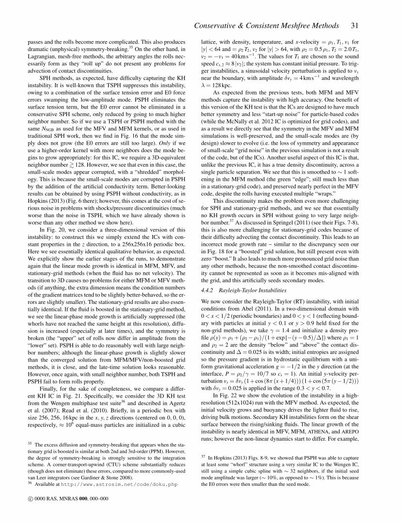


![A self-gravitating disc around L1527 IRS?arXiv:1304.7390v1 [astro-ph.SR] 27 Apr 2013 Mon. Not. R. Astron. Soc. 000, 000–000 (0000) Printed 27 July 2018 (MN LATEX style file v2.2)](https://static.documents.pub/doc/80x56/60ab8659447d0c69117d790e/a-self-gravitating-disc-around-l1527-irs-arxiv13047390v1-astro-phsr-27-apr.jpg)


![1 arXiv:1609.01283v2 [astro-ph.SR] 14 May 2017 · 2017. 5. 16. · Mon. Not. R. Astron. Soc. 000, 000{000 (0000) Printed 16 May 2017 (MN LATEX style le v2.2) The search for failed](https://static.documents.pub/doc/80x56/6142de917bbb8b33111717ff/1-arxiv160901283v2-astro-phsr-14-may-2017-2017-5-16-mon-not-r-astron.jpg)


