American Institute of Aeronautics and Astronautics

1

A New Flight Test Technique for Pilot Model Identification

Oliver Brieger1 and Daniel Ossmann2

DLR - German Aerospace Center, Institute of Flight Systems, 85077 Manching, Germany

Markus Rüdinger3

WTD 61 - German Bundeswehr Technical and Airworthiness Center for Aircraft, 85077 Manching, Germany

Matthias Heller4

EADS Military Air Systems, 85077 Manching, Germany

For today’s highly augmented fighter aircraft, the aircraft dynamics are specifically tai-

lored to provide Level 1 handling qualities over a wide regime of the service flight envelope.

This requires a profound understanding of the human pilot to assure that stability margins

of the airframe plus controller dynamics are sufficient to accommodate the additional pilot

dynamics introduced into the system during closed loop tasks. Whereas the mathematical

formulations of the airframe and controller dynamics are reasonably exact, the human pilot

remains to be the most unpredictable element in the Pilot Vehicle System. In the past dec-

ades various pilot models have been developed in conjunction with analytical handling quali-

ties and Pilot Involved Oscillations prediction criteria, mainly focusing on air-to-air tracking

tasks. This paper focuses on the development of a novel flight test technique, which allows

the identification of the pilot dynamics during air-to-surface aiming tasks. During an exten-

sive flight test campaign, data was gathered and processed, using state of the art system-

identification techniques to derive a mathematical model of the human pilot during air-to-

surface tracking tasks. Flight test and model-based data are compared with each other to

support the validity of the developed pilot models.

Nomenclature

AGL = Above Ground Level

AIM = Air Interceptor Missile

ATL = Above Target Level

ATLAS = Adaptable Target Lighting Array System

CFD = Chaff flare dispenser

DLR = Deutsches Zentrum für Luft- und Raumfahrt (German Aerospace Center)

DSFC = Direct Side Force Control

DTMF = Dual Tone Multi Frequency

EADS = European Aeronautic Defence and Space Company

FCS = Flight Control System

FOV = Field of View

GAF = German Air Force

GRATE = Ground Attack Test Equipment

HQR = Handling Qualities Rating (in accordance with Cooper-Harper rating scale)

HUD = Head-Up Display

IDS = Interdiction Strike

KIAS = Knots Indicated Airspeed

KTAS = Knots True Airspeed

1Group Leader, Flight Test Branch, Ingolstadt/Manching Airbase, Member. 2Research Scientist, Flight Test Branch, Ingolstadt/Manching Airbase, Member. 3Test Pilot, German Air Force, Aircraft Evaluation Division, Ingolstadt/Manching Airbase. 4Expert Advisor Flight Dynamics, Flight Dynamics, PO Box 80 12 29.

American Institute of Aeronautics and Astronautics

2

OTC = Official Test Center

PIO = Pilot-in-the-Loop-Oscillations

PVS = Pilot-Vehicle-System

TSPJ = Tip Stub Pylon Jammer

WTD 61 = Bundeswehr Technical and Airworthiness Center for Aircraft

C = Factor of the power spectrum of a multi step function

ci(x) = Distance between the aircraft and a single target

dx3y, dx3xi = Distances between the reference target x3/y3 and the targets xi resp. yi F = Transfer function

Fstx, Fsty = Stick transfer function

FP = Pedal transfer function

hst/hmin = Starting/minimum altitude of the test profile

Kg, Kr = Pilot gains

s(x) = Slant range/ test leg

sf = Minimum slant range at pull-up point

sSL = Projected slant range

sst = Initial slant range

td = Total tracking time

P = Piercing point coordinates between the line of sight and the target area plane

pcom = Pitch rate command

qcom = Roll rate command

xi,/yi = Longitudinal/Lateral targets

xSL, ySL = Slant range in the target area coordinate system

xAC,yAC,zAC= Aircraft coordinates in the target area coordinate system

xst ,xe = Start and end point of the test leg projection on the ground

xRT, yRT = Distances between P and the reference target x3/y3

xgr = Ground track of the (idealized) test leg

α* = Complementary angle

αi, βi = Aperture angles

βcom = Beta command

δx, δy/δp = Stick/Pedal Inputs

eΘ/eΨ = Pitch/heading error to the reference target

eΘ∗/eΨ

∗ = Pitch/heading error to the current active target

γ = Flight path angle

Θreq, Ψreq = Required pitch angle and heading tracking target

λ = HUD depression angle

ΨTA = Geographical orientation of the target area

I. Introduction

HE first concepts of modeling the human pilot by means of gathered empirical data have been generated during

World War II. After the first elementary applications in the years after the war, the development and utilization

of pilot models has increased tremendously with the rapid development of complex flight control systems. Most pi-

lot models are limited to one specific closed-loop task, as it is nearly impossible to derive a global mathematical de-

scription for the inherently nonlinear transitions in pilot behavior. Due to the unique human ability to learn, to adapt

to varying circumstances very quickly using a great variety of human sensors and to establish a wide range of Pilot

Vehicle System (PVS) organizations, the pilot is ‘modifier’ as well as ‘operating entity' within the system. Even for

one specific task (e.g. air-to-air refueling) the gross number of available sensing mechanisms to perceive and ana-

lyze perturbations in the environment and the strong influence of psychological factors such as stress, motivation or

even fear in emergency situations have great impact on human behavioral patterns. Another factor is the individual

mental constitution, which may affect pilot actions in various ways. All these characteristics make it extremely diffi-

cult to develop an appropriate mathematical model of the pilot, suitable for the assessment of handling qualities.

Nevertheless, numerous mathematical descriptions of man-machine-interaction have been derived in the past

decades and constitute the basis for a large number of handling qualities criteria, which are essential for the evalua-

tion of modern, highly augmented aircraft. For the description of the overall PVS the application of modern control

theory is appropriate. As shown in the example given in Fig.1 the pilot generates the necessary command action to

T T

American Institute of Aeronautics and Astronautics

3

minimize the system error between the actual and desired

aircraft pitch attitude Θ by processing the perceived infor-mation.

Early approaches are based on more or less complex

analytical descriptions of the pilot by using transfer and

describing function techniques to model the human pilot as

an active, dynamic control element. In the course of model

development, the pilot block in Fig. 1 has been enhanced

to include multiple, complex blocks, comprising sensor

channels, higher brain structures, the neuromuscular sys-

tem and biomechanics. Every one of these blocks proc-

esses and advances signal information and can be translated into a transfer/describing function. In other words, the

pilot model has grown from a very simple transfer element to a more complex structural model, with numerous feed-

back loops.

The assumption that the human operator can be described by a controller which estimates the state of the con-

trolled system and develops a control strategy to attain a defined performance index has led to the development of

the optimal control model, using optimal control theory. These models are rather complicated, but are capable of de-

scribing the human behavior in many different situations. Other fields of research focus on biomechanical descrip-

tions of the human pilot, analyzing acceleration influences on the pilot’s arm as a passive, biodynamic element

which may unintentionally induce control inputs. Such investigations are important to validate highly augmented

aircraft with respect to their sensitivity to acceleration coupling effects like role ratcheting.1 Today, engineers at-

tempt to model the human operator’s behavior using novel concepts based on fuzzy logic, neuronal networks or

Petri nets.1 These go as far as replicating the human decision making and learning process. All these approaches

have their legitimacy. Nevertheless, many state of the art handling qualities criteria, employed in the control law de-

sign process of modern fighter aircraft, make use of classical pilot models, based on linear/quasi-linear transfer func-

tions optimized for one specific closed-loop task. The vast majority of these models, mostly derived from flight test

data, have been developed for air-to-air tracking tasks. The work described herein, however, focuses on the identifi-

cation of a linear, structural pilot model, applicable to air-to-surface gun attacks. In order to achieve this aim, al-

ready existing structural models are used and adapted to the air-to-surface tracking task by means of system identifi-

cation. The main difference in terms of pilot behavioral patterns is that during air-to-air tracking a combination of

previewing and compensatory behavior can be observed. This is related to the significant lead compensation the pi-

lot can introduce into the closed-loop system when initially acquiring the target, anticipating the projected target tra-

jectory before transitioning to predominantly compensatory behavior during fine tracking. For the air-to-surface

tracking task described herein, the previewing element is minimized, requiring the pilot to employ a purely compen-

satory control strategy.

The associated flight tests have made extensive use of the newly developed Ground Attack Test Equipment II

(GRATE II), which is based on a ground deployed variable target system GRATE jointly developed by the German

Aerospace Center (DLR) and the Bundeswehr Technical and Airworthiness Center for Aircraft (WTD 61) in the

1980s, originally designed to assess the handling qualities of various combat aircraft during gun strafing.4 Since fu-

selage pointing is an extremely demanding task, requiring precise aircraft control, a method was sought which facili-

tates safe, repeatable, precise, high gain tasks during simulated ground attacks in a realistic, operationally relevant

environment. The system employs an array of lighted targets which are placed at specified positions on the ground.

During a prolonged dive attack the target lights are illuminated in a predefined sequence. The pilot’s task consists of

expeditiously acquiring and precisely tracking the respective lighted target, which appear to be selected randomly,

with an aircraft fixed reference until the next target is illuminated. The objective is to force the pilot to react con-

tinuously utilizing a high gain compensatory piloting technique, while minimizing any lead compensation. Conse-

quently, the closed-loop PVS is excited over a wide frequency range. This method was applied with great success in

1984 during the Direct Side Force Control (DSFC)-Alpha-Jet Program and proved to be very effective and reliable

in detecting handling qualities deficiencies. In 1987 NASA’s Dryden Flight Research Center developed a functional

equivalent of the system known as Adaptable Target Lighting Array System (ATLAS).6 Apart from the evaluation

of handling qualities this system is also suitable to investigate pilot dynamics, since it provides a precisely defined

input signal into the PVS. Provided that the mathematical descriptions of the airframe and controller dynamics are

accurate, the derivation of a suitable pilot model becomes viable. This second application of the GRATE-System has

been considered in the past but never realized. Unfortunately, both the original GRATE and ATLAS-Systems have

been lost over the past years, so that the development of a new, more sophisticated GRATE II-System became inevi-

table. A detailed system description is given in the following section. The determination of the target array geome-

Figure 1. Man-machine-control-loop (closed-

loop pitch tracking model)

Aircraft

disturbances

Θcom visual/displayed

perception Pilot

Θ ∆Θ δ

American Institute of Aeronautics and Astronautics

4

try, the target sequencing, defining the exciting function of the PVS, and the aircraft trajectory are of utmost impor-

tance. They define the quality of the gathered data and consequently the validity of the derived pilot model. A com-

prehensive description of the target sequences with respect to an optimized spectral density over a wide frequency

range and a detailed description of the flown attack profiles are given. To account for varying pilot perception and

technique three test pilots were involved in the flight test campaign and a total of 50 test runs have been performed.

The paper concludes with a portrayal of the system identification method used to process the gathered flight test data

using DLR’s system identification tool FITLAB (see Ref. 9, 10) to derive decoupled, linear pilot models for the lon-

gitudinal and lateral-directional motions which replicate pilot behavior during air-to-surface tracking. Time histories

generated with model data are then compared with actual flight test data to evaluate model fidelity.

II. Flight Test Preparation

A. Description of the GRATE II System

The main objective during the development of GRATE II

was to design an effective system, which offers maximum

flexibility with respect to transportability, time-efficient assem-

bly and simple reconfiguration capability while still fulfilling

flight test relevant requirements, such as response characteris-

tics and good visibility throughout the simulated gun attacks.

The latter is achieved by using high intensity approach lights as

commonly used for runway approach lighting systems. These

can be precisely adjusted in elevation angle and azimuth, to fo-

cus the beams on the projected approach flight path. The recon-

figuration aspect has been realized by using wireless technol-

ogy, enabling a quick adaptation to varying flight test objec-

tives (longitudinal or lateral-directional handling qualities evaluations, system identification). Every target unit con-

sists of three approach lights, each mounted on a ground

spike with an independent power supply (Fig. 2).

To provide as much flexibility as possible the target

sequences are generated using a graphical user interface

based on Matlab®, installed on a laptop. To avoid inter-

ferences with other frequencies, which may disturb the

transmission from the laptop to the targets and disrupt

test runs, unique DTMF (Dual Tone Multi Frequency)-

frequencies are used to command the switching of re-

ceiver relays and lamps. The DTMF audio signals gen-

erated with Matlab® are sent to the radio transmitter via

the sound output of the laptop. The transmitter routes

the audio signal to the receivers of all target units. Since

every unit has been assigned an individual frequency,

only those lights of the associated unit are illuminated

as long as the signal is transmitted. Figure 3 illustrates

the basic flight test set-up.

The pilot flies a race track pattern around the target

area as depicted in Fig. 4. Once established on the final

inbound run-in leg to the target area the test sequence is

initiated on the pilot’s call. The pilot then acquires and

tracks the illuminated targets using an aircraft-fixed

reference. The target sequences have been designed to

either excite the longitudinal motion, the lateral-

directional motion, or a combination of all three axes.

B. Definition of the Target Area Geometry and An-

gular Relationships

As described earlier, a fundamental prerequisite for the

accuracy of the subsequent pilot model identification

Radio

Figure 3. Flight test set-up

Target area

Ground Station:

radio, sequence generation,

transmitter,

Receiver +

Lamp

Aircraft

Figure 2. GRATE II target unit

Tracking-Point -

Roll-In

Pull-up Point

Base Distance

3.74 NM

Base Parameters

(400 kt/ 3664 ft )

3 NM

Figure 4. Target pattern

American Institute of Aeronautics and Astronautics

5

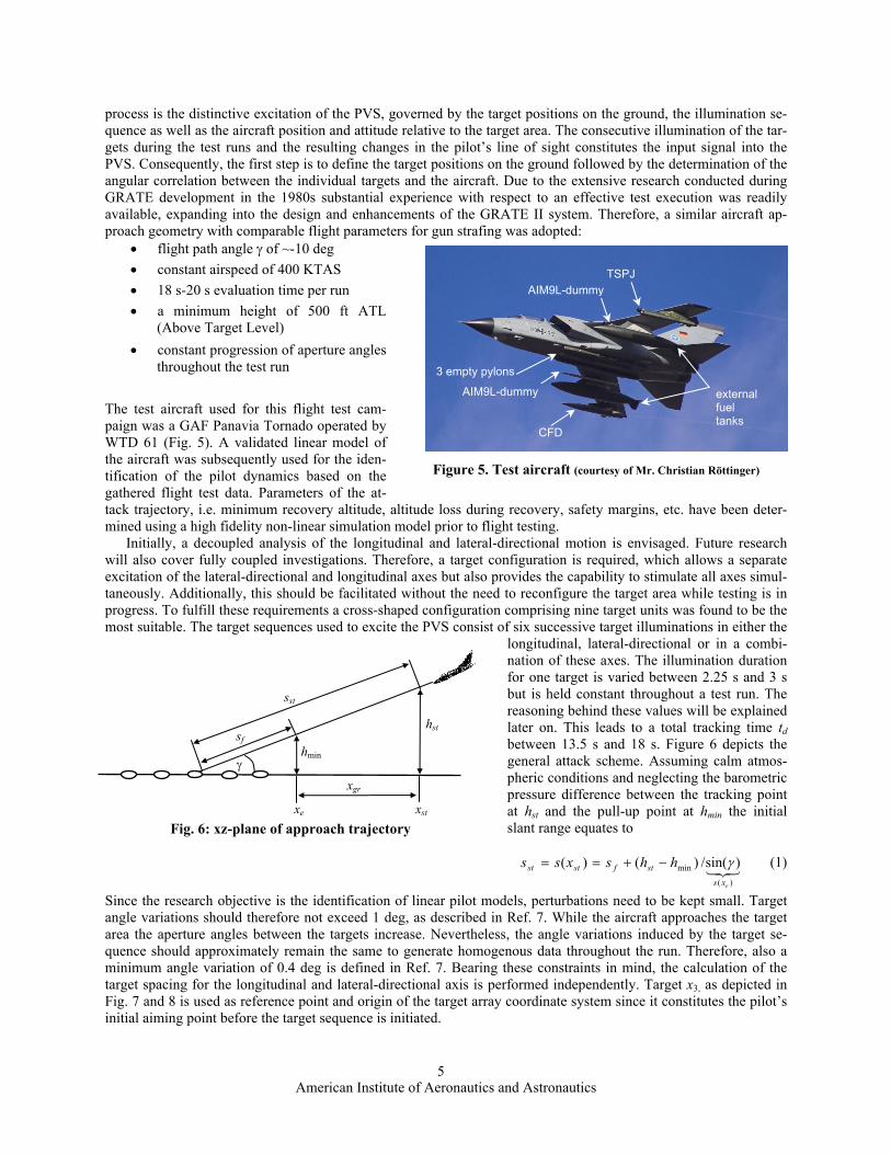
xgr

γ

xe xst

hmin

hst sf

Fig. 6: xz-plane of approach trajectory

sst

process is the distinctive excitation of the PVS, governed by the target positions on the ground, the illumination se-

quence as well as the aircraft position and attitude relative to the target area. The consecutive illumination of the tar-

gets during the test runs and the resulting changes in the pilot’s line of sight constitutes the input signal into the

PVS. Consequently, the first step is to define the target positions on the ground followed by the determination of the

angular correlation between the individual targets and the aircraft. Due to the extensive research conducted during

GRATE development in the 1980s substantial experience with respect to an effective test execution was readily

available, expanding into the design and enhancements of the GRATE II system. Therefore, a similar aircraft ap-

proach geometry with comparable flight parameters for gun strafing was adopted:

• flight path angle γ of ~-10 deg • constant airspeed of 400 KTAS

• 18 s-20 s evaluation time per run

• a minimum height of 500 ft ATL

(Above Target Level)

• constant progression of aperture angles

throughout the test run

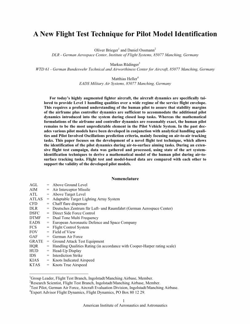
The test aircraft used for this flight test cam-

paign was a GAF Panavia Tornado operated by

WTD 61 (Fig. 5). A validated linear model of

the aircraft was subsequently used for the iden-

tification of the pilot dynamics based on the

gathered flight test data. Parameters of the at-

tack trajectory, i.e. minimum recovery altitude, altitude loss during recovery, safety margins, etc. have been deter-

mined using a high fidelity non-linear simulation model prior to flight testing.

Initially, a decoupled analysis of the longitudinal and lateral-directional motion is envisaged. Future research

will also cover fully coupled investigations. Therefore, a target configuration is required, which allows a separate

excitation of the lateral-directional and longitudinal axes but also provides the capability to stimulate all axes simul-

taneously. Additionally, this should be facilitated without the need to reconfigure the target area while testing is in

progress. To fulfill these requirements a cross-shaped configuration comprising nine target units was found to be the

most suitable. The target sequences used to excite the PVS consist of six successive target illuminations in either the

longitudinal, lateral-directional or in a combi-

nation of these axes. The illumination duration

for one target is varied between 2.25 s and 3 s

but is held constant throughout a test run. The

reasoning behind these values will be explained

later on. This leads to a total tracking time td

between 13.5 s and 18 s. Figure 6 depicts the

general attack scheme. Assuming calm atmos-

pheric conditions and neglecting the barometric

pressure difference between the tracking point

at hst and the pull-up point at hmin the initial

slant range equates to

321)(

min )sin(/)()(

exs

stfstst hhsxss γ−+== (1)

Since the research objective is the identification of linear pilot models, perturbations need to be kept small. Target

angle variations should therefore not exceed 1 deg, as described in Ref. 7. While the aircraft approaches the target

area the aperture angles between the targets increase. Nevertheless, the angle variations induced by the target se-

quence should approximately remain the same to generate homogenous data throughout the run. Therefore, also a

minimum angle variation of 0.4 deg is defined in Ref. 7. Bearing these constraints in mind, the calculation of the

target spacing for the longitudinal and lateral-directional axis is performed independently. Target x3, as depicted in

Fig. 7 and 8 is used as reference point and origin of the target array coordinate system since it constitutes the pilot’s

initial aiming point before the target sequence is initiated.

Figure 5. Test aircraft (courtesy of Mr. Christian Röttinger)

external fuel tanks

TSPJ

CFD

AIM9L-dummy

AIM9L-dummy

3 empty pylons

American Institute of Aeronautics and Astronautics

6

Figure 7 and 8 also show the target configuration for the excitation of the longitudinal axis. The aperture angles α1-

α4 between adjacent targets increase as the aircraft approaches. As depicted in Fig. 7 an equidistant spacing between

the target units would lead to α4 > α3 > α2 > α1 along the entire test section. While initially the angle variations

would be rather small, they would significantly increase as the aircraft progresses along the test leg. This effect

needs to be attenuated and a nearly uniform progression of the aperture angles α1-α4 has to be assured. Conse-

quently, the spacing between the target units has to be defined in such a way, that α3 equals 1 deg at the minimum

slant range s(xe) to meet the defined requirements stated above. This, however, leads to an α4(xe) greater than 1 deg. But since the last target change is triggered earlier at s(xe-∆x), where α4 is still within limits, this is considered ac-

ceptable. By observing these constraints the distance dx3x4 between the reference target x3 and target x4 can be deter-

mined by applying the sinus theorem, based on the geometric interrelationships described in Fig. 9.

)sin(

)sin()(

*

3

43 α

αxsd xx = (2)

By inserting the corresponding values at the pull-up point xe on the attack trajectory into Eq. (2) the distance dx3x4

can be calculated as follows:

m1225deg,10||deg,1)(with

)))(|(|sin(

))(sin(

))(sin(

))(sin()(

3

3

3

*

3

43

===

+−==

fe

e

e

fxx

sx

x

xs

x

xxsd

γα

αγπα

α

α (3)

This gives a distance dx3x4 of 112 m. Subsequently, the variation of α3 as a function of the aircraft ground track x can

be determined by applying the laws of sine and cosine:

= )sin(

)(arcsin)(

4

433 γα

xs

dx

x

xx (4)

with )cos()(2)()( 43

22

434 γxsdxsdxs xxxxx −+= (5)

The remaining aperture angles α4, α2 and α1 can then be expressed accordingly:

hmin

γ

dx1x3 c1(s)

α1+α2

s(x)

x1 x2 x3 x4 x5 xe test ground dist. xst

sf

Figure 7. Angular relationships Figure 8. Characteristic distances

xgr ∆x

α4

α1

x

α1-α4

α2 α3

xe xst

x1 x2 x3 x4 x5

x2 x3 x4

dx3x4

s(x3)=s(x)

γ

α3

c4(x)

α* dx3x2

π−γ

α2

Figure 9. Slant range geometry

American Institute of Aeronautics and Astronautics

7

s(x)

β1

β3

β4

β2

2dx3y

y1

y2

y3 = x3

y4

y5

xgr xe xst

x

Figure 11. xy-plane of the approach trajectory

y

y

)()sin()(

arcsin)( 3

5

534 s

xs

dx

x

xx αγα −

= (6)

with )cos()(2)()( 53

22

535 γxsdxsdxs xxxxx −+= (7)

−= )sin(

)(arcsin)(

2

232 γπα

xs

dx

x

xx (8)

with )cos()(2)()( 23

22

232 γπ −−+= xsdxsdxs xxxxx (9)

)()sin()(

arcsin)( 2

1

13

1 xxs

dx

x

xx αγπα −

−= (10)

with )cos()(2)()( 13

22

131 γπ −−+= xsdxsdxs xxxxx (11)

The distances between the remaining targets and the reference target x3, dx3x5, dx3x2, and dx3x1 are determined by

means of a numerical optimization method to obtain an approximately homogenous progression of the aperture

angles as a function of the covered ground distance. This is to ensure comparable angle alterations throughout the

test run. The employed algorithm minimizes the error between the enclosed reference area defined by the integral of

Eq. (4) and the integrals of Eq. (6), (8) and (10) as described in Eq. (12):

4,2,1),()()(33 3 =−= ∫∫ mdxdxdxxde

e

st

m

e

st

m

x

x

xxm

x

x

xx αα (12)

The resulting distances are listed in Tab. 1 below.

dx3x1 258 m

dx3x2 123 m

dx3x4 112 m

dx3x5 214 m

Table 1. Distances between the reference target x3 and xi

Figure 10 depicts the aperture angle progression of α1-α4

as a function of the covered ground distance x. It is evident

that initially the angle values are relatively small, around 0.2

deg. To warrant angle alterations between 0.4 deg and 1 deg,

initially only every other target is illuminated while towards

the end of the run adjacent targets are activated. An ex-

emplary sequence for the longitudinal axis is x1 → x4 →

x2 → x4 → x3 → x2 (please refer to Fig. 7).

To finalize the definition of the target cross

configuration the distances between the targets for the

excitation of the lateral-directional motion (excitation

along the y-axis of the target array) as illustrated in Fig.

11 have to be determined. These are spaced with

identical increments due to symmetry aspects. Since

again the small purtubation approach applies, the

following assumption can be made: tan(β) = β for β << π. With the requirement β (xe) = 1 deg the lateral distances between target units can then be calculated,

which in turn enables the determination of the

α1

α2

α3 α4

Visual Angle [deg]

Distance x to reference target [m]

xst xe

Distance x to the reference target [m]

Aperture angles [deg]

Figure 10. Aperture angle progression as a

function of covered ground distance

American Institute of Aeronautics and Astronautics

8

progression of the angles β1-β4 along the test leg s(x). By solving Eq. (14) the equidistant lateral spacing dx3y equates to

21.5 m.

=

)(arctan)(

3

xs

ds

yx

iβ (13)

with )180/sin()180/sin(

)(3 π

πγπ −−±=

xsd yx (14)

An excitation sequence for the lateral-directional axes is

for example is y3 → y6 → y4 → y3 → y7 → y5 (please refer to

Fig. 11).

The target array layout has now been defined. Albeit a

fully coupled investigation has not yet been conducted for the

initial pilot model identification process, which focuses on

the development of decoupled longitudinal and lateral-

directional models, the resulting angular relationships for an

excitation of the PVS in multiple axes can be determined as

follows. The cross array allows numerous angle variations by

alternately illuminating targets in the x- and y-axis as

depicted in Fig. 12, showing all but the mirror-symmterical

target combinations. In the following, the derivation for one

exemplary set of angles will be presented, the remaining sets

are obtained accordingly. An illustration of the angular

relationships for the calculation of δx1y1(x), the enclosed angle between target unit x1 and y1 is depicted in Fig. 13. The slant

range sy1(x) between the aircraft and target unit y1 can be

determined with the given distance dx3y (Eq. (14)). The slant

range s(x) = sx3(x) = sy3(x) to the reference target in the origin

of the target array is calculated by:

2

3

2

1 4)()( yyy dxsxs += (15)

For the determination of the angle δx1y1(x) the ground distance dx1y1 is required. This is easily derived by:

2

13

2

311 4 xyyxyx ddd += (16)

Finally, the angle δx1y1(x) can be expressed by applying the law of cosines and substituting Eq. (11), (15) and (16):

)()(2

)()(arccos)(

11

2

21

2

1

2

1

11xsxs

dxsxsx

xy

xxxy

yx

−+=δ (17)

The remaining angles δxiyi(x) are calculated accordingly, by inserting the slant ranges sxi(x) and syi(x) for i=1:9. The

postulated limits between 0.4 deg and 1 deg are also valid for the combined excitations. In Fig. 14 the resulting

angle progressions, with the color code used to highlight target changes in Fig. 12, are plotted as a function of

covered ground distance. It shows the defined angular limits of 0.4 deg and 1 deg and the position of the last

possible target alteration. This is defined by the transition from the 5th to the 6th target prior to pull-up and the

longest illumination interval of 3 s. Fig. 14 therefore defines the possible target combinations within the given

limits. To warrant angle alterations between 0.4 deg and 1 deg, initially the consecutive illumination of the outer

targets in both axes is favorable (target alterations defined by the red and black curves) while towards the end of the

run the inner targets have to be activated (target alterations defined by the blue curves); also refer to Fig. 12 for

conclusiveness.

x3

sx1(x)

2dy3y

sy1(x)

x1

y1

dx3x1

β1+β2

α1+α2

s(x)

δy1x1=?

dx1y1

Figure 13. Angular relationships for δδδδx1y1(x)

x1

x2

y1 y2 x3=y3

x4

y5

x5

y

x

21.5 m

256 m

Figure 12. Possible target combinations for com-

bined inputs

43 m

43 m 21.5 m

214 m

123 m

112 m

y4

Distance x to Reference Target [m]

1°-limit

Latest

angle jump 0.4°-limit V

isual Angle [deg]

Figure 14. Progression of combined aperture angles

range

xst

Latest angle

alteration

xe

Aperture angles [deg]

Distance x to the reference target [m]

American Institute of Aeronautics and Astronautics

9

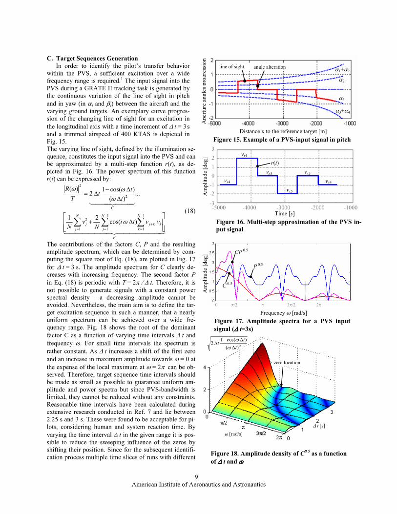
C. Target Sequences Generation

In order to identify the pilot’s transfer behavior

within the PVS, a sufficient excitation over a wide

frequency range is required.1 The input signal into the

PVS during a GRATE II tracking task is generated by

the continuous variation of the line of sight in pitch

and in yaw (in αi and βi) between the aircraft and the varying ground targets. An exemplary curve progres-

sion of the changing line of sight for an excitation in

the longitudinal axis with a time increment of ∆ t = 3 s and a trimmed airspeed of 400 KTAS is depicted in

Fig. 15.

The varying line of sight, defined by the illumination se-

quence, constitutes the input signal into the PVS and can

be approximated by a multi-step function r(t), as de-

picted in Fig. 16. The power spectrum of this function

r(t) can be expressed by:

4444444 34444444 21

444 3444 21

P

N

k

kkj

N

j

N

j

j

C

vvtiN

vN

t

tt

T

R

∆+

∆

∆−∆=

∑∑∑−

=+

−

==

1

1

1

11

2

2

2

)cos(21

...)(

)cos(12

)(

ω

ωωω

(18)

The contributions of the factors C, P and the resulting

amplitude spectrum, which can be determined by com-

puting the square root of Eq. (18), are plotted in Fig. 17

for ∆ t = 3 s. The amplitude spectrum for C clearly de-

creases with increasing frequency. The second factor P

in Eq. (18) is periodic with T = 2π / ∆ t. Therefore, it is not possible to generate signals with a constant power

spectral density - a decreasing amplitude cannot be

avoided. Nevertheless, the main aim is to define the tar-

get excitation sequence in such a manner, that a nearly

uniform spectrum can be achieved over a wide fre-

quency range. Fig. 18 shows the root of the dominant

factor C as a function of varying time intervals ∆ t and frequency ω. For small time intervals the spectrum is

rather constant. As ∆ t increases a shift of the first zero and an increase in maximum amplitude towards ω = 0 at the expense of the local maximum at ω = 2π can be ob-served. Therefore, target sequence time intervals should

be made as small as possible to guarantee uniform am-

plitude and power spectra but since PVS-bandwidth is

limited, they cannot be reduced without any constraints.

Reasonable time intervals have been calculated during

extensive research conducted in Ref. 7 and lie between

2.25 s and 3 s. These were found to be acceptable for pi-

lots, considering human and system reaction time. By

varying the time interval ∆ t in the given range it is pos-sible to reduce the sweeping influence of the zeros by

shifting their position. Since for the subsequent identifi-

cation process multiple time slices of runs with different

∆ t [s]

ω [rad/s]

2)(

)cos(12

t

tt

∆

∆−∆

ωω

zero location

Figure 18. Amplitude density of C0.5 as a function

of ∆∆∆∆ t and ωωωω

line of sight angle alteration

α3+α4

α3

α2

α1+α2

Figure 15. Example of a PVS-input signal in pitch

Distance x to the reference target [m]

Aperture angles progression

Figure 17. Amplitude spectra for a PVS input

signal (∆∆∆∆ t=3s)

Frequency ω [rad/s]

CP 0.5

C 0.5

P 0.5

0 π/2 π 3π/2 2π

Amplitude [deg]

Figure 16. Multi-step approximation of the PVS in-

put signal

Amplitude [deg]

-5000 -4000 -3000 -2000 -1000

r(t)

vx1

vx5

vx3

vx4 vx4

vx3

Time [s]

3

2

1

0

-1

-2

-3

American Institute of Aeronautics and Astronautics

10

target time intervals are used, the resulting model is valid for a broad frequency range without encountering short-

comings in signal quality evoked by zeros in the amplitude spectrum. In summary, the PVS-input signals for the ex-

citation of individual and multiple axes are obtained by means of a complex optimization algorithm which considers

the following constraints:

• Variation of ∆ t between 2.25 s and 3 s (0.15 s increments)

• Uniform amplitude spectrum

• Angle alterations limited to 0.4 - 1.0 deg

• Longitudinal transitions to the final 6th target are always ‘nose up’ for flight safety reasons

D. Determination of System Inherent Time Delays

An extensive study regarding system inherent time lags has been conducted, to determine rise and decay times of

the 200 Watt approach lights, since this significantly affects pilot reaction time. Specifically the period of time from

the instant the DTMF-signal is transmitted to the respective target unit until the light intensity has reached a level

that the pilot becomes aware of the target change, is essential. Equally important is the determination of the decay

time, since the decay of the light intensity of the high intensity lights is much slower than the onset, which can lead

to a delayed shift of attention, because the pilot may still focus on the deactivated target, while the new target is al-

ready visible. A complex test setup was devised to measure the target lamp performance and to derive a mathemati-

cal approximation. The setup included an infra-red LED to measure light intensity and measurement devices, re-

cording signal generation, signal transmission and relay switching. The decay behavior is approximated by a 7th-

order polynomial, while the onset behavior is approximated by multiple functions, including linear and 5th-order ap-

proximations, as depicted in Fig. 19.

Since the activation of the new target and the deactivation of the old target occur simultaneously, it is difficult to

determine, to which stimulus the pilot will react to. For the determination of the inherent system time delay the

worst case is assumed, where the pilot may continue to track the already deactivated target, due to the much slower

decay in light intensity, before becoming aware that a new target has been activated. Earlier flight tests using

GRATE II have shown that an average 0.5 sec system inherent time delay is a good first estimate and may be

changed as a result of the system identification process.

III. Flight Test Execution

A. Test Aircraft

The test bed for this test was a GAF Tornado PA200 Interdiction Strike (IDS) Version with variable wing sweep

geometry. The external aircraft configuration consisted of two external 1500 ltrs fuel tanks on the inboard wing sta-

tions, a chaff/flare dispenser (CFD) and a jamming pod (TSPJ) on each outboard wing station. Additionally, two Air

Interceptor Missiles (AIM-9L) dummies were carried on both side wall stations (see Fig.5). This test configuration

is a standard aircraft configuration, as well as mission representative (typical egress phase during a combat sortie

with all bombs delivered). Total aircraft weight varied between approximately 47.000 lbs on the first run to 31.000

lbs on the last run.

For post flight data analysis the onboard test recording equipment was used as well as the standard video system,

which recorded the HUD-video and the right multi-function display in the rear cockpit. The sample rate for all flight

relevant parameters ranged from 8 Hz-16 Hz. From the three possible wing sweep settings (25 deg, 45 deg and 67

Light Intensity [%]

Figure 19. Mesured and approximated onset and decay beavior

Time [s] Time [s]

a) Onset behavior: b) Decay behavior:

measured

approximated

measured

approximated

American Institute of Aeronautics and Astronautics

11

deg) the 45 deg setting was used for all test runs, since this is the most likely configuration in the low altitude re-

gime. Furthermore, the manual selectable slats were set to ‘in’.

The flight control system of the aircraft is a complete irreversible fly-by-wire system, with pitch-/ roll-rate and

sideslip angle command. Pitch is controlled via the symmetric deflection of the all movable taileron, whereas roll-

control is achieved by the asymmetric deflections of the taileron surfaces assisted by one pair of spoilers on each

wing. Yaw is commanded via a classical rudder.

B. Test Pattern Description

In order to maximize the possible test-runs per sortie a typical race track pattern as depicted in Fig. 4, was estab-

lished known from typical air-to-ground bombing ranges. All legs of the pattern were planned as to arrive on the fi-

nal run-in with the correct flight parameters considering aircraft weight and configuration. Based on the chosen

flight path angle, the required evaluation time and the planned airspeed on the final test-leg, the entire geometry and

the respective altitudes were calculated backwards. Different roll-in techniques were taken into account as well as

approximately 2.3 s to establish and stabilize the parameters after rolling out on final. Furthermore, a minimum alti-

tude over the test area was set to 500 ft AGL and an altitude loss during dive recovery of 250 ft (4 g recovery) con-

sidered.

C. Run-In Parameters

The flight-test parameters on the

evaluation leg of the pattern were chosen

based on operational relevance for typical

air-to-ground tasks while still fulfilling all

test requirements. The flight path angle

was therefore set to -10 deg, which is gen-

erally the minimum angle for a typical air-

to-ground gun attack. A steeper approach

would have been more advantageous in a

tactical environment; however, this would

have required a longer final run-in leg due

to the higher recovery altitude after the

dive, possibly impairing the visibility of

the target lights under all lighting condi-

tions. Target airspeed was governed by the same trade-off between operational and test requirements and was set to

400 KTAS, which was equal to approximately 385 KIAS considering the atmospheric conditions during the tests. In

Fig. 20 a cross section of the final run-in with all relevant descriptions is depicted.

D. Piloting Requirements

All aircrew were test-crews from the German Official Test Center (OTC) at Manching (qualified test pilots with

at least 1400 flying hours) and rated on this aircraft type. A total of three flights with three different pilots were con-

ducted. Each sortie consisted of a familiarization phase and a dedicated test phase. The familiarization phase con-

sisted of two runs to become acquainted with the test pattern and equipment; these two runs were also used to con-

firm the pre-planned test pattern and optimize the alignment maneuver onto the final test leg. Afterwards 12-18

dedicated test-runs were conducted.

The combined task for the pilot during the evaluation consisted of an aggressive acquisition and precise tracking of

the respective illuminated target. As aiming device, the reversionary bombing sight, projected into the HUD-FOV

was used; this was calibrated once and not changed during all three test flights.

IV. System Identification and Pilot Model Development

A. System Identification

For the identification of a pilot model for air-to-surface tracking tasks, system identification software developed

at DLR Braunschweig called FITLAB is utilized.10 The basic concept of system identification is to derive a mathe-

matical description of a dynamic system from the observed (measured) response z to a known input u, by determin-

ing the underlying parameters p which govern system behavior (see Fig. 21). For the objective described herein two

steps need to be performed: First, the correct model structure (system state function f and observation function g) de-

scribing the transfer behavior between u and z needs to be defined. Secondly, the system parameters p have to be

Figure 20. Test profile

American Institute of Aeronautics and Astronautics

12

estimated by utilizing system identification methods which use

the measured input and output data. The identification of the

system parameters p in the time domain, as applied here, is

based on a maximum likelihood estimation employing numeri-

cal algorithms such as Gauss-Newton. A detailed description of

the theoretical background of system identification methods

would go beyond the scope of this paper, for a comprehensive,

detailed treatment please refer to Ref. 9. The described ap-

proach of model development and parameter estimation is an

iterative process, possibly requiring changes and adaptations

within the model structure to achieve better identification re-

results.

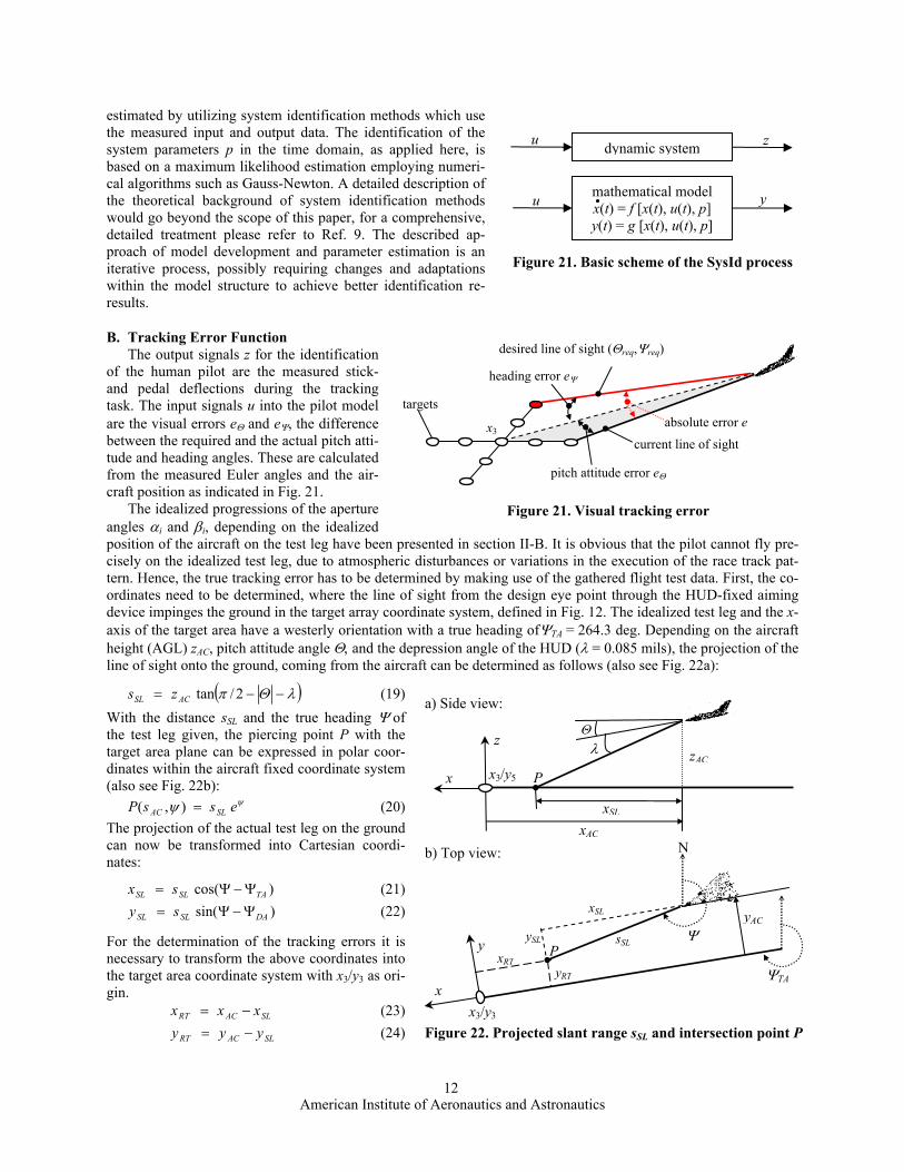
B. Tracking Error Function

The output signals z for the identification

of the human pilot are the measured stick-

and pedal deflections during the tracking

task. The input signals u into the pilot model

are the visual errors eΘ and eΨ, the difference

between the required and the actual pitch atti-

tude and heading angles. These are calculated

from the measured Euler angles and the air-

craft position as indicated in Fig. 21.

The idealized progressions of the aperture

angles αi and βi, depending on the idealized position of the aircraft on the test leg have been presented in section II-B. It is obvious that the pilot cannot fly pre-

cisely on the idealized test leg, due to atmospheric disturbances or variations in the execution of the race track pat-

tern. Hence, the true tracking error has to be determined by making use of the gathered flight test data. First, the co-

ordinates need to be determined, where the line of sight from the design eye point through the HUD-fixed aiming

device impinges the ground in the target array coordinate system, defined in Fig. 12. The idealized test leg and the x-

axis of the target area have a westerly orientation with a true heading ofΨTA = 264.3 deg. Depending on the aircraft

height (AGL) zAC, pitch attitude angle Θ, and the depression angle of the HUD (λ = 0.085 mils), the projection of the

line of sight onto the ground, coming from the aircraft can be determined as follows (also see Fig. 22a):

( )λΘπ −−= 2/tanACSL zs (19)

With the distance sSL and the true heading Ψ of the test leg given, the piercing point P with the

target area plane can be expressed in polar coor-

dinates within the aircraft fixed coordinate system

(also see Fig. 22b): ψψ essP SLAC =),( (20)

The projection of the actual test leg on the ground

can now be transformed into Cartesian coordi-

nates:

)cos( TASLSL sx Ψ−Ψ= (21)

)sin( DASLSL sy Ψ−Ψ= (22)

For the determination of the tracking errors it is

necessary to transform the above coordinates into

the target area coordinate system with x3/y3 as ori-

gin.

SLACRT xxx −= (23)

SLACRT yyy −= (24)

Θ λ

x3/y5

xSL

zAC

x3/y3

sSL Ψ

N

xSL

ySL y

x

x

z

xRT yRT

xAC

yAC

ΨTA

Figure 22. Projected slant range sSL and intersection point P

P

P

b) Top view:

a) Side view:

targets

current line of sight

pitch attitude error eΘ

heading error eΨ

desired line of sight (Θreq,Ψreq)

absolute error e

Figure 21. Visual tracking error

x3

dynamic system u z

mathematical model

x(t) = f [x(t), u(t), p]

y(t) = g [x(t), u(t), p]

u y

Figure 21. Basic scheme of the SysId process

American Institute of Aeronautics and Astronautics

13

Significant deviations from the planned attack heading of ΨTA = 264.3 deg would have the effect, that the target al-

terations in pitch would inevitably lead to undesired coupling between the longitudinal and lateral-directional axes.

As described in Ref. 8, the GRATE II flight tests have shown that deviations in heading angle do not exceed ±2 deg,

having, therefore, a negligible effect on the tracking error function. The longitudinal tracking error eΘ can then be

expressed as:

( )[ ]λπν +Θ−−=Θ 2/e (25)

with

=

+=

AC

AC

AC

RTSL

z

x

z

xsarctanarctanν (26)

The lateral tracking error is given by:

=

+=

AC

AC

RTSL

RT

x

y

xs

ye arctanarctanΨ (27)

So far, only the tracking errors with respect to

the reference target unit x3/y3 have been deter-

mined. The tracking error regarding the cur-

rently illuminated target unit can easily be cal-

culated by correcting, xRT and yRT with the given

distances dx3xi and dx3y (determined earlier in

section II-B).

In Fig. 24 time histories of the angular er-

rors eΘ and eΨ for a combined excitation se-

quence are shown. Clearly visible are the

changes in tracking error magnitude when

switching from one target to another every 3

sec. After each target alteration the pilots tries

to minimize the longitudinal and lateral track-

ing error.

C. System Identification

The analysis of the flight test data has shown that during a solely longitudinal or lateral-directional excitation of

the PVS the pilot focuses on the currently excited axis, neglecting any error in the other axes as long as it is small.

Hence, if a single-axis excitation is given, the identification process can be focused on this axis alone. An elemen-

tary block diagram is depicted in Fig. 25. The linear pilot model is developed in a step-by-step approach, starting

with the longitudinal axis, followed by the more complex lateral-directional axes. It is based on the crossover model

theory described in Ref. 2 and the structural model developed in Ref. 3.

Θ+λ

x3/y3

zAC

x3/y3

sSL = xSL

Ψ = ΨTA

y

x

x

z

xRT

yAC = yRT

xAC = sSL + xRT

ν eΘ

eΨ

Figure 23. Geometrical depiction of the angular errors

b) Lateral error eΨ:

a) Longitudinal error eΘ:

Figure 24. Example of eΘΘΘΘ and eΨΨΨΨ during a combined test run

target alteration Pitch Error e Θ [deg]

Heading Error e Ψ [deg]

Time [s] Time [s]

American Institute of Aeronautics and Astronautics

14

Longitudinal Axis

During an air-to-surface tracking task with an excitation of the longitudinal axis, the pilot attempts to minimize

the error eΘ. Hence, the pilot closes the loop for pitch attitude control Θ to determine the current error with respect to

the illuminated target unit. For highly augmented aircraft, the pilot’s stick input can be converted into various com-

mand signals, depending on the control law design. In the case of the Tornado the pilot commands the desired pitch

rate qcom by longitudinal stick deflections. Since the pilot uses the pitch attitude Θ to control the aircraft during the tracking task, the transfer behavior qcom → Θ is characterized by a single integral with a proportional element (K/s)

(see Ref. 2), when considering the short term dynamics only (which can be assumed for this application since target

sequencing is very quick). The derived pilot model is shown in Fig. 26.

The applicable state equation is easily derived and can be stated as follows: s

rpgpx eeKeK τδ )( ΘΘ += & (28)

The model takes the following aspects into account: the error signal eΘ is delayed by eτs (1st order Pade-

approximation), to account for the processing time required by the pilot to recognize target changes and generate

appropriate stick inputs δx. The total time delay is assumed to be 0.8 sec, 0.5 sec attributed to the GRATE II system

as described in section II-D and 0.3 sec of

pilot delay, as commonly used in many

handling qualities criteria. When acting on

the error signal the pilot uses two sources

of information; firstly, the absolute differ-

ence between desired and commanded

pitch attitude represented by the Kgp pro-

portional path, and secondly, the perceived

rate of change of the error, described by the

proportional and derivative path. Hence,

the K/s transfer behavior of the open loop

PVS described by the crossover model, as

proposed in Ref. 2, is confirmed, however

augmented with an additional rate com-

mand path.

Figure 27 shows the results of the sys-

tem identification process for the longitu-

dinal axis. An average time delay has been

Aircraft

dynamics β1-β4

Θ Pilot

dynamics

eΘ δx

Ψ

α1-α4

_

_

eΨ δP

δy

Figure 25. In- and outputs of the pilot, minimizing both errors by the use of all three

control devises

Θ Krp

eΘ εx _

Kgp

s

eτs aircraft

dynamics

Κ/s

Fstx qcom δx

Figure 26. Pilot model structure for the longitudinal axis

Pilot

Figure 27. Longitudinal pilot dynamics

Pitch Error e Θ [rad]

Stick Input δ x [rad]

Time [s]

measured

identified

τ

American Institute of Aeronautics and Astronautics

15

estimated, which correlates with the initial approximation quite accurately. Deviations in stick amplitude may be as-

sociated with non-linear pilot dynamics, non-linear elements in the flight control system, and shortcomings in the pi-

lot model, such as for instance neuro-muscular dynamics that have not been considered.

• Lateral-directional Axes

Contrary to the longitudinal excitation, the pilot controls two axes using rudder and aileron to minimize the error

eΨ during a pure lateral excitation. Similarly to the pitch axis, a (roll-) rate command system is used to control the

aircraft. In the directional axis sideslip angle β is directly controlled using the rudder, as a result inducing a change in heading angle Ψ. Flight test data analysis has shown that all pilots mainly used the rudder to place the aiming

sight on the target, supported by only small roll inputs. The reason is that the aircraft response is very precise when

mainly working with the pedals, combined roll-yaw inputs, when attempting to realign the aircraft on a straight tra-

jectory towards the target led to overshoots and a significantly higher workload. The pilot model for this case is

shown in Fig. 28.

The associated state equations are: s

rrgry eeKeK τδ )( ΨΨ += & (29)

s

rygyP eeKeK τδ )( ΨΨ += && (30)

Again, the elements FP and Fsty are in-

cluded to describe the roll stick and pedal

characteristics. The error eΨ is again fed

through a time delay eτs, before being ad-

vanced to the two paths, generating the inputs

for the rudder and the aileron. In analogy to

the longitudinal pilot model the roll axis is

again split into a proportional Kgr and a paral-

lel derivative path with an associated gain Krr

acting on the errors’ rate of change. Since the

Tornado’s numerator time constant TΦ2 is

rather high, leading to relatively slow flight

path dynamics, the transfer behavior pcom → Ψ can be described by a K/s-approximation.

Again, this leads to the K/s crossover behav-

ior, augmented with an additional derivative

element, describing the pilot’s efforts to con-

trol the rate of change of the error.

Ψ

Krr

eΨ

δy

εy _

Kgr

eτs aircraft

dynamics

Kgy s-1

δP

s

Κ/s

Κ

missing

integral

s

Fsty

Fp

pcom

βcom

Figure 28. pilot model structure for the lateral-directional axis

Kry

Pilot

measured

identified

Figure 29: System identification time histories

Heading Error

e Ψ [deg]

Stick Input

δ y [rad]

Paddles Input

δ P [mm]

Time [s]

measured

identified

American Institute of Aeronautics and Astronautics

16

The lower path generates the pilot’s rudder pedal inputs. The FCS features sideslip control (βcom), leading to a proportional correlation between the pedal input and the aircraft heading, since a change in sideslip angle directly

induces a heading change. In order to realize the crossover model transfer characteristics (K/s) described in Ref. 2,

an additional integration needs to be performed by the pilot, leading to the cancellation of the derivative in the rate

path (Kry) and the addition of an integral block in the proportional path (Kgy) as depicted in Fig. 28.

Figure 29 shows time histories of pilot inputs extracted from flight test data which are then compared to stick

and pedal signals generated with the identified linear pilot model. Again, variable time delays and amplitude varia-

tions can be observed. This highlights the difficulties in the attempt to replicate a highly nonlinear system such as

the human pilot by means of quasi-linear models, even for a very confined test setup with very small perturbations.

In the given example the pilot uses sideslip and roll to the same extent to control the aircraft, making a correct iden-

tification even more difficult, due to considerable coupling effects. For cases, where pure sideslip control was used

to minimize the lateral error eΨ significantly better system identification results could be achieved, which has been

verified in practice.

V. Conclusion

The work described herein is regarded as a first step on the way to a more sophisticated pilot model for air-to-

surface tracking. It was shown that the GRATE II system is an invaluable tool to investigate pilot dynamics in a re-

alistic, operationally relevant environment, which cannot be achieved to the same degree when employing HUD-

based generic tracking tasks. Further efforts will be made to refine the derived models to include combined, fully

coupled dynamics, switching functions to address varying pilot control strategies and biomechanical aspects to ac-

count for interactions between the airframe dynamics and the physical properties of the human extremities used to

manipulate the control devices.

Acknowledgment

The authors would like to thank the involved organisations for their extensive support. Without the close col-

laboration between the German Aerospace Center (DLR), the Bundeswehr Technical and Airworthiness Center for

Aircraft (WTD 61) and the European Aeronautic Defence and Space Company (EADS) this work would not have

been possible.

References 1 Höhne, G., “Roll Ratcheting: Cause and Analysis,” DLR-FB 2001-15,Braunschweig, 2001. 2 McRuer, D., “Mathematical Models of Human Pilot Behavior,”AGARD-AG-188, Neuillysur Seine, 1974. 3 Hess, R. A., “A Structural Model of the Adaptive Human Pilot,” AIAA Guidance, Navigation and Control Conference,

AIAA-87-2523. 4 Shafer, M.S., “Initial flight test of a ground deployed system for flying quality assessment,” NASA Technical Memoran-

dum 101700, Edwards, California, 1989. 5 Einsiedel, F., “GRATE II – Implementation of a ground deployed system for the evaluation of handling qualities,” IB 111-

2007/49, Braunschweig/ Manching, 2007. 6 Koehler, R., “GRATE – A new flight test tool for flying qualities evaluations,” 73rd Symposium on Flight Test Techniques,

AGARD, 1988. 7 Koehler, R., “Design and Implementation of Input Signals for Identification of Pilot/Aircraft Models,” DFVLR-FB 84-08,

Braunschweig, 1984. 8 Ossmann, D., “Identification of a pilot model on the basis of flight test data for handling quality evaluation,” Master Thesis,

Technische Universität München, Institute of Flight System Dynamics, Munich, 2008. 9 Jategaonkar, R. V., Flight Vehicle System Identification: A Time Domain Mythology, AIAA, Reston, Virginia, 2006. 10 Seher-Weiß, S., “User's Guide FITLAB Parameter Estimation Using MATLAB Version 2.0,” IB 111-2007/27, Braun-

schweig; 2007.