Feola et al. EURASIP Journal on Advances in Signal Processing (2015) 2015:28 DOI 10.1186/s13634-015-0207-0

RESEARCH Open Access

A new frequency approach for light flickerevaluation in electric power systemsLuigi Feola*, Roberto Langella and Alfredo Testa

Abstract

In this paper, a new analytical estimator for light flicker in frequency domain, which is able to take into account alsothe frequency components neglected by the classical methods proposed in literature, is proposed. The analyticalsolutions proposed apply for any generic stationary signal affected by interharmonic distortion. The light flickeranalytical estimator proposed is applied to numerous numerical case studies with the goal of showing i) thecorrectness and the improvements of the analytical approach proposed with respect to the other methodsproposed in literature and ii) the accuracy of the results compared to those obtained by means of the classicalInternational Electrotechnical Commission (IEC) flickermeter. The usefulness of the proposed analytical approach isthat it can be included in signal processing tools for interharmonic penetration studies for the integration ofrenewable energy sources in future smart grids.

Keywords: Light flicker; IEC flickermeter; Interharmonic; Distributed energy resources; Power quality; Smart grids

1 IntroductionLight flicker (LF) phenomenon is still considered one ofthe most important power quality (PQ) problems due toits ability to be directly perceived by customers, produ-cing complaints from them.LF is caused by the modulation of the supply funda-

mental voltage, which produces modulated light emis-sions whose severity, in terms of annoying effects onhumans, depends on modulation amplitudes and fre-quencies as well as on lamp technologies [1]. LF iscommonly measured by means of the InternationalElectrotechnical Commission (IEC) flickermeter [2]that, for historical reasons, was designed and testedonly with reference to voltage amplitude modulation(AM), which was the first source of LF identified and refer-ring only to 60-W incandescent bulbs, which were the mostdiffused lamps all over the word at that time.Today, incandescent lamps are going to be banned,

in particular in Europe, Australia and North America,but the IEC flickermeter is still the only instrumentused also because international standards are basedon it.

* Correspondence: luigi.feola@unina2.itDepartment of Industrial and Information Engineering, Second University ofNaples, DIII-SUN, Via Roma, 29, 81031 Aversa, Caserta, Italy

© 2015 Feola et al.; licensee Springer. This is anAttribution License (http://creativecommons.orin any medium, provided the original work is p

The main drawbacks of the IEC flickermeter are asfollows: i) it is based on the incandescent bulb model;ii) it requires 10 min of time domain signals to givethe short-term flicker sensation index output, Pst;and iii) the output data cannot be used to study LFpropagation effects in distribution and transmissionnetworks.Basic literature demonstrates the perfect equivalence

of amplitude modulation to the summation of interhar-monic tones of proper amplitudes and phase anglessuperimposed to the fundamental [3].Starting from the beginning of the last decade, sev-

eral papers aimed to model the IEC flickermeter in thefrequency domain have been written [4-13]. Some ofthem [4,7,10,11] are pure frequency domain methods.Some others [6,9,12] are hybrid time-frequency do-main methods.Mayordomo et al. obtained very accurate analytical

formulas that were applied to the voltages of DC andAC electrical arc furnace (EAF) measurements. In [13],the analytical formulas have been used to evaluate thepropagation in the network of flicker produced by rapidlyvarying loads. In [11], a spectral decomposition-based ap-proach is proposed to estimate LF caused by EAFs where

Open Access article distributed under the terms of the Creative Commonsg/licenses/by/4.0), which permits unrestricted use, distribution, and reproductionroperly credited.

Feola et al. EURASIP Journal on Advances in Signal Processing (2015) 2015:28 Page 2 of 12

the system frequency deviates significantly due to theEAF operation. Both methods start from the discreteFourier transform (DFT) performed over 200 ms,which is perfectly compatible with the IEC Standard61000-4-7 [14] that defines harmonic and interharmo-nic measurement techniques.All of the above-mentioned methods are based on

simplified assumptions essentially based on the con-cept that, due to the design specifications of the filtersof the IEC flickermeter, the interharmonic compo-nents below 15 Hz and above 85 Hz can be neglected,with reference to 50 Hz systems. This assumption isdemonstrated to be valid when the interharmonicsource is an EAF which mainly produces modulationof the fundamental voltage in the frequency rangefrom 0 to 20 Hz, that is to say modulations producedby interharmonics in the frequency range from 20 to80 Hz. Recent studies have demonstrated that moderndistributed energy resources, in particular wind tur-bines, are able to produce interharmonics in a widerange of frequency from DC to some kilohertz [15].Moreover, in [16-18], it was demonstrated that inter-harmonic components produced by adjustable speeddrives can cover all the frequency range from DC.In this paper, the above-mentioned simplified as-

sumption is overcome, leading to analytical solutions,of different complexities, able to take into accountalso the frequency components neglected by theclassical methods. The analytical solutions proposedapply for any generic stationary signal affected byinterharmonic distortion. The LF analytical estimatorproposed is applied to numerous numerical case stud-ies with the goal of showing i) the correctness and theimprovements of the analytical approach proposedwith respect to the other methods proposed in litera-ture and ii) the accuracy of the results compared tothose obtained by means of the classical IEC flicker-meter. The usefulness of the proposed analyticalapproach is that it can be included in signal processingtools for interharmonic penetration studies for theintegration of renewable energy sources in futuresmart grids.

Figure 1 Simplified scheme of the IEC flickermeter.

2 Analytical assessment of IEC flickermeterresponse due to interharmonicsIn this section, the behaviour of the IEC flickermeter interms of instantaneous flicker sensation (PU), that is theoutput of the block 4 of the IEC flickermeter (Figure 1),is analytically assessed.The analytical solutions proposed apply for any generic

stationary signal affected by interharmonic distortion. Thegeneric signal is decomposed into N interharmonic pairs.Each pair is constituted of two tones in symmetricalfrequency positions with respect to the fundamental fre-quency. Moreover, each of two components of the pairhas generic amplitude and generic phase angle. Obviously,the case of single interharmonic components can be easilyobtained assuming the amplitude of one of the two com-ponents of the pair equal to zero.Here, explicit reference is made to 50-Hz systems,

but the considerations developed may also be ap-plied to 60-Hz systems by changing the constantsand parameters.

2.1 Single pairA normalized voltage with a couple of superimposed inter-harmonic tones (N = 1) in symmetrical angular frequencypositions (lower and upper) with respect to the fundamen-tal signal (ω1_L =ω1 – Δω1 and ω1_U =ω1 +Δω1) can beexpressed as:

u tð Þu

¼ a0cos ω1t þ φ1ð Þþ a1 Lcos ω1−Δω1ð Þt þ φ1 L½ �þ a1 Ucos ω1 þ Δω1ð Þt þ φ1 U½ � ; ð1Þ

with û representing the half cycle rms value processedthrough a first-order filter with a time constant of27.3 s; a0, ω1 and φ1, respectively, representing therelative amplitude, the angular frequency and thephase angle of the fundamental tone; a1_L and a1_Urepresenting the relative amplitudes of the interhar-monic tones and φ1_L and φ2_L representing theirphase angles, respectively.

Feola et al. EURASIP Journal on Advances in Signal Processing (2015) 2015:28 Page 3 of 12

The squaring of (1) (block 2 in Figure 1) yields a demo-dulated signal that is very close to the luminous flux Φ:

u tð Þu

� �2¼ 1

2a20 þ a21 L þ a21 U

� �

þ 12

�a20 cos 2ω1t þ 2φ1ð Þ þ a21 L cos 2 ω1−Δω1ð Þt þ 2φ1 L½ �

þa21 U cos 2 ω1 þ Δω1ð Þt þ 2φ1 U½ �g

þa0a1 L cos Δω1t−φ1 Lþφ1ð Þþ cos 2ω1−Δω1ð Þt þ φ1 Lþφ1½ �f g

þa0a1 U cos Δω1t þ φ1 U þ φ1ð Þ þ cos 2ω1 þ Δω1ð Þt þ φ1 U þ φ1½ �f g

þa1 La1 U cos 2Δω1t−φ1 L þ φ1 Uð Þ þ cos 2ω1t þ φ1 L þ φ1 Uð Þ½ �;ð2Þ

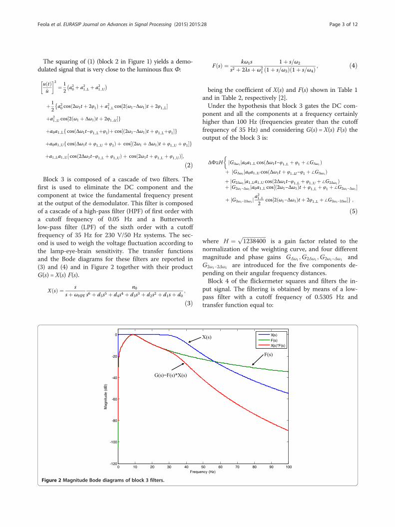
Block 3 is composed of a cascade of two filters. Thefirst is used to eliminate the DC component and thecomponent at twice the fundamental frequency presentat the output of the demodulator. This filter is composedof a cascade of a high-pass filter (HPF) of first order witha cutoff frequency of 0.05 Hz and a Butterworthlow-pass filter (LPF) of the sixth order with a cutofffrequency of 35 Hz for 230 V/50 Hz systems. The sec-ond is used to weigh the voltage fluctuation according tothe lamp-eye-brain sensitivity. The transfer functionsand the Bode diagrams for these filters are reported in(3) and (4) and in Figure 2 together with their productG(s) = X(s) F(s).

X sð Þ ¼ ssþ ωHPF

n0s6 þ d5s5 þ d4s4 þ d3s3 þ d2s2 þ d1sþ d0

;

ð3Þ

0 10 20 30 40-120

-100

-80

-60

-40

-20

0

Freque

)Bd(

edutingaM

G(s)=F(s)*X(s)

Figure 2 Magnitude Bode diagrams of block 3 filters.

F sð Þ ¼ kω1ss2 þ 2λsþ ω2

1

1þ s=ω2

1þ s=ω3ð Þ 1þ s=ω4ð Þ ; ð4Þ

being the coefficient of X(s) and F(s) shown in Table 1and in Table 2, respectively [2].Under the hypothesis that block 3 gates the DC com-

ponent and all the components at a frequency certainlyhigher than 100 Hz (frequencies greater than the cutofffrequency of 35 Hz) and considering G(s) = X(s) F(s) theoutput of the block 3 is:

ΔΦ≅H�

GΔω1j ja0a1 L cos Δω1t−φ1 L þ φ1 þ ∠GΔω1ð Þþ GΔω1j ja0a1 U cos Δω1t þ φ1 U−φ1 þ ∠GΔω1ð Þþ G2Δω1j ja1 La1 U cos 2Δω1t−φ1 L þ φ1 U þ ∠G2Δω1ð Þþ G2ω1−Δω1j ja0a1 L cos 2ω1−Δω1ð Þt þ φ1 L þ φ1 þ ∠G2ω1−Δω1½ �

þ G2ω1−2Δω1j j a21 L

2cos 2 ω1−Δω1ð Þt þ 2φ1 L þ ∠G2ω1−2Δω½ �g ;

ð5Þ

where H ¼ ffiffiffiffiffiffiffiffiffiffiffiffiffiffiffiffiffi1238400

pis a gain factor related to the

normalization of the weighting curve, and four differentmagnitude and phase gains GΔω1 ;G2Δω1 ;G2ω1−Δω1 andG2ω1−2Δω1 are introduced for the five components de-pending on their angular frequency distances.Block 4 of the flickermeter squares and filters the in-

put signal. The filtering is obtained by means of a low-pass filter with a cutoff frequency of 0.5305 Hz andtransfer function equal to:

50 60 70 80 90 100ncy (Hz)

X(s)

F(s)X(s)*F(s)

X(s)

F(s)

Table 1 Design parameter of X(s)

ωHPF n0 d0 d1 d2 d3 d4 d5

2π0.05 1.13 1014 1.13 1014 1.99 1012 1.75 1010 9.72 107 3.61 105 849.7

Feola et al. EURASIP Journal on Advances in Signal Processing (2015) 2015:28 Page 4 of 12

Y sð Þ ¼ 2π0:5305sþ 2π0:5305

: ð6Þ

This filter has the goal to attenuate all the sinusoidalcomponents, leaving the continuous component un-affected. Although the bandwidth of the filter is very nar-row, not all the sinusoidal components may be void. Forthis reason, the instantaneous flicker sensation due to thesingle interharmonic pair can be written as:

PU1 tð Þ ¼ PU1 DC þ PU1 AC tð Þ; ð7Þ

where PU1_DC and PU1_AC(t) are the DC and the residualAC component of the instantaneous flicker sensation,respectively.With reference only to the DC component of PU1 and

applying at the block 4 the signal (5), it is possible todemonstrate that:

PU1 DC ¼ PU1 DC1 þ PU1 DC2; ð8Þ

where PU1_DC1 and PU1_DC2 are equal, respectively, to:

PU1 DC1≅12H2 GΔω1j j2a20

� a21 L þ a21 U þ 2a1 La1 U cos φ1 L þ φ1 U−2φ1ð Þ ;

ð9Þ

PU1 DC2≅12H2

�G2Δω1j j2a21 La

21 U þ G2ω1þΔω1j j2a20a21 L

þ G2ω1þ2Δω1j j2 a41 L

4

�:

ð10Þ

As it will be shown in a more comprehensive mannerin the following sections, the first component (9) as-sumes prevalent values for all the values of Δω1 whilethe second (10) assumes values increasingly larger howclose is the frequency of the lower interharmonic toneto zero.It is worth noting that (9) corresponds to the analo-

gous expressions reported in [7] and in [10]. The differ-ence is that in cited references, the filter X(s) wasconsidered ideal, that is to say that G(s) = X(s)F(s) = F(s);so (9) considers the red curve of Figure 2 instead of thegreen one considered in [7] and in [10].

Table 2 Design parameter of F(s)

k λ ω1 ω2 ω3 ω4

1.74802 2π 4.05981 2π 9.15494 2π 2.27979 2π 1.22535 2π 21.9

With reference only to the residual AC component ofPU1 and applying at the block 4 the signal (5), it is pos-sible to demonstrate that:

PU1 AC tð Þ ¼ PU1 AC1 tð Þ þ PU1 AC2 tð Þ; ð11Þwhere PU1_AC1 and PU1_AC2, considering only the com-ponent of major interest, are equal, respectively, to:

PU1 AC1 tð Þ≅PU1 AC1 Δω1 tð Þ þ PU1 AC1 2Δω1 tð ÞþPU1 AC1 3Δω1 tð Þ þ PU1 AC1 4Δω1 tð Þ;

ð12ÞPU1 AC2 tð Þ≅PU1 AC2 2ω1−2Δω1ð Þ tð Þ

þPU1 AC2 4ω1−4Δω1ð Þ tð Þ:ð13Þ

PU1_AC1 and PU1_AC2 are oscillating components dueto the summation of sinusoidal signals with different an-gular frequencies (the angular frequency of each sum-mand is indicated in the subscript). In particular,PU1_AC1 assumes higher values how close Δω1 is to zero,while PU1_AC2 assumes higher values how close Δω1 isto the fundamental angular frequency.For the sake of brevity, the analytical assessment of

the summands of (12) and (13) are reported extensivelyin Appendix A.

2.2 Two pairsA normalized voltage with two pairs of superimposedinterharmonic tones in symmetrical frequency positions(Δω1 and Δω2) with respect to the fundamental signalcan be expressed as:

u tð Þu ¼ a0 cos ω1t þ φ1ð Þ þ a1 L cos ω1−Δω1ð Þt þ φ1 L½ �þa1 U cos ω1 þ Δω1ð Þt þ φ1 U½ �þa2 L cos ω1−Δω2ð Þt þ φ2 L½ �þa2 U cos ω1 þ Δω2ð Þt þ φ2 U½ �;

ð14Þwhere a1_L and a1_U and φ1_L and φ1_U represent therelative amplitudes and the phase angles of the firstinterharmonic pair, respectively, and a2_L and a2_Uand φ2_L and φ2_U of the second interharmonic pair,respectively.Using the same procedure used for the single pair of

interharmonic tones (shown in Section 2.1) and neglect-ing the effect on the AC component of the instantan-eous flicker sensation of the interaction between the twointerharmonic pairs, it is possible to demonstrate that:

Feola et al. EURASIP Journal on Advances in Signal Processing (2015) 2015:28 Page 5 of 12

PU1þ2 ¼ PU1 þ PU2 þ PU12 DC ¼ PU1 DC þ PU1 AC

þPU2 DC þ PU2 AC þ PU12 DC

¼ PU1 DC þ PU2 DC þ PU12 DCð Þþ PU1 AC þ PU2 ACð Þ

¼ PU1þ2 DC þ PU1þ2 AC;

ð15Þ

where PU1 and PU2 are obtained by means of (7) for theinterharmonic pair tones and PU12_DC is the DC com-ponent of instantaneous flicker sensation due to theinteraction between the two interharmonic pairs. Forsake of brevity, the analytical assessment of PU12_DC isreported in Appendix B. Again, as in (7), two differentcomponents, one DC (PU1+2_DC) and the other AC(PU1+2_AC), are defined.From the previous formulas, it should be noted that in

case of two interharmonic couples superimposed to the fun-damental signal, the PU is not only due to the sum of thecontributions to the instantaneous flicker sensation of thesingle interharmonic pair, but there is also a component dueto the combination effect of the interharmonic pairs. The en-tity of this effect will be evaluated in the following sections.

2.3 N pairsStarting from the analytical assessments of Section 2.2, itis possible to generalize the analytical assessment to thecase of N pairs of interharmonic tones. In fact, from(15), it is possible to obtain:

PUTOT ¼X∞j¼0

PUj þX∞j¼0

X∞k¼jþ1

PUkj DC

¼X∞j¼0

PUj DC þ PUj AC� �þX∞

j¼0

X∞k¼jþ1

PUkj DC

¼X∞j¼0

PUj DC1 þX∞k¼jþ1

PUkj DC

!þX∞j¼0

PUj AC

¼ PUTOT DC þ PUTOT AC;

ð16Þ

Time Domain Signal

IEC

Flickermeter

PUref

DFTAnalytical

Estimations

Figure 3 Block diagram of the numerical case studies.

where PUTOT_DC and PUTOT_AC are the DC andthe AC components, respectively, of the instantaneousflicker sensation due to N symmetric interharmonicpairs superimposed to the fundamental signal.

3 Numerical case studiesIn this section, different numerical case studies areshown to validate the analytical assessment presentedin Section 2. The results obtained by a numerical im-plementation of the IEC flickermeter (according withthe standard IEC 61000-4-15) and the results obtainedby the formulas of the analytical flickermeter pre-sented in this paper, both implemented in MATLAB,are compared. The block diagram of the numericalcase studies is shown in Figure 3.The steps performed to obtain the results of each nu-

merical case study are as follows:

1. A time domain signal with a length of 10 min withdifferent characteristics, according with the casestudy, is generated.

2. The signal is analysed by means of the IECflickermeter, which returns both the referenceof the instantaneous flicker sensation and ofthe short-term flicker severity value, PUref andPst_ref, respectively.

3. A DFT is performed only on the Fourier period ofthe signal-generated [1] since the signal is stationaryin terms of fundamental and interharmonic signalsin all the 10 min.

4. The output of the DFT is analysed by meansof the analytical formulas of Section 2,according with the case study, to obtain thevalue of instantaneous flicker sensation (PU).

5. The instantaneous flicker sensation is used asinput to the statistical evaluation (like thatdescribed in the Standard IEC 61000-4-15)to obtain the short-term flicker severity (Pst).

6. The values of PUref, Pst_ref, PU and Pst so obtainedhave been post-processed to calculate the error ofthe analytical estimation.

Pst_ref

PU Statistical

Evaluation

Pst

Pst Evaluation

Error

PU Evaluation

Error

0 5 10 15 20 25 30 35 40 45 500

1

2

3

4

5

6

7

8

Lower Interharmonic Frequency (Hz)

)%(

edutilpm

A

Figure 4 Amplitudes of pairs of symmetric interharmonics causing unitary Pst versus the pair lower interharmonic frequency.

Feola et al. EURASIP Journal on Advances in Signal Processing (2015) 2015:28 Page 6 of 12

3.1 Single pair producing AMThe interharmonic pairs have modulation frequenciesvarying between 0.1 and 49.9 Hz with steps of 0.1 Hz.For each modulation frequency, the amplitude of thepair taken from Figure 4, where the interharmonicamplitudes of pairs of symmetric interharmonic

0 5 10 15 20 250

5

10

15

20

25

30

35

40

Lower Interharmonic F

Pfo

noitamits

Eni

rorrE

st)

%(

X: 20.8Y: 5.157

X: 6.2Y: 5.368

X: 0.8Y: 5.734

BASEstP 1

IIIstP 1

IIstP 1

Figure 5 Percentage errors in estimation of Pst versus lower frequencPst. P

BASEst1 ; PIst1; P

IIst1 and PIIIst1 indicate the short-term flicker severity index con

the AC and the DC component of PU1 (17) (blue), only the DC component

tones superimposed to the fundamental causing a Pstequal to 1 versus the lower interharmonic frequencyof the pair, is shown. Furthermore, it should benoted that since the Fourier period of the signalgenerated is 10 s, a DFT with a spectral resolutionof 0.1 Hz is used.

30 35 40 45 50

X: 48.1Y: 5.051

requency (Hz)

X: 49.8Y: 3.671

PstBASE

PstI

PstII

PstIII

IstP 1

y of symmetric interharmonic pairs producing AM and unitarysidering, respectively, the analytical estimation proposed in [7] (cyan),of PU1 (18) (green) and only the PU1_DC1 component of PU1 (19) (red).

Feola et al. EURASIP Journal on Advances in Signal Processing (2015) 2015:28 Page 7 of 12

Three different analytical estimations of the instantan-eous Flicker sensation, with decreasing complexity, havebeen considered:

I) PUI1 ¼ PU1 ¼ PU1 DC1 þ PU1 DC2 þ PU1 AC; ð17Þ

II) PUII1 ¼ PU1 DC ¼ PU1 DC1 þ PU1 DC2; ð18Þ

III) PUIII1 ¼ PU1 DC1: ð19Þ

Obviously, the corresponding values of PIst1; P

IIst1 and

PIIIst1 have been calculated. Moreover, the results obtained

implementing the analytical assessment proposed in [7]are reported and referred to as PBASE

st1 .In Figure 5, the percentage errors (- PBASE

st1 - cyan curve, -

PUI1 - blue curve, - PUII

1 - green curve, - PUIII1 - red curve)

versus the lower interharmonic frequency of the symmetricinterharmonic pair are shown.From Figure 5, it is possible to observe the following:

� The blue curve PIst1

� �, in all the frequency range

analysed, gives the best results and only for thepair with the frequency of 49.9 Hz shows an errorgreater than 5% (black line). For this frequency,the error is caused mainly by the transientbehaviour of the filters contained in the IECflickermeter, which becomes non-negligible forinterharmonic frequencies very close to thefundamental. This transient behaviour is nottaken into account by pure frequency domainmethods differently from hybrid methods [12].

� The green curve PIIst1

� �and the red curve PIII

st1

� �are

virtually indistinguishable for frequencies greaterthan 15 Hz. Below this frequency (as mentioned inSection 2), the impact of PU1_DC2 on the total valueof PU1 is non-negligible, and for this reason, in thisfrequency range, the error committed by the analyticalestimation PII

st1 is less than that produced by PIIIst1.

� The PIIst1 estimation makes an error greater than 5%

(black line) for the pairs with frequencies higherthan 48 Hz and lower than 0.8 Hz. The reason ofthese errors (in addition to the previouslymentioned transient behaviour of the IECflickermeter for interharmonic frequencies veryclose to the fundamental) is due to the ACcomponent of PU1, which is more consistent forinterharmonic tones with Δω1 both close to thefundamental frequency or close to zero.

� The PIIIst1 estimation makes an error greater than 5%

(black line) for frequencies lower than 6.2 Hz andhigher than 48 Hz. The reasons of the differenttrend of the red curve with respect to the other two

curves are the same as the ones mentioned in theprevious point.

� The PBASEst1 (cyan curve) makes an error almost equal

to the PIIst1 and the PIII

st1 for frequencies higher than25 Hz, but for lower frequencies, as a result of thesimplifying assumptions, the error diverges, rapidlyreaching the 40% already for a frequency of 15 Hz.

3.2 Two pairs producing AMThe amplitude of the single pair of interharmonic tones hasbeen chosen to produce singly a Pst equal to 1 (Figure 4).The frequency modulation of the two pairs, which aredefined Δω1 and Δω2 in (14), has been chosen to vary be-tween 1 and 49 Hz, with steps of 1 Hz, and all their possiblecombinations have been evaluated. Since the Fourier periodof the input signal is equal to 1 s, a DFT with a spectralresolution of 1 Hz is used.Three different analytical estimations of the cumula-

tive Pst (Pst1+2) have been considered, all based on (15):

I)PUI1þ2 ¼ PU1þ2 ¼ PU1þ2 DC þ PU1þ2 AC: ð20Þ

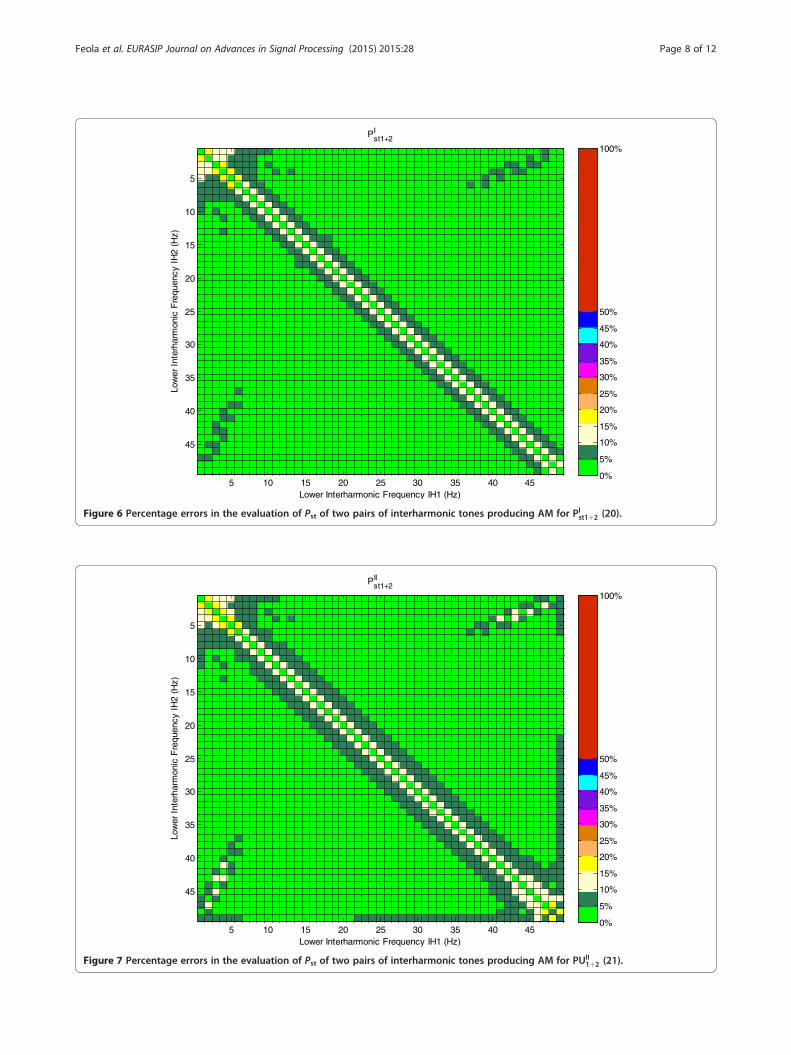
II) PUII1þ2 ¼ PU1þ2 DC: ð21Þ

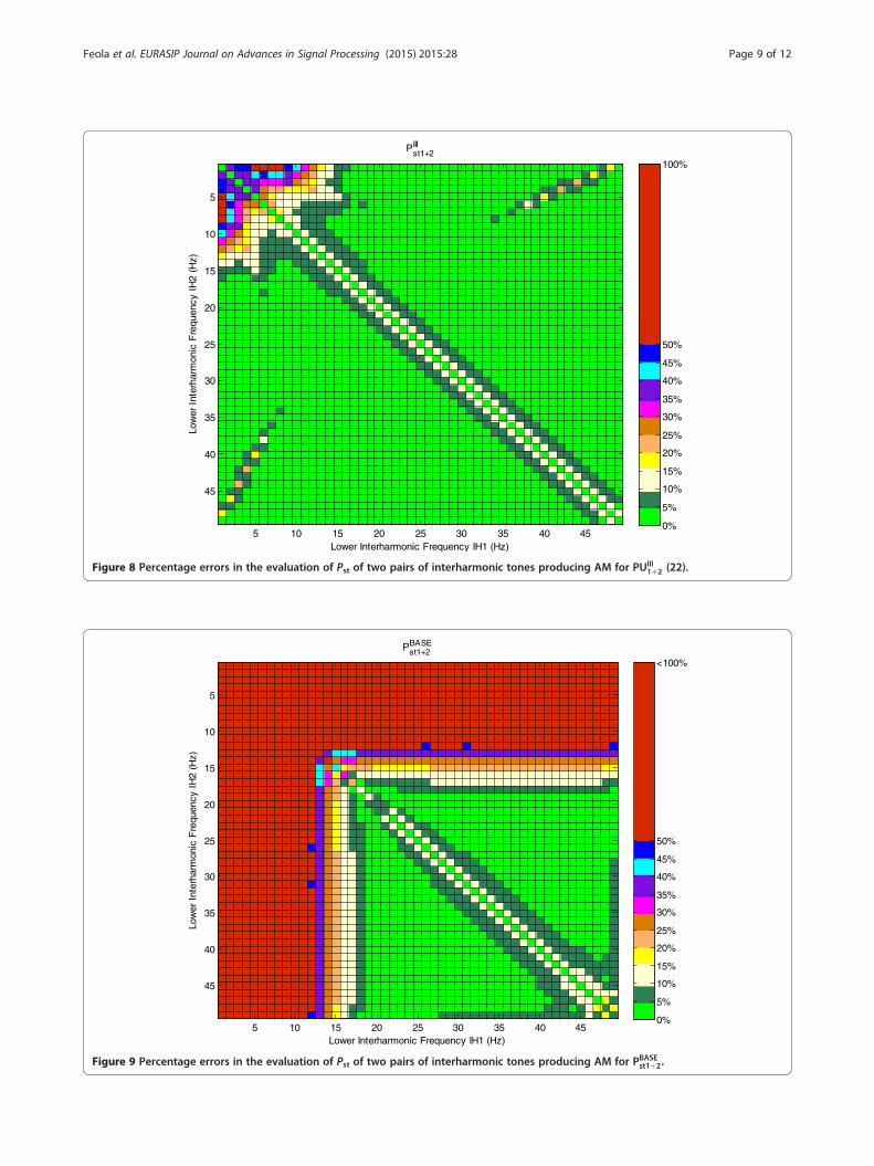
III) PUIII1þ2 ¼ PU1 þ PU2: ð22Þ

Obviously, the corresponding values of PIst1þ2; P

IIst1þ2

and PIIIst1þ2 have been calculated. Moreover, the results

obtained implementing the analytical assessment pro-posed in [7] are reported and referred to as PBASE

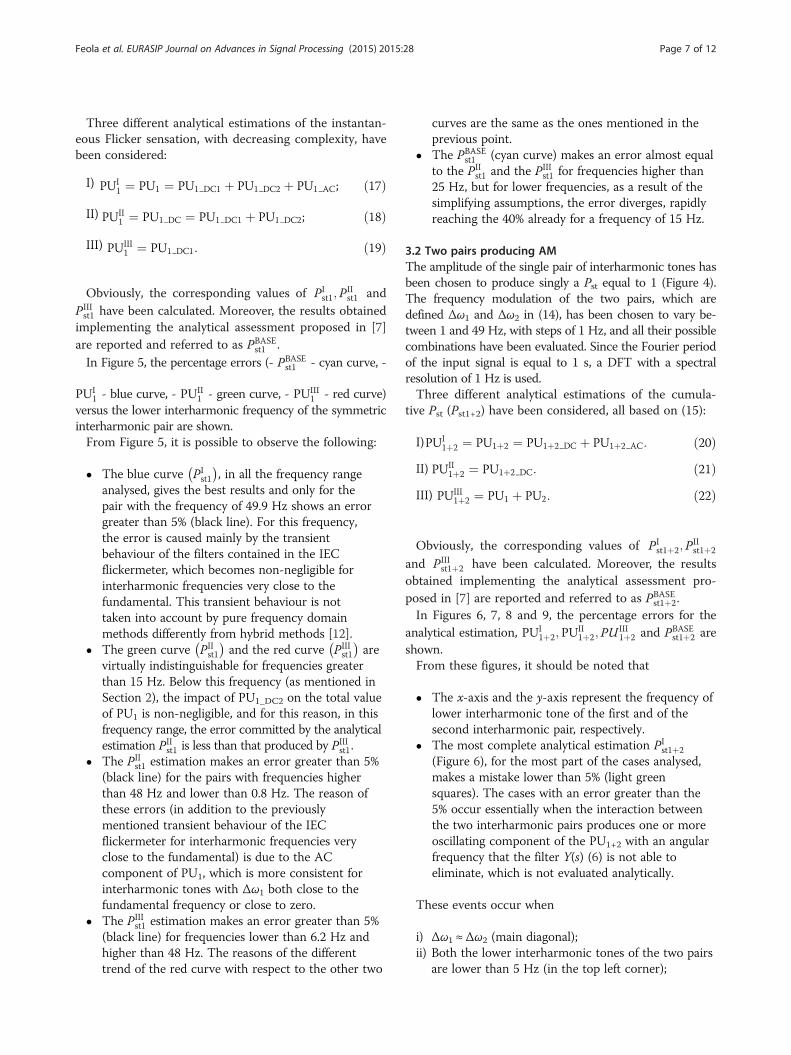
st1þ2.In Figures 6, 7, 8 and 9, the percentage errors for the

analytical estimation, PUI1þ2; PU

II1þ2; PU

III1þ2 and PBASE

st1þ2 areshown.From these figures, it should be noted that

� The x-axis and the y-axis represent the frequency oflower interharmonic tone of the first and of thesecond interharmonic pair, respectively.

� The most complete analytical estimation PIst1þ2

(Figure 6), for the most part of the cases analysed,makes a mistake lower than 5% (light greensquares). The cases with an error greater than the5% occur essentially when the interaction betweenthe two interharmonic pairs produces one or moreoscillating component of the PU1+2 with an angularfrequency that the filter Y(s) (6) is not able toeliminate, which is not evaluated analytically.

These events occur when

i) Δω1 ≈ Δω2 (main diagonal);ii) Both the lower interharmonic tones of the two pairs

are lower than 5 Hz (in the top left corner);

Lower Interharmonic Frequency IH1 (Hz)

)zH(

2HI

ycneuqerF

cinomrahretnI

rewoL

Pst1+2I

5 10 15 20 25 30 35 40 45

5

10

15

20

25

30

35

40

45

0%

5%

10%

15%

20%

25%

30%

35%

40%

45%

50%

100%

Figure 6 Percentage errors in the evaluation of Pst of two pairs of interharmonic tones producing AM for PIst1þ2 (20).

Lower Interharmonic Frequency IH1 (Hz)

)zH(

2HI

ycneuqerF

cinomrahretnI

rewoL

Pst1+2II

5 10 15 20 25 30 35 40 45

5

10

15

20

25

30

35

40

45

0%

5%

10%

15%

20%

25%

30%

35%

40%

45%

50%

100%

Figure 7 Percentage errors in the evaluation of Pst of two pairs of interharmonic tones producing AM for PUII1þ2 (21).

Feola et al. EURASIP Journal on Advances in Signal Processing (2015) 2015:28 Page 8 of 12

Lower Interharmonic Frequency IH1 (Hz)

)zH(

2HI

ycne uqe rF

cin omr ah retnI

rewoL

Pst1+2III

5 10 15 20 25 30 35 40 45

5

10

15

20

25

30

35

40

45

0%

5%

10%

15%

20%

25%

30%

35%

40%

45%

50%

100%

Figure 8 Percentage errors in the evaluation of Pst of two pairs of interharmonic tones producing AM for PUIII1þ2 (22).

Lower Interharmonic Frequency IH1 (Hz)

)zH(

2HI

ycn euqerF

cinomrahretnI

rewoL

Pst1+2BASE

5 10 15 20 25 30 35 40 45

5

10

15

20

25

30

35

40

45

0%

5%

10%

15%

20%

25%

30%

35%

40%

45%

50%

<100%

Figure 9 Percentage errors in the evaluation of Pst of two pairs of interharmonic tones producing AM for PBASEst1þ2.

Feola et al. EURASIP Journal on Advances in Signal Processing (2015) 2015:28 Page 9 of 12

Feola et al. EURASIP Journal on Advances in Signal Processing (2015) 2015:28 Page 10 of 12

iii)Δω1 ≈ 2(ω1 −Δω2) (in the top right corner);iv)Δω2 ≈ 2(ω1 −Δω1) (in the bottom left corner).

� Comparing the results obtained for PIst1þ2

(Figure 6) and for PIIst1þ2 (Figure 7), it should be

noted that neglecting the effects of the ACcomponents produced by the singleinterharmonic pair increases the number of non-light green squares when

i) Δω1 ≈ Δω2 (main diagonal);ii) Δω1 ≈ 2(ω1 −Δω2) (in the top right corner) and

when Δω2 ≈ 2(ω1 −Δω1) (in the bottom left corner);iii)Δω1 = 1 (last column to the right) and when Δω2 = 1

(last column to the bottom).

� Comparing the results obtained for PI

st1þ2(Figure 6) and for PIII

st1þ2 (Figure 8), it should benoted that neglecting the effects of theinteractions between the two interharmonic pairson the DC component of the PU1+2 are presentwith a non-negligible entity when

i) Both the pairs have the lower interharmonic tonefrequency lower than 15 Hz (in the top left corner);

ii) Δω1 = 2(ω1 − Δω2) (in the top right corner) or whenΔω2 ≈ 2(ω1 −Δω1) (in the bottom left corner).

� In similar mode to the case of an interharmonic

pair shown in Figure 5, the analytical assessmentPBASEst1þ2 (Figure 9) makes errors very high

(sometimes even more than 100%) when oneor both the pairs have the lower interharmonictone with frequencies lower than 20 Hz.

� Finally, it is worthwhile to note that from theimplementation point of view on a general PQinstrument, the proposed analytical approachrequires only some manipulations, of differentcomplexities depending on the level ofapproximation desired (see (20), (21) and (22)),of the spectra which are already evaluated bythe PQ instrument for the harmonic andinterharmonic analysis. On the other hand, thedigital signal processing of the conventional IECflickermeter requires the implementation of blocks1 to 4 independently from the spectral analysis.

4 ConclusionsIn this paper, a new analytical estimator for LF in the fre-quency domain, which is able to take into account alsothe frequency components neglected by the classicalmethods proposed in literature, has been proposed. Theanalytical solutions proposed apply for any generic sta-tionary signal affected by interharmonic distortion. TheLF analytical estimator proposed has been applied tonumerous numerical case studies with the goal of showingi) the correctness and the improvements of the analytical

approach proposed in respect with the other method pro-posed in literature and ii) the accuracy of the results com-pared to those obtained by means of the classical IECflickermeter. The usefulness of the proposed analytical ap-proach is that it can be included in signal processing toolsfor interharmonic penetration studies for the integrationof renewable energy sources in future smart grids.The main outcomes of the paper are as follows:

� In the presence of interharmonic tones in thefrequency range from DC to 15 Hz and from 85to 100 Hz, the simplified assumptions made byclassical methods proposed in literature can leadto very inaccurate results.

� The analytical formulas can be used to performinterharmonic penetration studies in transmissionand distribution networks.

Future development of the research will be aimed togeneralize the methodology adapted to interharmoniccomponents at frequencies higher than 100 Hz which isproven to affect modern lighting systems different fromincandescent bulbs.

5 Appendix A Analytical assessment of PU1_AC(t)With reference to (11), it is possible to demonstrate thatthe summands of (12) are equal to the following:

PU1 AC1 Δω1 tð Þ≅H2 YΔω1j j2

f 2 GΔω1j j G2Δω1j ja0a21 La1 U cosðΔω1t

þφ1 U−φ1−∠GΔω1 þ ∠G2Δω1 þ ∠Y Δω1Þþ 2 GΔω1j j G2Δω1j ja0a1 La

21 U cos

�Δω1t−φ1 L

þφ1−∠GΔω1 þ ∠G2Δω1 þ ∠YΔω1Þþ G2ω1−2Δω1j j G2ω1−Δω1j ja0a31 L cos

�Δω1t−φ1 L

þφ1−∠G2ω1−2Δω1 þ ∠G2ω1−Δω1 þ ∠YΔω1Þg;ð23Þ

PU1 AC1 2Δω tð Þ≅H2

2Y 2Δω1j j GΔω1j j2a20½ a21 L cosð2Δω1t−2φ1 L

þ2φ1 þ 2∠GΔω1 þ ∠Y 2Δω1Þ þ a21 U cosð2Δω1t

þ2φ1 U þ 2φ1−2∠GΔω1 þ ∠Y 2Δω1Þþ2a1 La1 U cos

�2Δω1t−φ1 L þ φ1 U þ 2∠GΔω1

þ∠Y 2Δω1Þ�;ð24Þ

PU1 AC1 3Δω1 tð Þ≅H2 Y 3Δω1j j GΔω1j j G2Δω1j ja0�½a21 La1 U cosð3Δω1t−2φ1 L þ φ1 U−φ1þ∠GΔω1 þ ∠G2Δω1 þ ∠Y 3Δω1Þþa1 La21 U cosð3Δω1t þ 2φ1 U−φ1 L−φ1þ∠GΔω1 þ ∠G2Δω1 þ ∠Y 3Δω1Þ�;

ð25Þ

Feola et al. EURASIP Journal on Advances in Signal Processing (2015) 2015:28 Page 11 of 12

PU1 AC1 4Δω1 tð Þ≅H2

2Y 4Δω1j j G2Δω1j j2a21 La

21 U cosð4Δω1t−2φ1 L

þ2φ1 U þ 2∠G2Δω1 þ ∠Y 4Δω1Þ;ð26Þ

and that the summands of (13) are equal to the following:

PU1 AC2 2ω1−2Δω1 tð Þ≅H2 Y 2ω1−2Δω1j j GΔω1j j G2ω1−Δω1j ja20fa21 L cos½2 ω1−Δω1ð Þt þ 2φ1 L−∠GΔω1

þ∠G2ω1−Δω1 þ ∠Y 2ω1−2Δω1 �þ a1 La1 U cos½2 ω1−Δω1ð Þt þ φ1 L−φ1 U

þ2φ1−∠GΔω1 þ ∠G2ω1−Δω1 þ ∠Y 2ω1−2Δω1 �gð27Þ

PU1 AC2 4ω1−4Δω1 tð Þ≅H2

8Y 4ω1−4Δω1j j G2ω1−2Δω1j j2a41 L cos½4 ω1−Δω1ð Þt

þ4φ1 L þ 2∠G2ω1−2Δω1 þ ∠Y 4ω1−4Δω1 �;ð28Þ

6 Appendix B Analytical Assessment of PU12_DC

With reference to (15), PU12_DC can be expressed as:

PU12 DC ¼ PU12 DC1 þ PU12 DC2: ð29Þ

It is possible to demonstrate that PU12_DC1 is equal to:

PU12 DC1 ¼ 12H2f G2ω1−Δω1−Δω2j j2a21 La

22 L

þ G2ω1−Δω1þΔω2j j2a21 La22 U

þ G2ω1þΔω1−Δω2j j2a21 Ua22 L

þ GΔω1þΔω2j j2½a21 Ua22 L þ a21 La

22 U

þ2a1 La1 Ua2 La2 U cosðφ1 L

þφ1 U−φ2 L−φ2 LÞ�þ GΔω1−Δω2j j2½a21 La

22 L þ a21 Ua

22 U

þ2a1 La1 Ua2 La2 U cosðφ1 L

þφ1 U−φ2 L−φ2 LÞ�g;

ð30Þ

and that PU12_DC2, considering Δω1 >Δω2, assumes dif-ferent values according to the relationship between Δω1

and Δω2:

� For 3Δω1 −Δω2 = 2ω1, it is equal to:

PU12 DC2 ¼ 12H2f GΔω1−Δω2j j2½a31 La2 L cos 3φ1 L−φ2 Lð Þ

þa21 La1 Ua2 U cos 2φ1 L−φ1 U þ φ2 Uð Þ�þ2 G2Δω1j j2a1 La

21 Ua2 L cos −φ1 L−φ2 Lð Þg;

ð31Þ

� For Δω2 + 2Δω1 = 2ω1, it is equal to:

PU12 DC2 ¼ 12H2f GΔω2j j2½a2 La

21 La cosð−φ2 L−2φ1 L

þφÞ þ a2 Ua21 La cos φ2 U−2φ1 L þ φð Þ�

þ2 GΔω1þΔω2j j2½a1 La1 Ua2 La cosðφ1 L−φ1 U

þφ2 L þ φÞ þ a21 La2 Ua cos 2φ1 L−φ2 U þ φð Þ�þ2 GΔω1j j2½a2 La

21 La cosð−φ2 L−2φ1 L þ φÞ

þa1 La2 La1 Ua cosð−φ1 L−φ2 L þ φ1 U−φÞ�þ2 G2Δω1j j2a2 La1 La1 Ua cosð−φ2 L−φ1 Lþφ1 U−φÞg;

ð32Þ

� For Δω1 = 2Δω2, it is equal to:

PU12 DC2 ¼ 12H2f 2 GΔω1j j2½a1 La2 La2 Ua cosð−φ1 L þ φ2 L−φ2 U

þφÞ þ a1 Ua2 La2 Ua cosðφ1 U þ φ2 L−φ2 U−φÞ�þ2 GΔω2j j2½a1 La

22 La cos þφ1 L−2φ2 L þ φð Þ

þa1 Ua2 La2 Ua cosð−φ1 U−φ2 L þ φ2 U

þφÞ þ a1 La2 La2 Ua cos φ1 L−φ2 L þ φ2 U−φð Þþa1 Ua

22 Ua cosð−φ1 U þ 2φ2 U−φÞ�

þ2jG2ω1−Δω1þΔω2 j2a1 La2 La2 Ua cosð−φ1 L

þφ2 L−φ2 U þ φÞ þ G2ω1−2Δω2j j2a1 La22 La

cos −φ1 L þ 2φ2 L−φð Þg:ð33Þ

Competing interestsThe authors declare that they have no competing interests.

AcknowledgementsThe research activity discussed in this paper has been partially supported bythe Project PON01_02582 “Command, control, protection and supervisionintegrated system for production, transmission and distribution (ColAdMinintegrated SCADA) of renewable and non renewable electrical energy,with field-device-interface, for rational use of electrical power” funded bythe Italian Ministry for the Instruction, University and Research.

Received: 15 December 2014 Accepted: 16 February 2015

References1. IEEE Task, Force on harmonics modeling and simulation, interharmonics:

theory and modeling. IEEE Trans. Power Deliv. 22(4), 2335–2348 (2007).doi:10.1109/TPWRD.2007.905505

2. IEC Standard 61000-4-15. Flickermeter—functional and design specifications(IEC, Geneva, Switzerland, Edition 2.0, 2010-07)

3. R Langella, A Testa, Amplitude and phase modulation effects of waveformdistortion in power systems. J. Electrical Power Qual. Util. XIII(1), 25–32 (2007)

4. D Gallo, R Langella, A Testa, Light Flicker Prediction Based on Voltage SpectralAnalysis (Paper presented at the IEEE Porto Power Tech Conference, Porto,Portogallo, 2001), pp. 10–13

5. R Langella, A Testa, Power System Subharmonics, ed. by IEEE (Paper invitedat the IEEE Power Engineering Society General Meeting 2005, S. Francisco,USAm, 2005)

6. T Keppler, NR Watson, S Chen, J Arrilaga, Digital flickermeter realisations inthe time and frequency domains, ed. by Australasian Committee for PowerEngineering (Paper presented at the Australasian Power EngineeringConference, Perth, Australia, September, 2001)

Feola et al. EURASIP Journal on Advances in Signal Processing (2015) 2015:28 Page 12 of 12

7. A Hernandez, JG Mayordomo, R Asensi, LF Beites, A new frequency domainapproach for flicker evaluation of arc furnaces. IEEE Trans. Power Deliv.18(2), 631–638 (2003). doi:10.1109/TPWRD.2003.809733

8. CJ Wu, TH Fu, Effective voltage flicker calculation algorithm using indirectdemodulation method. IEE P-Gener. Transm. D. 150(4), 493–500 (2003).doi:10.1049/ip-gtd:20030302

9. T Keppler, NR Watson, J Arrilaga, S Chen, Theoretical assessment of lightflicker caused by sub- and interharmonic frequencies. IEEE Trans. PowerDeliv. 18(1), 329–333 (2003). doi:10.1109/TPWRD.2002.806690

10. D Gallo, R Langella, C Landi, A Testa, On the use of the flickermeterto limit low-frequency interharmonic voltages. IEEE Trans. Power Deliv.23(4), 1720–1727 (2008). doi:10.1109/TPWRD.2008.2002842

11. N Kose, O Salor, New spectral decomposition based approach for flickerevaluation of electric arc furnaces. IET Gener. Transm. Dis. 3(4), 393–411(2009). doi:10.1049/iet-gtd.2008.0479

12. GW Chang, C Cheng-I, H Ya-Lun, A digital implementation of flickermeterin the hybrid time and frequency domains. IEEE Trans. Power Deliv.24(3), 1475–1482 (2009). doi:10.1109/TPWRD.2009.2022673

13. A Hernández, JG Mayordomo, R Asensi, LF Beites, A method based oninterharmonics for flicker propagation applied to arc furnaces. IEEE Trans.Power Deliv. 20(3), 2334–2342 (2005). doi:10.1109/TPWRD.2005.848677

14. IEC standard 61000-4-7: General guide on harmonics and interharmonicsmeasurements, for power supply systems and equipment connectedthereto (IEC, Geneva, Switzerland, Edition 2.0, 2002-08)

15. K Yang, MHJ Bollen, EO Anders Larsson, M Wahlberg, Measurements ofharmonic emission versus active power from wind turbines. Electr. Pow.Syst. Res. 108, 304–314 (2014). doi:10.1016/j.epsr.2013.11.025

16. F De Rosa, R Langella, A Sollazzo, A Testa, On the interharmoniccomponents generated by adjustable speed drives. IEEE Trans. Power Deliv.20(4), 2535–2543 (2005). doi:10.1109/TPWRD.2005.852313

17. R Carbone, F De Rosa, R Langella, A Testa, A new approach for thecomputation of harmonics and interharmonics produced by line-commutated AC/DC/AC converters. IEEE Trans. Power Deliv.20(3), 2227–2234 (2005). doi:10.1109/TPWRD.2005.848448

18. R Langella, A Sollazzo, A Testa, A new approach for the computation ofharmonics and interharmonics produced by AC/DC/AC conversion systemswith PWM inverters. Eur. T. Electr. Power 20(1), 68–82 (2010). doi:10.1002/etep.400

Submit your manuscript to a journal and benefi t from:

7 Convenient online submission

7 Rigorous peer review

7 Immediate publication on acceptance

7 Open access: articles freely available online

7 High visibility within the fi eld

7 Retaining the copyright to your article

Submit your next manuscript at 7 springeropen.com