A New Keynesian Model with Staggered Price and Wage Setting under Learning Gabriela Best 1 Abstract This paper provides a study of the implications for economic dynamics when the central bank sets its nominal interest rate target in response to variations in wage inflation. I provide results on the existence, uniqueness, and stability under learning of rational expectations equilibrium for alternative specifica- tions of the manner in which monetary policy responds to economic shocks when nominal rigidities are present. Monopolistically competitive producers set prices via staggered price contracts, and households set nominal wages in the same fashion. In this setting, the conditions for determinacy and learnability of rational expectations equilibrium differ from a model where only prices are sticky. I find that when the central bank responds to wage and price inflation and to the output gap, a Taylor principle for wage and price inflation arises that is related to stability under learning dynamics. In other words, a moderate reaction of the interest rate to wage inflation helps to avoid instability under learning and indeterminacy. Keywords: Learning, Monetary Policy, Nominal Wage and Price Rigidity, Expectational stability. JEL classification: E52, E31, E43, E58. 1. Introduction The New Keynesian model has become a workhorse for the study of monetary policy in recent years. In this model, the behavior of private agents depends not only on current policy but also on the expected course of monetary policy. Mone- tary models typically assume that authorities adopt either linear feedback monetary rules (Taylor-type rules) or optimal monetary policy rules in an attempt to control Email address: [email protected](Gabriela Best) 1 California State University, Fullerton, Department of Economics, Steven G. Mihaylo College of Business and Economics, Fullerton, CA 92834-6848. Telephone: (657) 278-2387; fax: (657) 278-3097. Preprint submitted to Journal of Economic Dynamics and Control May 27, 2015
Transcript
A New Keynesian Model with Staggered Price and WageSetting under Learning
Gabriela Best1
Abstract
This paper provides a study of the implications for economic dynamics whenthe central bank sets its nominal interest rate target in response to variationsin wage inflation. I provide results on the existence, uniqueness, and stabilityunder learning of rational expectations equilibrium for alternative specifica-tions of the manner in which monetary policy responds to economic shockswhen nominal rigidities are present. Monopolistically competitive producersset prices via staggered price contracts, and households set nominal wagesin the same fashion. In this setting, the conditions for determinacy andlearnability of rational expectations equilibrium differ from a model whereonly prices are sticky. I find that when the central bank responds to wageand price inflation and to the output gap, a Taylor principle for wage andprice inflation arises that is related to stability under learning dynamics. Inother words, a moderate reaction of the interest rate to wage inflation helpsto avoid instability under learning and indeterminacy.
The New Keynesian model has become a workhorse for the study of monetarypolicy in recent years. In this model, the behavior of private agents depends notonly on current policy but also on the expected course of monetary policy. Mone-tary models typically assume that authorities adopt either linear feedback monetaryrules (Taylor-type rules) or optimal monetary policy rules in an attempt to control
Email address: [email protected] (Gabriela Best)1California State University, Fullerton, Department of Economics, Steven G. Mihaylo
College of Business and Economics, Fullerton, CA 92834-6848. Telephone: (657) 278-2387;fax: (657) 278-3097.
Preprint submitted to Journal of Economic Dynamics and Control May 27, 2015
the economy. However, the role of said rules in stabilizing the economy has beencriticized because of their potential to induce indeterminacy or very large sets ofrational expectations equilibria. If the central bank follows a rule that leads to mul-tiple equilibria, agents might be incapable of coordinating on a specific equilibrium;even when capable of such coordination, this equilibrium might not be targeted bythe central bank due to its undesirable characteristics.2
Alternatively, under certain conditions, agents can “learn” the desirable equi-librium targeted by the central bank and eventually converge to the rational expec-tations equilibrium (REE). Agents “learn” the equilibrium of the model by makingforecasts based on recursive least squares techniques and the data obtained fromthe economy. These forecasts replace rational expectations (RE) in the model. Inthis context, the expectational stability (E-stability) concept discussed in Evansand Honkapohja (1999) and (2001) is applied in order to determine whether ratio-nal expectations equilibria are stable under learning dynamics.3 When equilibriaare E-stable, even when there are discrepancies between the agents’ expectationsand expectations required to yield a determinate REE, the system will converge tothe REE. Therefore, designing rules that lead to learnable equilibria is desirable.Evans and McGough (2005a) studied determinacy and learnability conditions asselection criteria. Bullard and Mitra (2002, BM hereafter), derived determinacyand learnability conditions for monetary policy linear feedback rules, and Evansand Honkapohja (2003) determine the same conditions for optimal rules.4 Othershave examined them for open-economy models.5
Recent work has shown that staggering of nominal wage contracts is impor-tant to give rise to the key frictions that render monetary policy non-neutral. Infact, Christiano et al. (2005) conclude that wage stickiness—not price stickiness—appears more important in explaining output and inflation dynamics. Models thatconsider only sticky prices and not sticky wages have been criticized for producing“too sharp a real-wage decline in response to a tightening of monetary policy” as
2The large multiplicity of solutions and its harmful implications including equilibriumresponses to shocks to fundamentals and sunspot states that could lead to arbitrarilylarge fluctuations in endogenous variables, have been widely discussed in Bullard andMitra (2002), and Woodford (1999) and (2003).
3“Learnability,” “E-stability,” “stability under learning” are synonyms in the currenttext.
4They propose that central banks should adopt an optimal policy rule that includesboth expectations and fundamentals to ensure determinacy and learnability of the REE.
5Authors include Llosa and Tuesta (2008), Bullard and Schaling (2009), Bullard andSingh (2008), Zanna (2009), and Wang (2006). These authors examine rules that respondto exchange rate movements. Moreover, extensions of the model that consider determinacyand Expectational stability of REE when long-term interest rates are included in the modelare studied in McGough et al. (2005), and Kurozumi and Van Zandweghe (2008). Duffyand Xiao (2011) and Pfajfar and Santoro (2012) examine these rules in the context ofmodels featuring physical capital. Evans and Honkapohja (2009) provide a comprehensiveoverview of recent literature on expectations, learning, and monetary policy.
2
addressed in Christiano et al. (1999). Christiano et al. (2005), Altig et al. (2011),and Smets and Wouters (2007) further conclude that impulse response functions af-ter a monetary policy shock are best fit by the model with staggered wage contracts.This explanation validates wage stickiness as an important factor in explaining thereal effects of monetary policy.
BM evaluate alternative monetary policy rules in the context of determinacyand E-stability in a standard New Keynesian model under price rigidity but wageflexibility. The authors conclude that the equilibria can be learnable when thecentral bank raises its interest rate instrument more than one-for-one with increasesin inflation. This condition is referred to the “Taylor principle condition.” It isnot obvious that an optimizing-agent model with staggered nominal wage settingin addition to staggered price setting would yield determinacy and expectationalstability (E-stability) conditions similar to a model in which only prices are sticky.One reason is that the volatility of aggregate wage inflation induces inefficienciesin the distribution of employment across households (Erceg et al., 2000). For thatreason, this paper builds on BM and develops a comprehensive and systematicstudy of the determinacy and E-stability properties of the New Keynesian modelunder both price and wage rigidity. In particular, its contribution is to evaluatethe E-stability properties of different monetary policy rules that embed an explicitresponse to wage inflation. Previous studies had concentrated only on documentingthe determinacy properties of the staggered prices and wages model (see, e.g.,Flaschel et al., 2008; and Franke and Flaschel, 2009; Galı, 2008). Galı (2008),through a numerical experiment, finds that if the interest rate reacts more thanone to one to contemporaneous price inflation or wage inflation, then the REE isdeterminate. Flaschel et al. (2008) and Franke and Flaschel et al. (2009) confirmthis result analytically by reformulating the model in continuous time.
This paper also relates to Huang et al. (2009), Ascari et al. (2011), andCarlstrom and Fuerst (2007), who study wage rigidities as a “special case” of theirmodels. Huang et al. (2009) initially present a sticky price model with endogenousinvestment and find that incorporating both sticky wages and firm-specific capitalmakes the determinacy region quite large. Carlstrom and Fuerst (2007) analyzewhether monetary policy should respond to asset prices in a model with price andwage stickiness from the point of view of equilibrium determinacy. They concludethat equilibra are likely to be indeterminate when the central bank adjusts policyin response to asset price movements. Lastly, Ascari et al. (2011) present anestimated monetary policy rule that includes a time-varying trend inflation andstochastic coefficients in a New Keynesian model for the U.S. economy and studyits determinacy properties. Results suggest that including wage stickiness makesthe determinacy region very sensitive to trend inflation. However, none of thesepapers focus on E-stability in the presence of wage stickiness.
The analysis presented in this paper views the short-term interest rate as theinstrument of monetary policy design. The policy-design problem lies in character-izing how the interest rate should respond to changes in wage and price inflationto induce a learnable equilibrium given that both prices and wages exhibit rigidi-ties. Wage inflation provides information about the rate of core inflation (De Long,
3
1997). Having a central bank that targets wage inflation in its policy rule is desir-able because such rules (i) are welfare enhancing, performing nearly as well as theoptimal rule, (Casares, 2007; Canzoneri et al., 2005; Erceg et al., 2000; Levin et al.,2006; Marzo, 2009)6; (ii) are simple (Levin et al., 2006) and have a good empiricalfit to the data (Casares, 2007); and (iii) maximize economic stability (Mankiw andReis, 2003). The underlying reason why wage inflation targeting is so desirable inthe presence of price and wage rigidities is that wage rigidities create cross-sectionalwage dispersion across households, which leads to inefficiencies in hiring decisions.In this setting, the cost of aggregate employment volatility is amplified. Stabilizingwage inflation eases wage dispersion and decreases the inefficiencies in employment.
The main results of this paper are twofold. First, a Taylor principle condition forwage and price inflation emerges when the central bank responds to wage inflation,price inflation, and the output gap. When the central bank adjusts its interest ratespositively and more than one for one with changes in price and/or wage inflationabove target, a “leaning against the wind” policy is followed. If agents do nothave RE and they form forecasts using least squares learning, then such policyfrom the central bank pushes the equilibrium toward the REE. Thus, a leaningagainst the wind policy for a combination of wage and price inflation when agentsform forecasts using least squares learning is closely linked to learnable equilibria.This result holds when interest rates respond to current data and forward-lookingexpectations. Second, there are instances in which having a central bank thatresponds mainly to wage inflation is preferable to responding to price inflation inits policy rule. Specifically, if the relative role of wage stickiness is more importantin practice than the role of price stickiness, responding primarily to wage inflationin the policy rule results in a larger determinacy and E-stability regions of theparameter space. Responding to wage inflation, in this setting, relaxes the upperbound constraint on the response to wage inflation that appears in forward lookingand lagged rules which ensures determinacy and E-stability.
From a welfare theoretic perspective, Erceg et al. show that the welfare costof wage inflation volatility increases with the mean duration of wage contracts.They advocate implementing mixed rules that respond to wage and price inflation.To conclude, the result presented here supports Erceg et al. (2000) and Mankiwand Reis (2003) in the sense that it is desirable to design rules that respond to acombination of price and wage inflation due to their potential to induce determinacyand E-stability.
The rest of this paper is structured as follows. Section 2 presents the model,the alternative policy rules studied under the analysis, and the general conditionsfor E-stability akin to the model. Section 3 presents results on determinacy andlearnability of equilibrium under alternative policy rules for a model with wage andprice stickiness. Section 4 concludes.
6When the policymaker strictly targets price inflation in a model that includes stag-gered wage setting, there is a considerably large welfare loss due to substantial variationin the nominal wage inflation and the output gap.
4
2. The Environment
2.1. The Model
The structural equations of the supply side of the model are from Woodford(2003) (chapter 8, section 2.2), as follows:
πt = β Etπt+1 + κp(xt + ut) + ξp(wt − wnt ), (1)
πwt = β Etπwt+1 + κw(xt + ut) + ξw(wnt − wt), (2)
wt = wt−1 + πwt − πt, (3)
where κp ≡ ξpωp and κw = ξw(ωw + σ−1), where ξp =(1−αp)(1−αpβ)αp(1+ωpθp)
and ξw =(1−αw)(1−αwβ)αw(1+vθw) .
Here πwt is nominal wage inflation, wt is the log real wage, wnt represents ex-ogenous variation in the natural real wage, xt is the output gap, ut is treated as anexogenous i.i.d. shock with variance σ2
u, and E represents (possibly nonrational)expectations. The terms ξp, ξw, κp, and κw are all positive. Prices and wages areadjusted a la Calvo, where 1−αp (1−αw) is the time-independent probability thateach of the prices (wages) is adjusted each period. The parameter ξp represents thesensitivity of goods-price inflation to changes in the average gap between marginalcost and current prices; it is smaller as prices are stickier (αp). The parameter ξwindicates the sensitivity of wage inflation to changes in the average gap betweenhouseholds’ “supply wage” (the marginal rate of substitution between labor supplyand consumption) and current wages, and it is a function of the Calvo parameterthat denotes wage stickiness in the economy (αw). ωp > 0 represents the elasticityof supply wage with respect to the quantity supplied at a given wage, while ωw > 0measures the elasticity of the supply wage with respect to the quantity produced;holding fixed households’ marginal utility of income, σ > 0 is the inverse of theintertemporal elasticity of substitution. Eqs. (1) and (2) are Phillips curves forprices and wages. Eq. (3) is an identity for the real wage (wt = Wt/Pt) expressedin logs and was rearranged in this form to provide a law of motion for the log ofnominal wages.
The dynamic IS-type equation is described by
xt = Etxt+1 − σ(it − Etπt+1 − rnt ), (4)
where it is the nominal interest rate and rnt is an exogenous i.i.d. shock with varianceσ2rn .7 Monetary policy is represented by a Taylor-type rule that responds to price
7The exogenous shock rnt has been defined as an exogenous stochastic term that followsan AR(1) process in previous literature. This specification could potentially impact theE-stability conditions of the model. I abstain from this representation to avoid furthercomplications in the derivation of the E-stability conditions of the model.
5
inflation, wage inflation, and the output gap. The monetary policy parameters aredenoted by ψπw , ψπ, and ψx. The baseline specification is
it = ψππt + ψπwπwt + ψxxt. (5)
This will be called the contemporaneous data specification because policymakersrespond to contemporaneous data in their policy rules, and only the private sectorforms expectations about future values of endogenous variables. The model con-sists of Eqs. (1)− (5), they represent log-linear approximations of the equilibriumconditions outlined in Woodford (2003) and characterize only equilibria involvingfluctuations around a zero inflation steady state.
2.2. Alternative Policy Rule SpecificationsIn addition to the baseline specification, I explore the determinate and E-stable
regions of the parameter space when policymakers respond to possibly nonrationalexpectations of the policy variables, and lagged data in the policy rule with andwithout policy inertia. The first two specifications pertain to the cases withoutpolicy inertia:
This specification includes a policy function where the interest rate respondsto current forecasts of one-quarter-ahead output gap, price inflation rate, and wageinflation rate. Forecast based rules describe well the conduction of monetary policyfor the United States after 1979 as described in Best and Kapinos (2015) and Galiand Gertler (1998). This forward-looking policy function is represented by
where the term ψi = 0. The model now consists of Eqs. (1)-(4), and Eq. (5) isreplaced by Eq. (6).
Alternatively, the central bank is more likely to respond to past data of thevariables included in the policy function because contemporaneous data from thequarter in which they need to make policy decisions are rarely available. Specifically,the central bank has readily available data from the past quarter to which theinterest rate should respond. For that reason, I include a policy function thatresponds to last-quarter data of the output gap, price inflation, and wage inflation.Equation (5) is now replaced by
it = ψππt−1 + ψπwπwt−1 + ψxxt−1 + ψiit−1. (7)
where ψi has also been set to 0.As has been widely addressed in the literature (Bullard and Mitra, 2007; Dennis,
2006; Evans and McGough, 2005c; Cukierman, 1989; and Brainard, 1967), rulesthat respond cautiously to inadvertent changes in economic conditions are desirable.This caution can be modeled by having a central bank that responds to inertia onits policy rule. Equation (6) presents a forward-looking policy function with policyinertia in which the interest rate instrument responds to changes in the forecastsof price and wage inflation, and the output gap, as well as the lagged interest rate.Alternatively, Eq. (7) represents a policy rule in which the central bank respondsnot only to lagged variables, but also to a lagged interest rate term.
6
2.3. Determinacy
RE are viewed as a two-sided equilibrium in which expectations influence thetime path of the economy and the time path of the economy affects expectations.A model is said to be determinate if it has a unique dynamically stable REE. Thegeneral conditions for determinacy are outlined below. Consider a general class ofmodels:
yt = α+BEtyt+1 + δyt−1 + κet (8)
where yt is an n × 1 vector of endogenous variables; et is a vector of white noise;and B, δ, and κ are n× n matrices of coefficients.
For determinacy analysis the δ matrix in (8) has been set to zero. In order toyield determinacy, the number of free variables in the model needs to be equal tothe number of eigenvalues of matrix B with absolute value less than 1. Otherwise,the equilibrium is indeterminate.
When the model yields indeterminacy, there are multiple possible responsesof the endogenous variables to shocks to fundamentals, some of which can createamplified economic fluctuations. However, endogenous variables can also respondto “sunspots” or extraneous random variables with no fundamental significance.Previous literature studies such as Evans and Honkapohja (2001) and Evans andMcGough (2005b) discuss the existence of models in which the solutions depend onsunspots.8
2.4. Learning Methodology
The general conditions for E-stability are outlined below. Following the lit-erature on learning in macroeconomics (e.g., Evans and Honkapohja, 2001) andconsidering a general class of models represented by Eq. (8) the MSV solutionstake the form
yt = a+ byt−1 + cet, (9)
with corresponding expectations
Etyt+1 = (I + b)a+ b2yt−1 + bcet. (10)
Inserting equation (10) into equation (8), it follows that the MSV solutions satisfy
(I −Bb−B)a = α, (11)
Bb2 − b+ δ = 0, (12)
(I −Bb)c = κ. (13)
8In “regular” cases, these solutions are explosive, but in “irregular” cases, they arestationary. A regular linear model assumes that there exists a unique stationary REE.By contrast, in an irregular linear model, multiple stationary solutions are possible, par-ticularly solutions that depend on sunspots. Changes in the variable (sunspot) couldtrigger self-fulfilling shifts in expectations and in the fundamentals in the model, creatingdisproportionately large fluctuations in the economy.
To determine E-stability, I consider equation (9) as the PLM and the mapping fromPLM to ALM takes the form
T (a, b, c) = (α+B(I + b)a,Bb2 + δ,Bbc+ κ). (15)
The expectational stability is determined by the following matrix differential equa-tion:
d
dτ(a, b, c) = T (a, b, c)− (a, b, c). (16)
In order to analyze the local stability of system (16) at a RE solution a, b c, thesystem is linearized at that RE solution. The E-stability conditions are governed bythe equation for a, b, c in (14). Using the rules for vectorization of matrix products,I compute
DTa(a, b) = B(I + b), (17)
DTb(b) = b′ ⊗B + I ⊗Bb, (18)
DTc(b, c) = I ⊗Bb. (19)
A particular MSV solution (a, b, c) is E-stable if the MSV fixed point of the differ-ential equation (15) is locally asymptotically stable at that point. Proposition 10.3in Evans and Honkapohja (2001) states the conditions for E-stability of the MSVsolution.
2.5. Parameters
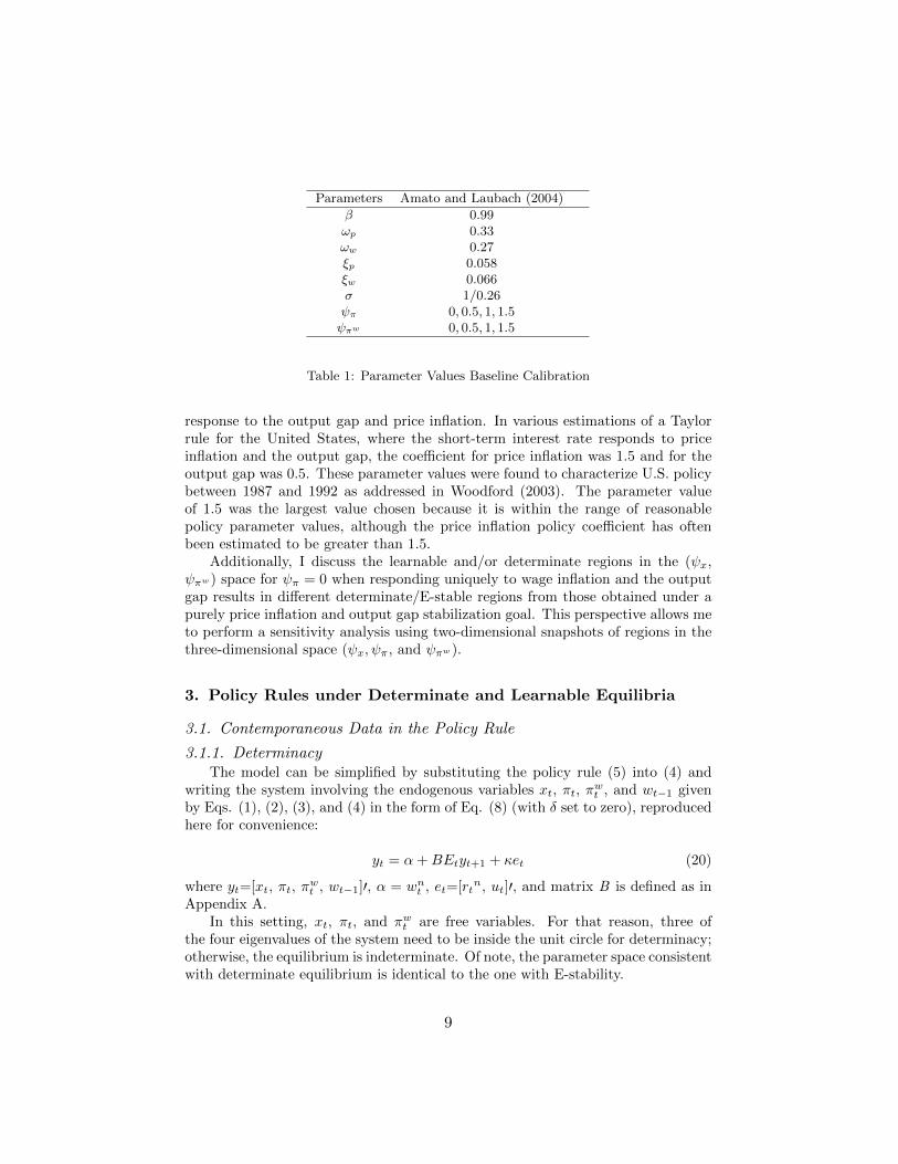
In most cases analytic results are not tractable and so I proceed numerically asin Galı (2008), Evans and McGough (2007), and Bullard and Mitra (2007). Themodel was calibrated with parameter values from Amato and Laubach (2004).9
They estimated impulse responses of wages and prices to a monetary policy shock.These parameters are considered the baseline calibration. The robustness of resultsare also verified under the alternative calibration from Giannoni and Woodford(2003).
In order to illustrates the learnable and/or determinate regions of the parameterspace for the Taylor rule specifications previously outlined, Figures 1–5 are drawnin (ψx, ψπ) space with all the other parameters set to their baseline values exceptfor ψπw = 0, 0.5, 1, and 1.5 and ψi = 0, 0.65, and 5. The wage inflation parametervalue of 0 corresponds to a rule where the interest rate is responding only to priceinflation and the output gap—the BM result. The values 0.5 and 1 correspond toa rule with a moderate to aggressive response to wage inflation in addition to the
9The authors extend the analysis of Rotemberg and Woodford (1997) by adding a realwage series to a VAR.
response to the output gap and price inflation. In various estimations of a Taylorrule for the United States, where the short-term interest rate responds to priceinflation and the output gap, the coefficient for price inflation was 1.5 and for theoutput gap was 0.5. These parameter values were found to characterize U.S. policybetween 1987 and 1992 as addressed in Woodford (2003). The parameter valueof 1.5 was the largest value chosen because it is within the range of reasonablepolicy parameter values, although the price inflation policy coefficient has oftenbeen estimated to be greater than 1.5.
Additionally, I discuss the learnable and/or determinate regions in the (ψx,ψπw) space for ψπ = 0 when responding uniquely to wage inflation and the outputgap results in different determinate/E-stable regions from those obtained under apurely price inflation and output gap stabilization goal. This perspective allows meto perform a sensitivity analysis using two-dimensional snapshots of regions in thethree-dimensional space (ψx, ψπ, and ψπw).
3. Policy Rules under Determinate and Learnable Equilibria
3.1. Contemporaneous Data in the Policy Rule
3.1.1. DeterminacyThe model can be simplified by substituting the policy rule (5) into (4) and
writing the system involving the endogenous variables xt, πt, πwt , and wt−1 given
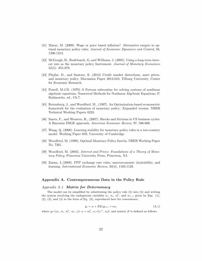
by Eqs. (1), (2), (3), and (4) in the form of Eq. (8) (with δ set to zero), reproducedhere for convenience:
yt = α+BEtyt+1 + κet (20)
where yt=[xt, πt, πwt , wt−1]′, α = wnt , et=[rt
n, ut]′, and matrix B is defined as inAppendix A.
In this setting, xt, πt, and πwt are free variables. For that reason, three ofthe four eigenvalues of the system need to be inside the unit circle for determinacy;otherwise, the equilibrium is indeterminate. Of note, the parameter space consistentwith determinate equilibrium is identical to the one with E-stability.
9
3.1.2. LearningI assume that yt is not available when the forecasts Etyt+1 are formed, and the
information set is represented by (1, yt−1, e′t).
10 The model is written as
yt = α+ BEtyt+1 + δyt−1 + κ et, (21)
where yt=[xt, πt, πwt , wt]′, α = wnt , et=[rt
n, ut]′, and matrices B, δ, and κ aredefined as in Appendix A.
The MSV solution takes the form of Eq. (9).11 Equation (9) for b is charac-terized by a matrix quadratic that could have multiple solutions. The determinateequilibrium corresponds to the case where there is a unique solution for b with all ofits eigenvalues inside the unit circle. This paper analyzes stability under adaptivelearning of REE that are asymptotically stationary. It is possible to analyze stabil-ity under adaptive learning of explosive solutions but here I focus on the solutionsthat are asymptotically stable. The solution to matrix b was obtained using the“trust-region-dogleg” method for systems of non-linear equations (for a detaileddescription see Powell, 1970).
E-stability of the MSV solution under learning is now considered. The PLMtakes the form of the MSV solution. The mapping from PLM to ALM takes theform of Eq. (15). To compute the E-stability conditions I use derivatives (17), (18),and (19), where the three matrices require real parts less than 1 for E-stability. If atleast one of the eigenvalues of the matrices has a real part greater than 1, then theequilibrium is E-unstable. After finding the MSV solution, E-stability conditionswere numerically evaluated. The results are discussed in the next subsections.
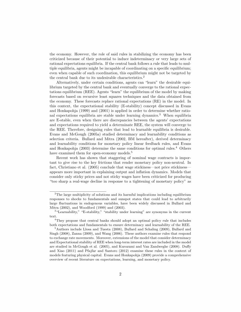
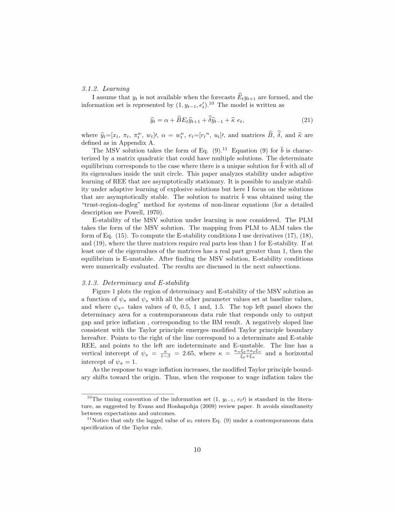
3.1.3. Determinacy and E-stabilityFigure 1 plots the region of determinacy and E-stability of the MSV solution as
a function of ψπ and ψx with all the other parameter values set at baseline values,and where ψπw takes values of 0, 0.5, 1 and, 1.5. The top left panel shows thedeterminacy area for a contemporaneous data rule that responds only to outputgap and price inflation , corresponding to the BM result. A negatively sloped lineconsistent with the Taylor principle emerges–modified Taylor principle boundaryhereafter. Points to the right of the line correspond to a determinate and E-stableREE, and points to the left are indeterminate and E-unstable. The line has avertical intercept of ψx = κ
1−β = 2.65, where κ =κwξp+κpξwξp+ξw
and a horizontal
intercept of ψπ = 1.As the response to wage inflation increases, the modified Taylor principle bound-
ary shifts toward the origin. Thus, when the response to wage inflation takes the
10The timing convention of the information set (1, yt−1, et′) is standard in the litera-ture, as suggested by Evans and Honkapohja (2009) review paper. It avoids simultaneitybetween expectations and outcomes.
11Notice that only the lagged value of wt enters Eq. (9) under a contemporaneous dataspecification of the Taylor rule.
10
Figure 1: Determinacy and learnability for a model with contemporaneous data in thepolicy rule. All parameters except for ψπ and ψx are set at baseline values.
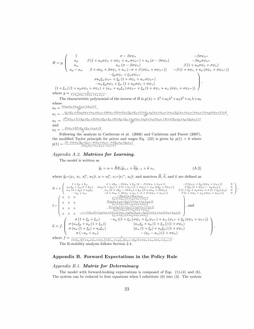
value of (ψπw = 0.50), the response to price inflation must also be 0.50 in order toinduce determinacy and E-stability. In fact, determinacy and E-stability under acontemporaneous data rule are governed by the following modified version of theTaylor principle for a combination of wages and prices:
ψπ + ψπw +(1− β)
κψx > 1. (22)
Eq. (22) is consistent with the numerical analysis and its derivation is discussed inAppendix A. This reformulated Taylor principle matches the determinacy conditionof Flaschel et al. (2008) and Flaschel and Franke (2009).12
In order to shed some light on the economic interpretation of this reformulatedTaylor principle, Eqs. (1) and (2) can be redefined using a particular weighted
average of wage and price inflation π =ξ−1p πt+ξ
−1w πwt
ξ−1p +ξ−1
w, as in Woodford (2003). Now
the Phillips curves reduce to:
π = κ(Yt − Y nt ) + βEtπt+1. (23)
The coefficient κ = σ−1+ωξ−1p +ξ−1
w, which is identical to κ, becomes smaller the greater
12I drew values of ψπ, ψπw , and ψx from a uniform distribution [0,10]. I recordedwhether the equilibrium was determinate and E-stable for values of ψπ + ψπw > 1. Irepeated this exercise 1 million times; in 100 percent of the cases when ψπ +ψπw > 1, theequilibrium was determinate and E-stable.
11
the degree of rigidity of either wages or prices. When only wages (prices) are sticky,Eq. (23) becomes a Phillips curve for wages (prices). Using the methodology inAscari and Ropele (2009), from Eq. (23) it can be observed that each percentagepoint of permanently higher weighted average of inflation leads to a long-run in-crease in the output gap of ((1− β)/κ) percentage points. Thus the left hand sideof Eq. (22) represents the long run increase in the nominal interest rates proposedby the policy rule (5) for each unit of permanent increase in the inflation rate. Inany case, the Phillips curve for wages is analogous to the Phillips curve for prices,therefore, when the Taylor principle is satisfied, a departure of the private sectorexpected inflation (price and/or wage) from RE value will increase the real interestrate. The increase in the real interest rate would reduce output through Eq. (4)leading to a reduction of inflation through Eqs. (1) and (2) or (23), under thetraditional demand channel.13
Wage stickiness has proven to be a key element that improves the empiricalfit of the model and explains the real effects of monetary policy. Incorporatingwage stickiness could potentially alter equilibrium determinacy (Ascari et al., 2011;Carlstrom and Fuerst, 2007; and Huang et al., 2009) and E-stability conditions. Iproceed by considering whether increasing the degree of wage stickiness, representedby decreasing ξw (going from 0.066, the value assigned in our baseline calibration,to 0.0042 in Giannoni and Woodford, 2003), affects equilibrium determinacy andE-stability. I find that a policy rule that responds to contemporaneous data hasanalogous implications for determinacy of REE and stability under learning, regard-less of the source of rigidity. As κ decreases (due to stickier prices or wages), themodified Taylor principle boundary pivots downward, finding its vertical interceptat ψx = κ
1−β , expanding the determinate and E-stability region.
3.2. Forward Expectations in the Policy Rule
3.2.1. DeterminacyThe model with forward-looking expectations is composed of Eqs. (1)-(4) and
(6) for ψi = 0. The system can be reduced to four equations when I substitute Eq.(6) into Eq. (4). The analysis follows Section 3.1.1, with matrix B defined as inAppendix B.
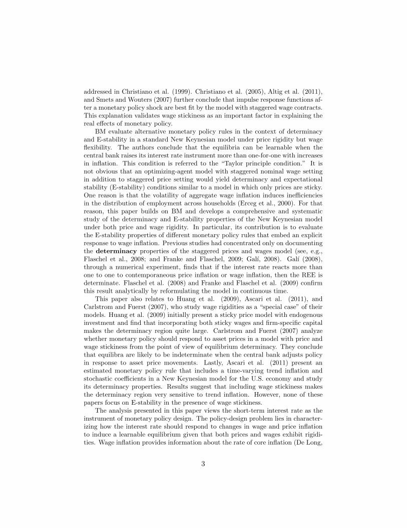
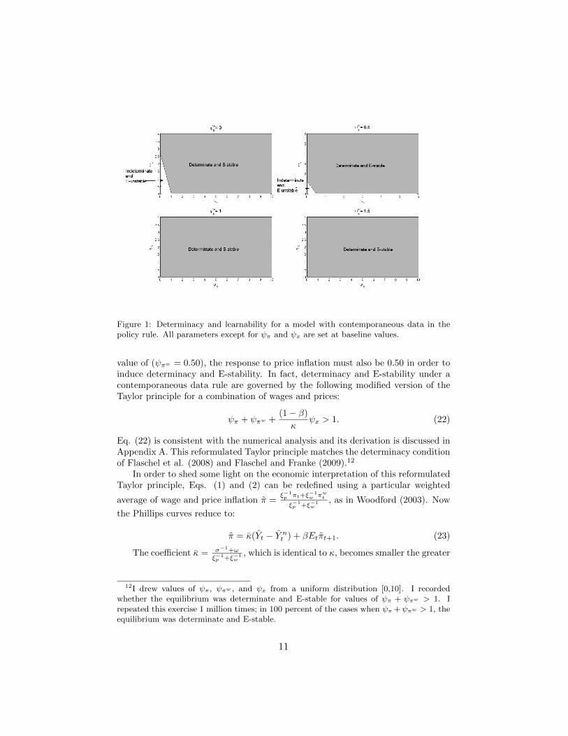
Fig. 2 presents the numerical results. When the central bank responds only toforward expectations of price inflation and the output gap in the policy rule (Case1) the determinate equilibrium occurs when ψπ > 1, consistent with the modified
13This paper also analyzes determinacy and E-stability conditions for a Taylor rule thatis responding to contemporaneous expectations in its policy feedback rule or nowcasting:it = ψπEtπt + ψπw Etπ
wt + ψxEtxt. Policymakers condition their policy instruments on
expected values of current wage and price inflation, and the output gap. Determinacyand E-stability conditions are identical to the case with contemporaneous data in thepolicy feedback rule under the assumption present in this paper regarding observabilityof exogenous processes. I follow the conditions for determinacy and E-stability outlinedin Evans and McGough (2005a).
12
Taylor principle condition, and ψx < 0.52. Under the benchmark calibration, asthe response to price (wage) inflation increases, the response to the output gapshould gradually decrease concurrently in order to yield a determinate REE–e.g.,when ψπ = 15 (ψπw = 15), ψx < 0.38 (ψx < 0.27) ensures determinacy.
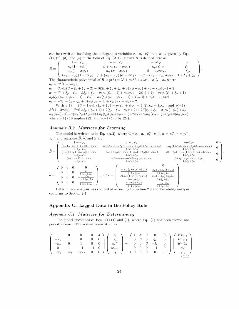
The numerical analysis matches the following boundary that divides the pa-rameter space into determinate and indeterminate regions
where a1 = (2ξp + 2ξw + 2κpσ)(1 + β) + 4(β + 1)2.This boundary is similar to Eq. (40) from BM and it has also been documented
by Galı (2008) and Bernanke and Woodford (1997) for rules that respond only toexpected future price inflation and expected future output gap under price stick-iness.14 It posits an upper bound constraint on response coefficients which showsup in forward-looking rules that guarantees equilibrium determinacy.
In the current analysis, determinacy of equilibrium under forward looking rulesrequires that (i) the central bank should respond neither too strongly nor too weaklyto price and/or wage inflation, and not too strongly to the output gap. Therefore,the Taylor principle condition is insufficient to guarantee determinacy; adjustinginterest rates strongly in response to changes in expected inflation or the expectedoutput gap can lead to equilibrium fluctuations attributed to self-fulfilling expec-tations. (ii) The central bank should also be mindful of the degrees of price andwage stickiness prevailing in the economy when conducting its policy design. Thedeterminacy area is now sensitive to the degree of price and wage rigidity throughits effects on κw and κπ, along with the type of inflation (π or πw) that the centralbank chooses to target.
If κp = κw, then determinacy would not be affected by whether the central bankdecides to respond to expected future π or πw in the Taylor rule. In practice theseparameters are not necessarily equal. For example, the benchmark values usedherein are κp = 0.0191 and κw = 0.0350. Even when the quantitative differencesare not large for the calibration currently used, the results highlight the relativeroles of price and wage stickiness for policy feedback rules that respond to expectedfuture variables.15 If one type of stickiness was more important in practice thiswould lead to even stronger implications for policy. When, for instance, wagestickiness is higher, so that κw < κp, a policy that responds to wage inflationhas a larger determinacy region. Responding to wage inflation pivots upward thedeterminacy boundary (24) and it ensures that the equilibrium is determinate evenfor high values of ψπw . Thus, having a central bank that tries to demonstratethe seriousness with which it takes its inflation target is not problematic becauseresponding particularly strongly to a type of inflation forecast is not conducive toindeterminacy.
14Details on its derivation are included in Appendix B.15This is also the case for lagged data rules, discussed later in the text.
13
Under Eq. (5), wage and price inflation have symmetric contemporaneous ef-fects on the output gap through the interest rate. However, when the central bankresponds to expected price and wage inflation as in Eq. (6), expected price infla-tion enters directly through the interest rate and through the IS equation, whileexpected wage inflation affects output only through the interest rate. Therefore,it is not surprising that the forward looking case postulates different underlyingimplications for determinacy from the contemporaneous data case.
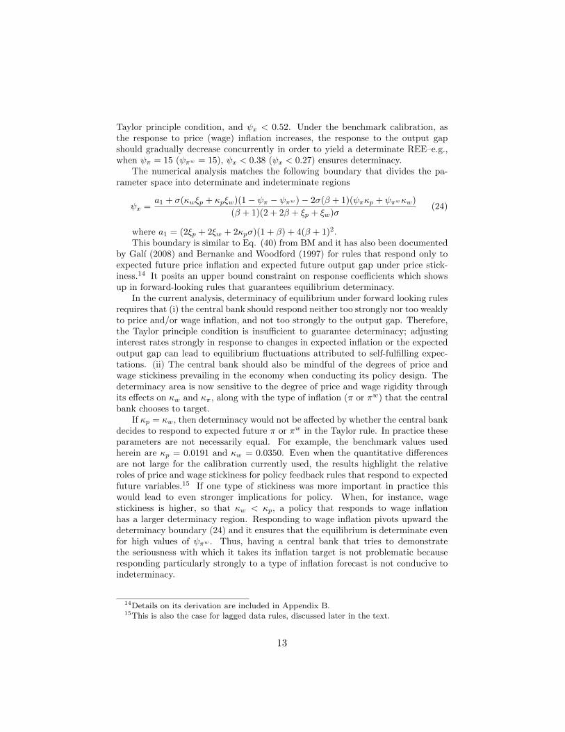
3.2.2. E-stabilityThe E-stability conditions for rules with forward-looking expectations in the
policy rule are akin to the analysis in Section 3.1.2. Matrices B, δ, and κ aredefined in Appendix B.16
Figure 2: Determinacy and learnability for a model with forward expectations in thepolicy rule. All parameters except for ψπ and ψx are set at baseline values.
Fig. 2 plots the E-stable region of the MSV solution. The modified Taylorprinciple given by Eq. (22) is sufficient to guarantee E-stability of REE. The MSVsolution is learnable even when found in the indeterminate region of the parameterspace; the converse, however, is not true.
3.3. Lagged Data in the Policy Rule
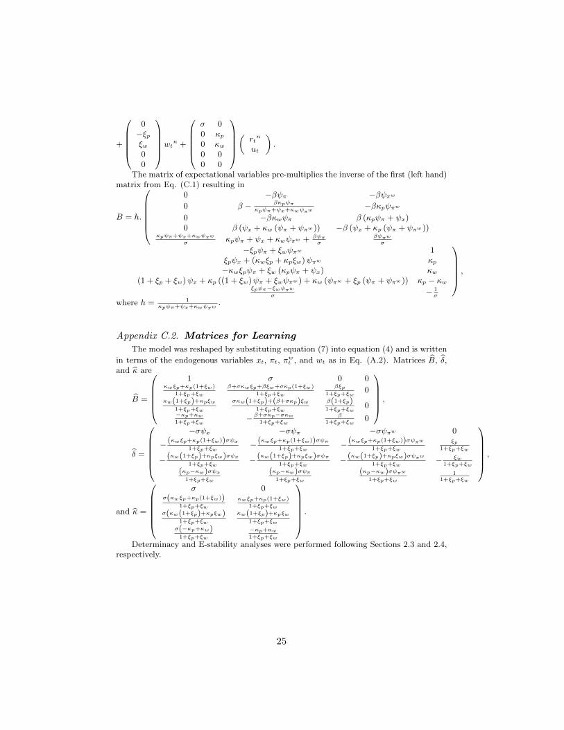
3.3.1. DeterminacyThe model encompasses Eqs. (1)-(4) and (7), where Eq. (7) for ψi = 0 has
been moved one period forward and is represented in Appendix C. The matrix ofexpectational variables pre-multiplies the inverse of the first (left hand) matrix from
16Only the lagged value of wt enters Eq. (10) under the forward-looking policy function.
14
Eq. (C.1) resulting in Matrix B, which is the appropriate matrix for determinacyanalysis. Determinacy analysis follows Section 3.1.1.
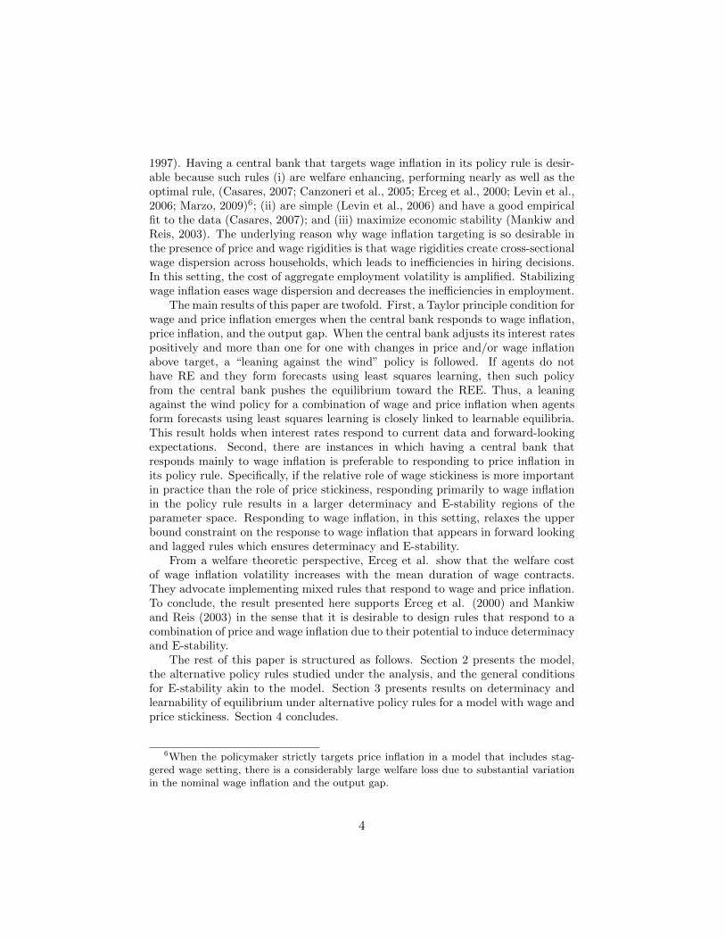
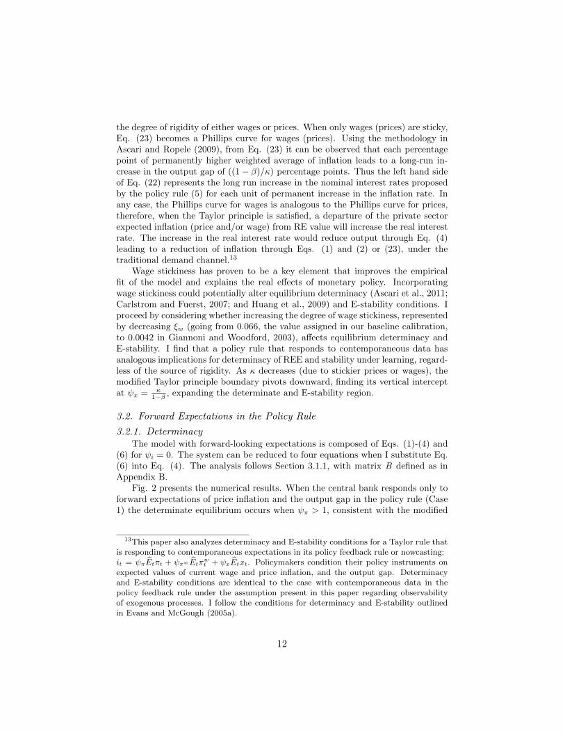
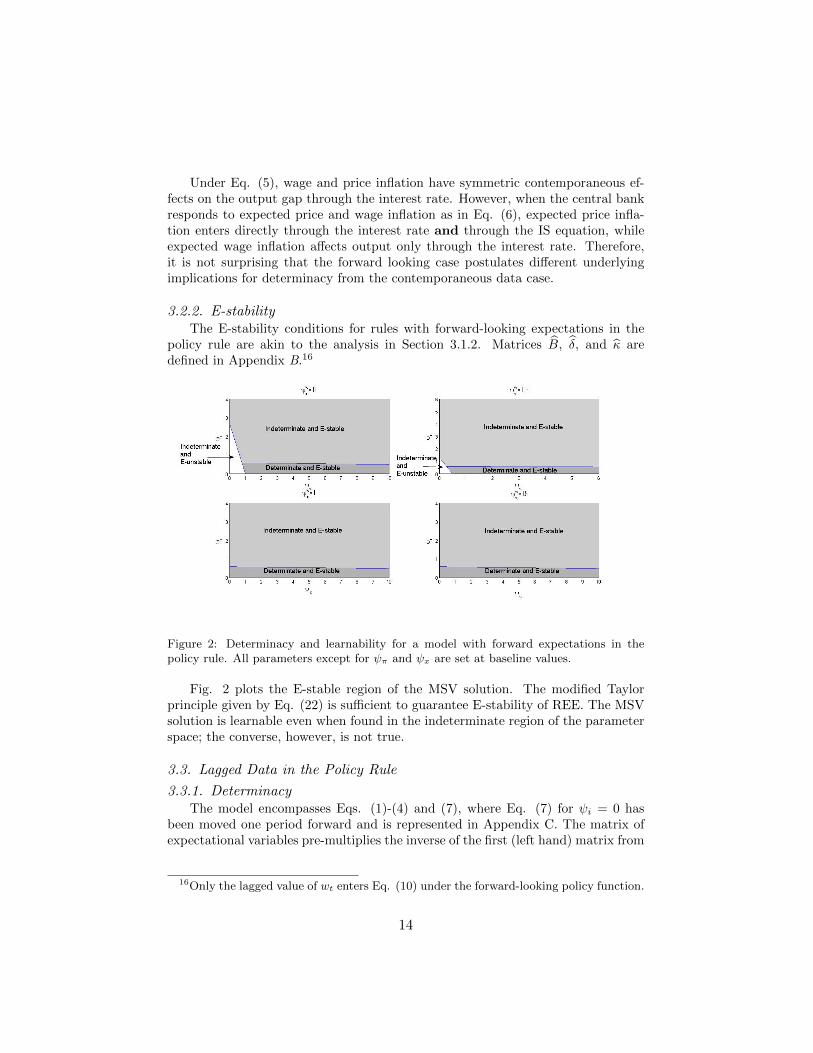
3.3.2. DeterminacyFig. 3 plots the determinacy region. When the central bank responds to lagged
price inflation and lagged output gap the modified Taylor principle boundary andthe determinacy boundary (24) appear. Two determinacy regions emerge: Region1 for values of ψπ > 1 and a modest value for ψx (less than 0.52), analogous tothe determinacy region under forward expectations in the policy rule, thereforesensitive to changes in wage stickiness.
Region 2 for values to the left of the negatively sloped line, where ψπ is at most0.8 and 0.52 < ψx < 2.65. Determinacy in this setting posits a trade-off between(i) a relatively large response to lagged inflation (greater than 1) and a relativelysmall response to lagged output gap or (ii) a relatively large response to laggedoutput gap and a relatively small response to lagged price inflation. Therefore, withlagged data in the policy rule the Taylor principle condition is neither necessarynor sufficient to guarantee uniqueness of equilibrium. As the combined response toinflation increases and achieves a value greater than 1, the only determinate areathat prevails is Region 1.
3.3.3. E-stabilityThe model was reshaped as in Section 3.1.2. See Appendix C for matrices B,
δ, and κ. E-stability analysis follows Section 3.1.2.
Figure 3: Determinacy and learnability for a model with lagged data in the policy rule.All parameters except for ψπ and ψx are set at baseline values.
15
Fig. 3 shows the E-stable regions of the MSV solutions. The E-stable region ofthe parameter space is analogous to determinacy Region 1. The upper-left panelis qualitatively close to BM, but the position of the line separating the explosiveregion and the determinate and E-stable region is now affected by the degree ofwage stickiness.
3.4. Policy Inertia
In the policy inertia case, the systems of equations are given by (1)-(4), and(6) for the system with forecast data, and Eq. (7) for the system with lagged data,and policy inertia in the monetary policy rule. The analysis of determinacy and E-stability of the MSV solution is standard and follows Sections 2.3 and 2.4.17 As inBullard and Mitra (2007), analytical solutions were not obtained for the E-stabilityconditions of stationary MSV solutions, however the results are discussed using thebaseline calibration values of Amato and Laubach (2004).
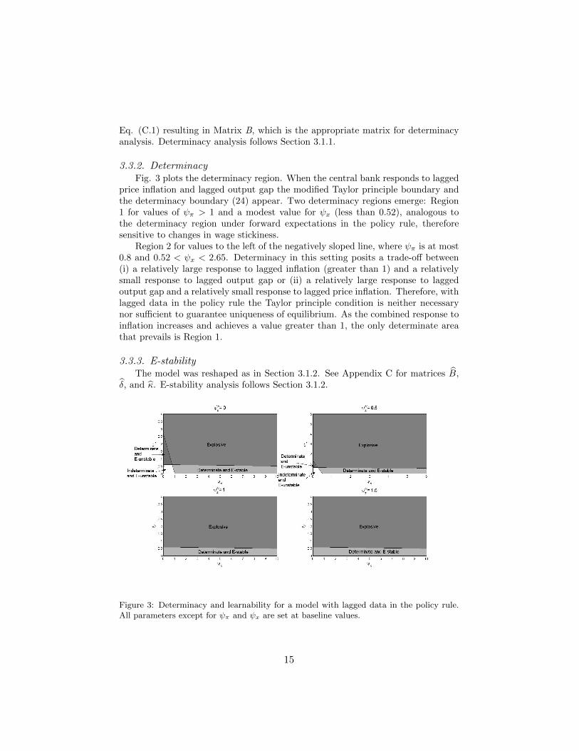
Figure 4: Determinacy and learnability for a model with policy inertia in the forwardlooking policy rule. Parameter ψi takes on values of 0.65, 0.65 and 5, and ψπw values of0, 0.5, and 0. All other parameters except for ψπ and ψx are set at baseline values.
Under the policy rule that responds to forward expectations and policy inertia,the results, plotted in Fig. 4, compare quantitatively to the graphs without policyinertia, Fig. 3, as follows: when ψi = 0.65 without any response to wage inflation(first panel of Fig. 4 from left to right), the horizontal line that divides the pa-rameter space shifts upward and now has an intercept of roughly 0.90 (before itwas 0.52); the determinacy and learnable area is now more prominent. The secondpanel on Fig. 4 shows a further increase in the desirable area as the response towage inflation increases (ψπw = 0.50). Moreover, a strong response to policy iner-tia ψi = 5 yields a an even larger determinate and E-stable region (third panel ofFig. 4); however, the same desirable region prevails for higher values of ψπw (i.e.
17The matrices obtained when performing the determinacy and E-stability of stationaryMSV solution analyses are available upon request.
16
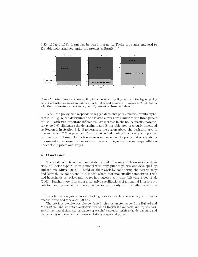
0.50, 1.00 and 1.50). It can also be noted that active Taylor-type rules may lead toE-stable indeterminacy under the present calibration.18
Figure 5: Determinacy and learnability for a model with policy inertia in the lagged policyrule. Parameter ψi takes on values of 0.65, 0.65, and 5, and ψπw values of 0, 0.5 and 0.All other parameters except for ψπ and ψx are set at baseline values.
When the policy rule responds to lagged data and policy inertia, results repre-sented in Fig. 5, the determinate and E-stable areas are similar to the three panelsof Fig. 4 with two important differences: An increase in the policy inertial parame-ter ψi to 0.65 eliminates the determinate and E-unstable area previously describedas Region 2 in Section 3.3. Furthermore, the region above the desirable area isnow explosive.19 The prospect of rules that include policy inertia of yielding a de-terminate equilibrium that is learnable is enhanced as the policymaker adjusts itsinstrument in response to changes in—forecasts or lagged—price and wage inflationunder sticky prices and wages.
4. Conclusion
The study of determinacy and stability under learning with various specifica-tions of Taylor type-rules in a model with only price rigidities was developed byBullard and Mitra (2002). I build on their work by considering the determinacyand learnability conditions in a model where monopolistically competitive firmsand households set prices and wages in staggered contracts following Erceg et al.(2000). Furthermore, I consider alternative specifications of a nominal interest raterule followed by the central bank that responds not only to price inflation and the
18For a further analysis on forward looking rules and stable indeterminacy with inertiarefer to Evans and McGough (2005c).
19The previous exercise was also conducted using parameter values from Bullard andMitra (2007) and we obtain analogous results; (i) Region 2 disappears and (ii) the hori-zontal line that divides the parameter space shifts upward, making the determinate andlearnable region larger in the presence of sticky wages and prices.
17
output gap, but also to wage inflation. The main result is twofold. First, whenthe central bank responds to wage and price inflation and the output gap, a modi-fied Taylor principle for wage and price inflation arises: The nominal interest rateshould be adjusted more than one for one with changes in (wage and/or price) infla-tion. This Taylor principle is closely linked with stability under learning dynamicswhen the central bank responds to current data and forward-looking expectations.Furthermore, when the central bank adjusts the interest rate in response to laggeddata, the policy instrument must (i) respond moderately to changes in the outputgap and wage/price inflation and (ii) meet the modified Taylor principle conditionin order to yield stability under learning dynamics.
Second, results show that sticky wages and sticky prices have an impact on thedeterminacy and E-stability areas of the parameter space. If one type of stickinesswas more important in practice this would lead to strong implications for policydesign. When, for instance, wage stickiness plays a more significant role that pricestickiness, it is preferable to target wage inflation than price inflation because suchpolicy yields a larger determinacy and E-stable region. In particular, it relaxesthe upper bound constraint on the central bank’s response to wage inflation nec-essary to ensure determinacy and E-stability. Thus, having a central bank thatattempts to demonstrate the seriousness with which it takes its inflation target isno longer an issue, because responding extremely vigorously to wage inflation isnot conducive to indeterminacy or instability under learning dynamics. This resultsupports Woodford (2003) and Erceg et al. (2000) in the sense that the degree ofwage and/or price stickiness affects the monetary policy stabilization goals. Theyfind that in the extreme case of only sticky wages, optimal policy entails completestabilization of wages. In practice they advocate seeking to stabilize an appropriateweighted average of wage and price inflation. Herein, results suggest that a centralbanker concerned with avoiding indeterminacy and/or instability under learningshould consider responding to wage inflation in addition to price inflation.
Acknowledgements: I especially thank Bill Branch for his advice and helpin many aspects of this project. I also thank Michelle Garfinkel, Judy Ahlers,James Bullard, Pavel Kapinos, and anonymous referees for important input intothis paper. I also want to thank the Department of Economics and School of SocialSciences at the University of California, Irvine for financial support.
18
5. References
[1] Amato, J., and Laubach, T. (2004). Implications of habit formation for optimalmonetary policy.Journal of Monetary Economics, 51, 305-325.
[2] Ascari, G., and Ropele, T. (2009). Trend Inflation, Taylor Principle and Inde-terminacy. Bank of Italy Working Paper No. 708.
[3] Ascari,G., Branzoli, N. and E. Castelnuovo (2011). Trend Inflation, Wage In-dexation, and Determinacy in the U.S. mimeo. University of Pavia.
[4] Altig, D., Lawrence, C., Eichenbaum, M., and Linde, J. (2011). Firm-specificcapital, nominal rigidities and the business cycle. Review of Economic Dynam-ics, 14(2), 225-247.
[5] Bernanke, B., and Woodford, M. (1997). Inflation Forecasts and MonetaryPolicy. Journal of Money, Credit and Banking, 29(4), 653-684.
[6] Best, G. and Kapinos, P. (2015). In What Sense Is Monetary Policy Forward-Looking? mimeo. California State University, Fullerton.
[7] Brainard, W. (1967). Uncertainty and the effectiveness of policy. AmericanEconomic Review 57, 411-425.
[8] Bullard, J., and Mitra, K. (2002). Learning about monetary policy rules. Jour-nal of Monetary Economics, 49, 1105-1129.
[9] Bullard, J., and Mitra K. (2007). Determinacy, learnability, and monetarypolicy inertia. Journal of Money, Credit and Banking, 39, (5) 1177-1212.
[10] Bullard, J., and Schaling, E. (2009). Monetary policy, determinacy, and learn-ability in a two-block world economy. Journal of Money, Credit and Banking,41(8), 1585-1612.
[11] Bullard, J., and Singh, A. (2008). Worldwide macroeconomic stability andmonetary policy rules. Journal of Monetary Economics, 55(Supplement), S34-S47.
[12] Canzoneri, M., Cumby, R., and Diba, B. (2005). Price and Wage Inflation Tar-geting: Variations on a Theme by Erceg, Henderson and Levin. in Jon Faust,Athanasios Orphanides and David Reifschneider, eds., Models and MonetaryPolicy: Research in the Tradition of Dale Henderson, Richard Porter, and Pe-ter Tinsley, Board of Governors of the Federal Reserve System: WashingtonDC, 2005.
[13] Carlstrom C., Fuerst T. and Ghironi, F. (2006). Does it matter (for equilibriumdeterminacy) what price index the central bank targets? Journal of EconomicTheory, 128,1, 214-231.
19
[14] Carlstrom, C., and Fuerst T. (2007). Asset prices, nominal rigidities and mon-etary policy. Review of Economic Dynamics, 10, 256-275.
[15] Casares, M. (2007) Monetary policy rules in a New Keynesian euro area model.Journal of Money, Credit and Banking, 39, 4, 875-900.
[16] Christiano, L., Eichenbaum, M., and Evans, C. (1999). Monetary PolicyShocks: What Have We Learned and to What End? In Handbook of Macroe-conomics 1A.
[17] Christiano, L., Eichenbaum, M., and Evans, C. (2005). Nominal Rigiditiesand the Dynamic effects of a Shock to Monetary Policy. Journal of PoliticalEconomy 113, 1-45.
[18] Clarida, R., Gali, J., and Gertler, M. (1998). Monetary Policy Rules in Prac-tice: Some International Evidence. European Economic Review 42, 1033-1067.
[19] Cukierman, A. (1989). Why does the Fed smooth interest rates? In MonetaryPolicy on the 75th Anniversary of the Federal Reserve System, Belgonia M(ed.). Kluwer Academica Press: Boston, MA.
[20] De Long, B. (1997). America’s Only Peacetime Inflation: The 1970s. In Romer,C. and Romer, D. Eds., Reducing Inflation, University of Chicago Press,CHicago.
[21] Dennis, R. (2006). The Policy Preferences of the US Federal Reserve. Journalof Applied Econometrics 21, 55-77.
[22] Duffy, J. and Xiao, W. (2011). Investment and monetary policy: learning anddeterminacy of equilibrium. Journal of Money, Credit and Banking, 43(5),959-992.
[23] Erceg, C., Henderson D., and Levin A., (2000). Optimal monetary policy withstaggered wage and price contracts. Journal of Monetary Economics, 46, 281-313.
[24] Evans, G., and Honkapohja, S. (1999). Learning dynamics. Handbook ofMacroeconomics, 1(A), 449-542.
[25] Evans, G., and Honkapohja, S. (2001). Learning and Expectations in Macroe-conomics Monetary. Princeton University Press, Princeton, NJ..
[26] Evans, G., and Honkapohja, S. (2003). Adaptive Learning and Monetary PolicyDesign. Journal of Money, Credit and Banking 35(6), 1045-1073.
[27] Evans, G., and Honkapohja, S. (2009). Expectations, learning and monetarypolicy: an overview of recent research. In Central Banking Analysis, and Eco-nomic Policies Book Series, in Klaus Schmidt-Hebbel, Carl E. Walsh, and Nor-man Loayza (Series Editors). Monetary Policy under Uncertainty and Learn-ing, Ed. 1, Vol. 13, Ch. 2, pp. 27-76.
20
[28] Evans, G., and McGough, B. (2005a). Monetary policy, indeterminacy andlearning. Journal of Economic Dynamics and Control 29, 1809-1840.
[29] Evans, G., and McGough, B. (2005b). Stable sunspot solutions in models withpredetermined variables. Journal of Economic Dynamics and Control 29, 601- 625.
[30] Evans, G. and McGough, B. (2005c). Monetary policy and stable indetermi-nacy.Economics Letters 87, 1-7.
[31] Evans, G., and McGough, B. (2007). Optimal constrained interest-rate rules.Journal of Money, Credit, and Banking 39(6), 1335-1356.
[32] Flaschel, P., Franke, R., and Proano, C. (2008). On equilibrium determinacyin New Keynesian models with staggered wage and price setting. B.E. Journalof Macroeconomics, 8(1).
[33] Franke, R., and Flaschel, P. (2008). A Proof of Determinacy in the New-Keynesian Sticky Wages and Prices Model. Economics Working Papers2008,14, Christian-Albrechts-University of Kiel, Department of Economics.
[34] Galı, J. (2008). Monetary policy, inflation and the business cycle: An intro-duction to the New Keynesian Framework. Princeton University Press.
[35] Giannoni, M., and Woodford, M. (2003). Optimal interest-rate rules: I. Gen-eral theory. NBER Working Papers 9419.
[36] Huang, K., Meng, Q., and Xue, J. (2009). Is forward-looking inflation tar-geting destabilizing? The role of policy’s response to current output underendogenous investment. Journal of Economic Dynamics and Control, 33(2),409-430.
[37] Kurozumi, T., and Van Zandweghe, W. (2008) Investment, interest rate policy,and equilibrium stability. Journal of Economic Dynamics and Control, 32(5),1489-516.
[38] Levin, A., Onatski, A., Williams, J., and Williams N. (2006). Monetary pol-icy under uncertainty in micro-founded macroeconometric models. in NBERMacroeconomics Annual 2005, Volume 20, MIT Press.
[39] Llosa, L., and Tuesta V. (2008). Determinacy and learnability of monetarypolicy rules in small open economies. Journal of Money, Credit and Banking,40(5), 1033-1063.
[40] Mankiw, N.G., and Reis, R. (2003). What measure of inflation should a centralbank target? Journal of the European Economic Association, 1(5): 1058-1086.
21
[41] Marzo, M. (2009). Wage or price based inflation? Alternative targets in op-timal monetary policy rules. Journal of Economic Dynamics and Control, 33,1296-1313.
[42] McGough, B., Rudebusch, G, and Williams, J. (2005). Using a long-term inter-est rate as the monetary policy Instrument. Journal of Monetary Economics52(5): 855-879.
[43] Pfajfar, D., and Santoro, E. (2012) Credit market distortions, asset prices,and monetary policy. Discussion Paper 2012-010, Tilburg University, Centerfor Economic Research.
[44] Powell, M.J.D. (1970) A Fortran subroutine for solving systems of nonlinearalgebraic equations, Numerical Methods for Nonlinear Algebraic Equations, P.Rabinowitz, ed., Ch.7.
[45] Rotemberg, J., and Woodford, M., (1997). An Optimization-based econometricframework for the evaluation of monetary policy: Expanded version. NBERTechnical Working Papers 0233.
[46] Smets, F., and Wouters, R., (2007). Shocks and frictions in US business cycles:A Bayesian DSGE approach. American Economic Review, 97, 586-606.
[47] Wang, Q. (2006). Learning stability for monetary policy rules in a two-countrymodel. Working Paper 659, University of Cambridge
[48] Woodford, M. (1999). Optimal Monetary Policy Inertia. NBER Working PaperNo. 7261.
[49] Woodford, M. (2003). Interest and Prices: Foundations of a Theory of Mone-tary Policy. Princeton University Press, Princeton, NJ.
Following the analysis in Carlstrom et al. (2006) and Carlstrom and Fuerst (2007),the modified Taylor principle for prices and wages Eq. (22) is given by p(1) < 0 where
Appendix B. Forward Expectations in the Policy Rule
Appendix B.1. Matrix for Determinacy
The model with forward-looking expectations is composed of Eqs. (1)-(4) and (6).The system can be reduced to four equations when I substitute (6) into (4). The system
23
can be rewritten involving the endogenous variables xt, πt, πwt , and wt−1 given by Eqs.
(1), (2), (3), and (4) in the form of Eq. (A.1). Matrix B is defined here as