A new method to analyse impact-echo signals

Otto-Graf-Journal Vol. 12, 2001 81

A NEW METHOD TO ANALYSE IMPACT-ECHO SIGNALS

NEUE METHODE ZUR ANALYSE VON IMPACT-ECHO SIGNALEN

UNE NOUVELLE METHODE D’ANALYSE DES SIGNAUX IMPACT-

ECHO

Hans-Jürgen Ruck, Ralf Beutel

SUMMARY

The impact-echo method is a young diagnose for controlling the quality of

a construction. In this method, a stress pulse is introduced into an object by

mechanical impact on its surface, and this pulse undergoes multiple reflections

(echoes) between opposite faces of the object. To determine the frequency of the

detected signal usually the Fourier transform is used. In this article we apply the

new analysis tool, the wavelet transform, to the echo signal. In an example these

two types of signal analyses tools are compared on the basis of measurements

on a stairs like specimen.

ZUSAMMENFASSUNG

Die Impakt-Echo Methode gilt als noch recht junges Instrument in der

Bauwerksdiagnostik. Aussagen über den Signalinhalt der dabei erzeugten

Ultraschallsignale werden bisher nur über die Fourier-Transformation

gewonnen. Eine neue bzw. zusätzliche Auswertungsmethode beschreibt die

Wavelet-Transformation. Anhand zweier Messungen an einem stufenförmigen

Probekörper wurden einmal exemplarisch die beiden Auswertungsarten

gegenübergestellt, um die Aussagefähigkeit solcher Signale zu erhöhen.

RESUME

Dans le diagnostic du bâtiment, la méthode impact-echo est considérée

comme un instrument encore assez jeune. L’évaluation des signaux

ultrasoniques ne se fait jusqu'à présent que par transformation Fourier. La

transformation ondelette constitue une nouvelle méthode d'évaluation. Afin

d’améliorer l'évaluation de tels signaux, les deux méthodes ont été comparées de

façon exemplaire sur la base de mesures effectuées sur un échantillon en forme

d’escalier.

H.-J. RUCK, R. BEUTEL

82

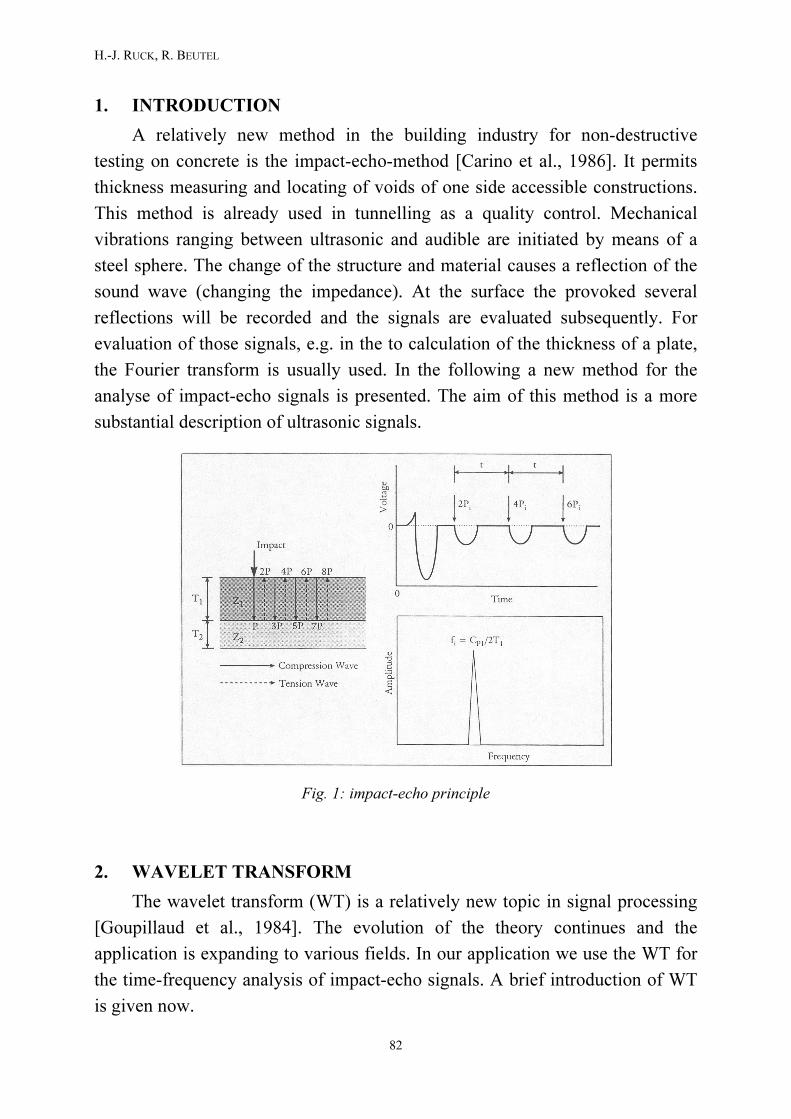
1. INTRODUCTION

A relatively new method in the building industry for non-destructive

testing on concrete is the impact-echo-method [Carino et al., 1986]. It permits

thickness measuring and locating of voids of one side accessible constructions.

This method is already used in tunnelling as a quality control. Mechanical

vibrations ranging between ultrasonic and audible are initiated by means of a

steel sphere. The change of the structure and material causes a reflection of the

sound wave (changing the impedance). At the surface the provoked several

reflections will be recorded and the signals are evaluated subsequently. For

evaluation of those signals, e.g. in the to calculation of the thickness of a plate,

the Fourier transform is usually used. In the following a new method for the

analyse of impact-echo signals is presented. The aim of this method is a more

substantial description of ultrasonic signals.

Fig. 1: impact-echo principle

2. WAVELET TRANSFORM

The wavelet transform (WT) is a relatively new topic in signal processing

[Goupillaud et al., 1984]. The evolution of the theory continues and the

application is expanding to various fields. In our application we use the WT for

the time-frequency analysis of impact-echo signals. A brief introduction of WT

is given now.

A new method to analyse impact-echo signals

Otto-Graf-Journal Vol. 12, 2001 83

The usual analysis tool for impact-echo signals is the Fourier transform

(FT). The FT and its inverse are defined as follows:

( ) ∫ −= dttitfF )exp()( ωω (1)

( ) ∫ −= dttitftf )exp()(2

1ω

π

(2)

where F(ω) is the Fourier transform and f(t) is the signal. In these equations

we multiplying the original signal with a complex expression which has sines

and cosines of frequency f and integrate this product. If the result of this

integration is a large value, then the signal f(t) has a dominant spectral

component at frequency f.

0,00 0,02 0,04 0,06 0,08

-10

-5

0

5

10

Amplitude

Zeit [s]

0 200 400 600 800 10000,0

0,5

1,0

1,5

2,0

2,5

3,0

3,5

Amplitude

Frequenz [Hz]Time [s] Frequency [Hz]

Fig.2: The signal 1 and the Fourier transform.

The integration is from minus infinity to plus infinity over time, so the

determination is impossible where in time the component with frequency f

appears. Therefore the FT is ideal for the analysis of stationary signals, whose

statistical properties do not change with time.

To analyse non-stationary or transient signals, another method that

transforms a signal into a joint time-frequency domain is necessary. Gabor

originated the windowed Fourier transform (WFT) as an extension to the

classical FT [Gabor, 1946]. Now f(t) is windowed by a window function g(τ-t)

which is shifted in time by changing τ over the whole signal. The WFT of f(t) is

defined as

( ) ( ) τωττω dtitgftF )exp(),( −−= ∫∞

∞−

(3)

H.-J. RUCK, R. BEUTEL

84

With the window function one cut out a part of the signal at a particular

time range and multiplying this range with the complex expression. The

integration of this product describes the dominance of the frequency f at the

time t. The problem with the WFT has to do with the steady width of the

window function. A short window width results in a good resolution in time, a

wide width in a good resolution in frequency. This is a consequence of the

uncertainty principle. If dt is the transform resolution in the time domain and dω

is the transform resolution in the frequency domain, the uncertainty principle

can be written as

2

1=∆∆ ωt . The WFT results in an intensity-graph where the x-axis

represents the time, the y-axis the frequency and the amplitude will be pictured

by several colours.

Fre

qu

ency

[H

z]

Time [ms]

Fig. 3: The WFT from the signal in picture 1. One can see the different frequencies at

different times. Light colours mean high amplitudes.

A new method to analyse impact-echo signals

Otto-Graf-Journal Vol. 12, 2001 85

A further extension of the WFT is the wavelet transform (WT) defined by

∫∞

∞−

−Ψ= dt

a

bttf

abaf )(

1),( (4)

with the shift parameter b, determines the position of the window in time

and thus defines which part of the signal f(t) is being analysed and the scale

variable a [Kaiser, 1994, Polkar, 1999]. In this investigation the relation

between the scale variable a controlling dilatation and the frequency is ω=ω0/a,

where ω0 is a positive constant. The wavelet function ψ(t) differs from the

sinusoidal function.

ψ(t) may be considered as a window function both in time and frequency

domain. The size of the time window is controlled by the translation, while the

length of the frequency band is controlled by the dilation. This property of the

WT is called multiresolution. A short window width correlates with a small

scale parameter results in a good resolution in time, a wide width in a good

resolution in frequency.

-0,15

-0,10

-0,05

0,00

0,05

0,10

0,15

0,20

0,25

Amplitude

Zeitachse

-0,4

-0,2

0,0

0,2

0,4

0,6

Amplitude

ZeitachseTime-axis Time-axis

Fig. 4: Two examples of wavelet functions. The Mexican Hat wavelet is placed on the left

side, the Morlet wavelet on the right side.

In practice one hold down the scale factor a and vary the shift parameter b.

The result shows the dominance of this frequency at every time. By changing

the scale factor and repeated scanning by altering b one get a 3-D plot of the

signal. The usually presentment is an intensity graph, where the x-axis

represents the time, the y-axis the scale and the intensities of the transform at

points in the a-b plane representing by a colour plate.

H.-J. RUCK, R. BEUTEL

86

Skal

ieru

ng

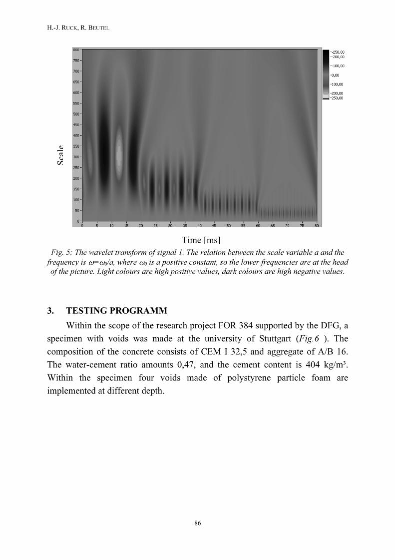
Zeit [ms] Fig. 5: The wavelet transform of signal 1. The relation between the scale variable a and the

frequency is ω=ω0/a, where ω0 is a positive constant, so the lower frequencies are at the head

of the picture. Light colours are high positive values, dark colours are high negative values.

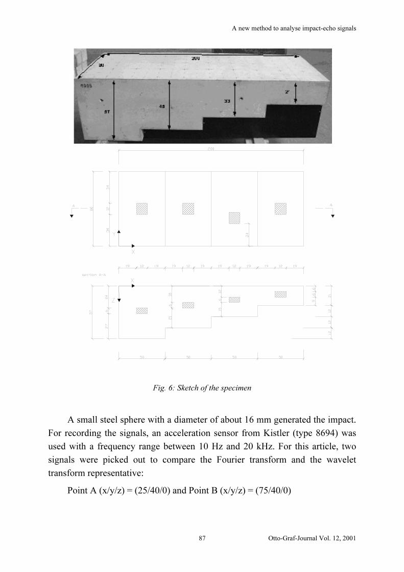
3. TESTING PROGRAMM

Within the scope of the research project FOR 384 supported by the DFG, a

specimen with voids was made at the university of Stuttgart (Fig.6 ). The

composition of the concrete consists of CEM I 32,5 and aggregate of A/B 16.

The water-cement ratio amounts 0,47, and the cement content is 404 kg/m³.

Within the specimen four voids made of polystyrene particle foam are

implemented at different depth.

Time [ms]

Scale

A new method to analyse impact-echo signals

Otto-Graf-Journal Vol. 12, 2001 87

Fig. 6: Sketch of the specimen

A small steel sphere with a diameter of about 16 mm generated the impact.

For recording the signals, an acceleration sensor from Kistler (type 8694) was

used with a frequency range between 10 Hz and 20 kHz. For this article, two

signals were picked out to compare the Fourier transform and the wavelet

transform representative:

Point A (x/y/z) = (25/40/0) and Point B (x/y/z) = (75/40/0)

H.-J. RUCK, R. BEUTEL

88

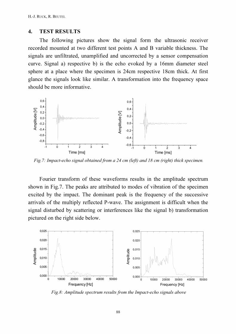
4. TEST RESULTS

The following pictures show the signal form the ultrasonic receiver

recorded mounted at two different test points A and B variable thickness. The

signals are unfiltrated, unamplified and uncorrected by a sensor compensation

curve. Signal a) respective b) is the echo evoked by a 16mm diameter steel

sphere at a place where the specimen is 24cm respective 18cm thick. At first

glance the signals look like similar. A transformation into the frequency space

should be more informative.

-1 0 1 2 3 4

-0,8

-0,6

-0,4

-0,2

0,0

0,2

0,4

0,6

Am

plit

ud

e [V

]

Time [ms]

-1 0 1 2 3 4-0,6

-0,4

-0,2

0,0

0,2

0,4

0,6

Time [ms]

Am

plitu

de [V

]

Fig.7: Impact-echo signal obtained from a 24 cm (left) and 18 cm (right) thick specimen.

Fourier transform of these waveforms results in the amplitude spectrum

shown in Fig.7. The peaks are attributed to modes of vibration of the specimen

excited by the impact. The dominant peak is the frequency of the successive

arrivals of the multiply reflected P-wave. The assignment is difficult when the

signal disturbed by scattering or interferences like the signal b) transformation

pictured on the right side below.

0 10000 20000 30000 40000 50000

0,000

0,005

0,010

0,015

0,020

0,025

Frequency [Hz]

Amplitude

0 10000 20000 30000 40000 500000,000

0,005

0,010

0,015

0,020

0,025

Frequency [Hz]

Amplitude

Fig.8: Amplitude spectrum results from the Impact-echo signals above

A new method to analyse impact-echo signals

Otto-Graf-Journal Vol. 12, 2001 89

Now we are interested in the time frequency distribution of the Impact-

echo signals and set the wavelet transform on the signals. The results presented

in the pictures below. In these intensity graphs high positive values are black

coloured, high negative values are grey coloured. The x axis represent the time

whereat the data points distance is 1 µs. The relation between the scale variable

a arranged in the y-axis and the frequency is ω=ω0/a, where ω0 is a positive

constant, so the lower frequencies are at the head. There are three dominant

frequencies in signal a) at the scale factors 5, 36 and 102 correlated with 159

kHz, 22,1 kHz and 7,8 kHz. Figure 9 shows the wavelet transform for the

Impact-echo signal b). There are resonances at the scale factors 33 and 67

respectively 23,8 kHz and 11,8 kHz. The onset times of the frequencies are

equal, so no dispersion occurred in concrete in this frequency range also higher

frequencies are more damped than lower ones.

Scale

102

36

5

Data point

Fig.9: Wavelet transform of signal a). High positive values are black coloured, high negative

values are grey coloured. The scale factors 5, 36 and 102 correlate with 159 kHz, 22,1 kHz

and 7,8 kHz.

H.-J. RUCK, R. BEUTEL

90

Scale

67

33

Data point

Fig.10: Wavelet transform of signal b). High positive values are black coloured, high

negative values are grey coloured. The scale factors 33 and 67 correlated with 23,8 kHz and

11,8 kHz.

Because no dispersion occurred one can cut the signal, in our example at

point 600 and set the rest of the points equal zero. Therewith we obtain a signal

with the whole frequency information and without distortion by reflections,

scattering and interferences in the signal coda. Now we apply the Fourier

transform to our signals and get following amplitude spectrums.

0 10000 20000 30000 40000 500000,0000

0,0005

0,0010

0,0015

0,0020

0,0025

0,0030

0,0035

0,00408 kHz

Amplitude

Frequency [Hz]

0 10000 20000 30000 40000 500000,000

0,001

0,002

0,003

0,004

0,005

0,006

0,007 22,4 kHz

11,4 kHz

Amplitude

Frequency [Hz]

Fig.11: Fourier transform of the Impact-echo signals

A new method to analyse impact-echo signals

Otto-Graf-Journal Vol. 12, 2001 91

The frequency peak in the frequency spectrum of signal a) lies at 8 kHz.

The P-wave velocity in the concrete specimen is 4260 m/s, so one gets a

thickness of 27 cm. This correspond good with the 24 cm of the specimen at this

point. The frequency spectrum of the signal b) shows two peaks at 11,4 kHz and

22,4 kHz respectively 19 cm and 9,5 cm. The real gauge of the specimen at this

point is 18 cm what tally good with the first frequency peak. Probably the

higher frequency caused by a resonance of the sensor because in the range of 22

kHz both wavelet transforms shows an area of high amplitudes.

5. CONCLUSION

A new analysis method, the wavelet transform, was applied to Impact-echo

signals to get more detailed information. In the time frequency range we see that

concrete is free from dispersion in this frequency range. The information of the

echo lies in the first amplitudes of the signal after the first onset. The Fourier

transform of this signal range results in a more non distortion frequency

spectrum which makes an assignment of the dominant peak to the resonance of

the specimen and because of that the determination of the specimen thickness

easier. In further investigations we will also apply the Gabor transform to the

impact echo signals.

ACKNOWLEDGEMENTS

The authors are grateful to the German Research Society (Deutsche

Forschungsgemeinschaft, DFG) for the financial support in SFB 381 and FOR

384.

H.-J. RUCK, R. BEUTEL

92

REFERENCES

Carino, N. J., Sansalone, M., Hsu, N.: Flaw Detection in Concrete by Frequency

Spectrum Analysis of Impact-Echo Waveforms, International Advances in

Nondestructive Testing, V. 12, 1986, pp. 117-146.

Gabor, D.: Theory of Communication, J. Inst. Electr. Eng. 93 (1946), pp. 429-

457.

Goupillaud, P., Grossmann, A., Morlet, J.: Cycle-Octave and Related

Transforms in Seismic Signal Analysis. Geoexploration 23 (1984), pp. 85-

102.

Polkar, R.: The Wavelet Tutorial. http://www.public.iastate.edu/~rpolikar/

WAVELETS/ WTacknowledment.html, 1999.

Kaiser, G.: A friendly Guide to Wavelets. Birkhäuser, 1994.