A new methodology to assess the performance and uncertainty ofsource apportionment models II: The results of two Europeanintercomparison exercises
C.A. Belis a, *, F. Karagulian a, F. Amato b, M. Almeida c, P. Artaxo d, D.C.S. Beddows e,V. Bernardoni f, M.C. Bove g, S. Carbone h, D. Cesari i, D. Contini i, E. Cuccia g, E. Diapouli j,K. Eleftheriadis j, O. Favez k, I. El Haddad l, R.M. Harrison e, m, S. Hellebust n, J. Hovorka o,E. Jang e, H. Jorquera p, T. Kammermeier q, M. Karl r, F. Lucarelli s, D. Mooibroek t, S. Nava s,J.K. Nøjgaard u, P. Paatero v, M. Pandolfi b, M.G. Perrone w, J.E. Petit k, z, A. Pietrodangelo x,P. Pokorn�a o, P. Prati g, h, A.S.H. Prevot l, m, U. Quass q, X. Querol b, D. Saraga y, J. Sciare z,A. Sfetsos y, G. Valli f, g, R. Vecchi f, g, M. Vestenius h, i, E. Yubero aa, P.K. Hopke ab
a European Commission, Joint Research Centre, Institute for Environment and Sustainability, Via Enrico Fermi 2749, Ispra (VA) 21027, Italyb Institute of Environmental Assessment and Water Research, Spanish Research Council (IDÆA-CSIC), c/Jordi Girona 18-26, 08034 Barcelona, Spainc C2TN, Instituto Superior T�ecnico, Universidade de Lisboa, Estrada Nacional 10 km 139.7, 2695-066 Bobadela LRS, Portugald Instituto de Fisica, Universidade de Sao Paulo, Rua do Matao, Traversa R, 187 05508-900 Sao Paulo, Brazile Division of Environmental Health and Risk Management, School of Geography, Earth and Environmental Sciences, University of Birmingham, Edgbaston,Birmingham B15 2TT, United Kingdomf Dept. of Physics, Universit�a degli Studi di Milano & INFN-Milan, via Celoria 16, Milan 20133, Italyg University of Genoa, Dept. of Physics and INFN, via Dodecaneso 33, 14146 Genova, Italyh Finnish Meteorological Institute, Atmospheric Composition Research, PO Box 503, FI-00101 Helsinki, Finlandi Istituto di Scienze dell'Atmosfera e del Clima, ISAC-CNR Str., Prv. Lecce-Monteroni km 1.2, 73100 Lecce, Italyj Institute of Nuclear and Radiological Science & Technology, Energy & Safety, N.C.S.R. “Demokritos”, 15341 Athens, Greecek Institut National de l’Environnement Industriel et des Risques (INERIS), Verneuil-en-Halatte, Francel Laboratory of Atmospheric Chemistry (LAC), Paul Scherrer Institut, Villigen, Switzerlandm Department of Environmental Sciences/Center of Excellence in Environmental Studies, King Abdulaziz University, PO Box 80203, Jeddah 21589, SaudiArabian Centre for Research into Atmospheric Chemistry, Dept. Chemistry, University College, Cork, Irelando Institute for Environmental Studies, Charles University in Prague, Albertov 6, 128 43 Prague 2, Czech Republicp Departamento de Ingeniería Química y Bioprocesos, Pontificia Universidad Cat�olica de Chile, Avda. Vicu~na Mackenna 4860, Santiago 6904411, Chileq IUTA e.V., Bereich Luftreinhaltung & Nachhaltige Nanotechnologie, Institut für Energie- und Umwelttechnik e.V., Bliersheimer Strasse 60, D-47229Duisburg, Germanyr Urban Environment and Industry, Norwegian Institute for Air Research (NILU), PO Box 100, NO-2027 Kjeller, Norways Department of Physics and Astronomy and INFN, Firenze, Italyt National Institute of Public Health and the Environment, Centre for Environmental Quality (MIL), Department for Air and Noise Analysis (ILG), PO Box 1,3720 BA Bilthoven, The Netherlandsu Department for Environmental Science, Aarhus University, Frederiksborgvej 399, PO Box 358, DK-4000 Roskilde, Denmarkv Department of Physics, University of Helsinki, Rikalantie 6, FI-00970 Helsinki, Finlandw Department of Earth and Environmental Sciences, University of Milano-Bicocca, P.zza della Scienza 1, 20126 Milan, Italyx C.N.R., Institute of Atmospheric Pollution Research, Area della Ricerca di Roma 1, Via Salaria Km 29,300, Monterotondo (RM) 00015, Italyy IN.RA.S.T.E.S., NCSR Demokritos, P. Grigoriou and Neapoleos Str, 153 10 Agia Paraskevi, Greecez CNRS LSCE, Franceaa Laboratory of Atmospheric Pollution (LCA), Miguel Hern�andez University, Av. de la Universidad s/n, Edif. Alcudia, 03202 Elche, Spainab Center for Air Resources Engineering and Science, Clarkson University, Box 5708, Potsdam, NY 13699-5708, USA
� Intercomparisons were carried out to test the performance and uncertainty of receptor models.� More than 85% of the reported sources met the model quality objectives.� Two thirds of the output uncertainties were coherent with those in the input data.� PMF v2, v3 and CMB 8.2 estimated the source contributions satisfactorily.� The accuracy of receptor models is in line with the needs of air quality management.
a r t i c l e i n f o
Article history:Received 24 February 2015Received in revised form14 September 2015Accepted 24 October 2015Available online 3 November 2015
The performance and the uncertainty of receptor models (RMs) were assessed in intercomparison ex-ercises employing real-world and synthetic input datasets. To that end, the results obtained by differentpractitioners using ten different RMs were compared with a reference. In order to explain the differencesin the performances and uncertainties of the different approaches, the apportioned mass, the number ofsources, the chemical profiles, the contribution-to-species and the time trends of the sources were allevaluated using the methodology described in Belis et al. (2015).
In this study, 87% of the 344 source contribution estimates (SCEs) reported by participants in 47different source apportionment model results met the 50% standard uncertainty quality objectiveestablished for the performance test. In addition, 68% of the SCE uncertainties reported in the resultswere coherent with the analytical uncertainties in the input data.
The most used models, EPA-PMF v.3, PMF2 and EPA-CMB 8.2, presented quite satisfactory perfor-mances in the estimation of SCEs while unconstrained models, that do not account for the uncertainty inthe input data (e.g. APCS and FA-MLRA), showed below average performance. Sources with well-definedchemical profiles and seasonal time trends, that make appreciable contributions (>10%), were thosebetter quantified by the models while those with contributions to the PM mass close to 1% represented achallenge.
Source Apportionment (SA) is the practice of deriving infor-mation about the pollution sources and the amount they contributeto measured concentrations. Receptor models (RMs) apportion themeasured mass of pollutants to its emission sources by usingmultivariate analysis to solve a mass balance equation (Friedlander,1973; Schauer et al., 1996; Thurston and Spengler, 1985). RMsderive information from measurements including estimations oftheir uncertainty and have been extensively used in Europe to es-timate the contribution of emission sources to atmospheric pollu-tion at a given site or area (Belis et al., 2013; Viana et al., 2008a). Inthe Chemical Mass Balance (CMB) approach, both chemical con-centrations of pollutants, including their uncertainties, and chem-ical fingerprints of the sources (source profiles) are used as input. Inthe multivariate factor analytical approach (MFA), only environ-mental concentrations and uncertainties of pollutants are used asinput data and themodel computes the factor profiles and themasscontributed by the factors. The CMB approach is sensitive to theselection of sources, their stability and the collinearity among them.Differences between the methods used to analyse the source andambient samples may also impact the results. On the other hand,MFA models identify factors that have to be attributed to emissionsources. For a more thorough discussion about the pros and cons ofthe two approaches see Hopke (2010), Watson et al. (2008) andBelis et al. (2013).
Previous studies provided first estimates of the output vari-ability by comparing the results of different RMs on the samedataset (Hopke et al., 2006; Larsen et al., 2008; Favez et al., 2010;Viana et al., 2008b; Pandolfi et al., 2008). In the present work,carried out in the frame of FAIRMODE (Forum for Air Quality
Modelling), intercomparison exercises aimed at quantitativelyassessing the performance and the uncertainty of RMs bycomparing the results reported from different practitioners on thesame dataset using different RM techniques.
2. Methodology
The methodology adopted in this research to assess the modelresults evaluates all the aspects of a source apportionment study,including the variability due to the influence of different practi-tioners using the same model on the same data (Belis et al., 2015).The procedure includes: complementary, preliminary and perfor-mance tests.
The “complementary tests” aim at providing ancillary infor-mation about the performance of the solutions in terms of appor-tioned mass and number of source categories. The “preliminarytests” are targeted at establishing whether the entities identified inthe results, either a factor or a source (hereon, factor/source), areattributable to a given source category. In addition to the correla-tion coefficient (hereafter, Pearson), the standardized identity dis-tance (SID), that prevents the distortions caused by source profileswith dominant species, is used (more details in Belis et al., 2015).The “ff tests” are the comparison among factor/sources attributedby participants to the same source category in all the solutionswhile “fr tests” refer to the comparison between reported factor/sources and a reference value. The objective of the “performancetests” is to evaluate whether the source contribution estimates(SCEs) are coherent with a 50% standard uncertainty target valueusing the z-score performance indicator complemented by the z0-score and zeta-score indicators (Thomson et al., 2006; ISO 13528,2005). In this study, SCE denotes the mass attributed to a source
C.A. Belis et al. / Atmospheric Environment 123 (2015) 240e250242
or factor in the results obtained with either CMB or MFA ap-proaches. The methodology is fully described in the companionpaper by Belis et al. (2015) and was implemented using the opensource software R (and R-studio). Source categories with less thanfive factors/sources were not evaluated and profiles attributed byparticipants to more than one category were tested in each of theproposed categories.
Considering that source apportionment studies are mostly tar-geted at identifying and quantifying the typical sources in thestudied area, the performance tests were conducted on the averageSCE over the whole time window represented in every dataset.Moreover, the SCE time series were evaluated using the root meansquare error normalised by the standard deviation/uncertainty ofthe reference value (RMSEu), as discussed in Belis et al. (2015).
The intercomparison exercises were structured in two roundsinvolving 16 and 21 organizations respectively. In the first round, 22results were reported and 25 were provided in the second one. Areal-world PM2.5 dataset collected in Saint Louis (USA) was used inRound 1 (Table 1). The dataset used for the intercomparison wasdeveloped by merging two datasets: one of inorganic speciescollected every day (Lee et al., 2006) and one of organic speciescollected every sixth day over the same time window (Jaeckelset al., 2007). In the final dataset, the structure of the uncertaintiesof the different species was heterogeneous with differences be-tween species deriving from the data treatment in the originaldatasets and variability within single species due to the differentanalytical batches that were necessary to cover the whole moni-toring campaign. In addition, the uncertainty of organic tracers wascomplex to quantify due to the possible influence of atmosphericchemistry and radiation on the degradation of these compounds(Galarneau, 2008; Hennigan et al., 2010).
The site and time window in which the real-world dataset wascollected was not revealed to the intercomparison participants. Thedataset containing the concentrations of 44 species in 180 sampleswith their analytical uncertainties was distributed to participantstogether with the analytical parameters (uncertainty of the methodand minimum detection limits) and the emission inventory of thestudy area.
In Round 1, the following preliminary tests were performed:Pearson and SID between factor/source profiles, Pearson betweenlog-transformed factor/source profiles, and Pearson between fac-tor/source time trends. Only ff tests were accomplished in thisround because of the absence of independent unbiased referencevalues.
In the performance tests of Round 1, the SCE reference value foreach source category was the average of the results reported by theparticipants. The reference values were obtained by calculating the
Table 1Outline of the datasets used in every round of the intercomparison exercises.
Round 1
Type of data Real-world datasetSite Saint Louis (USA)Time window June 2001eMay 2003Pollutant PM2.5
Number of samples 178, 24 h samplesNumber of chemical
species44
Carbonaceous species OC/EC (steps)Ionic species sulphate, nitrate, ammoniumElements Al, As, Ca, Cr, Cu, Fe, K, Mn, Ni, Pb, Rb, Si, Sr, Ti, V, Zna
Ba, Co, Hg, P, Se, ZrOrganic species indeno(cd)pyrene, benzo(ghi)perylene, benzo(a)pyrene, co
a The species in this line are common to both datasets.
robust average (Analytical Methods Committee, 1989) using onlythe SCEs of source/factors that passed the preliminary tests(Table 2).
In the second round, a synthetic dataset with known referencevalues that were unbiased and independent from the results re-ported by participants was used (Supplementary Material S1). Thechemical species included in the synthetic dataset (Round 2) arereported in Table 1 and the procedure followed to generate it isgiven in Belis et al. (2015).
Since the site was not disclosed to participants, the emissioninventory of the study area and a set of 23 local source profiles(more than one for every source category) were distributed to themin order to: a) provide the necessary information to create the inputfiles for CMB models, and b) support the interpretation of themodels’ output.
In addition to the preliminary tests performed in the previousround, the Pearson between the factor/source contribution-to-species of the Round 2 results was also computed. All of the pre-liminary tests were performed by comparing factor/sources re-ported by participants with the reference source for the consideredsource category (fr tests).
The model abbreviations used in this document are: CMB8.2,Chemical Mass Balance v. 8.2 by U.S. EPA; ME, Multilinear Engine;PCA, Principal Component Analysis; APCS, Absolute PrincipalComponent Score; FA-MLRA, Factor Analysis-Multilinear Regres-sion; COPREM, constrained physical receptor model and PMF,Positive Matrix Factorization. The code “PMF200 denotes the pro-gram PMF2 described by Paatero (1997). The codes “EPAPMF3,EPAPMF4, and EPAPMF500 denote the respective releases of the U.S.EPA program “EPA PMF”.
3. Results and discussion
3.1. Complementary tests
3.1.1. Mass apportionmentThe sample-wise comparison between the sum of the SCEs in
every result and the gravimetric mass are summarised using nor-malised target diagrams (Fig. 1). More than 70% of the solutions inRound 1 rank in the area of acceptance (outer circle). Most scoresrank in the lower quadrants indicating a tendency to underestimatethe observed mass (the distance to the horizontal axis is propor-tional to the PM2.5 mass that was not apportioned). On the contrary,the evident overestimation of the mass observed in two solutions islikely due to problems in the conversion of normalised data toconcentration values rather than to errors in the apportionment ofthe mass. In Round 2, the majority of solutions (ca. 90%) rank in the
Fig. 1. Target diagrams summarizing the mass apportionment in the first (left) and second (right) rounds. The outer circle delimits the acceptance area and the inner circlerepresents the boundary of scores with Pearson equal to 0.7. Only scores outside the inner circle are labelled with the model abbreviation and solution code. RMSD’: unbiased rootmean square difference (Jolliff et al., 2009).
area of acceptance and show little bias indicating that many solu-tions achieved a quite satisfactory apportionment of the gravi-metric mass to its sources. In these tests, no clear relation betweenthe type of model used and the performance is observed.
3.1.2. Number of factor/sourcesThere are different techniques to determine the number of
sources (e.g. Henry et al., 1984). The procedures followed by par-ticipants to determine the number of sources were based on multi-criteria, the most common of which were: a) the impact of thenumber of factors on themodel diagnostics, b) the stability of factorprofiles across different models set up, and c) the physical meaningof the factor profiles and their comparability with source profilesfrom the literature.
In Round 1, nine factor/sources per solution are reported on theaverage (Table 3). One half of the solutions identifies between sixand ten factor/sources while six solutions report more than 10. Anapproximation of the expected number of factor/sources for thisround is derived from the original solution of the inorganic datasetobtained using PMF (Lee et al., 2006), which identified 10 different
source categories. In this round, the estimations of PMF and CMBare relatively close. In Round 2, more than half of the solutionsreport the exact number of factor/sources used to design thedataset (8) and all the solutions, except one, report between six andnine factor/sources.
The tests suggest that the reliability of the performance di-agnostics influence the ability of the tools to establish the mostsuitable number of factor/sources. Often, unconstrained MFA toolsrank far from the average. The higher number of factor/sources inCOPREM is likely due to the attempt to apportion the secondaryorganic aerosols (not present in the synthetic dataset) and the splitof ammonium sulphate into (NH4)2SO4 and (NH4)HSO4.
No relevant differences in the number of factor/sources areobserved between CMB8.2 and the different versions of PMF.
3.2. Identity and uncertainty of the factor/sources
3.2.1. Factor/source identity
3.2.1.1. Chemical profiles. Fig. 2 shows the distribution of thePearson and SID values used for comparing the chemical profile of
Table 3Average number of reported factor/sources by model.
Model Round average CMB8.2 PMF2 EPAPMF3
EPAPMF4
EPAPMF5
ME-2 COPREM PCA APCS FA-MLRA Reference
Round 1 9 8 9 9 e e 6 13 7 11 e 10a
Round 2 9 8 8 7 7 8 8 13 e e 6 8
a Indicative reference.
Fig. 2. Similarity of factor/source chemical profiles in each source category (ff tests) in Round 1 calculated using Pearson (left) and SID (right). Pearson: values above the broken linerank in the area of acceptance. SID: accepted values are those below the broken line. The number of tested factor/sources is reported on top of each bar.
C.A. Belis et al. / Atmospheric Environment 123 (2015) 240e250244
each factor/source to all of the others attributed by practitioners tothe same source category (ff tests) in Round 1. More than 75% of thePearson values are above the limit of acceptance (broken line),indicating that the majority of the source categories present rela-tively comparable chemical compositions. The most heterogeneouscategories (SHIP, BRA, DUST, SEC, STEEL and ZINC) show between25% and 75% of factor/sources in the rejection area.
In this step, the number of factor/sources passing the SID test is,in the majority of cases, lower than those passing the Pearson.Therefore, there are more categories with profiles in the rejectionarea (e.g. DIE and LEAD).
Considering the two indicators, SHIP and BRA are amongst themost heterogeneous categories. The dissimilarities observedwithinSHIP are likely due to the variety of chemical profiles allocated tothis source category in the reported solutions. Due to similar fueland combustion conditions, SHIP source profiles may be difficult todistinguish from stationary sources such as energy plants, oil re-fineries and other industrial processes (Viana et al., 2014). Only sixprofiles were attributed to the heterogeneous category BRA. Someof them, obtained with unconstrained factor analysis (APCS), are ofdifficult interpretation due to the extremely high concentration ofCa or the absence of Ba.
In Round 2, Pearson and SID tests point out SALT and TRA ascategories where a discrete number of chemical profiles divergefrom the reference (Fig. 3; see discussion in sections 3.2.1.2 and3.2.1.3). In addition, Pearson test highlights also factor/sources inINDU as poorly comparable to their reference source chemicalprofile. This source category is, by definition, quite heterogeneousconsidering that it includes factor/sources attributed to differenttypes of industries, combustion processes, without excludingregional (secondary) aerosol. Because of their simple chemicalcomposition, SO4 and NO3 are the source categories in which fac-tor/source profiles resemble more the reference profile in thePearson tests. Nevertheless, these source categories are much less
homogeneous when tested using SID, which gives more weight tominor components in the factor/source profiles. This may indicatethere are different sources of precursors associated to these sec-ondary compounds.
The very limited changes observed in the Pearson values withlog-transformed data in the two steps suggest that this kind oftransformation is not solving efficiently the problem of dominantspecies in the profiles. For a more detailed discussion about theindicators of similarity see the companion paper by Belis et al.(2015).
The correlation (Pearson) between factor/sources identified inRound 1, on the basis of their time series, is summarized in Fig. 4(left). The time series of BioB, COPPER, LEAD, NO3 and ZINC arequite comparable among the different reported results. For theindustrial sources, the time correlation is attributed to the effect ofthe intermittent pattern determined by the changes in wind di-rection and the time windows in which the emitting facility was inoperation. Other sources, such as BioB and NO3, are synchronousdue to common seasonal patterns determined by the trends in theemission rates and in atmospheric variables (e.g. air temperature,thermal inversion).
Factor/sources in the categories BRA, DIE, INDU, SEC, SHIP, andTRA display different temporal patterns. Most of these sourcesshow also medium to poor correlation among the different chem-ical profiles (Fig. 2). The poor time correlations in factor/sources ofthe categories TRA, DIE and GAS may, at least in part, be connectedwith the time resolution of the data used for Round 1. One sampleevery sixth day may not be optimal to capture a sufficient numberof weekends to show the week day/weekend patterns.
In Round 2, the time trends of the factor/sources are quitecomparable with the reference for the majority of the sourcecategories.
Despite the good correlations among the reported chemicalprofiles, likely determined by the presence of a combination of
Fig. 3. Comparison of factor/source chemical profiles with the reference profile for every source category (fr tests) in Round 2 calculated using Pearson (left) and SID (right).Pearson: values above the broken line rank in the area of acceptance. SID: accepted values are those below the broken line. The number of tested factor/sources is reported on top ofeach bar.
Fig. 4. Comparison of factor/source time series in Round1 (ff tests, left) and in Round 2 (fr tests, right) using Pearson. Values above the broken line rank in the area of acceptance.The number of tested factor/sources is reported on top of each bar.
organic carbon and characteristic trace elements (e.g. Cu, Sn andCr), ROAD is the source category with the lowest correlation be-tween the reported time trends and the reference. This has beeninterpreted as the influence, to varying extents in each solution, ofelements like Si, Al, and Mg that are also typical of DUST profilesand that may blur the boundary between these two categories. AlsoINDU shows quite variable results in this test and the consider-ations made for Round 1 are valid also in this case.
Source categories with inhomogeneous chemical profiles, suchas INDU, often present poorly correlated time trends suggestingthat an imperfect separation and identification of the sources leadsto a poor fit in both the chemical composition and the temporalpattern. Nevertheless, this general rule is not always valid. Forinstance, the time trends of SALT in Round 2 are quite comparable(Fig. 4) even though the chemical profiles of the factor/sourcesattributed to it are not homogeneous (Fig. 3). This apparentcontradiction is explained by the high variance between the SALTtime trends in the different reported results that is not detected bythe Pearson test because the oscillations are synchronous.
3.2.1.2. Contribution-to-species. The contributions of sources to themass of every single species in the dataset expressed as percentage(contribution-to-species) were reported only in Round 2 (Fig. 5).The results reported in the different solutions are quite comparableamong each other and with the reference source. As alreadyobserved in the tests for chemical profiles, INDU and ROAD show anumber of records in the action area. Also the factor/sources inNO3, that are comparable with the reference in terms of time trend,show a non-negligible share of scores in the action area. In thiscategory, the lower scores observed in the contribution-to-speciesmay be attributed to the lower influence of dominating species, likeammonium nitrate, and higher influence of minor species such asCa, As, Mo, Rb, Cl and PAHs.
On the other hand, factor/sources in the SALT category, whichshow poor correlation with the concentrations in the referenceprofile, are well correlated with the reference in terms ofcontribution-to-species. In the SALT chemical profiles, Cl and Narepresent on average 81% and 49% of the source mass, respectively,and their relationship is close to the stoichiometric ratio in sodium
Fig. 5. Comparison of factor/source contribution-to-species with the reference profilefor every source category (fr tests) in Round 2. Values above the broken line rank in thearea of acceptance. The number of tested factor/sources is reported on top of each bar.
Fig. 6. Evaluation of chemical profiles uncertainties, using the weighted difference(WD) indicator in Round 2 (fr tests). Values below the broken line rank in the area ofacceptance. The number of tested factor/sources is reported on top of each bar.
C.A. Belis et al. / Atmospheric Environment 123 (2015) 240e250246
chloride. As for the contribution-to-species, the ratio between thetwo elements (39% and 58% of the SALT mass, respectively) in-dicates that the share of Cl in SALT is lower than the one it wouldhave been if the only source consisted of NaCl. This mismatch in-dicates the contribution of additional sources to this element otherthan sea and road salt (e.g. INDU).
3.2.2. Chemical profile uncertaintyIn order to assess the uncertainty of the factor/source profiles,
the weighted differences (WD, Karagulian and Belis, 2012) betweenthe source profiles reported by participants and the correspondingreference profiles were computed.
The interpretation ofWD scores depends on the relevance of thereference value for the factor/sources being tested. If a factor/sourcehas been attributed to the wrong source category, the reference isnot appropriate to evaluate that factor/source. For that reason, WDare interpreted by taking into account the results of the chemicalprofile tests (see section 3.2.1.1).
In Round 1, the fr tests were carried out using external referenceprofiles available in the literature and are, therefore, used only forinformative purposes (not reported).
The WD test shows that, in Round 2, SALT is the category withthe highest proportion of scores outside the area of acceptance(above the broken line) followed by NO3, INDU, SO4 and ROAD(Fig. 6). The analysis of the chemical profile's uncertainty using theWD indicator shows that, in this round, 65% of factor/sources pre-sent acceptable WD scores. In addition, the joint evaluation withthe chemical profile test suggests that only 18% of the factor/sourceprofiles, which allocation to source categories was confirmed,underestimated their uncertainty.
3.3. Performance tests
In this section the results of the tests aiming at evaluating theSCEs, the most important output of a source apportionment study,are presented. The assessment of the SCE time trends is discussed inthe companion paper by Belis et al. (2015).
3.3.1. Reported source contribution estimatesThe distributions of the SCEs reported by participants in Round
1 and 2 are shown in SupplementaryMaterial S2. The coefficients ofvariation (CVs) of the SCE reported by participants for every sourcecategory are, on average, 0.77 and 0.45 in the first and secondround, respectively. NO3 and SO4 are the source categories with the
lowest CV (between 0.26 and 0.48). In Round 1, CVs higher than theunity are observed in DUST, SHIP, INDU and ZINC while GAS, DIESELand BRA show values in the range 0.80e1.00. In Round 2, the SCEsare higher, because of the higher PM levels, and their relativevariability within source categories is lower than in Round 1. Thehighest CV is the one of SALT (0.70) followed by DUST and INDU(0.60 and 0.55. respectively). As in Round 1, the lowest CVs arethose in SO4 and NO3 (0.28 and 0.31, respectively).
3.3.2. Z-scoresFig. 7 summarises the z-scores assigned to each factor/source
reported by participants in Round 1. The z-scores are in theacceptance area 85% of the time, 3% in the warning area, and 12% inthe action area. The majority of solutions, 19 out of 22, present atleast 75% of the scores in the acceptance area. Only solution G2presents themajority of scores in the action area. Such performanceis likely due to the problems in mass quantification highlighted inthe complementary tests (section 3.1.1).
DUST is the source category with the highest variability and thehighest number of scores in the action area due to overestimation(6 scores) while SHIP and BRA are the ones with the highestnumber of scores in the action area due to underestimation (4 and 2scores, respectively). Source categories DIE, GAS, BIOB, INDU andZINC present three or less profiles with scores in the upper actionarea each. Inaccuracy in the SCE estimation of DUST, SHIP and BRAhave been associated with the lack of homogeneity in the chemicalprofiles of the source factors attributed to them, as pointed out inthe preliminary tests. Alternatively, those factors/sources with poorscores in DIE and GAS are likely connected to results affected by thelimited number of weekend days included in the dataset, as indi-cated by the preliminary test on time trends. The few z-scores ofINDU ranking in the action areamay be associatedwith divergencesin both time trends and chemical profiles.
In Round 1, about 80% of the reported factor/sources were ob-tained either with EPAPMF3, PMF2 or CMB8.2. In each of thesemodels, more than 80% of the z-scores are placed in the area ofacceptance. Interpretation of the results of the other models shouldbe made with caution due to the limited number of reported so-lutions obtained with them.
An 89% of the z-scores assigned to factor/sources reported byparticipants in Round 2 are in the acceptance area, while 2% and 9%are in the warning and action areas, respectively (Fig. 8). The ma-jority of solutions, 21 out of 25, had more than 75% of the scores inthe acceptance area.
Fig. 7. Z-scores attributed to the factor/profiles in Round 1 arranged by source category (left) and by model (right). Scores outside the zone between continuous lines rank in theaction area, those in the space between the continuous and the broken lines rank in the warning area and those in the zone within the broken lines rank in the acceptance area. Thenumber of tested factor/sources is reported on top of each bar.
SALT is the only source category with more than half of thescores in the action area. The overestimation of the SALT SCEs in themajority of solutions is likely due to the small contribution of thissource category, which represents only 1% of the total PM mass.These low-contributing factors are likely to be severely affected bythe remaining ambiguity derived from scaling indeterminacy. Theircontributions and composition could be underestimated/over-estimated by a large unknown coefficient (Amato et al., 2009). Thenegative SCE reported in a result obtained with FA-MLRA alsocontributed to the poor performance in this source category andfurther highlights the limitations of fully unconstrained factoranalytical methods. A common drawback of tools without non-negativity constraints is the attribution of negative SCEs to minorsources to compensate the excess of mass attributed to others.
As in Round 1, INDU shows some z-scores ranking either in the
Fig. 8. Z-scores attributed to the factor/sources in Round 2 arranged by source category (lefaction area, those in the space between the continuous and the broken lines rank in the warnnumber of tested factor/sources is reported on top of each bar.
warning or in the action areas. The performance of this sourcecategory in the two rounds is likely caused by the poor match in thechemical composition and time trends between the factor/sourcesreported in the solutions and the reference values. A limited degreeof overestimation is also observed in ROAD, as shown by one of thescores in the action area. As discussed in Section 3.2.1.2, this can beattributed to the interference of DUST, especially during windydays, that may also lead to inaccuracies in the time trends. A pro-pensity to underestimate source categories with high SCEs such asNO3 and to a lesser extent SO4 (29% and 17% of the PM mass,respectively) is present in many solutions. Nevertheless, the bias istoo small to give rise to poor scores.
In Round 2, about 75% of the reported SCEs derive from solutionsobtained with EPAPMF3, PMF2 and CMB8.2 and their performancesare comparable to those observed in Round 1. Although a limited
t) and by model (right). Scores outside the zone between continuous lines rank in theing area and those in the zone within the broken lines rank in the acceptance area. The
C.A. Belis et al. / Atmospheric Environment 123 (2015) 240e250248
number of solutions are available for the other models, it is worthmentioning the good performances of COPREM, EPAPMF5 and ME-2. FA-MLRA is the only model with 50% of the scores either in thewarning or action areas.
The z0-score indicator was used in Round 2 to assess the dif-ference between solutions and the reference value taking into ac-count the reference's uncertainty. No substantial differences wereobserved between z-scores and z0-scores indicating that the un-certainty of the reference had no impact on the evaluation of par-ticipant's performance.
3.3.3. The uncertainty of the source contribution estimatesIn source apportionment modelling, there are different sources
of error: random error, modelling error (bias), and rotational am-biguity (Paatero et al., 2013). One important source of random erroris the one present in the input data and is commonly approximatedfrom their analytical uncertainty. Modelling error arises in situa-tions in which the RM assumptions (Belis et al., 2013) are seriouslyinfringed. It may derive fromwrong number of sources or variationof sources in time and is mostly contributing to the bias kind oferror. Also atmospheric composition and meteorology actingselectively on the degradation of organic tracers (Galarneau, 2008)are a component of the bias error.
Many RM tools supply the output uncertainty. In EPA PMF ver-sions, the uncertainty of the output profiles is estimated using re-sampling and more recently also with displacement methodswhile the CMB EPA 8.2 model performs a propagation of the inputanalytical uncertainty. Many practitioners using non-US EPA toolscompute the output uncertainty with resampling and error prop-agation techniques in post-processing. The rotational ambiguity isnot discussed in this section because only one of the used of tools(EPA PMF v5) was designed to estimate this kind of uncertainty.More discussion about the uncertainty test can be found in thecompanion paper by Belis et al. (2015).
The tests described in the previous sections were mostly ori-ented to assess: a) the bias by comparison with a reference valueand b) the reproducibility intended as the range of results that canbe obtained from a single dataset (with a given degree of noise) bydifferent practitioners using the same or different tools. In thefollowing, the analysis will focus on the assessment of the SCEsuncertainty estimation accomplished by RMs by comparing themwith the one of the reference. Considering that unbiased referencevalues are available only for the synthetic dataset, in this section arediscussed only the results of Round 2.
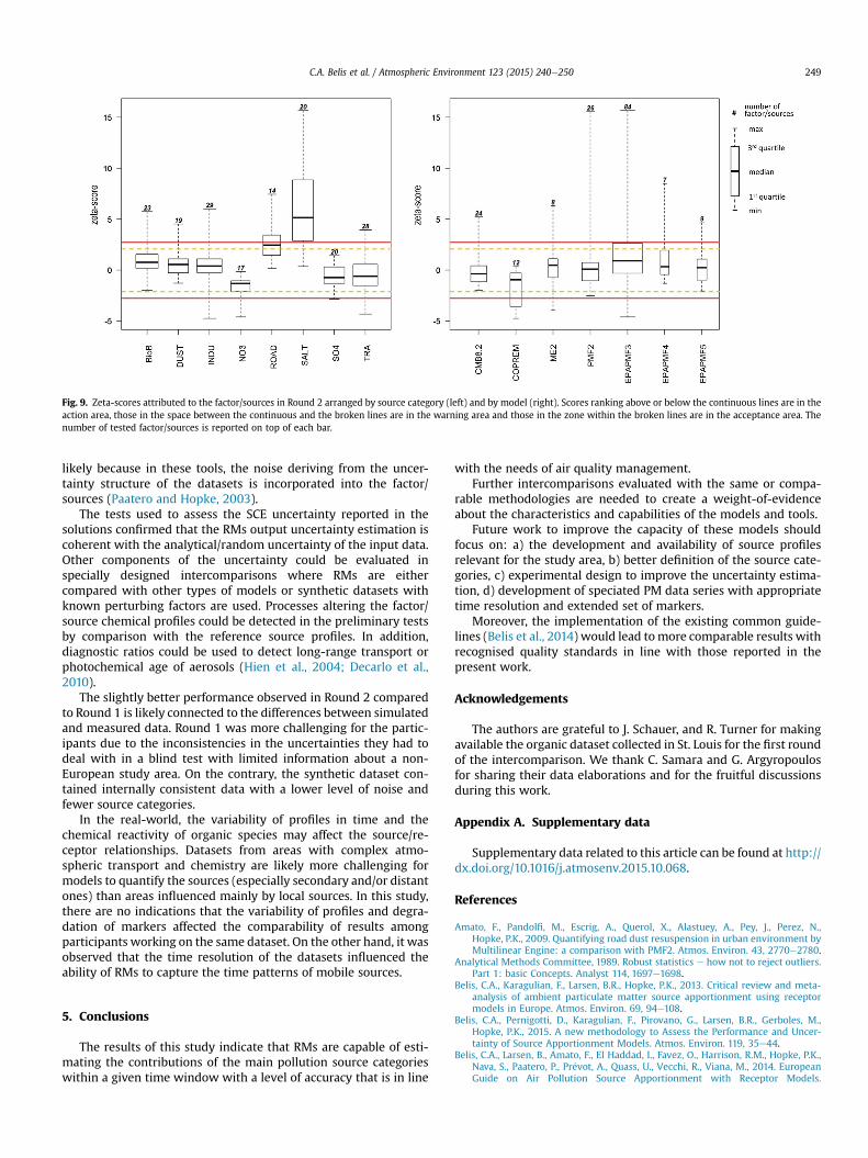
The mean of the reported relative standard uncertainties for theSCE of the whole timewindow in Round 2 is 13%. The lowest valuesare those in NO3 source categories and the highest are those inINDU. As for the models, the lowest uncertainties are those re-ported in ME-2 and CMB8.2 solutions and the highest are those ofCOPREM solutions. No uncertainty was reported for the SCEs ob-tained with FA-MLRA. The uncertainty attributed to the referencewas equivalent to the noise introduced in the synthetic dataset(20% standard deviation) that was derived from the analytical un-certainty in the input dataset (Belis et al., 2015). The zeta-score testindicates that a 68% of the declared factor/source SCE uncertaintiesare coherent with the one of the reference while a 19%, ranking inthe action area, are likely underestimated (Fig. 9).
SALT is the only source category with the majority of the zeta-scores in the action area (75%). Likely, models do not allow forthe higher relative uncertainty due the very low SCEs in this sourcecategory compared to the others. Uncertainty underestimation isobserved also in ROAD, which shows a 60% of the scores either inthe warning or in the action areas.
A considerable proportion of factor/sources obtained withEPAPMF4 and EPAPMF3 show underestimated uncertainties (29%
and 24% of scores in the action area, respectively). COPREM showeduncertainties higher than the reference in a 31% of the factor/sources. The satisfactory performance of CMB8.2 (more than 90%successful scores) suggests that propagating the uncertainty of thesource profiles can provide a satisfactory estimation of the SCEsuncertainty.
3.3.4. The impact of the operatorThe variability between solutions obtained by different practi-
tioners using the same tool and the same input data are an indicatorof the maximum impact of the operator subjectivity on the repro-ducibility. The tools with the highest number of reported solutions:EPAPMF3, PMF2, and CMB8.2 present a high consistency amongsolutions obtained by different practitioners using the same tool.The standard deviations of the SCE mean in each of these modelsranges between 0.2 and 0.3 mg/m3 and 1.4e1.7 mg/m3, in the firstand second rounds, respectively. These values are, in addition, closeto the standard deviation of the overall mean (0.2 mg/m3 and 1.7 mg/m3, in the first and second rounds, respectively). These resultssuggest a limited impact of the practitioners' subjectivity, onaverage. However, “outliers” were often associated with lessexperienced practitioners in terms of both years of use of the tooland number of studies performed.
4. Key findings of the intercomparison
The tests on chemical profiles confirmed, in themajority of cases(83%), the attribution of factors/profiles to source categories in thereported results and the majority of the SCEs (87%) reported byparticipants met the 50% standard uncertainty quality objectiveestablished for the performance test. A high share of the testedsolutions (70%e80%) apportioned a considerable amount of thePM2.5 mass to its pollution sources and many solutions estimated anumber of sources close to the expected value.
In this study, the estimation of source contribution was mostcritical for SALT, DUST, SHIP and categories associated with mobilesources. The majority of the solutions overestimated the SCE ofSALT, a source category with a contribution of about 1% of the PMmass. Such relative contribution may be considered a firstapproximation of the lower limit that the tested methodologies areable to quantify. Poor scores attributed to some DUST and ROADSCEs were ascribed to the similarities in the chemical compositionbetween road dust and crustal material that may have interferedwith the allocation of mass between these sources. The uncorre-lated time trends and, in some cases, the heterogeneous chemicalprofiles observed in INDU and SHIP were attributed to the lack of acommon definition of these categories. Sources with appreciablecontributions and chemical profiles dominated by few species, suchas NO3 and SO4, were more efficiently recognised by the modelseven though there was a tendency to slightly underestimate theirSCEs.
The most commonly used models, EPAPMF3, PMF2, and CMB8.2showed quite satisfactory performance with successful z-scoresranging between 80% and 100%. The good agreement between CMBand PMF may be partially due to the main RM assumptions beingsubstantially respected in the used datasets: limited alteration ofthe species between source and receptor and relatively stablesource profiles. In addition, both types of tools account for theuncertainties in the input data, have built-in performance in-dicators and have been available long enough to allow a widenumber of practitioners be familiar with them. For those modelsused in a limited number of solutions, only preliminary conclusionscan be drawn at this stage. In general, fully unconstrained modelswhich do not account for the input data uncertainty (e.g. FA-MLRAand APCFA) showed performances below the average. This result is
Fig. 9. Zeta-scores attributed to the factor/sources in Round 2 arranged by source category (left) and by model (right). Scores ranking above or below the continuous lines are in theaction area, those in the space between the continuous and the broken lines are in the warning area and those in the zone within the broken lines are in the acceptance area. Thenumber of tested factor/sources is reported on top of each bar.
likely because in these tools, the noise deriving from the uncer-tainty structure of the datasets is incorporated into the factor/sources (Paatero and Hopke, 2003).
The tests used to assess the SCE uncertainty reported in thesolutions confirmed that the RMs output uncertainty estimation iscoherent with the analytical/random uncertainty of the input data.Other components of the uncertainty could be evaluated inspecially designed intercomparisons where RMs are eithercompared with other types of models or synthetic datasets withknown perturbing factors are used. Processes altering the factor/source chemical profiles could be detected in the preliminary testsby comparison with the reference source profiles. In addition,diagnostic ratios could be used to detect long-range transport orphotochemical age of aerosols (Hien et al., 2004; Decarlo et al.,2010).
The slightly better performance observed in Round 2 comparedto Round 1 is likely connected to the differences between simulatedand measured data. Round 1 was more challenging for the partic-ipants due to the inconsistencies in the uncertainties they had todeal with in a blind test with limited information about a non-European study area. On the contrary, the synthetic dataset con-tained internally consistent data with a lower level of noise andfewer source categories.
In the real-world, the variability of profiles in time and thechemical reactivity of organic species may affect the source/re-ceptor relationships. Datasets from areas with complex atmo-spheric transport and chemistry are likely more challenging formodels to quantify the sources (especially secondary and/or distantones) than areas influenced mainly by local sources. In this study,there are no indications that the variability of profiles and degra-dation of markers affected the comparability of results amongparticipants working on the same dataset. On the other hand, it wasobserved that the time resolution of the datasets influenced theability of RMs to capture the time patterns of mobile sources.
5. Conclusions
The results of this study indicate that RMs are capable of esti-mating the contributions of the main pollution source categorieswithin a given time window with a level of accuracy that is in line
with the needs of air quality management.Further intercomparisons evaluated with the same or compa-
rable methodologies are needed to create a weight-of-evidenceabout the characteristics and capabilities of the models and tools.
Future work to improve the capacity of these models shouldfocus on: a) the development and availability of source profilesrelevant for the study area, b) better definition of the source cate-gories, c) experimental design to improve the uncertainty estima-tion, d) development of speciated PM data series with appropriatetime resolution and extended set of markers.
Moreover, the implementation of the existing common guide-lines (Belis et al., 2014) would lead tomore comparable results withrecognised quality standards in line with those reported in thepresent work.
Acknowledgements
The authors are grateful to J. Schauer, and R. Turner for makingavailable the organic dataset collected in St. Louis for the first roundof the intercomparison. We thank C. Samara and G. Argyropoulosfor sharing their data elaborations and for the fruitful discussionsduring this work.
Appendix A. Supplementary data
Supplementary data related to this article can be found at http://dx.doi.org/10.1016/j.atmosenv.2015.10.068.
References
Amato, F., Pandolfi, M., Escrig, A., Querol, X., Alastuey, A., Pey, J., Perez, N.,Hopke, P.K., 2009. Quantifying road dust resuspension in urban environment byMultilinear Engine: a comparison with PMF2. Atmos. Environ. 43, 2770e2780.
Analytical Methods Committee, 1989. Robust statistics e how not to reject outliers.Part 1: basic Concepts. Analyst 114, 1697e1698.
Belis, C.A., Karagulian, F., Larsen, B.R., Hopke, P.K., 2013. Critical review and meta-analysis of ambient particulate matter source apportionment using receptormodels in Europe. Atmos. Environ. 69, 94e108.
Belis, C.A., Pernigotti, D., Karagulian, F., Pirovano, G., Larsen, B.R., Gerboles, M.,Hopke, P.K., 2015. A new methodology to Assess the Performance and Uncer-tainty of Source Apportionment Models. Atmos. Environ. 119, 35e44.
Belis, C.A., Larsen, B., Amato, F., El Haddad, I., Favez, O., Harrison, R.M., Hopke, P.K.,Nava, S., Paatero, P., Pr�evot, A., Quass, U., Vecchi, R., Viana, M., 2014. EuropeanGuide on Air Pollution Source Apportionment with Receptor Models.
C.A. Belis et al. / Atmospheric Environment 123 (2015) 240e250250
Publication Office of the European Union, Italy, p. 88.Decarlo, P.F., Ulbrich, I.M., Crounse, J., De Foy, B., Dunlea, E.J., Aiken, A.C., Knapp, D.,
Weinheimer, A.J., Campos, T., Wennberg, P.O., Jimenez, J.L., 2010. Investigationof the sources and processing of organic aerosol over the Central MexicanPlateau from aircraft measurements during MILAGRO. Atmos. Chem. Phys. 10,5257e5280.
Favez, O., El Haddad, I., Piot, C., Bor�eave, A., Abidi, E., Marchand, N., Jaffrezo, J.L.,Besombes, J.L., Personnaz, M.B., Sciare, J., Wortham, H., George, C., D'anna, B.,2010. Inter-comparison of source apportionment models for the estimation ofwood burning aerosols during wintertime in an Alpine city (Grenoble, France).Atmos. Chem. Phys. 10, 5295e5314.
Friedlander, S.K., 1973. Chemical element balances and identification of air pollutionsources. Environ. Sci. Technol. 7, 235e240.
Galarneau, E., 2008. Source specificity and atmospheric processing of airbornePAHs: implications for source apportionment. Atmos. Environ. 42, 8139e8149.
Hien, P.D., Bac, V.T., Thinh, N.T.H., 2004. PMF receptor modelling of fine and coarsePM10 in air masses governing monsoon conditions in Hanoi, northern Vietnam.Atmos. Environ. 38, 189e201.
Hopke, P.K., 2010. The application of receptor modeling to air quality data. Pollut.Atmos. 91e109.
Hopke, P.K., Ito, K., Mar, T., Christensen, W.F., Eatough, D.J., Henry, R.C., Kim, E.,Laden, F., Lall, R., Larson, T.V., Liu, H., Neas, L., Pinto, J., St€olzel, M., Suh, H.,Paatero, P., Thurston, G.D., 2006. PM source apportionment and health effects:1. Intercomparison of source apportionment results. J. Expo. Sci. Environ. Epi-demiol. 16, 275e286.
ISO 13528, 2005. Statistical Methods for Use in Proficiency Testing by Interlabor-atory Comparisons. (ISO) International Organization for Standardization.
Jaeckels, J.M., Bae, M.S., Schauer, J.J., 2007. Positive matrix factorization (PMF)analysis of molecular marker measurements to quantify the sources of organicaerosols. Environ. Sci. Technol. 41, 5763e5769.
Jolliff, J.K., Kindle, J.C., Shulman, I., Penta, B., Friedrichs, M.A.M., Helber, R.,Arnone, R.A., 2009. Summary diagrams for coupled hydrodynamic-ecosystemmodel skill assessment. J. Mar. Syst. 76, 64e82.
Karagulian, F., Belis, C.A., 2012. Enhancing source apportionment with receptormodels to foster the air quality directive implementation. Int. J. Environ. Pollut.
Pandolfi, M., Viana, M., Minguill�on, M.C., Querol, X., Alastuey, A., Amato, F.,Celades, I., Escrig, A., Monfort, E., 2008. Receptor models application to multi-year ambient PM10 measurements in an industrialized ceramic area: compari-son of source apportionment results. Atmos. Environ. 42, 9007e9017.
Schauer, J.J., Rogge, W.F., Hildemann, L.M., Mazurek, M.A., Cass, G.R., Simoneit, B.R.T.,1996. Source apportionment of airborne particulate matter using organiccompounds as tracers. Atmos. Environ. 30, 3837e3855.
Thomson, M., Ellison, S.L.R., Wood, R., 2006. The international harmonized protocolfor the proficiency testing of analytical chemistry laboratories. Pure Appl. Chem.78, 145e196.
Thurston, G.D., Spengler, J.D., 1985. A quantitative assessment of source contribu-tions to inhalable particulate matter pollution in metropolitan Boston. Atmos.Environ. Part A General Top. 19, 9e25.
Viana, M., Kuhlbusch, T.A.J., Querol, X., Alastuey, A., Harrison, R.M., Hopke, P.K.,Winiwarter, W., Vallius, M., Szidat, S., Pr�evot, A.S.H., Hueglin, C., Bloemen, H.,Wåhlin, P., Vecchi, R., Miranda, A.I., Kasper-Giebl, A., Maenhaut, W.,Hitzenberger, R., 2008a. Source apportionment of particulate matter in Europe:a review of methods and results. J. Aerosol Sci. 39, 827e849.
Viana, M., Pandolfi, M., Minguill�on, M.C., Querol, X., Alastuey, A., Monfort, E.,Celades, I., 2008b. Inter-comparison of receptor models for PM source appor-tionment: case study in an industrial area. Atmos. Environ. 42, 3820e3832.
Viana, M., Hammingh, P., Colette, A., Querol, X., Degraeuwe, B., Vlieger, I.D., VanAardenne, J., 2014. Impact of maritime transport emissions on coastal air qualityin Europe. Atmos. Environ. 90, 96e105.
Watson, J.G., Chen, L.W.A., Chow, J.C., Doraiswamy, P., Lowenthal, D.H., 2008. Sourceapportionment: findings from the U.S. supersites program. J. Air Waste Manag.Assoc. 58, 265e288.