51
A New Route to Increasing Economic Growth Reducing Highway Congestion with Autonomous Vehicles Clifford Winston and Quentin Karpilow January 2017 MERCATUS WORKING PAPER
| Date post: | 20-Apr-2018 |
| Category: |
Documents |
| Upload: | hoanghuong |
| View: | 217 times |
| Download: | 2 times |
A New Route to Increasing Economic Growth
Reducing Highway Congestion with
Autonomous Vehicles
Clifford Winston and Quentin Karpilow
January 2017
MERCATUS WORKING PAPER
Clifford Winston and Quentin Karpilow. “A New Route to Increasing Economic Growth: Reducing Highway Congestion with Autonomous Vehicles.” Mercatus Working Paper, Mercatus Center at George Mason University, January 2017. Abstract This paper argues that California’s self-help county tax legislation, which funds additional highway spending, amounts to a natural experiment that can be used to construct a valid instrument to determine highway congestion’s causal effect on the growth rates of GDP, employment, wages, and commodity freight flows for California counties. Our estimation results indicate that highway congestion has significantly reduced the growth rates of those performance measures. Extrapolating the results to the nation suggests that sizable reductions in highway congestion, which could be achieved with widespread adoption of autonomous (driverless) vehicles, would have large macroeconomic stimulative effects. JEL codes: R1, R41, H71 Keywords: congestion delays, autonomous vehicles, driverless vehicles, self-help county taxes Author Affiliation and Contact Information Clifford Winston Searle Freedom Trust Senior Fellow Economic Studies Senior Fellow Brookings Institution [email protected] Quentin Karpilow JD candidate 2018 Yale University [email protected] All studies in the Mercatus Working Paper series have followed a rigorous process of academic evaluation, including (except where otherwise noted) at least one double-blind peer review. Working Papers present an author’s provisional findings, which, upon further consideration and revision, are likely to be republished in an academic journal. The opinions expressed in Mercatus Working Papers are the authors’ and do not represent official positions of the Mercatus Center or George Mason University.
3
A New Route to Increasing Economic Growth
Reducing Highway Congestion with Autonomous Vehicles
Clifford Winston and Quentin Karpilow
1. Introduction
Because highway congestion significantly increases travel times and makes travel times less
reliable, it can adversely affect key sectors of an economy and its aggregate performance by
constraining individuals’ ability to work, earn, consume, and produce. For example, Amiti et al.
(2015) calculated that congestion at the nation’s West Coast ports, which occurred from July
2014 through February 2015 while dockworkers and marine terminal employers were
negotiating a contract, caused perishable agricultural commodities to go bad, thus resulting in a
0.2 percentage point reduction in GDP growth during the first quarter of 2015. Hymel (2009),
Sweet (2014), and Angel and Blei (2015) have found that highway congestion is associated with
slower job growth in US metropolitan areas. Light (2007) used the Bureau of Labor Statistics
American Time Use Survey to estimate reductions in workers’ productivity and income that are
caused by traffic delays from highway congestion.
This fragmentary evidence indicates the importance of having a comprehensive picture
of the effects of highway congestion on an economy. We provide this picture by estimating the
causal effect of highway congestion on the growth rates of several different measures of
economic performance, including GDP, employment, wages, and commodity freight flows, for
certain congested California counties. We focus our empirical analysis on California because it
has several highly congested urban areas, including 11 of the top 16 highway bottlenecks in the
nation (CPCS Transcom 2015), and because its counties have had, since the early 1960s, the
4
option to pass local sales taxes to fund spending for specific highway projects that could
reduce congestion.1
We argue that such duly named self-help taxes amount to a so-called natural experiment
because they have been enacted at various times by various counties primarily because of
political considerations, rather than because of economic factors relevant to economic growth.
Accordingly, our identification strategy is to use the additional highway spending that is funded
by self-help tax legislation as a valid instrument to determine the causal effect of highway
congestion on measures of economic performance.
Our estimation results indicate that highway congestion has had large adverse effects on
the growth rates of GDP, employment, labor earnings, and commodity freight flows for the
congested California counties in our sample. We consider how these growth rates could be
revitalized by actions that reduce congestion. Economists have long recommended charging
highway tolls during peak travel periods as an efficient approach to the problem of highway
congestion. But so-called congestion pricing increases the monetary cost of commuting to work;
thus, it is not clear that using this price tool to reduce congestion would unambiguously increase
employment and other measures of economic activity, although it would increase government
revenue and economic welfare.
In contrast, widespread adoption of autonomous (driverless) vehicles—which American
and foreign technology companies and automakers are actively developing, testing, and
perfecting, with some industry leaders and US Secretary of Transportation Anthony Foxx
1 Istrate, Nowakowski, and Mak (2014) discuss county funding of transportation. They point out that counties are increasingly using local-option sales taxes to fund transportation projects, if those taxes are permitted under state law. As of this writing, county residents in 15 states, including California, have voted for local-option sales taxes for road projects.
5
expecting driverless vehicles to be available to the public by 2021—could reduce highway
congestion by greatly improving the flow of traffic and by reducing vehicle accidents without
significantly increasing the monetary cost of commuting.2 Using our estimation results for
California and conservatively extrapolating to the nation, we find that the adoption of
autonomous vehicles could have potentially large macroeconomic stimulative effects.
Specifically, in a given year, a 50 percent penetration rate for autonomous vehicles (i.e., half of
the vehicles used by motorists would be driverless) could add at least $214 billion in GDP, 2.4
million jobs, and $90 billion in income to the US labor force.
Policymakers’ preferred strategy to reduce highway congestion—that of raising funds to
expand road capacity—has failed to achieve a consensus in Congress and has been rejected by
many economists as often wasteful and more likely to result in additional highway traffic that
would quickly fill new roads to capacity (Duranton and Turner 2011, Winston 2013). However,
policymakers can play a constructive role in reducing congestion and can contribute a
surprisingly large stimulus to the economy by facilitating manufacturers’ introduction and
motorists’ adoption of autonomous vehicles.
2 New developments are announced every month about the intense global race involving major US and foreign automakers, major technology companies (including Google and Baidu), start-up automobile technology companies, and ridesharing companies to develop autonomous vehicles and have them adopted by motorists. A definitive date for widespread adoption is not available, but Uber has begun a public trial of autonomous (ridesharing) vehicles in Pittsburg, NuTonomy has begun a public trial of autonomous taxis in Singapore, and Boston was chosen by the World Economic Forum to be the test city for autonomous vehicles in 2017. The additional cost of autonomous vehicles over current nonautonomous vehicles will decline sharply over time and will represent only a modest increase in the purchase price of a new car as market penetration of autonomous vehicles increases.
In the policy community, the Obama administration has announced guidelines for the development and use of autonomous vehicles, outlining safety expectations and encouraging uniform rules nationwide. To be sure, there are critics of the new technology. Kalra and Paddock (2016) argue that autonomous vehicles would have to travel hundreds of millions (possibly hundreds of billions) of miles before their reliability and safety could be fully determined. But their study assumes that the software and technology are static and also ignores suppliers’ steep learning curve, where mistakes will be quickly identified and corrected, and some vehicles will learn from other vehicles’ experiences. Generally, critics and advocates alike should accept that problems will occur along the way toward adopting driverless technology but that suppliers will work hard to respond to the problems and improve safety and reliability. At the same time, users must accept that it will take time for them to be comfortable with the new technology.
6
2. Framework and Data
Traditional efficiency analyses of highway congestion measure the delay costs that motorists
who travel during peak travel periods impose on other motorists.3 But the economic effects of
congestion go far beyond those social costs because an efficient transportation system expands
individuals’ access to and choices of employers; enables firms and urban residents to benefit
from the spatial concentration of economic activities, referred to as agglomeration economies;
and reduces trade costs and allows firms to realize efficiency gains from specialization,
comparative advantage, and increasing returns (Winston 2013).
By increasing travel time and making it less reliable (Small, Winston, and Yan 2005),
congestion can erode those benefits, as documented by the following empirical studies. Chetty et
al. (2014) find that longer commuting times are strongly and negatively related to the probability
that a household will escape poverty, implying that congestion adversely affects employment and
job opportunities, especially for low-income workers. Puga (2010) summarizes the evidence that
urban density contributes to agglomeration economies and higher earnings; thus, congestion may
reduce those economies because it increases the time that commuters must travel to access
employment opportunities. For example, Prud’homme and Lee (1999) estimate that a region’s
productivity decreases 1.3 percent when the area that can be reached in a given time period
decreases 10.0 percent. And Anderson and van Wincoop (2004) conclude that travel distance and
time represent important components of trade costs; thus, congestion may increase those costs
and decrease trade flows.
3 The costs are shown in the conventional diagram to analyze congestion (Lindsey 2006, Winston and Mannering 2014). Langer and Winston (2008) extend the framework to account for congestion’s effect on land use and residential location decisions.
7
To the best of our knowledge, no study has, to date, attempted to systematically measure
the direct impact of highway congestion on an economy’s overall health. We seek to do so by
using panel data to estimate the effect that highway congestion has on the economic performance
of urban areas in California, as measured by their GDP, employment, labor earnings, and trade
flow growth rates.4 Our general model is a reduced form that incorporates a complex interrelated
system of demand, congestion, and economic decisions. It can be described as
Git = f (Cit, Xit, εit), (1)
where Git is the growth rate of an economic performance variable in California urban area i during
year t, Cit is the level of congestion, Xit is an array of controls, and εit is a random error term.
Below, we summarize the available data to measure congestion and the dependent
variables in equation (1). We then describe and justify our instrument for congestion and the data
we use to measure it in the next section.
2.1. Congestion
We measure congestion using the Texas A&M Transportation Institute’s (TTI’s) estimates of
annual hours of delay per auto commuter (Schrank et al. 2015). Data are provided for the years
1982–2011 for all urban areas with more than 500,000 people. Auto commuters are defined as
people who make trips by car during morning and evening peak periods: 6–10 a.m. and 3–7 p.m.
The numbers of auto commuters are estimated using data from the Federal Highway
Administration’s (FHA) National Household Travel Survey (FHA 2009). TTI adds
measurements of peak-period delays to measurements of travel delay during nonpeak hours to
estimate the total annual delay experienced by auto commuters.
4 We also perform estimations using county-level data, which we discuss below.
8
To compute congestion-induced delays during both peak and nonpeak periods, TTI
estimates two speeds for a given roadway segment: (1) the free-flow speed, or the average speed
observed during light traffic periods of the day (e.g., 10 p.m.–5 a.m.), and (2) the actual speed
observed during a given time interval of the day. By comparing actual and free-flow speeds, TTI
is able to estimate congestion-induced speed reductions for different hours of the day. TTI then
scales up those speed reductions using traffic volume data to compute the total amount of time
“lost” to traffic congestion. In recent years, travel speed data have come from INRIX, a private
company that monitors travel times on most major roads in the United States. (TTI has made
considerable efforts to align earlier data with INRIX data.) Traffic volume data come from the
FHA’s Highway Performance Monitoring System (FHA 2015). Importantly, the INRIX speed
data are recorded in 15-minute intervals for every day of the year, thereby allowing TTI to
account for both daily and hourly variations in congestion levels.5 For our sample of California
urban areas during 1982–2011, which we discuss later, annual delay per auto commuter ranged
from 2 hours to 89 hours, with a mean delay of 34 hours per year.
2.2. Economic Performance Measures
We use county-level economic performance measures that include real GDP, wages,
employment, and originating freight traffic transported by truck. Real GDP, wages, and
employment data for 1982–2011 were provided by the Brookings Institution’s Metropolitan
Policy Program (Istrate, Berube, and Nadeau 2012), using data from Moody’s Analytics.6 Freight
5 Although it could be argued from a policy perspective that TTI’s benchmark of free-flow speeds is unlikely to be obtained during peak periods, TTI still offers a valid measure of delays caused by traffic congestion, and there is no clear alternative measure. More important, the introduction of autonomous vehicles offers the possibility of much higher speeds during peak periods. 6 The Moody’s Analytics source for employment and wage data is BLS (2016), and its source for GDP data is the Bureau of Economic Analysis.
9
flows, measured as thousands of tons of commodities transported by truck across California
counties, were obtained from the California Statewide Freight Forecasting Model, which
combines 2007 data from the FHA’s Freight Analysis Framework (FHA 2016) with
demographic data to forecast flows for 2010.7 The forecast flows are not adjusted to account for
any unanticipated changes in congestion.
We express GDP, wages, and employment in terms of annual growth rates as
!"#$%ℎ'() = ln ()-./()-
, (2)
where !"#$%ℎ'() is the annual growth rate of a dependent-variable performance measure DV in
year t, 12'34 is the level of the dependent variable DV in year t+1, and 12' is the level of the
dependent variable DV in year t.8 Because we have commodity flow data for the years 2007 and
2010 only, we express the dependent variable for this performance measure as a three-year
growth rate—the difference between 2010 and 2007 levels.
3. Identification Based on Self-Help County Taxes as an Instrument to Measure Highway
Congestion
There are two fundamental challenges to estimating the effect of congestion on an economic
performance measure (e.g., employment): omitted variables and reverse causality. Omitted
variables are likely to arise because some variables that affect both congestion and an economic
performance measure, such as certain types of weather (Sweet 2014), will be omitted from the
model because they are difficult to quantify. Reverse causality is likely to occur because an
7 We are grateful to Andre Tok and Stephen Ritchie, both from the Institute for Transportation Studies, for providing us with these data. Details on the design and development of the California Statewide Freight Forecasting Model are contained in Ranaiefar (2014) and Ranaiefar et al. (2012). 8 Note that ln(DVt+1/DVt) = ln[1+(DVt+1−DVt)/DVt] ≈ (DVt+1−DVt)/DVt when (DVt+1−DVt)/DVt is small.
10
economic performance measure will be closely related to the amount of passenger and freight
traffic on the road and thus will affect congestion. The standard approach to minimizing the bias
from omitted variables and reverse causality is to use an appropriate instrumental variable that is
correlated with the explanatory variable of interest (in this case, highway congestion) but is not
correlated with the dependent variable (e.g., employment).
Starting in the 1960s, California counties were allowed by state law to pass legislation,
with voter approval, that instituted local sales taxes to fund transportation projects that would,
among other things, help reduce highway congestion.9 Based on considerable evidentiary and
institutional support that we provide below, we contend that the share of the local sales tax base
dedicated to self-help highway projects—that is, counties that opt to help themselves by raising
transportation funding locally—is a valid instrument for highway congestion.
In contrast to conventional models in public finance, we argue that the revenue raised by
self-help county taxes for highway projects is not the result of welfare-maximizing decisions by
policymakers subject to current economic conditions; instead, it is determined primarily by
county leaders’ effectiveness at mobilizing the political support of a clear majority of voters,
which bears little relationship to a county’s current economic conditions. Li, Linn, and
Muehlegger (2014) discuss the evidence on political considerations that affect state gasoline
taxes. Interestingly, the failure of congressional leaders to mobilize political support to raise the
national gasoline tax has maintained the tax rate at its 1993 level, despite varying
macroeconomic conditions. This static tax rate has contributed to large shortfalls in the FHA’s
Highway Trust Fund, which pays for road maintenance and improvements (Langer, Maheshri,
and Winston 2016). Similarly, although California’s cost of borrowing has fallen significantly, a
9 California counties did not tend to allocate a notable share of the sales taxes to highways until the 1980s.
11
political trend toward antitax sentiment has led the state’s transportation officials to cut highway
construction plans by 28 percent between 2016 and 2021 (Harrison and Gillers 2016).
We use data on self-help county taxes from the website of each of the California counties
in our analysis sample and from an initial summary by Crabbe et al. (2005).10 Counties vary by
(1) the years during which they vote on, pass, and renew a transportation sales tax; (2) the sales
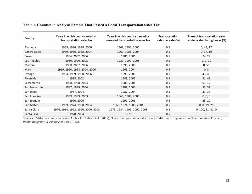
tax rate; and (3) the share of the transportation tax revenue dedicated to highways. Table 1 shows
the factors that contribute to the variation in California counties’ accumulation of highway tax
revenue over time by listing the preceding information for the counties with measurable
congestion that passed transportation sales taxes.11 The share of self-help revenue going to
highway projects varies noticeably, ranging from 0 percent (none of the self-help revenue funds
highway work) to 100 percent (all of the self-help revenue funds highway work).
10 We are grateful to Amber Crabbe of the Transportation and Land Use Coalition for providing the data. 11 Notably, some counties—such as Sonoma—have passed a transportation tax rate other than 0.5 percent, but those counties do not have measurable congestion, so their tax rates do not appear in our table.
12
Table 1. Counties in Analysis Sample That Passed a Local Transportation Sales Tax
County Yearsinwhichcountyvotedontransportationsalestax
Yearsinwhichcountypassedorrenewedtransportationsalestax
Transportationsalestaxrate(%)
Shareoftransportationsalestaxdedicatedtohighways(%)
Alameda 1969,1986,1998,2000 1969,1986,2000 0.5 0,43,17ContraCosta 1969,1986,1988,2004 1969,1988,2004 0.5 0,37,19Fresno 1986,2002,2006 1986,2006 0.5 74,29LosAngeles 1980,1990,2008 1980,1990,2008 0.5 0,0,20Madera 1990,2002,2006 1990,2006 0.5 0,51Marin 1969,1990,1998,2004,2006 1969,2004 0.5 0,8Orange 1984,1989,1990,2006 1990,2006 0.5 43,43Riverside 1988,2002 1988,2002 0.5 51,43Sacramento 1988,1988,2004 1988,2004 0.5 63,12SanBernardino 1987,1989,2004 1989,2004 0.5 53,37SanDiego 1987,2004 1987,2004 0.5 33,33SanFrancisco 1969,1989,2003 1969,1989,2003 0.5 0,0,0SanJoaquin 1990,2006 1990,2006 0.5 25,20SanMateo 1969,1974,1988,2004 1969,1974,1988,2004 0.5 0,0,29,28SantaClara 1976,1984,1992,1996,2000,2008 1976,1984,1996,2000,2008 0.5 0,100,31,31,0SantaCruz 1978,2004 1978 0.5 0
Sources: California county websites; Amber E. Crabbe et al. (2005), “Local Transportation Sales Taxes: California’s Experiment in Transportation Finance,” Public Budgeting & Finance 25 (3): 91–121.
13
Self-help ballot measures come with specific expenditure plans detailing how revenue
from the taxes will be spent. Many highway projects are expensive, and it can take considerable
time for a county’s self-help tax to raise the funds necessary to complete a project designed to
reduce congestion; thus, we express our instrument for congestion in a county as the cumulative
share of the county sales tax base that is spent on self-help highway projects,
!"#"$%&'()*'+ℎ-%./ℎ%0)12, which we express as
!"#"$%&'()*'+ℎ-%./ℎ%0)12 = &%45%&)16 ∗ %ℎ'+ℎ-%.16,26:;<=> (3)
where &%45%&)16 is the local transportation tax rate for county i in year j (e.g., 0.50 or 0.25
percent),12 and %ℎ'+ℎ-%.16 is the share of self-help county tax revenue that is allocated to
highway projects in year j, as stipulated by the expenditure plan developed by county i. We
discuss additional reasons for using a cumulative measure below.
For short, we will refer to this construct as the cumulative share of the self-help tax base
dedicated to highways. Consider, for example, Fresno County. In 1986, Fresno began imposing a
0.5 percent transportation sales tax, 74 percent of which went to highway projects. Thus, 0.37
percent of the county’s sales tax base went to self-help highway projects in 1986. An additional
0.37 percent did so in 1987, meaning that 0.74 percent of the cumulative tax base since 1982 (the
starting year of our sample) went to highways by 1987. In other words,
!"#"$%&'()*'+ℎ-%./ℎ%0)?@ABCD,;<=E = 0%,
!"#"$%&'()*'+ℎ-%./ℎ%0)?@ABCD,;<=G = 0.37%,
!"#"$%&'()*'+ℎ-%./ℎ%0)?@ABCD,;<=K = 0.74%,
and so forth.
12 California’s 1971 Transportation Development Act allows any California county to impose a 0.25 percent sales tax, subject to voter approval, for transportation purposes. Subsequently, Sonoma County passed a self-help transportation tax rate of 0.25 percent in 2004.
14
We discuss alternative ways of specifying this instrument later, but we note here that we
do not use the actual dollar amount of highway revenues from self-help taxes as an instrument
because dollar amounts are a function of the size of the economy, which is endogenous.13
Because expenditure plans may change when counties vote to renew a self-help tax,
&%45%&)16 and %ℎ'+ℎ-%.16 may vary across years. In the years preceding the enactment of a
self-help tax measure and in the years following the discontinuation of a self-help tax measure,
&%45%&)16 and %ℎ'+ℎ-%.16 are set to 0.
By using a cumulative measure of the share of the local sales tax base going to self-help
highway projects, we are able to account for (1) lags between revenue intake and transportation
expenditures, (2) differences in the rate at which counties accumulate self-help transportation
funds, and (3) the modest amount of revenue for highway projects that a county can accumulate
each year from a self-help tax compared with the high cost of certain highway projects. For
example, in 2014, the majority of counties received less than $100 million in total self-help tax
revenue (California Department of Transportation 2014), compared with an average construction
cost of more than $100 million for 10 miles of urban highway.
How do we justify treating the self-help county taxes as exogenous to our economic
performance measures?14 The exogeneity of &%45%&)16 is self-evident because there is almost no
variation in &%45%&)16 across either time or counties. Specifically, every county has a self-help
13 Returning to the example of Fresno County, the revenue raised by Fresno’s self-help tax may vary from year to year, reflecting changes in consumer spending habits or the strength of the economy. However, the annual share of that revenue going to highways (74 percent) remains constant, reflecting only the initial (and, we argue, exogenous) decision to allocate self-help funds among various transportation projects. 14 We are not aware of a formal econometric test of our instrument’s validity. Kitagawa (2015) has proposed a test of an instrument’s validity when both the variable of interest and the instrument are discrete. However, we cannot use that method here because congestion and the cumulative share of county sales taxes spent on self-help highway projects are continuous variables.
15
transportation tax of 0.5 percent, with the exception of Sonoma, which has a rate of 0.25 percent
and is not included in TTI’s sample of the most congested urban areas in the country.15
Among those counties in our study that eventually passed a self-help tax measure, we
argue that both the year in which a transportation tax was enacted and the share of self-help tax
revenue dedicated to highway projects are exogenous to economic trends and conditions in the
county. We offer several pieces of macro- and microempirical and institutional evidence to
support this claim.
First, our sample of California urban areas includes only those that are in TTI’s sample of
the most congested urban areas in the United States from 1982 to 2011; thus, those areas
experienced congestion throughout the period covered by our sample, and they were not
subjected to an economic “shock” that caused their residents to suddenly become concerned
about congestion and to enthusiastically support additional taxes to reduce it.
Second, it is possible that either the timing of a self-help tax or the share dedicated to
highway projects is driven by earlier economic or congestion trends. For example, if a county
observed that congestion levels were rising rapidly, that county might have been more likely to
pass a self-help tax or to dedicate a larger share of self-help tax revenue to highway projects. In
other words, in our sample, policymakers may have been responding to historic trends in
congestion when making self-help tax decisions. Although our model contains dummies for year
and urban area, it does not control for time-varying trends within an urban area, including the
hypothetical correlation between self-help taxes and within-county congestion trends.
15 Voting records for Sonoma show that earlier self-help county ballots—which proposed a variety of different tax rates—did not result in dramatically different voting outcomes. This suggests that Sonoma’s 0.25 percent tax rate is not due to an extreme antitax environment.
16
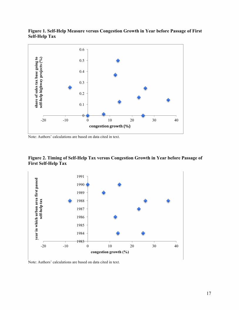
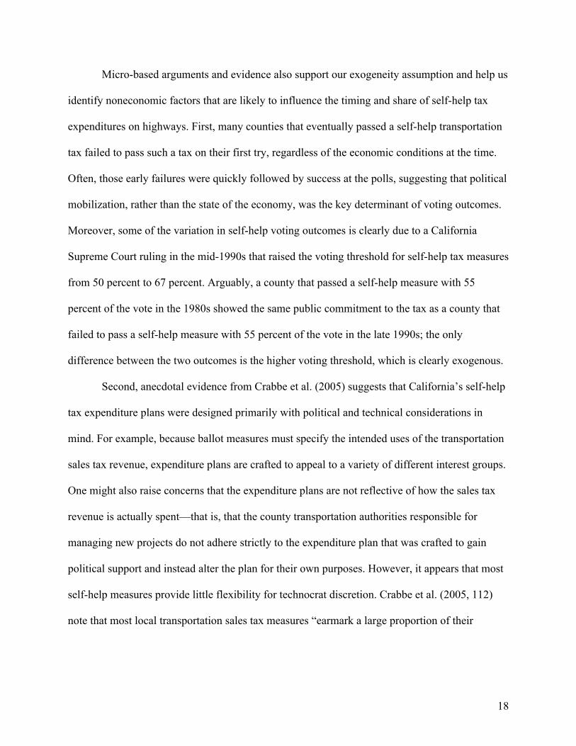
To test whether such a correlation exists, we computed the congestion growth rate for the
year before the passage of an urban area’s first self-help tax.16 Because there are only 10
California urban areas in our final sample, we simply mapped this measure of pre–self-help tax
annual congestion growth rates onto (1) the share of an urban area’s sales tax base going to
highway projects (i.e., our self-help instrument) and (2) the year in which the urban area first
passed a self-help tax. As shown in figures 1 and 2, neither the share of revenue going to self-
help highway projects nor the timing of the passage of a self-help tax appears to correlate with
congestion trends preceding the enactment of a self-help measure. Similar findings were
obtained when we considered annual GDP, instead of congestion, growth rates for the year
before the passage of the first self-help tax.17
Finally, because economic outcomes, congestion, and cumulative self-help county tax
expenditures may have a common time trend at the local (county) level owing to, for example,
natural events such as an earthquake that may affect only certain counties in California, we
conduct a sensitivity analysis by estimating our growth models with random time trend effects.
We find that controlling for those effects does not materially affect our parameter estimates.
16 Because we do not have pre-1982 congestion data, we define the first self-help tax as that which passed since 1982. For example, Alameda County passed a transportation sales tax in 1969, 1986, and 2000. For this analysis, we define Alameda’s first self-help measure as the one that passed in 1986. 17 We also find no correlation between the share of the tax base going to self-help highways and the level of congestion or the level of GDP that an urban area experienced during the year in which it passed its self-help tax measure. If underlying economic or congestion considerations motivated the allocation of self-help funds to highways, we might expect such a correlation to exist.
17
Figure 1. Self-Help Measure versus Congestion Growth in Year before Passage of First Self-Help Tax
Note: Authors’ calculations are based on data cited in text.
Figure 2. Timing of Self-Help Tax versus Congestion Growth in Year before Passage of First Self-Help Tax
Note: Authors’ calculations are based on data cited in text.
0
0.1
0.2
0.3
0.4
0.5
0.6
-20 -10 0 10 20 30 40
shar
e of
sale
s tax
bas
e go
ing
to
self-
help
hig
hway
pro
ject
s (%
)
congestiongrowth(%)
1983
1984
1985
1986
1987
1988
1989
1990
1991
-20 -10 0 10 20 30 40
year
in w
hich
urb
an a
rea
first
pas
sed
self-
help
tax
congestion growth (%)
18
Micro-based arguments and evidence also support our exogeneity assumption and help us
identify noneconomic factors that are likely to influence the timing and share of self-help tax
expenditures on highways. First, many counties that eventually passed a self-help transportation
tax failed to pass such a tax on their first try, regardless of the economic conditions at the time.
Often, those early failures were quickly followed by success at the polls, suggesting that political
mobilization, rather than the state of the economy, was the key determinant of voting outcomes.
Moreover, some of the variation in self-help voting outcomes is clearly due to a California
Supreme Court ruling in the mid-1990s that raised the voting threshold for self-help tax measures
from 50 percent to 67 percent. Arguably, a county that passed a self-help measure with 55
percent of the vote in the 1980s showed the same public commitment to the tax as a county that
failed to pass a self-help measure with 55 percent of the vote in the late 1990s; the only
difference between the two outcomes is the higher voting threshold, which is clearly exogenous.
Second, anecdotal evidence from Crabbe et al. (2005) suggests that California’s self-help
tax expenditure plans were designed primarily with political and technical considerations in
mind. For example, because ballot measures must specify the intended uses of the transportation
sales tax revenue, expenditure plans are crafted to appeal to a variety of different interest groups.
One might also raise concerns that the expenditure plans are not reflective of how the sales tax
revenue is actually spent—that is, that the county transportation authorities responsible for
managing new projects do not adhere strictly to the expenditure plan that was crafted to gain
political support and instead alter the plan for their own purposes. However, it appears that most
self-help measures provide little flexibility for technocrat discretion. Crabbe et al. (2005, 112)
note that most local transportation sales tax measures “earmark a large proportion of their
19
revenue for specific projects, limiting the power of transportation authorities to reprioritize once
the tax is approved.”
Finally, the prioritization of projects that are to be funded by self-help taxes appears to be
shaped by considerations that are orthogonal to performance measures of the economy. In
particular, Crabbe et al. (2005) write that the most common project prioritization criteria are
leveraging state and federal sources of funding, ensuring that sales tax revenue is distributed
fairly across all geographic subregions in a county, and satisfying established growth
management requirements for new development projects. Thus, in all such cases, bureaucratic
and political constraints appear to be shaping the order in which transportation projects that are
funded by county self-help revenue are implemented. Indeed, we show that the ability over time
of self-help transportation tax revenue to reduce highway congestion has varied greatly across
California counties, in all likelihood because different counties face different constraints and
have different goals when selecting highway projects.
It would be desirable to identify specific political variables that are unrelated to economic
conditions yet correlate with our instrument, but we are not aware of detailed case studies that
describe the political considerations that California counties have taken into account and the
specific strategies those counties have followed to select transportation projects and to gain voter
approval for proposed self-help transportation tax measures. However, consistent with Crabbe et
al. (2005), Sacramento County recently unveiled a list of proposed transportation projects,
including (1) all travel modes, even walking and cycling, and types of infrastructure; (2) every
city in the county, as well as unincorporated areas; and (3) an indication that the projects would
be funded in part with a new self-help county tax (Bizjak 2016). In addition, the list of projects
places a priority on those that would improve the county’s chances of receiving matching state
20
and federal funds. City and county leaders have indicated that polling in 2015 showed that
reaching the 67 percent approval threshold for a self-help tax could be tough to achieve and that
further voter polling would determine whether local leaders would formally launch the process to
put a self-help tax measure on the ballot in the future.
In sum, there is ample evidence to suggest that political considerations and bureaucratic
constraints are the primary determinants of when self-help taxes are passed in California counties
and how local tax revenue is spent. The fact that transportation authorities appear to have little
discretion during implementation of expenditure plans further strengthens our claim that county
self-help transportation taxes bear little relationship to the economic performance measures listed
earlier and are therefore a valid instrument for highway congestion in our empirical analysis.18
4. Constructing a Consistent Unit of Analysis and the Final Sample
The TTI data on average annual hours of delay per auto commuter are measured at the urban-
area level (Schrank et al. 2015). Data on urban-area economic characteristics, however, are
sparse; thus, Hymel (2009) and Sweet (2014), for example, rely on data for metropolitan
statistical areas (MSAs) to construct dependent variables that proxy for urban-area-level
economic conditions. It is not feasible for us to use MSA-level data here because the allocation
of self-help tax funds is decided at the county level, not the MSA level. This means that a county
must be the unit of analysis for our instrumental variable—the cumulative share of sales revenue
18 It could be argued that expenditures on highway maintenance and construction in an urban area follow a similar pattern as self-help highway tax expenditures and would therefore be a valid instrument for congestion. But those expenditures are affected to some extent by local economic activity that determines the amount of truck traffic. As discussed by Small, Winston, and Evans (1989), trucks are the primary cause of pavement damage, which requires ongoing maintenance and possibly new construction.
21
dedicated to self-help highway projects. In addition, we must rely on county-level data to
construct commodity flows and GDP.19
We therefore use county-level data to measure our dependent and instrumental variables
but then transform those county-level measures into urban-area measures to align them with our
congestion variable. Specifically, we apply the following transformation:
N6 = N1 ∗ O16,PQ
1:; (4)
where N6 is the measure of variable X for urban area R; N1 is the measure of variable X for county
'; O16 is the share of urban area R’s population that lived in county ' in 2010, as indicated by the
US Census; and S6 is the number of counties that overlap with urban area R.20 Thus, in all models
using annual growth rates for GDP, employment, and wages, the unit of analysis is the urban area.
Using the Bureau of Economic Analysis MSA-level data on employment and earnings for
the 1982–2011 time period, we perform robustness checks on whether the results of our jobs and
earnings growth models hold when we construct the dependent variable using MSA-level, as
opposed to county-level, growth rates. As noted later, we find that our results are robust to this
alternative specification, suggesting that our estimates of the effect of highway congestion on
employment and earnings are not driven by our reliance on county-level data.
We include freight flows across only California counties because our instrument for
congestion is valid only for California counties that had already voted for a self-help county tax
during the period studied. The implication of this restriction is that we understate the effect of
congestion on freight flows because we do not include its effect on flows between California
19 Furthermore, the Bureau of Economic Analysis provides MSA-level GDP data for the years 2001–2013, which would force us to drop all the years in our sample from the early 1980s to 2000. 20 Note that, for each urban area R, O16 = 1
PQ
1:;.
22
counties and US urban areas outside California or between California counties and foreign
urban areas.21
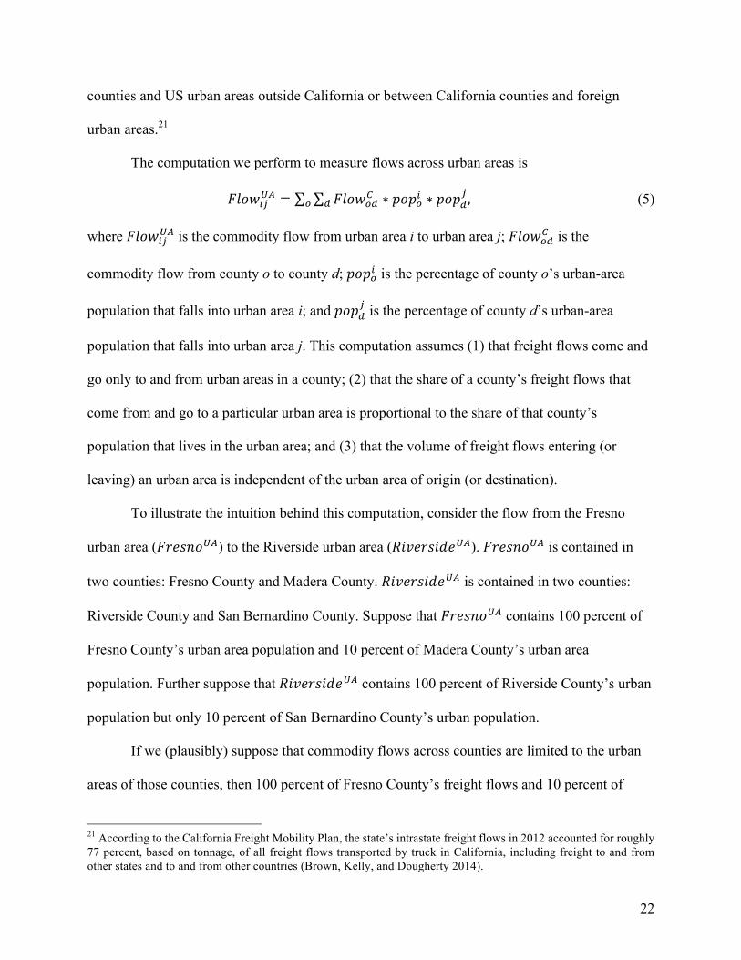
The computation we perform to measure flows across urban areas is
U$V-16WX= U$V-DY
Z∗ [V[D
1 ∗ [V[Y
6
YD , (5)
where U$V-16WX is the commodity flow from urban area i to urban area j; U$V-DYZ is the
commodity flow from county o to county d; [V[D1 is the percentage of county o’s urban-area
population that falls into urban area i; and [V[Y
6 is the percentage of county d’s urban-area
population that falls into urban area j. This computation assumes (1) that freight flows come and
go only to and from urban areas in a county; (2) that the share of a county’s freight flows that
come from and go to a particular urban area is proportional to the share of that county’s
population that lives in the urban area; and (3) that the volume of freight flows entering (or
leaving) an urban area is independent of the urban area of origin (or destination).
To illustrate the intuition behind this computation, consider the flow from the Fresno
urban area (U0)\]VWX) to the Riverside urban area (5'()0\'^)WX). U0)\]VWX is contained in
two counties: Fresno County and Madera County. 5'()0\'^)WX is contained in two counties:
Riverside County and San Bernardino County. Suppose that U0)\]VWX contains 100 percent of
Fresno County’s urban area population and 10 percent of Madera County’s urban area
population. Further suppose that 5'()0\'^)WX contains 100 percent of Riverside County’s urban
population but only 10 percent of San Bernardino County’s urban population.
If we (plausibly) suppose that commodity flows across counties are limited to the urban
areas of those counties, then 100 percent of Fresno County’s freight flows and 10 percent of
21 According to the California Freight Mobility Plan, the state’s intrastate freight flows in 2012 accounted for roughly 77 percent, based on tonnage, of all freight flows transported by truck in California, including freight to and from other states and to and from other countries (Brown, Kelly, and Dougherty 2014).
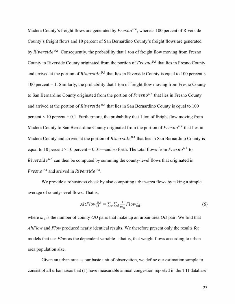
23
Madera County’s freight flows are generated by U0)\]VWX, whereas 100 percent of Riverside
County’s freight flows and 10 percent of San Bernardino County’s freight flows are generated
by5'()0\'^)WX. Consequently, the probability that 1 ton of freight flow moving from Fresno
County to Riverside County originated from the portion of U0)\]VWX that lies in Fresno County
and arrived at the portion of 5'()0\'^)WX that lies in Riverside County is equal to 100 percent ×
100 percent = 1. Similarly, the probability that 1 ton of freight flow moving from Fresno County
to San Bernardino County originated from the portion of U0)\]VWX that lies in Fresno County
and arrived at the portion of 5'()0\'^)WX that lies in San Bernardino County is equal to 100
percent × 10 percent = 0.1. Furthermore, the probability that 1 ton of freight flow moving from
Madera County to San Bernardino County originated from the portion of U0)\]VWX that lies in
Madera County and arrived at the portion of 5'()0\'^)WX that lies in San Bernardino County is
equal to 10 percent × 10 percent = 0.01—and so forth. The total flows from U0)\]VWX to
5'()0\'^)WX can then be computed by summing the county-level flows that originated in
U0)\]VWX and arrived in 5'()0\'^)WX.
We provide a robustness check by also computing urban-area flows by taking a simple
average of county-level flows. That is,
_$&U$V-16WX=
;
`aQ
U$V-DYZ,YD (6)
where mij is the number of county OD pairs that make up an urban-area OD pair. We find that
AltFlow and Flow produced nearly identical results. We therefore present only the results for
models that use Flow as the dependent variable—that is, that weight flows according to urban-
area population size.
Given an urban area as our basic unit of observation, we define our estimation sample to
consist of all urban areas that (1) have measurable annual congestion reported in the TTI database
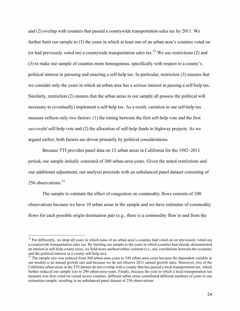
24
and (2) overlap with counties that passed a countywide transportation sales tax by 2011. We
further limit our sample to (3) the years in which at least one of an urban area’s counties voted on
(or had previously voted on) a countywide transportation sales tax.22 We use restrictions (2) and
(3) to make our sample of counties more homogenous, specifically with respect to a county’s
political interest in pursuing and enacting a self-help tax. In particular, restriction (3) ensures that
we consider only the years in which an urban area has a serious interest in passing a self-help tax.
Similarly, restriction (2) ensures that the urban areas in our sample all possess the political will
necessary to (eventually) implement a self-help tax. As a result, variation in our self-help tax
measure reflects only two factors: (1) the timing between the first self-help vote and the first
successful self-help vote and (2) the allocation of self-help funds to highway projects. As we
argued earlier, both factors are driven primarily by political considerations.
Because TTI provides panel data on 12 urban areas in California for the 1982–2011
period, our sample initially consisted of 360 urban-area-years. Given the noted restrictions and
one additional adjustment, our analysis proceeds with an unbalanced panel dataset consisting of
256 observations.23
The sample to estimate the effect of congestion on commodity flows consists of 100
observations because we have 10 urban areas in the sample and we have estimates of commodity
flows for each possible origin-destination pair (e.g., there is a commodity flow to and from the
22 Put differently, we drop all years in which none of an urban area’s counties had voted on (or previously voted on) a countywide transportation sales tax. By limiting our sample to the years in which counties had already demonstrated an interest in self-help county taxes, we hold more unobservables constant (i.e., any correlations between the economy and the political interest in a county self-help tax). 23 The sample size was reduced from 360 urban-area-years to 348 urban-area-years because the dependent variable in our models is an annual growth rate and because we do not observe 2011 annual growth rates. Moreover, two of the California urban areas in the TTI dataset do not overlap with a county that has passed a local transportation tax, which further reduced our sample size to 290 urban-area-years. Finally, because the year in which a local transportation tax measure was first voted on varied across counties, different urban areas contributed different numbers of years to our estimation sample, resulting in an unbalanced panel dataset of 256 observations.
25
Fresno urban area; there is also a commodity flow from Fresno to Riverside and from Riverside
to Fresno).
Table 2. Summary Statistics
Panel1:GDP,employment,andlaborearningsmodels Average Minimum MaximumAnnualgrowthrates(%)
a
UrbanareaGDP(%) 5.6 −9.3 18.0
Urbanareaemployment(%) 1.3 −9.8 6.8
Urbanarealaborearnings(%) 5.3 −14.7 30.%
Annualhoursofdelayperautocommuterb
34 2 89
Annualpercentageofsalestaxbaseallocatedtoself-helphighway
projects(%)c 0.2 0.0 0.5
Cumulativepercentageofsalestaxbaseallocatedtoself-help
highwayprojects(%)c 2.3 0.0 8.4
Urbanareapopulation(thousands)b
2,628 175 13,124
Panel2:Commodityflowmodel 2007–2010inter-urban-areacommodityflowgrowthrate(%)
d −36 −61 73
Annualhoursofdelayperautocommuterin2007b 41.40 14.00 86.00
Cumulativepercentageofsalestaxbaseallocatedtoself-help
highwayprojectsin2007(%)c
3.9 0.0 7.9
Urbanareapopulationin2007(thousands)b 2,729 390 12,800
Sources: a Emilia Istrate, Alan Berube, and Carey Anne Nadeau (2012), “Global MetroMonitor 2011: Volatility, Growth, and Recovery,” Report, Brookings Institution, Washington, DC; b Texas Transportation Institute; c
California county websites; Amber E. Crabbe et al. (2005), “Local Transportation Sales Taxes: California’s Experiment in Transportation Finance,” Public Budgeting & Finance 25 (3): 91–121; d California Statewide Freight Forecasting Model.
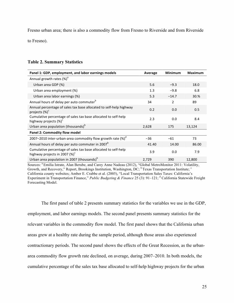
The first panel of table 2 presents summary statistics for the variables we use in the GDP,
employment, and labor earnings models. The second panel presents summary statistics for the
relevant variables in the commodity flow model. The first panel shows that the California urban
areas grew at a healthy rate during the sample period, although those areas also experienced
contractionary periods. The second panel shows the effects of the Great Recession, as the urban-
area commodity flow growth rate declined, on average, during 2007–2010. In both models, the
cumulative percentage of the sales tax base allocated to self-help highway projects for the urban
26
areas in our sample, which is affected by when an urban area first voted on a self-help tax, is
small—less than 9 percent.
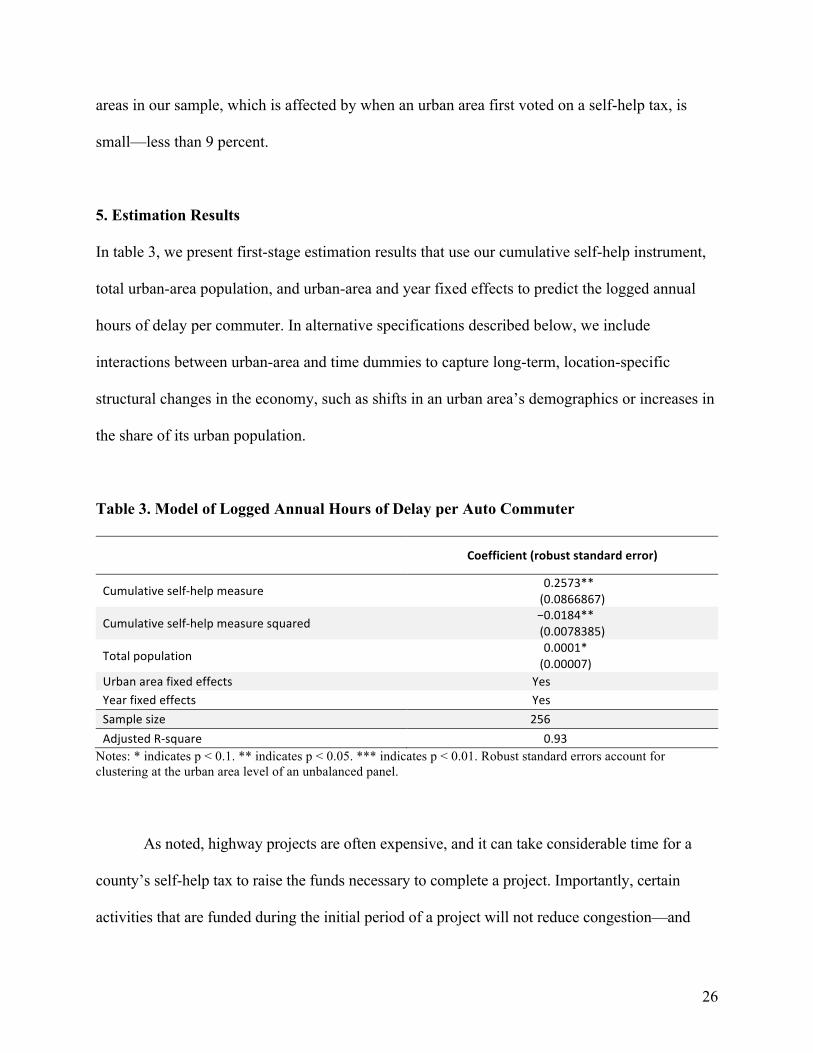
5. Estimation Results
In table 3, we present first-stage estimation results that use our cumulative self-help instrument,
total urban-area population, and urban-area and year fixed effects to predict the logged annual
hours of delay per commuter. In alternative specifications described below, we include
interactions between urban-area and time dummies to capture long-term, location-specific
structural changes in the economy, such as shifts in an urban area’s demographics or increases in
the share of its urban population.
Table 3. Model of Logged Annual Hours of Delay per Auto Commuter
Coefficient(robuststandarderror)
Cumulativeself-helpmeasure0.2573**
(0.0866867)
Cumulativeself-helpmeasuresquared−0.0184**
(0.0078385)
Totalpopulation0.0001*
(0.00007)
Urbanareafixedeffects Yes
Yearfixedeffects Yes
Samplesize 256
AdjustedR-square 0.93
Notes: * indicates p < 0.1. ** indicates p < 0.05. *** indicates p < 0.01. Robust standard errors account for clustering at the urban area level of an unbalanced panel.
As noted, highway projects are often expensive, and it can take considerable time for a
county’s self-help tax to raise the funds necessary to complete a project. Importantly, certain
activities that are funded during the initial period of a project will not reduce congestion—and
27
some may increase it. The most important activities include engineering analyses that California
may require before actual roadwork begins to satisfy environmental and safety regulations and the
formation of work zones. A work zone is an area of a highway where construction, maintenance,
or utility work activities occur, and it is typically marked by signs (especially ones that indicate
reduced speed limits), traffic-channeling devices, barriers, and work vehicles. The FHA estimates
that work zones accounted for nearly 900 million person-hours of delay in 2014.24
We specify a linear term and a squared term for the cumulative self-help measure to
capture the effect of highway spending on annual delay as it evolves. The estimates of both
coefficients are statistically significant. The positive coefficient for the linear term suggests that
additional self-help tax revenue is associated with greater delay in the short run, as would be
expected when work zones are formed at the beginning of a project. The negative coefficient for
the squared term suggests that additional self-help tax revenue is associated with less delay in the
long run as projects are completed, thereby increasing road capacity and improving road quality
to facilitate higher speeds.25
It is useful to provide more perspective on those results. Using the estimated coefficients,
we find that congestion levels begin to fall once the cumulative share of the local sales tax base
that is spent on self-help-tax highway projects is roughly 7 percent.26 The time it takes a county
to reach that cumulative share depends on the share of the tax base that a county dedicates to
self-help tax highway projects each year. For example, if a county (1) has an annual self-help tax
24 See Work Zone Management Program (2016). 25 It is possible that a self-help tax in a given county may have spillover effects that improve traffic flows between two counties that did not pass self-help taxes because traffic between those counties goes through the county that passed a self-help tax. However, we are unable to measure that effect with our data. 26 We obtain this result by calculating when highway congestion peaks—that is, by setting the derivative of our first-stage regression with respect to the cumulative percentage of self-help taxes spent on highways at zero and then solving for the cumulative percentage of self-help taxes spent on highways. We find that congestion peaked when the cumulative percentage of self-help taxes spent on highways reached 6.99 percent, after which congestion fell.
28
of 0.5 percent and (2) dedicates 100 percent of that tax to highway projects, holding all else
constant, congestion levels for the county would start decreasing 14 years after passing the self-
help tax [6.99% / (0.50% × 1.00)]. Put differently, for the first 14 years, all other things being
equal, more self-help highway expenditures cause more congestion; after 14 years, more
expenditures reduce congestion levels. As noted, depending on the project, some expenditures
may be used to pay for engineering analyses, which may take several years, or for maintenance
and construction in work zones, which cause congestion delays.
For the average county in our sample, the share of the annual self-help tax dedicated to
self-help highway projects is much less than 100 percent—roughly 34 percent;27 thus, because
the rate of revenue accumulation is so slow, it takes roughly 40 years before congestion levels
decline. In other words, only some counties in our sample accumulated self-help highway tax
revenue fast enough to cause congestion levels to fall in less than a few decades.
But this characterization of our findings should be strongly qualified because self-help
tax revenue is likely to be only one source of funding for an expensive and time-consuming
highway project that also receives state and federal funds. Indeed, as noted, the most common
prioritization criterion for projects funded by county self-help taxes is the ability to leverage state
and federal funding sources. Thus, we isolate the contribution of self-help tax revenue to
reducing congestion and imply that governent expenditures on highways do not reduce
congestion until decades after spending begins, which is inconsistent with research that finds that
such spending in metropolitan areas nationwide contemporaneously reduces congestion
(Winston and Langer 2006; Duranton and Turner 2011; Leduc and Wilson 2013).
27 Note, again, that this 34 percent corresponds to the average share of the self-help funds going to highway projects. A much smaller share of the local sales tax base goes to self-help highway projects, as shown in table 2.
29
Thus, an alternative—and possibly more accurate—explanation for our inverse-U
relationship between congestion and self-help expenditures is that the amount of self-help
highway spending is what matters for congestion, not the length of time since a self-help tax
measure was passed. For example, suppose that a county spends only very small amounts of its
self-help tax revenue on very small highway improvement projects, such as repainting highway
lines. Those marginal highway projects would probably increase congestion when they were
being implemented because lanes would need to be shut down. However, we would not expect
small projects on their own to have sizable long-run congestion-reducing effects. Thus, if a
county spent money on small projects for decades, we might expect cumulative revenue
spending to be positively associated with highway congestion. In other words, small highway
projects have all the negative side effects of increasing congestion in the short run and few
positive side effects of reducing congestion in the long run. At the same time, such projects could
be pursued because they also have safety, environmental, and other benefits.
In contrast, major and expensive highway projects (such as reconstructing or adding
highway lanes) raise congestion levels in the short run but ultimately reduce congestion in the
long run. But those projects are extremely expensive, and they are likely to be funded only if
county self-help tax revenue is combined with funding from the state and federal governments.
For example, the previously noted Sacramento County list of proposed projects includes a $700
million plan to widen the freeway from midtown to its junction with another freeway, but the
project could proceed only if self-help tax revenue were supplemented with state and federal
funds. Thus, according to this interpretation of our findings, when counties spend their self-help
tax revenue on big projects that also receive state and federal funding, they experience more
immediate reductions in congestion. When counties spend money on lots of small projects, they
30
do not achieve immediate reductions in congestion; in fact, they may increase congestion levels
for extended periods.
Because we do not have data on each county’s self-help tax revenue expenditures for
specific transportation projects, it is difficult to conclude whether our findings reflect the effect
of the passage of time or whether they result from the types of projects the counties chose to fund
over time. Although we explored alternative specifications that might capture those
considerations more fully than the preceding model did, none of them led to improvements in
explaining how county self-help taxes affect congestion.28 In any case, our first-stage estimation
results indicate that our instrument is strongly correlated with congestion (adjusted R2 = 0.93)
and that its economic effects are plausible.
5.1. Congestion’s Effects on Economic Performance Measures
We use the first-stage estimates to instrument annual delay and estimate its causal effect on the
economic performance measures. We specify log-linear functional forms for each specification
to present elasticities, and we control for both urban-area and year fixed effects, as well as for a
time-varying measure of urban-area population size. Although there is some concern that
populations may migrate in response to urban-area factors that affect both economic
performance and congestion levels, we suspect that such correlations are small, especially net of
the urban-area and year fixed effects. This hypothesis is supported by the fact that we do not
28 For example, we explored alternative specifications on the basis of discrete changes and lags in county self-help tax expenditures. Generally, those alternative measures of self-help tax revenue spending were not significantly correlated with congestion levels. However, when we (1) simply counted the number of years since an urban area began dedicating self-help tax funds toward highway projects and (2) used that variable and its square as instruments in the regression, we found an inverse-U-shaped relationship between congestion and the years since an urban area began spending self-help tax revenue on highways. Under this specification, we also obtained roughly the same 2SLS results, discussed below, that we obtained with the cumulative revenue measures.
31
find that the estimated congestion effects change noticeably when we exclude population size
from the model.
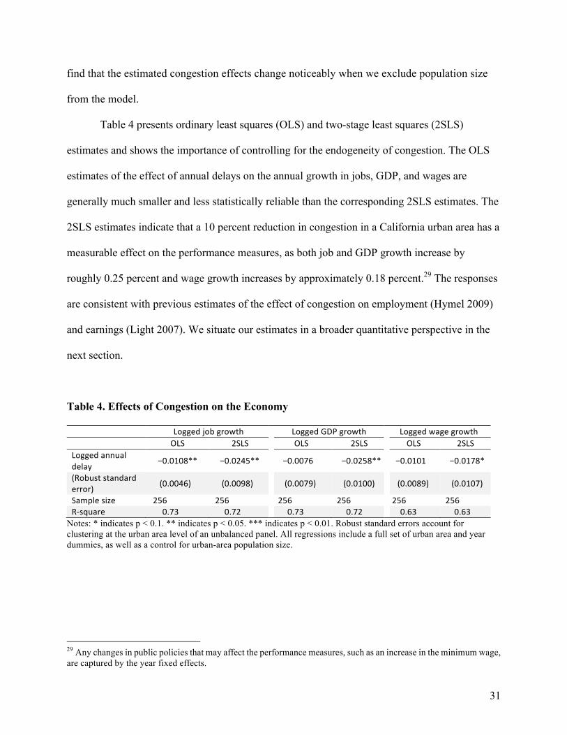
Table 4 presents ordinary least squares (OLS) and two-stage least squares (2SLS)
estimates and shows the importance of controlling for the endogeneity of congestion. The OLS
estimates of the effect of annual delays on the annual growth in jobs, GDP, and wages are
generally much smaller and less statistically reliable than the corresponding 2SLS estimates. The
2SLS estimates indicate that a 10 percent reduction in congestion in a California urban area has a
measurable effect on the performance measures, as both job and GDP growth increase by
roughly 0.25 percent and wage growth increases by approximately 0.18 percent.29 The responses
are consistent with previous estimates of the effect of congestion on employment (Hymel 2009)
and earnings (Light 2007). We situate our estimates in a broader quantitative perspective in the
next section.
Table 4. Effects of Congestion on the Economy
Loggedjobgrowth LoggedGDPgrowth Loggedwagegrowth
OLS 2SLS OLS 2SLS OLS 2SLS
Loggedannual
delay−0.0108** −0.0245** −0.0076 −0.0258** −0.0101 −0.0178*
(Robuststandard
error)(0.0046) (0.0098) (0.0079) (0.0100) (0.0089) (0.0107)
Samplesize 256 256 256 256 256 256
R-square 0.73 0.72 0.73 0.72 0.63 0.63
Notes: * indicates p < 0.1. ** indicates p < 0.05. *** indicates p < 0.01. Robust standard errors account for clustering at the urban area level of an unbalanced panel. All regressions include a full set of urban area and year dummies, as well as a control for urban-area population size.
29 Any changes in public policies that may affect the performance measures, such as an increase in the minimum wage, are captured by the year fixed effects.
32
For sensitivity analysis, we expand our controls in both stages to include interaction terms
between urban areas and decades (1980–1989, 1990–1999, 2000–2009, 2010–2012) to control for
any longer-term structural shifts that might have occurred in specific urban areas, such as changes
in population demographics. Not surprisingly, we find that the addition of those interaction terms
reduces the precision of our estimates of the congestion effects because they add some 30
parameters to the specification, although they still have some statistical significance; however, the
magnitudes of the estimated congestion effects also tend to increase. We also conduct two other
time-related sensitivity tests and find that the estimated congestion effects are robust.30 Finally,
we test the sensitivity of our job and wage growth models, which are based on county-level data
that were transformed to urban-area data, with models based on MSA-level data that were
transformed to urban-area data. We find only slightly smaller changes in the magnitude and
statistical reliability of our estimated congestion effects on job and wage growth.31
5.2. Congestion’s Effect on Commodity Freight Flows
As noted, we construct a measure of the three-year urban area growth rate of freight traffic
transported by truck across California counties. Because commodity traffic could be affected by
30 First, the start dates for self-help taxes seem to be in either the 1984–1990 or the 2004–2008 time frame, both of which include strong periods of growth. Thus, we replace the year dummies with a single time dummy where 1 indicates a year in the (1984–1990, 2004–2008) time frame and 0 otherwise; we interact this time dummy with the urban-area dummies. Thus, our model controls for urban-area-specific average growth rates across the years (1984–1990, 2004–2008). Under this new specification, the congestion effects become stronger, if anything, and retain their statistical significance. Second, we include interactions between the urban-area dummies and an indicator for the (2007, 2008) time period to capture urban-area-specific effects of the Great Recession. We also include individual-year dummies for 2007 and 2008. The congestion effects generally remain economically and statistically significant for this specification. However, it is likely that different urban areas may have been affected at different times and for different time periods by the Great Recession, but we have no systematic way of specifying time dummies and interacting them with the urban-area dummies to capture that possibility. 31 The full set of parameter estimates for the models used for sensitivity analysis is available on request from the authors.
33
congestion at the urban area of both its origin and destination, we instrument origin and
destination congestion with each urban area’s cumulative self-help highway tax revenue.
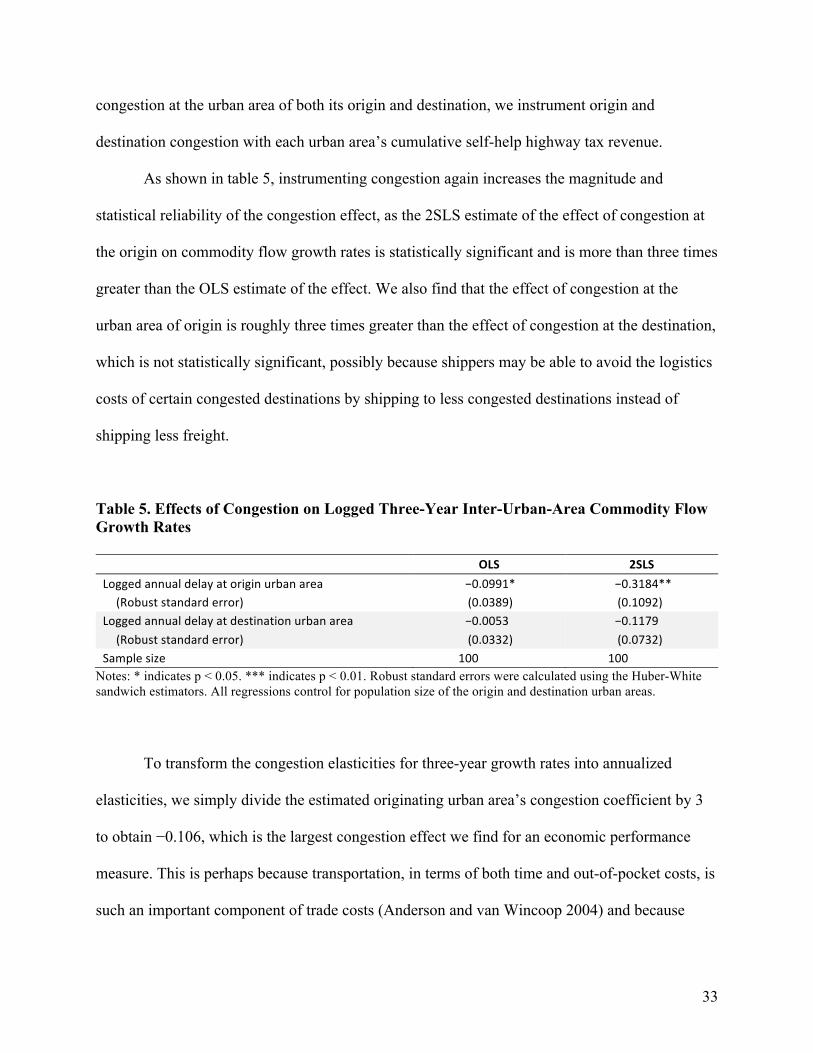
As shown in table 5, instrumenting congestion again increases the magnitude and
statistical reliability of the congestion effect, as the 2SLS estimate of the effect of congestion at
the origin on commodity flow growth rates is statistically significant and is more than three times
greater than the OLS estimate of the effect. We also find that the effect of congestion at the
urban area of origin is roughly three times greater than the effect of congestion at the destination,
which is not statistically significant, possibly because shippers may be able to avoid the logistics
costs of certain congested destinations by shipping to less congested destinations instead of
shipping less freight.
Table 5. Effects of Congestion on Logged Three-Year Inter-Urban-Area Commodity Flow Growth Rates OLS 2SLSLoggedannualdelayatoriginurbanarea −0.0991* −0.3184**
(Robuststandarderror) (0.0389) (0.1092)
Loggedannualdelayatdestinationurbanarea −0.0053 −0.1179
(Robuststandarderror) (0.0332) (0.0732)
Samplesize 100 100
Notes: * indicates p < 0.05. *** indicates p < 0.01. Robust standard errors were calculated using the Huber-White sandwich estimators. All regressions control for population size of the origin and destination urban areas.
To transform the congestion elasticities for three-year growth rates into annualized
elasticities, we simply divide the estimated originating urban area’s congestion coefficient by 3
to obtain −0.106, which is the largest congestion effect we find for an economic performance
measure. This is perhaps because transportation, in terms of both time and out-of-pocket costs, is
such an important component of trade costs (Anderson and van Wincoop 2004) and because
34
increases in transportation costs that are reflected in higher prices may cause receivers to obtain
freight from alternative points of origin.
For a sensitivity analysis of the commodity-flow growth model, we include the distance
between origin and destination urban areas, and characteristics of the origin and destination
urban areas in 2007, such as (1) the number of four-year colleges, (2) percentages of the
populations that were African American, and (3) percentages of the populations that were of
working age (20–64). Our results are largely robust to the inclusion of these controls.32
5.3. Further Comments on Identification
We find that the magnitude of OLS estimates of the effect of highway congestion on the
economic performance measures is consistently smaller than the magnitude of the 2SLS
estimates of that effect. Does the relative magnitude of the OLS and 2SLS estimates suggest that
our instrument is controlling for the relevant unobserved variables that could cause biased and
inconsistent estimates? Consider the OLS estimate of the effect of highway congestion on GDP
growth. Congestion is pro-cyclical because it generally increases with more economic activity.
Thus, unobserved variables that increase GDP growth are also likely to increase highway
congestion, and this positive correlation would create a bias that reduces the negative effect of
congestion on GDP growth. We argue that our instrumental variable purges the bias in the OLS
coefficient and that this results empirically in a larger negative coefficient, as shown in table 4.
Of course, there may be unobserved variables that have a negative effect on GDP. But are
any of those variables also likely to have a positive effect on highway congestion, which would
result in a negative correlation and an upward bias in the OLS estimates? If so, it is useful to
32 The full set of parameter estimates for the models is available on request from the authors.
35
consider whether our model controls for those unobservables, which could lead to biased
estimates. The most likely examples of those variables are natural events such as the October
1989 Loma Prieta earthquake, which caused a major section of the Oakland Bay Bridge to
collapse, disrupting economic activity throughout the Bay Area and increasing congestion
delays.33 However, natural events can be captured as random time-trend effects; thus, as a
robustness check, we reestimate our GDP, job, and wage growth models using a specification
that controls for those effects.
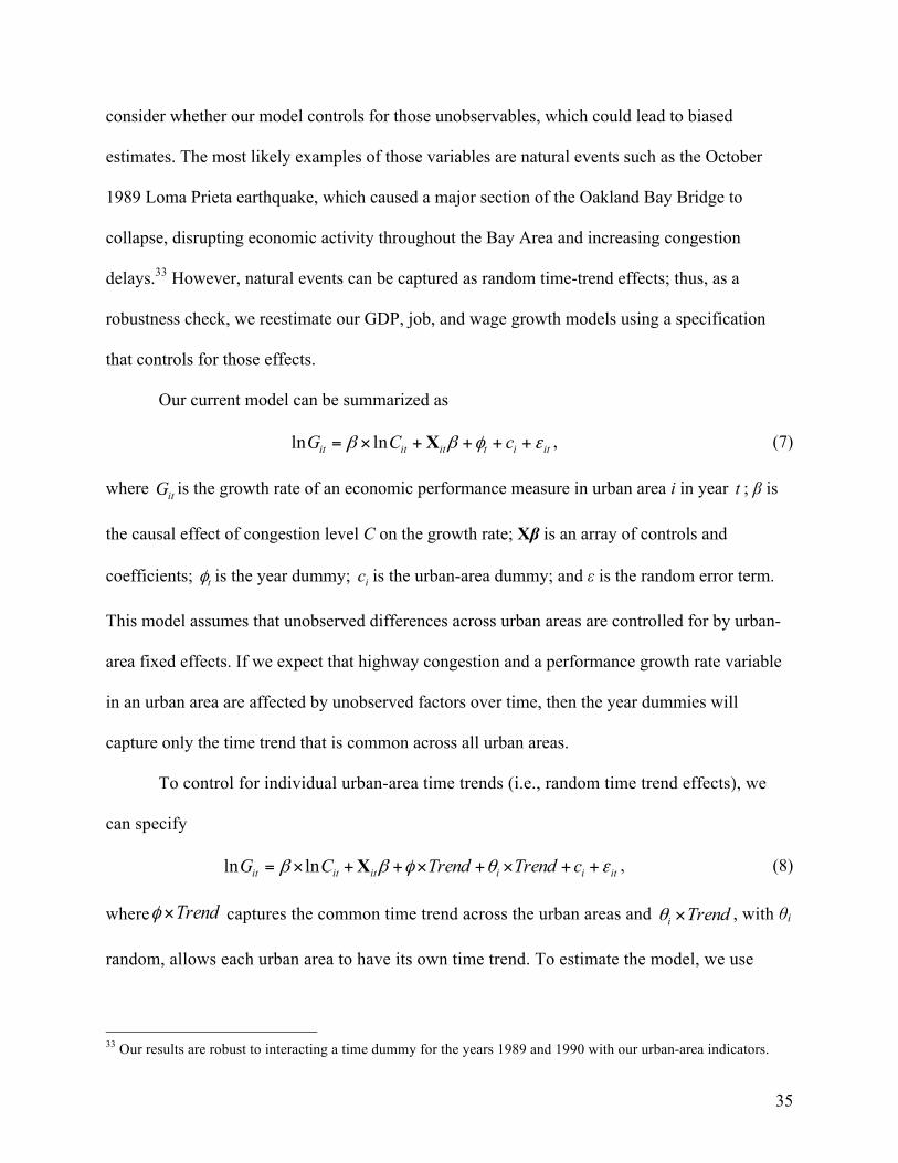
Our current model can be summarized as
, (7)
where is the growth rate of an economic performance measure in urban area i in year ; β is
the causal effect of congestion level C on the growth rate; Xβ is an array of controls and
coefficients; is the year dummy; is the urban-area dummy; and ε is the random error term.
This model assumes that unobserved differences across urban areas are controlled for by urban-
area fixed effects. If we expect that highway congestion and a performance growth rate variable
in an urban area are affected by unobserved factors over time, then the year dummies will
capture only the time trend that is common across all urban areas.
To control for individual urban-area time trends (i.e., random time trend effects), we
can specify
, (8)
where captures the common time trend across the urban areas and , with θi
random, allows each urban area to have its own time trend. To estimate the model, we use
33 Our results are robust to interacting a time dummy for the years 1989 and 1990 with our urban-area indicators.
ititititit cCG εφββ ++++×= Xlnln
itG t
tφ ic
itiiititit cTrendTrendCG εθφββ ++×+×++×= Xlnln
Trend×φ Trendi ×θ
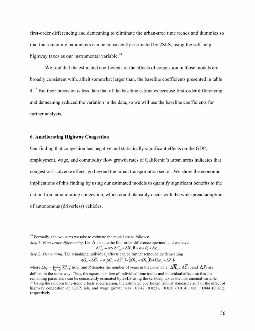
36
first-order differencing and demeaning to eliminate the urban-area time trends and dummies so
that the remaining parameters can be consistently estimated by 2SLS, using the self-help
highway taxes as our instrumental variable.34
We find that the estimated coefficients of the effects of congestion in those models are
broadly consistent with, albeit somewhat larger than, the baseline coefficients presented in table
4.35 But their precision is less than that of the baseline estimates because first-order differencing
and demeaning reduced the variation in the data, so we will use the baseline coefficients for
further analysis.
6. Ameliorating Highway Congestion
Our finding that congestion has negative and statistically significant effects on the GDP,
employment, wage, and commodity flow growth rates of California’s urban areas indicates that
congestion’s adverse effects go beyond the urban transportation sector. We show the economic
implications of this finding by using our estimated models to quantify significant benefits to the
nation from ameliorating congestion, which could plausibly occur with the widespread adoption
of autonomous (driverless) vehicles.
34 Formally, the two steps we take to estimate the model are as follows: Step 1: First-order differencing. Let denote the first-order difference operator, and we have
. Step 2: Demeaning. The remaining individual effects can be further removed by demeaning
,
where ∆cd = [;
fg;] ∆c12
fg;2:; and R denotes the number of years in the panel data. , , and are
defined in the same way. Thus, the equation is free of individual time trends and individual effects so that the remaining parameters can be consistently estimated by 2SLS using the self-help tax as the instrumental variable. 35 Using the random time-trend effects specification, the estimated coefficient (robust standard error) of the effect of highway congestion on GDP, job, and wage growth was −0.047 (0.025), −0.020 (0.014), and −0.044 (0.027), respectively.
Δitiititit CG εθφα Δ+++Δ+Δ×=Δ BX
( ) ( ) ( )⋅⋅⋅⋅ Δ−Δ+Δ−Δ+Δ−Δ=Δ−Δ iitiitiitiit CCGG εεα BXX
⋅Δ iX ⋅Δ iC ⋅Δ iε
37
Policymakers have been pursuing a piecemeal combination of policies that seek to
increase transportation funding and highway spending instead of trying to develop an efficient
strategy to reduce highway congestion (Winston 2013). Some policies may have modest effects
on reducing delays, but none offer the potential to change the flow of traffic in ways that would
substantially reduce congestion.36 That desired effect could be achieved by (1) efficient
congestion pricing, (2) technological advancements that make widespread use of autonomous
vehicles a reality in the coming years, and (3) a combination of (1) and (2).
Other assessments of congestion pricing focus on the benefits to motorists in travel time
savings and to the government in an improved highway budget balance that result from tolls that
could reduce delays by as much as 25 percent (Burris 2003, Calfee and Winston 1998). But does
it follow that such reductions in delays would also increase the growth rates of employment and
other economic performance measures? In the standard model (Walters 1961), congestion
pricing increases the cost of commuting to work during rush hour; thus, it reduces employment
unless the toll revenues are spent to reduce labor-inhibiting taxes (Parry and Bento 2001, Van
Dender 2003).
A general equilibrium model with motorists who have heterogeneous values of time and
reliability would consider the labor supply decisions of workers and the hiring decisions of firms.
By reducing travel time and improving reliability, congestion pricing could enable workers to
expand their area of job search, improve matching, and strengthen job retention. Employment
could therefore increase because the improved travel conditions would likely benefit people who
place a high value on travel time and commuting reliability. Firms may find that they can reduce
36 Winston and Langer (2006) find that government highway spending, which includes money from the FHA’s Highway Trust Fund that is allocated to states based on formulas that account for the size of a state’s road system but not for the level of congestion in a state’s metropolitan areas, has a small effect on reducing the cost of delays to motorists, shippers, and truckers.
38
their inventories because congestion pricing reduces delays and unreliability, which would lower
costs and enable companies to produce more output and hire more people. However, we are not
aware of any evidence that confirms that congestion pricing would have such favorable effects.
Thus, we have no empirical basis for considering the effect of congestion pricing on California’s,
or the nation’s, economic performance, although we suggest that these potential effects merit
further research.
Autonomous vehicles represent a positive exogenous technological shock that
transportation engineers conclude would significantly reduce congestion and delays by
improving traffic flows and reducing accidents. For example, Fagnant and Kockelman (2013)
provide empirical estimates that suggest highway congestion could potentially be reduced 50
percent with a 50 percent market penetration of autonomous vehicles, even accounting for the
additional travel autonomous vehicles would induce (Downs 1962).37 Reductions in delays could
have direct positive effects on the growth rates of economic performance measures. In fact, some
of the effects might be larger than we can account for here. For example, Smart and Klein (2015)
find that carless households can raise their incomes if they have access to a car but that the cost
of a new or used car is generally higher than the income gain. However, driverless cars, which
could be owned or hired at a lower cost than regular cars because their insurance costs would be
much lower, among other factors, would be readily available to any traveler and therefore
provide additional benefits by increasing employment and earnings for carless households.
37 Fagnant and Kockelman (2013) draw on several studies and highway engineering considerations to quantify the effects of autonomous vehicles on congestion, including smoothed traffic flow and bottleneck reductions, fewer crashes and incident delays, better routing choices, and further capacity enhancements. These authors acknowledge and account for the possibility that such improvements could be offset to some extent by additional travel induced by autonomous vehicles. The actual effect of autonomous vehicles on congestion could, of course, be greater or smaller than the effect we assume here; nonetheless, a 50 percent market penetration would significantly reduce congestion, and more importantly, congestion would continue to decline as autonomous vehicles’ penetration rate increased.
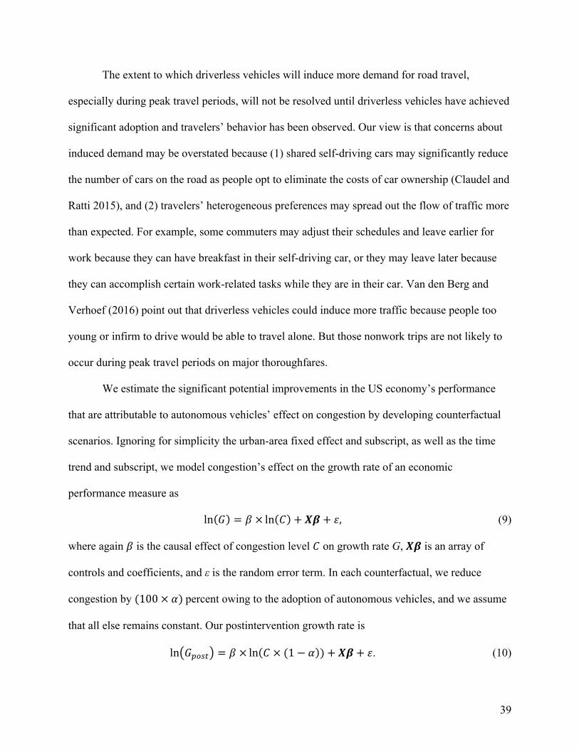
39
The extent to which driverless vehicles will induce more demand for road travel,
especially during peak travel periods, will not be resolved until driverless vehicles have achieved
significant adoption and travelers’ behavior has been observed. Our view is that concerns about
induced demand may be overstated because (1) shared self-driving cars may significantly reduce
the number of cars on the road as people opt to eliminate the costs of car ownership (Claudel and
Ratti 2015), and (2) travelers’ heterogeneous preferences may spread out the flow of traffic more
than expected. For example, some commuters may adjust their schedules and leave earlier for
work because they can have breakfast in their self-driving car, or they may leave later because
they can accomplish certain work-related tasks while they are in their car. Van den Berg and
Verhoef (2016) point out that driverless vehicles could induce more traffic because people too
young or infirm to drive would be able to travel alone. But those nonwork trips are not likely to
occur during peak travel periods on major thoroughfares.
We estimate the significant potential improvements in the US economy’s performance
that are attributable to autonomous vehicles’ effect on congestion by developing counterfactual
scenarios. Ignoring for simplicity the urban-area fixed effect and subscript, as well as the time
trend and subscript, we model congestion’s effect on the growth rate of an economic
performance measure as
ln c = k× ln m + op + q, (9)
where again k is the causal effect of congestion level m on growth rate G, op is an array of
controls and coefficients, and ε is the random error term. In each counterfactual, we reduce
congestion by (100×s)percent owing to the adoption of autonomous vehicles, and we assume
that all else remains constant. Our postintervention growth rate is
ln cuDB2 = k× ln m×(1 − s ) + op + q. (10)
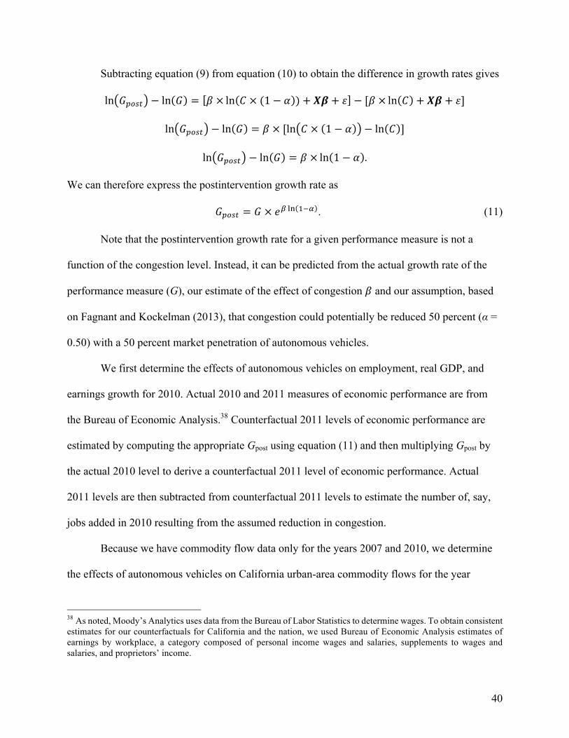
40
Subtracting equation (9) from equation (10) to obtain the difference in growth rates gives
ln cuDB2 − ln c = k× ln m×(1 − s ) + op + q − [k× ln m + op + q]
ln cuDB2 − ln c = k×[ln m× 1 − s − ln m ]
ln cuDB2 − ln c = k× ln 1 − s .
We can therefore express the postintervention growth rate as
cuDB2 = c×)w xy ;gz . (11)
Note that the postintervention growth rate for a given performance measure is not a
function of the congestion level. Instead, it can be predicted from the actual growth rate of the
performance measure (G), our estimate of the effect of congestion k and our assumption, based
on Fagnant and Kockelman (2013), that congestion could potentially be reduced 50 percent (α =
0.50) with a 50 percent market penetration of autonomous vehicles.
We first determine the effects of autonomous vehicles on employment, real GDP, and
earnings growth for 2010. Actual 2010 and 2011 measures of economic performance are from
the Bureau of Economic Analysis.38 Counterfactual 2011 levels of economic performance are
estimated by computing the appropriate Gpost using equation (11) and then multiplying Gpost by
the actual 2010 level to derive a counterfactual 2011 level of economic performance. Actual
2011 levels are then subtracted from counterfactual 2011 levels to estimate the number of, say,
jobs added in 2010 resulting from the assumed reduction in congestion.
Because we have commodity flow data only for the years 2007 and 2010, we determine
the effects of autonomous vehicles on California urban-area commodity flows for the year
38 As noted, Moody’s Analytics uses data from the Bureau of Labor Statistics to determine wages. To obtain consistent estimates for our counterfactuals for California and the nation, we used Bureau of Economic Analysis estimates of earnings by workplace, a category composed of personal income wages and salaries, supplements to wages and salaries, and proprietors’ income.
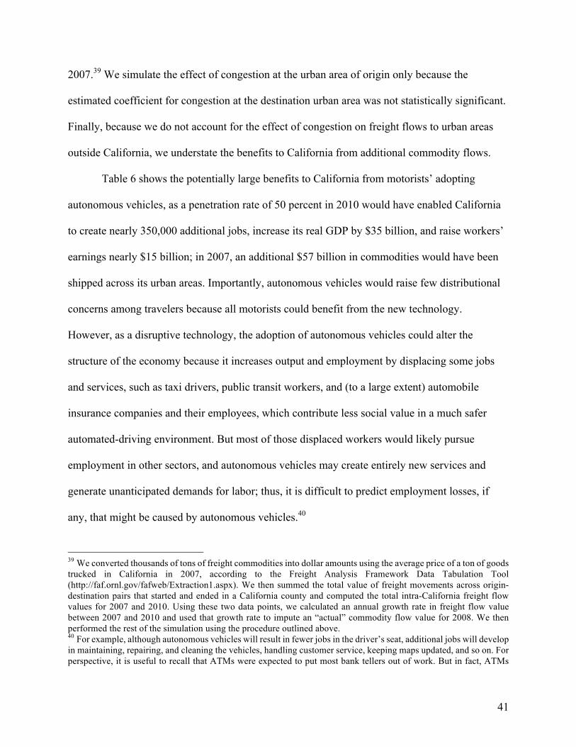
41
2007.39 We simulate the effect of congestion at the urban area of origin only because the
estimated coefficient for congestion at the destination urban area was not statistically significant.
Finally, because we do not account for the effect of congestion on freight flows to urban areas
outside California, we understate the benefits to California from additional commodity flows.
Table 6 shows the potentially large benefits to California from motorists’ adopting
autonomous vehicles, as a penetration rate of 50 percent in 2010 would have enabled California
to create nearly 350,000 additional jobs, increase its real GDP by $35 billion, and raise workers’
earnings nearly $15 billion; in 2007, an additional $57 billion in commodities would have been
shipped across its urban areas. Importantly, autonomous vehicles would raise few distributional
concerns among travelers because all motorists could benefit from the new technology.
However, as a disruptive technology, the adoption of autonomous vehicles could alter the
structure of the economy because it increases output and employment by displacing some jobs
and services, such as taxi drivers, public transit workers, and (to a large extent) automobile
insurance companies and their employees, which contribute less social value in a much safer
automated-driving environment. But most of those displaced workers would likely pursue
employment in other sectors, and autonomous vehicles may create entirely new services and
generate unanticipated demands for labor; thus, it is difficult to predict employment losses, if
any, that might be caused by autonomous vehicles.40
39 We converted thousands of tons of freight commodities into dollar amounts using the average price of a ton of goods trucked in California in 2007, according to the Freight Analysis Framework Data Tabulation Tool (http://faf.ornl.gov/fafweb/Extraction1.aspx). We then summed the total value of freight movements across origin-destination pairs that started and ended in a California county and computed the total intra-California freight flow values for 2007 and 2010. Using these two data points, we calculated an annual growth rate in freight flow value between 2007 and 2010 and used that growth rate to impute an “actual” commodity flow value for 2008. We then performed the rest of the simulation using the procedure outlined above. 40 For example, although autonomous vehicles will result in fewer jobs in the driver’s seat, additional jobs will develop in maintaining, repairing, and cleaning the vehicles, handling customer service, keeping maps updated, and so on. For perspective, it is useful to recall that ATMs were expected to put most bank tellers out of work. But in fact, ATMs
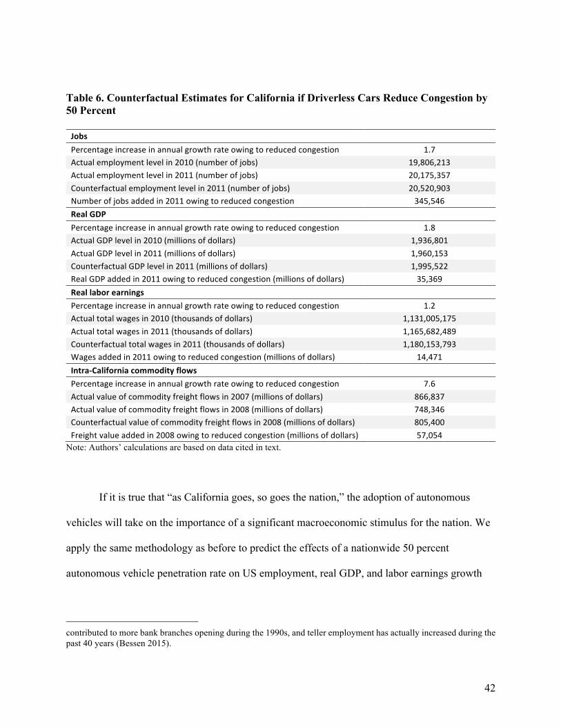
42
Table 6. Counterfactual Estimates for California if Driverless Cars Reduce Congestion by 50 Percent Jobs Percentageincreaseinannualgrowthrateowingtoreducedcongestion 1.7
Actualemploymentlevelin2010(numberofjobs) 19,806,213
Actualemploymentlevelin2011(numberofjobs) 20,175,357
Counterfactualemploymentlevelin2011(numberofjobs) 20,520,903
Numberofjobsaddedin2011owingtoreducedcongestion 345,546
RealGDP Percentageincreaseinannualgrowthrateowingtoreducedcongestion 1.8
ActualGDPlevelin2010(millionsofdollars) 1,936,801
ActualGDPlevelin2011(millionsofdollars) 1,960,153
CounterfactualGDPlevelin2011(millionsofdollars) 1,995,522
RealGDPaddedin2011owingtoreducedcongestion(millionsofdollars) 35,369
Reallaborearnings Percentageincreaseinannualgrowthrateowingtoreducedcongestion 1.2
Actualtotalwagesin2010(thousandsofdollars) 1,131,005,175
Actualtotalwagesin2011(thousandsofdollars) 1,165,682,489
Counterfactualtotalwagesin2011(thousandsofdollars) 1,180,153,793
Wagesaddedin2011owingtoreducedcongestion(millionsofdollars) 14,471
Intra-Californiacommodityflows Percentageincreaseinannualgrowthrateowingtoreducedcongestion 7.6
Actualvalueofcommodityfreightflowsin2007(millionsofdollars) 866,837
Actualvalueofcommodityfreightflowsin2008(millionsofdollars) 748,346
Counterfactualvalueofcommodityfreightflowsin2008(millionsofdollars) 805,400
Freightvalueaddedin2008owingtoreducedcongestion(millionsofdollars) 57,054
Note: Authors’ calculations are based on data cited in text.
If it is true that “as California goes, so goes the nation,” the adoption of autonomous
vehicles will take on the importance of a significant macroeconomic stimulus for the nation. We
apply the same methodology as before to predict the effects of a nationwide 50 percent
autonomous vehicle penetration rate on US employment, real GDP, and labor earnings growth
contributed to more bank branches opening during the 1990s, and teller employment has actually increased during the past 40 years (Bessen 2015).
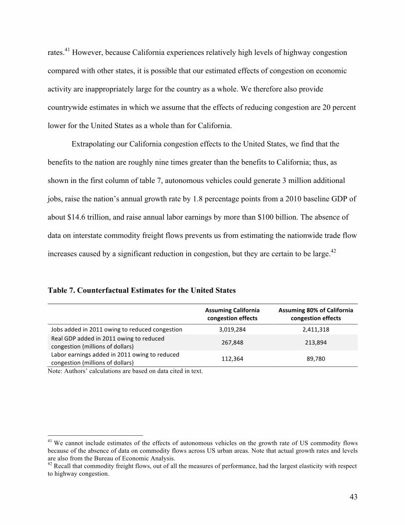
43
rates.41 However, because California experiences relatively high levels of highway congestion
compared with other states, it is possible that our estimated effects of congestion on economic
activity are inappropriately large for the country as a whole. We therefore also provide
countrywide estimates in which we assume that the effects of reducing congestion are 20 percent
lower for the United States as a whole than for California.
Extrapolating our California congestion effects to the United States, we find that the
benefits to the nation are roughly nine times greater than the benefits to California; thus, as
shown in the first column of table 7, autonomous vehicles could generate 3 million additional
jobs, raise the nation’s annual growth rate by 1.8 percentage points from a 2010 baseline GDP of
about $14.6 trillion, and raise annual labor earnings by more than $100 billion. The absence of
data on interstate commodity freight flows prevents us from estimating the nationwide trade flow
increases caused by a significant reduction in congestion, but they are certain to be large.42
Table 7. Counterfactual Estimates for the United States
AssumingCaliforniacongestioneffects
Assuming80%ofCaliforniacongestioneffects
Jobsaddedin2011owingtoreducedcongestion 3,019,284 2,411,318
RealGDPaddedin2011owingtoreduced
congestion(millionsofdollars)267,848 213,894
Laborearningsaddedin2011owingtoreduced
congestion(millionsofdollars)112,364 89,780
Note: Authors’ calculations are based on data cited in text.
41 We cannot include estimates of the effects of autonomous vehicles on the growth rate of US commodity flows because of the absence of data on commodity flows across US urban areas. Note that actual growth rates and levels are also from the Bureau of Economic Analysis. 42 Recall that commodity freight flows, out of all the measures of performance, had the largest elasticity with respect to highway congestion.
44
A disruptive technology that generates such a large stimulus would undoubtedly activate
various macroeconomic responses, including by the Federal Reserve; thus, the positive effects
might be transformed in various ways. For example, the workforce would gain from more wage
growth and less job growth if, in fact, the workforce were already fully employed and
immigration were further restricted.
If we assume that highway congestion reductions from autonomous vehicles in the
United States would have 80 percent of the economic boost that they would have in California,
the benefits of autonomous vehicles would still be strikingly large, as shown in the second
column of table 7.43 Moreover, if we account for the effect of autonomous vehicles on improving
the reliability of travel, the estimated macroeconomic stimulus would be even larger because
another cost of distance would be reduced. In summary, even if our methodology and
conservative 80 percent assumption lead us to inflate the magnitude of the national stimulus, our
omissions of other important potential benefits of autonomous vehicles undoubtedly lead us to
understate it on the whole.44
Policymakers could increase the efficiency of the nation’s highway system by combining
congestion pricing with the adoption of autonomous vehicles, and there is some congressional
43 Other countries’ economies also have the potential to benefit significantly from the adoption of autonomous vehicles. Gill et al. (2015) provide an overview of the benefits of autonomous vehicles for the Canadian economy. 44 Autonomous trucks would also benefit the national economy by improving the speed, reliability, and safety of transporting freight by truck and by addressing the shortage of truck drivers. Otto, Peloton, Volvo, and Daimler are among the companies developing and testing autonomous trucks. The adoption of autonomous trucks and automobiles would also reduce the amount of required parking space because the vehicles could be stored in remote parking garages. In addition, traffic would not be impeded by drivers cruising for parking places. The urban space that would become available could boost agglomeration economies. Autonomous vehicles are likely to lead to less stressful commutes, which would have significant benefits to health and productivity (“Health in a Hurry” 2016) and to many fewer traffic stops and potential confrontations with police. Finally, autonomous buses represent a potential improvement in public transit service and cost efficiency, which could also reduce the billions of dollars in taxpayer-funded subsidies.
45
support for this action.45 Although it is not clear how congestion pricing would affect the growth
rates of the performance measures, it would offset any increase in highway congestion caused by
increased demand for autonomous vehicles. Moreover, efficient road pricing would be more
politically palatable in the new driving environment because a notable percentage of people
would not own cars and would simply hire an autonomous vehicle when they needed
transportation. Hence, congestion tolls may be perceived as similar to paying a toll when using a
taxi and would be more likely to be accepted.
It may seem implausible that such improvements in highway travel—significant as they
are—could also have such large macroeconomic effects. However, the importance of
improvements in mobility to the development of the US economy has long been recognized. For
example, Krugman (2009) explains how this country’s railroads, by reducing transportation costs
and the costs of distance, facilitated large-scale production (economies of scale) and transformed
the US economy into a differentiated farm belt and manufacturing belt. To be sure, today’s
transportation system is much more advanced than the system that was in place when railroad
service became available in the 1800s; but highways affect a considerable amount of the nation’s
inputs (labor and capital) and outputs because they account for roughly 90 percent of urban
commuter travel, 70 percent of intercity passenger travel, and roughly 30 percent of intercity
freight traffic (Winston 2013).
45 For example, Representative Earl Blumenauer (2016), of Oregon’s Third Congressional District, argues that the data collection, reporting, and debiting that would be standard in autonomous vehicles could provide a payment platform that could be used to charge for driving during peak travel times.
46
7. Final Comments
Recent research has begun to explore how automobile commuting, especially in congested
conditions, can damage adults’ and infants’ physical and emotional health and well-being
(Fottrell 2015; Knittel, Miller, and Sanders 2016). Here, we take a broader perspective and
explore how congested highways affected the health of the California economy. As a potential
cure for sluggish economic growth, and as an example of a life-altering innovation that conflicts
with Gordon’s (2016) pessimistic view of the lack of future innovations that may improve living
standards, we suggest that the technological advance of autonomous vehicles could significantly
improve the nation’s GDP growth, employment, and labor earnings, especially because
autonomous vehicles would both increase consumption and save lives (Jones 2016).
We acknowledge that autonomous vehicles may reduce congestion less than we have
indicated here because the decreased time and operating costs of automobile travel may induce
people to take additional trips unless they face peak-period user charges. If so, the overall
benefits we estimate would not decline; instead, some would be reflected in the value of the
additional trips rather than in the benefits from less congestion.
In any case, microeconomic actions have rarely had such potentially important
macroeconomic effects. Moreover, unlike macroeconomic policies, the timing of those actions is
straightforward—sooner rather than later. Federal policymakers should facilitate this timing by
applying current vehicle regulations that allow manufacturers to self-certify compliance with
basic guidelines instead of allowing state and local officials to micromanage the public’s
adoption and use of autonomous vehicles; such micromanaging may stifle innovation.
47
References
Amiti, Mary, Tyler Bodine-Smith, Michele Cavallo, and Logan Lewis. 2015. “Did the West Coast Port Dispute Contribute to the First-Quarter GDP Slowdown?” Liberty Street Economics, Federal Reserve Bank of New York, July 2.
Anderson, James E., and Eric van Wincoop. 2004. “Trade Costs.” Journal of Economic
Literature 42 (3): 691–751. Angel, Shlomo, and Alejandro Blei. 2015. “Commuting and the Productivity of American Cities:
How Self-Adjusting Commuting Patterns Sustain the Productive Advantage of Larger Metropolitan Labor Markets.” New York University Marron Institute of Urban Management Working Paper No. 19, January 7.
Bessen, James. 2015. Learning by Doing: The Real Connection between Innovation, Wages, and
Wealth. New Haven, CT: Yale University Press. Bizjak, Tony. 2016. “Sacramento Unveils $3.6 Billion Transportation Project To-Do List.”
Sacramento Bee, March 27. Blumenauer, Earl. 2016. “Let’s Use Self-Driving Cars to Fix America’s Busted Infrastructure.”
Wired, May 20. Brown, Edmund G., Jr., Brian P. Kelly, and Malcolm Dougherty. 2014. “California Freight
Mobility Plan.” California State Transportation Agency, December. BLS (Bureau of Labor Statistics), US Department of Labor. 2016. “Quarterly Census of
Employment and Wages.” Accessed December 22. https://www.bls.gov/cew/. Burris, M. W. 2003. “The Toll-Price Component of Travel Demand Elasticity.” International
Journal of Transport Economics 30 (1): 45–59. Calfee, John, and Clifford Winston. 1998. “The Value of Automobile Travel Time: Implications
for Congestion Policy.” Journal of Public Economics 69 (1): 83–102. California Department of Transportation, Division of Transportation Planning, Economic
Analysis Branch. 2014. Transportation Funding in California: 2014. Sacramento, CA. Chetty, Raj, Nathaniel Hendren, Patrick Kline, and Emmanuel Saez. 2014. “Where Is the Land
of Opportunity? The Geography of Intergenerational Mobility in the United States.” NBER Working Paper No. 19843, National Bureau of Economic Analysis, Cambridge, MA.
Claudel, Matthew, and Carlo Ratti. 2015. “Full Speed Ahead: How the Driverless Car Could
Transform Cities.” McKinsey and Company, Washington, DC.
48
CPCS Transcom Inc. 2015. Unclogging America’s Arteries 2015: Prescriptions for Healthier Highways. Washington, DC: American Highway Users Alliance.
Crabbe, Amber E., Rachel Hiatt, Susan D. Poliwka, and Martin Wachs. 2005. “Local
Transportation Sales Taxes: California’s Experiment in Transportation Finance.” Public Budgeting & Finance 25 (3): 91–121.
Downs, Anthony. 1962. “The Law of Peak-Hour Expressway Congestion.” Traffic Quarterly 16
(3): 393–409. Duranton, Gilles, and Matthew A. Turner. 2011. “The Fundamental Law of Road Congestion:
Evidence from US Cities.” American Economic Review 101 (6): 2616–52. Fagnant, Daniel J., and Kara Kockelman. 2013. “Preparing a Nation for Autonomous Vehicles:
Opportunities, Barriers and Policy Recommendations for Capitalizing on Self-Driven Vehicles.” Preprint for Transportation Research Part A 77 (2015): 167–181.
FHA (Federal Highway Administration), US Department of Transportation. 2009. “National
Household Travel Survey.” Washington, DC. http://nhts.ornl.gov. ———. 2015. “Highway Performance Monitoring System (HPMS).” Office of Highway Policy
Information, Washington, DC. https://www.fhwa.dot.gov/policyinformation/hpms.cfm. ———. 2016. “Freight Analysis Framework.” Washington, DC.
http://www.ops.fhwa.dot.gov/freight/freight_analysis/faf/. Fottrell, Quentin. 2015. “5 Ways Commuting Ruins Your Life.” Market Watch, September 9. Gill, Vijay, Barrie Kirk, Paul Godsmark, and Brian Flemming. 2015. “Automated Vehicles: The
Coming of the Next Disruptive Technology.” Report, Conference Board of Canada, Ottawa.
Gordon, Robert J. 2016. The Rise and Fall of American Growth: The U.S. Standard of Living
since the Civil War. The Princeton Economic History of the Western World. Princeton, NJ: Princeton University Press.
Harrison, David, and Heather Gillers. 2016. “American Paradox: It’s Never Been Cheaper for
Cities and States to Borrow Money . . . and They Refuse to Do It.” Wall Street Journal, August 7.
“Health in a Hurry: The Impact of Rush Hour Commuting on Our Health and Wellbeing.” 2016.
London: Royal Society for Public Health. Hymel, Kent. 2009. “Does Traffic Congestion Reduce Employment Growth?” Journal of Urban
Economics 65 (2): 127–35.
49
Istrate, Emilia, Alan Berube, and Carey Anne Nadeau. 2012. “Global MetroMonitor 2011: Volatility, Growth, and Recovery.” Report, Brookings Institution, Washington, DC.
Istrate, Emilia, Anya Nowakowski, and Kavita Mak. 2014. “The Road Ahead: County
Transportation Funding and Financing.” NACo Policy Research Paper Series Issue 2, National Association of Counties, Washington, DC.
Jones, Charles I. 2016. “Life and Growth.” Journal of Political Economy 124 (2): 539–78. Kalra, Nidhi, and Susan M. Paddock. 2016. “Driving to Safety: How Many Miles of Driving
Would It Take to Demonstrate Autonomous Vehicle Reliability?” Research Report No. RR-1478-RC, Rand Corporation, Santa Monica, CA.
Kitagawa, Toru. 2015. “A Test for Instrument Validity.” Econometrica 83 (5): 2043–63. Knittel, Christopher R., Douglas L. Miller, and Nicholas J. Sanders. 2016. “Caution, Drivers!
Children Present: Traffic, Pollution, and Infant Health.” Review of Economics and Statistics 98 (2): 350–66.
Krugman, Paul. 2009. “The Increasing Returns Revolution in Trade and Geography.” American
Economic Review 99 (3): 561–71. Langer, Ashley, Vikram Maheshri, and Clifford Winston. 2016. “From Gallons to Miles: A
Disaggregate Analysis of Automobile Travel and Externality Taxes.” Working paper. Langer, Ashley, and Clifford Winston. 2008. “Toward a Comprehensive Assessment of Road
Pricing Accounting for Land Use.” In Brookings-Wharton Papers on Urban Affairs 2008, edited by Gary Burtless and Janet Rothenberg Pack, 127–75. Washington, DC: Brookings Institution.
Leduc, Sylvain, and Daniel Wilson. 2013. “Roads to Prosperity or Bridges to Nowhere? Theory
and Evidence on the Impact of Public Infrastructure Investment.” In NBER Macroeconomics Annual 2012, volume 27, edited by Daron Acemoglu, Jonathan Parker, and Michael Woodford, 89–142. Chicago: University of Chicago Press.
Li, Shanjun, Joshua Linn, and Erich Muehlegger. 2014. “Gasoline Taxes and Consumer
Behavior.” American Economic Journal: Economic Policy 6 (4): 302–42. Light, Thomas. 2007. “Time-Use Approach for Estimating Commuters’ Value of Travel Time.”
Presented at Transportation Research Board 86th Annual Meeting, January 21–25, Washington, DC.
Lindsey, Robin. 2006. “Do Economists Reach a Conclusion on Road Pricing? The Intellectual
History of an Idea.” Econ Journal Watch 3 (2): 292–379.
50
Parry, Ian W. H., and Antonio Bento. 2001. “Revenue Recycling and the Welfare Effects of Road Pricing.” Scandinavian Journal of Economics 103 (4): 645–71.
Prud’homme, Remy, and Chang-Woon Lee. 1999. “Size, Sprawl, Speed and the Efficiency of
Cities.” Urban Studies 36 (1): 1849–58. Puga, Diego. 2010. “The Magnitude and Causes of Agglomeration Economies.” Journal of
Regional Science 50 (1): 203–19. Ranaiefar, F. 2014. “A Structural Direct Demand Model for Inter-Regional Commodity Flow
Forecasting.” PhD diss., Department of Civil Engineering, University of California, Irvine.
Ranaiefar, Fatemeh, Joseph Y. J. Chow, Daniel Rodriguez-Roman, Pedro V. Camargo, and
Stephen G. Ritchie. 2012. “Geographic Scalability and Supply Chain Elasticity of a Structural Commodity Generation Model Using Public Data.” Transportation Research Record: Journal of the Transportation Research Board 2378: 73–83.
Schrank, David, Bill Eisele, Tim Lomax, and Jim Bak. 2015. “2015 Urban Mobility Scorecard.”
Report, Texas A&M Transportation Institute, College Station, TX. Small, Kenneth A., Clifford Winston, and Carol A. Evans. 1989. Road Work: A New Highway
Pricing and Investment Policy. Washington, DC: Brookings Institution. Small, Kenneth A., Clifford Winston, and Jia Yan. 2005. “Uncovering the Distribution of
Motorists’ Preferences for Travel Time and Reliability.” Econometrica 73 (4): 1367–82. Smart, Michael J., and Nicholas J. Klein. 2015. “A Longitudinal Analysis of Cars, Transit, and
Employment Outcomes.” Report 12-49, Mineta National Transit Research Consortium, San Jose State University, San Jose, CA.
Sweet, Matthias. 2014. “Traffic Congestion’s Economic Impacts: Evidence from US
Metropolitan Regions.” Urban Studies 51 (10): 2088–2110. Van den Berg, Vincent A. C., and Erik T. Verhoef. 2016. “Robot Cars and Dynamic Bottleneck
Congestion: The Effects on Capacity, Value of Time and Preference Heterogeneity.” Discussion Paper TI 2015-062/VIII, Tinbergen Institute, Amsterdam.
Van Dender, Kurt. 2003. “Transport Taxes with Multiple Trip Purposes.” Scandinavian Journal
of Economics 105 (2): 295–310. Walters, A. A. 1961. “The Theory and Measurement of Private and Social Cost of Highway
Congestion.” Econometrica 29 (4): 676–99. Winston, Clifford. 2013. “On the Performance of the U.S. Transportation System: Caution
Ahead.” Journal of Economic Literature 51 (3): 773–824.
51
Winston, Clifford, and Ashley Langer. 2006. “The Effect of Government Highway Spending on
Road Users’ Congestion Costs.” Journal of Urban Economics 60 (3): 463–83. Winston, Clifford, and Fred L. Mannering. 2014. “Implementing Technology to Improve Public
Highway Performance: A Leapfrog Technology from the Private Sector Is Going to Be Necessary.” Economics of Transportation 3 (2): 158–65.
Work Zone Management Program. 2016. “Facts and Statistics—Work Zone Mobility.” Federal
Highway Administration, March 2. http://www.ops.fhwa.dot.gov/wz/resources/facts_stats/mobility.htm.


