Mon. Not. R. Astron. Soc. 350, 407–426 (2004) doi:10.1111/j.1365-2966.2004.07446.x

A new synthetic model for asymptotic giant branch stars

Robert G. Izzard,1� Christopher A. Tout,1 Amanda I. Karakas2,3 and Onno R. Pols4

1Institute of Astronomy, Madingley Road, Cambridge CB3 0HA2School of Mathematical Sciences, Monash University, Wellington Road, Clayton, Victoria 3800, Australia3Institute for Computational Astrophysics, Department of Astronomy & Physics, Saint Mary’s University, Halifax, NS B3H 3C3, Canada4Astronomical Institute Utrecht, Postbus 80000, 3508 TA Utrecht, the Netherlands

Accepted 2003 November 21. Received 2003 November 21; in original form 2003 January 23

ABSTRACTWe present a synthetic model for thermally pulsing asymptotic giant branch (TPAGB) evolutionconstructed by fitting expressions to full evolutionary models in the metallicity range 0.0001 �Z � 0.02. Our model includes parametrizations of third dredge-up and hot-bottom burning withmass and metallicity. The Large Magellanic Cloud and Small Magellanic Cloud carbon starluminosity functions are used to calibrate third dredge-up. We calculate yields appropriatefor galactic chemical evolution models for 1H, 4He, 12C, 13C, 14N, 15N, 16O and 17O. Theinitial–final mass relation is examined for our stars and found to fit to within 0.1 M� of theobservations. We also reproduce well the white dwarf mass function for masses above about0.58 M�. The new model is to be implemented in a rapid binary star evolution code.

Key words: stars: AGB and post-AGB – stars: carbon – ISM: abundances.

1 I N T RO D U C T I O N

Full stellar evolution models of thermally pulsing asymptotic giantbranch (TPAGB) stars are difficult and extremely time-consumingto make, and often suffer numerical failure. For this reason, syn-thetic models based on full stellar evolution models but with thecomplicated physics replaced by simple expressions are a usefulapproximation. Such models are well suited to exploring regions oflarge, multidimensional parameter spaces which would take yearsto explore with full stellar evolution models. Here we build on themodels of Groenewegen & de Jong (1993) and Wagenhuber &Groenewegen (1998) with accurate new parametrizations of thirddredge-up and hot-bottom burning (HBB), as well as new fits tostellar structure from our full stellar evolution models. Stellar evo-lution up to the TPAGB is handled by coupling the new code withthe rapid evolution code of Hurley, Pols & Tout (2000) and Hurley,Tout & Pols (2002, H02) which is designed for single, binary andstar cluster evolution. The eventual aim of this work is to implementTPAGB evolution and especially nucleosynthesis in the binary starmodel and, while this is yet some way off, we have made significantprogress in constructing a capable single star model. The calculationof binary star yields will result.

Table 1, mostly taken from the review of Henry (2004), sum-marizes attempts at calculating AGB yields to date. It does not in-clude important works on AGB evolution that do not specifically in-volve yield calculation, such as the series of works by Boothroyd &Sackmann (e.g. Boothroyd & Sackmann 1988) who investigateLi, Be, B and 12C/13C ratios in particular, Straniero et al. (1997)

�E-mail: rgi@ast.cam.ac.uk

who tackle the carbon star formation problem in low-mass (1 �M/M� � 3) solar-metallicity stars, Lattanzio and collaborators’contribution to HBB (Lattanzio et al. 1997), carbon star forma-tion (Lattanzio 1989) and degenerate pulses (Frost, Lattanzio &Wood 1998), Mowlavi and collaborators’ works on 26Al (Mowlavi& Meynet 2000), fluorine (Mowlavi, Jorissen & Arnould 1998) andsodium (Mowlavi 1999), and models by Herwig (2000) detailingconvective overshooting and its consequences. There are also count-less papers dealing specifically with the s-process in TPAGB stars(e.g. Busso et al. 2001).

Synthetic models have been constructed in the past (e.g. Renzini& Voli 1981; Iben & Renzini 1983) and are still very much in use(Mouhcine & Lancon 2003). Hybrid models which combine aspectsof synthetic and full evolution have also been constructed (Marigo,Bressan & Chiosi 1998; Marigo 1999, 2001). While we lean heavilyon the work of Groenewegen & de Jong (1993) and Wagenhuber &Groenewegen (1998), our new model has some marked differencesin its treatment of dredge-up and HBB. Most previous models as-sume a constant dredge-up parameter and minimum core mass fordredge-up. We include expressions fitted to our full stellar evolutionmodels (Karakas, Lattanzio & Pols 2002) for these and the stellarstructure (luminosity, radius, core mass, etc.). HBB is included in asimilar way to Groenewegen & de Jong (1993) but with calibrationof the free parameters to our full evolution models.

While the use of a purely synthetic code is inferior in accuracy ordetail to full stellar modelling [or the envelope burning technique ofMarigo 1999a (M99)], it is the only way to explore a large param-eter space such as a full study of binary stars. The single star spacecould conceivably consist of the mass M, metallicity Z and a fewfree parameters such as the minimum mass for dredge-up, dredge-upefficiency and perhaps the mass-loss rate. For binaries the problem

C© 2004 RAS

408 R. G. Izzard et al.

Table 1. Summary of existing TPAGB models. IT = Iben & Truran (1978); RV = Renzini & Voli (1981); HG = van den Hoek & Groenewegen (1997); FC =Forestini & Charbonnel (1997); M01 = Marigo (2001); C01 = Chieffi et al. (2001); K02 = Karakas et al. (2002); D03 = Dray et al. (2003). ‘Syn’ indicatesa synthetic TPAGB code; ‘SynEnv’ denotes a synthetic TPAGB code with envelope integration; ‘Full’ are full stellar evolution models covering the TPAGB.The HBB column contains ‘n’ = no, ‘a’ = analytic, and ‘net’ nuclear network (‘extrap’ is an extrapolation from full network calculations).

Authors Mass range (M�) Z range HBB Isotopes Model type Extras

IT 1–8 0.02 n 12,13C, 14N,22Ne SynRV 1–8 0.004–0.02 a 12,13C, 14N,16O SynHG 0.8–8 0.001–0.04 a 12,13C, 14N,16O SynFC 3–7 0.005-0.02 net/extrap many Syn/FullM01 0.8–6 0.004–0.019 net 12,13C, 14,15N,16,17,18O SynEnvC01 4–8 0 net many FullK02/D03 1–6(.5) 0.004 − 0.02 net many FullOur model 1–8 10−4–0.03 a 12,13C, 14,15N,16,17O,22Ne so far Syn Binaries

Table 2. List of variables.

Symbol Meaning

Z ZAMS metallicity (Z� = 0.02)M i ZAMS massM Instantaneous massMc Instantaneous core massMc,bagb Core mass at the base of the (E)AGBMc,1TP Core mass at the start of the TPAGBM1TP Mass at the start of the TPAGBMenv Envelope mass, calculated from M − Mc

Menv,1TP Envelope mass at the start of the TPAGBXi Mass fraction of isotope iM Stellar mass-loss rateζ log10(Z/0.02)

is worse, there are the two masses, separation and eccentricity,and in addition free parameters associated with uncertain detailsof common-envelope evolution, mass transfer and accretion and en-hanced wind loss owing to the companion. A parameter space takesa time δt × nN to explore, where δt is the average model time, n isthe number of grid-points per free parameter and N is the number offree parameters, so a fast model is desired. Our model has an averageexecution time (including features not described here, such as a com-panion star and associated mass transfer, NeNa and MgAl cycles,supernovae and novae) of 0.05 s on a 2.1-GHz AMD Athlon CPU1

(0.64 s on a Pentium Pro 200-MHz CPU2), so for a 106-point gridwe have a total execution time of nearly 14 h. An increase of δt to 1min (which would be an extremely fast full stellar evolution model)increases the total execution time to just less than 2 years.

The drawback of a fast code is a loss of accuracy and, while we tryto fit to our full evolution models as well as we can, it is impossibleto fit perfectly. We have to interpolate and sometimes extrapolateinto regions of parameter space where we cannot be sure that weget the correct answer. Since we aim to investigate binary stars withthis code, we put up with these limitations and keep in mind thatdetailed models of binary stars may differ. There are some thingsthat a synthetic model avoids, such as numerical breakdown whichcan occur with a full evolution model. The synthetic model is noworse than our detailed model for star-to-star analyses.

Table 2 lists some common variables used in this paper. Section 2describes our full stellar evolution models. Section 3 contains the

1 Manufacturer: AMD, One AMD Place, PO Box 3453, Sunnyvale, CA95070, USA2 Manufacturer: Intel, 2000 Mission College Blvd., Santa Clara, CA 95052,USA

(gory) details of our synthetic model. Detailed calibration and anal-ysis of the variation in the free parameters introduced in the HBBmodel are made in Section 4. Calibration of third dredge-up usingcarbon star luminosity functions is described in Section 5.1. Theinitial–final mass relation and white dwarf mass functions derivedfrom the model are compared with observations in Sections 5.4 and5.5. Yields from single stars are calculated in Section 6 with compar-ison to our full stellar evolution model yields and the yields of vanden Hoek & Groenewegen (1997) and Marigo (2001). The appendix(in the online version of the article only3) contains the coefficientsfor the fitting formulae, yield tables and synthetic-detailed modelcomposition comparisons.

2 F U L L E VO L U T I O NA RY M O D E L S

Our full stellar evolution models used are those described in Karakaset al. (2002) (hereafter K02). They were constructed with theMonash version of the Mt Stromlo Stellar Evolution Code (Wood &Zarro 1981; Frost 1997) updated to use the OPAL opacity tables ofIglesias & Rogers (1996). The thermally pulsing phase of the AGBis covered by the models until mass loss makes convergence impos-sible. Mass loss is parametrized on the red giant branch using theKudritzki & Reimers (1978) formula with η = 0.4 and on the AGBusing the prescription of (Vassiliadis & Wood 1993, VW93). Themixing length parameter α is set to 1.75 and convective overshootingis not included in the models.

We have high-resolution evolution (taken every 100 models fromthe stellar structure code) and nucleosynthesis model data for Z =0.02, M i = 3, 4, 5, 6, 6.5 M�, Z = 0.008, M i = 4, 5, 6 M�, Z =0.004, M i = 4, 5, 6 M� and Z = 0.0001, M i = 1.25, 2, 2.25 M�, andlower resolution data (every 1000 stellar structure models) for Z =0.02, M i = 1, 1.25, 1.9, 2.5, 3.5 M�, Z = 0.008, M i = 1, 1.9, 2.5, 3,3.5 M�, Z = 0.004, M i = 1, 2, 2.5, 3, 3.5 M� and Z = 0.0001, M i =1.75 M�, where M i is the initial (zero-age main-sequence, ZAMS)mass of the star. There are typically a few thousand evolutionarymodels per interpulse period.

3 O U R S Y N T H E T I C M O D E L

Stellar evolution from the ZAMS up to the thermally pulsing AGBis already dealt with in the rapid evolution code (Hurley, Pols & Tout2000). The main sequence, giant branch evolution and early AGB(EAGB) abundance changes can be represented by simple formulaedealing with first and second dredge-up. All abundances are mass

3 http://www.blackwellpublishing.com/products/journals/suppmat/mnr/mnr7446/mnr7446sm.htm

C© 2004 RAS, MNRAS 350, 407–426

A new synthetic model for AGB stars 409

Figure 1. Time evolution of our synthetic AGB model (λ > 0, not to scale).During the interpulse period τ ip the hydrogen-free core Mc (Intershell +CO Core) grows by �MH and the envelope loses mass Mτip. At the end ofthe time-step (usually the end of the interpulse period) we burn the envelopeusing the HBB algorithm and then a He-shell flash occurs causing �Mdredge

= λ�MH of material from the intershell region to mix with the convectiveenvelope. The new interpulse period τ ′

ip is calculated and the evolution con-tinued. The CO core is shown here but we consider it to have the same massas the hydrogen-free core.

fractions. Coefficients for fits are in Appendix A4 unless otherwisestated. The fits are made using a Levenberg–Marquardt gradientdescent iterative χ2-minimization code (Press et al. 1992).

The state of the star at the beginning of the TPAGB is known fromthe fits given in Sections 3.2 and 3.3. The star is evolved forwardin time pulse by pulse (see Fig. 1). Between pulses the star losesmass at a rate M from the envelope in a wind. The core grows ow-ing to hydrogen burning and the envelope material may experienceHBB. At every time-step (usually coincident with a thermal pulse)the HBB algorithm is activated and, if the time since the previ-ous pulse exceeds the interpulse period, is immediately followed bythird dredge-up. The change in core mass due to nuclear burning anddredge-up combined with the effect of wind loss (see Section 3.6)determines the time evolution of the star.

The rapid stellar evolution code defines a time-step δt such thatcertain variables (e.g. radius or angular momentum) may not changeby a large amount during that time-step. We add an additional con-straint that the time-step must be at most the interpulse period. Be-cause we expect the time-step to be the same as the interpulse periodmost of the time (especially for detached binaries), luminosity varia-tions owing to the pulse cycle are averaged out, although luminositychanges owing to an increase in core mass are followed if the time-step is small enough.

3.1 From the ZAMS to EAGB

Stellar evolution on the main sequence does not affect the surfaceabundances, except in some rare cases not considered here (e.g.when the lifetime of the star is long enough that diffusion becomes

4 http://www.blackwellpublishing.com/products/journals/suppmat/mnr/mnr7446/mnr7446sm.htm

Table 3. ZAMS abundances (mass fractions) used in both the full stellarevolution models and the synthetic models for Z =0.02, 0.008 and 0.004 (firstrow of numbers for each species) and the equivalent solar-scaled abundance(second row of numbers).

Z 0.02 0.008 0.004

1H 0.687 20 0.736 89 0.748 404He 0.292 80 0.255 10 0.247 6012C 2.925 93 × 10−3 9.695 93 × 10−4 4.822 97 × 10−4

1.170 37 × 10−3 5.851 86 × 10−4

13C 4.108 00 × 10−5 2.882 81 × 10−5 1.499 27 × 10−5

1.6432 × 10−5 8.216 × 10−6

14N 8.978 64 × 10−4 1.424 08 × 10−4 5.108 03 × 10−5

3.591 46 × 10−4 1.795 73 × 10−4

15N 4.140 00 × 10−6 2.905 00 × 10−6 1.510 90 × 10−6

1.656 × 10−6 8.28 × 10−7

16O 8.150 85 × 10−3 2.639 54 × 10−3 1.283 08 × 10−3

3.260 34 × 10−3 1.630 17 × 10−3

17O 3.876 00 × 10−6 2.720 00 × 10−6 1.414 59 × 10−6

1.5504 × 10−6 7.752 × 10−7

22Ne 1.452 00 × 10−4 1.018 94 × 10−4 5.299 27 × 10−5

5.8088 × 10−5 2.904 × 10−5

an important transport mechanism). Only during hydrogen shellburning, when the star is a red giant, does the convective envelopereach down into burned material and mix the products of nuclearprocessing. This mixing event changes the surface abundances and isknown as the first dredge-up. A similar process takes place duringthe early AGB when second dredge-up follows the transition tohelium shell burning.

3.1.1 Initial abundances

ZAMS abundances are identical to our full stellar evolutionarymodels [taken from Anders & Grevesse (1989) for Z = 0.02 andRussell & Dopita (1992) for Z = 0.008 and 0.004] shown in Table 3.Quadratic fits are used for 0.02 � Z � 0.004 such that each isotopei has an abundance given by

Xi = (ai,1 + bi,1 Z + ci,1 Z 2

), (1)

with the coefficients given in Appendix A. The fits are exact for themetallicities of our full stellar evolution models. The Z = 0.0001models use scaled solar abundances (Anders & Grevesse 1989) sowe do likewise. Table 3 also shows the solar-scaled abundances forZ = 0.008 and 0.004 in order to highlight the differences betweenthe two sets.

To some extent the synthetic model is independent of the initialabundances because HBB is dealt with by solution of the appropriatedifferential equations. Abundance changes at first, second and thirddredge-up are independent of modest changes in the initial abun-dances because, to first order, the stellar structure does not dependon the abundance mix at a given Z.

3.1.2 First dredge-up

Stars that undergo first dredge-up during their first ascent of thegiant branch have their abundances modified by

�X =

−0.017M + 0.01125Z , M/M� < 2;

−0.004M+0.0074Z (M/M� − 2), 2 � M/M� < 3.25;

0, otherwise.

(2)

Then X′H1= XH1 − �X and X′

He4= XHe4 + �X (i.e. �XHe4 =−�XH1). The CNO abundances are changed by

C© 2004 RAS, MNRAS 350, 407–426

410 R. G. Izzard et al.

0.5

0.6

0.7

0.8

0.9

1

1.1

0 1 2 3 4 5 6 7

Mc,

1TP

Mi

K02 Z=0.02 NOVSG00 Z=0.02 NOVS

G00 Z=0.02 OVS

0.5 0.55 0.6

0.65 0.7

0.75 0.8

0.85 0.9

0.95

0 1 2 3 4 5 6

Mc,

1TP

Mi

K02 Z=0.008 NOVSG00 Z=0.008 OVS

0.5 0.55 0.6

0.65 0.7

0.75 0.8

0.85 0.9

0.95 1

0 1 2 3 4 5 6

Mc,

1TP

Mi

K02 Z=0.004 NOVSG00 Z=0.004 OVS

Figure 2. Core mass at the first thermal pulse from our full stellar evolution models (K02) and the Padova group models (G00) for Z = 0.02, 0.008 and 0.004.NOVS indicates models without convective overshooting; OVS indicates convective overshooting.

g = XC12 × min(0.36, 0.21 + 0.05M/M�) (3)

such that

X ′C12 = XC12 − g, (4)

X ′N14 = XN14 + 7

6g (5)

and

X ′O16 = 0.99XO16. (6)

The minority species are fitted to our full stellar evolution models:

X ′C13 = XC13 + (

a7 + b7 M + c7 M2 + d7 M3)

× (1 + e7 Z + f7 Z 2 − g7/Z

), (7)

X ′N15 = XN15 + max

[ − 0.5XN15,(a8 + b8 M + c8 M2 + d8 M3

)× (1 + e8 Z )

]/( f8 + g8 Z ), (8)

X ′O17 = XO17 + (

a9 + b9 M + c9 M2 + d9 M3)

(1 + e9 Z ) (9)

and

X ′Ne22 = XNe22 + max

[0,

(a10 + b10 M + c10 M2 + d10 M3

)(

1 + e10 Z + f10 Z 2)]

. (10)

Our treatment of first dredge-up is similar to that of Renzini & Voli(1981) and (GdJ93 Groenewegen & de Jong 1993 GdJ93) but withthe numbers changed to fit our full stellar evolution models betterand with an extension to include the minority species. We do notinclude any extra mixing process on the upper red giant branch.

3.1.3 Second dredge-up

Second dredge-up occurs in sufficiently massive stars [Mc,bagb �0.8 M� where Mc,bagb is the core mass of the star at the start ofthe (E)AGB: see Hurley et al. (2000)] at the end of the EAGBwhen twin shell burning begins. The Hurley et al. (2000) valuefor Mc,bagb was calculated using overshooting models while ourMc,1TP was calculated using non-overshooting models, so there isan inherent inconsistency. However, as shown in Fig. 2, the effectof overshooting on Mc,1TP is small. Again following Renzini & Voli(1981) and GdJ93, with alterations to fit our full stellar evolutionmodels better, we define

a = M − Mc,bagb

M − MAc

(11)

and

b = Mc,bagb − MAc

M − MAc

, (12)

where MAc is the core mass just after second dredge-up, which is

assumed to be equal to the core mass at the first thermal pulse (seeSection 3.2). Then

X ′H1 = XH1 − �XH1, (13)

X ′He4 = XHe4 + �XH1, (14)

X ′C12 = a XC12, (15)

X ′C13 = a XC13, (16)

X ′N14 = a XN14 + 14b

(XC12

12+ XC13

13

+ XN14

14+ XN15

15+ XO16

16+ XO17

17

), (17)

X ′N15 = a XN15, (18)

X ′O16 = a XO16, (19)

X ′O17 = a XO17, (20)

X ′Ne22 = XNe22 + (

a21 + b21 M + c21 M2 + d21 M3 + e21 M4)

× (1 + g21 Z + h21 Z 2 + i21 Z 3

), (21)

where

�XH1 = a22 + b22a + c22 Z . (22)

Equation (16) is different from GdJ93, who set X′C13 = 0.

3.2 The start of the TPAGB

On the TPAGB a star consists of a hydrogen-rich convective en-velope and a hydrogen-deficient core. The core is defined here asthe mass inside which the hydrogen abundance is less than halfthe surface abundance [�35 per cent by mass, as in Wagenhuber& Groenewegen (1998).5] The envelope is assumed to be fully con-vective.6

5 This definition is not the same as some others in the literature, with theexception of Wagenhuber & Groenewegen (1998), but because the differencein mass coordinate between the He- and H-burning shells is very small, ourdefinition is almost coincidental with any other sensible definition.6 This implies that our model is only good for isotopes with nuclear time-scales longer than the convective turnover time. We cannot use our model tostudy e.g. 7Be or 7Li.

C© 2004 RAS, MNRAS 350, 407–426

A new synthetic model for AGB stars 411

At the beginning of the TPAGB we calculate the core mass (Sec-tion 3.2.1) as a function of initial TPAGB mass M1TP and metallic-ity Z. The luminosity, radius and initial interpulse period are thencalculated.

3.2.1 Mass and core mass

The fit for the core mass at the first thermal pulse, Mc,1TP, valid forthe range 0.004 � Z � 0.02 and 1 � M1TP/M� � 6, is taken fromK02:

Mc,1TP/M� = f23

[−a23(M1TP/M� − b23)2 + c23

]+ (1 − f23)(d23 M1TP/M� + e23), (23)

where

f23 = [1 + e(M1TP/M�−g23)/h23

]. (24)

The coefficients a23 to h23 are metallicity-dependent and are inter-polated from the tables in K02. Upon extrapolation this function iswell-behaved for 0.02 < Z � 0.03. We have initial core masses forZ = 0.0001 and M i � 2.25 which lead to a fit similar to that for Z =0.004 with a slightly modified f 23 to take into account the highercore mass at very low metallicity. We assume there is little massloss prior to the TPAGB, which is true for all but the lowest massstars which experience significant mass loss on the giant branch,so M1TP ≈ M i. K02 find little change in Mc,1TP whether mass lossis included or not because the Mc,1TP(M i) curve flattens off at lowmass so giant branch mass loss is not important.

Our initial core masses are compared with the models of thePadova group (Girardi et al. 2000, hereafter G00, as used by Marigo2001) in Fig. 2. The G00 convective overshooting models (which areevolved without mass loss) all have a dip in Mc,1TP at around 2 M�which is not so pronounced in any of the non-overshooting models.The G00 models have a lower Mc,1TP by up to a few hundredths ofa solar mass for M1TP < 3 M�.

3.3 Evolution on the TPAGB as a function of M, Mc and Z

In order to evolve the star forward in time, the interpulse period,luminosity and radius are required as functions of M, Mc and Z. Weavoid a direct fit to the time, t, so we can vary the mass-loss rate anduse the code for binary stars. For some of the fits we use Mc,nodup, thecore mass as it would be in the absence of third dredge-up, definedby

Mc,nodup(t) = Mc,1TP +∫ t

t1TP

max

(0,

dMc

dt

)dt, (25)

where t1TP is the time of the first thermal pulse. The use of Mc,nodup

allows us to account for effects due to an increase in degeneracyin the core during core growth so that two stars with the same coremass yet different age have (for example) a different luminosity.

We also define the change in core mass

�Mc = Mc − Mc,1TP, (26)

and the change in core mass without third dredge-up

�Mc,nodup = Mc,nodup − Mc,1TP. (27)

Other fits are to M1TP, Mc,1TP or N, the thermal pulse number.

3.3.1 Interpulse period

The interpulse period τ ip is based on the formula in Wagenhuber &Groenewegen (1998), but modified to fit our full stellar evolutionmodels and include a dependence on the dredge-up parameter λ

(defined in Section 3.4):

log10(τip/yr) = a28(Mc/M� − b28) − 10c28 − 10d28 + 0.15λ2,(28)

where c28 and d28 are taken directly from Wagenhuber & Groenewe-gen (1998). The added coefficients a28 and b28 are interpolated fromthe table in Appendix A.

3.3.2 Luminosity

For low-mass stars the peak luminosity at each pulse (after the firstfew thermal pulses) follows a linear core-mass–luminosity rela-tion (CMLR, Paczynski 1970). For intermediate-mass stars (M i �3.5 M�) this relation fails because of HBB (Blocker & Schonberner1991; Marigo et al. 1999b). We fit the peak luminosity as a sum ofthe core-mass–luminosity and a term due to HBB:

L = fd( ft LCMLR + Lenv) L�. (29)

The CMLR is given by a quadratic in Mc for high initial core masses;otherwise a linear form is more suitable. If Mc,1TP > 0.58,

LCMLR = 3.7311 × 104

× max[(Mc/M� − 0.52629)(2.7812 − Mc/M�),

1.2(Mc/M� − 0.48)]

; (30)

otherwise

LCMLR = max [4(18160 + 3980Z )(Mc − 0.4468) − 4000, 10] .(31)

We have no fit for Mc < Mc,1TP, so the above expression is usedfor Mc > 0.4468; otherwise the expression from H02 is used (starswith such a low core mass can only form in binary systems).

The envelope luminosity is given by

Lenv = 1.50 × 104 M2env

[1 + 0.75

(1 − Z

0.02

)]

× max

[(Mc/M� + 1

2�Mc,nodup/M� − 0.75

)2

, 0

],

(32)

with a turn-on factor for the first few pulses

ft = min

[(�Mc,nodup

0.04

)0.2

, 1.0

]. (33)

In our standard model we do not model the short-time-scalechanges in luminosity which occur during the thermal pulse cy-cle, but it is necessary to correct for these to obtain an accurateevolution algorithm. This is done with the factor f d given by

fd = 1 − 0.2180 exp[−11.613(Mc/M� − 0.56189)]. (34)

The luminosity is not allowed to fall below the luminosity of a zero-age white dwarf (taken from H02) with the same mass as the core.Fig. 3 shows our luminosity (full stellar evolution and syntheticmodels) versus core mass.

3.3.3 Radius

The radius R is defined by L = 4πσR2T4eff, where σ is the Stefan–

Boltzmann constant and T eff is the effective temperature of the star.

C© 2004 RAS, MNRAS 350, 407–426

412 R. G. Izzard et al.

Figure 3. Luminosity versus core mass during the TPAGB phase for Z = 0.02 (left), 0.008 (centre) and 0.004 (right). The grey points are our full stellarevolution models, the black points our synthetic models with the same initial masses. Note that our full stellar evolution models include post-flash dips whilethe synthetic models do not. Models with core masses above about 0.8 M� show HBB.

Figure 4. As Fig. 3 but for radius (prior to H02 small envelope corrections).

The fit takes the basic form log R ≈ A log L with corrections forenvelope mass loss, metallicity and a small quadratic dependenceon the core mass:log10( fR R/R�) = a35 + 0.8l + b35 Mc,1TP/M�

+ c35 M2c,1TP + d35 log10 Z + e35 Z , (35)

where l = log10(10−3L/L� ) and f R = (Menv/Menv,1TP)0.66 correctsfor envelope removal. The complicated expression for the fit reflectsthe large changes in opacity in the stellar envelope over the evolutionof the stars. As Menv tends to zero the radius diverges, so is cappedat 103R�. Fig. 4 shows the radius versus core mass from our fullstellar evolution and synthetic models. Corrections are applied forsmall envelope mass as in H02 to facilitate a smooth transition fromthe AGB to the white dwarf cooling track.

3.3.4 Temperature at the base of the convective envelope

The temperature at the base of the convective envelope T bce isthe critical factor which governs the rate of HBB (see also Sec-tion 4.3.1). If the temperature is sufficiently high (T bce > T HBBmin ≈107.5 K) it is possible that hydrogen burning occurs in the con-vective envelope of the star, altering the surface abundances. Fromour full stellar evolution models we see that the temperature risesquickly in these hot-bottom envelopes and then stays at a roughlyconstant value until the envelope mass becomes small. In order tomodel the HBB, a fit to the temperature in the burning zone isneeded.

The base of the convective envelope is defined as the inner-most point in the envelope at which the Schwarzschild condi-tion for stability is no longer satisfied. The rise at the begin-ning of the AGB and the fall owing to envelope mass reduction

at the end of the AGB are extremely difficult to parametrize, sowe opt for simplicity and fit the maximum temperature over thelifetime of the star and modulate it for the rise and fall. Thelog of the temperature used in our nucleosynthesis code is thengiven by

log10(Tbce/K) = log10(Tmax) fTrise fTdrop, (36)

where T max, f Trise and f Tdrop are defined below.The logarithm of the temperature maximum is fitted to

log10(Tmax/K) = min(6.0379 + a37 Menv,0/M�+ B(ζ, Mc,1TP), 7.95), (37)

where a37 is a constant and

B(ζ, Mc,1TP) = (a38ζ

2 + b38ζ + c38

)× [

1 + d38 Mc,1TP/M� + e38(Mc,1TP/M�)2], (38)

where a38. . . e38 are constants. The maximum value of 7.95 is morea limitation of the HBB code (see Section 3.7) than an actual phys-ical effect, but temperatures higher than this are only likely to beencountered in the most massive (M = 6 M�) and lowest metallic-ity (Z � 0.004) stars so the limit of 7.95 should not greatly affectthe CNO yields.

The rise in temperature during the first few thermal pulses ismodelled by a factor

fTrise = 1.0 − exp

(− N

Nrise

), (39)

where N is the thermal pulse number and N rise is a rather arbitraryconstant, of the order of 1 for M i ≈ 6 M�, a few for M i ≈ 5 M�,about 20 for M i ≈ 4 M� and possibly infinite for M i < 3.5 M�

C© 2004 RAS, MNRAS 350, 407–426

A new synthetic model for AGB stars 413

(because no HBB occurs in these stars, at least for Z � 0.004,although the T max < T HBB,min condition will also prevent HBB).We use it as a free parameter in our nucleosynthesis model. It isimportant that HBB switches on quite suddenly, so even if N rise

≈ 6, HBB is not fully active for about 15 pulses by which timef Trise ≈ 0.9.

The drop in temperature owing to the decrease in envelope massis taken care of by

fTdrop =(

Menv

Menv,1TP

)β40

, (40)

where β 40 is another free parameter which is quite uncertain. For-tunately Menv falls quickly during the superwind phase near the endof the AGB, so the uncertainty does not matter too much. We use aconstant value β 40 = 0.02 and this works well for most stars.

3.3.5 Density at the base of the convective envelope

The density ρ at the base of the convective envelope is not as impor-tant for nucleosynthesis as the temperature, but a reasonable valueis required. We fit the maximum density over the TPAGB evolutionof the star as a function of M0 and Z:

log10 ρmax = a41 + b41

(Mc41

1TP/M�) + d41ζ. (41)

This function is modulated by f Trise and Menv/Menv,0 to give

ρ = ρmax fTriseMenv

Menv,1TPg cm−3. (42)

This is a reasonable fit for M1TP > 3 M� and models with M1TP <

3 M� do not experience HBB.

3.4 Third dredge-up

The efficiency of third dredge-up is parametrized by

λ = �Mdredge

�MH, (43)

where �Mdredge is the mass dredged up from the intershell region and�MH is the core mass increase owing to hydrogen burning duringthe previous interpulse period, so that over a whole interpulse periodthe core grows by �Mc = �MH − �Mdredge = (1 − λ)�MH. Wecalculate λ as function of mass and metallicity. The possibility ofburning dredged-up material is also considered. Note that the fittingof λ to M is an approximation to the true, and unknown, form whichwould depend on Mc and Menv.

The dredged-up material is instantaneously mixed with the con-vective envelope of the star. We note that there is a possibility ofa degenerate thermal pulse in some stars (Frost et al. 1998); how-ever, the effect is to increase the amount of 12C dredged up by afactor of 4, making one degenerate pulse equivalent to four nor-mal pulses. Frost et al. (1998) report degenerate thermal pulses ina M = 5 M�, Z = 0.004 star which would also undergo manydozens of non-degenerate third dredge-up events, so the effect ofone or two degenerate pulses is small compared with the effect ofnon-degenerate pulses. We neglect the phenomenon.

3.4.1 Lambda parametrization and minimum mass for dredge-up

K02 find third dredge-up for stars above a certain core mass Mminc ,

a function of M i, Z and M sdu, where M sdu is the mass above whichsecond dredge-up occurs (M sdu ≈ 4 M� for Z = 0.02 and M sdu ≈

3.5 M� for Z = 0.004). For M < M sdu the minimum core mass isgiven by K02:

Mmin∗c /M� = a44 + b44 M/M�

+c44(M/M�)2 + d44(M/M�)3. (44)

We use the instantaneous mass M rather than M i (as K02 do) toallow for effects of reduced envelope mass on λ, although withoutfull stellar evolution models at this late stage of the TPAGB it isimpossible to know whether this is entirely correct. For M � M sdu −0.5 M�, K02 found Mmin

c > 0.7 M�, so we set Mminc = Mc,1TP as they

do. Equation (44) diverges as M increases so is capped at 0.7 M�.A correction is subtracted for Z < 0.004 to force dredge-up in thelow-metallicity models:

�MLZ = −205.1Z + 0.8205. (45)

Finally we combine the above prescriptions, so for any M we setMmin

c to

Mminc = max

[Mc,1TP, min

(0.7 M�, Mmin∗

c − �MLZ

)]. (46)

Below Mminc , λ = 0. For Mc > Mmin

c , λ reaches an asymptotic valueλmax after N r thermal pulses. λmax is fitted with

λmax = a47 + b47 M/M� + c47(M/M�)3

1 + d47(M/M�)3, (47)

with a47. . . d47 functions of metallicity (K02). For M � 3.0 M�,λ reaches a value of 0.8–0.9 with a slight metallicity dependence.At low metallicity dredge-up is efficient in lower mass stars, so forZ � 0.004 we use equation (47) with M artificially increased by anamount 60 × (0.004 − Z).

We approximate the dependence on pulse number N by

λ(N ) = λmax(1 − e−N/Nr ). (48)

Table 5 of K02 lists appropriate values for N r but there is no sys-tematic variation that is easily fitted with a simple function. Weuse

Nr = 4 + 3[1 − exp(−M1TP/M�)]

× [1 − a49 exp(−Q49)], (49)

where

Q49 = [(4 − M1TP/M� + b49 Z )(4 − M1TP/M� + c49 Z )

](50)

which fits the dip in N r around M1TP ≈ 4 M� (with slight metallicitydependence taken care of by b49 and c49). This is well-behaved overthe entire parameter space, and the difference between M1TP andM is irrelevant because this turn-on is only active for the first fewpulses.

In Fig. 5 (left-hand panel) we show the temperature at the baseof the convective envelope from our full stellar evolution models.Note that use of the Marigo, Girardi & Bressan (1999a) prescriptionfor dredge-up above log10T bce = 6.4 would lead to dredge-up in allour stars. Also in Fig. 5 is a comparison of our Mmin

c with Marigoet al. (1999a)’s prescription (with log10T bce = 6.4) for solar metal-licity. Even after calibration of our synthetic model by comparisonto carbon star luminosity functions (see Section 5.1), which leads toa reduction in Mmin

c , our synthetic models still have a slightly higherMmin

c than Marigo et al. (1999a).

3.4.2 Intershell abundances

The abundances in the intershell region Xi are fitted to data takenfrom the final thermal pulse of the Z = 0.02 models and include a

C© 2004 RAS, MNRAS 350, 407–426

414 R. G. Izzard et al.

Figure 5. Left-hand panel: temperature at the base of the convective envelope at the first thermal pulse from our full stellar evolution models at variousmetallicities. Right-hand panel: Mmin

c from our full stellar evolution models (K02) and the model of Marigo et al. (1999a, M99). The solid line shows the coremass at the first thermal pulse (from K02).

dependence on M1TP. The Z = 0.02 values work well for all metal-licities.

X iHe4 =

0.636 M1TP < 1.76 M�,

a51 + b51 M1TP

+c51 M21TP + d51 M3

1TP M1TP � 1.76 M�,

(51)

X iO16 =

f iO(a52 + b52 M1TP) M < 1.76 M�,

f iO(c52 + d52 M1TP

+ e52 M21TP + f52 M3

1TP) M1TP � 1.76 M�,

(52)

where f iO = 1.5 − 1.3 × 10−4Z and

X iC12 = max

(1, f i

O

) × (a53 + b53 X i

He4

). (53)

We calculate 22Ne from the CNO abundance in the stellar envelope(envelope abundances given by Xi) just prior to dredge-up. All CNOis burned to 14N which in turn is burned to 22Ne:

X iNe22 = 22

(XC12

12+ XC13

13+ XN14

14+ XN15

15

+ XO16

16+ XO17

17

)+ XNe22.

(54)

All other isotopes are set to zero in the intershell region and theabundances are renormalized such that their sum is 1.0. The abovefits give typical intershell abundances (for a solar metallicity, 5-M�model) of 74 per cent 4He, 23 per cent 12C, 0.5 per cent 16O and2 per cent 22Ne.

Our full stellar evolution models do not obtain high values ofintershell 16O such as the 2 per cent reported by Boothroyd &Sackmann (1988). There is some debate on the exact composition inthe intershell region. The inclusion of diffusive overshooting (Her-wig 2000) increases the abundance of 12C and 16O at the expense of4He.

3.4.3 Dredge-up of the hydrogen-burning shell

Others (notably GdJ93, equation 35) include nuclear burning of thirddredge-up material as well as envelope burning (Section 3.7 below).The reason for this is that material brought up by third dredge-upis preferentially exposed to high temperatures at the base of theconvective envelope. Our full stellar evolution models do not showthis phenomenon although, in our low-metallicity models, there is

dredge-up of 13C and 14N that leads to a similar effect which cannotpossibly result from helium burning. These isotopes are enhanced inthe envelope by dredge-up of material previously in the hydrogen-burning shell (burnt during the interpulse period) but not mixed intothe intershell convective zone.

We account for this by burning a fraction f DUP of �Mdredge for afraction of the interpulse period f burn,DUP and at the temperature anddensity at the base of the envelope (extrapolated from equations 37and 41). The hydrogen abundance of the material to be burned is setto the envelope hydrogen abundance (even though it may be some-what lower due to interpulse hydrogen shell burning). Because f DUP

and f burn,DUP are fitted to the full evolution models, any problemsare circumvented by the calibration. The burning algorithm is de-scribed in Section 3.7.1 and is the same algorithm as used for HBB.The hydrogen-burned material is immediately mixed with both thehelium-burned intershell material and the whole convective enve-lope to give the post-third dredge-up envelope abundances.

Note that when normal HBB occurs it is the dominant burningmechanism. At metallicity greater than 0.004 the change of 13C and14N in the envelope due to the dredge-up of the H-burning shellis negligible compared with the abundance of 13C and 14N alreadyin the envelope. The model used here is only approximate (anddoes not reflect the actual hydrogen-burning process), and we hopeto improve upon it soon when more low-Z full evolution modelsbecome available.

3.5 Core growth during the interpulse period

Between pulses the hydrogen-deficient core grows owing to (radia-tive) hydrogen burning. The luminosity is due mainly to H burningand so can be used to calculate the change in core mass during anytime-step:

�Mc = min(L, Lmax)Qδt, (55)

where L is the luminosity, δt is the time-step, and Q is the effectivenuclear burning efficiency. L is capped at Lmax = 3.0 × 104 L�because an increase in core size beyond this rate is not seen inour full stellar evolution models. Q is set to 1.585 × 10−11 M�L−1� yr−1 as fitted to our full stellar evolution models (this valuetakes into account both hydrogen burning and helium burning, aswell as gravitational effects and compositional effects such as anon-uniform hydrogen mass fraction in the shell) which comparesreasonably to the values 1.27 × 10−11 M� L−1� yr−1 in Hurley

C© 2004 RAS, MNRAS 350, 407–426

A new synthetic model for AGB stars 415

et al. (2000) and 1.02 × 10−11 M� L−1� yr−1 in Wagenhuber &Groenewegen (1998). No XH1 dependence is evident in our fullstellar evolution models.

3.6 Wind loss prescription

To compare our synthetic model with our full stellar evolution mod-els, the same wind loss prescription is used (section 2 of K02). Beforethe giant branch the mass-loss rate M is negligible (we set M = 0in both our synthetic model and full stellar evolution models). Onthe giant branch the formula of Kudritzki & Reimers (1978) withη = 0.4 is used. On the EAGB and TPAGB the mass-loss rate is ac-cording to VW93, without the correction for masses above 2.5 M�,where

log10(M/M� yr−1) = −11.4 + 0.0125(P/d), (56)

where P is the Mira pulsation period given by

log10(P/d) = −2.07 − 0.9 log10(M/M�) + 1.94 log10(R/R�).(57)

A typical mass-loss rate is then about 10−9 M� yr−1 for a 1.9 −M�, Z = 0.008 star (a typical carbon star mass, with L ≈ 5 ×103L� , R ≈ 200 R� and P ≈ 200 d) prior to superwind. This isa little low compared with observations (e.g. Wallerstein & Knapp1998), although higher mass stars have significantly higher rates(e.g. M ≈ 4 × 10−7 M� yr−1 for M = 6 M�, Z = 0.02) and asWallerstein & Knapp (1998) point out it is more difficult to observeAGB stars with low mass-loss rates so there is some observationalbias.

On the TPAGB and for P � Pmax the rate in equation (56) istruncated (if necessary) to a superwind given by

M = L

cvexp, (58)

where c is the speed of light and vexp is the expansion velocity ofthe wind (VW93) given by

vexp = min [(−13.5 + 0.056Pmax/d), 15] kms−1. (59)

Our full stellar evolution models have Pmax = 500 d and we usethis in our standard synthetic model. The superwind mass-loss rateis much greater than the rate given in equation (56), and leads to avery quick end for the star and probably results in a planetary nebula.For the 1.9-M�, Z = 0.008 star a typical superwind mass-loss rateis about 10−5M� yr−1; this is typical for all our TPAGB stars andagrees reasonably with observations (Wallerstein & Knapp 1998).

Note that the radius used in the above prescription is that ofequation (35) without the small-envelope correction of H02. This isbecause the corrected radius drops as the envelope mass becomessmall, leading to a small wind-loss rate – the use of the fitted radius(which diverges as the envelope becomes small) ensures that theenvelope is lost rapidly at the end of the AGB phase.

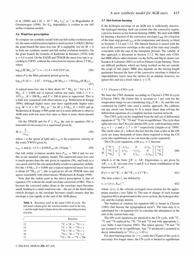
Table 4. Reactions used in the rapid CNO bi-cycle. Theleft-hand column gives the reaction number used in the text,i, and the right-hand column shows the corresponding nuclearreaction.

i Reaction

12 12C + 1H → 13N + γ

13 13C + 1H → 14N + γ

14 14N + 1H → 15O + γ

16 16O + 1H → 17F + γ

17 17O + 1H → 14N + 4He

3.7 Hot-bottom burning

If the hydrogen envelope of an AGB star is sufficiently massive,the hydrogen-burning shell can extend into the convective region,a process known as hot-bottom burning (HBB). We deal with HBBby burning a fraction of the convective envelope f HBB for a fractionof the time-step period f burn at the temperature and density as fittedin Sections 3.3.4 and 3.3.5. The burned fraction is mixed with therest of the convective envelope at the end of the time-step (usuallycoincident with the end of the interpulse period). The validity ofthis approach is discussed in Section 3.7.2. We burn only CNO,but HBB affects other elements via the NeNa and MgAl chains (seeKarakas & Lattanzio 2003) as well as lithium via pp-burning. Theseare difficult problems which are being worked on but are outsidethe scope of this paper. HBB also depends on the mixing-lengthparameter because the base of the convective envelope is linked tosuperadiabatic layers near the surface by an adiabat; however, weignore this and use a fixed value α = 1.75.

3.7.1 Clayton’s CNO cycle

We burn the CNO elements according to Clayton’s CNO bi-cycle(Clayton 1983). He claims this is accurate to 1 per cent for thetemperature range we are considering (log10T/K < 8), and this wasconfirmed by GdJ93 who used a similar approach. We calibrateout any errors (see Section 4). It is much faster than solving thedifferential equations of a complete nuclear reaction network.

The CNO cycle can be simplified from the full set of differentialequations if 13N, 15N, 15O and 17F are in equilibrium. The cycle thensplits into two, the CN cycle and the ON cycle, with branching ratiosαCN = 1 − γ and γ � 7 × 10−4 respectively (Angulo et al. 1999).The small value of γ reflects the fact that the time-scales in the ONcycle are many thousands of times those required to bring the CNcycle into equilibrium so we can treat the cycles separately.

The CN cycle equations, with αCN = 1, become

d

dt

[ 12C13C14N

]=

[−1/τ12 0 1/τ14

1/τ12 −1/τ13 00 1/τ13 −1/τ14

][ 12C13C14N

](60)

which is of the form ddt U = �U . Eigenvalues λi are given by

�U i = λi U i (no sum over i) and U is a linear combination of theeigenvectors U i, so

U (t) = Aeλ1tU 1 + Beλ2tU 2 + Ceλ3tU 3. (61)

The time-scales τ i are defined by

τi = (〈σv〉i XH1)−1 , (62)

where 〈σv〉i is the velocity-averaged cross-section for the appro-priate reaction i (see Table 4). The rate of change of each isotope(equation 60) is proportional to the cross-section, the hydrogen den-sity and the isotope density.

The method of solution for equation (60) is found in Clayton(1983) (but beware the typographical error!). The time-step δt issubstituted for t in equation (61) to calculate the abundances at theend of the current time-step.

The ON cycle equations are identical to the CN cycle, with 12C,13C and 14N replaced by 14N, 16O and 17O and with appropriate τ i

(see Table 4 and Clayton 1983). The minor species 15N and 17Oare assumed to be in equilibrium. Any 17F produced is assumed todecay immediately to 17O (τ 1/2 ≈ 65 s).

For short burning times (δt < τ 12) only the CN part of the cycle isnecessary. For longer times, the CN cycle is burned to equilibrium

C© 2004 RAS, MNRAS 350, 407–426

416 R. G. Izzard et al.

before the ON cycle is activated. Even in the most massive AGBstars undergoing vigorous HBB, XO16 does not change much sothe ON cycle never approaches equilibrium. Nuclear reaction ratesare taken from the formulae in the NACRE compilation (Anguloet al. 1999) except the beta decay constants which are taken fromthe compilation of Tuli (2000). The rates compare well to table 5.3(p. 393) of Clayton (1983).

3.7.2 Thin shell burning versus whole envelopeburning approximation

Between pulses the convective envelope of an AGB star turns overmany thousands of times. It is impossible to model this using littleCPU time because the burn → mix → burn → mix . . . process iscomputationally expensive, especially if the code is to be extendedto more isotopes than just 1H, 4He and CNO. Given the uncertaintiesinvolved in convective mixing and local mixing at the base of theenvelope, it is simpler and preferable to approximate the burning(many times) of a thin HBB layer at the base of the convectiveenvelope with a single burning of a larger portion of the envelope.

This can be justified by considering the size of the HBB region.For a 5-M� star d log10(T/K)/dm at the base of the envelope istypically 3 × 103M−1� . HBB ceases at log10(T/K) ≈ 7.6 and thetemperature at the base of the envelope is typically log10(T/K) ≈8 for most of the TPAGB. So �MHBB ≈ 10−4M�. This is muchsmaller than the size of the convective envelope (about 4 M� for a5-M� star), so the HBB shell can be considered as thin.

When the thin HBB shell is burned and then mixed into the enve-lope the abundances in the envelope are essentially unchanged. Onlyonce a significant number of mixings (of the order Menv/�MHBB)have occurred will the envelope abundances change noticeably, soin our approximation we burn a fraction of the envelope, f HBB, fora fraction of the interpulse period time f burn and fit f HBB and f burn toour full stellar evolution models. In reality, some parts of the enve-lope burn more than once but this is absorbed into the calibration off HBB. The burned shell and the rest of the envelope are mixed at theend of the time-step.

To calibrate the model we allow mixing 10 times per interpulseperiod so the shape of the abundances versus time profiles betweenpulses can be observed. The code is designed so that the result isidentical to that obtained if there is only one mixing per interpulse inthe way that the code is expected to be used in population synthesisruns.

Note that this technique differs from that of GdJ93 where theaverage abundance rather than the final abundance between time 0and f burnτ ip is mixed into the envelope.

4 H B B C A L I B R AT I O N A N D C O M PA R I S O NO F S Y N T H E T I C M O D E L S W I T H F U L LE VO L U T I O NA RY M O D E L S

The free parameters,

(i) f HBB – the fraction of the envelope of the star that is burned inthe HBB shell,

(ii) f burn – the fraction of the interpulse period for which the HBBshell burns,

(iii) f DUP – the fraction of the dredged-up material that ishydrogen-burned before being mixed into the envelope to simulatedredge-up of the hydrogen shell in low-Z stars,

(iv) f DUP,burn – the fraction of the interpulse period for which thedredged-up material is burned, and

Table 5. Burning time 106f burn as a fraction of the interpulse period fordifferent masses and metallicities. The first row of numbers for each Z arethe ranges narrowed down by the MC runs. The second row of numbers areused to fit a relation to M1TP and Z. f burn = 0 for M1TP < 3.5 M�.

Z ↓ M1TP/M� → 3.5 4.0 5.0 6.0 6.5

0.02 – – 0.1–0.5 0.5–0.6 0.4–1.00.3 0.55 0.7

0.008 0 <0.2 0.6–1.0 0.8–1.00 0.1 0.8 0.9

0.004 0 0.15–0.5 0.5–1.0 0.8–100 0.3 0.75 0.9

(v) N rise – the factor used to define how quickly the HBB tem-perature reaches T max,

are to be calibrated to our full stellar evolution models.Previous authors (e.g. GdJ93) have used constant values for f HBB,

f burn, f DUP and f DUP,burn, with a different prescription for the tem-perature (not requiring N rise). Here we assume that these valuesdiffer for each star, so we attempt to parameterize them in termsof M1TP and Z. Often we quote 106f burn instead of f burn becausef burn � 10−6.

4.1 Calibration method

A Monte Carlo (MC) method is used to test the above free parameterswith ranges 0.0 < f HBB < 1.0, 0.0 < 106f burn < 10.0 and 0 < N Trise <

20. f DUP and f DUP,burn are chosen to be zero and are only increasedwhen necessary.

A weighted sum of squares is constructed from our full stellarevolution model nucleosynthesis data versus the corresponding syn-thetic model nucleosynthesis results to enable comparison betweenMC model runs. A score = (

∑i wi si )−1 is defined such that higher

numbers mean a better fit where the weights are wi = (wC12, wC13,wN14, wO16, wC/O, wC12/C13) = (1, 10, 1, 1, 5, 5) and si is the sum ofsquares difference between our full stellar evolution and syntheticmodels for the isotope (or ratio) i. The ratios XC12/XC13 and XC/XO

are weighted preferentially because these are important observednucleosynthetic constraints on AGB stars. 13C is also boosted be-cause its abundance is small. 1D slices and 2D projections of theresulting parameter space are then examined and compared withthe best fit obtained by this method. Human intervention comes lastbut proves invaluable when trying to fit the details. Appendix B7

contains the details of the calibration results.

4.2 Free parameter Heaven or Hell

The results of the MC runs for each star are shown in Tables 5, 6and 7. Ranges are given when the MC technique cannot distinguisha unique solution. In such cases we choose a value that aids the fitof the free parameter to M1TP and Z or such that 106f burn ≈ f HBB.The chosen value is shown under the range. If the value is ‘–’ thenthere is no HBB so f DUP = f burn = 0.0. Where no value is giventhere is no full stellar evolution model with which to compare. It isnot possible to use the best MC values for every star because thereis too much non-systematic scatter.

7 http://www.blackwellpublishing.com/products/journals/suppmat/mnr/mnr7446/mnr7446sm.htm

C© 2004 RAS, MNRAS 350, 407–426

A new synthetic model for AGB stars 417

Table 6. Envelope mass fraction exposed to HBB, f HBB, for differentmasses and metallicities. The first row of numbers for each Z are the rangesnarrowed down by the MC runs. The second row of numbers are used to fita relation to M1TP and Z. f HBB = 0 for M1TP < 3.5 M�.

Z ↓ M1TP/M� → 3.5 4.0 5.0 6.0 6.5

0.02 – – 0.1–0.4 0.65 0.3–1.00.25 0.65 0.7

0.008 0 0.1–0.2 0.4–1.0 0.7–1.00 0.15 0.7 0.85

0.004 <0.1 0.1–0.5 0.8–1.0 0.75–1.00.1 0.3 0.9 0.85

Table 7. Temperature rise factor N rise for different masses and metallicities.The first row of numbers for each Z are the ranges narrowed down by theMC runs. The second row of numbers are used to fit a relation to M1TP andZ. N rise is undefined for M1TP < 3.5 M� (because f burn = f HBB = 0).

Z ↓ M1TP/M� → 3.5 4.0 5.0 6.0 6.5

0.02 – – ∼3 <1 1–23 0.5 1.5

0.008 �6 ∼6 ∼2.5 ∼26 6 2.5 2

0.004 ∼6 ∼3 <2 <16 3 2 1

The values for f HBB and f burn are zero for M1TP < 3.5 M� witha step up to about 0.9 at M1TP ≈ 4.5 M� and a slight metallicitydependence. These can be reasonably well fitted to a function f 63

similar to a Fermi function:

f63 = (a63 Z + b63)

1 + (c63 Z + d63)(e63 Z+g63−M1TP/M�). (63)

The f 63 parameter for f HBB or 106f burn is then given by max(f 63,0.0).

N rise is fitted to a quadratic in M1TP and z = min(Z, 0.02):

Nrise = max[a64(M1TP/M�)2 + b64(M1TP/M�)

+ c64z + d64z2 + e64, 0]. (64)

The maximum value for Z is necessary to maintain the behaviour ofthe function at higher metallicity. Equation (64) reaches a minimumvalue at around M1TP = 6 M� and is assumed to be valid for masseshigher than this.

For Z < 0.004 we include some immediate burning of dredge-upmaterial.

4.3 Sensitivity to f HBB, f burn and Nrise

With the model described above and an appropriate choice of f HBB,f burn and N rise, it is possible to match our full stellar evolution modelsto our synthetic models quite accurately. Problems occur with thefitted values of f HBB, f burn and N rise because minor deviations inthe fit of the free parameters produce very different output (thesensitivity does not help us to pin down unique values for f burn andf HBB because of their inherent degeneracy). For example, if N rise

is too small then 13C rises and falls too early in the M i = 6 M�stars. If f burn is even slightly too small then the ON cycle does

-2.8

-2.7

-2.6

-2.5

-2.4

-2.3

-2.2

-2.1

0 0.5 1 1.5 2 2.5 3

log 1

0(X

C12

)

Time / 105 yrs

Figure 6. 12C abundance versus time for M i = 5 M�, Z = 0.02 with varyingf HBB = f fit

HBB + �f , with −0.13 < �f < 0.13. The fitted value of f HBB isslightly wrong, but this only gives a maximum error of 0.15. The solid lineis the full stellar evolution model; the other three lines are �f = −0.13, 0and +0.13 denoted with pluses, crosses and open squares respectively.

not get switched on.8 If f burn is slightly too large then more 14Nis produced at the expense of 12C and 13C. A slight rise in f HBB

causes a large rise in HBB products, especially 14N. The sensitivityto f HBB and f burn is compounded when both are erroneous in the samedirection.

A change to f HBB affects the 12C surface abundance evolution forM i = 5 M�, Z = 0.02 (see Fig. 6). An increased f HBB better fitsthe drop in 12C which occurs when HBB sets in, but by the endof the evolution the surface abundances are not very different. Atmost XC12 is wrong by a factor of 1.4 at any point over the entireevolution, while overall it changes by a factor of 5. Final 13C and14N have a similar scatter in log10X of about 0.15. These effectsare hardly visible in the case of the M i = 6 M�, Z = 0.02 starand, because no burning occurs at all at M i/M� = 4, it is only inthe M i/M� ≈ 4.5–5 transition zone that we have to worry aboutthis.

Alteration of the burning time, f burn, has essentially the sameeffect as a similar change in f HBB with the exception of oxygenwhich is burned in the ON cycle when f burn is long enough. Theamount of 16O burned for M i = 6 M�, Z = 0.02 is very smallin our full stellar evolution models (� log10XO16 = −0.04). This isabout twice the size of the spread with �f burn = ±0.13 so we shouldnot read too much into this. Significant oxygen burning occurs forM i = 6 M�, Z = 0.004 but the standard model deals quite well withthis (see Fig. 7). The carbon and nitrogen abundances are weaklyaffected at M i = 6 M� but at the transition mass (M i = 5 M� forZ = 0.02, M i = 4 M� for Z = 0.004) the surface abundance issensitive to f burn.

In summary, stars in the zone of transition between non-HBB andHBB (M i = 4 M� for Z = 0.004, M i = 5 M� for Z = 0.02) arethe most troublesome when it comes to errors in the fit to f HBB andf burn. However, this transition is quite sharp, so not too many starsin a population would have the wrong surface abundances.

8 This is not a huge problem (except for M i > 6 M�) because most stars donot change their surface oxygen abundance significantly over their lifetime.For M i > 6 M� and low Z this could be a source of worry.

C© 2004 RAS, MNRAS 350, 407–426

418 R. G. Izzard et al.

-3.8-3.7-3.6-3.5-3.4-3.3-3.2-3.1

-3-2.9-2.8-2.7

0 0.5 1 1.5 2 2.5 3 3.5 4 4.5

log 1

0(X

O16

)

Time / 105 yrs

Figure 7. 16O abundance versus time for the M i = 6 M�, Z = 0.004models, with f burn set to f fit

burn +�f , where −0.13 <�f < 0.13. Our standardsynthetic model (�f = 0) does a reasonable job of reproducing the full stellarevolution model. The solid line is the full stellar evolution model; the othersfrom top to bottom are �f = −0.13, 0 and +0.13 denoted with pluses,crosses and open squares respectively.

4.3.1 Temperature sensitivity

If the fit to the temperature of the HBB layer (Section 3.3.4) isallowed to vary even by a tiny amount, while the other free parame-ters are kept constant, CNO element production varies significantly.

Figure 8. 12C, 13C, 14N and 16O surface abundances versus time for M i = 6 M�, Z = 0.02 with varying temperature factor 0.98 < fT < 1.02. The solid lineis our full stellar evolution model. The dashed lines represent fT = 0.98 to 1.02 in 0.01 increments, from top to bottom (pluses, crosses, open squares, filledsquares and open circles respectively). See text for details.

To show this, log10T max is allowed to vary from the fitted valueby a factor of 0.98 < fT < 1.02, just 2 per cent variations (5 percent in T max), and the abundance versus time profiles are comparedfor the case M i = 6 M�, Z = 0.02 which would ordinarily un-dergo large amounts of HBB (see Fig. 8). We do not always ex-pect fT = 1.00 to be the best fit because in reality the HBB layerhas a temperature profile while in our synthetic model it does not.Note that the log10T max limit of 7.95 has been disabled for thesetests, leading to numerical problems due to imaginary eigenvaluesat fT = 1.02.

(i) The final 12C is not greatly affected by temperature changesbut fT = 0.98 effectively switches off HBB. Paradoxically fT = 1.02burns less 12C than fT = 1.01 during most of the evolution. Thisis because fT = 1.02 puts the temperature above the log10(T/K) =7.95 limit of applicability of the burning code. The best fit is forfT = 1.0.

(ii) 13C is affected in a more subtle way. At low temperaturemore 13C is produced by incomplete CNO cycling. At the highertemperatures this 13C is converted to 14N. The final abundances forfT > 1.0 are all similar because CN equilibrium is achieved, whilefor fT < 1.00 there has not been enough conversion of 13C to 14N.Again fT = 1.00 is the best fit.

(iii) The log of the final surface abundance of nitrogen variesfrom −2.55 at fT = 0.98 (the same as the abundance at thestart of the TPAGB) to −1.85 at fT = 1.02. The best fitis fT = 1.01 although fT = 1.00 is not too bad. For fT �

C© 2004 RAS, MNRAS 350, 407–426

A new synthetic model for AGB stars 419

1.01 nitrogen abundances are high because of excessive ONcycling.

(iv) Out of all the CNO elements the surface oxygen abundancevaries the most with temperature. For fT � 1.00 there is little changein oxygen abundance, just as in our full stellar evolution models. Anincrease in the value of fT to just 1.02 causes the surface oxygenabundance to drop by a factor of 10. This is not seen in our full stellarevolution models, so a value of fT = 1.00 is certainly justified whilefT = 1.01 also gives too large a drop.

4.3.2 Dangerous interpolations and extrapolations

The TPAGB code is designed to be inserted into the rapid stellarevolution code, which deals with both single and binary stars for0.1 � M i/M� � 100.0 and 0.0001 � Z � 0.03. This means thatthe expressions in the TPAGB code, developed here for 1 � M i/M�� 6.5 and 0.004 � Z � 0.02, or M i � 2.25 M�, Z = 0.0001, mustbe interpolated over a factor of 40 in Z, or extrapolated beyondZ = 0.004 for M � 2.5 M�, into regimes where they have not beenfitted to full stellar evolution models. Our expressions are designedto give sensible results when extrapolated or interpolated to lowmetallicity, but we have no way to tell if the results are correct.

5 D R E D G E - U P C A L I B R AT I O N A N DC O M PA R I S O N W I T H O B S E RVAT I O N S

5.1 Carbon stars

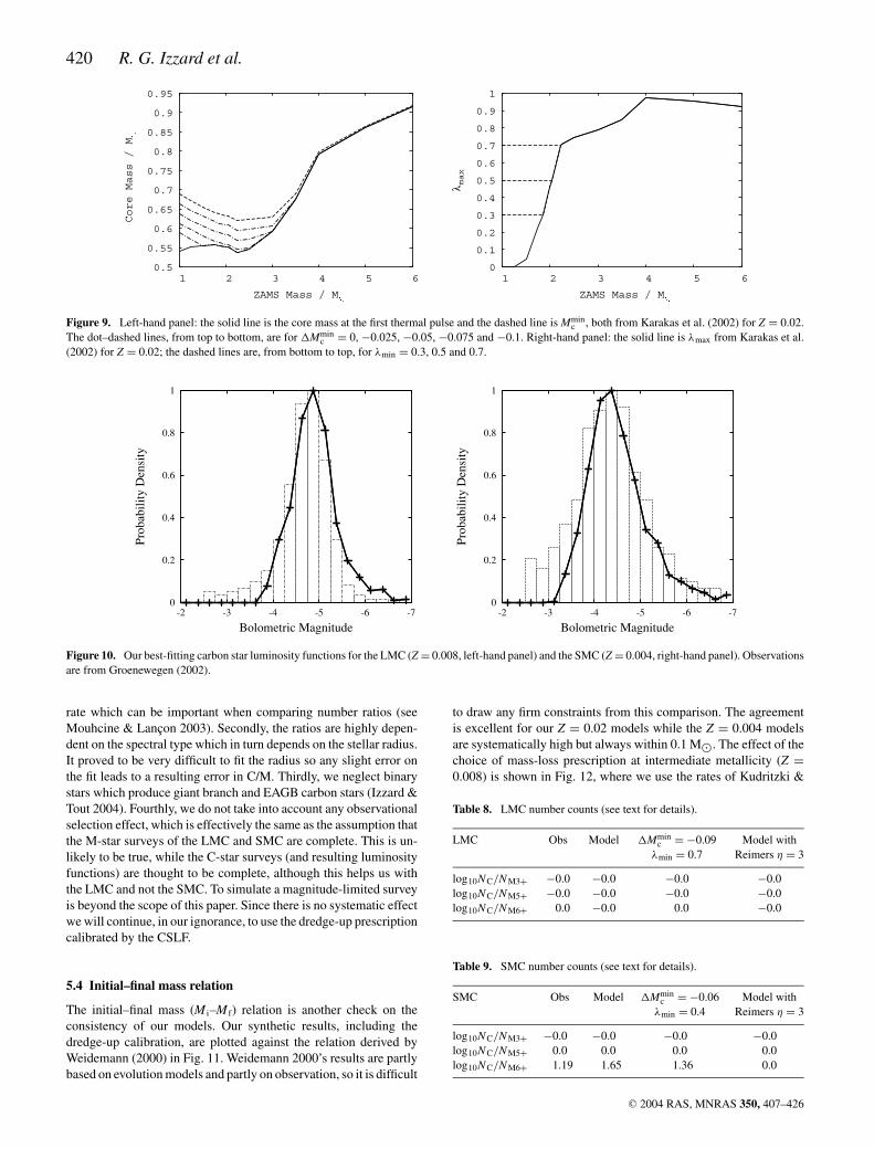
The carbon star luminosity function (CSLF) is defined as the numberof carbon stars per unit bolometric magnitude for a particular popu-lation, i.e. it is a probability density function. We model a populationof stars in the mass range 0.5 � M i/M� � 8.0 where the probabil-ity for each star is taken from the initial mass function of Kroupa,Tout & Gilmore (1993) (KTG93, see also Appendix A7) and we as-sume a constant star formation rate. Results are compared with theLarge Magellanic Cloud (LMC) (Z = 0.008) and Small MagellanicCloud (SMC) (Z = 0.004) data taken from Groenewegen (2002)(2002; see also Groenewegen 1999). The theoretical distributionsare binned identically to the observed data in 0.25-mag bins. Alldistributions are normalized such that the integrated probability is1.0 (so are independent of the star formation rate if we assume it isconstant). Because the bin widths are fixed, the probability densityis directly proportional to the probability per bin (i.e. the number ofstars per bin) so is directly compared to the (suitably normalized)observations.

It turns out that to fit the dim carbon stars with bolometric magni-tude less than −3 we have to introduce a correction to the luminosityto deal with post-flash minima. This is a factor of the form

fL = 1 − 0.5 × min

[1, exp

(−3

τ

τip

)], (65)

which is activated for the first 10 pulses to mimic the full evolutionmodels. After about 10 pulses the luminosity dip lasts for a shorttime and is not of large enough magnitude to contribute to the dimCSLF tail (the maximum dip seen in the full evolution models isa factor of 0.5L equivalent to 0.75 mag). Extending the dip to allpulses does not significantly change the model CSLF of either theSMC or the LMC. The dimmest of carbon stars with magnitudeabout −3 cannot be fitted at all because they are probably extrinsiccarbon stars in binary systems (Izzard & Tout 2004). Note that inorder to resolve the dips the time-step is reduced to at most one-tenthof the interpulse period.

5.2 Modification of dredge-up parameters

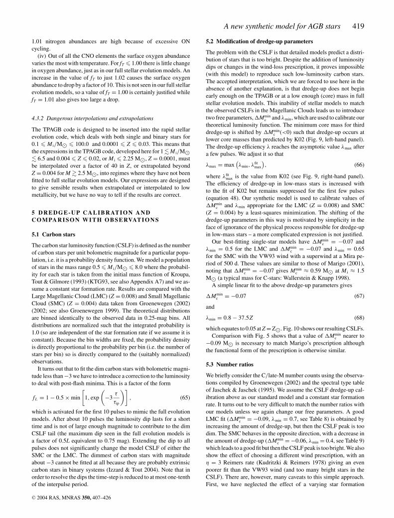
The problem with the CSLF is that detailed models predict a distri-bution of stars that is too bright. Despite the addition of luminositydips or changes in the wind-loss prescription, it proves impossible(with this model) to reproduce such low-luminosity carbon stars.The accepted interpretation, which we are forced to use here in theabsence of another explanation, is that dredge-up does not beginearly enough on the TPAGB or at a low enough (core) mass in fullstellar evolution models. This inability of stellar models to matchthe observed CSLFs in the Magellanic Clouds leads us to introducetwo free parameters, �Mmin

c and λmin, which are used to calibrate ourtheoretical luminosity function. The minimum core mass for thirddredge-up is shifted by �Mmin

c (<0) such that dredge-up occurs atlower core masses than predicted by K02 (Fig. 9, left-hand panel).The dredge-up efficiency λ reaches the asymptotic value λmax aftera few pulses. We adjust it so that

λmax = max(λmin, λ

fitmax

), (66)

where λfitmax is the value from K02 (see Fig. 9, right-hand panel).

The efficiency of dredge-up in low-mass stars is increased withto the fit of K02 but remains suppressed for the first few pulses(equation 48). Our synthetic model is used to calibrate values of�Mmin

c and λmin appropriate for the LMC (Z = 0.008) and SMC(Z = 0.004) by a least-squares minimization. The shifting of thedredge-up parameters in this way is motivated by simplicity in theface of ignorance of the physical process responsible for dredge-upin low-mass stars – a more complicated expression is not justified.

Our best-fitting single-star models have �Mminc = −0.07 and

λmin = 0.5 for the LMC and �Mminc = −0.07 and λmin = 0.65

for the SMC with the VW93 wind with a superwind at a Mira pe-riod of 500 d. These values are similar to those of Marigo (2001),noting that �Mmin

c = −0.07 gives Mminc ≈ 0.59 M� at M i ≈ 1.5

M� (a typical mass for C-stars: Wallerstein & Knapp 1998).A simple linear fit to the above dredge-up parameters gives

�Mminc = −0.07 (67)

and

λmin = 0.8 − 37.5Z (68)

which equates to 0.05 at Z = Z�. Fig. 10 shows our resulting CSLFs.Comparison with Fig. 5 shows that a value of �Mmin

c nearer to−0.09 M� is necessary to match Marigo’s prescription althoughthe functional form of the prescription is otherwise similar.

5.3 Number ratios

We briefly consider the C/late-M number counts using the observa-tions compiled by Groenewegen (2002) and the spectral type tableof Jaschek & Jaschek (1995). We assume the CSLF dredge-up cal-ibration above as our standard model and a constant star formationrate. It turns out to be very difficult to match the number ratios withour models unless we again change our free parameters. A goodLMC fit (�Mmin

c = −0.09, λmin = 0.7, see Table 8) is obtained byincreasing the amount of dredge-up, but then the CSLF peak is toodim. The SMC behaves in the opposite direction, with a decrease inthe amount of dredge-up (�Mmin

c = −0.06, λmin = 0.4, see Table 9)which leads to a good fit but then the CSLF peak is too bright. We alsoshow the effect of choosing a different wind prescription, with anη = 3 Reimers rate (Kudritzki & Reimers 1978) giving an evenpoorer fit than the VW93 wind (and too many bright stars in theCSLF). There are, however, many caveats to this simple approach.First, we have neglected the effect of a varying star formation

C© 2004 RAS, MNRAS 350, 407–426

420 R. G. Izzard et al.

0.5

0.55

0.6

0.65

0.7

0.75

0.8

0.85

0.9

0.95

1 2 3 4 5 6

Core Mass / M

ZAMS Mass / M

0

0.1

0.2

0.3

0.4

0.5

0.6

0.7

0.8

0.9

1

1 2 3 4 5 6

λ max

ZAMS Mass / M

Figure 9. Left-hand panel: the solid line is the core mass at the first thermal pulse and the dashed line is Mminc , both from Karakas et al. (2002) for Z = 0.02.

The dot–dashed lines, from top to bottom, are for �Mminc = 0, −0.025, −0.05, −0.075 and −0.1. Right-hand panel: the solid line is λmax from Karakas et al.

(2002) for Z = 0.02; the dashed lines are, from bottom to top, for λmin = 0.3, 0.5 and 0.7.

0

0.2

0.4

0.6

0.8

1

-7-6-5-4-3-2

Prob

abili

ty D

ensi

ty

Bolometric Magnitude

0

0.2

0.4

0.6

0.8

1

-7-6-5-4-3-2

Prob

abili

ty D

ensi

ty

Bolometric Magnitude

Figure 10. Our best-fitting carbon star luminosity functions for the LMC (Z = 0.008, left-hand panel) and the SMC (Z = 0.004, right-hand panel). Observationsare from Groenewegen (2002).

rate which can be important when comparing number ratios (seeMouhcine & Lancon 2003). Secondly, the ratios are highly depen-dent on the spectral type which in turn depends on the stellar radius.It proved to be very difficult to fit the radius so any slight error onthe fit leads to a resulting error in C/M. Thirdly, we neglect binarystars which produce giant branch and EAGB carbon stars (Izzard &Tout 2004). Fourthly, we do not take into account any observationalselection effect, which is effectively the same as the assumption thatthe M-star surveys of the LMC and SMC are complete. This is un-likely to be true, while the C-star surveys (and resulting luminosityfunctions) are thought to be complete, although this helps us withthe LMC and not the SMC. To simulate a magnitude-limited surveyis beyond the scope of this paper. Since there is no systematic effectwe will continue, in our ignorance, to use the dredge-up prescriptioncalibrated by the CSLF.

5.4 Initial–final mass relation

The initial–final mass (M i–M f) relation is another check on theconsistency of our models. Our synthetic results, including thedredge-up calibration, are plotted against the relation derived byWeidemann (2000) in Fig. 11. Weidemann 2000’s results are partlybased on evolution models and partly on observation, so it is difficult

to draw any firm constraints from this comparison. The agreementis excellent for our Z = 0.02 models while the Z = 0.004 modelsare systematically high but always within 0.1 M�. The effect of thechoice of mass-loss prescription at intermediate metallicity (Z =0.008) is shown in Fig. 12, where we use the rates of Kudritzki &

Table 8. LMC number counts (see text for details).

LMC Obs Model �Mminc = −0.09 Model with

λmin = 0.7 Reimers η = 3

log10N C/N M3+ −0.0 −0.0 −0.0 −0.0log10N C/N M5+ −0.0 −0.0 −0.0 −0.0log10N C/N M6+ 0.0 −0.0 0.0 −0.0

Table 9. SMC number counts (see text for details).

SMC Obs Model �Mminc = −0.06 Model with

λmin = 0.4 Reimers η = 3

log10N C/N M3+ −0.0 −0.0 −0.0 −0.0log10N C/N M5+ 0.0 0.0 0.0 0.0log10N C/N M6+ 1.19 1.65 1.36 0.0

C© 2004 RAS, MNRAS 350, 407–426

A new synthetic model for AGB stars 421

0.5

0.6

0.7

0.8

0.9

1

1.1

1 2 3 4 5 6 7 8

Mf /

M

Mi / M

Z=0.02Z=0.008Z=0.004

Figure 11. Final mass versus initial mass for stars with 0.5 � M i/M�� 8 with metallicities 0.02 (squares), 0.008 (circles) and 0.004 (triangles)as calculated with the synthetic model (including dredge-up calibration).The solid line shows data from Weidemann (2000). Above M i ≈ 7 M� thefinal mass is strongly metallicity-dependent because low-metallicity starsexplode as supernovae on the EAGB, forming more massive neutron starsrather than white dwarfs.

0.5

0.6

0.7

0.8

0.9

1

1.1

1 2 3 4 5 6 7 8

Mf /

M

Mi / M

Reimers η=1Reimers η=5

Blöcker

Figure 12. Final mass versus initial mass for Z = 0.008 with varyingTPAGB mass-loss prescriptions: squares and circles are Reimers’ rates withη = 1 and 5 respectively; triangles are Blocker’s rate with η = 0.1.

Reimers (1978) and Blocker (1995). No single mass-loss relationgives the best agreement, but a Reimers η = 1 rate is discrepant bymore than 0.1 M� for M i � 3 M�, perhaps ruling this out.

5.5 White dwarf mass distribution

The observed white dwarf mass distribution provides an additionalconstraint on our models. The inherent uncertainty in the initial–finalmass relation, which is due to the use of evolutionary models to cal-culate an initial mass, is removed. The comparison of our syntheticwhite dwarf mass distribution with observations is shown in Fig. 13.The observations are compiled from Bergeron, Saffer & Liebert(1992), Bergeron, Liebert & Fulbright (1995), Bragaglia, Renzini& Bergeron (1995), Dreizler & Werner (1996), Bergeron, Ruiz &

0

0.1

0.2

0.3

0.4

0.5

0.6

0.7

0.8

0.9

1

0.5 0.6 0.7 0.8 0.9 1 1.1 1.2

WD Mass

Z=0.02Z=0.008Z=0.004

Figure 13. The white dwarf mass distribution. The boxed histogram showsthe observations; the lines show our synthetic results for Z = 0.02 (squares),0.008 (circles) and 0.004 (triangles).

Leggett (1997), Finley, Koester & Basri (1997), Marsh et al. (1997),Vennes et al. (1997), Napiwotzki, Green & Saffer (1999), Vennes(1999), Bergeron, Leggett & Ruiz (2001), Claver et al. (2001) andSilvestri et al. (2001), with no attempt to take into account any ob-servational selection effects such as dimming of old white dwarfs orsystematic biases such as the effect of a binary companion, metal-licity or errors inherent in different white dwarf mass determinationtechniques (although for duplicate stars the newer data are believedover the old). The data are plotted as a histogram in 10 bins, with anequal number of stars in each bin. Our synthetic model curves forZ = 0.02, 0.008 and 0.004 are calculated with 105stars for eachmetallicity between 0.1 and 8.0 M� and are binned in an identicalway. Our dredge-up calibration of Section 5.1 is used. The initialmass function of KTG93 is used to calculate the contribution ofeach star to the histogram, and no attempt is made to mimic selec-tion effects. The peak of the observations and theoretical curves arenormalized to 1.0.

The peak position of the mass distribution is matched well by oursynthetic models. We have a dearth of white dwarfs above 0.7 M�and below about 0.55 M�. These are probably due to the omissionof binary stars from our analysis. Binary-induced mass loss leads tolow-mass helium white dwarfs and mergers to high mass (possiblyoxygen–neon) white dwarfs.

6 S I N G L E S TA R Y I E L D S

In this section we calculate stellar yields appropriate for use in galac-tic chemical evolution models. We compare these yields with ourfull stellar evolution model yields and previously published yieldsof van den Hoek & Groenewegen (1997) and Marigo (2001).

6.1 Calculation of yields

The yield of isotope j from a star can be represented simply as themass expelled into the interstellar medium in time t:

�M j =∫ t

0

M j dt, (69)

or as a function of the initial mass and abundance:

p( j, Mi) = 1

Mi

∫ t

0

M�X j dt, (70)

C© 2004 RAS, MNRAS 350, 407–426

422 R. G. Izzard et al.

-0.0025

-0.002

-0.0015

-0.001

-0.0005

0

Yie

ld

Z=0.02

1H

Z=0.008 Z=0.004

0

0.0005

0.001

0.0015

0.002

Yie

ld

4He

-0.0002

0

0.0002

0.0004

0.0006

0.0008

Yie

ld

12C

0

5e-06

1e-05

1.5e-05

Yie

ld

13C

0

5e-05

0.0001

0.00015

0.0002

1 2 3 4 5 6 7 8

Yie

ld

M / M

14N

1 2 3 4 5 6 7 8

M / M

1 2 3 4 5 6 7 8

M / M

Figure 14. Synthetic HBB-calibrated, non-dredge-up-calibrated, initial mass function-weighted model yields yj (solid lines) and our full stellar evolutionmodel yields (dashed lines with crosses) versus initial mass for 1H, 4He, 12C, 13C and 14N and Z = 0.02, 0.008 and 0.004.

where M i is the initial mass of the star and �Xj = Xj(t) − Xj(0) isthe change in surface abundance of species j between its birth andtime t. The latter aids comparison with the models of van den Hoek& Groenewegen (1997) and Marigo (2001). Note that both theseyields are independent of the initial mass function. A more usefuldefinition of the yield is

y j = dY j

dM= ξ (Mi)

∫ t

0

M�X j dt = ξ (Mi)Mi p( j, Mi), (71)

where ξ (M i) is the initial mass function [e.g. KTG93; ξ (M i) hasunits M−1� so yj is dimensionless].

The integral

Y j =∫ M2

M1

y j dM (72)

is the total enrichment (in M�) of species j by a population of starsbetween masses M1 and M2.

The yield in equations (70) and (71) can be negative if an isotopeis consumed (e.g. the hydrogen yield is always negative).

C© 2004 RAS, MNRAS 350, 407–426

A new synthetic model for AGB stars 423

-1e-07

-8e-08

-6e-08

-4e-08

-2e-08

0

Yie

ld

15N

-1.5e-05

-1e-05

-5e-06

0

5e-06

1e-05

Yie

ld

16O

-1e-070

1e-072e-073e-074e-075e-076e-077e-078e-07

Yie

ld

17O

0

2e-05

4e-05

6e-05

8e-05

0.0001

1 2 3 4 5 6 7 8

Yie

ld

M / M

22Ne

1 2 3 4 5 6 7 8

M / M

1 2 3 4 5 6 7 8

M / M

Figure 15. As Fig. 14, but for 15N, 16O, 17O and 22Ne.

The contributions to the yields are calculated from equation (71)at each time-step. The initial mass is in the range 0.1 � M i/M�� 8.0. The stars are evolved for 16 Gyr and the yields (withoutsupernova yields) shown are for the entire stellar lifetime. Full tablesof yields are in Appendix D.9 We show the yields from our full stellarevolution models without attempting to compensate for mass lossthat would occur after model breakdown (see Karakas & Lattanzio2003).

6.2 Results

Most of the mass from each star that is expelled in the stellar windis hydrogen or helium, and most of this is expelled in the TPAGBstage of the evolution of the star. Stars with M i � 7–8 M� do nothave a TPAGB stage, but explode as supernovae first, so the stellarwind yield from these stars is negligible. Stars with M i � 0.8 M�do not evolve to the TPAGB in 16 Gyr so also have negligible

9 http://www.blackwellpublishing.com/products/journals/suppmat/mnr/mnr7446/mnr7446sm.htm

yield. Comparison with the yields from (van den Hoek & Groe-newegen 1997, (HG97), Marigo (2001) M01) and our full stellarevolution models is made. The yields of HG97 were calculated us-ing a Kudritzki & Reimers (1978) mass-loss relation, with η = 4 (andη = 2 for Z = 0.004). The yields from M01 were calculated usingthe wind of VW93 (presumably with the M i > 2.5 M� correction)for Z = 0.019 (but we compare them with our Z = 0.02 models)and mixing length parameter αMLT = 1.68 rather than 1.75.

6.2.1 Comparison with our full stellar evolution models

Figs 14 and 15 compare our synthetic model yields (equation 71)with our full stellar evolution model yields using the HBB calibra-tion of Section 4, without the dredge-up calibration of Section 5.1and with the KTG93 initial mass function weighting. Our syntheticmodel does an excellent job of reproducing our full stellar evolutionmodels for all isotopes considered except 22Ne. Slight overproduc-tion of 12C, 13C and 14N for M i � 5 M� is due to small differencesbetween our synthetic and full evolution models. The spike in pro-duction of 13C at around M i ≈ 4–5 M� is not an anomaly – rather it

C© 2004 RAS, MNRAS 350, 407–426

424 R. G. Izzard et al.

-0.007-0.006-0.005-0.004-0.003-0.002-0.001

0

Yie

ld

Z=0.02

1H

Z=0.008 Z=0.004

0

0.001

0.002

0.003

0.004

0.005

Yie

ld

4He

0

0.0005

0.001

0.0015

0.002

Yie

ld

12C

05e-061e-05

1.5e-052e-05

2.5e-053e-05

3.5e-05

Yie

ld

13C

0

5e-05

0.0001

0.00015

0.0002

1 2 3 4 5 6 7 8

Yie

ld

M / M

14N

1 2 3 4 5 6 7 8

M / M

1 2 3 4 5 6 7 8

M / M

Figure 16. Our synthetic HBB- and dredge-up-calibrated model yields yj (solid lines) versus other models (circles from M01, squares from HG97, filledsymbols for η = 2, open symbols for η = 4) for 1H, 4He, 12C, 13C and 14N and Z = 0.02, 0.008 and 0.004. An initial mass function weighting is included.

is not resolved on our full stellar evolution model mass grid unlessit happens to lie on an integer multiple of M� (as is the case for Z =0.02). We do not include 22Ne destruction reactions so our syntheticyields are overestimates for M i � 4 M�.

6.2.2 Comparison with other models

We use the HBB and dredge-up calibrations made above (Sections 4and 5.1) to compare our synthetic model yields with those of M01and HG97. The yields are weighted with the KTG93 initial massfunction – see Figs 16 and 17 and Appendix A7.

For most isotopes our yields lie between the values given byM01 and HG97. Our synthetic models experience less dredge-upthan M01’s in the range 1 � M i/M� � 3, leading to a relativeunderproduction of carbon and oxygen, though slightly more thanHG97. The 13C spike position differs between our synthetic modelsand M01’s by 0.5 M� at Z = 0.004, suggesting that we invokeHBB at a slightly higher mass, and also by a factor of about 2.5(perhaps due to excess 12C seed). At lower metallicities (Z � 0.008)we overproduce nitrogen compared with the other yield sets, butM01 does not have AGB stars above 5 M� and our results arenot dissimilar to HG97’s Z = 0.004, η = 2 case (they publish no

C© 2004 RAS, MNRAS 350, 407–426

A new synthetic model for AGB stars 425

-1e-07

-8e-08

-6e-08

-4e-08

-2e-08

0

Yie

ld

15N

-2e-050

2e-054e-056e-058e-05

0.00010.000120.000140.00016

Yie

ld

16O

-1e-06-5e-07

05e-071e-06

1.5e-062e-06

2.5e-063e-06

Yie

ld

17O

0

5e-05

0.0001

0.00015

0.0002

0.00025

0.0003

1 2 3 4 5 6 7 8

Yie

ld

M / M

22Ne

1 2 3 4 5 6 7 8

M / M

1 2 3 4 5 6 7 8

M / M

Figure 17. As Fig. 16 but for 15N, 16O, 17O and 22Ne.

η = 2 yields for Z = 0.008). Our 15N agrees well with M01. The huge16O production at low mass in HG97’s data set for Z = 0.02 cannotbe reproduced, although otherwise our yields agree well except forthe lack of oxygen from dredge-up compared with M01 (also ourintershell abundance is on average about 1 per cent compared withMarigo’s 2 per cent). We produce negligible 17O compared with M01although the amount is still rather small. The initial mass function-weighted 22Ne yields show that the region of HBB (M i � 4–5 M�)is a relatively unimportant contributor to the total yield. It is alsopossible that the lower initial core masses from the Padova modelshave an effect on the evolution of M01’s models, with lower coremass leading to lower luminosity and so a longer TPAGB phasewith more dredge-up and enhanced CO yields.

7 C O N C L U S I O N S

We have presented a fast yet accurate synthetic model for TPAGBevolution based on state-of-the-art full evolution models. Yields cal-culated by the synthetic model and the full evolution model agreeclosely, with continuation of the synthetic model beyond the break-

down point of the detailed model for high-mass AGB stars. Cal-ibration of third dredge-up to the Magellanic Cloud carbon starluminosity functions forces us to reduce our theoretically derivedminimum mass for core mass by −0.07 M� and enforce a valueof at least 0.8 − 37.5Z on the maximum dredge-up efficiency λmax.The calibrated yields in general lie between the previously publishedyields of van den Hoek & Groenewegen (1997) and Marigo (2001),although our models produce more nitrogen and less carbon at lowmetallicity. Our synthetic model fits the initial–final mass relation towithin 0.1 M� and reasonably fits the observed white dwarf massdistribution (we require binary stars to fit it properly). The next stepis to include this synthetic model in the Hurley et al. (2002) binarycode, and much progress has already been made in this direction(Izzard & Tout 2004,2003).

AC K N OW L E D G M E N T S

We thank John Lattanzio, Maria Lugaro, Richard Stancliffe,Carolina Odman and especially the anonymous referee for usefuldiscussion, encouragement and suggestions. RGI thanks PPARC for

C© 2004 RAS, MNRAS 350, 407–426

426 R. G. Izzard et al.

a scholarship, Monash Mathematics Department for putting up withhim, and his own pocket for decent computing facilities. CAT thanksChurchill College for a fellowship.

R E F E R E N C E S

Anders E., Grevesse N., 1989, Geochim. Cosmochim. Acta, 53, 197Angulo C. et al., 1999, Nucl. Phys. A, 656, 3Bergeron P., Saffer R. A., Liebert J., 1992, ApJ, 394, 228Bergeron P., Liebert J., Fulbright M. S., 1995, ApJ, 444, 810Bergeron P., Ruiz M. T., Leggett S. K., 1997, ApJS, 108, 339Bergeron P., Leggett S. K., Ruiz M. T., 2001, ApJS, 133, 413Blocker T., 1995, A&A, 297, 727Blocker T., Schonberner D., 1991, A&A, 244, L43Boothroyd A. I., Sackmann I.-J., 1988, ApJ, 328, 632Bragaglia A., Renzini A., Bergeron P., 1995, ApJ, 443, 735Busso M., Gallino R., Lambert D. L., Travaglio C., Smith V. V., 2001, ApJ,

557, 802Chieffi A., Domınguez I., Limongi M., Straniero O., 2001, ApJ, 554, 1159Claver C. F., Liebert J., Bergeron P., Koester D., 2001, ApJ, 563, 987Clayton D. D., 1983, Principles of Stellar Evolution and Nucleosynthesis.

Univ. Chicago Press, ChicagoDray L. M., Tout C. A., Karakas A. I., Lattanzio J. C., 2003, MNRAS, 338,

973Dreizler S., Werner K., 1996, A&A, 314, 217Finley D. S., Koester D., Basri G., 1997, ApJ, 488, 375Forestini M., Charbonnel C., 1997, A&AS, 123, 241Frost C. A., 1997, PhD thesis, Monash UniversityFrost C. A., Lattanzio J. C., Wood P. R., 1998, ApJ, 500, 355Girardi L., Bressan A., Bertelli G., Chiosi C., 2000, A&AS, 141, 371 (G00)Groenewegen M. A. T., 1999, in Le Bertre T., Lebre A., Waelkens C., eds,

Proc. IAU Symp. 191, Asymptotic Giant Branch Stars. Astron. Soc. Pac.,San Francisco, p. 535

Groenewegen M. A. T., 2002, preprint (astro-ph/0208449)Groenewegen M. A. T., de Jong T., 1993, A&A, 267, 410 (GdJ93)Henry R. B. C., 2004, in McWilliam A., Rauch M., eds, Origin and Evolution

of the Elements. Cambridge Univ. PressHerwig F., 2000, A&A, 360, 952Hurley J., 2000, PhD thesis, Univ. CambridgeHurley J. R., Pols O. R., Tout C. A., 2000, MNRAS, 315, 543Hurley J. R., Tout C. A., Pols O. R., 2002, MNRAS, 329, 897 (H02)Iben I., Renzini A., 1983, ARA&A, 21, 271Iben I., Truran J. W., 1978, ApJ, 220, 980Iglesias C. A., Rogers F. J., 1996, ApJ, 464, 943Izzard R. G., Tout C. A., 2003, Publ. Astron. Soc. Aust., 20, 345Izzard R. G., Tout C. A., 2004, MNRAS, in press

Jaschek C., Jaschek M., 1995, The Behavior of Chemical Elements in Stars.Cambridge Univ. Press

Karakas A. I., Lattanzio J. C., 2003, Publ. Astron. Soc. Aust., 20, 279Karakas A. I., Lattanzio J. C., Pols O. R., 2002, Publ. Astron. Soc. Aust.,

19, 515 (K02)Kroupa P., Tout C., Gilmore G., 1993, MNRAS, 262, 545 (KTG93)Kudritzki R., Reimers D., 1978, A&A, 70, 227Lattanzio J. C., 1989, ApJ, 344, L25Lattanzio J. C., Frost C. A., Cannon R. C., Wood P. R., 1997, in Advances

in Stellar Evolution. Cambridge Univ. Press, p. 130Marigo P., 1999, in Le Bertre T., Lebre A., Waelkens C., eds, Proc. IAU Symp.

191, Asymptotic Giant Branch Stars. Astron. Soc. Pac., San Francisco,p. 53 (M99)

Marigo P., 2001, A&A, 370, 194 (M01)Marigo P., Bressan A., Chiosi C., 1998, A&A, 331, 564Marigo P., Girardi L., Bressan A., 1999a, A&A, 344, 123Marigo P., Girardi L., Weiss A., Groenewegen M. A. T., 1999b, A&A, 351,

161Marsh M. C. et al., 1997, MNRAS, 286, 369Mouhcine M., Lancon A., 2003,, MNRAS, 338, 572Mowlavi N., 1999, A&A, 350, 73Mowlavi N., Meynet G., 2000, A&A, 361, 959Mowlavi N., Jorissen A., Arnould M., 1998, A&A, 334, 153Napiwotzki R., Green P. J., Saffer R. A., 1999, ApJ, 517, 399Paczynski B., 1970, Acta Astron., 20, 47Press W. H., Teukolsky S. A., Vetterling W. T., Flannery B. P., 1992, Numer-

ical Recipes in C. The Art of Scientific Computing, 2nd edn. CambridgeUniv. Press, Cambridge

Renzini A., Voli M., 1981, A&A, 94, 175Russell S. C., Dopita M. A., 1992, ApJ, 384, 508Silvestri N. M., Oswalt T. D., Wood M. A., Smith J. A., Reid I. N., Sion E.

M., 2001, AJ, 121, 503Straniero O., Chieffi A., Limongi M., Busso M., Gallino R., Arlandini C.,

1997, ApJ, 478, 332Tuli J., 2000, Nuclear Wallet Cards. Brookhaven National Laboratoryvan den Hoek L. B., Groenewegen M. A. T., 1997, A&AS, 123, 305 (HG97)Vassiliadis E., Wood P. R., 1993, ApJ, 413, 641 (VW93)Vennes S., 1999, ApJ, 525, 995Vennes S., Thejll P. A., Galvan R. G., Dupuis J., 1997, ApJ, 480, 714Wagenhuber J., Groenewegen M. A. T., 1998, A&A, 340, 183Wallerstein G., Knapp G. R., 1998, ARA&A, 36, 369Weidemann V., 2000, A&A, 363, 647Wood P. R., Zarro D. M., 1981, ApJ, 247, 247

This paper has been typeset from a TEX/LATEX file prepared by the author.

C© 2004 RAS, MNRAS 350, 407–426